Macroprudential analysis of the financial system: the · PDF fileMacroprudential analysis of...

Macroprudential analysis of the financial system: the case of South Africa

Francis Selialia,1 Thabo Mbeleki2 and Kgomotso Matlapeng3

1. Introduction

Financial stability is crucial for sustained economic growth. Economic growth cannot be achieved without strong financial systems. Even with sound macroeconomic fundamentals, weak financial systems can destabilise economies, making them more vulnerable to external shocks. The interaction of financial markets and the real economy needs close monitoring since the instability of the financial system can be very costly. A smoothly operating, stable and efficient financial system is a major pillar for growth, output and employment.

Central banks have adopted macroprudential analysis as a widely used method of detecting vulnerabilities in the financial system. This involves, among other things, the identification of financial soundness indicators (FSIs) and the methods used to analyse them. Observing potential signs of heightened risks in the financial system is important for central banks, as they rely on such insights to be able to take both preventive measures and appropriate action in crisis management.

The rest of the paper is organised as follows. Section 2 defines macroprudential analysis and the FSIs. Section 3 provides methods of identifying FSIs. The main analytical tools are described in section 4. Section 5 discusses the methodology for modelling credit risk. Section 6 presents the bivariate regression results and a brief discussion of scenarios. Section 7 discusses the risk-bearing capacity of the banking sector and the model’s forecasting accuracy. The last section concludes.

2. Macroprudential analysis

Macroprudential analysis is a method of economic analysis that evaluates the health, soundness and vulnerabilities of a financial system. The analysis involves the assessment and monitoring of the strengths and vulnerabilities of financial systems using quantitative information, largely in terms of FSIs, and other economic indicators that provide a broader picture of economic and financial circumstances. The assessment takes into account both

1 South African Reserve Bank, Financial Stability Department, 370 Church Street, Pretoria, 0002, South Africa.

E-mail: [email protected]. Francis Selialia is an assistant general manager and head of the Macroprudential Analysis Division of the Financial Stability Department at the South African Reserve Bank. He joined the Bank in 1998 as an assistant economist in the Money and Banking Division of the Research Department. Later he joined the Monetary Policy Research Unit and was promoted to deputy economist. Before starting work at the South African Reserve Bank, he was a senior economist at the Central Bank of Lesotho and a deputy director at the South African National Treasury. He holds the following degrees: Master of Arts in economics and a postgraduate diploma in economic sciences from University College, Dublin, Ireland and a Bachelor of Arts in economics from the National University of Lesotho.

2 South African Reserve Bank, Financial Stability Department, 370 Church Street, Pretoria, 0002, South Africa. E-mail: [email protected].

3 South African Reserve Bank, Financial Stability Department, 370 Church Street, Pretoria, 0002, South Africa. E-mail: [email protected].

110 IFC Bulletin No 33

the risks facing the financial system and the system’s capacity to withstand shocks. It also involves establishing or investigating the linkages between the financial system and the real sector of the economy. Scenario analysis and stress tests are major components of this analysis and they help in determining the system’s sensitivity to economic shocks and its resilience to such shocks.

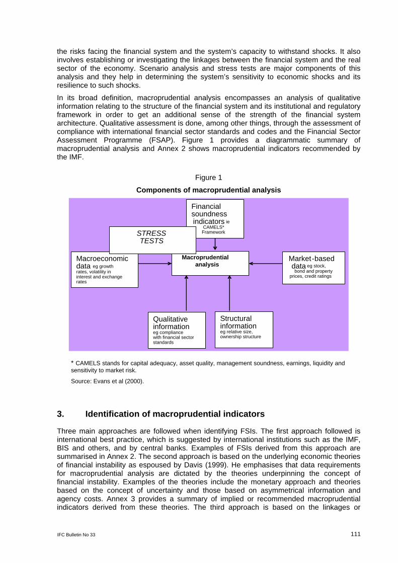
In its broad definition, macroprudential analysis encompasses an analysis of qualitative information relating to the structure of the financial system and its institutional and regulatory framework in order to get an additional sense of the strength of the financial system architecture. Qualitative assessment is done, among other things, through the assessment of compliance with international financial sector standards and codes and the Financial Sector Assessment Programme (FSAP). Figure 1 provides a diagrammatic summary of macroprudential analysis and Annex 2 shows macroprudential indicators recommended by the IMF.

Figure 1

Components of macroprudential analysis

Macroeconomic data eg growth rates, volatility in interest and exchange

Financial soundness indicators ie

CAMELS* Framework

Macroprudential analysis

Qualitative informationeg compliancewith financial sectorstandards

STRESSTESTS

Structural information eg relative size, ownership structure

Market - baseddata eg stock,

bond and property prices, credit ratings

rates

* CAMELS stands for capital adequacy, asset quality, management soundness, earnings, liquidity and sensitivity to market risk.

Source: Evans et al (2000).

3. Identification of macroprudential indicators

Three main approaches are followed when identifying FSIs. The first approach followed is international best practice, which is suggested by international institutions such as the IMF, BIS and others, and by central banks. Examples of FSIs derived from this approach are summarised in Annex 2. The second approach is based on the underlying economic theories of financial instability as espoused by Davis (1999). He emphasises that data requirements for macroprudential analysis are dictated by the theories underpinning the concept of financial instability. Examples of the theories include the monetary approach and theories based on the concept of uncertainty and those based on asymmetrical information and agency costs. Annex 3 provides a summary of implied or recommended macroprudential indicators derived from these theories. The third approach is based on the linkages or

IFC Bulletin No 33 111

interaction between the financial sector and other sectors of the economy. It is summarised with the aid of the circular flow of income and expenditure4 (Annex 4).

In all the approaches discussed above, the indicators should be analytically and empirically relevant, that is, there should be a sensible basis for expecting a relationship between the indicator and financial instability, and indicators should have predictive power or be classified as leading indicators in the sense that changes in one variable precede changes in another.

4. Assessment methods

Central banks in different countries use different techniques to assess and monitor the exposure of financial systems to different types of risks and shocks. As mentioned earlier, in most cases, stress tests and scenario analysis are the main methods used to determine the system’s sensitivity to economic shocks. Stress testing is a generic term describing various techniques used by financial firms to gauge potential vulnerability to exceptional but possible events.4 These methods are preferred because they perform a quantitative analysis of financial fragility.

Another method of conducting macroprudential analysis (the most basic and the most common) is to monitor indicators from a variety of sources and seek to identify broad patterns in the indicators that might suggest growing imbalances and the potential for financial instability. When the indicator breaches what is perceived to be a benchmark, it is interpreted as giving a warning signal of potential vulnerability. Annex 5 gives a snapshot of the main sectors monitored when conducting macroprudential analysis and the benchmarks/thresholds used.

Credit risk remains one of the most important sources of vulnerability in the South African banking sector. Annex 6 shows the increasing trend of impaired advances in the South African banking sector. However, the increase in impaired advances is not seen as a major systemic threat as banks remain well capitalised and profitable. The increase in credit impairments came after a prolonged period of extensive credit growth in recent years during a period of very low lending rates. Annex 6 gives an example of a credit risk financial soundness indicator (impaired advances) which is monitored on an ongoing basis. In an attempt to guard against credit risk, banks and other authorised credit providers introduced stringent lending standards (Annex 7).5

5. Effects of macroeconomic developments on credit risk

In estimating the effects of macroeconomic developments on credit risk, bivariate regressions are estimated.

4 The circular flow of income and expenditure is an analytical tool used in basic macroeconomic textbooks to

demonstrate the linkages among the various sectors of the economy. 5 See CGFS (2000). 6 It should be noted, however, that there are other factors which may also have contributed to the stringent

lending standards by authorised credit providers, such as the implementation of the National Credit Act (NCA), no 34 of 2005, in June 2006 and recent developments in global financial markets.


5.1 Model specification

The estimated model is a distributed lagged model specified as:

BANRUPt = β0 + β

1BANRUP

t-1 + β

2 X

i,t-p

+ ε …….. (1)

where

BANRUP is the dependent variable (bankruptcies) used as a proxy for non-performing loans;

BANRUPt-1

is lagged bankruptcies;

Xi represents macroeconomic variables;

β represents regression coefficients that capture the sensitivity of bankruptcies (and hence, loan quality) to specific macroeconomic variables;

p is the number of lags, and

ε is the error term.

5.2 Data

The data used in the analysis ranged from the first quarter of 1980 to the fourth quarter of 2007, and bankruptcies were used as a proxy for non-performing loans.6 All variables were logarithmically transformed and differenced. There is a strong correlation between gross overdues and the number of bankruptcies (Annex 8). All time series variables included in the study were first tested for stationarity using the augmented Dickey-Fuller unit root test and the correlogram. Non-stationary variables were transformed to stationarity by differencing. They were, therefore, used at their differenced levels in the regression equations.

The explanatory variables used in the regression equations were divided into the following six categories: cyclical indicators, price stability indicators, household sector indicators, corporate sector indicators, market indicators and external sector variables.7 The expected sign(s) of each indicator is/are provided in Table 1.

7 Non-performing loans and gross overdues are used interchangeably. Data on bankruptcies were obtained by

adding insolvencies and liquidations. Insolvencies refer to individuals or partnerships that are unable to pay their debts and are placed under final sequestration. Liquidations capture companies or close corporations for which the affairs have been wound up when liabilities exceed assets.

8 The categorisation contains some ambiguity and was chosen purely for convenience and ease of presentation. For example, private sector credit extension can also be included among indicators of the household sector.


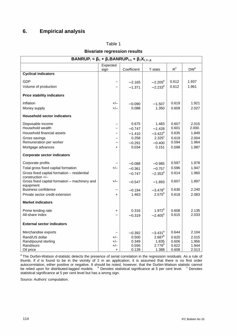
6. Empirical analysis

Table 1

Bivariate regression results

BANRUPt = β0 + β1BANRUPt-1 + β2Xi, t– p

Expected sign

Coefficient

T-stats

R2

DWa

Cyclical indicators GDP – –2.165 –2.205b 0.612 1.937

Volume of production – –1.371 –2.233b 0.612 1.961 Price stability indicators Inflation +/– –0.090 –1.507 0.619 1.921

Money supply +/– 0.088 1.350 0.609 2.027 Household sector indicators Disposable income – 0.675 1.483 0.607 2.015 Household wealth – –0.747 –1.428 0.601 2.000.

Household financial assets – –1.410 –3.422b 0.635 1.849

Gross savings – 0.258 2.325c 0.619 2.004 Remuneration per worker – –0.291 –0.400 0.594 1.964

Mortgage advances + 0.034 0.151 0.598 1.987 Corporate sector indicators Corporate profits – –0.088 –0.985 0.597 1.978

Total gross fixed capital formation +/– –0.361 –0.757 0.596 1.947

Gross fixed capital formation – residential construction +/–

–0.747 –2.353b 0.614 1.960

Gross fixed capital formation – machinery and equipment

+/– –0.547 –1.893 0.607 1.897

Business confidence – –0.194 –3.478b 0.636 2.240

Private sector credit extension + 1.463 2.575b 0.618 2.083 Market indicators Prime lending rate + 0.316 1.972b 0.608 2.135 All-share index – –0.319 –2.405b 0.615 2.033

External sector indicators Merchandise exports – –0.392 –3.431b 0.644 2.104

Rand/US dollar +/– 0.500 2.687b 0.620 2.015 Rand/pound sterling +/– 0.349 1.835 0.606 1.956 Rand/euro +/– 0.556 2.776b 0.622 1.944 Oil price + 0.139 1.388 0.608 2.013

a The Durbin-Watson d-statistic detects the presence of serial correlation in the regression residuals. As a rule of thumb, if d is found to be in the vicinity of 2 in an application, it is assumed that there is no first order autocorrelation, either positive or negative. It should be noted, however, that the Durbin-Watson statistic cannot be relied upon for distributed-lagged models. b Denotes statistical significance at 5 per cent level. c Denotes statistical significance at 5 per cent level but has a wrong sign.

Source: Authors’ computation.


6.1 Scenario analysis

Scenario analysis was done in order to measure the impact of various adverse macroeconomic events (shocks) on the dependent variable (bankruptcies). The historical approach for selecting scenarios was adopted.

Adverse changes (scenarios) in the shock variables and the period in which they occurred are presented in Annex 9, while Annex 10 provides a graphical illustration of the scenarios.

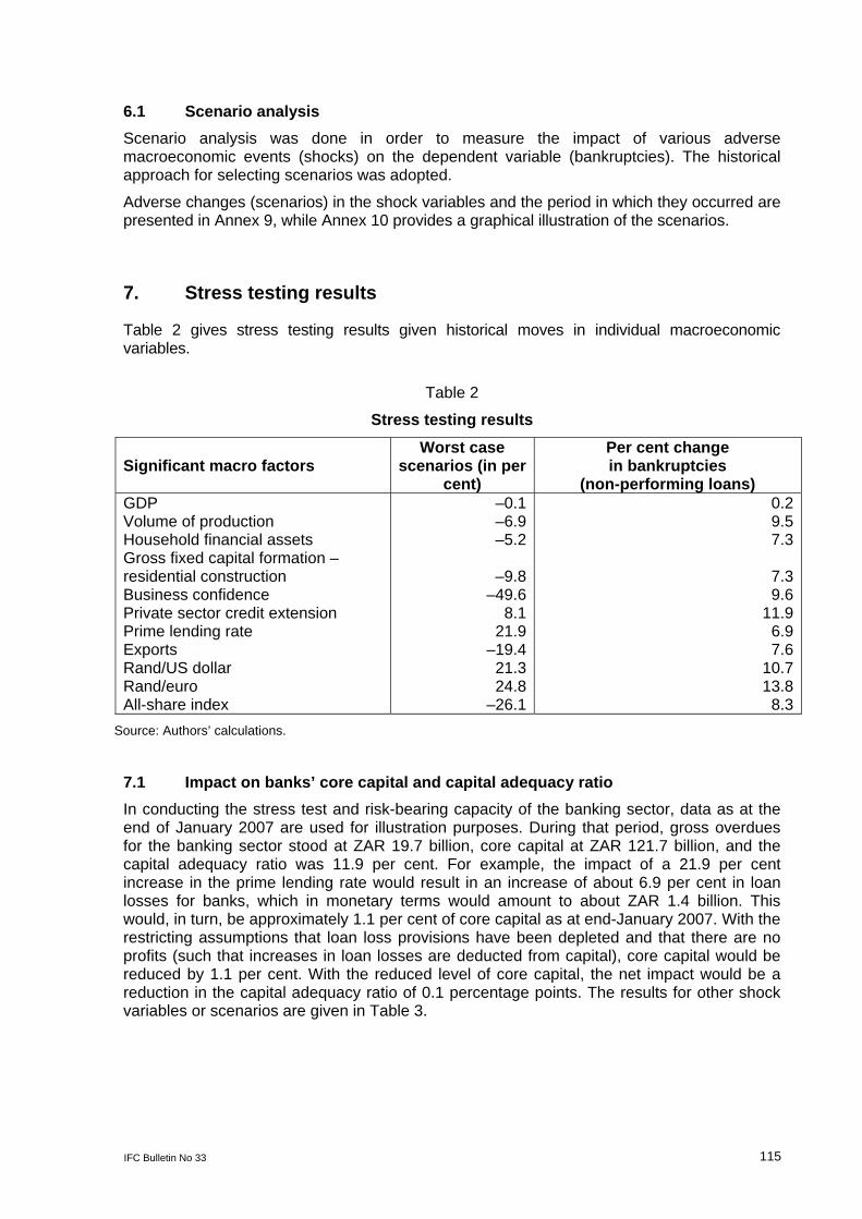
7. Stress testing results

Table 2 gives stress testing results given historical moves in individual macroeconomic variables.

Table 2

Stress testing results

Significant macro factors Worst case

scenarios (in per cent)

Per cent change in bankruptcies

(non-performing loans) GDP Volume of production Household financial assets Gross fixed capital formation – residential construction Business confidence Private sector credit extension Prime lending rate Exports Rand/US dollar Rand/euro All-share index

–0.1–6.9–5.2

–9.8–49.6

8.121.9

–19.421.324.8

–26.1

0.29.57.3

7.39.6

11.9 6.9

7.610.713.8 8.3

Source: Authors’ calculations.

7.1 Impact on banks’ core capital and capital adequacy ratio

In conducting the stress test and risk-bearing capacity of the banking sector, data as at the end of January 2007 are used for illustration purposes. During that period, gross overdues for the banking sector stood at ZAR 19.7 billion, core capital at ZAR 121.7 billion, and the capital adequacy ratio was 11.9 per cent. For example, the impact of a 21.9 per cent increase in the prime lending rate would result in an increase of about 6.9 per cent in loan losses for banks, which in monetary terms would amount to about ZAR 1.4 billion. This would, in turn, be approximately 1.1 per cent of core capital as at end-January 2007. With the restricting assumptions that loan loss provisions have been depleted and that there are no profits (such that increases in loan losses are deducted from capital), core capital would be reduced by 1.1 per cent. With the reduced level of core capital, the net impact would be a reduction in the capital adequacy ratio of 0.1 percentage points. The results for other shock variables or scenarios are given in Table 3.


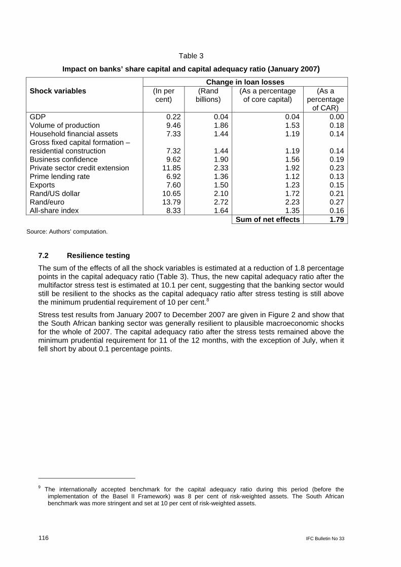
Table 3

Impact on banks’ share capital and capital adequacy ratio (January 2007)

Change in loan losses Shock variables (In per

cent) (Rand

billions) (As a percentage of core capital)

(As a percentage

of CAR) GDP Volume of production Household financial assets Gross fixed capital formation –residential construction Business confidence Private sector credit extension Prime lending rate Exports Rand/US dollar Rand/euro All-share index

0.229.467.33

7.329.62

11.856.927.60

10.6513.79

8.33

0.041.861.44

1.441.902.331.361.502.102.721.64

0.04 1.53 1.19

1.19 1.56 1.92 1.12 1.23 1.72 2.23 1.35

0.000.180.14

0.140.190.230.130.150.210.270.16

Sum of net effects 1.79


7.2 Resilience testing

The sum of the effects of all the shock variables is estimated at a reduction of 1.8 percentage points in the capital adequacy ratio (Table 3). Thus, the new capital adequacy ratio after the multifactor stress test is estimated at 10.1 per cent, suggesting that the banking sector would still be resilient to the shocks as the capital adequacy ratio after stress testing is still above the minimum prudential requirement of 10 per cent.8

Stress test results from January 2007 to December 2007 are given in Figure 2 and show that the South African banking sector was generally resilient to plausible macroeconomic shocks for the whole of 2007. The capital adequacy ratio after the stress tests remained above the minimum prudential requirement for 11 of the 12 months, with the exception of July, when it fell short by about 0.1 percentage points.

9 The internationally accepted benchmark for the capital adequacy ratio during this period (before the

implementation of the Basel II Framework) was 8 per cent of risk-weighted assets. The South African benchmark was more stringent and set at 10 per cent of risk-weighted assets.


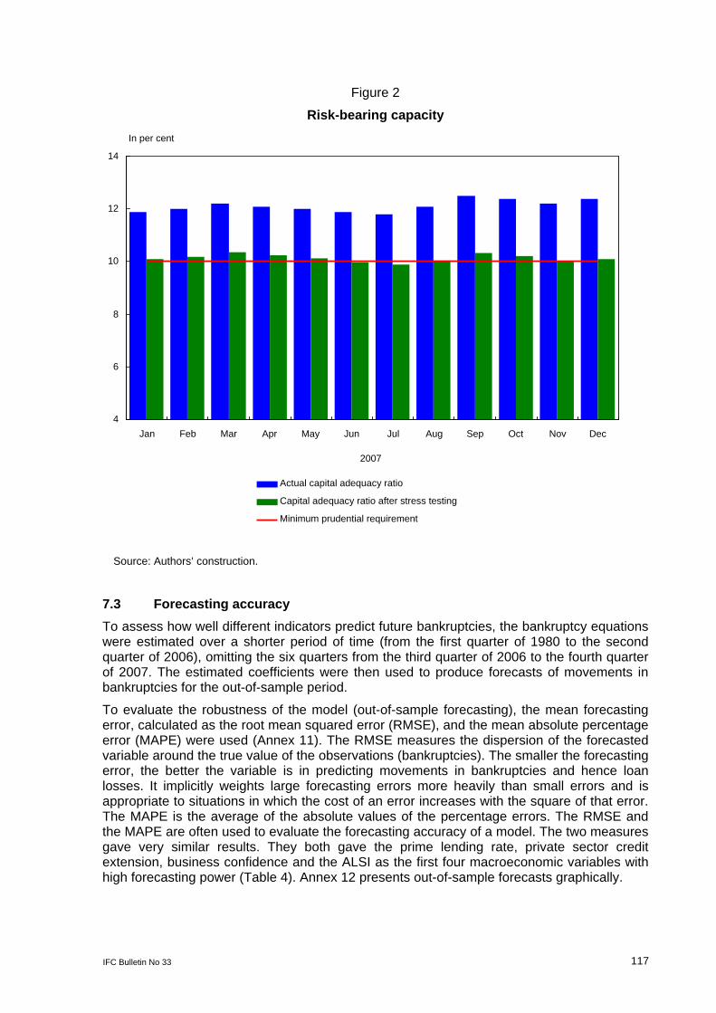
Figure 2

Risk-bearing capacity

Source: Authors’ construction.

2007

In per cent

Minimum prudential requirement

Capital adequacy ratio after stress testing

Actual capital adequacy ratio

DecNov OctSepAugJulJunMayApr Mar Feb Jan

14

12

10

8

6

4

7.3 Forecasting accuracy

To assess how well different indicators predict future bankruptcies, the bankruptcy equations were estimated over a shorter period of time (from the first quarter of 1980 to the second quarter of 2006), omitting the six quarters from the third quarter of 2006 to the fourth quarter of 2007. The estimated coefficients were then used to produce forecasts of movements in bankruptcies for the out-of-sample period.

To evaluate the robustness of the model (out-of-sample forecasting), the mean forecasting error, calculated as the root mean squared error (RMSE), and the mean absolute percentage error (MAPE) were used (Annex 11). The RMSE measures the dispersion of the forecasted variable around the true value of the observations (bankruptcies). The smaller the forecasting error, the better the variable is in predicting movements in bankruptcies and hence loan losses. It implicitly weights large forecasting errors more heavily than small errors and is appropriate to situations in which the cost of an error increases with the square of that error. The MAPE is the average of the absolute values of the percentage errors. The RMSE and the MAPE are often used to evaluate the forecasting accuracy of a model. The two measures gave very similar results. They both gave the prime lending rate, private sector credit extension, business confidence and the ALSI as the first four macroeconomic variables with high forecasting power (Table 4). Annex 12 presents out-of-sample forecasts graphically.


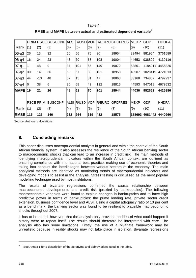
Table 4

RMSE and MAPE between actual and estimated dependent variable9

PRIM PSCE BUSCONF ALSI R/USD VOP R/EURO GFCFRES MEXP GDP HHDFA

Rank (1) (2) (3) (4) (5) (6) (7) (8) (9) (10) (11)

06-q3 26 13 32 50 56 75 90 18954 39494 881954 3761589

06-q4 16 24 23 43 70 68 108 19004 44653 938802 4139116

07-q1 1 48 9 37 101 65 149 19072 53801 1184911 4456826

07-q2 30 14 36 63 57 83 101 18958 48507 1028419 4721013

07-q3 44 -13 48 67 15 81 47 18863 33168 734867 4797237

07-q4 0 38 6 30 68 49 112 18815 44593 947018 4679532

MAPE 19 21 26 48 61 70 101 18944 44036 952662 4425886

PSCE PRIM BUSCONF ALSI R/USD VOP R/EURO GFCFRES MEXP GDP HHDFA

Rank (1) (2) (3) (4) (5) (6) (7) (8) (9) (10) (11)

RMSE 115 126 146 232 264 319 432 18575 188693 4081442 4440960

Source: Authors’ calculations.

8. Concluding remarks

This paper discusses macroprudential analysis in general and within the context of the South African financial system. It also assesses the resilience of the South African banking sector to macroeconomic shocks that can lead to an increase in credit risk. The main methods of identifying macroprudential indicators within the South African context are outlined as ensuring compliance with international best practice, making use of economic theories and taking into account the interlinkages between various sectors of the economy. The main analytical methods are identified as monitoring trends of macroprudential indicators and developing models to assist in the analysis. Stress testing is discussed as the most popular modelling technique used by most institutions.

The results of bivariate regressions confirmed the causal relationship between macroeconomic developments and credit risk (proxied by bankruptcies). The following macroeconomic variables were found to explain changes in bankruptcies and to have high predictive power in terms of bankruptcies: the prime lending rate, private sector credit extension, business confidence level and ALSI. Using a capital adequacy ratio of 10 per cent as a benchmark, the banking sector was found to be resilient to plausible macroeconomic shocks throughout 2007.

It has to be noted, however, that the analysis only provides an idea of what could happen if history were to repeat itself. The results should therefore be interpreted with care. The analysis also has some limitations. Firstly, the use of a bivariate framework may be unrealistic because in reality shocks may not take place in isolation. Bivariate regressions

9 See Annex 1 for a description of the acronyms and abbreviations used in the table.



may suffer from some flaws such as misspecification errors. Secondly, the use of a linear model to measure the impact of large shocks is restrictive because in reality shocks may have a non-linear impact. Thirdly, bankruptcies are a proxy for credit risk and thus an error-in-variables problem may be present. The analysis does, however, provide a foundation and backup for qualitative discussions that are always necessary when assessing the performance of the financial system.

Future research should focus on building rigorous models that can include both macroeconomic variables and FSIs as opposed to the bivariate approach used in this paper. This will allow for the simultaneous utilisation of all available information. Nevertheless, it is believed that the framework used does shed some light and is considered a reasonable starting point in attempting to assess the soundness of the South African financial system and its vulnerability to macroeconomic shocks.

Annex 1: Acronyms and abbreviations

ALSI All-share index BANRUP Bankruptcies BER Bureau for Economic Research BIS Bank for International Settlements BUSCONF Business confidence index CAMELS Capital adequacy, asset quality, management soundness, earnings,

liquidity and sensitivity to market risk CAR Capital adequacy requirements FSIs Financial soundness indicators FSAP Financial sector assessment programme FSSA Financial system stability assessment GDP Gross domestic product GFCFRES Gross fixed capital formation – residential construction HHDFA Household financial assets HHDW Household wealth IMF International Monetary Fund JSE Johannesburg Securities Exchange, SA LLP Loan loss provision MAPE Mean absolute percentage error MEXP Merchandise exports MORTADV Mortgage advances MPIs Macroprudential indicators NPLs Non-performing loans OLS Ordinary least squares OENB Oesterreichische Nationalbank PRIM Prime PSCEGDP Private sector credit extension as a percentage of GDP R/EURO Rand/euro exchange rate RMSE Root mean square error R/POUND Rand/pound sterling exchange rate R/USD Rand/US dollar exchange rate SARB South African Reserve Bank STATSSA Statistics South Africa VOP Volume of production ZAR South African rand


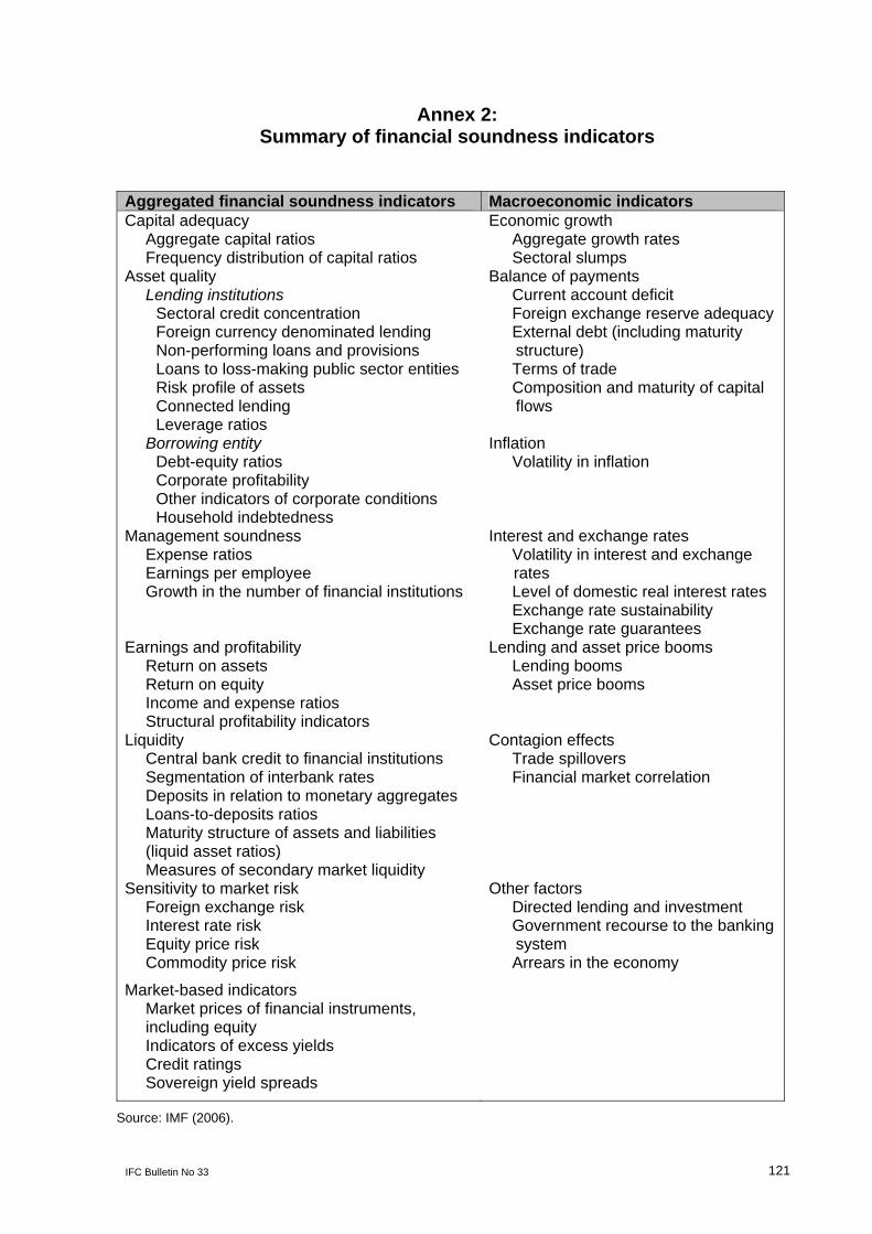
Annex 2: Summary of financial soundness indicators

Aggregated financial soundness indicators Macroeconomic indicators Capital adequacy Aggregate capital ratios Frequency distribution of capital ratios

Economic growth Aggregate growth rates Sectoral slumps

Asset quality Lending institutions Sectoral credit concentration Foreign currency denominated lending Non-performing loans and provisions Loans to loss-making public sector entities Risk profile of assets Connected lending Leverage ratios

Balance of payments Current account deficit Foreign exchange reserve adequacy External debt (including maturity structure) Terms of trade Composition and maturity of capital flows

Borrowing entity Debt-equity ratios Corporate profitability Other indicators of corporate conditions Household indebtedness

Inflation Volatility in inflation

Management soundness Expense ratios Earnings per employee Growth in the number of financial institutions

Interest and exchange rates Volatility in interest and exchange

rates Level of domestic real interest rates Exchange rate sustainability Exchange rate guarantees

Earnings and profitability Return on assets Return on equity Income and expense ratios Structural profitability indicators

Lending and asset price booms Lending booms Asset price booms

Liquidity Central bank credit to financial institutions Segmentation of interbank rates Deposits in relation to monetary aggregates Loans-to-deposits ratios Maturity structure of assets and liabilities

(liquid asset ratios) Measures of secondary market liquidity

Contagion effects Trade spillovers Financial market correlation

Sensitivity to market risk Foreign exchange risk Interest rate risk Equity price risk Commodity price risk

Other factors Directed lending and investment Government recourse to the banking system Arrears in the economy

Market-based indicators Market prices of financial instruments, including equity Indicators of excess yields Credit ratings Sovereign yield spreads

Source: IMF (2006).


Annex 3: Selected FSIs implied by economic

theories of financial stability

Theories (models) Main emphasis Recommended indicators

Debt and financial fragility Debt accumulation

Rising corporate and household debt accumulation relative to assets

Macroeconomic variables, real estate sector, economic growth, asset prices, income gearing, corporate and household debt, sectoral balance sheet, credit markets and investment trends

Monetarist approach Growth of monetary aggregates Monetary policy in general

Monetary aggregates, inflation, interest rates and exchange rates

Risks of bank runs Use of micro data on the banks’ balance sheets and profit and loss statements

Capital adequacy, overall interest rate margins, returns on assets or equity and banks’ assets, bank share prices, interbank claims and liabilities

Uncertainty, credit rationing and asymmetrical information

“Disaster myopia”

Emphasise and summarise other theories. Deviations from long-term averages are emphasised.

Loan spreads, rapid growth of markets, sectoral distribution of credit, bank capital ratios, net worth of customers

International aspects Vulnerability to external shocks Role of international capital flows

Foreign reserves, balance of payments transactions, foreign currency borrowing, capital inflows and contagion and commodity prices

Source: Authors’ construction based on Davis (1999 and 2001).


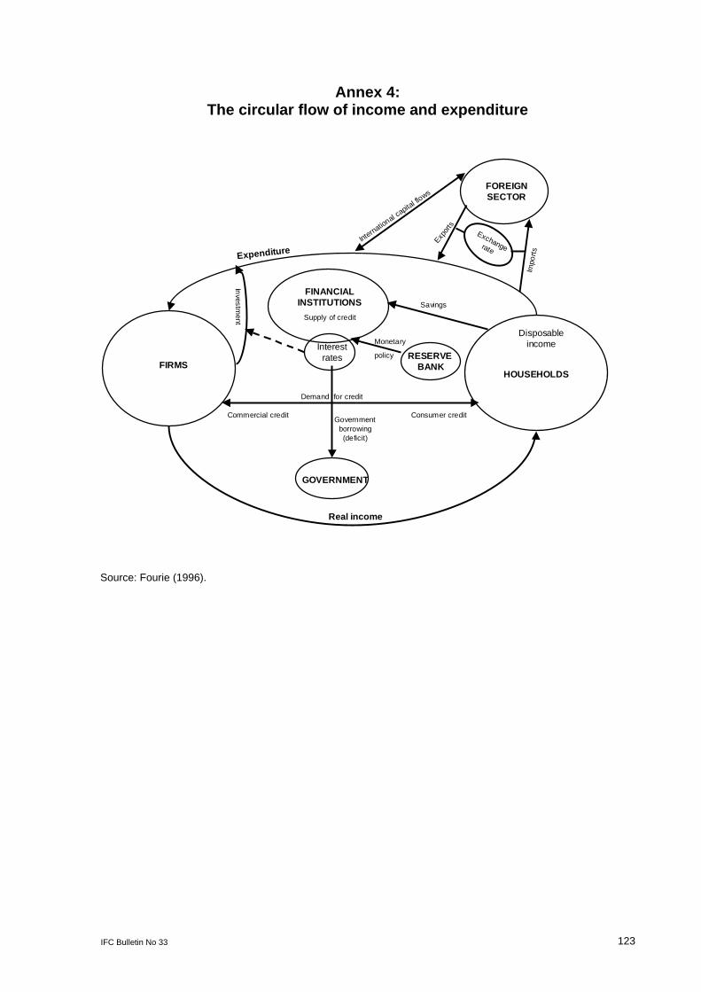
Annex 4: The circular flow of income and expenditure

RESERVE BANK

FINANCIAL INSTITUTIONS

Supply of credit

Interest rates

GOVERNMENT

FIRMSHOUSEHOLDS

Disposable income

Exchange rate

FOREIGN SECTOR

Monetary

policy

Demand for credit

Government borrowing (deficit)

Commercial credit Consumer credit

ExpenditureInternatio

nal capita

l flows

Expor

ts

Impo

rts

Savings

Real income

Inves tm

ent

Source: Fourie (1996).


Annex 5: Snapshot of macroprudential indicators

Financial services index Meana Thresholdb Actual

(Q1 2009) Signal issued

Retail banking confidence index Investment banking and specialized finance confidence index Investment managers confidence index Life insurance confidence index Financial services index

88 91

88 84 88

67 74

71 66 70

32 42

43 46 41

Yes Yes

Yes Yes Yes

Banking sector Mean Threshold Actual

(Feb 2009) Signal issued

Market share – top four banks, in per cent 83.9 84.3 84.4 No Concentration – H-index – Gini index Capital adequacy ratio Impaired advances (ZAR billions) Impaired advances as a percentage of total advances Total loans and advances (ZAR billions) Banking share prices (y-o-y), per cent change

0.186 83.4 12.6 71.6 3.1

2266 –24.0

0.188 83.8 12.2 89.8 3.9

2340 –30.9

0.190 84.0 13.0 106.1 4.6

2316 –23.9 (Mar 2009)

No No No Yes Yes No No

Insurance sector Mean Threshold Actual

(Q4 2008) Signal issued 5.1

Surrenders, in per cent Individual lapses, in per cent Number of policies (y-o-y), per cent change Insurance share prices (y-o-y), per cent change

21 36 5

2.3

27 47 –4

–20.5

13 59 6

–38.2 (March 2009)

No Yes No Yes

Corporate sector Mean Threshold Actual

(Mar 2009) Signal issued

Liquidations (y-o-y), per cent change Business confidence index

5.8 49

37.9 26

16.8 27 (Q1 2009)

No No

Household sector Mean Threshold Actual

(Q1 2009) Signal issued

Insolvencies (y-o-y), per cent change Consumer confidence index Credit card lending (y-o-y), per cent change

4.6 3.8

10.2

39.4 –6.2 16.6

20.8 (Feb 2009) 1.0

2.18 (Feb 2009)

No No No

Real estate sector Mean Threshold Actual

(Apr 2009) Signal issued

ABSA house price index (y-o-y), per cent change ABSA house price index (m-o-m), per cent change ABSA building cost index (y-o-y), per cent change Total mortgage advances (y-o-y), per cent change

12.7 0.92 12.0 18.6

2.6 0.09 19.3 22.5

–2.7 –0.38

5.6 (Q1 2009) 12.9 (Feb 2009)

Yes Yes No No

Real sector (annual growth rates) Mean Threshold Actual

(Mar 2009) Signal issued

Building plans passed Buildings completed Retail sales Wholesale trade sales Electric current generated New vehicle sales

11.4 14.9 6.1 5.7 2.6 5.2

–13.4 –8.3 1.5

–0.2 –1.6 –16.0

–36.2 –4.5 –5.1 –10.4 –7.7

40.2 (Apr 2009)

Yes No Yes Yes Yes Yes

a Data ranges for computing the mean are not the same for all indicators. b The benchmark (threshold) is calculated as the mean value of the indicator adjusted by the less favourable standard deviation. The actual value of the indicator is compared to the threshold value and is interpreted as giving a warning signal to vulnerability in the financial system if it crosses the threshold.



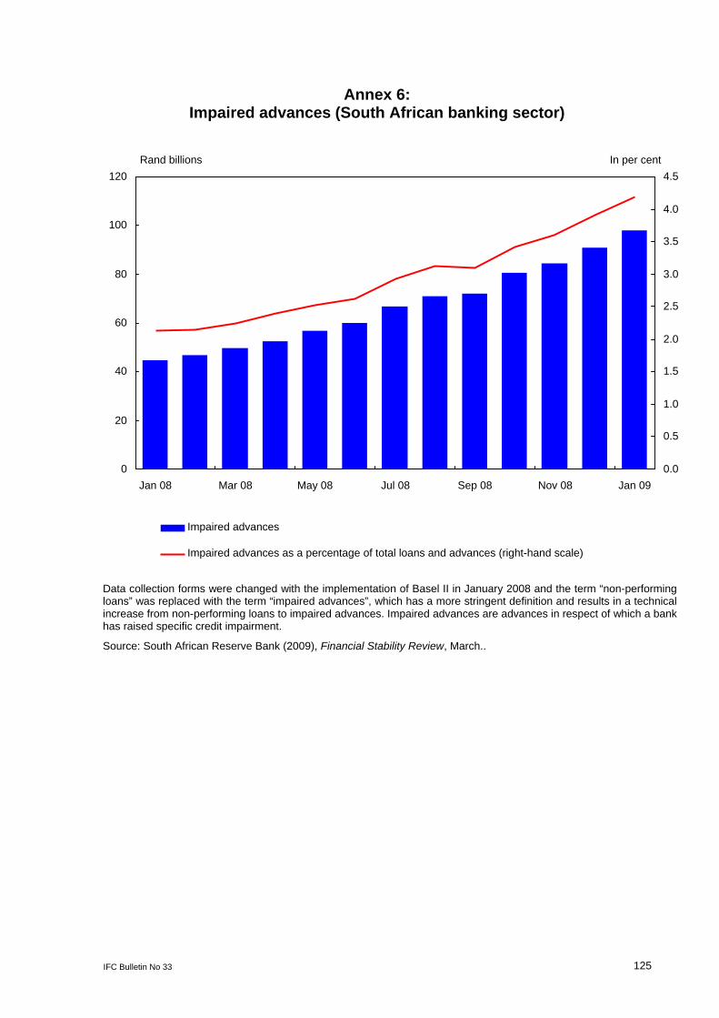
Annex 6: Impaired advances (South African banking sector)

In per centRand billions

Impaired advances as a percentage of total loans and advances (right-hand scale)

Impaired advances

4.5

4.0

3.5

3.0

2.5

2.0

1.5

1.0

0.5

0.0

Jan 09Nov 08 Sep 08Jul 08May 08Mar 08 Jan 08

120

100

80

60

40

20

0

Data collection forms were changed with the implementation of Basel II in January 2008 and the term “non-performing loans” was replaced with the term “impaired advances”, which has a more stringent definition and results in a technical increase from non-performing loans to impaired advances. Impaired advances are advances in respect of which a bank has raised specific credit impairment.

Source: South African Reserve Bank (2009), Financial Stability Review, March..


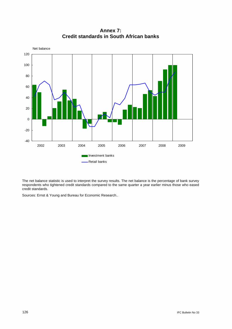
Annex 7: Credit standards in South African banks

-40

-20

0

20

40

60

80

100

120

Investment banks

Retail banks

Net balance

2002 2003 2004 2005 2006 2007 2008 2009

The net balance statistic is used to interpret the survey results. The net balance is the percentage of bank survey respondents who tightened credit standards compared to the same quarter a year earlier minus those who eased credit standards.

Sources: Ernst & Young and Bureau for Economic Research..


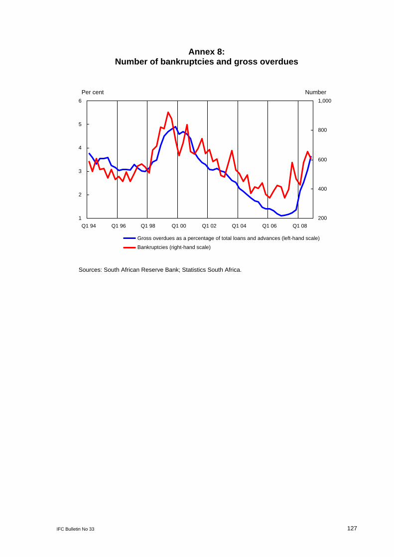
Annex 8: Number of bankruptcies and gross overdues

Number

Bankruptcies (right-hand scale)

Gross overdues as a percentage of total loans and advances (left-hand scale)

1,000

800

600

400

200

Q1 08 Q1 06Q1 04Q1 02Q1 00Q1 98 Q1 96

6 Per cent

5

4

3

2

1 Q1 94

Sources: South African Reserve Bank; Statistics South Africa.


Annex 9: Scenarios

Historical moves (shocks)

Shock variables

Period

Range

Per cent change

Rand/euro* 1985 – quarter 3 ZAR 1.49–ZAR 1.86 24.8 Rand/US dollar 1985 – quarter 3 ZAR 1.95–ZAR 2.35 20.3 Prime lending rate 1998 – quarter 2 18.25%–22.25% 21.9 Private sector credit extension 2003 – quarter 1 56.51%–61.07% of GDP 8.1 Volume of production 1989 – quarter 1 95.49–88.93 (index) –6.9 Business confidence index 1984 – quarter 3 46.00–23.00 –49.6 All-share index 1987 – quarter 4 36.64–27.08 –26.1

(Rand millions) GDP 1979 – quarter 2 44,592–44,552 –0.1 Merchandise exports 1979 – quarter 2 8,987–7,243 –19.4 Household financial assets 1998 – quarter 3 1,002,254–950,646 –5.2 Gross fixed capital formation – residential construction 1985 – quarter 1 21,610–19,544 –9.8

* The figures for the rand/euro exchange rate were calculated retrospectively by the South African Reserve Bank as the euro was only introduced in 2000.



Annex 10: Graphical illustration of scenarios

Source: South African Reserve Bank.


Annex 10: Graphical illustration of scenarios (cont)

Source: South African Reserve Bank.

-30

-20

-10

0

10

20

1980 1985 1990 1995 2000 2005

All-sh ar e in d ex Prime

28

8

12

16

20

24

1980 1985 1990 1995 2000 2005

-20

-10

0

10

20

30

1980 1985 1990 1995 2000 2005

Ra n d / e ur o

-20

-10

0

10

20

30

1980 1985 1990 1995 2000 2005

Rand/US dollar

-8

-4

0

4

8

12

1980 1985 1990 1995 2000 2005

Volu me o f p r od uct ion

% c h a n g e

% change% c h a n g e

% cha nge

% change

- 26,1

21,9

2 4,8 21,3

- 6,9

LSI

PRIM

R

A

/USDR/EU R O

VOP


Annex 11: The root mean squared error (RMSE) and the

mean absolute percentage error (MAPE)

RMSE =2

1

)ˆ(1

i

n

ii YY

n . . . . . . . . . . . . . . . . . (2)

MAPE =

i

ii

YYY ˆ

100 . . . . . . . . . . . . . . . . . (3)

Where n is the sample size,

Yi is the actual observation, and

Ŷi is the estimated value of Yi.


Annex 12 Out-of-sample forecasting

50

250

450

650

850

1,050

1,250

Q1 80 Q1 85 Q1 90 Q1 95 Q1 00 Q1 05


Source: Statistics South Africa; authors’ calculations.

Bankruptcies PSCE as per cent of GDP Prime R/euroR/US dollar ALSIVolume of production Business confidence index

Number

Actual bankruptcies

Out-of-sampleregion

References

Bell, J and D Pain (2000): “Leading indicator models of banking crises – a critical review”, Financial Stability Review, Bank of England, issue 9, 14 December.

Blaschke, W, M T Jones, G Majnoni and S M Peria (2001): “Stress testing of financial systems: an overview of issues, methodologies, and FSAP experience”, IMF Working Paper 01/88, Washington, DC, June.

Caruana, J (2007): “Macroprudential stress testing: reflections on current practices and future challenges”, remarks at a conference sponsored by the European Central Bank, Frankfurt am Main, 8 August.

Central Bank of Iceland (2008): Financial Stability, vol 4, May.

Committee on the Global Financial System (CGFS) (2000): Stress testing by large financial institutions: current practice and aggregation issues, Basel, April.

Davis, E P (1999): Financial data needs for macroprudential surveillance – what are the key indicators of risks to domestic financial stability?, Handbooks in Central Banking Lecture Series no 2, Centre for Central Banking Studies, Bank of England, May.

——— (2001): “A typology of financial stability”, Financial Stability Report 2, Oesterreichische Nationalbank.

Evans, O, A M Leone, M Gill and P Hilbers (2000): “Macroprudential indicators of financial system soundness”, IMF Occasional Paper no 192, April.

Fourie, F C v N (1996): How to think and reason in macroeconomics, Juta & Co Ltd.

Gujarati, D N (1995): Basic Econometrics, McGraw-Hill Inc, 1 September.

International Monetary Fund (IMF) (2006): Financial soundness indicators compilation guide, March.

Quantitative Micro Software, LLC (2007): EViews 6 User’s Guide II, 9 March.

Selialia, L F, K C Matlapeng and T T Mbeleki (2002): Macroprudential analysis of the South African financial system, South African Reserve Bank Working Paper, December.

Selialia, L F, P V Mabuza, K C Matlapeng and T T Mbeleki (2003): Effects of macroeconomic developments on credit risk of the South African banking sector: a stress testing approach, South African Reserve Bank Working Paper, June.

South African Reserve Bank (2009): Financial Stability Review, March.

Woolford, I (2001): “Macrofinancial stability and macroprudential analysis”, Reserve Bank Bulletin, Reserve Bank of New Zealand, vol 64, no 3, March, pp 29–43.


Macroprudential analysis of the financial system: the · PDF fileMacroprudential analysis of...

Documents

Transcript of Macroprudential analysis of the financial system: the · PDF fileMacroprudential analysis of...