Macroeconomics for small screens All files
38
Macroeconomics for small screens Abbreviations 11 GDP and circular flow 11.1 GDP (methods of calculation) 11.2 Relations between GDP and GNP 11.3 Circular flow 12 Employment, business cycle and growth 12.1 Business cycle 12.2 Unemployment 1 (types) 12.3 Unemployment 2 (impacts) 12.4 Investment demand 12.5 Aggregate demand (Keynes) 12.6 Aggregate demand and multiplier 12.7 Multiplier and accelerator 13 Money, interest and inflation 13.1 Money market 13.2 Inflation 1 (nature) 13.3 Inflation 2 (types) 13.4 Inflation 3 (impacts) 13.5 Deflation (characteristics) 13.6 Stagflation 13.7 Crowding-out effect 14 Fiscal policy and monetary policy 14.1 Objectives and policies 14.2 Fiscal policy 14.3 Laffer curve 14.4 Monetary policy
Transcript of Macroeconomics for small screens All files

Macroeconomics for small screens Abbreviations 11 GDP and circular flow
11.1 GDP (methods of calculation) 11.2 Relations between GDP and GNP 11.3 Circular flow 12 Employment, business cycle and growth
12.1 Business cycle 12.2 Unemployment 1 (types) 12.3 Unemployment 2 (impacts) 12.4 Investment demand 12.5 Aggregate demand (Keynes) 12.6 Aggregate demand and multiplier 12.7 Multiplier and accelerator 13 Money, interest and inflation
13.1 Money market 13.2 Inflation 1 (nature) 13.3 Inflation 2 (types) 13.4 Inflation 3 (impacts) 13.5 Deflation (characteristics) 13.6 Stagflation 13.7 Crowding-out effect 14 Fiscal policy and monetary policy
14.1 Objectives and policies 14.2 Fiscal policy 14.3 Laffer curve 14.4 Monetary policy

14.5 Liquidity trap 14.6 Phillips curve 14.7 Quantity theory of money 15 Foreign trade
15.1 Exchange rates 1 (flexible) 15.2 Exchange rates 2 (fixed) 15.3 Current account 16 Income distribution
16.1 Lorenz curve 1 (nature, form) 16.2 Lorenz curve 2 (redistribution) 16.3 Gini coefficient 17 Additional items
17.1 Economy and environment 17.2 Labour force 17.3 Paradox of thrift 17.4 Poverty (vicious circle) 17.5 Wealth (virtuous circle)
2019-05-01

Abbreviations macro
AD Aggegate demand AS Aggregate supply C Consumption D Demand G Government spending GDP Gross domestic product GNP Gross national product I Investment i or r Interest rates M Imports Q Quantity r or i Interest rates S Savings T Taxes X Exports Y National income, output
2019-05-01

2019-05-01
Expenditure
Output
Expenditure : C + I + G + (X-M)
Output: Sum of the value added of production
Income
Income: Wages + profits + interest + rent
Calculation of gross domestic product:

C G
DP
NI = Net income from abroad (from labour, from investments)
If NI > 0, then GDP < GNP (more income from abroad than to abroad) (>>> above)
If NI < 0, then GDP > GNP (less income from abroad than to abroad)
11.2 Relation between GDP and GNP
I
G
X - M
NI
GN
P
2019-05-01

2019-05-01
11.3 Circular flow
Households Firms
Income
Consumer expenditure (C)
Factors of production
+ Injections I,G,X - Withdrawels S,T,M
Goods and services

Economic activity
Time
3
12.1 Business cycle
1
2
Recovery
Boom
Recession
Depression
4
Phase Danger
1
2
3
4
Inflation
Unemployment
2019-05-01

2019-05-01
12.2 Unemployment 1(types)
Seasonal unemployment: regular during the year
Frictional unemployment: when joining the labour force or changing the job
Structural unemployment: due to changes in technology
Cyclical unemployment: during recessions

2019-05-01
- Loss of output
100
Output (index)
personal level - Frustration - Loss of skills
Impacts on the ...
12.3 Unemployment 2 (impacts)
macroeconomic level
with full employment
with unemployment
Gap = Loss of output
Time

i
12.4 Investment demand I D curve Change in i Shifting of D
D +
I
D
I
D
I D
I
D
I
i i
Negative relationship between i and I (ceteris paribus)
Movement along D (ceteris paribus): If i , then I If i , then I
D
-
Determinants: Growth (+) Recession (-) Optimism (+) Pessimism (-)

planned AD
Y
I + G
12.5 Aggregate demand (Keynes)
C
AD = Y
- AD = C + I + G (M - X = 0) - C = a + bY - I and G are not dependent on Y. - Y* = Equilibrium national income
AD
Y*
45o
2019-05-01

planned AD
Y
12.6 Aggregate demand and multiplier
AD = Y
AD1
45o
2019-05-01
Multiplier
Change in AD
Change in Y Change in AD
=
AD2
Y1 Y2 Change in Y

12.7 Multiplier and accelerator
Accelerator
Multiplier
Change in planned AD
Change in Y
Interaction
2019-05-01

2019-05-01
Money supply is determined by the central bank.
Money
Supply
Interest rate
13.1 Money market
Demand
Motives for demand: - Transactions - Precaution - Speculation The first two motives depend on the income, the third depends on the interest rate.

The two faces of inflation
Measuring inflation
- Consumer Price Index - Producer Price Index - GDP-Deflator
13.2 Inflation 1 (nature)
Value of money Price level
Price level
Time
Value of money
Time
2019-05-01

Types of inflation
Price level
13.3 Inflation 2 (types)
Demand-pull
Example: Consumption
Cost-push
Example: Wages
GDP
AS1
AS2 Price level
GDP
AS
AD AD1
AD2
2019-05-01
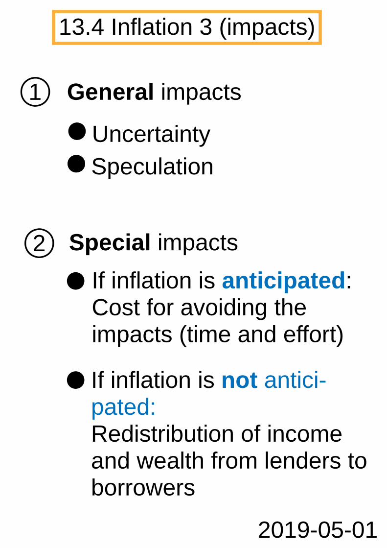
General impacts
If inflation is anticipated: Cost for avoiding the impacts (time and effort)
2019-05-01
13.4 Inflation 3 (impacts)
Uncertainty Speculation
Special impacts
If inflation is not antici- pated: Redistribution of income and wealth from lenders to borrowers
1
2
Time
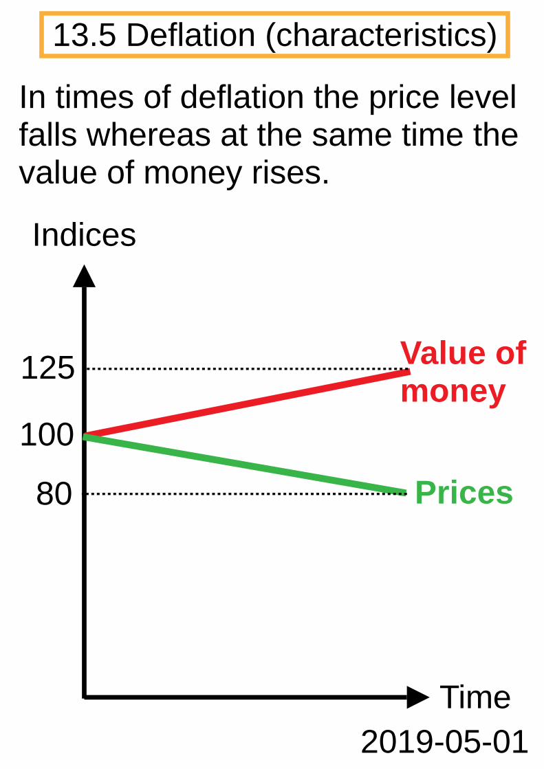
13.5 Deflation (characteristics)
2019-05-01
Value of money
Prices
In times of deflation the price level falls whereas at the same time the value of money rises.
Indices
100
125
80

Y
13.6 Stagflation
AS 1
Y 1
2019-05-01
In times of stagflation inflation and recession occur at the same time.
Example of a supply shock (oil crisis):
Price level (PL) AS 2
AD
Y 2
PL 2
PL 1
Y 1 = full employment

Private spending
2019-05-01
13.7 Crowding-out effect
Market for loans
Interest rate
Loans
An increase in government bor-rowing causes a reduction in pri-vate spending (C or I) due to an increase in interest rates.
Interest rate
Spending (C,I)
Supply
D1 D2

Objectives
Policies to target objectives
2019-05-01
14.1 Objectives and policies
- Price stability - Economic growth - Full employment
- Fiscal policy - Monetary policy

2019-05-01
AD1
Output
Price level
A recession is assumed. By using G and T, AD is changed.
14.2 Fiscal policy
AS
In this case, the fiscal policy is partially effective: Output and price level are increased. The fiscal policy is more effect- ive if the AS curve is less steep.
AD2

2019-05-01
In most cases, the peak will not be at the tax rate of 50 %. Neverthe-less, total tax revenue will be low if the tax rate is very low or very high.
0 %
Tax rate
Tota
l tax
rev
enue
14.3 Laffer curve
= peak, at the tax rate of 50 % 100 % 50 %

2019-05-01
Expansionary policy in a recession (Keynesian view)
14.4 Monetary policy
1r
AD (C+I+G+...) Investment Money market
Money
r
I
planned AD
Y
AD2
D
2
Y*2 Y*1
AD1
Supply

2019-05-01
very low r monetary policy ineffective
14.5 Liquidity trap
1 r
AD (C+I+G+...) Investment Money market
Money
r
I
planned AD
Y
D
2
Y*1=Y*2
AD1=AD2
Supply

Inflation (%)
2019-05-01
14.6 Phillips curve
Unemploy- ment (%) X
Y
The Phillips curve describes a negative relationship between inflation and unemployment.
Since the 1970s this relation- ship has not been constant any more. The curve is shifted from time to time.
X = unemployment / Y= inflation

2019-05-01
Classical and monetarist view: Monetary policy just changes the price level (and not other variables).
M * V = P * Q - M = Money supply - V = Velocity of circulation - P = Price level - Q = Output
14.7 Quantity theory of money
If V (pattern of payments) and Q (full employment) are constant, then it can be said:
A rise in M results in a proportional increase in P, e.g. more money, more inflation.

2019-05-01
Supply (£)
$ pe
r £
The rates are formed by market forces.
15.1 Exchange rates 1 (flexible)
and at a moment:
Time
$ pe
r £
Q (£)
Rates during a time period...
D (£)

2019-05-01
S (£)
$ pe
r £
The rates are formed by market forces within narrow
margins.
15.2 Exchange rates 2 (fixed)
and at a moment:
Time
$ pe
r £
Q (£)
Rates during a time period...
D (£)
Margins

2019-05-01
15.3 Current account
Current account
Trade in goods
Trade in services
Primary income *
Secondary income **
* Income from labour and financial capital
** Payments (without anything in return) (e.g. remittances by foreign workers)
The current account records a country's foreign exchange receipts and expenditures and is part of the balance of payments.

A Lorenz curve displays the income distribution or wealth distribution among households (HH) or persons (P).
2019-05-01
16.1 Lorenz curve 1 (nature, form)
HH/P (cumulative %) 0
100
100
Inco
me/
wea
lth
(cum
ulat
ive
%)
Lorenz curve
Diagonal of 45o = totally equal distribution

If a government redistributes income from rich to poor, e.g. by progressive taxes, the Lorenz curve shifts inwards (to the left).
2019-05-01
LC1
16.2 Lorenz curve 2 (redistribution)
Persons (cumulative %) 0
100
100
Inco
me
(cu-
m
ulat
ive
%)
Lorenz curve (LC)
LC2

Gini coefficient = Area between diagonal and LC Area ABC LC = Lorenz curve
2019-05-01 - 0 < Gini coeff. < 1
16.3 Gini coefficient
Persons (cumulative %)
100
- 100
Inco
me
(cu-
m
ulat
ive
%)
A B
C
LC
- The Gini coefficient is a measure of (in)equality in income.

2019-05-01
Factors of production
17.1 Economy and environment
Nature Nature Households Firms
Ene
rgy,
raw
m
ater
ials
Goods and services Waste
See also: Graham Dawson, Macroeconomics, Harlow 2006, 553

Unemployed
1 leaving labour force
17.2 Labour force
The labour force consists of em-ployed and unemployed persons.
Employed
3 2
getting employed again
5
1
2
3
4
4
5
changing the job
getting unemployed
entering labour force
2019-05-01

Equilibrium Y*: S = I
S,I
2019-05-01
17.3 Paradox of thrift
S
I
Y* Y
S1
I
Y*1 Y
More private saving does not result in higher S at Y*2
Paradox of thriftS2
Y*2
S,I

Low incomes
Low saving and investment
Source: Samuelson/Nordhaus: Economics, 18th ed, 583
17.4 Poverty (vicious circle)
Low capital accumulation
Low productivity
2019-05-01

High incomes
High saving and investment
17.5 Wealth (virtuous circle)
High capital accumulation
High productivity
2019-05-01