Macroeconomic determinants of cyclical variation in value, size and momentum premium in the UK

1

Macroeconomic Determinants of Cyclical Variations in Value, Size and

Momentum premium in the UK

Golam Sarwara,

Cesario Mateusa,

Natasa Todorovicb*

,

aUniveristy of Greenwich, London, UK

bThe Centre for Asset Management Research,

Cass Business School, City University, London, UK

This version: June 2014

Abstract

The paper examines the asymmetries in size, value and momentum premium over the

economic cycles in the UK and their macroeconomic determinants. Using Markov switching

approach we find clear evidence of cyclical variations of the three premiums, most noticeably

variations in size premium. We associate Markov switching regime 1 with economic upturn

and regime 2 with economic downturn as per OECD’s Composite Leading Indicator. The

macroeconomic indicators prompting such cyclicality the most are interest rates, term

structure and credit spread. The role of GDP growth, money supply and inflation is less

pronounced in our sample.

JEL classification: G11, E32

Key words: Size, Value and Momentum premium, Markov Switching, Macroeconomic

determinants

*Corresponding author. Tel.: +44 207 040 0120. E-mail addresses: [email protected] (Sarwar),

[email protected] (Mateus), [email protected] (Todorovic).

mailto:[email protected]

mailto:[email protected]

2

1. Introduction

Since Fama-French (1993) and Carhart (1997) related a small cap premium (small-minus-big

company returns (SMB)), value premium (high book to market minus low book to market

ratio stock returns (HML)) and momentum premium (winner minus loser stock returns) to

profitability, a vast body of literature that analyses determinants of those premiums has

emerged. While, for instance, DeBondt, Werner, & Thaler (1985) and Daniel, Hirshleifer, &

Subrahmanyam (1998) argue that the value premium arises due to the overreaction of

investors, a number of academic studies points that the value and size premium are proxies

for some non-diversifiable risks not captured by the standard CAPM model, such as risks

resulting from variations in macroeconomic factors (see Kelly, 2003; Liew & Vassalou,

2000; Petkova, 2006; Vassalou, 2003; Zhang, Hopkins, Satchell, & Schwob, 2009; Black and

McMillan, 2005; Gulen Xing, & Zhang, 2008, Kim et al., 2012 and Perez-Quiros &

Timmermann, 2000).

The literature on variety of macroeconomic sources that can cause asymmetries in expected

returns of value, small cap and winner portfolios over different phases of business cycle

focuses predominantly on the US market. It shows evidence that value portfolio returns

respond more to the changes of interest rates and money supply over the recessionary period

than expansionary period, supporting the asymmetric behaviour of returns over economic

phases (Black and McMillan, 2005). Three distinct sources, namely, costly reversibility,

operating leverage and financial leverage have been identified as the sources of relative

inflexibility of value firms in mitigating recessionary shocks. Hence these firms are riskier in

recessions leading to higher expected value premiums. First, costly reversibility implies the

higher cost of firms’ to scrap down the scale of productive assets than to expand. The value

firms want to disinvest more in economic downturn because the assets of value firms are less

profitable than growth firms; whereas this disinvesting is less important for growth firms

(Gulen et al., 2008). Since disinvesting is restricted by costly reversibility, the fundamentals

of value firms are affected more severely than the fundamentals of growth firms in economic

downturn when the credit market conditions are bad. In similar spirit, Gala (2005) argues that

investment irreversibility plays a vital role in explaining the size effects in stock returns and

their relation to risk and firms’ fundamentals. Second, when the demand of the product of a

firm decreases, the stock price of corresponding firm also decreases. This stock fall is in-line

with fall in book values and revenues falls relative to average values of the corresponding

3

firm. However, stock prices and revenues of value firms fall more relative to book values and

average level, respectively, the value firms ought to have higher operating leverage than

growth firms. Moreover, fixed costs of firms do not decrease proportionally with revenues in

economic downturn; and hence the earnings (revenue minus fixed and variable costs) will

decrease more than proportionally relative to revenues. This operating leverage mechanism

will have adverse effect on value firm by the negative aggregate shocks during economic

downturn as suggested by Gulen et al. (2008). Third, Livdan, Sapriza, & Zhang (2009) find

that value firms are characterized with higher financial leverage and investors require higher

expected returns to hold higher levered stocks during economic downturn when the value

firms are more exposed to the financial constraints.

Investigation into the small and large size firms reveals their sources of finance are different

implying they should be affected differently by credit market constraints. Perez-Quiros &

Timmermann (2000) argue that worsening credit market conditions in the economic

downturns have an adverse effect of on the small cap firms. Chan & Chen (1991) prove that

characteristics of a firm rather than its size matter for the size premium. Specifically, they

find a large proportion of marginal firms (with lower production efficiency and higher

financial leverage) in the small cap portfolio. Since marginal firms have lost market value

because of the poor performance, while having higher financial leverage and cash flow

problems; their price tends to be more sensitive to the economic states. Similar is confirmed

in the more recent study by Kim & Burnie (2002).

Firms with recent prior positive return (past winners) are likely to have had relatively more

positive growth rate shocks in comparison with the firms with recent prior negative return

(past losers), ceteris paribus. Johnson (2002) argues that stock price is a convex function of

expected growth, meaning that risk increases with growth rates and hence the stock returns

supposed to be more sensitive to the changes in expected growth during the higher expected

growth regime. In the case of positive risk premium - expected returns increase with growth

rates. Hence, past winners (past losers) tend to have higher (lower) growth rate changes in the

recent past, as well as higher (lower) subsequent expected returns (Kim, et al., 2012). Maio &

Santa-Clara (2011) identify three different sources of risk that might explain the momentum

anomalies: time varying betas, reinvestment risk and a common macroeconomic variable –

interest rates.

4

The focus of the attention in this search for macroeconomic determinants of varying value,

size and momentum premium over business cycles has by and large been on the US market.

Using size, value and momentum factors data from Gregory, Tharyan, & Christidis, (2013)

and Markov-switching model methodology, this paper seeks to contribute to the literature by

providing the first comprehensive study of the effect of a set of relevant macroeconomic

variables on those premiums in the UK market over varying economic regimes. The Markov

Switching framework of this study is closely related to Perez-Quiros & Timmermann (2000)

and Gulen et al. (2008), where the former investigate the systematic difference in variation of

size premium while the latter focuses on variations in value premium over the business

cycles. This study, however, scrutinizes the relative difference in change between size, value

and momentum premium over business cycles impacted by the variation in their

responsiveness to macroeconomic variables during different economic phases. In addition, to

the best of our knowledge, this is the first study that examines how all three equity premiums

are impacted by macroeconomic factors during the recent financial crisis in the UK.

We find that there is clear evidence of asymmetry in size, value and momentum premium

over the economic cycles in the UK. The most pronounced asymmetry is associated with size

premium. We document that credit market conditions have the greatest impact on the level of

the three premiums in both markets states in our sample.

The remainder of the paper is organised as follows: Section 2 outlines methodological

framework and describes the data; Section 3 discusses the findings before concluding in

Section 4.

2 Data and Methodology

2.1. Style Premiums

This study uses monthly UK market data from July’1982 to December’2012. The UK SMB,

HML and UMD factor data is from Gregory, Tharayan, and Christidis (2013)1, which is

comparable with the Fama-French’s and Carhart’s US equivalents. After sorting on market

capitalization, Gregory, Tharayan, and Christidis (2013) form two size groups of UK stocks,

namely ‘S’-small and ‘B’-big by using the median market capitalization of the largest 350

companies in the year ‘t’ as the size break point. Similarly, three book-to-market groups,

1 Downloadable from: http://business-school.exeter.ac.uk/research/areas/centres/xfi/research/famafrench/files/

http://business-school.exeter.ac.uk/research/areas/centres/xfi/research/famafrench/files/

5

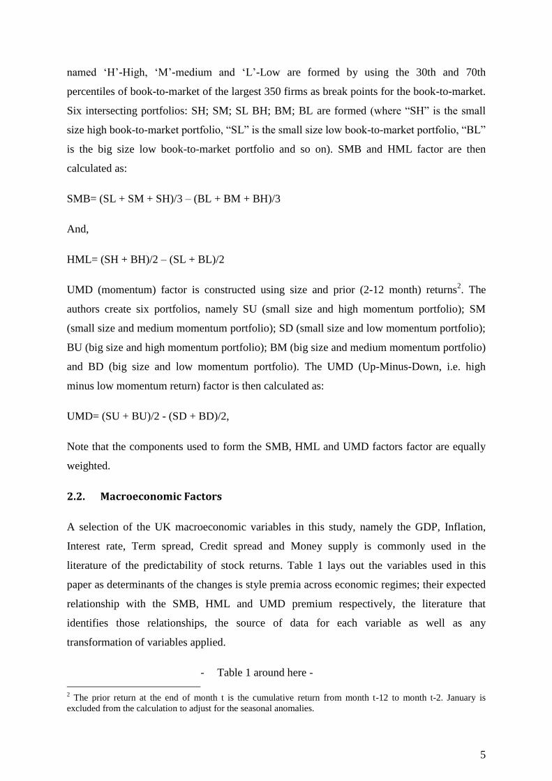
named ‘H’-High, ‘M’-medium and ‘L’-Low are formed by using the 30th and 70th

percentiles of book-to-market of the largest 350 firms as break points for the book-to-market.

Six intersecting portfolios: SH; SM; SL BH; BM; BL are formed (where “SH” is the small

size high book-to-market portfolio, “SL” is the small size low book-to-market portfolio, “BL”

is the big size low book-to-market portfolio and so on). SMB and HML factor are then

calculated as:

SMB= (SL + SM + SH)/3 – (BL + BM + BH)/3

And,

HML= (SH + BH)/2 – (SL + BL)/2

UMD (momentum) factor is constructed using size and prior (2-12 month) returns2. The

authors create six portfolios, namely SU (small size and high momentum portfolio); SM

(small size and medium momentum portfolio); SD (small size and low momentum portfolio);

BU (big size and high momentum portfolio); BM (big size and medium momentum portfolio)

and BD (big size and low momentum portfolio). The UMD (Up-Minus-Down, i.e. high

minus low momentum return) factor is then calculated as:

UMD= (SU + BU)/2 - (SD + BD)/2,

Note that the components used to form the SMB, HML and UMD factors factor are equally

weighted.

2.2. Macroeconomic Factors

A selection of the UK macroeconomic variables in this study, namely the GDP, Inflation,

Interest rate, Term spread, Credit spread and Money supply is commonly used in the

literature of the predictability of stock returns. Table 1 lays out the variables used in this

paper as determinants of the changes is style premia across economic regimes; their expected

relationship with the SMB, HML and UMD premium respectively, the literature that

identifies those relationships, the source of data for each variable as well as any

transformation of variables applied.

- Table 1 around here -

2 The prior return at the end of month t is the cumulative return from month t-12 to month t-2. January is

excluded from the calculation to adjust for the seasonal anomalies.

6

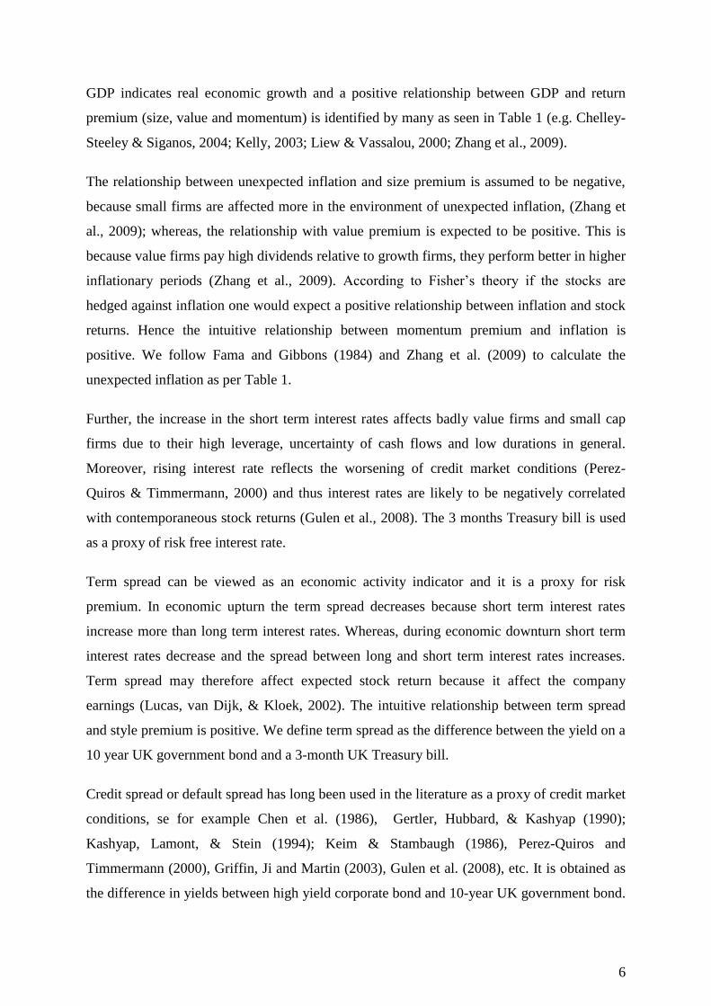
GDP indicates real economic growth and a positive relationship between GDP and return

premium (size, value and momentum) is identified by many as seen in Table 1 (e.g. Chelley-

Steeley & Siganos, 2004; Kelly, 2003; Liew & Vassalou, 2000; Zhang et al., 2009).

The relationship between unexpected inflation and size premium is assumed to be negative,

because small firms are affected more in the environment of unexpected inflation, (Zhang et

al., 2009); whereas, the relationship with value premium is expected to be positive. This is

because value firms pay high dividends relative to growth firms, they perform better in higher

inflationary periods (Zhang et al., 2009). According to Fisher’s theory if the stocks are

hedged against inflation one would expect a positive relationship between inflation and stock

returns. Hence the intuitive relationship between momentum premium and inflation is

positive. We follow Fama and Gibbons (1984) and Zhang et al. (2009) to calculate the

unexpected inflation as per Table 1.

Further, the increase in the short term interest rates affects badly value firms and small cap

firms due to their high leverage, uncertainty of cash flows and low durations in general.

Moreover, rising interest rate reflects the worsening of credit market conditions (Perez-

Quiros & Timmermann, 2000) and thus interest rates are likely to be negatively correlated

with contemporaneous stock returns (Gulen et al., 2008). The 3 months Treasury bill is used

as a proxy of risk free interest rate.

Term spread can be viewed as an economic activity indicator and it is a proxy for risk

premium. In economic upturn the term spread decreases because short term interest rates

increase more than long term interest rates. Whereas, during economic downturn short term

interest rates decrease and the spread between long and short term interest rates increases.

Term spread may therefore affect expected stock return because it affect the company

earnings (Lucas, van Dijk, & Kloek, 2002). The intuitive relationship between term spread

and style premium is positive. We define term spread as the difference between the yield on a

10 year UK government bond and a 3-month UK Treasury bill.

Credit spread or default spread has long been used in the literature as a proxy of credit market

conditions, se for example Chen et al. (1986), Gertler, Hubbard, & Kashyap (1990);

Kashyap, Lamont, & Stein (1994); Keim & Stambaugh (1986), Perez-Quiros and

Timmermann (2000), Griffin, Ji and Martin (2003), Gulen et al. (2008), etc. It is obtained as

the difference in yields between high yield corporate bond and 10-year UK government bond.

7

The intuitive relationship between credit spread with value and momentum premium is

positive. However, since small firms tend to be newcomers, poorly collateralized and don’t

have full access to the external financial markets, they have relatively stronger adverse effects

than large firms to the worsening credit market conditions. On average, an increase

(decrease) in the credit spread is expected to be associated with lower (higher) returns of

SMB. Moreover, asymmetries are expected for credit spread variables since firms are likely

to be more exposed to credit market conditions during recession (Perez-Quiros and

Timmermann, 2000)3.

Finally, the change in money supply proxies the liquidity changes and monetary policy

shocks (Gulen et al., 2008). It also measures the monetary policy shocks that might affect

aggregate economic conditions. Intuitively, changes in money supply effects the economic

conditions and investment premium as it indicates the credit market conditions. One could

expect a higher expected return for an increase in money supply. Small firms are found to be

strongly positively affected by lower money supply growth in the study of Perez-Quiros &

Timmermann (2000).

2.3 Econometric framework

We assume that, investors’ investment decisions differ across different economic regimes and

further, we assume the relationships of style factors (size, value and momentum) with

macroeconomic variables also vary. To characterize economic regimes in style investment

return, Perez-Quiros and Timmermann (2000), Guidolin and Timmermann (2008), Gulen,

Xing and Zhang (2008), Chung, Hung and Yeh (2012) adopt Markov Switching model. The

Markov Switching model, pioneered by Hamilton (1989), gained popularity for studying the

asymmetries across business cycle regimes, (Layton & Smith, 2007). This model allows

shifts from one regime to another and also gives probabilities of such transitions. It also takes

into account certain types of non-stationarity inherent in economic or financial time series

data that cannot be captured by classical linear models. These economic and financial time

series might obey to different economic regimes characterized by economic events such as

financial crisis (Jeanne and Masson, 2000) or abrupt economic policy changes (Hamilton,

3 Note that the high yield corporate bond data is not available for the UK market a period longer than 11 years.

To cover longer span of varying economic regimes, we resort to Moody’s US BAA corporate bond index as a

proxy for the UK data. The correlation coefficient Thomson Reuter UK Corporate Benchmark BBB (available

since April 2002) and Moody’s US BAA is 0.871085 over the 11 year period. Although there is a currency risk

involved in the proxy variable it can be minimized by hedging.

8

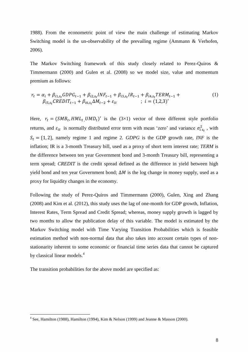
1988). From the econometric point of view the main challenge of estimating Markov

Switching model is the un-observability of the prevailing regime (Ammann & Verhofen,

2006).

The Markov Switching framework of this study closely related to Perez-Quiros &

Timmermann (2000) and Gulen et al. (2008) so we model size, value and momentum

premium as follows:

;

(1)

Here, is the (3×1) vector of three different style portfolio

returns, and is normally distributed error term with mean ‘zero’ and variance , with

, namely regime 1 and regime 2. GDPG is the GDP growth rate, INF is the

inflation; IR is a 3-month Treasury bill, used as a proxy of short term interest rate; TERM is

the difference between ten year Government bond and 3-month Treasury bill, representing a

term spread; CREDIT is the credit spread defined as the difference in yield between high

yield bond and ten year Government bond; is the log change in money supply, used as a

proxy for liquidity changes in the economy.

Following the study of Perez-Quiros and Timmermann (2000), Gulen, Xing and Zhang

(2008) and Kim et al. (2012), this study uses the lag of one-month for GDP growth, Inflation,

Interest Rates, Term Spread and Credit Spread; whereas, money supply growth is lagged by

two months to allow the publication delay of this variable. The model is estimated by the

Markov Switching model with Time Varying Transition Probabilities which is feasible

estimation method with non-normal data that also takes into account certain types of non-

stationarity inherent to some economic or financial time series data that cannot be captured

by classical linear models.4

The transition probabilities for the above model are specified as:

4 See, Hamilton (1988), Hamilton (1994), Kim & Nelson (1999) and Jeanne & Masson (2000).

9

= |

(2)

= | (3)

= |

(4)

= | (5)

Here, is the indicator of regimes for each of the style portfolio and is the cumulative

density function of standard normal variable. is the OECD’s Composite Leading

Indicator. Prior literature show that the transition probabilities between regimes are time

varying and depend on information variables such as economic leading indicator (see for e.g.

Filardo, 1994, Perez-Quiros & Timmermann, 2000, Gulen et al., 2008, Chung et al., 2012).

Layton (1998) argues that, such transition probabilities adjusted by information variables or

leading indicators provide very close correspondence to the business cycle chronology. To

ensure transition probabilities are accurately defined prior studies used logarithmic lag

difference of Composite Leading Indicators ( ). The Composite Leading Indicators

is designed to anticipate the turning point of economic cycles relative to trend and continue to

signal diverging growth patterns across the corresponding economy, (OECD, 2013).

2.4 Identification of the States

Figures 1, 2 and 3 provide an indication of the relation between the Markov switching states

the economic regimes. All three figures display the regime probabilities of being in low

volatile regime (regime 1) and high volatile regime (regime 2) for size, value and momentum

premium respectively at time t with the conditional information at time t-1. Here, P(S(t)=1)

and P(S(t)=2) are the probability of being in regime 1 and regime 2 respectively. The shaded

area is the economic downturn, measured by the OECD’s Composite Leading Indicator

(CLI). It can be observed that the predicted probabilities of being in the high volatile (low

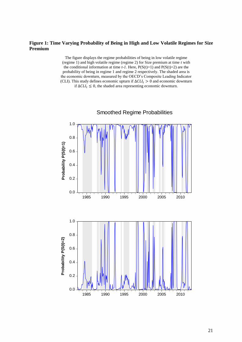
output) regime coincide with the recessionary period. Figure 1 illustrates that the smoothed

regime probabilities display clear time variation of small cap premium across the states of the

economy and the probabilities of being in regime 2 is quite high during the economic

10

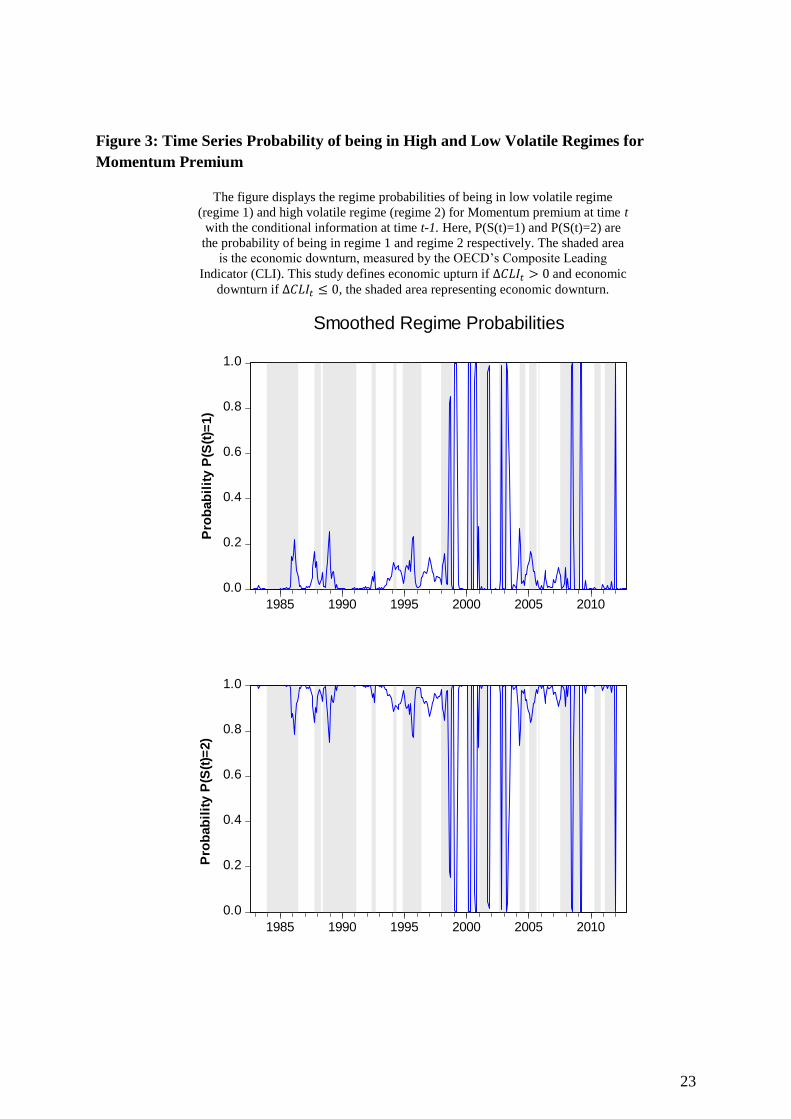
downturn. Figure 3 also displays the strong time variation of momentum premium across the

economic states but the probabilities of being in regime 2 is lower during the economic

downturn. This might imply the procyclical behaviour of momentum premium. In contrast,

there is no strong time variation across economic states for the value premium in Figure 2.

Most variation is observed at the start of 2001/02 around the dot com bubble burst. During

that time high probability of value premium being in regime 2 (downturn) is observed. These

results further support that the regime 1 is the state of economic upturn and regime 2 is state

of economic downturn.

Moreover, we find that that the regime 2 is associated with the high conditional volatility,

measured by conditional standard deviation reported in Table 3 for the size, value and

momentum premium. These findings are align with those of Schwert (1990), Hamilton and

Lin (1996), Gulen et al. (2008), Perez-Quiros & Timmermann (2000) and Kim et al. (2012).

Given this, it can be inferred that the regime 1 corresponds to economic upturn and regime 2

to the economic downturn, which are characterised by low and high volatilities respectively.

- Figure 1 around here –



3 Empirical findings

3.1 Descriptive Statistics

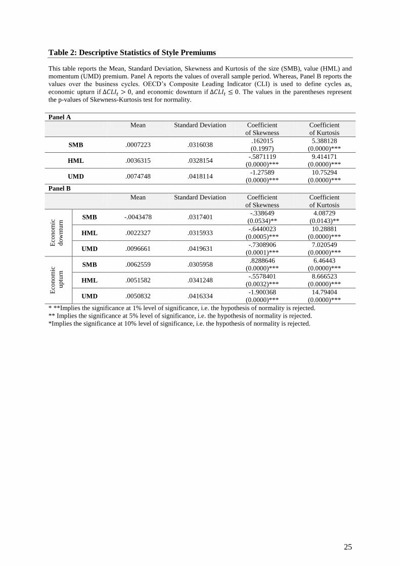
Table 2 presents the descriptive statistics (mean, standard deviation, skewness and kurtosis)

of the UK size, value and momentum premium in the overall sample period (Panel A) and in

economic downturns and upturns5 separately (Panel B). The mean returns of size, value and

momentum premium in the overall sample period reported in Panel A are 0.072%, 0.363%

and 0.747% with the standard deviation of 0.032, 0.033 and 0.418 respectively.


Panel B shows the domination of momentum premium with the mean return 0.967%

(standard deviation 0.042) in the economic downturn. In the good economic conditions the

5 As defined by OECD’s Composite Leading Indicator (CLI) described in section 2.3 of the paper

11

size premium is higher with mean return 0.626% along with standard deviation 0.031, which

is lower than other two premiums (value and momentum). This indicates that size stocks are

less risky with higher mean return in UK. Moreover, the size premium is larger in good

economic conditions than bad economic conditions which is similar to the findings of Kim &

Burnie (2002). Further, in both Panel A and Panel B, all but the SMB premium are

significantly negatively skewed with kurtosis higher than 3 in all the cases, implying non-

normal distribution of the three premia.

3.2 Markov Switching Model Results

Table 3 reports the parameter estimation of the equation (1) by the Markov switching model.

The constant term in regime 2 is lower than those of regime 1 universally for all the

style premiums, indicating lower expected value of the SMB, HML and UMD after adjusting

for the macroeconomic risk factors in the regime 2 then in regime 1. Except for the size

premium in regime 1, all of the constant terms are significant across the regimes. The highest

constant is the one associated with the momentum premium in both regimes. Furthermore,

while all three constants decrease when we move from regime 1 to regime 2, the greatest

change in the magnitude of the constant is associated with value premium (21.681%). This

evidence indicates that size, value and momentum premium reacts more to the negative than

positive shocks as the absolute value of premiums is larger in the economic downturn.

The magnitudes (in absolute terms) of most of the coefficients of macroeconomic variables

are higher during economic downturn than economic upturn suggesting that, investors require

greater compensation for higher macroeconomic risk (Black and McMillan, 2005). This is

most evident for the value premium, where all the coefficients are higher during economic

downturn, hinting that investors require additional compensation for holding the extreme

book-to-market portfolio. The magnitude of responsiveness of the size and momentum

premium to changes in regimes is comparatively lower.


The results in Table 3 reveal the positive relationship between GDP growth and all the

premia in regime 1, but negative in regime 2, since firms with small capitalization, high

book-to-market ratios and past winners are more likely to be distressed and vulnerable during

12

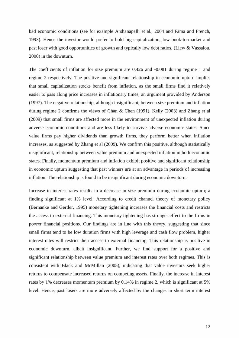
bad economic conditions (see for example Arshanapalli et al., 2004 and Fama and French,

1993). Hence the investor would prefer to hold big capitalization, low book-to-market and

past loser with good opportunities of growth and typically low debt ratios, (Liew & Vassalou,

2000) in the downturn.

The coefficients of inflation for size premium are 0.426 and -0.081 during regime 1 and

regime 2 respectively. The positive and significant relationship in economic upturn implies

that small capitalization stocks benefit from inflation, as the small firms find it relatively

easier to pass along price increases in inflationary times, an argument provided by Anderson

(1997). The negative relationship, although insignificant, between size premium and inflation

during regime 2 confirms the views of Chan & Chen (1991), Kelly (2003) and Zhang et al

(2009) that small firms are affected more in the environment of unexpected inflation during

adverse economic conditions and are less likely to survive adverse economic states. Since

value firms pay higher dividends than growth firms, they perform better when inflation

increases, as suggested by Zhang et al (2009). We confirm this positive, although statistically

insignificant, relationship between value premium and unexpected inflation in both economic

states. Finally, momentum premium and inflation exhibit positive and significant relationship

in economic upturn suggesting that past winners are at an advantage in periods of increasing

inflation. The relationship is found to be insignificant during economic downturn.

Increase in interest rates results in a decrease in size premium during economic upturn; a

finding significant at 1% level. According to credit channel theory of monetary policy

(Bernanke and Gertler, 1995) monetary tightening increases the financial costs and restricts

the access to external financing. This monetary tightening has stronger effect to the firms in

poorer financial positions. Our findings are in line with this theory, suggesting that since

small firms tend to be low duration firms with high leverage and cash flow problem, higher

interest rates will restrict their access to external financing. This relationship is positive in

economic downturn, albeit insignificant. Further, we find support for a positive and

significant relationship between value premium and interest rates over both regimes. This is

consistent with Black and McMillan (2005), indicating that value investors seek higher

returns to compensate increased returns on competing assets. Finally, the increase in interest

rates by 1% decreases momentum premium by 0.14% in regime 2, which is significant at 5%

level. Hence, past losers are more adversely affected by the changes in short term interest

13

rates in economic downturns than past winners. Although similar relationship is found in

regime 1, the coefficient is insignificant.

The relationship between term spread and size and value premium respectively exhibits

asymmetries in our findings over economic regimes. Aretz, Bartram & Pope (2010) argue

that shocks to term structure will have greater effect on larger firms than on the smaller ones

and hence a positive relationship is expected between term spread and size premium and our

results confirm this view in economic downturn. However, in the upmarket the opposite is

observed. Further, similar to Gregory, Harris, & Michou (2003), we find that during

upmarket a steepening in the yield curve has greater positive effect on value premium.

However, this effect is found to be negative during economic downmarket where the spread

is larger. Moreover, the significant negative relationship between term spread and momentum

premium indicates that the past losers benefit from the steepening of yield curve both in

economic upturn and downturn.

Credit (default or ‘quality’) spread is expected to show the evidence of asymmetry in up and

downturn since the small firms with low collateral are likely to more exposed to bankruptcy

risk during economic downturn (Perez-Quiros & Timmermann, 2000). We document a

significant positive relationship between credit spread and size premium in economic upturn.

This finding coincide with the findings of Fama and French (1988); Fama and French (1989).

In economic downturn however, that relationship is insignificant. The opposite is observed

for the momentum premium. During economic upturn the coefficient of credit spread is

negative and positive during economic upturn, indicating that past losers enjoy higher return

than past winners during economic upturn but past winner enjoy higher return during

economic downturn.

An increase in credit spread commonly interpreted as a sign of worsening credit market

conditions. One would expect positive relationship between credit spread and value premium

on average and we find evidence that corroborates this in both regimes. The magnitude (6.64)

of credit spread is higher in economic downturn indicates that value firms respond more to

increase in credit spread during bad economic conditions.

During an economic upturn, money supply appears not to be related to size, value and

momentum premiums, as all coefficients are insignificant at any conventional level. Similar

is reported by Black & McMillan (2005). During economic downturn the coefficients are

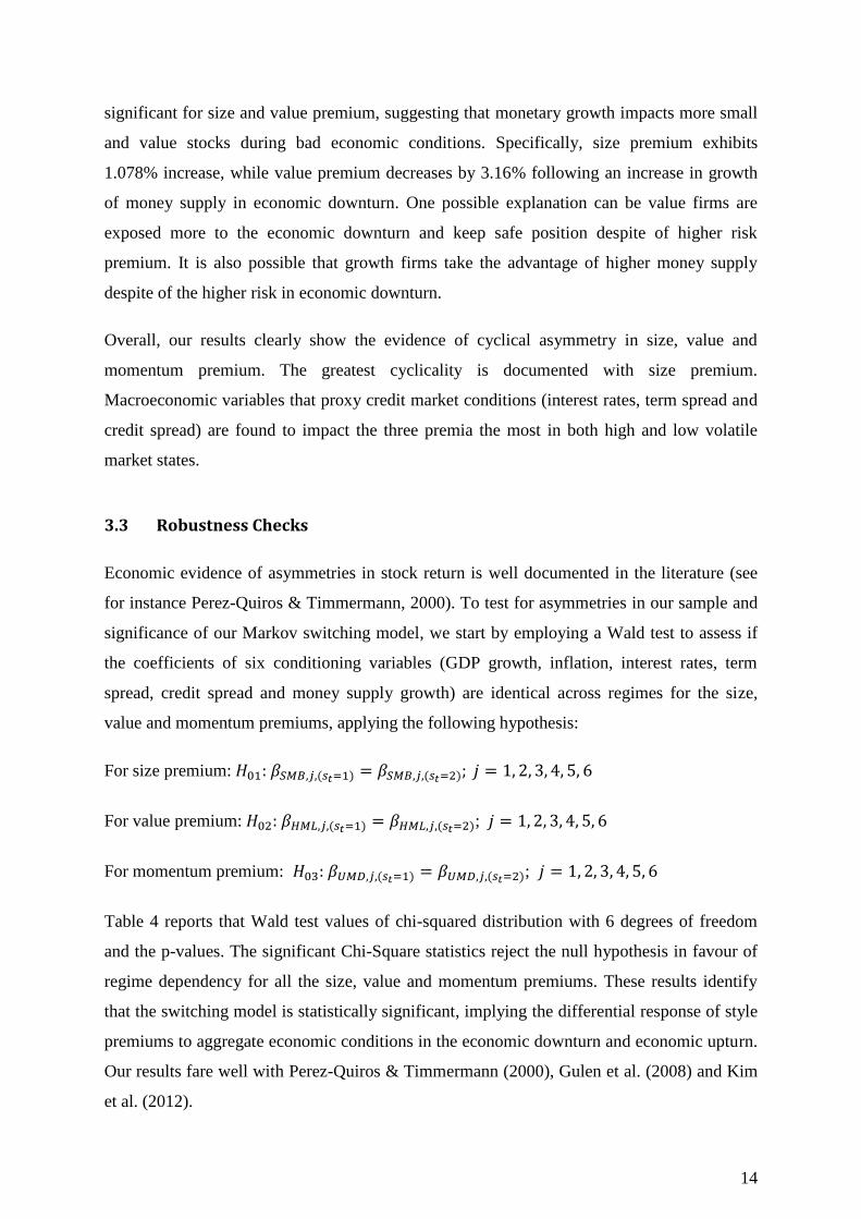
14

significant for size and value premium, suggesting that monetary growth impacts more small

and value stocks during bad economic conditions. Specifically, size premium exhibits

1.078% increase, while value premium decreases by 3.16% following an increase in growth

of money supply in economic downturn. One possible explanation can be value firms are

exposed more to the economic downturn and keep safe position despite of higher risk

premium. It is also possible that growth firms take the advantage of higher money supply

despite of the higher risk in economic downturn.

Overall, our results clearly show the evidence of cyclical asymmetry in size, value and

momentum premium. The greatest cyclicality is documented with size premium.

Macroeconomic variables that proxy credit market conditions (interest rates, term spread and

credit spread) are found to impact the three premia the most in both high and low volatile

market states.

3.3 Robustness Checks

Economic evidence of asymmetries in stock return is well documented in the literature (see

for instance Perez-Quiros & Timmermann, 2000). To test for asymmetries in our sample and

significance of our Markov switching model, we start by employing a Wald test to assess if

the coefficients of six conditioning variables (GDP growth, inflation, interest rates, term

spread, credit spread and money supply growth) are identical across regimes for the size,

value and momentum premiums, applying the following hypothesis:

For size premium:

For value premium: ;

For momentum premium: ;

Table 4 reports that Wald test values of chi-squared distribution with 6 degrees of freedom

and the p-values. The significant Chi-Square statistics reject the null hypothesis in favour of

regime dependency for all the size, value and momentum premiums. These results identify

that the switching model is statistically significant, implying the differential response of style

premiums to aggregate economic conditions in the economic downturn and economic upturn.

Our results fare well with Perez-Quiros & Timmermann (2000), Gulen et al. (2008) and Kim

et al. (2012).

15


To identify the significance of regressors in the model, the likelihood ratio test for redundant

variables is performed. Likelihood ratio rest is being performed under the null

hypothesis ; to identify the significance of each

regressor, namely GDP growth, inflation, interest rates, term spread, credit spread and money

supply growth. Table 5 reports the likelihood ratio test of redundant variables for the

estimated Time Varying Markov Switching model.


With the exception of GDP growth in determining the size premium, the likelihood ratio test

is significant for all of the regressors in size, value and momentum premiums. These results

corroborate the significant impact our chosen macroeconomic variables have on the three

premiums.

4 Summary and conclusions

This paper sheds light whether any asymmetries can be found in the UK size, value and

momentum premium as well as identifying the main drivers of these premiums in varying

market conditions. We focus on UK SMB, HML and UMD factors defined by Gregory,

Tharayan, and Christidis (2013) in the period January 1982 to December 2012. Employing

Markov switching methodology, we find evidence in strong support of asymmetry in

premiums across different Markov switching regimes. Our analysis of regimes related to

OECD’s Composite Leading Indicator prompts us to conclude that Markov switching regime

1, associated with lower conditional volatility coincides by and large with economic upturns

and vice versa for regime 2. We find that all three premiums vary across regimes but that

most asymmetries are observed in the size premium.

Following the US literature, we test whether GDP growth, inflation, interest rates, term

structure, credit spread and money supply are valid determinants of those cyclical variations

in UK equity return premiums. We corroborate findings from the US markets in that

macroeconomic factors are drivers of equity premiums in both economic upturn and

downturn. The strongest impact on size, value and momentum premium have variables that

proxy credit market conditions, namely interest rates, term structure and credit spread.

16

Finally, to test the significance of our Markov Switching model, we apply the Wald test and

redundant variable test (Likelihood Ratio Test). Walt test shows that the intercept and slope

of the Markov Switching model are regime dependent and hence there is differential response

of style premiums in upturn and downturn. Given the Likelihood Ratio Test, only GDP

growth used as the determinant surfaces as insignificant regressor in our model, with all the

other macroeconomic variables across the three premiums being deemed as significant ones,

at least at the 10% level.

This paper can be extended following Clare, Sapuric and Todorovic (2010) and Ammann &

Verhofen (2006). Specifically, multi-style rotation strategies, highly applicable particularly

among hedge fund investors can be deployed in high and low volatility regimes using

forecasting models based on macroeconomic variables suggested in this paper.

17

References

Ammann, M., & Verhofen, M. (2006). The Effect of Market Regimes on Style Allocation.

Financial Markets and Portfolio Management, 20(3), 309–337.

Anderson, R. (1997). A Large versus Small Capitalization Relative Performance Model. In

Market Timing Models. Burr Ridge: Irwin Professional Publishing.

Aretz, K., Bartram, S. M., & Pope, P. F. (2010). Macroeconomic Risks and Characteristic-

Based Factor Models. Journal of Banking & Finance, 34(6), 1383–1399.

Arshanapalli, B. G., D’Ouville, E. L., & Nelson, W. B. (2004). Are Size, Value, and

Momentum Related to Recession Risk? The Journal of Investing, 13(4), 83–87.

doi:10.3905/joi.2004.450760

Bernanke, B. S., & Gertler, M. (1995). Inside the Black Box: The Credit Channel of

Monetary Policy Transmission. Journal of Economic Perspectives, 9, 27–48.

Black, A. J., & McMillan, D. G. (2005). Value and growth stocks and cyclical asymmetries.

Journal of Asset Management, 6(2), 104–116. doi:10.1057/palgrave.jam.2240169

Carhart, M. (1997). On Persistence of Mutual Fund Performance. Journal of Finance, 52, 57–

82.

Chan, K. C., & Chen, N. (1991). Structural and Return Characteristics of Small and Large

Firms. The Journal of Finance, 46(4), 1467–1484.

Chelley-steeley, P., & Siganos, A. (2004). Momentum Profits and Macroeconomic Factors.

Applied Economics Letters, 11(7), 433–436. doi:10.1080/1350485042000191719

Chen, N. F., Roll, R., & Ross, S. A. (1986). Economic Forces and the Stock Market. Journal

of Business, 59(3), 383–403.

Chordia, T., & Shivakumar, L. (2002). Momentum , Business Cycle , and Time-varying.

Journal of Finance, 57(2), 985–1019.

Chung, S., Hung, C., & Yeh, C. (2012). When Does Investor Sentiment Predict Stock

Returns? Journal of Empirical Finance, 19(2), 217–240.

Daniel, K., Hirshleifer, D., & Subrahmanyam, A. (1998). Investor Psychology and Security

Market Under- and Overreaction. Journal of Finance, 53(6), 1839–1885.

DeBondt, M., W. F., & Thaler, R. (1985). Does the Stock Market Overreact? Journal of

Finance, 40, 793–805.

Fama, E. F., & French, K. R. (1988). Dividend Yields and Expected Stock Returns. Journal

of Financial Economics, 22(1), 3–25.

18

Fama, E. F., & French, K. R. (1989). Business Conditions and Expected Returns on Stocks

and Bonds. Journal of Financial Economics, 25(1), 23–49.

Fama, E., & French, K. (1993). Common Risk Factors in the Returns on Stocks and Bonds.

Journal of Financial Economics, 33(1), 3–56.

Fama, E., & Gibbons, M. (1984). A Comparison of Inflation Forecasts. Journal of Monetary

Economics, 13, 327–348.

Filardo, A. (1994). Business-Cycle Phases and Their Transitional Dynamics. Journal of

Business & Economic Statistics, 12(3), 299–308.

Gala, V. D. (2005). Investment and Returns. Working Paper, University of Chicago.

Gertler, M., Hubbard, R. G., & Kashyap, A. (1990). Interest Rate Spreads, Credit Constraints,

and Investment Fluctuations: an Empirical Investigation. Financial Markets and

Financial Crises, 11–32.

Gregory, A., Harris, R., & Michou, M. (2003). Contrarian Investment and Macroeconomic

Risk. Journal of Business Finance and Accounting, 30(1 & 2), 213–255.

Gregory, A., Tharyan, R., & Christidis, A. (2013). Constructing and Testing Alternative

Versions of the Fama–French and Carhart Models in the UK. Journal of Business

Finance & Accounting, 40(1&2), 172–214. doi:10.1111/jbfa.12006

Griffin, J., Ji, X., & Martin, J. (2003). Momentum Investing and Business Cycle Risk :

Evidence from Pole to Pole. The Journal of Finance, 58(6), 2515–2547.

Guidolin, M., & Timmermann, A. (2008). Size and value anomalies under regime shifts.

Journal of Financial Econometrics, 6(1), 1–48.

Gulen, H., Xing, Y., & Zhang, L. (2008). Value versus Growth : Time-Varying Expected

Stock Returns. Financial Management, 40(2), 381–407.

Hahn, J., & Lee, H. (2006). Yield spreads as Alternative Risk Factors for Size and Book-to-

Market. Journal of Financial and Quantitative Analysis, 41(2), 245–269.

Hamilton, J. (1989). A New Approach to the Economic Analysis of Nonstationary Time

Series and the Business Cycle. Econometrica, 57(2), 357–384.

Hamilton, J. D. (1988). Rational-Expectations Econometric Analysis of Changes in Regime:

an Investigation of the Term Structure of Interest Rates. Journal of Economic Dynamics

and Control, 12, 385–423.

Hamilton, J. D. (1994). Time Series Analysis. Princeton: Princeton University Press.

Hamilton, J., & Lin, G. (1996). Stock Market Volatility and the Business Cycle. Journal of

Applied Econometrics, 11, 573–593.

19

Jeanne, O., & Masson, P. (2000). Currency Crises, Sunspots, and Markov-Switching

Regimes. Journal of International Economics, 50, 327–350.

Johnson, T. C. (2002). Rational Momentum Effects. Journal of Finance, 57(2), 585–608.

Kashyap, A. K., Lamont, O. A., & Stein, J. C. (1994). Credit conditions and the cyclical

behavior of inventories. The Quarterly Journal of Economics, 109(3), 565–592.

Keim, D. B., & Stambaugh, R. F. (1986). Predicting Returns in the Stock and Bond Markets.

Journal of Financial Economics, 17(2), 357–390.

Kelly, P. (2003). Real and Inflationary Macroeconomic Risk in the Fama and French Size

and Book-to-Market Portfolio. EFMA 2003 Helsinki Meetings, (October).

Kim, C., & Nelson, C. R. (1999). State-Space Models with Regime Switching. Cambridge,

Massachusetts: MIT Press.

Kim, D., Roh, T., Min, B., & Byun, S. (2012). Time-Varying Expected Momentum Profits.

Working Paper Series, Available at SSRN 2336144.

Kim, M., & Burnie, D. (2002). The Firm Size Effect and the Economic Cycle. Journal of

Financial Research, 40(1), 111–124.

Layton, A. P. (1998). A further test of the influence of leading indicators on the probability of

US business cycle phase shifts. International Journal of Forecasting, 14(1), 63–70.

doi:10.1016/S0169-2070(97)00051-4

Layton, A. P., & Smith, D. R. (2007). Business cycle dynamics with duration dependence and

leading indicators. Journal of Macroeconomics, 29(4), 855–875.

doi:10.1016/j.jmacro.2006.02.003

Liew, J., & Vassalou, M. (2000). Can book-to-market , size and momentum be risk factors

that predict economic growth ? Journal of Financial Economics, 57, 221–245.

Livdan, D., Sapriza, H., & Zhang, L. (2009). Financially Constrained Stock Returns. Journal

of Finance, 64(4), 1827–1862.

Lucas, A., van Dijk, R., & Kloek, T. (2002). Stock selection, style rotation, and risk. Journal

of Empirical Finance, 9(1), 1–34. doi:10.1016/S0927-5398(01)00043-3

Maio, P., & Santa-Clara, P. (2011). Value, Momentum, and Short-Term Interest Rates.

Working Paper, Nova School of Business and Economics.

OECD. (2013). Composite Leading Indicators (CLIs). Leading Indicators and Tendency

Surveys. Retrieved November 12, 2013, from http://www.oecd.org/std/leading-

indicators/compositeleadingindicatorsclisoecdaugust2013.htm

Perez-Quiros, G., & Timmermann, A. (2000). Firm Size and Cyclical Variations in Stock

Returns. The Journal of Finance, 55(3), 1229–1262.

20

Petkova, R. (2006). Do Fama-French Factors Proxy for Innovations in Predictive Variables?

Journal of Finance, 61(2), 581–612.

Schwert, G. W. (1990). Stock Retuns and Real Activity: A Century of Evidence. Journal of

Finance, 45, 1237–1257.

Steiner, M. (2009). Predicting Premiums for the Market, Size, Value, and Momentum factors.

Financial Markets and Portfolio Management, 23(2), 137–155. doi:10.1007/s11408-

009-0099-9

Vassalou, M. (2003). News Related to Future GDP Growth as a Risk Factor in Equity

Returns. Journal of Financial Economics, 68(1), 47–73.

Zhang, Q. J., Hopkins, P., Satchell, S., & Schwob, R. (2009). The Link Between

Macroeconomic Factors and Style Returns. Journal of Asset Management, 10, 338–355.

doi:doi:10.1057/jam.2009.32

21

Figure 1: Time Varying Probability of Being in High and Low Volatile Regimes for Size

Premium

The figure displays the regime probabilities of being in low volatile regime

(regime 1) and high volatile regime (regime 2) for Size premium at time t with

the conditional information at time t-1. Here, P(S(t)=1) and P(S(t)=2) are the

probability of being in regime 1 and regime 2 respectively. The shaded area is

the economic downturn, measured by the OECD’s Composite Leading Indicator

(CLI). This study defines economic upturn if and economic downturn

if , the shaded area representing economic downturn.

0.0

0.2

0.4

0.6

0.8

1.0

1985 1990 1995 2000 2005 2010

Pro

bab

ilit

y P

(S(t

)=1)

0.0

0.2

0.4

0.6

0.8

1.0

1985 1990 1995 2000 2005 2010

Pro

bab

ilit

y P

(S(t

)=2)

Smoothed Regime Probabilities

22

Figure 2: Time Series Probability of Being in High and Low Volatile Regimes for Value

Premium


(regime 1) and high volatile regime (regime 2) for Value premium at time t with

the conditional information at time t-1. Here, P(S(t)=1) and P(S(t)=2) are the

probability of being in regime 1 and regime 2 respectively. The shaded area is

the economic downturn, measured by the OECD’s Composite Leading Indicator

(CLI). This study defines economic upturn if and economic downturn

if , the shaded area representing economic downturn.

0.0

0.2

0.4

0.6

0.8

1.0

1985 1990 1995 2000 2005 2010

Pro

bab

ilit

y P

(S(t

)=2)

0.0

0.2

0.4

0.6

0.8

1.0

1985 1990 1995 2000 2005 2010

Pro

bab

ilit

y P

(S(t

)=1)


23

Figure 3: Time Series Probability of being in High and Low Volatile Regimes for

Momentum Premium


(regime 1) and high volatile regime (regime 2) for Momentum premium at time t

with the conditional information at time t-1. Here, P(S(t)=1) and P(S(t)=2) are

the probability of being in regime 1 and regime 2 respectively. The shaded area

is the economic downturn, measured by the OECD’s Composite Leading

Indicator (CLI). This study defines economic upturn if and economic

downturn if , the shaded area representing economic downturn.

0.0

0.2

0.4

0.6

0.8

1.0

1985 1990 1995 2000 2005 2010

Pro

bab

ilit

y P

(S(t

)=1)

0.0

0.2

0.4

0.6

0.8

1.0

1985 1990 1995 2000 2005 2010

Pro

bab

ilit

y P

(S(t

)=2)


24

Table 1: Macroeconomic variables

The table grids all macroeconomic variables used in this study; their expected relationship to SMB, HML and UMD; academic study(ies) that report the relationship and how

the variable is transformed for the purpose of this study

Variable name Relationship

with SMB

Relationship

with HML

Relationship

with UMD

Study which reports the relationship Variable used in our study as: Data source

GDP growth Positive Positive Positive Chelley-Steeley & Siganos (2004), Kelly (2003), Aretz, Bartram, & Pope

(2010), Liew & Vassalou (2000), Zhang et al. (2009), etc.

OECD

(2013,b)

Unexpected

Inflation (I)

Negative Positive Negative Kelly (2003), Kim et al. (2012), Zhang et al. (2009)

Where CPI is consumer price index,

taking 2005 as base year

Datastream

Interest rate Negative Negative Negative Gulen et al. (2008), Kim et al. (2012), Maio & Santa-Clara, (2011), Zhang et al. (2009), etc.

3 months UK Treasury bill Datastream

Term spread Positive Positive Positive Aretz, Bartram, & Pope (2010), Chordia & Shivakumar (2002), Lucas, van Dijk,

& Kloek (2002), Hahn & Lee (2006), Petkova (2006), etc.

Term spread = 10 year UK government

bond yield – 3 months T-bill yield

Datastream

Credit spread Negative Positive Positive Chordia & Shivakumar (2002), Gulen et al. (2008), Perez-Quiros &

Timmermann (2000), Hahn & Lee (2006), Petkova (2006), etc.

Credit spread = Moody’s US BBA yield –

10 year UK government bond yield

Datastream

Money supply

(M2)

Positive Positive Positive Gulen et al. (2008), Perez-Quiros & Timmermann (2000), Steiner (2009),etc. Datastream

25

Table 2: Descriptive Statistics of Style Premiums

This table reports the Mean, Standard Deviation, Skewness and Kurtosis of the size (SMB), value (HML) and

momentum (UMD) premium. Panel A reports the values of overall sample period. Whereas, Panel B reports the

values over the business cycles. OECD’s Composite Leading Indicator (CLI) is used to define cycles as,

economic upturn if , and economic downturn if . The values in the parentheses represent

the p-values of Skewness-Kurtosis test for normality.

Panel A

Mean Standard Deviation Coefficient

of Skewness

Coefficient

of Kurtosis

SMB .0007223 .0316038 .162015

(0.1997)

5.388128

(0.0000)***

HML .0036315 .0328154 -.5871119

(0.0000)***

9.414171

(0.0000)***

UMD .0074748 .0418114 -1.27589

(0.0000)***

10.75294

(0.0000)***

Panel B

Mean Standard Deviation Coefficient

of Skewness

Coefficient

of Kurtosis

Eco

no

mic

do

wn

turn

SMB -.0043478 .0317401 -.338649

(0.0534)**

4.08729

(0.0143)**

HML .0022327 .0315933 -.6440023

(0.0005)***

10.28881

(0.0000)***

UMD .0096661 .0419631 -.7308906

(0.0001)***

7.020549

(0.0000)***

Eco

no

mic

up

turn

SMB .0062559 .0305958 .8288646

(0.0000)***

6.46443

(0.0000)***

HML .0051582 .0341248 -.5578401

(0.0032)***

8.666523

(0.0000)***

UMD .0050832 .0416334 -1.900368

(0.0000)***

14.79404

(0.0000)***

* **Implies the significance at 1% level of significance, i.e. the hypothesis of normality is rejected.

** Implies the significance at 5% level of significance, i.e. the hypothesis of normality is rejected.

*Implies the significance at 10% level of significance, i.e. the hypothesis of normality is rejected.

26

Table 3: Parameter estimation of Markov Switching Model

The estimated two-state Markov switching model is:

; )

), ,

= | , = |

= | , = |

Here is the return of size, value and momentum portfolio. GDPG is the GDP growth rate, INF is the realized

inflation, and IR is the short term interest rate. TERM is the term spread, CREDIT is the credit spread and ∆M is the

growth of money supply; and is the OECD’s Composite Leading Indicator. The values in the parentheses

represent the p-values.

SMB HML UMD

Reg

ime

1

0.007906

(0. 2372)

-0.018167

(0.0013)***

0.111150

(0. 0406)**

0.211904

(0. 8467)

3.527836

(0. 0004)***

0.919602

(0. 7905)

0.426280

(0. 0141)***

0.203242

(0. 1956)

1.773627

(0. 0698)**

-0.121482

(0. 0818)*

0.209725

(0. 0004)***

-0.815495

(0. 2048)

-0.395641

(0. 0098)***

0.250210

(0. 0322)**

-1.600281

(0. 0759)**

0.409503

(0. 0109)***

0.340676

(0. 0156)**

-6.329915

(0. 0000)***

0.213824

(0. 3100)

0.077940

(0. 6736)

1.299082

(0. 1114)

Conditional Standard

Deviation

0.227606

0.012232

0.012605

Reg

ime

2

-0.032276

(0. 0490)**

-0.234975

(0.0000)***

0.020700

(0. 0027)***

-1.565989

(0. 4467)

-5.528120

(0.0000)***

-3.138171

(0. 0218)**

-0.080586

(0. 7567)

0.328012

(0.7174)

-0.027093

(0. 8893)

0.113623

(0. 5175)

1.593049

(0.0012)***

-0.144670

(0. 0472)**

1.144004

(0. 0014)***

-8.930331

(0.0000)***

-0.370339

(0. 0147)***

-0.543007

(0. 2182)

6.641637

(0.0000)***

0.368349

(0. 0268)**

1.078186

(0. 0585)*

-3.156583

(0.0000)***

0.106486

(0. 6109)

Conditional Standard

Deviation

0.318700

0.198444

0.023312

*** Implies the significance at 1% level of significance.

** Implies the significance at 5% level of significance.

* Implies the significance at 10% level of significance.

27

Table 4: Wald Test

This table reports the Wald test’s outcome for the hypothesis testing of switches in the intercept and switches in the

slope.

The test statistics for the Wald test are:

For,

;

For

( ) (6) ;

Hypothesis

SMB

(Chi-Square)

HML

(Chi-Square)

UMD

(Chi-Square)

Switches in the Intercept

4.958125

(0.0260)***

27.70412

(0.0000)***

2.766779

(0.0962)*

Switches in the Slope

24.65816

(0.0004)***

227.1586

(0.0000)***

83.50905

(0.0000)***



28

Table 5: Likelihood Ratio Test for Redundant Variable

This table reports the likelihood ratio test for the redundant variables to identify the significance of

the regressors in the models.

The estimated two-state Markov switching model is:

; )

), ,

= | , = |

= | , = |

Here is the return of size, value and momentum portfolio. GDPG is the GDP growth rate, INF

is the realized inflation, and IR is the short term interest rate. TERM is the term spread, CREDIT is

the credit spread and ∆M is the growth of money supply; and is the OECD’s Composite

Leading Indicator. The p-value of likelihood ratio test indicates the probability of the

insignificance of corresponding regressor.

Likelihood Ratio SMB HML UMD

Unrestricted Log Likelihood

779.4261 808.3819 711.4564

Log Likelihood with

,

779.1991

(0.7969)

730.4779

(0.0000)***

708.5492

(0.0546)*

Log Likelihood with

,

768.1334

(0.0000)***

731.6519

(0.0000)***

711.5166

(NA)

Log Likelihood with

,

768.5949

(0.0000)***

730.4105

(0.0000)***

708.9682

(0.0831)*

Log Likelihood with

,

774.1028

(0.0049)***

732.0641

(0.0000)***

640.8553

(0.0000)***

Log Likelihood with

,

766.1881

(0.0000)***

730.0497

(0.0000)***

677.8043

(0.0000)***

Log Likelihood with

,

776.8063

(0.0728)*

731.9196

(0.0000)***

640.0742

(0.0000)***


** Implies the significance at 5% level of significance.


Macroeconomic determinants of cyclical variation in value, size and momentum premium in the UK

Documents

Transcript of Macroeconomic determinants of cyclical variation in value, size and momentum premium in the UK