Machine(Learning(&(DataMining - Yisong · PDF fileToday(•...

Machine Learning & Data Mining CS/CNS/EE 155

Lecture 9: Condi5onal Random Fields

1

Announcements

•  Homework 5 released –  Skeleton code available on Moodle –  Due in 2 weeks (2/16)

•  Kaggle compe55on closes 2/9 –  SHORT report due 2/11 via Moodle –  Submit as a group

•  Nothing due week of 2/23

2

Today

•  Recap of Sequence Predic5on

•  Condi-onal Random Fields – Sequen5al version of logis5c regression

•  Analogous to how HMMs generalize Naïve Bayes

– Discrimina5ve sequence predic5on •  Learns to op5mize P(y|x) for sequences

3

Recap: Sequence Predic5on •  Input: x = (x1,…,xM) •  Predict: y = (y1,…,yM)

–  Each yi one of L labels.

•  x = “Fish Sleep” •  y = (N, V)

•  x = “The Dog Ate My Homework” •  y = (D, N, V, D, N)

•  x = “The Fox Jumped Over The Fence” •  y = (D, N, V, P, D, N)

4

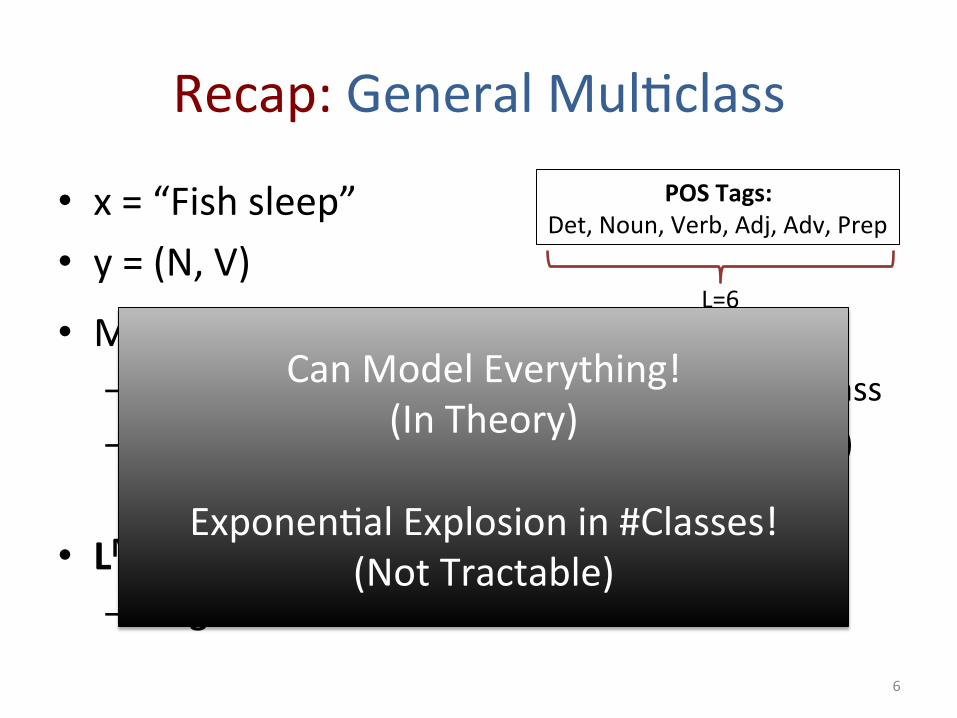
POS Tags: Det, Noun, Verb, Adj, Adv, Prep

L=6

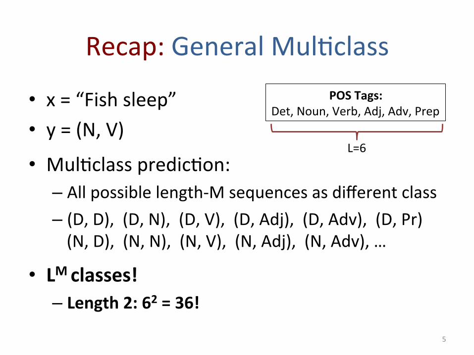
Recap: General Mul5class

•  x = “Fish sleep” •  y = (N, V) •  Mul5class predic5on: – All possible length-‐M sequences as different class –  (D, D), (D, N), (D, V), (D, Adj), (D, Adv), (D, Pr) (N, D), (N, N), (N, V), (N, Adj), (N, Adv), …

•  LM classes! – Length 2: 62 = 36!

5


L=6

Recap: General Mul5class

•  x = “Fish sleep” •  y = (N, V) •  Mul5class predic5on: – All possible length-‐M sequences as different class –  (D, D), (D, N), (D, V), (D, Adj), (D, Adv), (D, Pr) (N, D), (N, N), (N, V), (N, Adj), (N, Adv), …

•  LM classes! – Length 2: 62 = 36!

6


L=6

Can Model Everything! (In Theory)

Exponen5al Explosion in #Classes!

(Not Tractable)

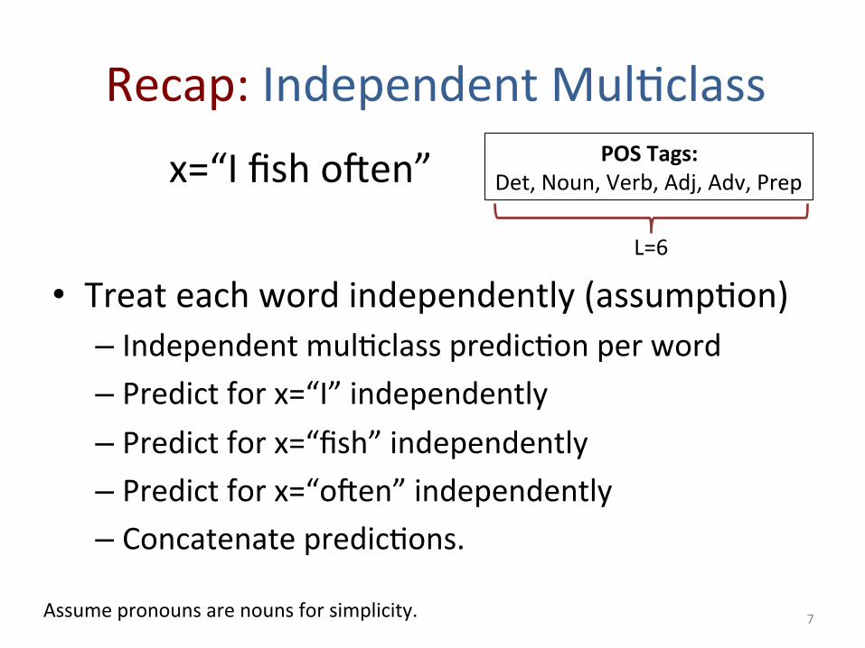
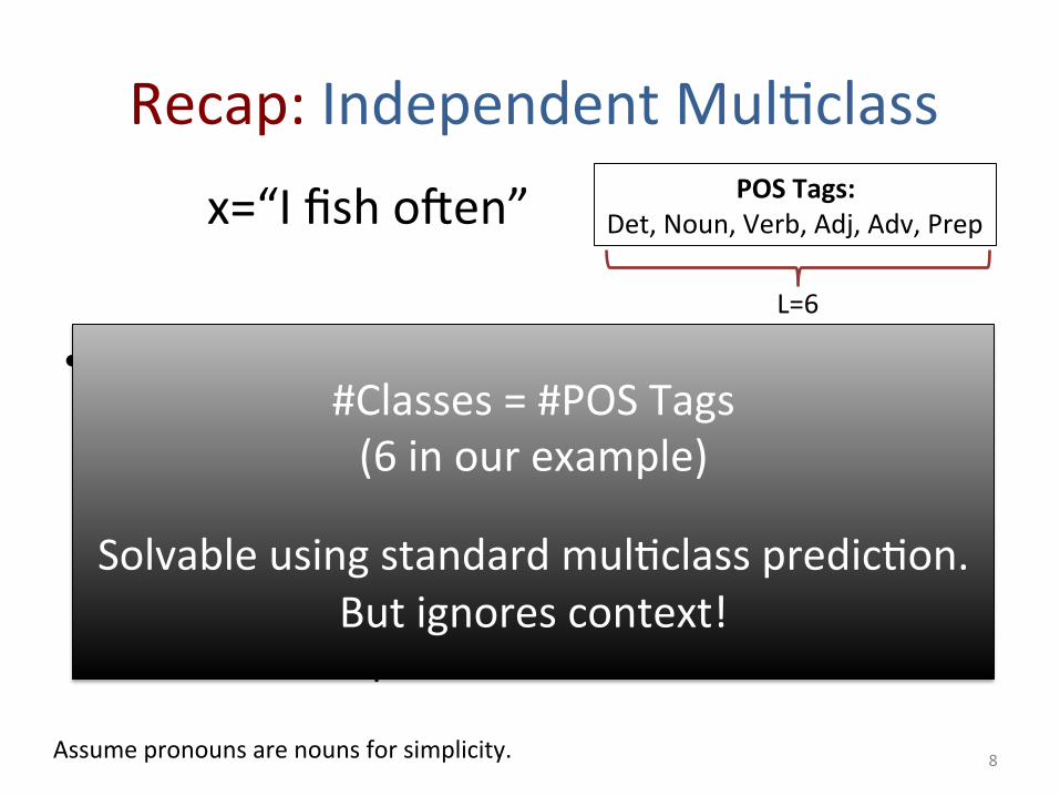
Recap: Independent Mul5class

•  Treat each word independently (assump5on) –  Independent mul5class predic5on per word – Predict for x=“I” independently – Predict for x=“fish” independently – Predict for x=“ojen” independently – Concatenate predic5ons.

7

x=“I fish ojen” POS Tags: Det, Noun, Verb, Adj, Adv, Prep

Assume pronouns are nouns for simplicity.

L=6

Recap: Independent Mul5class

•  Treat each word independently (assump5on) –  Independent mul5class predic5on per word – Predict for x=“I” independently – Predict for x=“fish” independently – Predict for x=“ojen” independently – Concatenate predic5ons.

8

x=“I fish ojen” POS Tags: Det, Noun, Verb, Adj, Adv, Prep

Assume pronouns are nouns for simplicity.

#Classes = #POS Tags (6 in our example)

Solvable using standard mul5class predic5on.

But ignores context!

L=6

Recap: 1st Order HMM

•  x = (x1,x2,x4,x4,…,xM) (sequence of words) •  y = (y1,y2,y3,y4,…,yM) (sequence of POS tags)

•  P(xi|yi) Probability of state yi genera5ng xi •  P(yi+1|yi) Probability of state yi transi5oning to yi+1 •  P(y1|y0) y0 is defined to be the Start state •  P(End|yM) Prior probability of yM being the final state –  Not always used

9

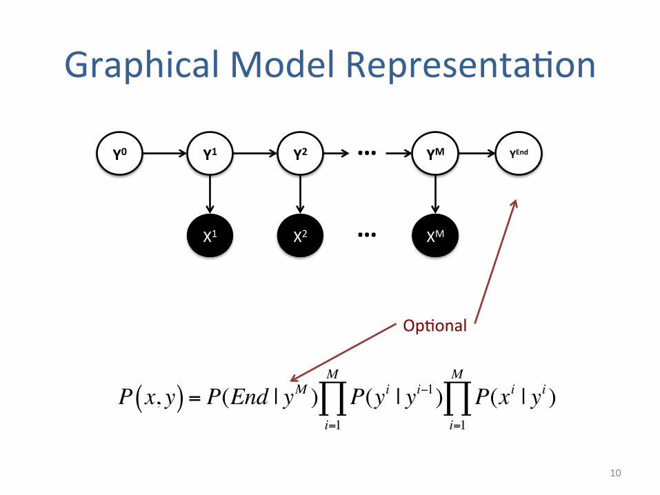
Graphical Model Representa5on

10

Y1

X1

Y2

X2

YM

XM

…

…

P x, y( ) = P(End | yM ) P(yi | yi−1)i=1

M

∏ P(xi | yi )i=1

M

∏

Op5onal

Y0 YEnd

HMM Matrix Formula5on

11

P(x, y) = P(END | yM ) P(x j | y j )j=1

M

∏ P(y j | y j−1)

= AEND,yM

Ay jy j−1

Oyj ,x j

j=1

M

∏

Transi5on Probabili5es Emission Probabili5es (Observa5on Probabili5es)

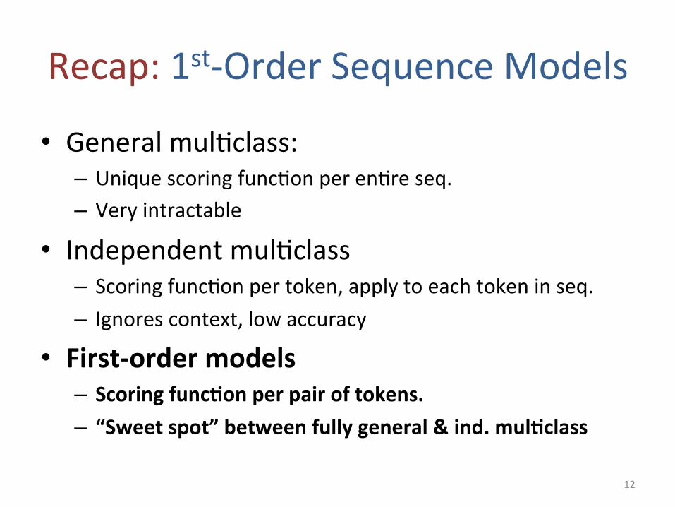
Recap: 1st-‐Order Sequence Models

•  General mul5class: –  Unique scoring func5on per en5re seq. –  Very intractable

•  Independent mul5class –  Scoring func5on per token, apply to each token in seq. –  Ignores context, low accuracy

•  First-‐order models –  Scoring func-on per pair of tokens. –  “Sweet spot” between fully general & ind. mul-class

12

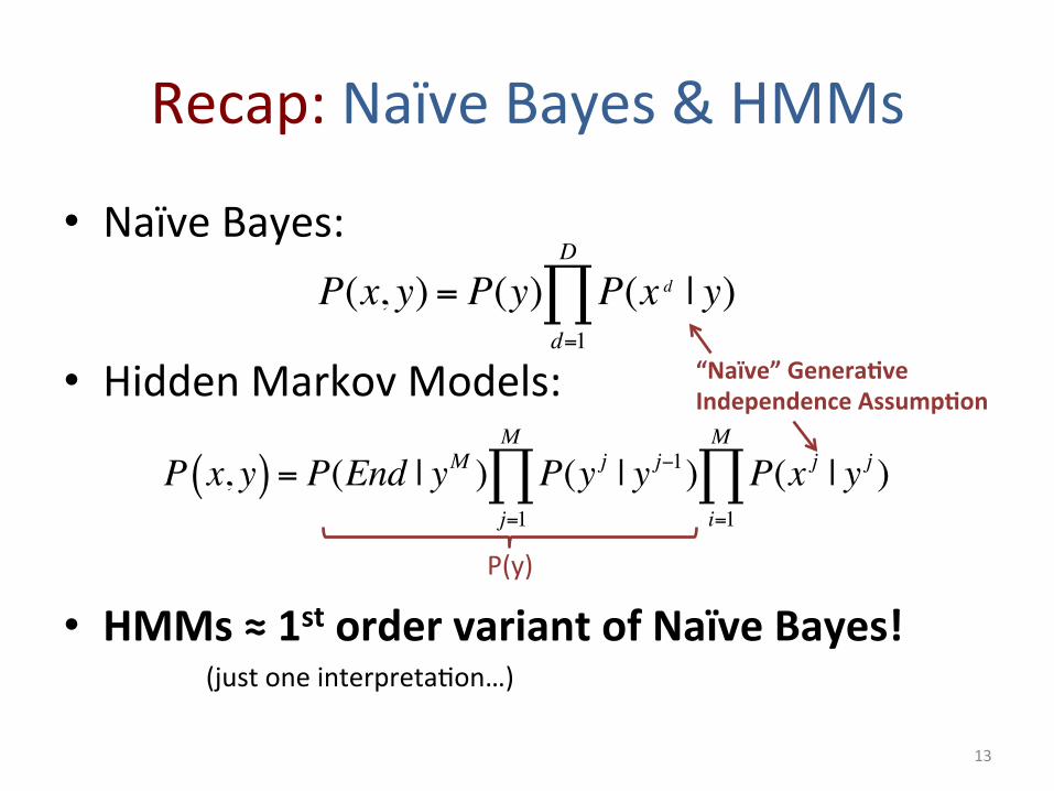
Recap: Naïve Bayes & HMMs

•  Naïve Bayes:

•  Hidden Markov Models:

•  HMMs ≈ 1st order variant of Naïve Bayes!

13

P(x, y) = P(y) P(x d | y)d=1

D

∏

P x, y( ) = P(End | yM ) P(y j | y j−1)j=1

M

∏ P(x j | y j )i=1

M

∏

“Naïve” Genera-ve Independence Assump-on

(just one interpreta5on…)

P(y)

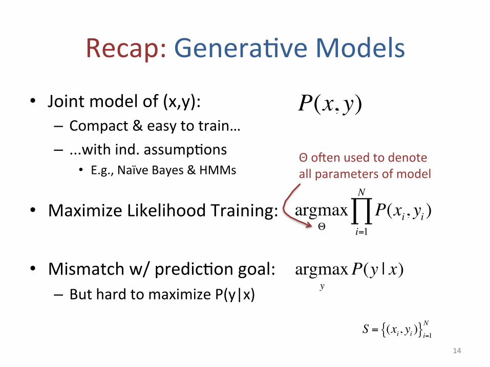
Recap: Genera5ve Models

•  Joint model of (x,y): –  Compact & easy to train… –  ...with ind. assump5ons

•  E.g., Naïve Bayes & HMMs

•  Maximize Likelihood Training:

•  Mismatch w/ predic5on goal: –  But hard to maximize P(y|x)

14

P(x, y)

argmaxΘ

P(xi, yi )i=1

N

∏

Θ ojen used to denote all parameters of model

argmaxy

P(y | x)

S = (xi, yi ){ }i=1N

Learn Condi5onal Prob.?

•  Weird to train to maximize:

•  When goal should be to maximize:

15

argmaxΘ

P(xi, yi )i=1

N

∏

argmaxΘ

P(yi | xi )i=1

N

∏ = argmaxΘ

P(xi, yi )P(xi )i=1

N

∏

p(x) = P(x, y)y∑ = P(y)P(x | y)

y∑Breaks independence!

Can no longer use count sta5s5cs

P(xd = a | y = z) =1

yi=z( )∧ xid=a( )"

#$%i=1

N

∑

1 yi=z[ ]i=1

N

∑ Both HMMs & Naïve Bayes suffer this problem!

S = (xi, yi ){ }i=1N

Learn Condi5onal Prob.?

•  Weird to train to maximize:

•  When goal should be to maximize:

16

argmaxΘ

P(xi, yi )i=1

N

∏

argmaxΘ

P(yi | xi )i=1

N

∏ = argmaxΘ

P(xi, yi )P(xi )i=1

N

∏

p(x) = P(x, y)y∑ = P(y)P(x | y)

y∑Breaks independence!

Can no longer use count sta5s5cs

P(xd = a | y = z) =1

yi=z( )∧ xid=a( )"

#$%i=1

N

∑

1 yi=z[ ]i=1

N

∑ Both HMMs & Naïve Bayes suffer this problem!

S = (xi, yi ){ }i=1N

In general, you should maximize the likelihood of the model you define!

So if you define joint model P(x,y), then maximize P(x,y) on training data.

Genera5ve vs Discrimina5ve

•  Genera5ve Models: –  Joint Distribu5on: P(x,y) –  Uses Bayes’s Rule to predict: argmaxy P(y|x) –  Can generate new samples (x,y)

•  Discrimina5ve Models: –  Condi5onal Distribu5on: P(y|x) –  Can directly to predict: argmaxy P(y|x)

•  Both trained via Maximum Likelihood

17

Same thing!

Hidden Markov Models Naïve Bayes

Condi-onal Random Fields Logis-c Regression

Mismatch!

First Try (for classifying a single y)

•  Model P(y|x) for every possible x

•  Train by coun5ng frequencies •  Exponen-al in # input variables! – Need to assume something… what?

18

P(y=1|x) x1 x2

0.5 0 0

0.7 0 1

0.2 1 0

0.4 1 1

Log Linear Models! (Logis5c Regression)

•  “Log-‐Linear” assump5on – Model representa5on to linear in x – Most common discrimina5ve probabilis5c model

19

argmaxy

P(y | x)

Predic-on:

argmaxΘ

P(yi | xi )i=1

N

∏

Training:

x ∈ RD

y ∈ 1,2,...,L{ }P(y | x) =exp wy

T x − by{ }exp wk

T x − bk{ }k∑

Match!

Naïve Bayes vs Logis5c Regression

•  Naïve Bayes: –  Strong ind. assump5ons –  Super easy to train… –  …but mismatch with predic5on

•  Logis5c Regression: –  “Log Linear” assump5on

•  Ojen more flexible than Naïve Bayes

–  Harder to train (gradient desc.)… –  …but matches predic5on

20

P(x, y) = Ay Oxd ,yd

d=1

D

∏

P(y) P(x|y)

P(y | x) =exp wy

T x − by{ }exp wk

T x − bk{ }k∑

x ∈ RD

y ∈ 1,2,...,L{ }

Naïve Bayes vs Logis5c Regression •  NB has L parameters for P(y) (i.e., A) •  LR has L parameters for bias b

•  NB has L*D parameters for P(x|y) (i.e, O) •  LR has L*D parameters for w

•  Same number of parameters!

21


d=1

D

∏

P(y) P(x|y)

P(y | x) = ewyT x−by

ewkT x−bk

k∑ x ∈ 0,1{ }

D

y ∈ 1,2,...,L{ }

Naïve Bayes Logis5c Regression

Naïve Bayes vs Logis5c Regression •  NB has L parameters for P(y) (i.e., A) •  LR has L parameters for bias b

•  NB has L*D parameters for P(x|y) (i.e, O) •  LR has L*D parameters for w

•  Same number of parameters!

22


d=1

D

∏

P(y) P(x|y)

P(y | x) = ewyT x−by

ewkT x−bk

k∑ x ∈ 0,1{ }

D

y ∈ 1,2,...,K{ }

Naïve Bayes Logis5c Regression

Intui-on: Both models have same “capacity” NB spends a lot of capacity on P(x) LR spends all of capacity on P(y|x)

No Model Is Perfect! (Especially on finite training set) NB will trade off P(y|x) with P(x) LR will fit P(y|x) as well as possible

Condi5onal Random Fields Sequen5al Version of Logis5c Regression

23

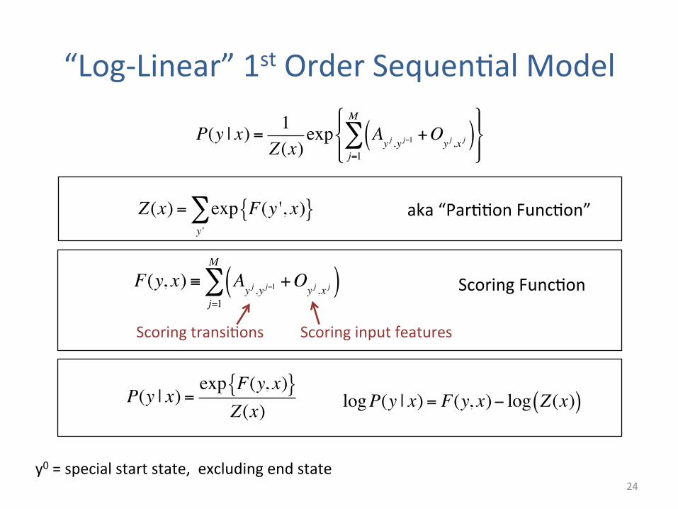
“Log-‐Linear” 1st Order Sequen5al Model

24 y0 = special start state, excluding end state

Scoring transi5ons Scoring input features

P(y | x) =exp F(y, x){ }

Z(x)

F(y, x) ≡ Ayj ,y j−1

+Oyj ,x j( )

j=1

M

∑

logP(y | x) = F(y, x)− log Z(x)( )

Scoring Func5on

Z(x) = exp F(y ', x){ }y '∑ aka “Par55on Func5on”

P(y | x) = 1Z(x)

exp Ayj ,y j−1

+Oyj ,x j( )

j=1

M

∑#$%

&%

'(%

)%

( )

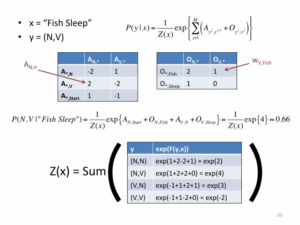
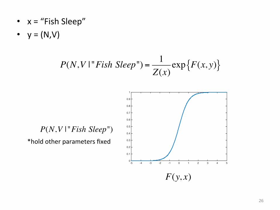
•  x = “Fish Sleep” •  y = (N,V)

25

P(y | x) = 1Z(x)

exp Ayj ,y j−1

+Oyj ,x j( )

j=1

M

∑#$%

&%

'(%

)%

AN,* AV,*

A*,N -‐2 1

A*,V 2 -‐2

A*,Start 1 -‐1

ON,* OV,*

O*,Fish 2 1

O*,Sleep 1 0

AN,V wV,Fish

P(N,V | "Fish Sleep") = 1Z(x)

exp AN ,Start +ON ,Fish + AV ,N +OV ,Sleep{ }= 1Z(x)

exp 4{ } ≈ 0.66

y exp(F(y,x))

(N,N) exp(1+2-‐2+1) = exp(2)

(N,V) exp(1+2+2+0) = exp(4)

(V,N) exp(-‐1+1+2+1) = exp(3)

(V,V) exp(-‐1+1-‐2+0) = exp(-‐2)

Z(x) = Sum

26

-5 -4 -3 -2 -1 0 1 2 3 4 50

0.1

0.2

0.3

0.4

0.5

0.6

0.7

0.8

0.9

1

F(y, x)

•  x = “Fish Sleep” •  y = (N,V)

P(N,V | "Fish Sleep")

P(N,V | "Fish Sleep") = 1Z(x)

exp F(x, y){ }

*hold other parameters fixed

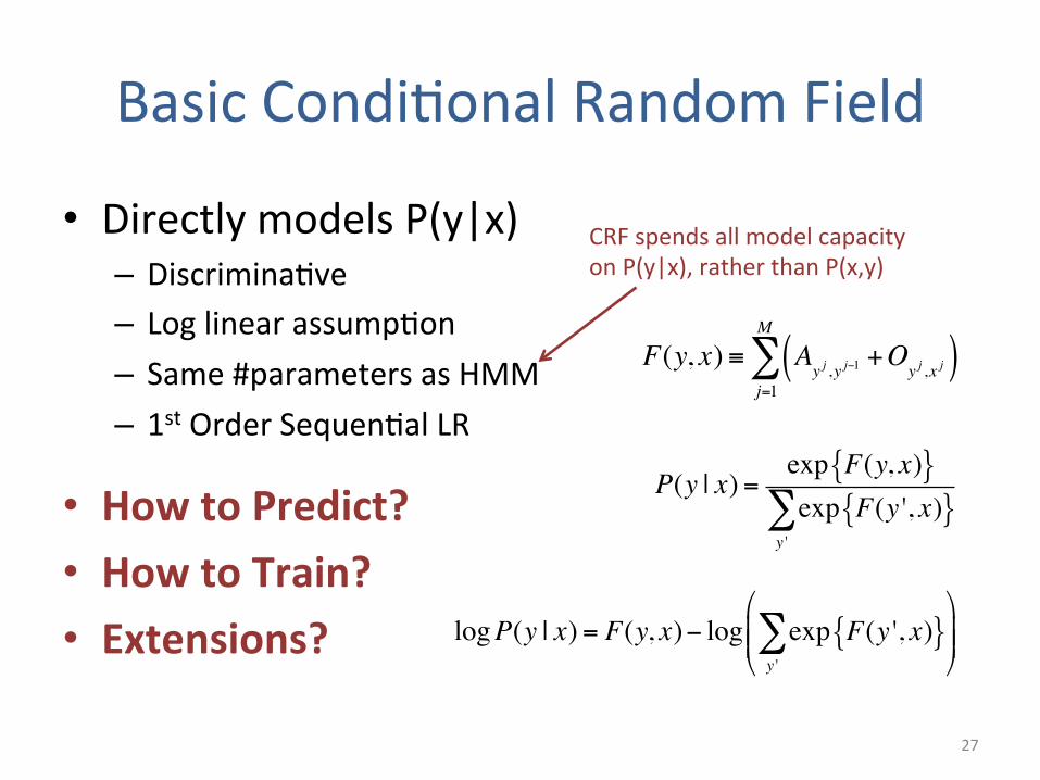
Basic Condi5onal Random Field

•  Directly models P(y|x) –  Discrimina5ve –  Log linear assump5on –  Same #parameters as HMM –  1st Order Sequen5al LR

•  How to Predict? •  How to Train? •  Extensions?

27


+Oyj ,x j( )

j=1

M

∑

P(y | x) =exp F(y, x){ }exp F(y ', x){ }

y '∑

logP(y | x) = F(y, x)− log exp F(y ', x){ }y '∑#

$%%

&

'((

CRF spends all model capacity on P(y|x), rather than P(x,y)

Predict via Viterbi

28

Y k (T ) = argmaxy1:k−1

F(y1:k−1⊕T, x1:k )#

$%

&

'(⊕T

argmaxy

P(y | x) = argmax y

logP(y | x) = argmaxy

F(y, x)

= argmaxy

Aj ,y j−1+O

yj ,x j( )j=1

M

∑

Y k+1(T ) = argmaxy1:k∈ Y k (T ){ }T

F(y1:k ⊕T, x1:k+1)#

$%%

&

'((⊕T

= argmaxy1:k∈ Y k (T ){ }T

F(y1:k, x1:k )+ AT ,yk

+OT ,xk+1

#

$%%

&

'((⊕T

Scoring transi5ons Scoring observa5ons

Maintain length-‐k prefix solu5ons

Recursively solve for length-‐(k+1) solu5ons

argmaxy

F(y, x) = argmaxy∈ Y M (T ){ }T

F(y, x)Predict via best length-‐M solu5on

29

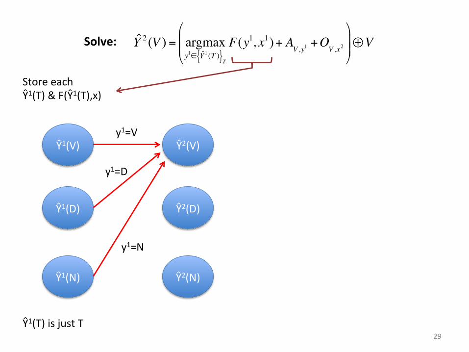
Ŷ1(V)

Ŷ1(D)

Ŷ1(N)

Store each Ŷ1(T) & F(Ŷ1(T),x)

Ŷ2(V)

Ŷ2(D)

Ŷ2(N)

Solve:

y1=V

y1=D

y1=N

Ŷ1(T) is just T

Y 2 (V ) = argmaxy1∈ Y1(T ){ }T

F(y1, x1)+ AV ,y1

+OV ,x2

"

#$$

%

&''⊕V

30

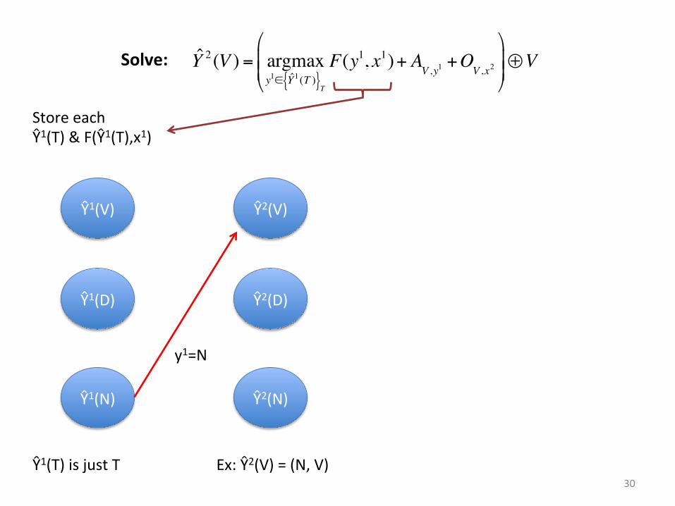
Ŷ1(V)

Ŷ1(D)

Ŷ1(N)

Store each Ŷ1(T) & F(Ŷ1(T),x1)

Ŷ2(V)

Ŷ2(D)

Ŷ2(N)

y1=N

Ŷ1(T) is just T Ex: Ŷ2(V) = (N, V)

Y 2 (V ) = argmaxy1∈ Y1(T ){ }T

F(y1, x1)+ AV ,y1

+OV ,x2

"

#$$

%

&''⊕VSolve:

31

Ŷ1(V)

Ŷ1(D)

Ŷ1(N)

Store each Ŷ1(T) & F(Ŷ1(T),x1)

Ŷ2(V)

Ŷ2(D)

Ŷ2(N)

Store each Ŷ2(Z) & F(Ŷ2(Z),x)

Ex: Ŷ2(V) = (N, V)

Ŷ3(V)

Ŷ3(D)

Ŷ3(N)

Solve:

y2=V

y2=D

y2=N

Y 3(V ) = argmaxy1:2 Y 2 (T ){ }T

F(y1:2, x1:2 )+ AV ,y2

+OV ,x3

!

"##

$

%&&⊕V

Ŷ1(Z) is just Z

32

Ŷ1(V)

Ŷ1(D)

Ŷ1(N)

Store each Ŷ1(Z) & F(Ŷ1(Z),x1)

Ŷ2(V)

Ŷ2(D)

Ŷ2(N)


Ex: Ŷ2(V) = (N, V)

Ŷ3(V)

Ŷ3(D)

Ŷ3(N)


Ex: Ŷ3(V) = (D,N,V)

ŶL(V)

ŶL(D)

ŶL(N)

…

Ŷ1(T) is just T

Y M (V ) = argmaxyM−1∈ Y M (T ){ }T

F(y1:M−1, x1:M−1)+ AV ,yM−1 +OV ,xM

#

$%%

&

'((⊕VSolve:

Compu5ng P(y|x)

•  Viterbi doesn’t compute P(y|x) –  Just maximizes the numerator F(y,x)

•  Also need to compute Z(x) – aka the “Par55on Func5on”

33

P(y | x) =exp F(y, x){ }exp F(y ', x){ }

y '∑

≡1

Z(x)exp F(y, x){ }

Z(x) = exp F(y ', x){ }y '∑

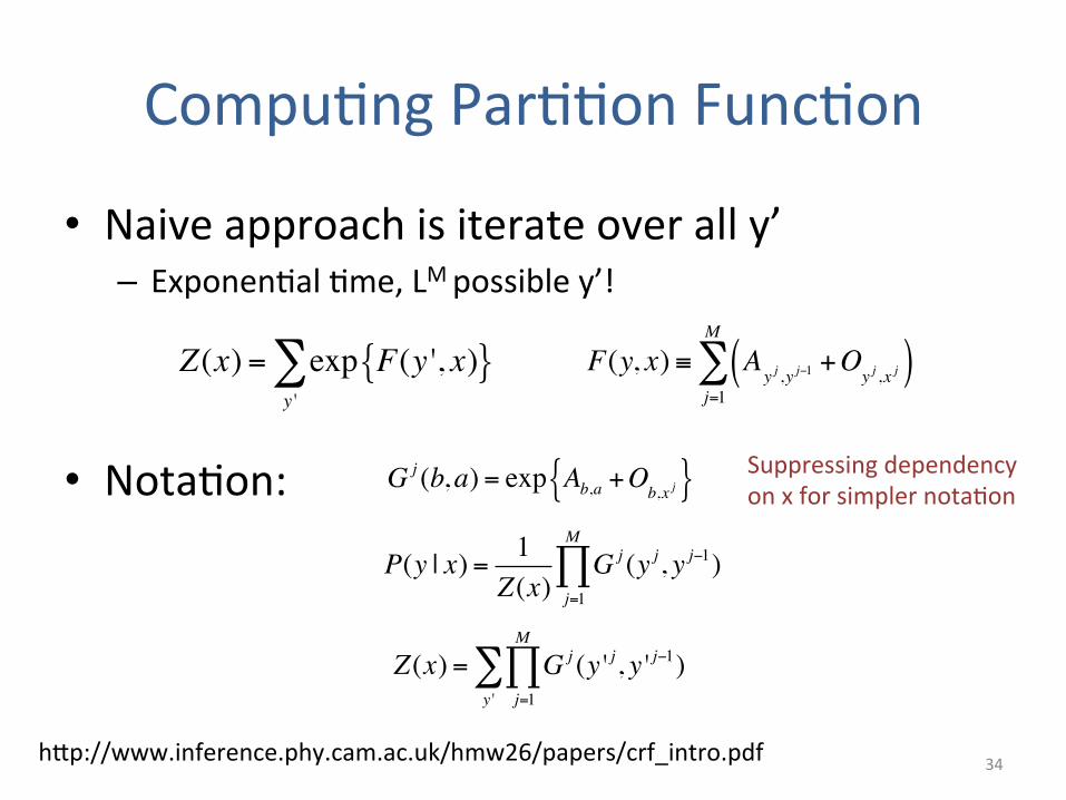
Compu5ng Par55on Func5on

•  Naive approach is iterate over all y’ –  Exponen5al 5me, LM possible y’!

•  Nota5on:

34

Z(x) = exp F(y ', x){ }y '∑

G j (b,a) = exp Ab,a +Ob,x j{ }


+Oyj ,x j( )

j=1

M

∑

P(y | x) = 1Z(x)

G j (y j, y j−1)j=1

M

∏

Z(x) = G j (y ' j, y ' j−1)j=1

M

∏y '∑

hyp://www.inference.phy.cam.ac.uk/hmw26/papers/crf_intro.pdf

Suppressing dependency on x for simpler nota5on

Matrix Semiring

35

G j (b,a) = exp Ab,a +Oa,x j{ }

Z(x) = G j (y ' j, y ' j−1)j=1

M

∏y '∑ = G1:M (b,a)

b,a∑

Gj(a,b)

L+1

Matrix Version of Gj

G1:2 (b,a) ≡ G2 (b,c)G1(c,a)c∑ G1:2 G2 G1 =

Gi:j Gi+1 Gi = Gj Gj-‐1 … Gi: j (b,a) ≡

L+1

Include ‘Start’


Path Coun5ng Interpreta5on

•  Interpreta5on G1(b,a) – L+1 start & end loca5ons – Weight of path from ‘a’ to ‘b’ in step 1

•  G1:2(b,a) – Weight of all paths

•  Start in ‘a’ beginning of Step 1 •  End in ‘b’ ajer Step 2

36

G1

G1:2 G2 G1 =


•  Consider Length-‐1 (M=1)

•  M=2

•  General M –  Do M (L+1)x(L+1) matrix computa5ons to compute G1:M

–  Z(x) = sum column ‘Start’ of G1:M


37

Z(x) = G1(b,Start)b∑

Sum column ‘Start’ of G1!

Z(x) = G2 (b,a)G1(a,Start)a,b∑ = G1:2 (b,Start)

b∑

Sum column ‘Start’ of G1:2!

G1:M G2 G1 = GM GM-‐1 …

Sum column ‘Start’ of G1:M!


•  Consider Length-‐1 (M=1)

•  M=2

•  General M –  Do M (L+1)x(L+1) matrix computa5ons to compute G1:M

–  Z(x) = sum column ‘Start’ of G1:M


38

Z(x) = G1(b,Start)b∑

Sum column ‘Start’ of G1!

Z(x) = G2 (b,a)G1(a,Start)a,b∑ = G1:2 (b,Start)

b∑

Sum column ‘Start’ of G1:2!

G1:M G2 G1 = GM GM-‐1 …

Sum column ‘Start’ of G1:M!


Numerical Instability Issues! (See Course Notes)

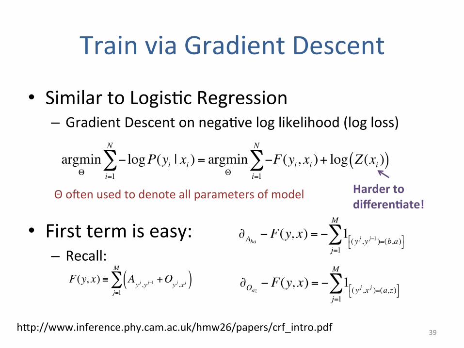
Train via Gradient Descent

•  Similar to Logis5c Regression –  Gradient Descent on nega5ve log likelihood (log loss)

•  First term is easy: –  Recall:

39

argminΘ

− logP(yi | xi )i=1

N

∑ = argminΘ

−F(yi, xi )+ log Z(xi )( )i=1

N

∑

Θ ojen used to denote all parameters of model

∂Aba −F(y, x) = − 1(y j ,y j−1 )=(b,a)#$

%&

j=1

M

∑


+Oyj ,x j( )

j=1

M

∑ ∂Oaz −F(y, x) = − 1(y j ,x j )=(a,z)#$

%&

j=1

M

∑

Harder to differen-ate!


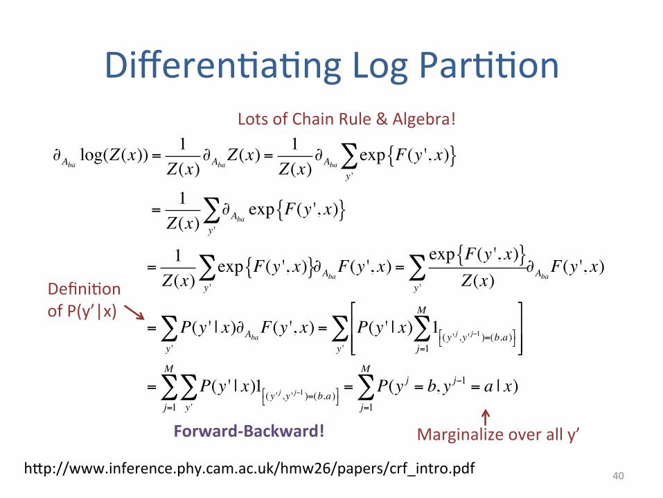
Differen5a5ng Log Par55on

40

∂Aba log(Z(x)) = 1Z(x)

∂AbaZ(x) = 1Z(x)

∂Aba exp F(y ', x){ }y '∑

= 1Z(x)

∂Aba exp F(y ', x){ }y '∑

= 1Z(x)

exp F(y ', x){ }y '∑ ∂AbaF(y ', x) =

exp F(y ', x){ }Z(x)y '

∑ ∂AbaF(y ', x)

= P(y ' | x)∂AbaF(y ', x)y '∑ = P(y ' | x) 1

(y ' j ,y ' j−1 )=(b,a)$%

&'

j=1

M

∑$

%((

&

'))y '

∑

= P(y ' | x)1(y ' j ,y ' j−1 )=(b,a)$%

&'

y '∑

j=1

M

∑ = P(y j = b, y j−1 = a | x)j=1

M

∑

Lots of Chain Rule & Algebra!

Defini5on of P(y’|x)

Marginalize over all y’


Forward-‐Backward!

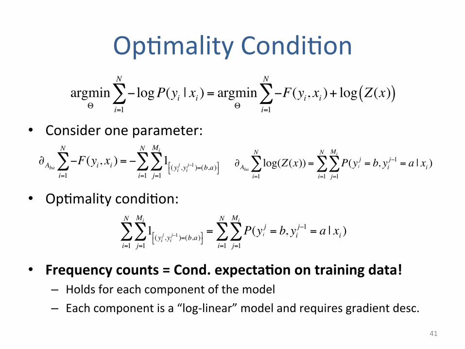
Op5mality Condi5on

•  Consider one parameter:

•  Op5mality condi5on:

•  Frequency counts = Cond. expecta-on on training data! –  Holds for each component of the model –  Each component is a “log-‐linear” model and requires gradient desc.

41

∂Aba log(Z(x))i=1

N

∑ = P(yij = b, yi

j−1 = a | xi )j=1

Mi

∑i=1

N

∑∂Aba −F(yi, xi )i=1

N

∑ = − 1(yi

j ,yij−1 )=(b,a)$

%&'

j=1

Mi

∑i=1

N

∑

argminΘ

− logP(yi | xi )i=1

N

∑ = argminΘ

−F(yi, xi )+ log Z(x)( )i=1

N

∑

1(yi

j ,yij−1 )=(b,a)"

#$%

j=1

Mi

∑i=1

N

∑ = P(yij = b, yi

j−1 = a | xi )j=1

Mi

∑i=1

N

∑

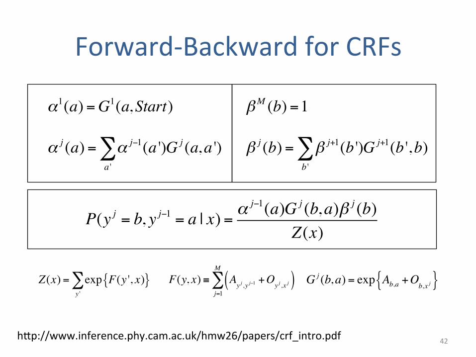
Forward-‐Backward for CRFs

42 hyp://www.inference.phy.cam.ac.uk/hmw26/papers/crf_intro.pdf

P(y j = b, y j−1 = a | x) = αj−1(a)G j (b,a)β j (b)

Z(x)

α1(a) =G1(a,Start)

α j (a) = α j−1(a ')G j (a,a ')a '∑

βM (b) =1

β j (b) = β j+1(b ')G j+1(b ',b)b '∑

G j (b,a) = exp Ab,a +Ob,x j{ }Z(x) = exp F(y ', x){ }y '∑ F(y, x) ≡ A

yj ,y j−1+O

yj ,x j( )j=1

M

∑

Path Interpreta5on

43

α1(V)

α1(D)

α1(N)

α2(V)

α2(D)

α2(N)

α3(V)

α3(D)

α3(N)

α1 α2 α3

“Start”

G1(V,“Start”)

G1(N,“Start”)

x G2(D,N) x G3(N,D)

Total Weight of paths from “Start” to “V” in 3rd step

β just does it backwards

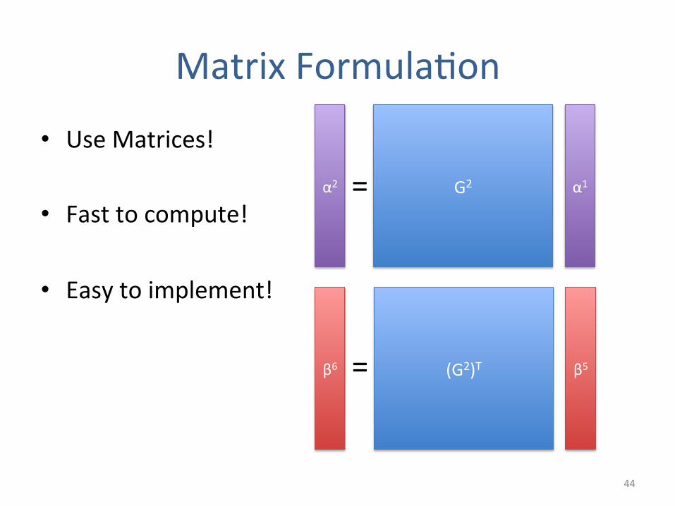
Matrix Formula5on

44

G2 α1 α2 =

(G2)T β5 β6 =

•  Use Matrices!

•  Fast to compute!

•  Easy to implement!

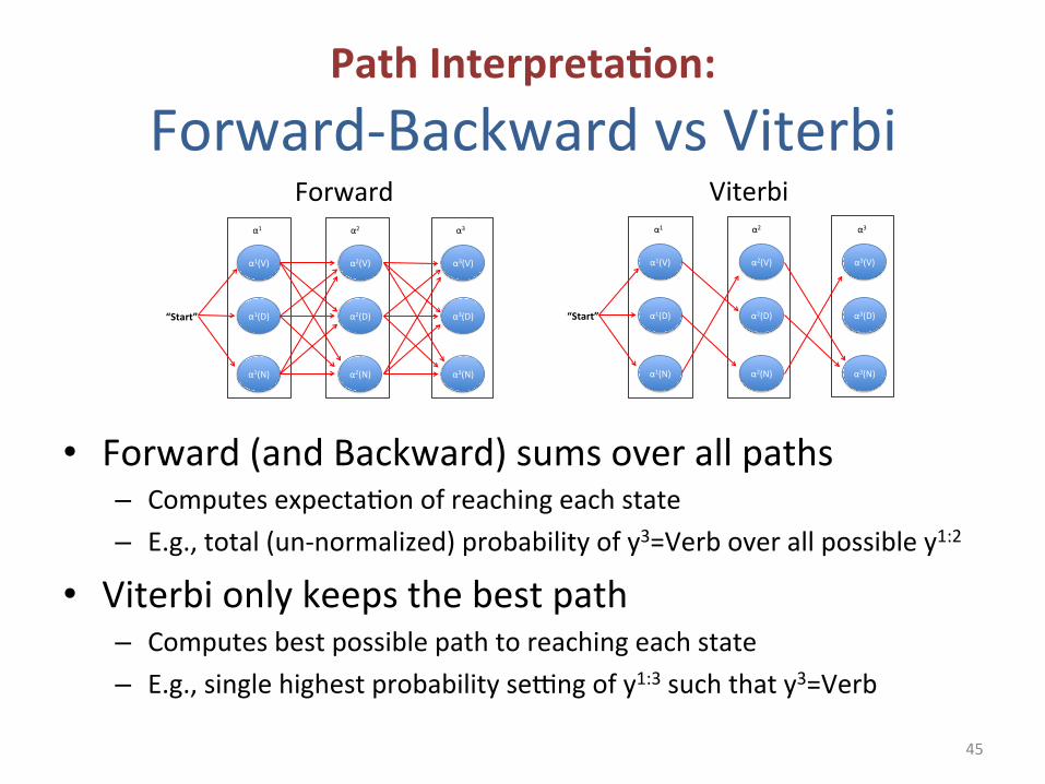
Path Interpreta-on: Forward-‐Backward vs Viterbi

•  Forward (and Backward) sums over all paths –  Computes expecta5on of reaching each state –  E.g., total (un-‐normalized) probability of y3=Verb over all possible y1:2

•  Viterbi only keeps the best path –  Computes best possible path to reaching each state –  E.g., single highest probability se~ng of y1:3 such that y3=Verb

45

Path%Interpreta+on%

38%

α1(V)%

α1(D)%

α1(N)%

α2(V)%

α2(D)%

α2(N)%

α3(V)%

α3(D)%

α3(N)%

α1% α2% α3%

“Start”'

β%just%does%it%backwards%%

Path%Interpreta+on%

38%

α1(V)%

α1(D)%

α1(N)%

α2(V)%

α2(D)%

α2(N)%

α3(V)%

α3(D)%

α3(N)%

α1% α2% α3%

“Start”'

β%just%does%it%backwards%%

Forward Viterbi

Summary: Training CRFs

•  Similar op5mality condi5on as HMMs: – Match frequency counts of model components!

– Except HMMs can just set the model using counts – CRFs need to do gradient descent to match counts

•  Run Forward-‐Backward for expecta5on –  Just like HMMs as well

46

1(yi

j ,yij−1 )=(b,a)"

#$%

j=1

Mi

∑i=1

N

∑ = P(yij = b, yi

j−1 = a | xi )j=1

Mi

∑i=1

N

∑

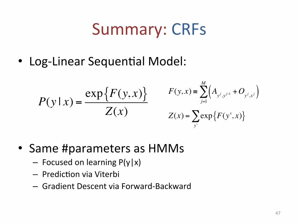
Summary: CRFs

•  Log-‐Linear Sequen5al Model:

•  Same #parameters as HMMs –  Focused on learning P(y|x) –  Predic5on via Viterbi –  Gradient Descent via Forward-‐Backward

47

P(y | x) =exp F(y, x){ }

Z(x)


+Oyj ,x j( )

j=1

M

∑

Z(x) = exp F(y ', x){ }y '∑

Next Lecture

•  More General Formula5on of CRFs – More concise nota5on

•  Matches logis5c regression nota5on •  Matches course notes (later this week)

– Easier to reason about for implementa5on

•  General Structured Predic5on

48

Machine(Learning(&(DataMining - Yisong · PDF fileToday(•...

Documents

Transcript of Machine(Learning(&(DataMining - Yisong · PDF fileToday(•...