Machine semantics
23
Theoretical Computer Science 409 (2008) 1–23 Contents lists available at ScienceDirect Theoretical Computer Science journal homepage: www.elsevier.com/locate/tcs Machine semantics ✩ Peter Hines * Department of Computer Science, York University, York, UK article info Article history: Received 8 June 2006 Received in revised form 4 July 2008 Accepted 19 July 2008 Communicated by P.-L. Curien Keywords: Geometry of interaction Domain theory Category theory Bounded turing machines Enriched semigroups Physical computing abstract Using simple systems with a notion of discrete deterministic evolution over time, we study discrete causality via tools from theoretical computer science and logic. We consider the set of all representations (i.e. partial descriptions) of such systems, from algebraic, domain- theoretic, and categorical viewpoints. The order theory introduced, is based in the notion of comparing high-level and low- level descriptions of the same system. This is shown to give a Complete Partial Order where the down-closure of each element is a locale. This partial order has a very close connection to a categorical construction known as the ‘particle-style’ trace, via analogues of domain-theoretic equations. Thus, the trace may be thought of as the computation of suprema in this partial order. As a sample application, we show how to construct algebraic models of space-bounded Turing machines in these terms, and derive compositionality from the abstract properties of the trace. © 2008 Elsevier B.V. All rights reserved. 1. Introduction This paper is a study of a simple notion of discrete causality, using tools from domain theory, category theory, and other areas of theoretical computer science. We axiomatise causality in terms of structures that we call Abstract Machines. These simply consist of a set of configurations, and a partial deterministic rule called the primitive evolution that, given a current configuration, specifies the unique next configuration (provided it exists). Although such a definition has been given many times under many names in theoretical computer science and other subjects, 1 we emphasise that Abstract Machines themselves need not be explicitly computational devices — rather, we are using them as a simple notion of causality, in order to use tools from theoretical computer science to study causality itself. The programme of using tools from theoretical computer science to study this form of causality was started in [25], where a very restricted case was considered — this paper considers the general case. For an Abstract Machine, we consider the set of all partial functions that provide a (generally incomplete, or partial) description of its behaviour. We refer to this set (in fact, semigroup) as the machine semantics. We then consider the structure of this semigroup, including how these competing representations of the Abstract Machine may be compared with each other — we use order-theoretic methods to contrast ‘high-level’ and ‘low-level’ descriptions of its behaviour. This gives a rich order theory, based on Complete Partial Orders and locales. We then consider connections between this order theory, and the particle-style, or iterative categorical trace. The particle- style trace is shown to satisfy properties very similar to an order-theoretic supremum, and is exactly the computation of the supremum of a naturally defined sub-lattice when restricted to the order-theoretic case. ✩ Expanded version of the talk ‘Random thoughts on Abstract Machines’ presented at the Bellairs Research Center (Barbados, March 2006). * Tel.: +44 904 433378. E-mail address: [email protected]. 1 For example, we refer to [39] for unlabelled transition systems, and the apposite comment that, ‘Of course, such an idea is hardly new, and examples can be found in any book on automata or formal languages’. 0304-3975/$ – see front matter © 2008 Elsevier B.V. All rights reserved. doi:10.1016/j.tcs.2008.07.015
-
Upload
peter-hines -
Category
Documents
-
view
220 -
download
0
Transcript of Machine semantics

Theoretical Computer Science 409 (2008) 1–23
Contents lists available at ScienceDirect
Theoretical Computer Science
journal homepage: www.elsevier.com/locate/tcs
Machine semanticsI
Peter Hines ∗Department of Computer Science, York University, York, UK
a r t i c l e i n f o
Article history:Received 8 June 2006Received in revised form 4 July 2008Accepted 19 July 2008Communicated by P.-L. Curien
Keywords:Geometry of interactionDomain theoryCategory theoryBounded turing machinesEnriched semigroupsPhysical computing
a b s t r a c t
Using simple systemswith a notion of discrete deterministic evolution over time, we studydiscrete causality via tools from theoretical computer science and logic. We consider theset of all representations (i.e. partial descriptions) of such systems, from algebraic, domain-theoretic, and categorical viewpoints.The order theory introduced, is based in the notion of comparing high-level and low-
level descriptions of the same system. This is shown to give a Complete Partial Orderwherethe down-closure of each element is a locale.This partial order has a very close connection to a categorical construction known as
the ‘particle-style’ trace, via analogues of domain-theoretic equations. Thus, the trace maybe thought of as the computation of suprema in this partial order. As a sample application,we show how to construct algebraic models of space-bounded Turing machines in theseterms, and derive compositionality from the abstract properties of the trace.
© 2008 Elsevier B.V. All rights reserved.
1. Introduction
This paper is a study of a simple notion of discrete causality, using tools from domain theory, category theory, and otherareas of theoretical computer science. We axiomatise causality in terms of structures that we call Abstract Machines. Thesesimply consist of a set of configurations, and a partial deterministic rule called the primitive evolution that, given a currentconfiguration, specifies the unique next configuration (provided it exists).Although such a definition has been given many times under many names in theoretical computer science and other
subjects,1 we emphasise that Abstract Machines themselves need not be explicitly computational devices — rather, we areusing them as a simple notion of causality, in order to use tools from theoretical computer science to study causality itself.The programme of using tools from theoretical computer science to study this formof causalitywas started in [25], where
a very restricted case was considered — this paper considers the general case. For an Abstract Machine, we consider the setof all partial functions that provide a (generally incomplete, or partial) description of its behaviour. We refer to this set (infact, semigroup) as themachine semantics. We then consider the structure of this semigroup, including how these competingrepresentations of the Abstract Machine may be compared with each other — we use order-theoretic methods to contrast‘high-level’ and ‘low-level’ descriptions of its behaviour. This gives a rich order theory, based on Complete Partial Ordersand locales.We then consider connections between this order theory, and the particle-style, or iterative categorical trace. The particle-
style trace is shown to satisfy properties very similar to an order-theoretic supremum, and is exactly the computation of thesupremum of a naturally defined sub-lattice when restricted to the order-theoretic case.
I Expanded version of the talk ‘Random thoughts on Abstract Machines’ presented at the Bellairs Research Center (Barbados, March 2006).∗ Tel.: +44 904 433378.E-mail address: [email protected] For example, we refer to [39] for unlabelled transition systems, and the apposite comment that, ‘Of course, such an idea is hardly new, and examples can
be found in any book on automata or formal languages’.
0304-3975/$ – see front matter© 2008 Elsevier B.V. All rights reserved.doi:10.1016/j.tcs.2008.07.015

2 P. Hines / Theoretical Computer Science 409 (2008) 1–23
Fig. 1. An Abstract Machine as a directed graph.
As an example application, we study algebraic models of space-bounded Turing machines in these terms. Althoughalgebraic models have previously been derived by a brute-force analysis [24], the framework of CPOs and the particle-styletrace, demonstrates why both the particle-style trace, and the corresponding Geometry of Interaction construction, appearin this seemingly unrelated context. The abstract properties of the trace also give compositionality of these algebraicmodelsfor free, using the same categorical structures commonly used to model confluence in logical systems.
2. Definitions
The basic definitions below are taken from [25]. However, the terminology and notation used has changed somewhat,for clarity.Definition 1 (Abstract Machines, Configurations, the Primitive Evolution). An Abstract Machine, or A.M., consists of a set Xof configurations, together with a partial function P : X → X called the primitive evolution. We will often treat P as a(special type of) relation — in particular, the transitive closure of P plays a vital rôle in this paper.Abstract Machines may be drawn as directed graphs, as shown in Fig. 1, although not all directed graphs specify an AbstractMachine. We use such diagrams throughout, to illustrate key concepts.As the definition of an Abstract Machine is very broad, a wide range of computational examples are available:
Examples.(1) (Deterministic) Turing machines — a configuration is a specification of the tape contents, together with the position andlabel of the machine head. The primitive evolution is given by the transition rule for the T.M.
(2) Assorted variants on deterministic state machines (finite state/two-way/Mealy automata, space/time bounded T.M.s,&c.). These can be given (as in [24]) as special cases of (1).
(3) Cellular automata — a configuration is a specification of the contents of every cell, and the primitive evolution is givenby the neighbourhood rule.
(4) Universal register machines — a configuration is the contents of all registers, and the primitive evolution is immediate.(5) von Neumann computers — a configuration is a specification of the memory contents, and the primitive evolution isgiven by the fetch-execute cycle. We will use this as the canonical example of an Abstract Machine, in order to motivatevarious general definitions.
(6) A quantum computer executing Grover’s algorithm. A configuration is a specification of the contents of the quantumregisters, and the primitive evolution is the ‘inversion about the mean’ unitary map.2
(7) The linear combinators of [4]. This follows from the intuition of the trace on partial functions (see Section 7) as ‘a particlemoving through a labelled network’ [1], and an exact specification of the configurations and primitive evolution is aninteresting, non-trivial exercise.
Although the above are all computational examples, any system that evolves in deterministic discrete steps may beconsidered as an Abstract Machine. Sometimes, as in (5) and (6) above, the distinction between computational and physicalexamples is somewhat blurred & some authors (notably [46]) claim that such a distinction is entirely arbitrary.An interesting non-example is that of the pure untyped lambda calculus. It is tempting to think of lambda-terms as
configurations, and β-reduction as the primitive evolution. However, arbitrary λ-terms can be reduced in many differentways, so we do not have a deterministic partial function to act as the primitive evolution. Given a fixed deterministicreduction strategy, λ-calculus may be treated as an Abstract Machine, but this clearly misses much of the interestingstructure of β-reduction.
2.1. Tools to study Abstract Machines
The above definition of a set, together with a partial function acting on it, is of course not original. This paper differs inthe questions we ask, and hence the tools used, in the study of these structures. We now make a few basic definitions:
2 There are, as may be expected, various subtleties in this example. It is considered further in Section 10.

P. Hines / Theoretical Computer Science 409 (2008) 1–23 3
Definition 2 (The ;Relation, Representations, Machine Semantics). LetM = (X,P ) be an Abstract Machine. The relation
;on X is defined to be the transitive closure of the primitive evolution, so ;=⋃∞
n=1 P n. This is the smallest binaryrelation satisfying:
• P (x) = y implies that y ;x• c ;b and b ;a implies that c ;a.
We read v ;u as, ‘u leads to v.A representation ofM is a partial function η : X → X satisfying y = η(x) implies y ;x (i.e. the diagonal representation
of η is a subset of ;). Representations are far from unique — we observe that both the primitive evolutionP : X → X andthe nowhere-defined partial function 0X : X → X are representations ofM. The set of all representations ofM is called themachine semantics forM, denoted [M].The machine semantics is a subset of the set of all partial functions from X to itself. We demonstrate that it is also
closed under the usual composition and summation of partial functions (and hence is a semigroup enriched over an additivestructure).
Definition 3 (Composition and Summation of Partial Functions). Given partial functions f : X → Y and g : Y → Z , theircomposite gf : X → Z is defined by
gf (x) ={g(f (x)) x ∈ dom(f ) and f (x) ∈ dom(g)undefined otherwise.
An indexed family of partial functions {fi : X → Y }i∈I is summable exactly when dom(fi) ∩ dom(fj) = ∅ for all i 6= j. Thesum is given by(∑
i∈I
fi
)(x) =
{fi(x) x ∈ dom(fi)undefined otherwise.
It is a standard result that composition distributes over summation, so given a summable family {fi}i∈I and arbitraryg : U → X , h : Y → Z ,
h
(∑i∈I
fi
)g =
∑i∈I
hfig.
We refer to [35] for detailed study of this summation, including a proof of distributivity, and applications in programsemantics of conditional iteration, and [27] for a demonstration that this summation arises from a genuine categoricalenrichment.
Lemma 4. LetM = (X,P ) be an A.M. Then(1) [M] is closed under composition of partial functions, and hence is a semigroup with a zero.(2) [M] is closed under the partial summation of Definition 3.
Proof. (1) (The fact that [M] is a semigroup is stated but not proved in [25]). Consider representations η, µ. If ηµ = 0X ,then we are done, since 0X is by definition a representation. Whenµη 6= 0X , there exists some x ∈ X with η(x) = y andµ(y) = z = µη(x). However, representations are characterised by the condition η(x) = y ⇒ y ;x. By definition, ;
is transitive, and so z ;x. Hence µη is also a representation ofM. Finally, the nowhere-defined partial function 0X istrivially a representation ofM, and hence is a zero for this semigroup.
(2) Consider a summable indexed family of representations, {ηi}i∈I ⊆ [M]. From Definition 3, their sum is given by(∑i∈I
ηi
)(x) =
{ηi(x) x ∈ dom(ηi)undefined otherwise.
It is immediate that(∑
i∈I ηi)(x) ;x, and so this is also a representation. �
2.2. Representations of a von Neumann machine
For motivation, we now provide an example of distinct representations in a familiar setting. Using a von Neumannmachine, as the canonical example of an Abstract Machine, consider the following situation:
The von Neumannmachine is a desktop P.C., running a JAVA program, that is compiled into Interpreted Byte Code, andexecuted on a chip based on the von Neumann architecture.
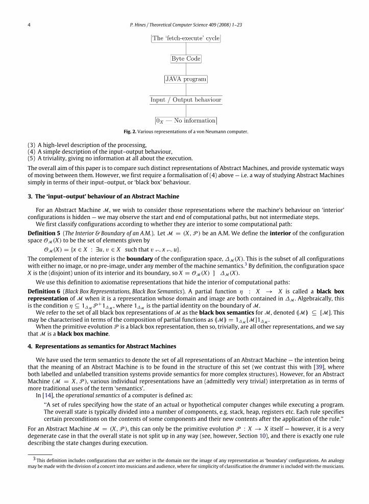
Various representations of this are shown in Fig. 2. These all describe, at different levels of generality, the same machine.We have(1) A complete step-by-step description of the execution,(2) A low-level description of the processing,
4 P. Hines / Theoretical Computer Science 409 (2008) 1–23
Fig. 2. Various representations of a von Neumann computer.
(3) A high-level description of the processing,(4) A simple description of the input–output behaviour,(5) A triviality, giving no information at all about the execution.
The overall aim of this paper is to compare such distinct representations of Abstract Machines, and provide systematic waysof moving between them. However, we first require a formalisation of (4) above — i.e. a way of studying Abstract Machinessimply in terms of their input–output, or ‘black box’ behaviour.
3. The ‘input–output’ behaviour of an Abstract Machine
For an Abstract Machine M, we wish to consider those representations where the machine’s behaviour on ‘interior’configurations is hidden — we may observe the start and end of computational paths, but not intermediate steps.We first classify configurations according to whether they are interior to some computational path:
Definition 5 (The Interior & Boundary of an A.M.). LetM = (X,P ) be an A.M. We define the interior of the configurationspace OM(X) to be the set of elements given by
OM(X) = {x ∈ X : ∃u, v ∈ X such that v ;x ;u}.The complement of the interior is the boundary of the configuration space, ∆M(X). This is the subset of all configurationswith either no image, or no pre-image, under anymember of themachine semantics.3 By definition, the configuration spaceX is the (disjoint) union of its interior and its boundary, so X = OM(X) ] ∆M(X).We use this definition to axiomatise representations that hide the interior of computational paths:
Definition 6 (Black Box Representations, Black Box Semantics). A partial function η : X → X is called a black boxrepresentation ofM when it is a representation whose domain and image are both contained in ∆M . Algebraically, thisis the condition η ⊆ 1∆MP+1∆M , where 1∆M is the partial identity on the boundary ofM.We refer to the set of all black box representations ofM as the black box semantics forM, denoted (|M|) ⊆ [M]. This
may be characterised in terms of the composition of partial functions as (|M|) = 1∆M [M]1∆M .When the primitive evolutionP is a black box representation, then so, trivially, are all other representations, and we say
thatM is a black box machine.
4. Representations as semantics for Abstract Machines
We have used the term semantics to denote the set of all representations of an Abstract Machine — the intention beingthat the meaning of an Abstract Machine is to be found in the structure of this set (we contrast this with [39], whereboth labelled and unlabelled transition systems provide semantics for more complex structures). However, for an AbstractMachine (M = X,P ), various individual representations have an (admittedly very trivial) interpretation as in terms ofmore traditional uses of the term ‘semantics’.In [14], the operational semantics of a computer is defined as:‘‘A set of rules specifying how the state of an actual or hypothetical computer changes while executing a program.The overall state is typically divided into a number of components, e.g. stack, heap, registers etc. Each rule specifiescertain preconditions on the contents of some components and their new contents after the application of the rule.’’
For an Abstract MachineM = (X,P ), this can only be the primitive evolution P : X → X itself — however, it is a verydegenerate case in that the overall state is not split up in any way (see, however, Section 10), and there is exactly one ruledescribing the state changes during execution.
3 This definition includes configurations that are neither in the domain nor the image of any representation as ‘boundary’ configurations. An analogymay bemadewith the division of a concert intomusicians and audience, where for simplicity of classification the drummer is includedwith themusicians.

P. Hines / Theoretical Computer Science 409 (2008) 1–23 5
Fig. 3. The primitiveness relation.
By distinction, [35] informally introduces the denotational semantics of a computer as,
‘‘By contrast to the operational semantics which traces all intermediate states in a computer program, denotationalsemantics focuses on the input/output behaviour and ignores the intermediate states.’’
Again, this is almost trivial: any black box representation satisfies this informal specification. We will later show that theset of all black box representations forms a lattice, so we take the top element of this lattice as the denotational semantics.However, this is again a remarkably degenerate case — by contrast, we compare this with the use of fixed-point propertiesin domain theory, to provide denotational semantics of recursively defined programs as given in (for example) [43].If these two extremes were the only objects of study, there would be very little to say about semantics of Abstract
Machines. However, we have seen (at least, informally), that these two possibilities lie at opposite ends of a spectrum ofrepresentations. Our claim is that there is non-trivial structure to be found in the structure of the set of all representations.
4.1. Comparing representations
Given an Abstract Machine, different representations provide differing levels of description of its behaviour, and onedescription is often a special case of another. The following notion makes this precise:
Definition 7. Consider partial functions η, µ : X → X . We say that η ismore primitive than µ, written µ ≺ η when µ iscontained in the transitive closure of η,
µ ⊆ η+ =
∞⋃i=1
ηi.
Explicitly, this states that for all µ(c) = d, there exists some integer K > 0 such that µ(c) = d = ηK (c). Given an abstractmachineM = (X,P ), we may characterise the machine semantics using this relation as [M] = {η : η ≺ P }.
We give a graphical illustration of this relation in Fig. 3.The aim is to study abstract machines and their machine semantics order-theoretically, using the primitiveness relation.
However, as we now demonstrate, primitiveness is simply a pre-order rather than a partial order.
Lemma 8. Given an abstract machine M = (X,P ), the primitiveness relation ≺ is a preorder on [M] but not, in general, apartial order.
Proof. Consider arbitrary functions h, g, f ∈ [M]. The definition of transitive closure givesf ⊆ g+ and g ⊆ h+ ⇒ f ⊆ h+.
Therefore≺ is a preorder on [M]. To show it is not in general reflexive, consider the abstract machine T with configurationset X = {0, 1, 2}, and primitive evolutionP (n) = n+ 1 (mod 3). Then η(n) = n+ 2 (mod 3) is a distinct representation ofT satisfying P ≺ η and η ≺ P . Therefore≺ is not a partial order on [T ]. �
5. Cycle-free representations and cycle-free machines
We have shown in Lemma 8 that primitiveness is a pre-order, but not in general a partial order. There is, of course, anatural quotient that takes a pre-order to a partial order; however, this identifies too much — for any abstract machinewith cyclic behaviour, this quotient maps all representations to partial identities (see Section 10 for why this is particularlyundesirable in the quantum setting).

6 P. Hines / Theoretical Computer Science 409 (2008) 1–23
Instead, we consider naturally defined subsets of the machine semantics where (as we will show in Section 6)primitiveness is indeed a partial order.Definition 9 (Cycle-Free Representations, Cycle-Free Machines). LetM = (X,P ) be an Abstract Machine. A representation ηonM is called cycle-free exactlywhen ηN(x) 6= x for all x ∈ X andN > 0.We refer to the set of all cycle-free representationsofM as the cycle-free semantics ofM, denoted [[M]]. Given a cycle-free representation η ∈ [[M]], it is immediate that forall µ ≺ η, the representation µ is also cycle-free.When the primitive evolution of an AbstractMachineM is cycle-free, we say thatM is a cycle-freemachine. From above,
all representations of a cycle-free A.M. are themselves cycle-free. Finally, note that black box representations are triviallycycle-free, since η2 = 0X , for any black box representation η.Although cycle-freeness is a very strong condition, that will determine a number of important properties, many questionsrelating to cycle-freeness are undecidable (See Appendix A). In particular, whether or not a given representation is cycle-freeis undecidable in general (although for function f : X → X on a finite set, cycle-freeness is simply nilpotency — that is, thecondition f K = 0X , for some K ∈ N).
5.1. Algebraic properties of the cycle-free semantics
Recall from Lemma 4 that for an abstract machine [M] = (X,P ), the machine semantics forms a semigroup that isenriched over the usual summation of partial functions. We now demonstrate that the cycle-free semantics [[M]] neitherforms a subsemigroup of [M], nor is closed under partial summation. However, there is a strong sense in which it generatesthe whole of the machine semantics by taking its closure under these two operations.Lemma 10. LetM = (X,P ) be an A.M. Then the subset [[M]] need not be closed under either the semigroup composition or thepartial summation. However, it is closed under integer powers, so η ∈ [[M]] implies that ηK ∈ [[M]] for all K > 0.Proof. Given M, an A.M. with configuration set {0, 1} and primitive evolution given by R(i) = i + 1 (Mod 2), therepresentations η0 and η1 given by restricting P to the domains {0} and {1} respectively are both cycle-free. However, thecomposite η1η0 is the partial identity on {0}, and hence is not cycle-free. Similarly, the sum η0+eta1 exists, and η0+η1 = P ,which is also not cycle-free.To demonstrate closure under integer powers, observe that since [M] is a semigroup, ηK is a representation for all
η ∈ [[M]]. By definition of cycle-freeness, ηM(x) 6= x for all x ∈ X and M > 0. Therefore, for all K > 0, ηMK (x) 6= x,for allM > 0, and so ηK is also cycle-free. �
In Appendix A, we strengthen the above result, and demonstrate that it is in general undecidable whether the sum orcomposite of cycle-free representations is cycle-free.
Relating the cycle-free semantics, and the machine semantics. Although the cycle-free semantics [[M]] is a subset of theaddition-enriched semigroup [M], it is closed under neither composition nor partial summation. A natural question is then,‘what is the closure of [[M]] in [M] under these two operations?’ In Appendix B, we demonstrate that the closure of [[M]]gives the whole of [M], up to a technicality about how halting is defined. We use this result to justify studying abstractmachines via their cycle-free semantics, even when the machines themselves are not cycle-free.
6. The order theory of cycle-free semantics
We now study Abstract Machines via the order theory of their cycle-free semantics. We assume familiarity with latticetheory and partial orders (including notions such as least upper, and greatest lower, bounds, top and bottom elements,monotone functions, up- and down- closure, &.), and refer to [12] for a good exposition.We first demonstrate that primitiveness is a partial order on the cycle-free semantics of an Abstract Machine:
Proposition 11. Let M = (X,P ) be an arbitrary Abstract Machine. Then the primitiveness relation is a partial order on thecycle-free semantics [[M]], and the cycle-free semantics is the largest subset of [M] for which≺ is a partial order.Proof. It is proved in [25] that the primitiveness relation ≺ is a partial order on the cycle-free semantics [[M]]. Notealso that adding any additional (non- cycle-free) representation to [[M]] will (from Lemma 8) cause it to contain distinctrepresentations η 6= µ satisfying η ≺ µ and µ ≺ η. Thus [[M]] is the greatest subset of [M] for which ≺ is a partialorder. �
We now demonstrate that the setting for this partial ordering on the cycle-free semantics is within the fields of localetheory and domain theory.Locale theory has straightforward origins in a point-free approach to topology. A locale is an partially ordered set
satisfying topologically motivated axioms:Definition 12 (Locales). A locale is a distributive poset, with a top and a bottom element, that is closed under finite meetsand arbitrary joins.The canonical example is of course the order theory of open sets on a topological space& locales are often known aspointlesstopologies. Many topological results are applicable in the locale setting. We refer to [45] for applications to formal logic and

P. Hines / Theoretical Computer Science 409 (2008) 1–23 7
theoretical computer science, and [31] for a good overview. We also refer to [29] for frames, which are simply locales witha contravariant notion of morphism.The original motivation for domain theory was [40] and the formal semantics for the pure, type-free, lambda calculus
(we refer to [5] for an overview of domain theory and lambda calculii). It is now a substantial area of study, ranging fromtheoretical computer science topics, such as programming language semantics [41] and logical models [3], to causal setsand the structure of space-time [37].We reprise some basic definitions:
Definition 13. A chain Q of elements in a poset P is a totally ordered subset — i.e. a subset Q ≤ P satisfying:
q1 ≤ q2 or q2 ≤ q1,∀q1, q2 ∈ Q .
If every chain in P has a least upper bound, P is called chain-complete.A function f between partially ordered sets (P,≤), (Q ,≤), is called continuous if it is monotone and preserves least
upper bounds of chains. The link with the usual topological definition of continuity is easy to establish.A subset of a poset A ⊆ P is called a directed subset if, for all a, b ∈ A, there exists c ∈ A such that a, b ≤ c. If every
directed subset of P has a least upper bound, then P is called a directed-complete partial order or dcpo. When a DCPO alsohas a least element, it is sometimes called a complete partial order, or cpo.Given DCPOs P,Q , the set of continuous functions from P to Q is denoted by [P → Q ], and is itself a DCPO, with respect
to the pointwise ordering f ≤ g iff f (p) ≤ g(p) for all p ∈ P . When P and Q have bottom elements, then set of all bottom-
preserving continuous functions is denoted [P⊥!→ Q ], and is itself a CPO.
CPOs need not be complex mathematical structures. An almost trivial example is the ‘flat CPO’, given by adjoining anelement⊥ to a set X , and defining x ≤ y iff x = y or x =⊥.Another useful partial ordering often considered in domain theory is the inclusion ordering on partial functions. Given
partial functions f , g on a set X , then g ≤ f exactly when dom(g) ⊆ dom(f ) and f (x) = g(x) for all x ∈ dom(g).
The above inclusion ordering is related to the primitiveness relation as follows:
Lemma 14. For an arbitrary Abstract MachineM = (X,P ), the primitiveness relation is exactly the inclusion ordering on theblack box semantics (|M|).
Proof. Consider η, µ ∈ (|M|). The definition of primitiveness states that η ≺ µ exactly when, for all η(x) = y, there existssome k > 0 such that µk(x) = y. However, as µ is a black box representation, this can only be satisfied when k = 1. Hence,η ≺ µ ⇔ ∀η(x) = y, µ(x) = y, so dom(η) ⊆ dom(µ), and η(x) = µ(x), for all x ∈ dom(η). �
Corollary 15. Given an abstract machineM = (X,P ), then the black box semantics ((|M|),≺) together with the primitivenessrelation, is a lattice with bottom element ⊥ = 0X , and top element > = 1∆MP+1∆M , where 1∆M is the partial identity on theboundary.
Proof. The fact that ((|M|),≺) is closed under meets and joins, and has 0X as a bottom element follows from Lemma 14above. By definition of the boundary of an AM,> = 1∆MP+1∆M is a function satisfying> ≺ P and so is a representationofM. By construction, it is also a black box representation, and from Definition 6 any black box representation η ∈ (|M|)satisfies η ≺ >. �
We now present the main result of this section: that the cycle-free semantics of an Abstract Machine, together with theprimitiveness partial ordering, forms a Complete Partial Order4 where the down-closure of every element is a locale.
Theorem 16. LetM = (X,P ) be an A.M.. The cycle-free semantics [[M]], together with the primitiveness partial order ≺, is aCPO where the down-closure of any element forms a locale.
Proof. We split this proof into two parts. We first demonstrate that [[M]] is a CPO, and then demonstrate that the down-closureof every element is a locale.
(1) ([[M]],≺) is a CPOWe have already seen that ([[M]],≺) is a poset with bottom element. It remains to show that every directed subset hasa least upper bound. We show this via the result of [30,36], that a partially ordered set is a DCPO exactly when everychain has a least upper bound (although note that this result relies on the axiom of choice).Given an infinite chain of representations
C = {· · · ≺ ηi ≺ ηi+1 ≺ ηi+2 ≺ · · · } ⊆ [[M]].
Our claim is that this has a supremum, sup(C) ∈ [[M]].Consider ηi defined at a configuration x ∈ X . By definition, ηi+1, ηi+2, . . . are all defined at x. Let us also assume that
x has been chosen such that an infinite number of these {ηk}∞k=i are distinguishable at x — i.e. there exists an infinite
4 In fact, a stronger result is available, and ([[M]],≺)may be shown to be a Scott Domain. See Section 10 for more details of this result.

8 P. Hines / Theoretical Computer Science 409 (2008) 1–23
subset J = {j1 < j2 < j3 < · · · } ⊆ [i,∞) such that ηj(x) 6= ηj′(x) for all j 6= j′ ∈ J , and observe that such an xmust existif C does not have an upper bound.By definition of the≺ partial order, there exist integers {k1, k2, k3, . . .}, all greater than 1, such that
ηj1(x) = ηk1j2(x)
ηj2(x) = ηk2j3(x)
ηj3(x) = ηk3j4(x)...
Composing gives that
ηj1(x) = ηk1j2(x) = ηk2k1j3
(x) = ηk3k2k1j4(x) = · · · .
By definition of the primitiveness partial order, there exists some finite integer N > 0 such that P N(x) = ηj1(x) andPM(x) 6= ηj1(x) for all 0 < M < N . However, the above gives a series of lower bounds on N by
N ≥ k1, N ≥ k2k1, N ≥ k3k2k1, . . .
and the assumption that kn > 1 for all n = 1, 2, 3, . . . is a contradiction of the fact that N is a finite integer.We now use the above result to construct a partial function L : X → X that we claim is a cycle-free machine
representation, and the least upper bound of the chain C = {· · · ≺ ηi ≺ ηi+1 ≺ ηi+2 ≺ · · · }. Consider an arbitraryconfiguration x ∈ X .• If η(x) is undefined, for all η ∈ C, then we take L to be undefined at x.• Alternatively, we form the subset Dx = {η : η ∈ C and η(x) is defined}. Since C is a chain, so is Dx. Therefore
Dx may be indexed by some ordered subset J ⊆ Z. Now chose some arbitrary j ∈ J . By the result above, the set{η(x) : ηj ≺ η and η ∈ Dx} is finite, so there exists some minimal k ∈ J such that ηk(x) = ηk′(x), for all k ≤ k′ ∈ J .We then define L(x) = ηk(x).We now demonstrate that L is a cycle-free representation. It is immediate that it is a representation since for any
x ∈ dom(L), there exists some cycle-free representation η such that L(x) = η(x). This implies that L(x) ;x, and so L is amachine representation. Cycle-freeness follows from the cycle-freeness of η, since L(x) 6= ηK (x) 6= x for all K > 1 andso LM(x) 6= x for allM > 1.To show that L is an upper bound of C, observe that given η ∈ C and arbitrary x ∈ dom(η), there exists some µ ∈ C
such that η ≺ µ, and L(x) = µ(x), Therefore, by definition of ≺, there exists an integer N ≥ 1 such that LN(x) = η(x).However, as x is an arbitrary member of dom(η), we deduce that for all η(x) = y, there exists some N ≥ 1 such thatLN(x) = y, and hence η ≺ L. Therefore, C ≺ L, and so L is an upper bound for C.To show that this is a least upper bound, assume there exists some cycle-free representation E ∈ [[M]] with
C ≺ E ≺ L. Given arbitrary x ∈ dom(L), then x ∈ dom(E) by definition of ≺, and by definition of L there existssome µ ∈ C such that x ∈ dom(µ).Now consider Dx = {η : η ∈ C and η(x) is defined }. By definition, this is non-empty, and we have seen that it
may be indexed by a subset of Z, soDx = {ηj}j∈J⊆Z and ηj ≺ ηj′ for all j ≤ j′ ∈ J . We have already seen in the definitionof L that there exists some minimal k ∈ J such that ηk(x) = ηk′(x) for all k ≤ k′ ∈ J . Therefore, by definition of≺, thereexist integersM,N ≥ 1 such that• ηk(x) = EM(x)• E(x) = LN(x).By definition of L we know that L(x) = ηk(x), and so by cycle-freeness of E, L, ηk ∈ [[M]], we deduce M = N = 1, andhence E = L, as required. Therefore L is the least upper bound of C, and we may write L =
∨C.
We have now shown that for every chain C ⊆ [[M]] of cycle-free representations, there exists a least upper bound.Hence by the result of [30] we deduce that ([[M]],≺) is a directed-complete partial order. Finally, it also has a bottomelement 0X , and hence is a complete partial order (CPO).
(2) For arbitrary η ∈ [[M]], the down-closure η ↓⊆ [[M]] is a locale.It is proved in [25] that for a cycle-free machine, the machine semantics forms a Heyting algebra, closed under arbitrarymeets and finite joins. We add the additional observation that (as shown in [31]) this locale structure implies both thedistributivity and relative pseudocomplements demonstrated in [25].To make the connection with an arbitrary abstract machine M = (X,P ), consider any cycle-free representation
η ∈ [[M]], and define the abstract machineN = (X, η). This is a cycle-free machine, and from [25], ([N ],≺) is a locale.Finally, note that [N ] is exactly the down-closure of η, and hence the down-closure of an arbitrary element of [[M]] is alocale. �
We refer to the above Complete Partial Order as the primitiveness CPO ofM, or simply the primitiveness CPO when thecontext is clear.

P. Hines / Theoretical Computer Science 409 (2008) 1–23 9
Interpretation. The proof that the cycle-free semantics of an A.M. is a CPO is, even with the simplification provided by [30]somewhat obscure. Intuitively, it is simply a consequence (or perhaps, axiomatisation) of the fact that an A.M. is requiredto evolve in discrete steps. Moving upward in the partial order given by the primitiveness relation, interprets as taking afiner-grained analysis of computational paths (see Fig. 3 for a graphical illustration of this fact). However, as A.M.s evolvefrom one configuration to another in discrete steps, a subdivision of computational paths cannot be continued indefinitely.Directed-completeness can thus be interpreted in terms of (avoiding) Zeno’s paradox [44].
Logical and computational interpretations of partial orders.. In [25], the machine semantics of a cycle-free machine was givena logical interpretation, as a Heyting algebra (i.e. the Lindenbaum–Tarski algebra of an intuitionistic logic). In fact, as notedabove, it is a locale, a very special kind of Heyting algebra. We refer to [31] for logical and computational interpretations.This interpretation may be taken seriously, in that each representation may be treated as a (true) proposition about thebehaviour of an Abstract Machine. A representation η ∈ [M] is equivalent to the proposition:
‘‘GivenM in configuration x, it will at some later point be in configuration η(x), for all x ∈ dom(η).’’
Although we do not explore this approach in detail, Theorem 16 demonstrates that (at least for cycle-free machines) theappropriate logic for reasoning about such propositions is intuitionistic logic, and (from analysing the proof of [25]) thefailure of infinite conjunction is due to the fact that for fixed x, η states that there is a finite length computational pathη(x) ;x.For computational interpretations of intuitionistic logic, via the Curry–Howard isomorphism, we refer to (for example)
[42], or [34] for a categorical viewpoint. Complete partial orders, and particularly Scott domains, also have a long-establishedconnection with both denotational semantics and computation, as noted in Sections 4 and 6. However, we now establishclose connections between the machine semantics, the primitiveness relation, and the primitiveness CPO of an AbstractMachine, and a strongly computational operation more traditionally associated with category theory, linear logic, and theGeometry of Interaction — the (particle-style) categorical trace.
7. Category theory and machine semantics
We now demonstrate a close connection between the primitiveness relation and the order-theoretic results established,and a categorical construction known as the particle-style trace. This construction was introduced in [32,1] and is anaxiomatisation of notions of feedback or self-reference. Its logical and computational interpretations have since beenworkedthrough by many authors, in the context of linear logic [15] and the Geometry of Interaction program [16,17] in [1,23,20,21], transductions [1], state machines [24], lambda calculus [11], combinatory logic [4], and quantum computation [27].We refer to [9,22] for a fuller overview. We also emphasise that the above references are about the particle-style trace (andsimply provide a random cross-section, rather than a comprehensive account). We discuss the alternative wave-style tracein Section 10.Recall the intuition of the primitiveness relation as ‘viewing the same computational device at different levels of
generality or abstraction’, Section 6. Based on this intuition, we demonstrate that the particle-style trace on partial functionsmaybe thought of domain-theoretically, as the process of a (controllable, finely graded)movement downwards5 in the partialorder of the primitiveness CPO.From the example of Section 2.2, this is analogous to the process of forming high-level languages — recall the intuition
that a program described at the level of byte-code is strictly more primitive than one described at the level of JAVA. Theextreme case of this is a method of moving from a step-by-step description of a computation (i.e. the operational semantics)to the input–output-behaviour (i.e. the denotational semantics). We demonstrate how this may be applied to the study ofspace-bounded Turing machines in Section 9.
7.1. Categorical preliminaries
We first describe the categorical approach to matrix representations, and the theory of the (particle-style) categoricaltrace. However, we restrict ourselves to the category of partial functions.Given a partial function between two sets, f : X → Y , it is by now almost folklore that it can be written as a matrix of
partial functions.
Theorem 17. Consider sets X, Y , Z, decomposed into disjoint unions of subsets:
X = X1 ] X2 ] . . . XlY = Y1 ] Y2 ] . . . YmZ = Z1 ] Z2 ] . . . Zn
5We note the stark contrast with the usual description of computation in domain theory, where a least fixed point is calculated by moving upwards ina CPO, using the fixed-point formula, Fix(F) = Supn≥0{F n(⊥)}.

10 P. Hines / Theoretical Computer Science 409 (2008) 1–23
then partial functions f : X → Y and g : Y → Z may be written as matrices
f =
f11 · · · f1l...
. . ....
fm1 · · · fml
, g =
f11 · · · f1m...
. . ....
fn1 · · · fnm
where
fij : Xj → Yi, gpq : Yq → Zpand composition of partial functions in this form is given by the familiar formula for matrix multiplication
(gf )ki =m∑j=1
gkjfji
where the summation is as given in Definition 3.
Proof. This is a simple consequence of the categorical theory of quasi-projections and quasi-inclusions, as given in [20]. Werestrict ourselves to the special case of sets and partial functions:Observe that for any finite ordered family of sets {Xi}i=1..l, there exist quasi-projection and quasi-inclusion arrows
πk :
l⊕i=1
Xi → Xk, ιk : Xk →l⊕i=1
Xi
that we may draw as(l⊕i=1Xi
)π1
||zzzz
zzzz
πk ��πl
""DDDD
DDDD
X1ι1
<<zzzzzzzz· · · Xk · · ·
ιk
OO
Xn
ιl
bbDDDDDDDD
These satisfy the conditionsl∑i=1
ιiπi = 1 l⊕i=1Xiand πjιi =
{1Xi i = j0XjXi otherwise.
Therefore, given an arrow f : X → Y , we may write
f =
f11 · · · f1l...
. . ....
fm1 · · · fml
where fij is given by fij = πif ιj : Xj → Yi.Then observe that the composite
πjιi =
{1 i = j0 otherwise
acts as the Kronecker delta; hence quasi-projections and quasi-inclusions may be thought of as a categorical splitting of δij.From this point, either direct calculation, or the proof presented in [20] will demonstrate that the familiar formula formatrixcomposition holds. �
We refer to [27] for extensions of the above theory to a wider setting — in particular, a categorical description of matrixrepresentations in categories of vector and Hilbert spaces.So far, this merely says that, by dividing up the configuration space of an Abstract Machine into subsets, we may use a
matrix calculus for composing machine representations. However, the existence of matrix representations for arrows in acategory allows us to consider a categorical construction known as the iterative or particle-style trace.6We first present thisas an abstract algebraic operation on sets and partial functions, give the general categorical properties it satisfies, and thendemonstrate a strong connection with machine semantics.
6 In this paper, we consider a specific example of a categorical trace, in a single category.We refer to [32] for the full theory of traced and tortilemonoidalcategories, [1] for categorical traces based on either domain-theoretic constructions or iteration, and the appendix of [27] for the minimal set of conditionsrequired on the notion of summation.

P. Hines / Theoretical Computer Science 409 (2008) 1–23 11
Fig. 4.Matrices as digraphs.
Fig. 5.Matrix digraph with feedback.
Given a partial function F : A]U ] B→ X ]U ] Y , the particle-style trace has the intuition of ‘eliminating the behaviourof F at a shared subobject U by iteration’, leaving an arrow TrU(F) : A] B→ X ] Y . We may write FA] U ] B→ X ] U ] Yin matrix form,
F =
(fAX fUX fBXfAU fUU fBUfAY fUY fYY
)with the row/column to be eliminated shown in bold. Graphically, wemay draw this matrix as a directed digraph, as shownin Fig. 4.The elimination process is then (intuitively) the introduction of a feedback loop, to give an arrow from A] B to X ] Y , as
shown in Fig. 5.A formal definition of this construction is usually given in terms of eliminating the lower/right row and column of a
2 × 2 matrix: we follow this convention, and explain why this is can be considered to be a sufficiently general case in thediscussion of Theorem 19.
Definition 18. Let F : X ] U → Y ] U be a partial function, given as a matrix F =(f11 f12f21 f22
). The trace of F from X to Y is
given by
TrU(F) = f11 +∞∑i=0
f12f i22f21 : X → Y
where the summation is again simply the set-theoretic union of partial functions given in Definition 3. We refer to [1,20,23] for proofs that this summation is well-defined, and does indeed give a partial function. From these references we alsoobserve (for applications to the theory of reversible Abstract Machines), that this operation preserves reversibility — i.e. thesubcategory of partial reversible functions is closed under the particle-style trace.
Theorem 19. The particle-style trace on partial functions, described above, is a categorical trace in the sense of [32] or [1].
Proof. Instead of first setting up the categorical framework to allow us to talk about monoidal categories and categoricaltraces in general, we list the properties that this trace satisfies that demonstrate it is indeed a categorical trace.
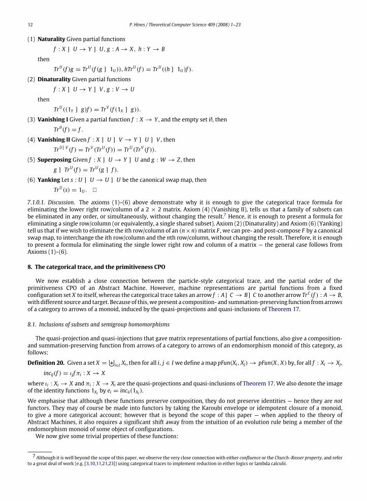
12 P. Hines / Theoretical Computer Science 409 (2008) 1–23
(1) Naturality Given partial functionsf : X ] U → Y ] U, g : A→ X, h : Y → B
then
TrU(f )g = TrU(f (g ] 1U)), hTrU(f ) = TrU((h ] 1U)f ).
(2) Dinaturality Given partial functionsf : X ] U → Y ] V , g : V → U
then
TrU((1Y ] g)f ) = TrV (f (1X ] g)).
(3) Vanishing I Given a partial function f : X → Y , and the empty set ∅, then
Tr∅(f ) = f .
(4) Vanishing II Given f : X ] U ] V → Y ] U ] V , then
TrU]V (f ) = TrV (TrU(f )) = TrU(TrV (f )).
(5) Superposing Given f : X ] U → Y ] U and g : W → Z , then
g ] TrU(f ) = TrU(g ] f ).
(6) Yanking Let s : U ] U → U ] U be the canonical swap map, then
TrU(s) = 1U . �
7.1.0.1. Discussion. The axioms (1)–(6) above demonstrate why it is enough to give the categorical trace formula foreliminating the lower right row/column of a 2 × 2 matrix. Axiom (4) (Vanishing II), tells us that a family of subsets canbe eliminated in any order, or simultaneously, without changing the result.7 Hence, it is enough to present a formula foreliminating a single row/column (or equivalently, a single shared subset). Axiom (2) (Dinaturality) and Axiom (6) (Yanking)tell us that if wewish to eliminate the ith row/column of an (n×n)matrix F , we can pre- and post-compose F by a canonicalswap map, to interchange the ith row/column and the nth row/column, without changing the result. Therefore, it is enoughto present a formula for eliminating the single lower right row and column of a matrix — the general case follows fromAxioms (1)–(6).
8. The categorical trace, and the primitiveness CPO
We now establish a close connection between the particle-style categorical trace, and the partial order of theprimitiveness CPO of an Abstract Machine. However, machine representations are partial functions from a fixedconfiguration set X to itself, whereas the categorical trace takes an arrow f : A]C → B]C to another arrow TrC (f ) : A→ B,with different source and target. Because of this,wepresent a composition- and summation-preserving function fromarrowsof a category to arrows of a monoid, induced by the quasi-projections and quasi-inclusions of Theorem 17.
8.1. Inclusions of subsets and semigroup homomorphisms
The quasi-projection and quasi-injections that gave matrix representations of partial functions, also give a composition-and summation-preserving function from arrows of a category to arrows of an endomorphism monoid of this category, asfollows:
Definition 20. Given a set X =⊎i∈I Xi, then for all i, j ∈ I we define amap pFun(Xi, Xj)→ pFun(X, X) by, for all f : Xi → Xj,
incij(f ) = ιjfπi : X → X
where ιi : Xi → X and πi : X → Xi are the quasi-projections and quasi-inclusions of Theorem 17. We also denote the imageof the identity functions 1Xi by ei = incii(1Xi).
We emphasise that although these functions preserve composition, they do not preserve identities — hence they are notfunctors. They may of course be made into functors by taking the Karoubi envelope or idempotent closure of a monoid,to give a more categorical account; however that is beyond the scope of this paper — when applied to the theory ofAbstract Machines, it also requires a significant shift away from the intuition of an evolution rule being a member of theendomorphism monoid of some object of configurations.We now give some trivial properties of these functions:
7 Although it is well beyond the scope of this paper, we observe the very close connection with either confluence or the Church–Rosser property, and referto a great deal of work (e.g. [3,10,11,21,23]) using categorical traces to implement reduction in either logics or lambda calculii.

P. Hines / Theoretical Computer Science 409 (2008) 1–23 13
Lemma 21. (1) The family {incij} preserves compositions, so incjk(g)incij(f ) = incik(gf ) and hence incii is a semigrouphomomorphism.
(2) ei is idempotent, and ejei = 0X for all i 6= j ∈ I .(3) Given a summable family {fa : Xi → Xj}a∈A, then {incij(fa)}a∈A is also summable, and incij
(∑a∈A fa
)=∑a∈A incij(fa).
(4)∑i∈I ei = 1X .
(5) Given an arrow F : X → X written in matrix form as F =(fij)i,j∈I , where fij = πiF ιj : Xj → Xi for all i, j ∈ I , then
incji(fij) = ejfjiei, and∑i,j∈I ejfjiei = F .
(6) Given arbitrary η : X → X, then eiη ≺ η and ηei ≺ η for all i ∈ I .
Proof. (1) Given f : Xi → Xj, and g : Xj → Xk, then
incjk(g)incij(f ) = ιkgπjιjfπi = ιjg1Xj fπi = ιkgfπi = incij(gf ).
Hence incii is a semigroup homomorphism.(2) As incii is a semigroup homomorphism,
eiei = incii(1Xi)incii(1Xi) = incii(1Xi1Xi) = incii(1Xi) = ei.
Also, eiej = ιiπiιjπj = ιi0Xπj = 0X , by definition of quasi-projections and quasi-inclusions.(3) Both summability of {incij(fa)}a∈A and incij(
∑a∈A(fa)) =
∑a∈A incij(fa) follow from distributivity of composition over
summation:
incij
(∑a∈A
(fa)
)= ιi
(∑a∈A
fa
)πi =
∑a∈A
ιifaπi =∑a∈A
incij(fa).
(4) By definition,∑i∈I ei =
∑i∈I incii(1Xi) =
∑i∈I ιiπi = 1X .
(5) By definition of matrix representations, fij = ιiFπj, and so incji(fij) = πiιiFπjιj = eiFej. Therefore,∑i,j∈I
incji(fij) =∑i,j∈J
eiFej =
(∑i∈I
ei
)F
(∑j∈I
ej
)= 1XF1X = F .
(6) This follows from the definition of the primitiveness ordering and the observation that ei is a partial identity on a subsetof X , since ei(x) = x for all x ∈ dom(ei) = im(ei). Hence ηei(x) is defined implies that η(x) is defined, and η(x) = ηei(x),so ηei ≺ η. Similarly for eiη. �
8.2. Embedding traces into monoids
Wewish tomake a strong connection between the particle-style trace onpartial functions, and the primitiveness relation.However, as the primitiveness relation compares elements of the same endomorphism monoid in a category, we requirethe following definition:
Definition 22. Given a partial function F : X → X , where X = A ] B, we define the resolution ResB(F) of F as
ResB(F) = incAA(TrB(F)) : X → X
where incAA : pFun(A, A)→ pFun(X, X) is as given in Definition 20.Diagrammatically,
X
πA
��
ResB(f ) // X
ATrB(f )
// A
ιA
OO
The terminology ‘Resolution’ above comes directly from Girard’s Geometry of Interaction series of papers [16,17]. Weemphasise that Girard’s ‘resolution formula’ has long been known to be an example of a categorical trace (we refer to [9] foran overview); our embedding of a trace into a monoid is close to the way Girard originally presented his resolution formula.
Lemma 23. (1) Given F : A ] B→ A ] B as above, then
ResB(F) =∞∑i=0
eAF(eBF)ieA =∞∑i=0
eA(FeB)iFeA
where eA, eB are the partial identities on X given in Lemma 21.

14 P. Hines / Theoretical Computer Science 409 (2008) 1–23
(2) Given F : ]i∈IXi → ]i∈IXi, then
ResXp(ResXq(F)) = ResXq(ResXp(F)) = ResXp]Xq(F) ∀p, q ∈ I.
Given the importance of this property in the following sections, we refer to it as the confluence property for resolution.
Proof. (1) Let us write F =(f11 f12f21 f22
)where the components fij are as in Theorem 17. Then
incAA(TrB(F)) = incA
(f11 +
∞∑i=0
f12 f i22f21
).
However, by definition of the matrix components
incAA(TrB(F)) = incA
(πAF ιA +
∞∑i=0
πAF ιB(πBF ιB)iπBF ιA
)and by definition of incAA : End(A)→ End(X),
ResB(F) = ιA
(πAF ιA +
∞∑i=0
πAF ιB(πBF ιB)iπBF ιA
)πA.
By distributivity of composition over summation,
ResB(F) = eAFeA +∞∑i=0
eAF ιB(πBF ιB)iπBFeA
and expanding out the summation gives
ResB(F) = eAFeA + eA(FeB)FeA + eA(FeB)2FeA + eA(FeB)3FeA + · · · .
Therefore ResB(F) =∑∞
i=0 eAF(eBF)ieA =
∑∞
i=0 eA(FeB)iFeA as required.
(2) This follows from Axiom (4) (Vanishing II) for a categorical trace (Theorem 19), and the fact that inc( ) preserves bothcomposition and summation. �
8.3. The particle-style trace and Abstract Machines
Wenow consider the interaction of the tracewith themachine semantics, and primitiveness CPO, of an AbstractMachine.The first, almost immediate, result is closure of both the machine semantics and the cycle-free semantics are closed underthis operation.
Theorem 24. LetM = (X,P ) be an A.M. where X = A] B. Then both the machine semantics [M] and the cycle-free semantics[[M]] are closed under ResB( ).
Proof. • Closure of the machine semantics Let η ∈ [M] be an arbitrary representation. By Lemma 23, ResB(η) =∑∞
i=0 eAη(eBη)ieA. Therefore, ResB(η)(x) = y implies that there exists some K ≥ 0 such that y = eAη(eBη)K eA(x).
However, eA and eB are partial identities on X , so y = ηK+1(x), and hence ResB(η) is a representation satisfyingResB(η) ≺ η.• Closure of the cycle-free semantics Let η ∈ [[M]] be a cycle-free representation. We have seen that ResB(η)(x) = y =ηN(x), for some N > 0. By definition of cycle-freeness, ηK (x) 6= x, for all x ∈ X and K > 0. Hence, ResB(η)(x) 6= x for allx ∈ X , and so ResB(η) is cycle-free. �
As well as the closure of both themachine semantics and the cycle-free semantics under the particle-style trace, we nowdemonstrate that the particle-style trace acts like the computation of a supremum. However, this is a general result aboutmachine semantics, and the order-theoretic result is a special case. We first require some definitions:
Definition 25 (Generalised Down-closure, Down-closure in a Subset). LetM = (X,P ) be an Abstract Machine, and let η ∈[M] be an arbitrary representation. We define the generalised down-closure of η, denoted η ↓ to be the set
η ↓= {µ ∈ [M] : µ ≺ η}.
We emphasise that in general, this is not an order-theoretic definition. However, when η is cycle-free, this is exactly theorder-theoretic down-closure of η in the CPO ([[M]],≺).Now let the configuration set be divided as X = A ] B, and let η be an arbitrary representation, as before. We define the
generalised down-closure of η in A to be the set
η ↓(A)= {µ ≺ η : dom(µ) ⊆ A ⊇ im(µ)}.
Note that this may be a subset of the cycle-free semantics, even when η itself is not cycle-free.

P. Hines / Theoretical Computer Science 409 (2008) 1–23 15
Lemma 26. Let M = (X,P ) be an arbitrary Abstract Machine, where X = A ] B. The following properties of generaliseddown-closure are immediate:(1) [M] = P ↓(2) η ↓(X)= η ↓, for all η ∈ [M].(3) In general, there does not exist some µ such that [[M]] = µ ↓.(4) In general, η ↓(A) ∪ η ↓(B) 6= η ↓(A]B).Proof. (1) and (2) are immediate from the definition. (3) follows since only the primitive evolution is more primitive thanevery cycle-free representation, and so this identity only holds for cycle-free machines. For (4), a necessary and sufficient
condition for η ↓(A) ∪ η ↓(B)= η ↓(A]B) is that the matrix representation of η is of the form η =(η1 00 η2
): A ] B →
A ] B. �
We now establish the connection between the categorical trace, and generalised down-closure:Theorem 27. LetM = (X,P ) be an arbitrary Abstract Machine and let X = A ] B. Then for all η ∈ [M],(1) ResB(η) ∈ η ↓(A)(2) µ ≺ Res(B)(η), for all µ ∈ η ↓(A).Proof. (1) We have seen in Theorem 24 that ResB(η) ≺ η. It is also immediate that the domain and image of ResB(η) arecontained in A ⊆ X . Hence ResB(η) ∈ η ↓(A).
(2) Consider arbitrary µ ∈ η ↓(A). We will demonstrate that for all µ(a) = a′, there exists some L > 0 such thatµ(a) =
(ResB(η)
)L(a), and hence µ ≺ ResB(η).
As µ ≺ η, there exists some K > 0 such that µ(a) = ηK (a). Now denote the partial identities on the subsets A and Bby eA and eB respectively, as in Definition 20. It is immediate that eA = eB = 1X , so we may write
µ(a) = (eA + eB)η(eA + eB)η(eA + eB) . . . (eA + eB)η(eA + eB).However, eAeB = 0X = eBeA, so we may simplify this expression as
µ(a) = eγ0ηeγ1ηeγ2 . . . eγK−1ηeγK where γi ∈ {A, B} ∀0 ≤ i ≤ K .
By the assumption that µ ∈ η ↓(A), we know that α0 = A = αK . Now consider the remaining αi, for 0 < i < K . If theseare all equal to B, then µ(a) = ResB(η)(a), since from Lemma 23, ResB(η) = eAηeA + eAηeBηeA + eAηeBηeBηeA + · · · .Now consider the case where the αi are not all equal to B. Then we may write µ(a) asµ(a) = eA(ηeB)K1ηeA(ηeB)K2ηeA . . . eA(ηeB)KLηeA
where Kj ≥ 0, for all 1 ≤ j ≤ L.Using the idempotency of eA, we rewrite this asµ(a) = eA(ηeB)K1ηeAeA(ηeB)K2ηeA . . . eA(ηeB)KLηeA
and bracket, to getµ(a) = (eA(ηeB)K1ηeA)(eA(ηeB)K2ηeA) . . . (eA(ηeB)KLηeA).
Now compare these bracketed terms with the formula ResB(η) = eAηeA + eAηeBηeA + eAηeBηeBηeA + · · · . We deducethat
µ(a) = (ResB(η))L(a)and hence, as a is an arbitrary member of the domain of µ, we deduce that µ ≺ ResB(η), as required. �
The process of writing µ(a) = a′ as µ(a) = ResB(η)(a) = a′ is illustrated in Fig. 6. We emphasise that although wehave used an analogue of down-closure, and a relation that is a partial order in certain special cases, Theorem 27 itself is notsimply an order-theoretic result. The order-theoretic interpretation arises as a special case:Corollary 28. LetM and η be as above, and further assume that the generalised down-closure of η in A is contained within [[M]].Then η ↓(A) contains its supremum, and ResB(η) = Sup(η ↓(A)).Proof. This follows simply from the fact that ≺, when restricted to cycle-free representations, is a partial order, and fromthe definition of the supremum. Note that this result holds even when η itself is not cycle-free. �
A special case of Corollary 28 above now allows us to write the top element of the black box semantics in terms of acategorical trace, rather than (as in Corollary 15) in terms of the transitive closure:Corollary 29. LetM = (X,P ) be an A.M., with boundary∆M and interior OM . Then the black box semantics is given by
(|M|) = {ResOM (η) : η ∈ [M]}
and the top element of the black box semantics satisfiessup((|M|)) = ResOM (P ).
Proof. Recall from Definition 5 that X = ∆M ] OM , and – as an immediate consequence of their definition – black boxrepresentations are cycle-free. The proof is then almost trivial from Corollary 28. �

16 P. Hines / Theoretical Computer Science 409 (2008) 1–23
Fig. 6. Theorem 27, diagrammatically.
The trace and the transitive closure. Recall fromCorollary 15 that the top element of the black box semantics has an (arguablymuch simpler) expression in terms of the transitive closure of the primitive evolution. The natural question is then whetherthere is any advantage to using the trace formalism to describe this element? We now show (by example, although themethods are general) that the abstract properties of the trace – in particular, the confluence, or vanishing II property –have non-trivial consequences. Precisely, we use the categorical trace to describe algebraic models of space-bounded Turingmachines, and show that the confluence property of the trace corresponds to compositionality of these models.
9. A sample application — space-bounded Turing machines
Using the tools developed in the previous sectionswe now study space-bounded Turingmachines.We choose this examplefor a number of reasons: algebraic models already exist and so provide a good test case. There are also notions of bothconditional iteration and compositionality, and there is also the (informal) idea that universal computation arises as a limitingprocess, as we let the allowed tape length tend to infinity. Even in the bounded case, however, they are decidedly non-trivial structures, and the question of whether the deterministic and non-deterministic versions can perform the samecomputations (the ‘bounded P = NP?’ question) remains an outstanding open problem.Our claim is that, once we have described a bounded Turing machine as an A.M., by giving the configurations, primitive
evolution, and boundary, the usual algebraic models arise in a routine way, as a consequence of Theorem 27. A descriptionof composition and proofs of properties such as associativity are also much easier, as simple properties of the categoricaltrace.
9.1. Space-bounded Turing machines, definitions and dynamics
We assume familiarity with Turing machines, and refer to [19] for a good exposition. Informally, a bounded Turingmachine is then a Turing machine whose operating tape is restricted to the length of the input word.8For a more formal definition, we follow the conventions of [24], based on the conventions of [7] for read-only Turing
machines. The distinction with other conventions, such as [19], is that the machine head of the space-bounded Turingmachine is assumed to be on the boundary of cells on the tape (i.e. between pairs of adjacent cells) rather than pointingat a single cell. However, the translation between the two conventions is relatively straightforward.
Definition 30. A bounded Turing machine, or BTM, T is specified by the following data:
• a set A of alphabet symbols.• a set S of state ormachine head labels.• a direction indicator function dir : S → {left, right}. that is used to partition the state set into left-moving and right-moving states by L = dir−1(left) and R = dir−1(right). Note that Q ∼= L] R, so L∩ R = ∅, and determinism is preserved.• a (partial) transition function F : A× L ] R× A→ L× A ] A× R. This may be given in matrix form as
F =
(frl fllfrr flr
)with the intuition that (for example) the component frl : A× L→ R× A describes the computations that start with themachine head on the rhs of a cell, and finish with the machine head on the lhs of the same cell.
It is possible to give an explicit description of the evolution over time of a space-bounded Turingmachine from the data givenabove, as in [24]. However, we will give this in the language of A.M.s and describe configurations and a primitive evolutionrule.
8We distinguish this concept from linear-bounded Turing machines, whose operating tape is a linear function of the input word. Although it is a classictheorem of complexity theory that the two distinct classes of automata recognise the same formal languages, as A.M.s they are very different devices.

P. Hines / Theoretical Computer Science 409 (2008) 1–23 17
Fig. 7. The anatomy of a bounded Turing machine.
9.2. Space-bounded Turing machines as Abstract Machines
It is implicit in the above definition that
(1) Ordering of the Cartesian product is used to describe position of the machine head. For example, the set S × A describesthe situationwhere themachine head is to the left of a tape cell, whereas A×S describes the situationwhere themachinehead is to the right of a tape cell.
(2) The transition function describes the behaviour of the BTM on a tape of length 1.(3) The ‘left-moving’ and ‘right-moving’ states behave exactly as their names imply, so a machine head with a left-movinglabel will move 1 step to the left, and similarly for right-moving states.
(4) (The principle of locality) The behaviour of F on a tape of length n = a + b can be deduced from the behaviour of Fon tapes of length a, b respectively, via the principles that (i) the action of a (bounded) Turing machine is entirely local,and (ii) this local action uniquely determines the global action of the machine.
9.2.0.2. Convention. In the following subsections, wewill elide the Cartesian product symbol, andwrite (for example) AiSBjfor the set Ai × S × Bj. This is in order to simplify notation and diagrams, and the intended meaning is hopefully clear. Wewill not adopt this convention for Cartesian products of functions, to avoid notational confusion with function composition.
9.2.0.3. Configurations of space-bounded Turingmachines. From (3) above, we see that given a bounded TuringmachineT , we need to treat ‘T , with a tape of length n’ as a different A.M., for each n ∈ N.We denote these distinct AbstractMachinesby Tn. From 1. above, we may then write down the configurations of Tn, as Xn =
⊎ni=0 S
n−iAS i.Therefore, for example, the machine shown in Fig. 7 is in configuration (aba, s, acba) ∈ A3SA4 ⊆ X7.
9.2.0.4. Left and Right moving states. We formalise the intuition of left- and right-moving states in this language ofconfigurations, by stating that for a configuration x which is a member of the subset AiLAj, the next configuration (whenthis exists) will be a member of Ai−1SAj+1 (note that this is not a definition, but is a consequence of the description of theprimitive evolution, below).This allows us to identify the extremal configurations of Tn as the subset Q × An ] An × Q . We will consider these9 as
the boundary∆Tn(Xn).
9.2.0.5. Evolutions of space-bounded Turingmachines. From (2), we have seen that the transition function describes thebehaviour of T on a tape of length 1. We therefore wish to write down a primitive evolution, as a partial function from X1 toitself. Given that
X1 = AS ] SA = A(L ] R) ] (L ] R)A = AL ] AR ] LA ] RA.
We may use the inclusion functions of Definition 20, and define the primitive evolution as P1 = inc(F ) : X1 → X1. Fromthe connection between the inclusion functions and matrix representations, we may write this in matrix form as
P1 =
0 0 0 0frr 0 0 flrfrl 0 0 fll0 0 0 0
: AL ] AR ] LA ] RA→ AL ] AR ] LA ] RA.
9 Strictly, the extremal configurations form a subset of the boundary. However, from the description of the evolution, this subset is guaranteed to containall boundary elements that are within the domain or the image of some representation. The other ‘boundary elements’ that are not within the domain orimage of any representation play no part in any sensible description of the action of a bounded Turing machine (see Definition 5 for this distinction).

18 P. Hines / Theoretical Computer Science 409 (2008) 1–23
It is immediate that P 21 = 0X1 , so T1 is a black box machine.10 Given that most entries of this matrix are zero, we draw the
non-zero entries in diagrammatic form:
LA ALfrl
kk
frr��
RAflr ++
fll
VV
AR
We now need to interpret (3) above in our language of configurations and representations, in order to give the primitiveevolution of Tn, for arbitrary n > 1. We interpret 3(i). as saying that, given a computation b ;a of Tp, and a word w ∈ Aq,thenwb ;wa and bw ;aw are computations of Tp+q. In terms of representations, we say that, for all η ∈ [Tp] andµ ∈ [Tq],
1Aq × η, µ× 1Ap ∈ [Tp+q].
We then interpret 3(ii) as saying that the primitive evolution of Tp+q is exactly the sum of the primitive evolutions of Tp andTq. That is Pp+q ∈ [Tp+q] is given by
Pp+q = 1Aq × Pp + Pq × 1Ap .
Wemay then write down the primitive evolution for Tn as the sum of the primitive evolutions on the individual cells, as
Pn =n∑i=1
1i−1A × P1 × 1An−i+1 .
In general, this is a (2(n+ 1)× 2(n+ 1))matrix. The primitive evolution when n = 2 is
P2 : A2L ] A2R ] ALA ] ARA ] LA2 ] RA2 → A2L ] A2R ] ALA ] ARA ] LA2 ] RA2
given by
P2 =
0 0 0 0 0 0
1A × frr 0 0 1A × flr 0 01A × frl 0 0 1A × fll 0 00 0 frr × 1A 0 0 flr × 1A0 0 frl × 1A 0 0 fll × 1A0 0 0 0 0 0
.Again, since most entries of this matrix are zero (although it is not nilpotent in general, so T2 is not a black box machine), itis reasonable to draw the non-zero entries graphically:
LA2 ALAfrl×1
kk
frr×1
��
A2L1×frlkk
1×frr��
RA2flr×1 ++
fll×1
UU
ARA1×flr ++
1×fll
VV
A2R
and in general, for the primitive evolution Pn of Tn, we draw the diagram
LAn ALAn−1jj
��
· · ·ll An−1LAjj
��
AnLll
��RAn
,,
VV
ARAn−1**
UU
· · · An−1RA**tt
UU
AnR
where the labels on the arrows may be deduced by the context.Readers familiar with the Geometry of Interaction or Int construction will recognise this as a diagrammatic description
of the composition given by the (particle-style) Int construction — the above diagram appears in almost exactly this formin [32]. There is indeed a very close connection between the GoI construction and notions of composition for A.M.s — webriefly consider this in Section 10.
10 It is possible to consider a more general transition function for a bounded Turing machine, where the transition function on a tape of length 1 doesnot describe a black box machine. This situation is considered in an appendix to [24], together with a translation between the two cases, given by theparticle-style categorical trace.

P. Hines / Theoretical Computer Science 409 (2008) 1–23 19
9.3. Algebraic models of space-bounded Turing machines
We now consider algebraic models of space-bounded Turing machines, as defined in [24], and show that an ‘algebraicmodel’ of Tn is exactly the top element of the black box semantics (|T |). Hence, it may be given directly, by using the formulaof Definition 22 to trace out interior configurations, as in Corollary 29.
Definition 31. Let T = (A, S, dir,F ) be as given in Definition 30, and letPn be the primitive evolution for Tn. Then 4 partialfunctions, known as the computation relations for Tn, are defined in [24] as follows:
• [← n−] : AnL→ LAn given by
l′v = [← n−](ul) if and only if l′v ;ul
• [� n] : RAn → LAn given by
l′v = [← n−](ru) if and only if l′v ;ru
• [n �] : AnL→ AnR given by
vr = [← n−](ul) if and only if vr ;ul
• [−n→] : RAn → AnR given by
vr ′ = [← n−](ru) if and only if vr ′ ;ru.
We have already seen that T1 is a black box machine, so we may write down the computation relations for T1 as
[← n−] = frl [� n] = fll[−n �] = frr [n→ ] = flr .
In what follows, we abuse notation, and (for example) refer to the computation relation [← n−] : Xn → Xn when in factwe are working with the image of [← n−] : AnL→ LAn under the appropriate inc : hom(AnL, LAn)→ hom(Xn, Xn) functionof Definition 20. This is for clarity and (since the inc( ) functions are composition- and summation- preserving) the precisemathematical statements are immediate.
Theorem 32. Let Tn be a bounded Turing machine, as above, with primitive evolution Pn. Then
(1) Each computation relation is a black box representation of Tn.(2) The sum of the computation relations is the top element>n of (|Tn|) (equivalently, the computation relations arise as a matrixrepresentation of this top element).
(3) We may calculate>n from the primitive evolution by tracing out the interior configurations, by
>n = ResO(Xn)(Pn).
(4) We may calculate>p+q from>p and>q respectively, as
>p+q = ResApSAq(>p × 1Aq + 1Ap ×>q).
Proof. (1) By definition of machine representations in terms of the ;relation, the computation relations are machinerepresentations. Also, since their respective domains and images are contained in the boundary,∆Tn(Xn), they are blackbox representations.
(2) The identity S = L ] R implies that the computation relations have distinct domains (and images), and are summable.Also, every boundary configuration within the domain of the primitive evolution is within the domain of this sum (bythe ‘if and only if’ in the definition of the computation relations). Therefore, as the primitiveness relation reduces to theinclusion ordering of partial functions, this sum is the top element of the black box semantics,>n ∈ (|Tn|).Finally, the computation relations arise as matrix components of a representation of this element via Theorem 17.
(3) The actual calculation of this top element (& hence the usual algebraic models of bounded Turing machines) followsfrom Corollary 29 of Theorem 27. It is interesting to draw this diagrammatically using the conventions of Section 9.2 —we have ringed the subspaces to be eliminated by the particle-style trace:
This gives a good graphical representation of the construction of>n as ‘eliminating all subspaces where feedback mayoccur’.

20 P. Hines / Theoretical Computer Science 409 (2008) 1–23
The construction of the computation relations for Tn then becomes a routine, albeit non-trivial, application of theResolution formula. For n = 2, a straightforward application of the particle-style trace (as the Resolution formula)gives:
P2 =
0 0 0 0 0 0
1A × frr 0 0 1A × flr 0 01A × frl 0 0 1A × fll 0 00 0 frr × 1A 0 0 flr × 1A0 0 frl × 1A 0 0 fll × 1A0 0 0 0 0 0
ResASA=⇒
0 0 0 0 0 0T 0 0 0 0 U0 0 0 0 0 00 0 0 0 0 0V 0 0 0 0 W0 0 0 0 0 0
= >2where• T = (1A × frr)+ (1A × flr)
∑∞
K=0((frr × 1A)(1A × fll))K (frr × 1A)(1A × frl)
• U = (1A × flr)∑∞
K=0((frr × 1A)(1A × fll))K (flr × 1A)
• V = (frl × 1A)∑∞
K=0((1A × fll)(frr × 1A))K (1A × frl)
• W = (fll × 1A)+ (frl × 1A)∑∞
K=0((1A × fll)(frr × 1A))K (1A × fll)(flr × 1A).
It may be checked that this matches the computation relations for T2, as derived via a brute-force calculation based oncrossing number arguments, in [24].
(4) From above, it may be seen that direct calculation of the computation relations becomes very complex, very quickly.Fortunately,>p+q may be calculated from>p and>q, as we now demonstrate:Recall the definition of Pn as Pn =
∑ni=1 1
i−1A × P1 × 1An−i+1 . From this it is immediate that
Pp+q = (Pp × 1Aq)+ (1Ap × Pq).
By (2) above,
>p+q = ResO(Xp+q)(Pp+q) = ResO(Xp+q)((Pp × 1Aq)+ (1Ap × Pq)).
However, by definition O(Xp+q) = U ] V ]W where
U = O(Xp)× Aq, V = ApSAq,W = Ap × O(Xq).
Then, using the confluence property of Lemma 23,
>p+q = ResU]V]W (Pp+q) = ResU]V]W ((Pp × 1Aq)+ (1Ap × Pq))
= ResV]W ((>p × 1Aq)+ (1Ap × Pq))
= ResV ((>p × 1Aq)+ (1Ap ×>q))
by basic properties of the categorical trace. Finally, as V = ApSAq
>p+q = ResApSAq((>p × 1Aq)+ (1Ap ×>q))
as required. �
Confluence and compositionality. Note the vital rôle played by the Vanishing II, or confluence property of the trace in provingcompositionality of algebraic models in the above theorem — this is not readily derivable from the description of the topelement of the black box semantics in terms of transitive closure. Given the close connection between confluence in logicalsystems, and compositionality in state machine models, it is very tempting to consider them as two sides of the same coin.
10. Conclusions, discussion, future directions
Hopefully, this paper has demonstrated that real, non-trivial, theory can arise from considering Abstract Machines, andthe interaction of the primitiveness CPO with the particle-style trace. The specific example of a bounded Turing machinewas chosen, because of the reasons given in Section 9 – and because the author is familiar with the previous construction ofalgebraic models [24] – however, the theory was not constructed sôlely with this application in mind — Abstract Machinesare ultimately simply sets with a discrete notion of causality.In terms of future directions, the refereeing process for this paper overlapped with the acceptance of a sequel paper,
[26]. The key points of this sequel are: (1) the primitiveness CPO is in fact a Scott domain, and connections to models of pureuntyped lambda calculus are considered, (2) the primitive evolution of an AM can be used to divide the configuration set intothe Cartesian product of ‘code’ and ‘data’ sets — purely abstractly, this is a natural way of constructing labelled transitionsystems from unlabelled transition systems, (3) the code-data division need not be unique; rather it has a rich order theorybehind it, and (4) for certain classes of state machines, the split between the Alphabet and State-set is exactly this code-datadivision of the configuration set.There still remain a number of unanswered questions.What is certainlymissing is a general notion of composing Abstract
Machines. The bounded T.M. example given here has a nice description via the principle of locality, Section 9.2; however, itis not immediate how to generalise this to arbitrary abstract machines in other categories, since this principle relies on both

P. Hines / Theoretical Computer Science 409 (2008) 1–23 21
the Cartesian product and the coproduct (i.e disjoint union). A general description of composition, together with how thisinteracts with the order theory presented, would almost certainly lead to a domain-theoretic interpretation of the (particle-style) Geometry of Interaction or Int construction of [1,32].With regard to the Geometry of Interaction construction, Girard’s original system [16,17] (a representation of linear logic
[15]) was based on the Resolution formula, which has been shown to be a particle-style trace. However, shortly after itspublication, this system was re-interpreted in domain-theoretic terms by Abramsky and Jagadeesan [2]. It remains to beshown whether this is directly related to the domain theory provided by the primitiveness partial ordering.The above question is a specific example of a more general question about different types of categorical trace. In [1], a
strong distinction is made between ‘particle-style’ traces, based on iteration, and ‘wave-style’ traces based on fixed-pointconstructions. The canonical example of a particle-style trace is the trace on the category of partial functions (as describedin Definition 18) whereas the canonical example of a ‘wave-style’ trace is the least fixed point in a category of domains. It istherefore highly unexpected that the particle-style trace also has a domain-theoretic interpretation.A further, very natural, categorical approach would be to consider Abstract Machines that live in other categories.
The theory developed in this paper is entirely based within the category of partial functions on sets — extensions tocategories of either partial reversible functions or relations are straightforward, but an account of Abstract Machines withconfigurations/representations taken from the objects/arrows of a general (presumably traced) category remains to be given.A key future generalisation is motivated by the intention of modelling discrete physical systems by Abstract Machines. The
natural direction to take is thus to study ‘quantum Abstract Machines’. However, there are a number of subtleties. We maytake as primitive the idea of applying a unitary (or completely positive) operation to a configuration in Hilbert space (or adensity matrix) — as in either Grover’s algorithm [18], or the quantum Turing machine [13]. This gives a clear notion of bothconfigurations and the primitive evolution. In the finite-dimensional unitary case, we then see that no quantum AbstractMachine may be cycle-free (since for an arbitrary unitary U : H → H , on finite dimensional space, then there exists Nsuch that ‖UN − 1H‖ < ε). However, this is only part of the story. In Grover’s algorithm, a measurement is made (andthe computation terminates) after a fixed number of iterations — this is also the approach taken to halting of QM Turingmachines in [8], and two-way quantum automata in [33]. So, it seems that a (classical) clock that counts the number of stepstaken is an unavoidable part of the configuration space (we refer to [6,27] for such ideas from two different perspectives,including the construction of a particle-style trace from unitary maps). Steps towards a theory of QM Abstract Machineshave been given in [28], but many questions remain to be resolved.
Acknowledgements
The author was raised as a category-theorist, rather than a domain-theorist, and so must acknowledge many usefuldiscussions with peoplemore familiar with this subject, including Samson Abramsky, Bob Coecke, KeyeMartin, and PrakashPanangaden. Thanks are also due to Sam Braunstein, for many helpful discussions on physical justifications for propertiesof Abstract Machines, and to the York non-standard computation group for the many weird and wonderful devices used as‘computingmachines’. Thanks are also due to Samson Abramsky, for the suggestion of studying the GoI systemusing domaintheory, and to Philip Scott for assistance with the logical and categorical theory of the particle-style trace, and discussionsof properties of iteration and halting.Finally, the author wishes to thank Pierre-Louis Curien, the TCS editor responsible for handling this paper for his
assistance, and anonymous referees for suggestions on how to improve presentation and readability.Author’s research was supported by QIP IRC www.qipirc.org (GR/S82176/01).
Appendix A
In this appendix, we demonstrate that in general, most properties relating to cycle-freeness are undecidable.
Proposition 33. It is undecidable when an Abstract Machine is cycle-free, even when the primitive evolution is a computable(partial) function.
Proof. LetM = (X,P ) be an Abstract Machine defined by some Turing machine T . The configurations are the set of allspecifications of the tape contents, together with position and label of the machine head. The primitive evolution is givenby the transition rule for the T.M.This machine may or may not be cycle-free, depending on the properties of the Turing machine T . We now define a new
Abstract MachineMC = (Y ,R). The configurations and primitive evolution are given by :
• (configurations) Y = X × N• (primitive evolution)
R(x, n) ={(P (x), n+ 1) when x is not a halting configuration(x, n) when x is a halting configuration.
It is then immediate that the machineMC is cycle-free exactly whenM, never reaches a halting configuration. However, asM is specified by a Turing machine, this is in general undecidable. �

22 P. Hines / Theoretical Computer Science 409 (2008) 1–23
Not only is it in general undecidable whether a representation or abstract machine is cycle-free, the same applies toeither the sum or composite of cycle-free representations:
Theorem 34. It is in general undecidable whether the sum or composite of cycle-free representations is also cycle-free.
Proof. We prove this result for the sum of cycle-free representations. The proof for the composite is similar.Let M = (X,P ) be an Abstract Machine defined by some Turing machine T . The configurations are the set of allspecifications of the tape contents, together with position and label of the machine head. The primitive evolution is givenby the transition rule for the T.M. We assume that T is given as the natural generalisation of the space-bounded machinesgiven in Section 9.1, so each state (i.e. label on the machine head) is either left-moving or right-moving, and the direction ofmovement is uniquely determined by the label on the machine head.We split the primitive evolution into two distinct partial functions: Pl,Pr : X → X . These are given by restricting
the domain of P to configurations with a left-moving state, and right-moving state, respectively. It is then immediate thatPl is a cycle-free representation, and similarly for Pr . However, by construction P = Pl + Pr and, as demonstrated inProposition 33, it is undecidable whether P is cycle-free. �
Appendix B
Much of this paper is about studying arbitrary Abstract Machines via the structure of their cycle-free semantics. Thisraises the natural question of how much information the cycle-free semantics of an Abstract Machine provides about theAbstract Machine itself – by considering only the cycle-free semantics, are we missing important structure?Theorem 37 answers this question in the negative; however, we first require some terminology :
Definition 35. Let M = (X,P ) be an Abstract Machine. We say M is fixed-point free when y = P (x) implies x 6= y.Similarly, we say that a representation η ∈ [M] is fixed-point free when η(x) 6= x, for all x ∈ X . Clearly, a fixed-pointfree machine is one where the primitive evolution is fixed-point free. However, it in general, not all representations of afixed-point free machine are themselves fixed-point free.
We emphasise this is not the same concept as cycle-free. A machine is fixed-point free when the primitive evolutionnever returns a configuration to itself in a single step, whereas it is cycle-free when the primitive evolution never returns aconfiguration to itself no matter how long the computational path.For an arbitrary Abstract MachineM, we can define the ‘largest’ fixed-point free analogue in a natural way:
Definition 36. LetM = (X,P ) be an Abstract Machine. We define the Abstract MachineMo= (X,P o) to have the same
configuration set, and primitive evolution given by
y = P o(x) ⇔ y = P (x) and y 6= x
i.e. P o is the largest fixed-point free partial function beneath P , with respect to the inclusion ordering of Definition 13.
Intuitively we may describeMo as, ‘M with all cycles of length 1 removed’. Our claim is now that the cycle-free semanticsofM ‘provides enough information’ to reconstruct the machine semantics ofMo. We formalise this as follows :
Theorem 37. Let M = (X,P ) be an Abstract Machine, with cycle-free semantics [[M]] ⊆ pFun(X, X). Then the closure of[[M]] under composition and (partial) summation of partial functions given in Definition 2 is exactly the machine semantics ofMo= (X,P o).
Proof. For an Abstract MachineM, let us consider the set of all pairs SM = {(y, x) : y = P (x) and y 6= x} ⊆ X × X . Clearlythis is the same subset of X × X for bothM andMo, i.e. SM = SMo .
Each pair (y, x) ∈ SM specifies a partial function f(y,x) : X → X , defined by f(y,x)(a) ={y a = xundefined otherwise.
This partial function is trivially cycle-free, so f(y,x) ∈ [[Mo]]. Now consider an arbitrary representation η ∈ [Mo
]. For eachb = η(a), there exists a set of pairs
{(b, xk), (xk, xk−1) , . . . (x2, x1) , (x1, a)} ⊆ S
so
b = f(b,xk)f(xk,xk−1) . . . f(f2,x1)f(x1,a)(a).
Let us call this composite ηa. For distinct a, a′ ∈ dom(η), the partial functions ηa and ηa′ have disjoint domains. Therefore,the family {ηa}a∈dom(η) is summable, and it is immediate that η =
∑a∈dom(η) ηa.
Hence, we have expressed an arbitrary representation η ∈ [Mo] ⊆ [M] in terms of the composite and sum of cycle-free
representations. Note also that by Proposition 4, [Mo] is closed under composition and summation, so all partial functions
derived using these operations are representations of Mo. Finally, it is left as an interesting exercise to show that thisprocedure does not work for any µ ∈ [M] \ [Mo
]. �
The relationship between machinesM andMo has a natural intuitive interpretation in terms of how ‘halting’ is treated, asfollows:

P. Hines / Theoretical Computer Science 409 (2008) 1–23 23
Halting, and fixed-point free machines. For various state machines (e.g. Turing machines and similar), a set of ‘haltingconfigurations’ is required to signal when the result of a computation has been reached. Although some arbitrary set ofconfigurations may be chosen to be ‘halting’ configurations, it is more natural to let halting be defined by the machinebehaviour. There are two immediate possibilities : a configuration hmay be a halting configuration when(1) there is no ‘next configuration’ specified for h.(2) the next configuration after h is again h itself.
Although the distinction is almost trivial, it gives rise to the important unresolved question of how to deal with halting forquantum Turing machines [38] (note also that the ‘halting procedure’ for the iterative trace on quantum systems in [27] isbased on a variant of (1) above). In our terms, by passing from an arbitrary AbstractMachineM to its fixed-point free versionMo, we are translating a machine following (2) into a machine following (1) — i.e. configurations satisfying h = P (h) areforcibly removed to the boundary.
References
[1] S. Abramsky, Retracing some paths in process algebra, in: CONCUR 96, in: Lecture Notes in Computer Science, Springer-Verlag, 1996, pp. 1–17.[2] S. Abramsky, A. Jung, Domain Theory, in: S. Abramsky, D.M. Gabbay, T.S.E. Maibaum (Eds.), Handbook of Logic in Computer Science, vol. III, OxfordUniversity Press, 1994.
[3] A. Abramsky, R. Jagadeesan, New foundations for the geometry of interaction, in: Proc. 7th annual IEEE conf. on Logic in Computer Science, 1992, pp.211–222.
[4] S. Abramsky, E. Haghverdi, P. Scott, Geometry of interaction and linear combinatory algebras, Mathematical Structures in Computer Science 12 (5)(2002).
[5] R. Amadio, P.-L. Curien, Domains and Lambda Calculii, Cambridge University Press, 1998.[6] B. Apolloni, D. de Falco, The clock of a quantum computer, Journal of Physics, A. Mathematical and General 35 (2002) 10033–10051.[7] J.-C. Birget, Basic techniques for two-way finite automata, in: Formal Properties of Finite Automata and Applications, in: LNCS, Springer-Verlag, 1989,pp. 56–64.
[8] E. Bernstein, U. Vazirani, Quantum complexity theory, SIAM Journal on Computing 26 (5) (1997) 1411–1473.[9] R. Blute, R. Cockett, R. Seely, Feedback for linearly distributive categories: Traces and fixed points, Journal of Pure and Applied Algebra 154 (2000)27–69.
[10] R. Blute, P. Scott, Category theory for linear logicians, in: Linear Logic in Computer Science, in: London Math. Soc. Lecture Notes, vol. 316, Camb. U.Press, 2004, pp. 3–64.
[11] V. Danos, L. Regnier, Local and asynchronous β-reduction, in: Proceedings of the Eighth Annual IEEE Symp. on Logic in Computer Science, 1993.[12] B. Davey, H. Priestley, Introduction to Lattices and Order, 2nd ed., Cambridge University Press, 2002.[13] D. Deutsch, Quantum theory, the Church-Turing principle and the universal quantum computer, Proceedings of Royal Society of London A 400 (1985)
97–117.[14] FOLDOC: The free online directory of computing, 1993. http://foldoc.org/, Editor Denis Howe, supported by Imperial College Dept. of Computing.[15] J.-Y. Girard, Linear logic, Theoretical Computer Science 1 (50) (1987).[16] J.-Y. Girard, Geometry of interaction 1, in: Proceedings Logic Colloquium ’88, North-Holland, 1988, pp. 221–260.[17] J.-Y. Girard, Geometry of interaction 2, in: P. Martin Löf, G. Mints (Eds.), Proceedings of COLOG ’88, in: Springer-Verlag Lecture Notes in Computer
Science, vol. 417, 1988, pp. 76–93.[18] L. Grover, A fast quantum mechanical algorithm for database search, in: Proceedings, 28th Annual ACM Symposium on the Theory of Computing,
1996, pp. 212–219.[19] J. Hopcroft, J. Ullman, Automata theory, languages, and computation, Reading, MA, 1979.[20] E. Haghverdi, A categorical approach to linear logic, geometry of proofs and full completeness, Ph.D. Thesis, Univ. Ottawa, 2000.[21] E. Haghverdi, P. Scott, A categorical model for the geometry of interaction, Theoretical Computer Science 350 (2–3) (2006) 252–274.[22] E. Haghverdi, P. Scott, Geometry of interaction and the dynamics of proof reduction: A tutorial (in press).[23] P. Hines, The algebra of self-similarity and its applications, Ph.D. Thesis, Univ. Wales, Bangor, 1997.[24] P. Hines, A categorical framework for finite state machines, Mathematical Structures in Computer Science (13) (2003) 451–480.[25] P. Hines, Physical systems as constructive logics, in: C. Calude, M. Dinneen, G. Paun, G. Rozenberg, S. Stepney (Eds.), Unconventional Computation, UC
2006: York, UK., in: Springer. LNCS, 2006.[26] P. Hines, Machine semantics — from causality to computational models, International Journal of Unconventional Computation 4 (3) (2008) 249–272.[27] P. Hines, P. Scott, Conditional quantum iteration from categorical traces (submitted).[28] P. Hines, Towards a quantum machine semantics, Mathematical Foundations of Programming Semantics, 2007. Invited talk, Available as:
http://www.peterhines.net/downloads/talks/MFPS2007.pdf.[29] J. Isbell, Atomless parts of spaces, Mathematica Scandinavica 31 (1972) 5–32.[30] T. Iwamura, A lemma on directed sets, Zenkoku Shijo Sugaku Danwakai 262 (1944) 107–111 (in Japanese). An English exposition is available in [36].[31] P. Johnstone, The point of pointless topology, Bulletin American Mathematical Society 8 (1) (1983) 41–53.[32] A. Joyal, R. Street, D. Verity, Traced Monoidal categories, Mathematical Proceedings of the Cambridge Philosophical Society (1996) 425–446.[33] A. Kondacs, J. Watrous, On the power of quantum finite state automata, in: Proceedings of the 38th Annual Symposium on Foundations of Computer
Science, FOCS ’97, October 19–22, IEEE Computer Society, 1997.[34] J. Lambek, P. Scott, Introduction to Higher Order Categorical Logic, Cambridge University Press, 1986.[35] E. Manes, M. Arbib, Algebraic Approaches to Program Semantics, Springer-Verlag, 1986.[36] G. Markowsky, Chain-complete p.o. sets and directed sets with applications, Algebra Universalis 6 (1976) 53–68.[37] K. Martin, P. Panangaden, A domain of space-time intervals in general relativity, in: Spatial Representation: Discrete vs. Continuous Computational
models, Dagstuhl Seminar Proceedings, 2005.[38] J. Myers, Can a universal computer be fully quantum? Physical Review Letters 78 (9) (1997) 1823–1824.[39] G. Plotkin, A structural approach to operational semantics, Tech. Rep. DAIMI FN-19, Computer Science Department, Aarhus University, 1981. Also
available as Elsevier EBOOK 1001, Media2book inc., Paris..[40] D. Scott, Outline of a mathematical theory of computation, in: 4th Annual Princeton Conference on Information Sciences and Systems, 1970, pp.
169–176.[41] J. Stoy, Denotational Semantics, the Scott–Stratchey Approach to Programming Language Semantics, MIT press, 1977.[42] A. Troelstra, H. Schwichtenberg, Basic Proof Theory, 2nd ed., Cambridge University Press, 2000.[43] D. Scott, Domains for denotational semantics, in: Proc. 9th Colloquium on Automata, Languages and Programming, in: Lecture Notes In Computer
Science, vol. 140, 1982, pp. 577–613.[44] Z. Silagadze, Zeno meets modern science, Acta Physica Polonica B 36 (2005) 2886–2930.[45] S. Vickers, Topology via Logic, Cambridge University Press, 1989.[46] S. Wolfram, A New Kind of Science, Wolfram Media Inc., 2002.