Machine Learning RL 1

Reinforcement Learning in Partially Observable Environments

Michael L. Littman

Machine Learning RL 2

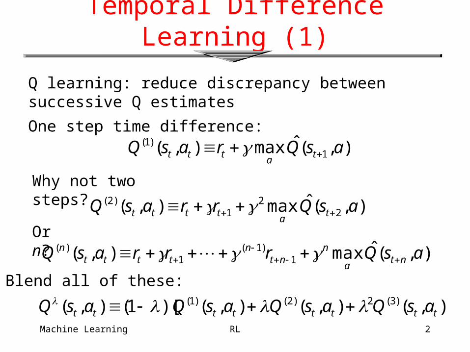
Temporal Difference Learning (1)

),(),(),()[1(),( )3(2)2()1(tttttttt asQasQasQasQ

),(ˆmax),( 1)1( asQrasQ t

attt

Q learning: reduce discrepancy between successive Q estimates

One step time difference:

Why not two steps?

),(ˆmax),( 22

1)2( asQrrasQ t

atttt

Or n?),(ˆmax),( 1

)1(1

)( asQrrrasQ nta

nnt

ntttt

n

Blend all of these:

Machine Learning RL 3

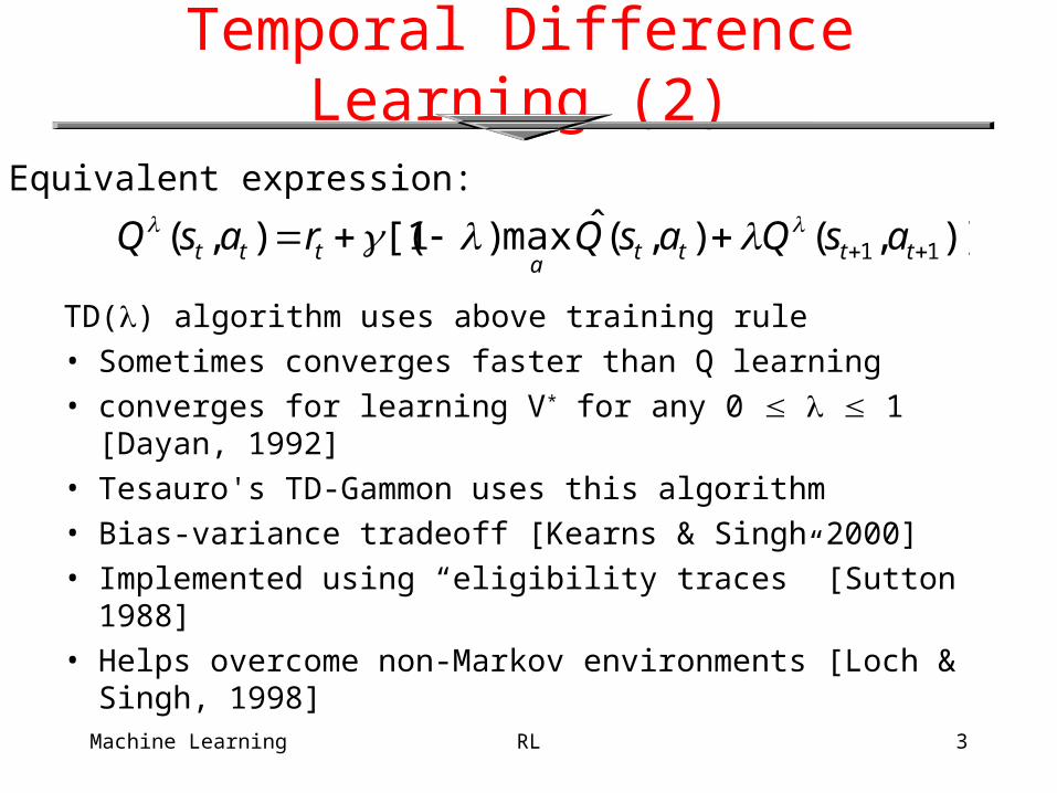
Temporal Difference Learning (2)

TD() algorithm uses above training rule• Sometimes converges faster than Q learning• converges for learning V* for any 0 1 [Dayan,

1992]• Tesauro's TD-Gammon uses this algorithm• Bias-variance tradeoff [Kearns & Singh 2000]• Implemented using “eligibility traces” [Sutton 1988]• Helps overcome non-Markov environments [Loch &

Singh, 1998]

)],(),(ˆmax)1[(),( 11 tttta

ttt asQasQrasQ Equivalent expression:

Machine Learning RL 4

non-Markov Examples

Can you solve them?

Machine Learning RL 5

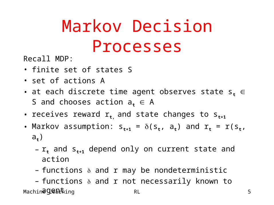
Markov Decision ProcessesRecall MDP:• finite set of states S • set of actions A

• at each discrete time agent observes state st S and chooses action at A

• receives reward rt, and state changes to st+1

• Markov assumption: st+1 = (st, at) and rt = r(st, at)

– rt and st+1 depend only on current state and action

– functions and r may be nondeterministic – functions and r not necessarily known to agent

Machine Learning RL 6

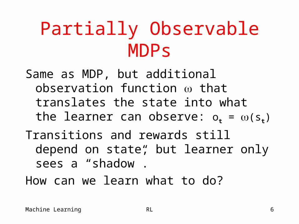
Partially Observable MDPs

Same as MDP, but additional observation function that translates the state into what the learner can observe: ot = (st)

Transitions and rewards still depend on state, but learner only sees a “shadow”.

How can we learn what to do?

Machine Learning RL 7

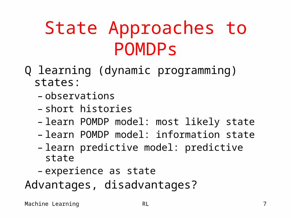
State Approaches to POMDPs

Q learning (dynamic programming) states:– observations– short histories– learn POMDP model: most likely state– learn POMDP model: information state– learn predictive model: predictive state– experience as state

Advantages, disadvantages?

Machine Learning RL 8

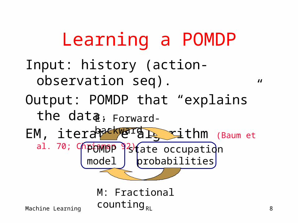
Learning a POMDPInput: history (action-observation seq).

Output: POMDP that “explains” the data.EM, iterative algorithm (Baum et al. 70; Chrisman 92)

state occupationprobabilities

POMDPmodel

E: Forward-backward

M: Fractional counting

Machine Learning RL 9

EM Pitfalls

Each iteration increases data likelihood.Local maxima. (Shatkay & Kaelbling 97; Nikovski 99)

Rarely learns good model.

Hidden states are truly unobservable.

Machine Learning RL 10

Information State

Assumes:

• objective reality

• known “map”

Also belief state: represents location.

Vector of probabilities, one for each state.

Easily updated if model known. (Ex.)

Machine Learning RL 11

Plan with Information StatesNow, learner is 50% here and 50% there

instead of in any particular state.

Good news: Markov in these vectors

Bad news: States continuous

Good news: Can be solved

Bad news: ...slowly

More bad news: Model is approximate!

Machine Learning RL 12

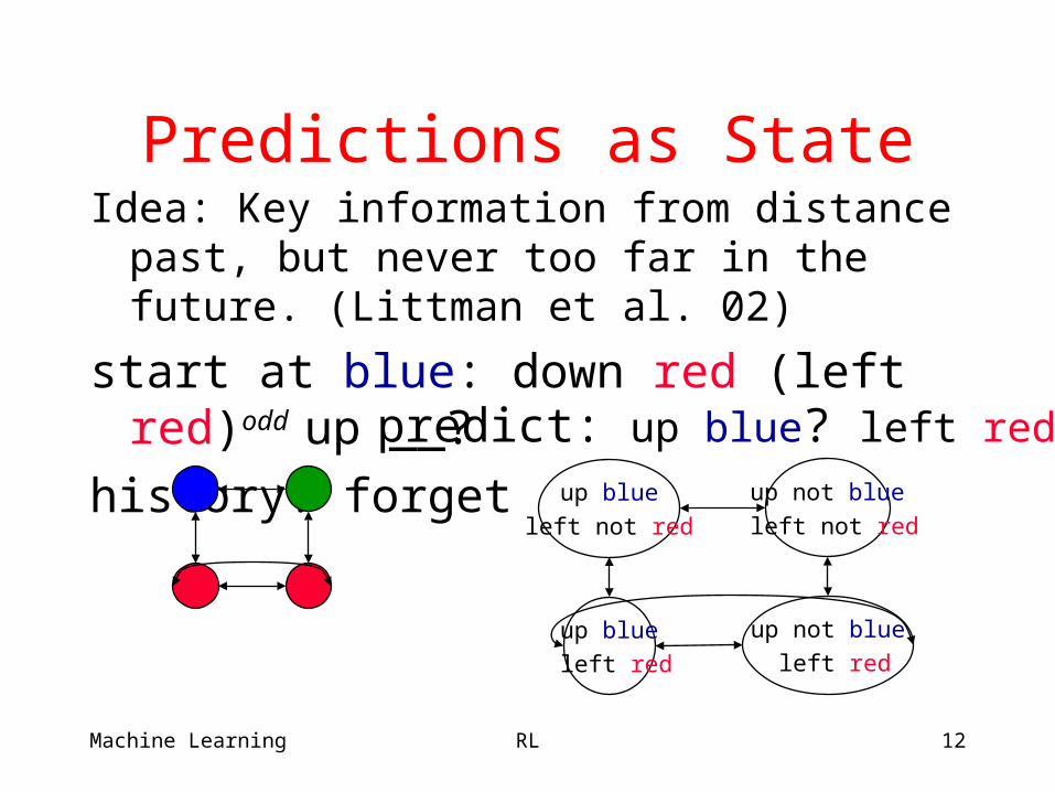
Predictions as StateIdea: Key information from distance past, but

never too far in the future. (Littman et al. 02)

start at blue: down red (left red)odd up __?

history: forget

up blue

left red

up not blue

left not red

up blue

left not red

predict: up blue? left red?

up not blue

left red

Machine Learning RL 13

Experience as State

Nearest sequence memory (McCallum 1995)

Relate current episode to past experience.

k longest matches considered to be the same for purposes of estimating value and updating.

Current work: Extend TD(), extend notion of similarity (allow for soft matches, sensors)

Machine Learning RL 14

Classification Dialog (Keim & Littman 99)

User to travel to Roma, Torino, or Merino?

States: SR, ST, SM, done. Transitions to done. Actions:

– QC (What city?),– QR, QT, QM (Going to X?),– R, T, M (I think X).

Observations:– Yes, no (more reliable), R, T, M (T/M confusable).

Objective:– Reward for correct class, cost for questions.

Machine Learning RL 15

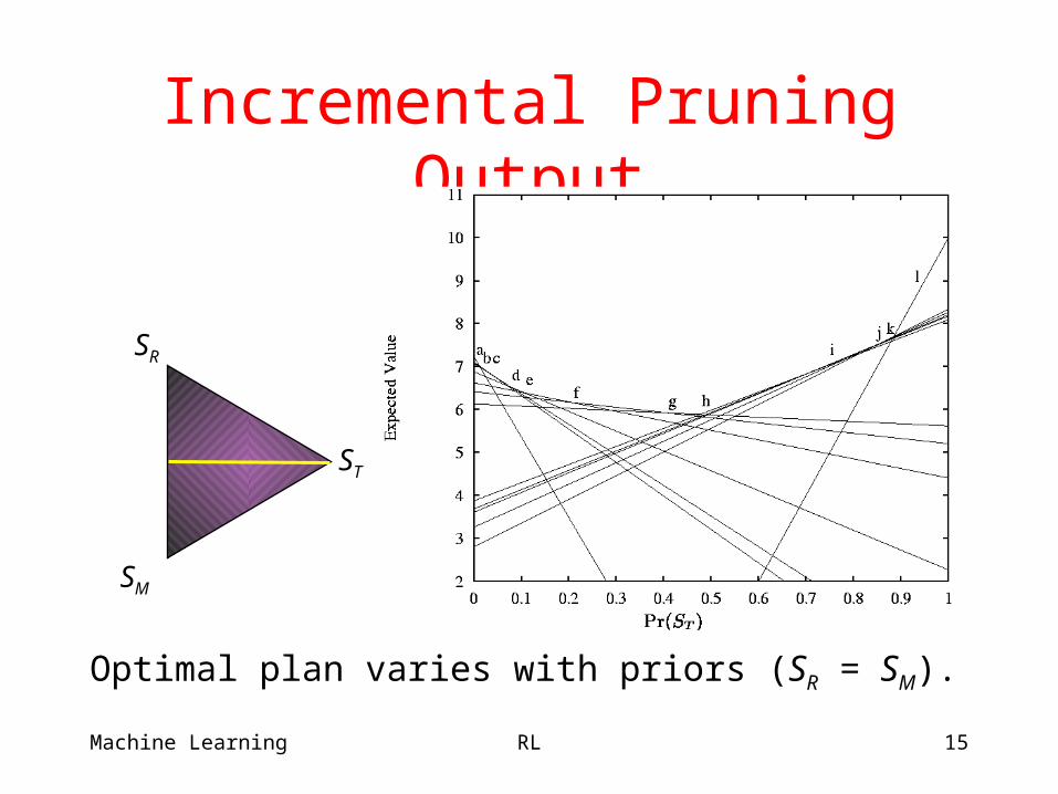
Incremental Pruning Output

Optimal plan varies with priors (SR = SM).

ST

SR

SM

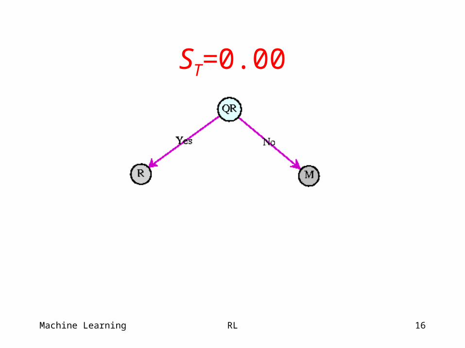
Machine Learning RL 16

ST=0.00

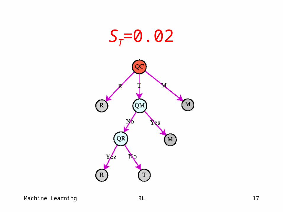
Machine Learning RL 17

ST=0.02

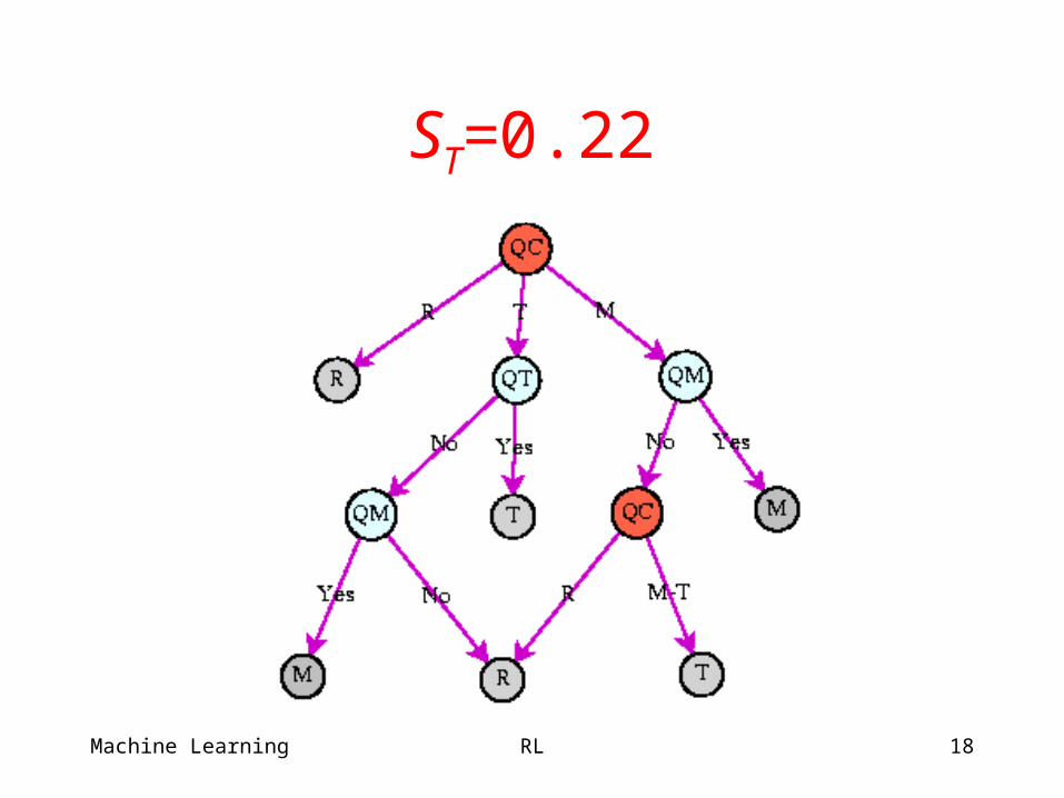
Machine Learning RL 18

ST=0.22

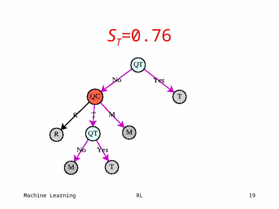
Machine Learning RL 19

ST=0.76

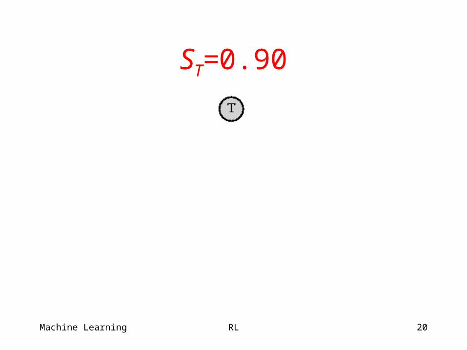
Machine Learning RL 20

ST=0.90

Machine Learning RL 21

Wrap Up

Reinforcement learning: Get the right answer without being told. Hard, less developed than supervised learning.

Lecture slides on web.

http://www.cs.rutgers.edu/~mlittman/talks/• ml02-rl1.ppt• ml02-rl2.ppt