Machine Learning of Timed Automata · Machine Learning of Timed Automata ... Process mining is a...
191
TECHNISCHE UNIVERSIT ¨ AT M ¨ UNCHEN Fakult¨atf¨ ur Informatik Lehrstuhl f¨ ur Bioinformatik Machine Learning of Timed Automata Jana A. Schmidt Vollst¨andiger Abdruck der von der Fakult¨ at f¨ ur Informatik der Tech- nischen Universit¨at M¨ unchen zur Erlangung des akademischen Grades eines Doktors der Naturwissenschaften genehmigten Dissertation. Vorsitzender: Univ.-Prof. Dr. R. Westermann Pr¨ ufer der Dissertation: 1. Univ.-Prof. Dr. B. Rost 2. Univ.-Prof. Dr. St. Kramer Johannes Gutenberg Universit¨at Mainz Die Dissertation wurde am 27.05.2013 bei der Technischen Univer- sit¨ at M¨ unchen eingereicht und durch die Fakult¨ at f¨ ur Informatik am 25.11.2013 angenommen.
Transcript of Machine Learning of Timed Automata · Machine Learning of Timed Automata ... Process mining is a...

TECHNISCHE UNIVERSITAT MUNCHEN
Fakultat fur InformatikLehrstuhl fur Bioinformatik
Machine Learning of Timed Automata
Jana A. Schmidt
Vollstandiger Abdruck der von der Fakultat fur Informatik der Tech-nischen Universitat Munchen zur Erlangung des akademischen Gradeseines
Doktors der Naturwissenschaften
genehmigten Dissertation.
Vorsitzender: Univ.-Prof. Dr. R. Westermann
Prufer der Dissertation:1. Univ.-Prof. Dr. B. Rost2. Univ.-Prof. Dr. St. Kramer
Johannes Gutenberg Universitat Mainz
Die Dissertation wurde am 27.05.2013 bei der Technischen Univer-sitat Munchen eingereicht und durch die Fakultat fur Informatik am25.11.2013 angenommen.


Ich versichere, dass ich diese Dissertation selbstandig verfasst und nur dieangegebenen Quellen und Hilfsmittel verwendet habe.
Munchen, den 17.05.2013

Abstract
This dissertation investigates the applicability of automata in the do-main of process mining. Process mining is a part of machine learning thataims to describe, discover and to predict dynamic systems. It can be usedespecially in the domain of biology and medicine where many processes arestill not fully understood. The main problem here is that the processes arevery complex and that many factors interact with each other. Usually, onetries to model these factors by variables that influence each other. There-fore, a kind of dependency structure of the variables within a specific modelis optimized to best reflect the measured data. In contrast, this work aimsat modeling the variables’ values change without explicitly assuming theinter-dependencies. This aim is achieved by a new type of model, whichis based on automata. Automata are finite state models that are normallyused to express formal grammars, to model and to detect languages thatrely on discrete events. However, we expand the power of automata, as afirst step towards modeling dynamic multivariate processes. Therefore, onepart was to find a method (Prta), which automatically identifies states andtransitions of the given process. This is necessary because usually, the defi-nition of states, i.e., the current characteristics of the system, are not knownor have not been described before. To this end, the states of an automatonare annotated with so-called profiles, which describe the current stage of thesystem. The main idea for the automatic identification of the profiles is toextract frequent patterns of the process variables’ characteristics. Moreover,the time component of the process should also be captured, which is done bythe implementation of clock guards that define in which time frame a changein the states may take place. A subsequent problem is the scalability of theapproach for large data sets. Therefore, a method (Sprta) that uses on-line maximum frequent pattern based clustering is presented. To includeexisting background knowledge, a new type of constraint was developed andalso implemented in the proposed approach (CSprta). Such constraints arebased on the characteristics of the process and basically define the proper-ties of the final states. Lastly, an improvement towards a genuine onlineinduction method is presented (Oprta). It may also detect concept drift inthe underlying system. All of these approaches are evaluated with respect toscalability, accuracy, and, if appropriate, predictability. We hope that thiskind of model may find some applications in biological and medical processmining.

Zusammenfassung
Diese Dissertation beschaftigt sich mit der Frage, ob Automaten fur dasLernen von dynamischen Prozessen anwendbar sind. Der Bereich des soge-nannten ’Process Mining’ als Teil des maschinellen Lernens versucht dieseProzesse zu beschreiben, zu entdecken und auch deren Verlauf vorherzusagen.Besonders in der Biologie und Medizin kann das Anwendung finden, da dortviele Prozesse noch nicht ausreichend verstanden werden. Die Hauptur-sache dafur liegt darin, dass diese Prozesse sehr komplex sind und viele Fak-toren miteinander interagieren. Bis jetzt versuchte man hauptsachlich, dieseFaktoren mittels voneinander abhangigen Variablen und einer Abhangig-keitsstruktur in bestimmten Modellen nachzubilden, so dass die gemessenenDaten moglichst optimal reproduziert werden konnen. Im Gegensatz dazuversucht diese Arbeit die Anderung der Variablenauspragungen zu mod-ellieren, ohne direkt Abhangigkeiten zwischen den Variablen anzunehmen.Dazu wurde ein neues Modell basierend auf Automaten entwickelt. Auto-maten sind endliche Zustandsmaschinen, die hauptsachlich darin Anwen-dung finden, formale Grammatiken zu beschreiben und Sprachen zu model-lieren bzw. zu entdecken, die auf diskreten Ereignissen beruhen. Trotzdemhaben wir in dieser Arbeit, Automaten dahingehend erweitert, dynamis-che multivariate Prozesse abbilden zu konnen (Prta). Dazu war es zuerstnotig, eine Methode zu definieren, die aus den gegebenen Daten automatischZustande des Modells induziert, da solche Zustande, d.h. die derzeitigenEigenschaften des Systems, u.U. nicht bekannt sind oder noch nicht konso-lidiert wurden. Dafur werden die Zustande im Automaten mit sogenanntenProfilen annotiert, die den derzeitigen Zustand des Systems beschreiben.Die zugrunde liegende Idee bei der Identifikation der Zustande und ihrerProfile ist, haufige Muster in den Eigenschaften des Prozesses zu entdecken.Daneben soll auch die zeitliche Komponente in das Modell einbezogen wer-den, was durch ’clock guards’ - einem Zeitintervall fur mogliche Ubergange- erreicht wird. Als nachster Schritt wurde diese Methodik auch fur großereDatensatze skalierbar gemacht (Sprta), wozu ein neues Clusteringverfahrenbasierend of maximalen haufigen Itemsets vorgestellt wird. Weiterhin solltees ermoglicht werden, Hintergrundwissen in das Modell einfließen zu lassen(CSprta), wofur eine neue Art von Bedingungen entwickelt und ins Modelleingeschlossen wurde. Diese Bedingungen beschreiben die finalen Eigen-schaften der Zustande. Im letzten Teil der Arbeit, wurde der Prta aufinkrementelle und prinzipiell unendliche Datenstrome angepasst (Oprta),so dass auch eine Veranderung des Konzeptes im unterliegenden Prozess ent-deckt werden kann. All diese Ansatze wurden hinsichtlich der Skalierbarkeit,Genauigkeit und ggf. Vorhersagekraft untersucht, so dass wir hoffen, dassdiese Modell in einigen biologischen oder medizinischen Fragestellungen An-wendung findet.


Acknowledgements
This dissertation would not have been possible without the guidance andhelp of a set of individuals who spent a lot of time to assist me when Ineeded help, to inspire me when there was a lack of focus, to discuss andto evaluate several ideas, to push me when I was lazy, to share my concernswhen there was too much work and to believe in a happy ending. There-fore, first of all I want to thank my parents Dr. Ursula Schmidt and Dr.Wolf-Dieter Schmidt for their continuing support and strong beliefs in theirdaughter. They made a happy study time and a very challenging PhD pe-riod possible and always stood by my side reassuring myself.Beside my parents, I also want to thank my remaining family and friends,who supported me by sharing their similar experiences in their lives andPhD-times and continuously pushed me forward.However, I will not forget to thank all of the students, who did some very in-teresting projects with me during their Diploma, Master or Bachelor thesis,for long discussions, critical questions and the immense work they managed:Constanze Schmitt for sharing the first impressions in process mining andcontinuing our discussions as a later colleague, Elisabeth Braendle and SonjaAnsorge for the implementation of some crazy ideas, Huang Xiao, ChristianMertes and Goukun Zang for the gain of knowledge in totally different do-mains. Besides, a thank is also to be contributed to all of my colleaguesand especially Marianne Mueller, who supervised my Diploma thesis andencouraged me to follow a scientific career.For many years Andreas Hapfelmeier has supported, discussed, reviewed,and sometimes even rescued my way through the scientific and industrialjungle. Especially, in the last (midnight) hours before a deadline he alwayswas a friend, whom no thank can appreciate.Last but not least I want to thank my supervisor Prof. Dr. Stefan Kramerfor the motivation and inspiration to dig into Data Mining and MachineLearning in the domain of process mining. I think that the knowledge thatI gained during this time will help and guide me all my life, from whichprobably the most important thing is that he encouraged me to follow sucha new field of research.
v

vi

Contents
1 Introduction 1
1.1 Motivation . . . . . . . . . . . . . . . . . . . . . . . . . . . . 1
1.2 Organization of the work . . . . . . . . . . . . . . . . . . . . 3
2 Related Work 7
2.1 Graphical causal models . . . . . . . . . . . . . . . . . . . . . 8
2.1.1 Causal networks . . . . . . . . . . . . . . . . . . . . . 9
2.1.2 Bayesian Networks . . . . . . . . . . . . . . . . . . . . 10
2.1.3 Markov Random Fields . . . . . . . . . . . . . . . . . 11
2.1.4 Factor Graphs . . . . . . . . . . . . . . . . . . . . . . 13
2.2 Process Mining . . . . . . . . . . . . . . . . . . . . . . . . . . 14
2.2.1 Hidden Markov Models . . . . . . . . . . . . . . . . . 14
2.2.2 Dynamic Bayesian Nets . . . . . . . . . . . . . . . . . 17
2.2.3 Petri Nets . . . . . . . . . . . . . . . . . . . . . . . . . 18
2.3 Automata . . . . . . . . . . . . . . . . . . . . . . . . . . . . . 20
2.3.1 Grammatical Inference . . . . . . . . . . . . . . . . . . 20
2.3.2 Automata Induction . . . . . . . . . . . . . . . . . . . 23
2.4 Applicability to the problem setting . . . . . . . . . . . . . . 31
2.4.1 Combining the best of the presented approaches . . . 32
3 Preliminaries: Materials and Quality Measures 33
3.1 Data . . . . . . . . . . . . . . . . . . . . . . . . . . . . . . . . 33
3.1.1 Synthetic data . . . . . . . . . . . . . . . . . . . . . . 33
3.1.2 Real World Data Sets . . . . . . . . . . . . . . . . . . 35
Disease Group Data Set I . . . . . . . . . . . . . . . . 35
Disease Group Data Set II . . . . . . . . . . . . . . . . 35
Hepatitis Data Set . . . . . . . . . . . . . . . . . . . . 36
Yeast metabolism data . . . . . . . . . . . . . . . . . . 36
Zoo Data Set . . . . . . . . . . . . . . . . . . . . . . . 37
3.2 Quality Measures . . . . . . . . . . . . . . . . . . . . . . . . . 38
vii

viii CONTENTS
4 Learning PRTAs from Multi-Attribute Event Logs (PRTA) 41
4.1 Probabilistic Real-Time Automata . . . . . . . . . . . . . . . 41
4.1.1 Accepting Words . . . . . . . . . . . . . . . . . . . . . 43
Definition of Words . . . . . . . . . . . . . . . . . . . 43
Solving the Word Problem . . . . . . . . . . . . . . . . 44
4.1.2 Induction of a PRTA . . . . . . . . . . . . . . . . . . . 45
4.1.3 Predicting with an Automaton . . . . . . . . . . . . . 50
4.2 Experimental Results . . . . . . . . . . . . . . . . . . . . . . . 51
4.2.1 Distance Measure for Medical Applications . . . . . . 51
4.2.2 Results . . . . . . . . . . . . . . . . . . . . . . . . . . 52
4.2.3 Proof of Concept . . . . . . . . . . . . . . . . . . . . . 53
4.2.4 Extraction of an Automaton on Real World Data . . . 54
4.2.5 Empirical Evaluation . . . . . . . . . . . . . . . . . . . 62
Cut-off Dependencies . . . . . . . . . . . . . . . . . . . 62
Dependency on the Number of Input Sequences . . . . 63
Runtime Evaluation . . . . . . . . . . . . . . . . . . . 64
4.2.6 Comparison with an Multi-Output HMM . . . . . . . 64
4.2.7 Comparison with Process Mining Algorithms . . . . . 65
4.3 Conclusion . . . . . . . . . . . . . . . . . . . . . . . . . . . . 68
5 Scalable Induction of Probabilistic Real Time Automata(SPRTA) 71
5.1 Algorithm . . . . . . . . . . . . . . . . . . . . . . . . . . . . . 72
5.1.1 Problem setting . . . . . . . . . . . . . . . . . . . . . . 72
5.1.2 Basic Algorithm . . . . . . . . . . . . . . . . . . . . . 73
5.1.3 Finding the Best Suited Cluster . . . . . . . . . . . . . 76
Preliminaries . . . . . . . . . . . . . . . . . . . . . . . 76
A Decision Function for the Online Clustering . . . . 77
Example . . . . . . . . . . . . . . . . . . . . . . . . . . 78
5.1.4 Postprocessing . . . . . . . . . . . . . . . . . . . . . . 79
5.2 Experiments . . . . . . . . . . . . . . . . . . . . . . . . . . . . 79
5.2.1 Performance on the Synthethic Data Set . . . . . . . . 79
Identification of a Known Automaton . . . . . . . . . 80
Parameter Dependence . . . . . . . . . . . . . . . . . 81
Stability Analysis . . . . . . . . . . . . . . . . . . . . . 83
Quality of the Online Approach . . . . . . . . . . . . . 85
5.2.2 Performance of the Online Approach on a Real WorldExample . . . . . . . . . . . . . . . . . . . . . . . . . . 86
Yeast Gene Expression . . . . . . . . . . . . . . . . . . 86
Hepatitis Data . . . . . . . . . . . . . . . . . . . . . . 86
5.3 Conclusion . . . . . . . . . . . . . . . . . . . . . . . . . . . . 88

CONTENTS ix
6 Augemented Itemset Trees 91
6.1 Related Work . . . . . . . . . . . . . . . . . . . . . . . . . . . 92
6.2 Problem statement . . . . . . . . . . . . . . . . . . . . . . . . 93
6.3 Proof of main concept . . . . . . . . . . . . . . . . . . . . . . 94
6.4 Main idea of the used data structure . . . . . . . . . . . . . . 96
6.5 Definition of the AIST . . . . . . . . . . . . . . . . . . . . . . 96
6.5.1 InsertPattern . . . . . . . . . . . . . . . . . . . . . . . 98
SetNextNode . . . . . . . . . . . . . . . . . . . . . . . 99
UpdateMoreGeneralCounts . . . . . . . . . . . . . . . 101
6.5.2 Deleting MFPs . . . . . . . . . . . . . . . . . . . . . . 102
6.6 Experiments . . . . . . . . . . . . . . . . . . . . . . . . . . . . 103
6.6.1 Data sets . . . . . . . . . . . . . . . . . . . . . . . . . 103
6.6.2 Empirical evaluation . . . . . . . . . . . . . . . . . . . 104
6.7 Conclusion . . . . . . . . . . . . . . . . . . . . . . . . . . . . 110
7 Using Constraints on the Attribute Level for PRTA Induc-tion (CSPRTA) 111
7.1 Main Idea of Attribute Level Constraints . . . . . . . . . . . 111
7.1.1 Problem Setting . . . . . . . . . . . . . . . . . . . . . 112
7.2 Implementation . . . . . . . . . . . . . . . . . . . . . . . . . 113
7.2.1 Implementation of must-link . . . . . . . . . . . . . . 113
7.2.2 Implementation of must-link-exclusive . . . . . . . . . 115
7.3 Experiments . . . . . . . . . . . . . . . . . . . . . . . . . . . . 115
7.3.1 Synthetic Constraints . . . . . . . . . . . . . . . . . . 115
7.3.2 Yeast Constraints . . . . . . . . . . . . . . . . . . . . . 117
7.3.3 Hepatitis Constraints . . . . . . . . . . . . . . . . . . 120
7.4 Conclusion . . . . . . . . . . . . . . . . . . . . . . . . . . . . 122
8 Attribute Constrained Clustering 123
8.1 Related Work . . . . . . . . . . . . . . . . . . . . . . . . . . . 124
8.2 Constraints on the Attribute Level . . . . . . . . . . . . . . . 125
8.2.1 Problem Description . . . . . . . . . . . . . . . . . . . 125
8.2.2 Must-Link . . . . . . . . . . . . . . . . . . . . . . . . . 126
8.2.3 Must-Link-Excl . . . . . . . . . . . . . . . . . . . . . . 128
8.2.4 Convergence of Attribute Constrained Clustering . . . 130
8.2.5 Extension of Attribute Constrained Clustering . . . . 130
8.3 Experiments . . . . . . . . . . . . . . . . . . . . . . . . . . . . 130
8.3.1 Data Sets . . . . . . . . . . . . . . . . . . . . . . . . . 131
8.3.2 Evaluation of Constrained Clustering . . . . . . . . . . 132
8.3.3 Constraint Specification Costs . . . . . . . . . . . . . 133
8.3.4 Results must-Link and must-Link-Excl . . . . . . . . 133
Results numAttr . . . . . . . . . . . . . . . . . . . . . 133
Results numConstraints . . . . . . . . . . . . . . . . . 135
Results numFixedAttr . . . . . . . . . . . . . . . . . . 135

x CONTENTS
Results numInstances . . . . . . . . . . . . . . . . . . 139Results on the Real-World Data Set . . . . . . . . . . 141
8.4 Conclusion . . . . . . . . . . . . . . . . . . . . . . . . . . . . 143
9 An Online Approach for PRTA Induction (OPRTA) 1459.1 Online Induction of PRTAs Based on MFP Clustering . . . . 146
9.1.1 Problem Setting . . . . . . . . . . . . . . . . . . . . . 1469.1.2 Overview of the Approach . . . . . . . . . . . . . . . . 1479.1.3 Creating the PRTA Online . . . . . . . . . . . . . . . 149
Function fNN . . . . . . . . . . . . . . . . . . . . . . 1509.1.4 Adaptation For an Unbounded Data Set With Con-
cept Drift . . . . . . . . . . . . . . . . . . . . . . . . . 151The Repeated World Data Stream Setting . . . . . . . 151The Continuous World Data Stream Setting . . . . . . 153Algorithmic Adjustments . . . . . . . . . . . . . . . . 154
9.2 Experiments . . . . . . . . . . . . . . . . . . . . . . . . . . . . 1559.2.1 Performance on Stream Setting Without Concept Drift 155
Stability Analysis . . . . . . . . . . . . . . . . . . . . . 155Performance on the Real World Data Sets . . . . . . . 160
9.2.2 Performance on Stream Setting With Concept Drift . 1619.3 Conclusion . . . . . . . . . . . . . . . . . . . . . . . . . . . . 162
10 Summary and Outlook 16510.1 Summary . . . . . . . . . . . . . . . . . . . . . . . . . . . . . 16510.2 Outlook . . . . . . . . . . . . . . . . . . . . . . . . . . . . . . 167
11 Bibliography 169

Chapter 1
Introduction
1.1 Motivation
Recent years have shown a surge of interest in the evaluation and analy-sis of temporal data in many areas of science and industry. In the field ofmedicine, for instance, the evaluation of temporal data can help to under-stand the stages [79] and the progression of diseases. Another example isgiven by the domain of molecular biology, where time labeled data may pro-vide insights into cellular processes. This work was essentially motivated bythese two real world problems. For understanding the progression of diseasesin a population, the challenge is to determine how the health status of eachindividual of the population will evolve in the future, and more general, tofind a model for the overall disease progression of the entire population. Amodel that describes and identifies the patterns of diseases may be valuablefor general practitioners, because it enables them to adjust their therapy,control therapy guidelines and quantify side effects. Moreover, the inclu-sion of many measurements leads to a model that is not biased by selectioneffects as is common in traditional medical studies. One challenge of themodel is that the prediction time point is unknown in the training phase.Consider a physician that treats a patient. He wants to receive a short termprediction of the health status of his patient to optimize the therapy or toconsult a specialist. However, another physician that is involved in a studymay be interested in a long term prediction of the disease progression, todecide whether or not the patient should be enrolled in a new drug therapytrial. Therefore, a model that incorporates the prediction for a continuoustime frame is desired. The problem of disease progression is additionallycomplex, because a set of variables (diseases) has to be predicted dependingon their current configuration. Thus, there is a multivariate dependency ofthe current variables, which may (partly) influence each other. The sameis true for the second real world application: the gene expression profiles ofcells. Here again, the genes’ expression values are considered as variables
1

2 CHAPTER 1. INTRODUCTION
Figure 1.1: Illustration of the general problem setting
that influence each other. By learning from known gene expression patterns,it is possible to identify the influence of gene configurations on future geneexpressions. Both problem settings require a model that shows the influ-ence of variables (here genes and diseases) on each other, without assuminga specific dependency function apriori. Typically, the data provided for thispurpose includes the description of stages (or states) as well as their tem-poral relation.
Figure 1.1 illustrates the problem setting: process modeling and predic-tion for the provided data set type. The input consists of a set of instances(here three rows of rectangles) having specific properties (indicated by thecolor). In the first real world problem, the instances reflect the individualsof a population, in the second setting, individual cells of a cell colony. Theirproperties are the diseases they have, or in the second setting, the genes thatare currently expressed. As time passes, these characteristics can change.For example, there may be diseases that are cured and others that ariseor deteriorate. Likewise, there are genes that are currently expressed andthat also influence the expression level of other genes in the future. This isillustrated by the change in color of each instance from left to right. Note,that the instances are observed at different points of time. Moreover, themeasurement of the instances is not necessarily at a fixed frequency. Thisleads to another model requirement: Since the data set contains measure-ments at individual time points for each instance, the model must be ableto generalize from different observation time frames.In the lower part of the figure, the two main problem settings are illustrated.First, a general, easy-to-understand model shall be elaborated, so that an
1.2. ORGANIZATION OF THE WORK 3
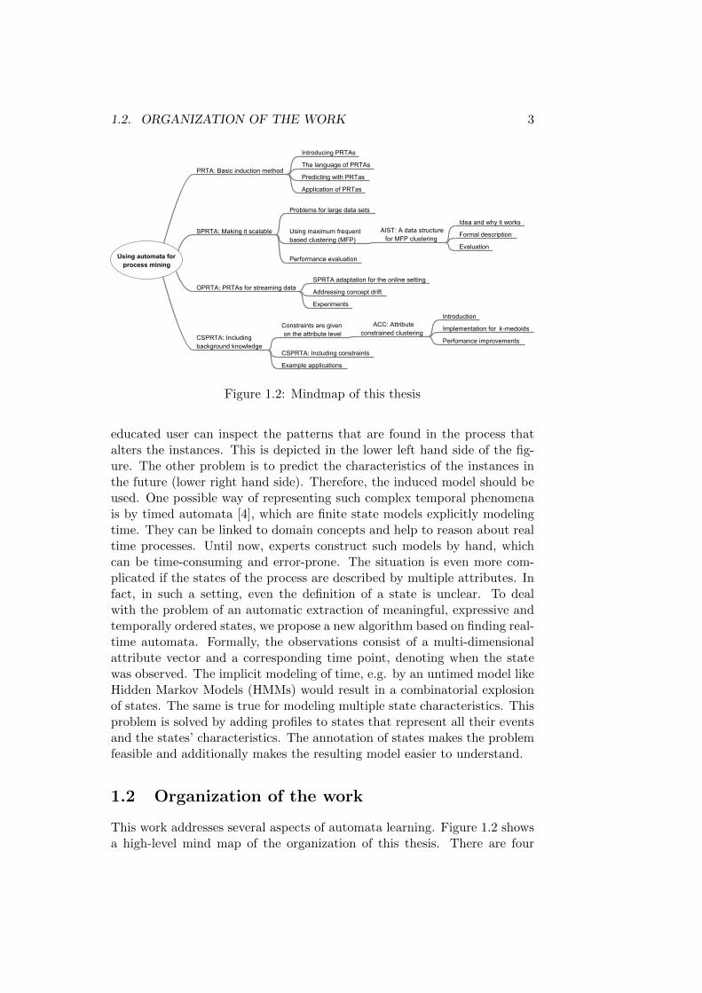
Figure 1.2: Mindmap of this thesis
educated user can inspect the patterns that are found in the process thatalters the instances. This is depicted in the lower left hand side of the fig-ure. The other problem is to predict the characteristics of the instances inthe future (lower right hand side). Therefore, the induced model should beused. One possible way of representing such complex temporal phenomenais by timed automata [4], which are finite state models explicitly modelingtime. They can be linked to domain concepts and help to reason about realtime processes. Until now, experts construct such models by hand, whichcan be time-consuming and error-prone. The situation is even more com-plicated if the states of the process are described by multiple attributes. Infact, in such a setting, even the definition of a state is unclear. To dealwith the problem of an automatic extraction of meaningful, expressive andtemporally ordered states, we propose a new algorithm based on finding real-time automata. Formally, the observations consist of a multi-dimensionalattribute vector and a corresponding time point, denoting when the statewas observed. The implicit modeling of time, e.g. by an untimed model likeHidden Markov Models (HMMs) would result in a combinatorial explosionof states. The same is true for modeling multiple state characteristics. Thisproblem is solved by adding profiles to states that represent all their eventsand the states’ characteristics. The annotation of states makes the problemfeasible and additionally makes the resulting model easier to understand.
1.2 Organization of the work
This work addresses several aspects of automata learning. Figure 1.2 showsa high-level mind map of the organization of this thesis. There are four

4 CHAPTER 1. INTRODUCTION
main projects: (1) the description of the basic model: probabilistic realtime automata (PRTA), (2) its adaptation to large, sparse data sets, (3) itsextension to data streams with concept drift and (4) the incorporation ofbackground knowledge.Chapter 2 reviews related work and puts this dissertation in the context ofautomata. As the described problem setting is closely related to graphicalcausal models, this chapter gives a short overview of the main approachesof this field. This includes Bayesian networks, Markov Random Fields andFactor Graphs. Although, these approaches model the dependency of spe-cific variables, a short explanation shows why they were not adopted in thiswork. Second, the domain of process mining that already addresses theinclusion of several instances in time will be discussed. Here, we focus onHidden Markov Models and Petri Nets as they are the most commonly usedmodels. Third, an extended overview of the domain of automata detectionwill be given. This also includes grammars and formal languages, but mainlyfocuses on the basis of this work: (timed) automata. Different induction al-gorithms are presented as well as applications. Finally, a summary reviewsthe necessary requirements for the algorithms that may tackle the problemsetting and indicates how this may be tackled.Chapter 3 summarizes all data sets that are used for the evaluation of thealgorithms, which include synthetic and real world data sets. Mostly, thesynthetic data sets are taken to address complexity and runtime issues, whilethe real world data sets (covering disease and gene expression data) showhow the resulting model can be interpreted. This helps to point out the ben-efits and shortcomings of the approaches. Additionally, we present qualitymeasures that enable the comparison of the different types of algorithms.This includes runtime, similarity to an original automaton and interpretabil-ity.Chapter 4 introduces the basic model: probabilistic real time automata(PRTA). The problem setting and the type of automata is formally defined.In the following chapter a description of how the basic function, the word-acceptance problem, of an automaton is solved. Section 4.1.2 describes theinduction algorithm of PRTAs and provides details about the used prefix treeacceptor (PTA), the underlying clustering, and the merge-function. The for-mal description of a PRTA concludes a presentation of how PRTAs can beused to predict future events. A subsequent experimental section evaluatesthe applicability of the proposed PRTA.Chapter 5 makes the PRTA scalable for large sparse data sets using anonline clustering algorithm. The approach is then referred to as scalablePRTA (SPRTA). An appropriate clustering method is discussed along withthe necessary mathematical functions. The basic idea is to find clustersthat share as many frequent patterns as possible. The patterns are found inthe instances that belong to a cluster. If large patterns are shared betweenthe instances, they are very similar and form distinguishable profiles of the

1.2. ORGANIZATION OF THE WORK 5
states. Experiments again show the applicability of this approach.Chapter 6 describes the basic data structure that is needed for the SPRTAalgorithm: the augmented itemset tree (AIST ). It is used to efficiently minemaximal frequent itemsets in an online setting, i.e. instances are observedone by one and each instance is only observed once. The AIST data struc-ture is evaluated under different points of view and its efficiency is analyzedfor various types of data sets. The main conclusion is that it is most appli-cable for sparse data sets consisting of large frequent patterns.Chapter 7 shows how background knowledge can be incorporated into theprocess of automata induction (constrained SPRTA CSPRTA). The ideabehind that is that for, e.g. medical data sets there are already some ex-pectations or even focus groups that a physician wants to explore. Suchexpectations can be easily described by using attribute constraints, i.e. con-straints that define the properties of the result. For example, consider anautomaton having a cluster with persons suffering from diabetes. Two dif-ferent types of constraints must-link and must-link-exclusive are defined andimplemented into the induction algorithm. Some experiments show whichtypes of constraints can be defined and used for this domain.The following Chapter 8 presents the basics for such a constrained inductionof automata. Here, the two constraints must-link and must-link-exclusive aredefined and evaluated in the k-medoids algorithm, which serves as a proofof concept. The constraints are then applied on synthetic and real-worlddata sets, which show how the performance of a clustering algorithm can beimproved if some background knowledge is taken into account.Chapter 9 presents the last extension of the PRTA, an approach that adaptsit to a genuine online setting (online PRTA OPRTA method). To do so, themain idea of the SPRTA-setting is adjusted to avoid the construction of thePTA. Additionally, the method is adjusted to include concept drift. Con-cept drift means that the underlying data generating process changes overtime. For the two examples, this may be the case when a new therapy isused that may cure a disease or its side effects, or if a new environmentalfactor stresses the cell so that other gene expression patterns are observed.In either case, this would change the underlying automaton structure so thatthe OPRTA-algorithm also has to adopt to such shifts.Chapter 10 summarizes the presented work, discusses the introduced algo-rithms and experiments and gives an outlook on future work.Finally, the contribution of this thesis can be summarized as follows:
• We present a new model to capture multivariate processes.
• We make this approach scalable and also provide an online inductionmethod.
• Therefore, we introduce a new algorithm for online maximum itemsetmining.

6 CHAPTER 1. INTRODUCTION
• Finally, we propose a new type of constraint to include backgroundknowledge for the proposed methods.
For each approach, a separate chapter formally defines the problem setting,the induction method and gives the results of the experiments on syntheticand real world data sets.

Chapter 2
Related Work
Today, temporal data are becoming available in many domains, where onlylittle is known about the processes generating the data. Example domainsinclude the internet (click paths), medicine (disease progressions) and bi-ology (life cycles of organisms, biochemical pathways). In this thesis, aprocess is assumed, described by states (or events) that are labeled with atime stamp and a multi-attribute vector holding M variables. The problemis to identify a model that fully represents the data and additionally forms ahypothesis about the underlying process. Additionally, it should be possibleto infer predictions. A potential solution to the problem comes from the fieldof graphical models. They give a compact representation of the processesand are easy to understand and interpret by the user. Although there existlearning algorithms for graphical models, they are often still created by anexpert (e.g. HMMs), which is unsuitable for an automatic and unbiasedmodel creation.The general task is to infer a probabilistic model, i.e. a model that providesa probability for the observation of a given instance, from data set S. Thedata set consists of several sequences: S = s1, . . . , sn, where a sequence con-sists of various symbols si = 〈si1, . . . , sik〉, sik ∈ Σ, and Σ is an alphabet.However, in the presented real world problems an element of Σ is not a singlesymbol but an attribute vector. Therefore, each of the presented approachesis also evaluated whether it is also capable of modeling a multivariate (time)sequence. A multivariate sequence si does not only consist of single symbolsbut of a sequence of feature vectors having m attributes sik = (a1, . . . , am).As a first step towards such complex time-series descriptions this work fo-cusses on binary feature vectors: al ∈ {0, 1}. Moreover, the multivariatesequences that are considered in this work are labeled with time stamps, i.e.si is a sequence of symbol-time pairs si = 〈(si1, t1), . . . , (sin, tn)〉.One problem that inspired this work is based in medical data mining: A pop-ulation of individuals is monitored over time. At individual-specific time-points, each person gives feedback about its health-status, which is a binary
7

8 CHAPTER 2. RELATED WORK
feature vector that indicates whether a specific disease is present. Usually,this monitoring is done at a physician who writes down all diseases that aperson suffers from. So, if a specific disease is not coded, the person is notconsidered to have it. Such visits may occur at different time steps, depend-ing on the person’s characteristics, so that the time intervals between the‘measurements’ may also vary. However, there will be a timepoint, wheresomeone wants to know in advance how this population will progress. Thiscould be a health care provider to plan capacities and utilization or healthcare sponsors for budget planning. Then, a forecast of the population’shealth status has to be done, using an adequate model. To show differentapproaches to this problem setting, graphical causal models and approachesfrom process mining with their benefits and shortcomings are presented.Subsequently, the approach of using automata is introduced and the currentlimitations are described in this section. Last, we give a short descriptionof how the benefits of all presented models could be combined into an au-tomaton.
2.1 Graphical causal models
Graphical models are used to model a complex system by describing thetopology of its components. That means that the dependencies of the com-ponents are described, i.e. which component influences another. A nextaim is to validate assumptions about the graph components and of courseto induce algorithms that make use of the topology in an efficient way. Be-sides, such a model should be translatable into a different form and moreover,should be understandable by other persons. In general, graphical models aredepicted by different types of entities: nodes and edges. Nodes representrandom variables (that may also be hidden) and edges reflect the dependen-cies between them. Hidden variables are a special type of the nodes and arefrequently used to model noise or unknown characteristics of the system.More formally, graphical causal models are (un)directed (acyclic) graphs ona set of random variables (RV). As these models should be as simple aspossible, RVs are grouped if they express similar dependencies. This makesit much easier for the user to identify which variables are independent fromanother under specific circumstances.To learn such a model from the training data one commonly expresses theconditional distributions or potentials as parameterized functions. By asmart choice of such a parameterized function, the computation of the modelparameters is much easier although the resulting type of model then is re-stricted. Usually a graphical model is constructed with prior knowledgeabout the model parameters. Each parameter that is known or believed tocontribute to the process behavior is included in the model. This is doneby considering each parameter as a random variable and then modeling the

2.1. GRAPHICAL CAUSAL MODELS 9
dependencies between these random variables. Each parameter can eitherbe an observable variables v = (v1, . . . , vT ) or a hidden variable (h(t)) withparameter θ, where T reflects the number of instances. Then, training datais used to find the best setting of parameters. The best setting is the onethat maximizes the probability of the training data:
P (h, v) = P (θ)T∏t=1
P (h(t), v(t)|θ)
This formalization can also be used in a time-related problem setting. Thenthe parameters can be considered as random variables at specific timepointsthat change over time:
P (θ(t)|θ(t−1))
There, the current value of a RV depends on the values of another set ofRVs. Using uniform priors often makes the computation of the remainingdependencies much easier by using only the likelihood. Conjugate priors alsooffer this advantage but moreover, allow for the inclusion of stronger priorknowledge. After having specified the parameters and variables of such asystem, algorithms are needed that calculate the specific values of the pa-rameters to find the best model. Often, correct algorithms are intractablein the computational costs and therefore, heuristics and approximations(like the expectation maximization algorithm) are applied. One applicationwhere such models are used is the detection of image segments [33] and genenetwork inference [19]. In the following, several different types of graph-ical networks will be presented. They all model the relationship betweenvariables in a (slightly) different way. After a short review of these meth-ods, each of them is examined whether it is possible to model time-series ofmultivariate event structures.
2.1.1 Causal networks
Causal networks (CNs) are a class of models that are based on directedacyclic graphs (DAGs) that model the dependency between variables. Inthe following, Bayesian networks, Markov Random Fields and Factor Graphsare described to illustrate how variables can be modeled. For all of thesetypes of models, one essential task is structure learning. Structure learningis necessary, if the true underlying causalities, i.e. which variable affects an-other, is not known. Of course, such a model should be as small as possiblebut should include all conditional dependencies of the given variables. TheIC-algorithm [68] achieves that by first identifying all pairs of independentvariables (a, b) for which an undirected graph is created that has an edgebetween a and b. Then a third variable c is tested whether it is dependenton the previous ones and if so, is added to the graph with v-like structure.Several additional constraints have to hold, and many improvements have
10 CHAPTER 2. RELATED WORK
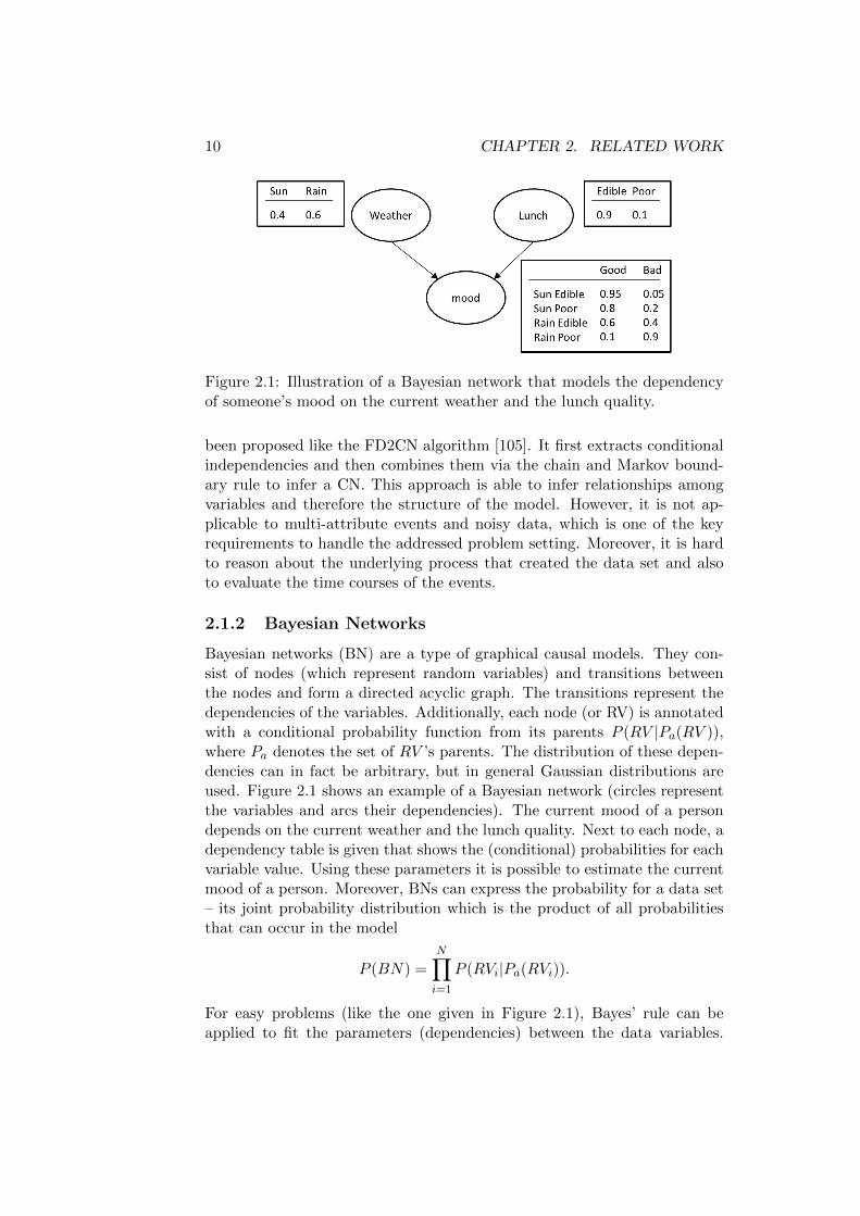
Figure 2.1: Illustration of a Bayesian network that models the dependencyof someone’s mood on the current weather and the lunch quality.
been proposed like the FD2CN algorithm [105]. It first extracts conditionalindependencies and then combines them via the chain and Markov bound-ary rule to infer a CN. This approach is able to infer relationships amongvariables and therefore the structure of the model. However, it is not ap-plicable to multi-attribute events and noisy data, which is one of the keyrequirements to handle the addressed problem setting. Moreover, it is hardto reason about the underlying process that created the data set and alsoto evaluate the time courses of the events.
2.1.2 Bayesian Networks
Bayesian networks (BN) are a type of graphical causal models. They con-sist of nodes (which represent random variables) and transitions betweenthe nodes and form a directed acyclic graph. The transitions represent thedependencies of the variables. Additionally, each node (or RV) is annotatedwith a conditional probability function from its parents P (RV |Pa(RV )),where Pa denotes the set of RV ’s parents. The distribution of these depen-dencies can in fact be arbitrary, but in general Gaussian distributions areused. Figure 2.1 shows an example of a Bayesian network (circles representthe variables and arcs their dependencies). The current mood of a persondepends on the current weather and the lunch quality. Next to each node, adependency table is given that shows the (conditional) probabilities for eachvariable value. Using these parameters it is possible to estimate the currentmood of a person. Moreover, BNs can express the probability for a data set– its joint probability distribution which is the product of all probabilitiesthat can occur in the model
P (BN) =N∏i=1
P (RVi|Pa(RVi)).
For easy problems (like the one given in Figure 2.1), Bayes’ rule can beapplied to fit the parameters (dependencies) between the data variables.

2.1. GRAPHICAL CAUSAL MODELS 11
However, in more complex systems this may lead to an intractable numberof variable combinations and thus to an enormeous runtime of the inferencealgorithm. To overcome such problems, one solution groups the variablesaccounting for their dependency relations and then exactly fits the parame-ters for this much smaller variable set. Second, an adequate splitting or eventhe elimation of variables can lead to more simple models. This can be ap-plied if some variable can be ruled out by background knowledge to have aneffect on the overall process. Third, approximations can be used to estimatethe parameters. Most commonly, maximum likelihood estimation is usedfor incomplete probability models. In contrast, a maximum-a-posteriori es-timation is used for complete BNs. To estimate the local maxima of thelikelihood (or a-posteriori) functions, standard optimzation algorithms likegradient descent algorithms are used. In the case that there are missingvalues in the data set, the EM-algorithm (expectation-maximization) canalso be applied to the induction of BNs. However, all these methods arebased on a given underlying RV-dependency structure. If this structure isnot known it has also to be inferred. Usually, this is then done in a greedyfashion. Elements (nodes and transitions) are added/deleted to the network,if a network specific score increases [34]. Then, this change is fixed in thenetwork structure. Such a score can for instance be related to the mini-mum description length (MDL) principle, which leads to the smallest modelproducing the least errors. BNs have been applied exentensively to modelcausal relationships. One example is the domain of genetic inference [19],where the interaction of genes shall be explored. However, BNs still modelsingle variables and have not yet been applied to modeling several discretevariables in parallel, i.e. the dependency of a set of variables is modeled inone node. Therefore, BNs remain unsuitable for the given problem setting.
2.1.3 Markov Random Fields
Markov Random Fields (MRF) also represent a set of random variables, butas a main difference from the previously introduced models, it is based onan undirected graph. Thus it may also be cyclic. There are three additionalproperties that make an undirected graph a MRF:
1. Any two non-adjacent variables are conditionally independent givenall other variables.
2. A variable is conditionally independent of all other variables given itsneighbours.
3. Any two subsets of variables are conditionally independent given aseparating subset.
The basic idea behind MRF is to model a set of variables, where the variablesare influenced by each ‘neighbours’. Moreover, there is an external ‘field’

12 CHAPTER 2. RELATED WORK
that also influences the behaviour of the variables [51]. This model was firstintroduced by Ising, a german physicist, who wanted to model magnetismof different metals. However, this idea could be very nicely applied to otherproblems, especially it could be transformed into a temporal relationship,because it can be shown that the Gibbs measure and the Markov chainmeasure are the same[51] under specific conditions. To apply MRF forother domains, it was applied on a graph, including its parameterization.Therefore, MRF that can be factorized according to cliques of the graph areused, because these probability distributions are much easier to establish.Along with the random variables a potential function (or clique potential)for each maximal clique is given gk(RVCk
), where Ck are the elements ofthe kth maximal clique. Of course, such an MRF can also model the jointdistribution. In this case, the joint distribution is expressed by the productof all potential functions divided by a normalization constant Z which givesthe partition function
P (MRF ) =1
Z
K∏k=1
gk(RVCk),
where
Z =∑
RV1,...,RVN
(
K∏k=1
gk(RVCk)).
Note that one essential difference to Bayesian networks is that in BNs theproduct of conditional probabilities is automatically normalized (Z = 1).Using the partition function Z for many concepts from statistical mechan-ics, such as entropy is very straight forward in MRFs because it gives anintuitive understanding of the process. Moreover, if one wants to examinethe effects of additional variables (like driving forces in statistical mechan-ics), i.e., how the system reacts on a pertubation, this is also done with theZ-function. To infer the conditional contribution the same estimation as forBNs can be done. Given one set of variables RV ′ for which the distributionhas to be inferred one takes another set RV ′′ and sums over all possibleassignments u /∈ RV ′, RV ′′. One application example for MRFs is the do-main of genome wide association studies [57]. The key idea is to include theeffect of linkage disequilibrium for single nucleotide polymorphisms (SNPs).A graph is created that holds an edge for each pair of SNPs that are consid-ered to be linked. If not, their occurence is considered independent. Then,a random binary variable is introduced for each SNP that shows whethera SNP is associated with a specific disease. Then, if SNP are in linkagedisequilibrium their values are encouraged to have the same values. Li et al.[57] applied this model to a neuroblastoma data set containing 1032 casesand 2043 controls. From approximately 32.000 genes 5 could be identifiedto have a high correlation with neuroblastoma and linkage disequilibrium.

2.1. GRAPHICAL CAUSAL MODELS 13
Figure 2.2: Illustration of the presented types of graphical models [60] forthe factorization p(u,w, x, y, z) = p(u)p(w)p(x|u,w)p(y|x)p(z|x).
2.1.4 Factor Graphs
Factor graphs (FG) subsume Bayesian Networks and Markov Random fields[33]. This also implies that BNs and MRFs can be translated into FGs.A FG is a bipartite graph for a set of RVs and a set of nodes that corre-spond to functions, where the product of all factors is the desired globalfunction, while the factorized functions (nodes) correspond to local func-tions. However, there is also an alternative presentation of factor graphsby Forney (Forney-style factor graphs [FFG ]) that use half-edges instead ofnode-functions. Figure 2.2 illustrates a FFG and moreover, shows how sucha FFG can be expressed as a MRF or a BN. Essentially, a factor graph canbe formed by applying the following rules [60]:
• There is a unique node for every factor.
• There is a unique (half-) edge for every variable.
• The node representing a factor g is connected with the edge (or halfedge) representing a variable x iff g is a function of x.
The joint probability is equal to that of MRFs. The expression of functionsby the nodes is very useful in the field of message passing algorithms (likebelief propagation) and has many applications in the field of coding or sig-nal processing like Kalman-filtering, which produces a model by stepwisemeasurements and parameter estimations.

14 CHAPTER 2. RELATED WORK
To sum up graphical models, one important fact is that they are a verypowerful tool to model variables and their dependencies. However, to thelarge number of variable combinations they may be inappropriate to modelthe influence of a set of variables on a set of other variables. Moreover, timeconstraints or a generalization of observations cannot be incorporated intosuch an approach.
2.2 Process Mining
Process mining tackles the identification of processes within a system withno external information. This also includes the identification of the elementsof the process and their temporal relation. For example, it may be unknownhow a process is actually conducted while another task may be to validatea predefined workflow. However, the main application is to find out theunderlying mechanisms of a specific process. Examples for such a problemare given by electronic medical records (EMRs1) that arise in hospitals orthe transaction logs of an enterprise resource planning system. Using suchlogs an analyst can identify the underlying sequences of frequently occurringtasks and derive optimizations or compare it to a predefined rule set to detecterrors or abnormalities.For the process induction of simple logs, of the shelve tools already exist2
that include a variety of algorithms, like Petri nets and Hidden MarkovModels (HMM). The tools can be applied to process logs consisting of simple,predefined events. They assume that it is possible to record events, i.e. theyneed a sequence of totally ordered events as input, which means that theevents occur one after another. Such event sequences are collected in so-called event logs, which then serve as data basis for the process miningalgorithms. Depending on the kind of process the user has to decide whichtype of model he expects. As one example, parallelism (when events canoccur in parallel) can only be detected by Petri nets, while switch or redo-tasks can also be modeled by HMMS. In contrast, Petri nets usually do notoffer probability distributions of the events/sequences that can occur or thefrequency of path-choices. In the following, two approaches – HMMs andPetri nets – for the induction of processes or sequence patterns are presented.
2.2.1 Hidden Markov Models
Hidden Markov Models (HMMs) are a special case of graphical models.Algorithms for graphical models were extended to first order HMMs (e.g.,for the MAP and inference problem [72]). First order HMMs consist of
1http://www.practicefusion.com/2http://www.promtools.org/prom6/

2.2. PROCESS MINING 15
hidden state variables (H) and observable variables (O), where the hiddenvariables define the underlying model. Hidden variables are connected bydirected edges. Each hidden variable has exactly one predecessor and anassociated observable variable, which is only dependent on the precedentvariables (Markov property). An HMM can be defined by a triple λ =(A,B, π). A is the matrix of state transition probabilities, B the observationsymbol probability and π the initial state distribution. Such a model isvery closely related to automata (cf. Section 2.3.2 as it can also provideestimations of the probability of sequences si (also denoted as words). Sucha probability can be calculated using HMMs by Equation (2.1) when the setof possible state sequences that may produce a word Q∗ is known.
P (si|λ) =∑v∈Q∗
P (si, v|λ) =∑v∈Q∗
P (si|v, λ)P (v|M) (2.1)
The fitting of the parameters of an HMMs (A,B, π) is achieved by maximumlikelihood estimation using the Forward-Backward algorithm [6] (also knownas the Baum-Welch algorithm) that converges to a local maximum. Giventhe observation sequence S and the model parameters λ, P (S|λ) is to bemaximized. This can also be viewed as choosing the hypothesis or model Aof all hypotheses A that maximizes P (S|λ) [30].
λMAP = arg maxλ∈L
P (λ|S) = arg maxλinL
P (S|λ)P (λ). (2.2)
Essentially this type of formulation arises from the Bayes framework thattries to optimize the tradeoff between the sample likelihood and the priorprobability. If all models are considered as equally likely then this frame-work chooses the model with the maximal likelihood, which is depicted inEquation
λML = arg maxλ
P (S|λ) = arg maxλ
m∏i=1
P (si|λ)P (λ). (2.3)
Interestingly, maximum aposteriori learning is the same as learning underthe minimum description length principle because Equation 2.2 can be re-formulated as
λMAP = arg minλ∈L
−log2P (S|λ)− log2(λ). (2.4)
Both terms show the encoding of the errors given the data set and the en-coding of the model.Although there exist quite a few solving schemes for the parameter fittingfor HMMs, the model learning task is a more complex problem. Addition-ally, there exist four further tasks: Evaluating, predicting, smoothing and

16 CHAPTER 2. RELATED WORK
decoding an HMM. Evaluation identifies the probability P (h|S, t) of a hid-den state h at a time point t dependent on an observed sequence S. Thiscan be calculated with the Forward algorithm. The second task, prediction,can also be solved by the Forward algorithm. Here, the probability P (h|S)of being in state h at time point t + δ (a time point in the future) is cal-culated, given t, δ and the emission sequence S. In contrast, smoothingcalculates the probability of being in state h at a earlier point in time t− δand is achieved by the Backward algorithm. The last task, decoding, calcu-lates the most likely hidden state sequence that produces a given emissionsequence S at the time point t. The Viterbi algorithm was devised for thistask. Both algorithms, the Baum-Welch and the Viterbi algorithm can alsobe applied in the domain of automata (when standard-sequences are mod-eled), especially in the case of probabilistic deterministic finite automata.There, the problem setting is even simpler as there exists only one path foreach word so that the computational complexity is reduced. In order tomodel time-labeled states of a process, where the states are described by amulti-dimensional attribute vector, a fully connected ergodic HMM couldbe used. Due to the fact that standard HMMs model only one-dimensionalvariables, there are two possibilities of what a state emits in this problemsetting. Either each state emits exactly one variable (symbol) or each stateholds a probability distribution over all variables O. Actually, the first caseis a special case of the second case, where each emission probability is setto zero except one, which is the one of the desired symbol.In the first mentioned model (one symbol per state), the structure of theHMM is defined as the set of all possible 2|O| states that are fully connected.Each state models one subset of variables. The resulting emission matrix Bis easy to determine: only one entry of the matrix is set to one, because eachstate emits exactly one of the 2|O| combinations of variables. The determi-nation of the transition matrix is computationally more expensive becausethere are |O|2 connections within the model. Therefore, A will be large andthere is no guarantee that each connection is represented in the data.The second HMM design for the given problem is to use only a certain num-ber of states which may emit all events. Here, all parameters have to beestimated from the data, especially the emission probability of each variablein each state. Thus A is quite small and B ≈ |M | ∗ |O|, but the numberof states has to be defined by an expert. If the designer follows inadequatehypotheses, the modeling will never be appropriate. However, in both casesthe complexity of the parameter estimation is mainly dependent on the num-ber of variables |O|. In the domain of multidimensional events, as it is thecase in our problem setting, the number of events (variables) is proportionalto the number of possible combinations of each variable dimension. Evenin the easiest case, where each event is described by d binary variables (soeach event is of dimensionality d), the number of possible states is equalto 2d. This quickly becomes infeasible with growing dimensionality [56] and

2.2. PROCESS MINING 17
makes multidimensional problems very hard for standard HMMs. To handlethe dimensionality problem, DT-HMMs [62] were proposed. However, theyare still not capable of modeling variables with more than two dimensions.So, other approaches to the two main drawbacks (multidimensionality andstructure learning) of HMMs were presented. To handle multi-dimensionalinput and output, Multi-Output HMMs [10] were proposed. However, totrain them, a hand-made structure has to be given a priori. For everyproblem, a hand-tweaked model is assumed, which strongly depends on theideas and intuitions of an expert. Nevertheless, there are tools like MoCaPy,which can be used to model Multi-Output HMMs and to fit models to givenobservation sequences. To learn the structure of HMMs, algorithms havebeen studied extensively, but rely on one-dimensional sequences [86] only.So, they are not appropriate for the problem setting that was outlined inSection 1.1 in their current form.
2.2.2 Dynamic Bayesian Nets
Dynamic Bayesian Nets (DBN) are a generalization of HMMs that use re-cursive HMMs to model time series. Here, several HMMs, possibly havingthe same structure, are combined via cross connections, so that each HMMmodels one time step [38] of a multivariate timed sequence. Such networksconsist of output nodes Yt, hidden states Ht and can optionally address in-put variables (Xt). The hidden states Ht in the DBN reflect multivariateattributes instead of a single random variable only (like it is the case forHMMs). Thus, the output variable Yt can also be multivariate. Althoughthis type of model can express very complex settings, the creation of such anet can be difficult. One aspect of the model is that one may have to knowupfront how many timesteps to include in the model. If, e.g., the model onlycaptures t timesteps, a prediction for the (t + 1)st timestep is not possible,because there was no training for this step. Moreover, the conditional de-pendency tables for such models may become very large, if Yt covers manydimensions: each possible combination of feature values must be estimatedfrom the training data, depending on the hidden states’ Ht variable setting(and the setting of Xt, respectively). Even for binary multi-dimensionalvariables, this may become intractable. Nevertheless, algorithms that learnthe structure of a DBN were proposed, like Bayesian model averaging [45]that estimates whether features (e.g., an edge in a graph) exist. Moreover,standard feature selection algorithms, such as forward or backwards step-wise selection for the identification of edges in such a model, or the leapsand bounds algorithm [42] can be applied, if the system is fully observable.

18 CHAPTER 2. RELATED WORK
Figure 2.3: Illustration of a Petri net.
2.2.3 Petri Nets
Petri nets [93] address the problem of identifying models from discrete eventlogs. These models can later be used to explain and transfer the acquiredknowledge. In general, Petri nets will only present the structural depen-dency, but will not give the joint probability P (si|λ) for an event sequencesi. Nevertheless, Petri nets can be used to learn log-based model structures.To describe Petri nets, there exist some variants, here Place/Transition net-works will be introduced, which are based on nodes and transitions. For-mally, a Petri net is a pair (N, s), where N is a tuple (P, T, F ) of places P ,transitions T (P∩T = ∅) and directed edges (flow relation) F ⊆ P×T∪T×P .The parameter s denotes the marking of the net. A marking is a bag overthe set of places P, i.e. it is a function from P to the natural numbersf : P → N that shows how many markers are given in the net. A node xcan be an input (or an output) node of another node y if there is an arcgoing from x to y (or vice versa). The set of all input nodes X of a node yis denoted as follows: •x = {y|(y, x) ∈ F}, and the set of all output nodesas x• = {y|(x, y) ∈ F}, for any x ∈ P ∪ T . The dynamics of Petri netsare given by firing rules that define when a transition is enabled: Transi-tion t ∈ T is enabled (indicated by (N, s)[t >), iff •t ≤ s. The firing rule[ > ⊆ N ×T ×N is the smallest relation for any (N = (P, T, F ), s) ∈ N 3
and any t ∈ T, (N, s)[t >⇒ (N, s)[t > (N, s − •t + t•). Figure 2.3 showsan example Petri net. Places are illustrated as circles while transitions aregiven by rectangles. There is also a token in this net, it resides in the sourceplace (the leftmost node), which is illustrated by the additional black circlein this node. In this example the source node is enabled and firing the tran-sition would move the token from the input place and puts it to the outputplace. As a result of this firing, place E and the AND-Split are enabled.Note that in a Petri net, tokens are consumed and produced, they do nottravers the net. This can be illustrated in the AND-Split: if this transitionfires then one token is consumed while there are two tokens produced. Asequence s is modeled (accepted) by a Petri net (N, s0), if there exists asequence of enabled transitions whose firing leads from s0 to s, given the
3N is the set of all marked, labeled Petri nets.

2.2. PROCESS MINING 19
Figure 2.4: Examples of a net (left) that cannot be detected by the α-algorithm, but a similar net is returned (right)
structure of the net and its markers [94]. There exist other characteristicsof Petri nets like connectedness, boundedness, safeness and liveness, whichwill not be described here. The structure of a Petri net is not only com-posed of places and transitions. As already shown in Figure 2.3, there arealso standard building blocks like AND-splits/joins or OR-splits/joins4 thatwere used to model the parallel, sequential or conditional processes. There,tasks are modeled by transitions while causal dependencies are modeled byplaces and arcs. Places can therefore also be considered as conditions thatmust take place before tasks. The structure of a Petri net is usually derivedby first finding an ordering relation of the events and then combining theminto an overall model. This does not include the frequency counts of thetransitions nor an automatic distinction of the events. All Petri net minersmust be given the set of events that may occur in an event log. Let’s considerthe α-algorithm as an example. First, the ordering of the events is extracted.This can simply be done by inspecting the ordering the events occur in thelog. If A always follows B than there can be established an sequential or-dering A→ B. Analogous, parallel orderings or even an unknown orderingcan be extracted. However, it is assumed that the log is always completeand that every possible relation between two events is observed at least onceif there is a relation. In contrast, it is not necessary to observe every firingsequence, because this may be impossible in a net with loops. Having thesecausal relations, places between them are created, which is the essentialproperty of many Petri net induction algorithms. However, places have tobe merged, if an OR-split/join is present. Moreover, short loops (of lengthone or two) are also a problem for the α-algorithm, which is also true forinvisible tasks. Figure 2.4 shows an example of a so-called non-free choicenet that cannot be identified by the α-algorithm. However, a similar netis returned instead. Although the α-algorithm cannot handle all types ofnet-types there exists work that has tackled some of the shortcomings of
4AND-constructs only have exactly one in (or outgoing) transition, while OR-constructsalways have multiple in and outgoing transitions
20 CHAPTER 2. RELATED WORK
the α-algorithm. The problem of short loops (α+ -algorithm) and implicitdependencies (α]-algorithm) was solved [28, 103]. To include invisible tasks,they are first separated into SIDE, SKIP, REDO and SWITCH constructsand then a new ordering relation that reflects the invisible tasks is intro-duced. The α++ -algorithm is also able to mine short loops by changingthe definition of log completeness (Loop-complete workflow log [28]) and byadapting the pre- and post-processing phases. There, the short loops areidentified in a last step that connects the short loops to the existing placesof the net.However, for more complex logs, e.g. numeric logs, the structure is fixed,while the parameters of the net are estimated [104, 52]. Although Petri netswere successfully applied to model business processes and biological path-ways, they are not applicable for the given problem setting (cf. Section 4).First, they are usually based on events that consist of one variable only andare therefore unable to model multi-dimensional events, and second, modelselection and capacity control remain essential open problems. While, onestraight forward way to handle multi-dimensional events would be to clusterthem first, and then to learn the net structure (cf. Section 4.2.7) a solutionfor the net constraints like, e.g. liveliness, was not elaborated, yet.
2.3 Automata
This section introduces grammars and languages together with their induc-tion algorithms and fields of application and discusses present methods forthe retrieval of automata.
2.3.1 Grammatical Inference
Grammars are very closely related to abstract automata and consist of rulesets that describe how words can be built up. Chomsky was the first scientistthat explored the properties of formal grammars. Nowadays, grammars arethe basis of important software components like compilers and are essentialfor the understanding of the capabilities of software and to verify all kindsof systems like communication protocolls. Especially for programs that arebuilt in a recursive structure. Consider the following example of a typicalrule: S → S + S. This expression means that a term can be created bycombining two other arbitrary terms by a ’plus’. Such a rule is very typicalfor the way, how software is implemented. Another important applicationfor grammars is to validate the structure of data, which is done by regularexpressions. They describe in a symbolic way how valid data must be setup.Such a problem can be handled by regular grammars. A grammar (or alanguage) L is defined over an alphabet Σ: L ⊆ Σ∗ and describes a final setof symbol sequences. Chomsky described a hierarchy of grammars, followingdifferent properties that can also be considered as automata. Figure 2.5
2.3. AUTOMATA 21
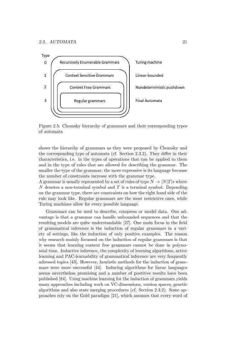
Figure 2.5: Chomsky hierarchy of grammars and their corresponding typesof automata
shows the hierarchy of grammars as they were proposed by Chomsky andthe corresponding type of automata (cf. Section 2.3.2). They differ in theircharacteristics, i.e. in the types of operations that can be applied to themand in the type of rules that are allowed for describing the grammar. Thesmaller the type of the grammar, the more expressive is its language becausethe number of constraints increase with the grammar type.A grammar is usually represented by a set of rules of type N → [N |T ]∗ whereN denotes a non-terminal symbol and T is a terminal symbol. Dependingon the grammar type, there are constraints on how the right hand side of therule may look like. Regular grammars are the most restrictive ones, whileTuring machines allow for every possible language.
Grammars can be used to describe, compress or model data. One ad-vantage is that a grammar can handle unbounded sequences and that theresulting models are quite understandable [27]. One main focus in the fieldof grammatical inference is the induction of regular grammars in a vari-ety of settings, like the induction of only positive examples. The reasonwhy research mainly focussed on the induction of regular grammars is thatit seems that learning context free grammars cannot be done in polyno-mial time. Inductive inference, the complexity of learning algorithms, activelearning and PAC-learnability of grammatical inference are very frequentlyadressed topics [43]. However, heuristic methods for the induction of gram-mars were more successful [44]. Inducing algorithms for linear languagesseems nevertheless promising and a number of postitive results have beenpublished [84]. Using machine learning for the induction of grammars yieldsmany approaches including work on VC-dimensions, version spaces, geneticalgorithms and also state merging procedures (cf. Section 2.3.2). Some ap-proaches rely on the Gold paradigm [21], which assumes that every word of

22 CHAPTER 2. RELATED WORK
the target language occurs at least once in the training data set S of stringsS ⊆ Σ∗. Using the provided examples one by one the learner constructsa model Ml that converges to the final solution. It stops when there isan example sn for which the induced target concept does not change anymore ∃n ∈ N : Mn = Mm, n < m. Usually, the following notation is used:Σ (and ∆) refer to non-empty finite alphabets. Σ∗ is equal to the set ofall strings over Σ and λ is the empty string (it is the only word havinglength 0 and is included in every language). A language L is a subset ofΣ∗ : L ⊆ Σ∗. Let u and w be two strings, u, v ∈ L, then their concatenationis illustrated by uv. A context (l, r) is an element of Σ∗ × Σ∗ which can bewrapped around a string: (l, r)� v = lvr. Languages can be concatenated:LM = {uv|u ∈ L, v ∈ M}. The set of all substrings of a word w (sub(w))can be defined as follows: {u | ∃l, r ∈ Σ∗, lur = w}. If applicable this is ex-tended to sets of strings. This notation is used to deduce whether a word ispart of a language. Depending on which deduction rule is applied, a partic-ular set of languages can be derived. This can be achieved by implementingrule schemas. For example, a schema could define whether a word can bededuced to be in a language by knowing that another word is in the lan-guage. By using a set of such rules [21] a language can be identfied. Chainrules are used to simplify the induction process. The link equivalence classesof rule sets then essentially describe the same languages. Rules can eitherbe correct, certain or defeasible. The first rules are always considered to becorrect, either by axioms or by the combination of information. However,if there is enough information to conclude that a rule is not correct thenit is considered as wrong. Still, the problem remains, whether an infinitelanguage contains a certain word. As such a word may be very long, it maybe impossible to conduct whether a rule is true or false. Therefore, eachrule is considered as defeasible until there is evidence that it is wrong. Todefine whether a specific word is part of the language L, proofs are derivedfrom the rules. Clark et al. [21] present a genetic algorithm that uses sucha rule system to find a grammar for a (in general unbound) set of examplesby retrieving information from a so-called oracle that defines whether or notan string is part of the language so far. This is similar to the famous L*algorithm by Angluin [9] (cf. Section 2.3.2). Using this type of notationand proof formalism many types of languages can be inferred, e.g. MultipleContext-Free grammars or even linear grammars.There also exists an extension to stochastic grammars, where a probabilitydensity function over Σ∗ ist given, i.e. there is a probability for each wordw ∈ Σ∗ to occur in the language L. The stochastic grammars that formsuch a stochastic language need and additional factor: a probability thatthe grammar L creates the string/word w which is defined recursively:
p(X ⇒ λ) = p(X → λ)
p(X ⇒ aw) = p(X → aY )p(X ⇒ w)

2.3. AUTOMATA 23
To find such a grammar the RLIPs -algorithms was introduced that findsthe equivalent automaton (cf. Section 2.3.2). It was applied to speech recog-nition with noise or other random errors. Another application for stochasticgrammars is the identification of structural elements by markups in textdocuments [106]. One nice property of this approach is that the grammarevolves as new examples arrive and thus a better interactive tuning of theresult is possible.
2.3.2 Automata Induction
The term automata was introduced in the 1930s by Alan Turing, who studiedwhich problems can be computed and which not. This is also formalized bythe term determinable that includes all problems that can be solved withcomputers. The second questions is, which problems can be managed bycomputers, i.e. can be solved within a time span that grows slowly withthe size of input. Slowly means that the time can be approximated by apolynomial function. However, this work will not discuss such problems butaims at describing how automata can be used to formally describe processesor systems. In general automata can be considered as a system that consistsof a set of states that describe some important properties of the system.Moreover, the system is described in a way that it is exactly in one stateat each time point. As there is no memory, former states of the system are‘forgotten’ when a new state is reached. Given an input sequence, which maybe any symbol of an alphabet, the automaton changes its state according tothe provided symbols. Note that there exist only a specific set of start states,i.e. states which ‘accept’ the first symbol. Final (Accepting) states describewhether the system is in a valid state. If such a state is reached after aninput sequence, the sequence is considered as valid. Figure 2.6 shows a very
Figure 2.6: Example automaton
simple example automaton that consists of five states. If this automatonreceives as input the letters t−h− e−n it reaches the only accepting state.Thus, this automaton is built to parse (or to identifiy) the word then.
Types of Automata To describe the class of automata more formally,let’s consider one main distinction of automata first: determinism. Anautomaton is deterministic if it can reside in exactly one state at eachpoint in time. Formally a deterministic finite automaton (DFA) is a tu-ple Γ = (Q,Σ, δ, q0, F ), where

24 CHAPTER 2. RELATED WORK
(a) Example DFA
(b) Example NFA
Figure 2.7: Top: Example of a DFA. Bottom: Example NFA. Both automataaccept the language of words that end with 01
• Q is a final set of states
• Σ is a final alphabet
• δ is a transition function δ : Q,Σ → Q) that defines for each stateq ∈ Q and symbol a ∈ Σ the next state q′ ∈ Q
• q0 is the start state q0 ∈ Q
• F is the set of final states F ⊆ Q
A DFA can decide, whether a word (sequence of symbols) is part of a lan-guage – whether the word is accepted. If a langugae, i.e. a set of words isa accepted by a DFA, this language is called regular language (cf. Figure2.5). Nondeterministic finit automata (NFA), i.e. automata that can residein several states simultaneously, also accept regular grammars, but are of-ten easier to describe. This can be proven by the fact that each NFA canbe transformed in a DFA. Such a type of automaton can be in two statessimultaneously because there may be states that have several alternativeswhen a specific symbol is read. That means that there is more than onenext state. Figure 2.7b shows an example for such an automaton. The dif-ference to a DFA is that there are states for which there is no next statefor some symbol σ ∈ Σ. Thus, the definition of such an automaton dif-fers only in function δ : Q,Σ → Q∗. One important subclass of automataof DFAs are distinguishable automata. This property is fullfilled if thereare no two states s and s′ and their corresponding trajectories Ps and Ps′ ,where the two trajectories are too similar concerning one similarity metricm: m(Ps, Ps′) ≥ µ,∀s, s′ ∈ Q.

2.3. AUTOMATA 25
Probabilistic automata (PA) were developed to model probabilistic sys-tems [87] and subsume Markov chains and Markov decision processes aswell. Given an NFA a PA can be constructed with it by adding a probabil-ity distribution to each state’s transitions that define the probability p(qi, a)that symbol a is observed after state qi. As usual the sum of probabilitiesof the transitions leaving each state sum up to one.
Learning Automata As described before, automata, grammars and graph-ical causal models (like HMMs) are very closely related and can be used forsimilar problems. Due to their intuitive structure HMMs were the initialchoice for modeling time series in many domains. However, for their correctparameter induction (usually the EM-algorithm is used), which is indeedonly locally optimal, the correct underlying topology must be known. Thisis not necessary when inducing automata [36]. Note that in general eachHMM can be transformed in (or at least approximated by) an equivalentautomaton (having the same number of states) and vice versa (while herethe HMM has not necessarily the same number of states) [36]. When in-ducing the structure of automata, there exist three main streams in theliterature, using the state merging method [12], algorithms that guaranteePAC-learnability [22] (more generally probabilistic models) and a set of algo-rithms similar to the L∗ algorithm [9]. The aim when learning probabilisticautomata is the induction of a distribution from a sample that is as similaras possible to the (unknown) target distribution. In the easiest case someprior knowledge is given to the learner so that the topology of the modelcan be fixed before the parameter estimation. If this is not possible, thenstructure learning and topology modeling has to be done together [30]. Suchapproaches have already been shortly introduced in Section 2.2.1 and canalso be adopted for specific classes of automata as HMMs can be transformedinto automata (PDFAs).The second main type of the induction of automata is derived from the L∗
algortihm, which learns a minimal DFA for a given regular language. Themain idea behind such methods is that there exists a learner that has to pro-vide the final automaton. The learner may ask questions to a teacher whoknows the correct automaton as well as a so-called oracle that can decidedwhether the proposed automaton is correct. This setting is schematicallyillustrated in Figure 2.8. The L∗ algorithm is based on two sets U ⊆ Σ∗
(words that are candidates for identifying states) and V ⊆ Σ∗ (words todistinguish states). The learner identifies candidate words from (U ∪UΣ)Vand queries the teacher whether they are part of the language. The resultof this query is stored in a table T = (T ,U ,V). The learner tries to identifya closed and consistent language H from this table and queries the oraclewhether this is correct. If the automaton is not correct, the oracle returns acounterexample that is used to update the sets U and V accordingly. This

26 CHAPTER 2. RELATED WORK
Figure 2.8: Illustration of the problem setting for by the L∗ algorithm [9]
leads to the creation of new membership queries until the language is againclosed and consistent. This is repeated until the correct language is identi-fied.Although there exists much theoretic work about the bounds and quality ap-proximations using such algorithms, the third induction group (state merg-ing methods) has proven well in practice. They require a significant smallersample size to infer the given automataon (or grammar) [14]. Automatainduction methods that rely on the state merging strategy are based on aso called prefix tree acceptor [30], which is a DFA that can only generatethe data set S, i.e. no generalization is present. Upon such a structure themerging procedure is applied. Nodes of the PTA are merged (combined intoone state) successively. The search space of such a method is given by allautomata that can be derived by merging the states of a PTA, from whichthe best fitting model has to be selected. How ‘best’ is considered will be de-scribed in the following sections and is different in the specific approaches.Nevertheless, Algorithm 1 shows a generic learning scheme for inductionmethods relying on the state merging procedure. It uses the given dataset S and a precision parameter that is dependent on the specific merge-criterion. The basic steps are first, the selection of pairs of nodes that areconsidered for merging (SelectStates), then the evaluation whether they arecompatible (which is also depending on the specific algorithm) and if so theupdate of the current automaton. The update is essentially the merging ofq and q′. The following algorithms can be considered as specifications of oneof these main steps each. One example of algorithms that implements thisbasic structure is the Alergia algorithm [12]. The sequences are selectedin alphabetical order and evaluated in pairs whether to be merged. This isthe case when the following condition, derived by the Hoeffding bound, isfullfilled:
∀a ∈ Σ :

2.3. AUTOMATA 27
Algorithm 1 General state merging method (Histories H, precicion param.µ)
1: Γ← PTA2: while stopping criterion not satisfied do3: (q, q′)← SelectStates(Γ)4: if Compatible(q,q’,µ) then5: Γ← Update(Γ, q, q′)6: end if7: end while8: return Γ
∣∣∣∣C(q, a)
C(q)− C(q′, a)
C(q)
∣∣∣∣ <√1
2ln
2
µ
(1√C(q)
+1√C(q′)
).
This condition compares the outgoing transitions of state q and state q′ re-spectively and also recursively the successore states of q and q′. If q andq′ are compatible, they – as well as their successors, if appropriate – aremerged to eliminate non-determinism. This strategy is therefore called de-terminization by merging. This algorithm identifies the class of probabilisticdetermininistic regular languages in the limit.The basic algorithm was also modified to induce acyclic automata [73] re-flecting finite languages. There, candidate states must be in the same depthof the PTA to be merged to ensure the acyclicity. Besides, states must befrequent to be merged. Otherwise they are combined into one state thatreflects exceptions. Finally the transition probabilities are corrected by themaximum likelihood estimates:
ϕ(q, a) =C(q, a)
C(q)(1− (|Σ|+ 1)ϕmin) + ϕmin
, where ϕmin is the minimal transition probability in the automaton. An-other adaptation is the MDI algorithm [88] that aims at finding of minimalsizes and small deviations from the data set S. Here again the two states qand q′ are merged to a temporary solution Γ1 and eventually with additionalstates to solution Γ2. This is done if the divergence increment relative tothe new (smaller) size of the automaton is less then µ:
D(Γ0||Γ2)−D(Γ0||Γ1)
|Γ1| − |Γ|< µ,
where D(Γ0||Γ2) reflects the divergence of the automata Γ1 and Γ2.The RLIPs- algorithm [13] also uses the state merging method on a prefixtree acceptor to find the minimal stochastic automaton for a given stochas-tic regular language from a positive data set only. Therefore, a branchand bound algorithm is used. This type of algorithm is also able to identify

28 CHAPTER 2. RELATED WORK
cyclic structures of an automaton and was proven to converge having a lowerbound on the provided data set. In 2006, Gavalda et al. proposed a frame-work (based on an algorithm of Clard and Thollard [22]) that is based ona state merging and splitting strategy [36]. The induction strategy of suchalgorithms is incremental although the necessary statistics are computed ina batch mode. Starting from an automaton that includes all knowledge thatcould be collected up to this timepoint, a new sequence is mapped againstthe automaton until its end is reached or one symbol of the sequence reachesa so called candidate node u. This is the case when there exists no transitionlabeled with σi out of the current (safe) node w. If there is no safe node vsuch that u is similar to v (which is tested every time after reaching u) thenu is promoted a safe node and added to the list of final states of the au-tomaton. This can be summarized as described in Algorithm 2. Moreover,
Algorithm 2 CT Algorithm (Trajectories D) [36]
1: for all d ∈ σ0, . . . , σk do2: while σi matches a state s do3: a safe state can be reached4: i++5: end while6: if i < k then7: candidate state s is reached8: if s is not large/frequent then9: retain node s
10: else if s has a similar state s′ then11: merge node s with s′
12: else13: promote s a new safe state14: end if15: else16: add σi+1, . . . , σk to Dsσi
17: end if18: end for
this algorithm ensures that
For every PDFA M with n states, with distinguishability µ > 0, such thatthe expected length of the string generated form every state is less than L ,for any δ > 0 and ε > 0 , the PDFA-Learn algorithm will output a hypoth-esis PDFA M’ such that, with probability greater than 1 − δ, the maximumdifference in the probability assigned by the PDFA to any string is at mostε .[36]
However, the algorithms proposed by Castro et al. [14] differs in one main
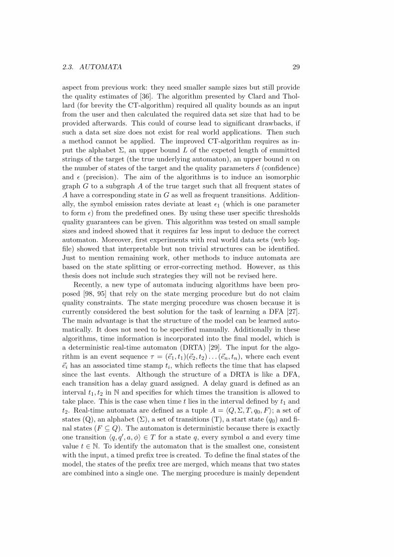
2.3. AUTOMATA 29
aspect from previous work: they need smaller sample sizes but still providethe quality estimates of [36]. The algorithm presented by Clard and Thol-lard (for brevity the CT-algorithm) required all quality bounds as an inputfrom the user and then calculated the required data set size that had to beprovided afterwards. This could of course lead to significant drawbacks, ifsuch a data set size does not exist for real world applications. Then sucha method cannot be applied. The improved CT-algorithm requires as in-put the alphabet Σ, an upper bound L of the expeted length of emmittedstrings of the target (the true underlying automaton), an upper bound n onthe number of states of the target and the quality parameters δ (confidence)and ε (precision). The aim of the algorithms is to induce an isomorphicgraph G to a subgraph A of the true target such that all frequent states ofA have a corresponding state in G as well as frequent transitions. Addition-ally, the symbol emission rates deviate at least ε1 (which is one parameterto form ε) from the predefined ones. By using these user specific thresholdsquality guarantees can be given. This algorithm was tested on small samplesizes and indeed showed that it requires far less input to deduce the correctautomaton. Moreover, first experiments with real world data sets (web log-file) showed that interpretable but non trivial structures can be identified.Just to mention remaining work, other methods to induce automata arebased on the state splitting or error-correcting method. However, as thisthesis does not include such strategies they will not be revised here.
Recently, a new type of automata inducing algorithms have been pro-posed [98, 95] that rely on the state merging procedure but do not claimquality constraints. The state merging procedure was chosen because it iscurrently considered the best solution for the task of learning a DFA [27].The main advantage is that the structure of the model can be learned auto-matically. It does not need to be specified manually. Additionally in thesealgorithms, time information is incorporated into the final model, which isa deterministic real-time automaton (DRTA) [29]. The input for the algo-rithm is an event sequence τ = (~e1, t1)(~e2, t2) . . . (~en, tn), where each event~ei has an associated time stamp ti, which reflects the time that has elapsedsince the last events. Although the structure of a DRTA is like a DFA,each transition has a delay guard assigned. A delay guard is defined as aninterval t1, t2 in N and specifies for which times the transition is allowed totake place. This is the case when time t lies in the interval defined by t1 andt2. Real-time automata are defined as a tuple A = 〈Q,Σ, T, q0, F 〉; a set ofstates (Q), an alphabet (Σ), a set of transitions (T), a start state (q0) and fi-nal states (F ⊆ Q). The automaton is deterministic because there is exactlyone transition 〈q, q′, a, φ〉 ∈ T for a state q, every symbol a and every timevalue t ∈ N. To identify the automaton that is the smallest one, consistentwith the input, a timed prefix tree is created. To define the final states of themodel, the states of the prefix tree are merged, which means that two statesare combined into a single one. The merging procedure is mainly dependent

30 CHAPTER 2. RELATED WORK
on the final structure of the automaton. Automata not including a delayguard may use (k, h)-contextuality [3] to identify the states to be merged.Here, similar paths are identified and then k − h + 1 states of the pathsare merged. However, for automata with delay guards, the deterministicconstraint can be violated after a merge: There may be two transitions withthe same symbol and delay guard. This mismatch is resolved by a splittingprocedure that creates two paths in the prefix tree with non-intersectingdelay guards. Although state merging is currently state of the art, thereexist different methods of how to merge and split states and transitions.One possibility is to do splits and merges depending on their consistency(derived by a χ2 test [96]) and apply a rule set to identify whether a mergeor a split is the best next step. Note that this algorithm relies on positivedata only, which means that all input data are expected to be part of thelanguage that is formed by the automaton and thus must be accepted by it.Another method to find the best split or merge is to compute the likelihoodof an overlap of the two tails of a state in the prefix tree [99]. Again, a scoreis computed to select the best operation (merge or split). This operation isbased on the red blue algorithm.Still, one has to remark that automata and causal models are closely re-lated. Comparing, e.g. automata to HMMs, the parameter λ of the au-tomaton is again a transition matrix B, which is derived by ML estimation(parameter learning problem). It covers transition probabilities dependingon multi-dimensional symbols and time: bij = P (transitionij |~ek, tk). Theintroduction of probabilities offers the possibility to construct a generative(automaton based) model and to compute the probability P (S|λ) for eachobservation sequence S depending on the model parameter λ. Moreover,prediction (although in general not important for automata) is also a de-sired function in this work and will be discussed in depth in Section 4.1.3. Incontrast, the evaluation task has no true equivalent in the world of automata.The same is true for smoothing and decoding. In general, it is not importantto know in which state an automaton resides but if the automaton acceptsthe sequence S. This shows whether a sequence S is part of the languagethat is modeled by the given automaton. Moreover, deterministic automataprovide no transition probabilities, so the calculation of state sequences isstraightforward. Considering non-deterministic probabilistic automata, itis possible to compute P (h|S) depending on the transition probabilities, sothat smoothing, decoding and evaluation can in principle be conducted as inthe domain of HMMs. However, as stated above, answering these questionsis not the main task of automata. It is only of interest whether a sequenceS is accepted by an automaton.

2.4. APPLICABILITY TO THE PROBLEM SETTING 31
2.4 Applicability to the problem setting
The main idea of this work, was to enable the temporal analysis of biologicaland medical data sets. The important subdomains here are first the pre-diction of disease progressions in a population (cf. Chapter 2) and secondthe identification of relationships between genes. One task is to find out inwhich sequence a cell expresses which genes. Another task is to find outhow the genes interact with each other and the resulting metabolic state ofthe cell. This also includes the transduction of signals within a cell, which isvery complex and by no means already understood. Nowadays, microarrayexperiments allow for the simultaneous evaluation of several thousands ofgenes over a specific time period under various environmental constraints.Then, the genetic interactions and cell-responses to stress can be observed.Therefore, the information of how genes interact and depend on each otheris very interesting and there are quite a lot of approaches to deal with suchproblems. One possibility is the extraction of temporal association rules(TARM)[65]. However, most of the approaches suffer from the problem thatthere exist very many genes but only a few timepoints of observations. Thus,using analytical/Bayesian approaches (covariance analyses and so forth) maynot result in appropriate results as the number of training instances is verysmall and there may be too few observations for an approximately correctestimation. Besides, the incorporation of time constraints is also one essen-tial point. The user wants to specify which time periods has to be modeled,i.e., how the gene expression ratios develope after, e.g. 10 minutes. Thenext issue is that the events or characteristics are not necessarily knownupfront, so that the desired algorithm must find out states or appropriatevariable settings without prior knowledge. One obstacle here is that theremay be noise, which blurs events and lets them seem different although theyare actually the same. One example here is that a genetic experiment in-correctly returns a negative expression for a gene because it was just notsensitive enough. Therefore, we define a list of characteristics that have tobe covered by an approach to produce an understandable model that canhandle the discussed problems. The model should
• produce a probabilistic generative graphical model,
• handle multi-dimensional variables,
• consider time stamps,
• allow for cycles, and
• generalize similar events due to noise.
Up to now, all the discussed approaches can deal with one or more of thedesired properties, but all of them have limitations that are not easy to

32 CHAPTER 2. RELATED WORK
solve. However, automata have already been extended to take into accountthe time constraint. Therefore, we decided to push this extension forwardand to create an automaton-based model that not only automatically definesits states from the given set of events, but also may address noise and cyclicstructures.
2.4.1 Combining the best of the presented approaches
All existing automaton based algorithms are made for one-dimensional eventsonly. Nevertheless, only few modifications are required to deal with multi-attribute events. To do so, an approach to combine probabilities with au-tomata was presented [96]. It models one-dimensional symbols and timeby using interdependent probability distributions, but transition intervalsmust be given in advance, which leads to a model with many parameters.In contrast, we solve the problem of multi-dimensional attributes by an-notating states with dynamic profiles instead of symbols, and derive jointprobabilities for transitions during the merge operation. In this way, selectedproperties of HMMs (transition probabilities, Markov property), causal net-works (graphical representation), Petri nets (cyclicity) and automata (delayguards) are combined with a generalization approach, to obtain the desiredfunctionality. Definition and inference of such an automaton will be pre-sented in Chapter 4 and its subsequent extensions for large sparse data sets(Chapter 5) and to incoporate background knowledge (Chapter 7). Last,an approach to handle data streams, even with concept drift is presented(Chapter 9). These algorithms and their results are summarized and, fur-ther, interesting work, like an algorithm improvement for dense data sets,will be introduced.
Chapter 3
Preliminaries: Materials andQuality Measures
3.1 Data
In this section we briefly introduce the synthetic and real world data sets weused for the evaluation of the algorithms. Synthetic data are used to evaluatethe correctness of the method and real-world data are used to examine thedescriptive power. The real-world datasets encompass medical and biologicaldata. Data sets that were used exclusively for the evaluation of specific partsof the PRTA induction are described separately in the specific chapters.
3.1.1 Synthetic data
A first benchmark is always whether the proposed algorithm can reproducea predefined structure, i.e. an automaton, like it was done in existing work[36]. To show that the algorithm rediscovers an automaton that is known,histories were produced by a synthetic automaton (cf. Section 4.1 for thenomenclature of used automata). To do so, we created an automaton with10 states and 10 attributes. This automaton produced 100 synthetic his-tories by traversing the states corresponding to the transition probabilities.For each history the profiles of the visited states were saved. Afterwards,those histories were used as input for the algorithm. Additionally, with anerror ratio of 0.1, we randomly generated errors in the profiles to see if theautomaton will be detected correctly although the states are not completelyequal. With a probability of 0.1, each attribute of a profile is changed intoits opposite. If it is one, it will be changed to zero, and vice versa. Thegoal of the introduction of errors is to test if the algorithm will neverthelessproduce the correct structure although noise is present. The handling oferrors is important because real-world data is expected to be error-prone.Figure 3.1 shows the synthetic automaton that produced the synthetic his-
33

34 CHAPTER 3. PRELIMINARIES
Figure 3.1: Illustration of the synthetic automaton used in the experiments.Each circle is a state, each arrow a transition. The actual profile of each stateis given in brackets and each transition is labeled with its probability. Forsimplicity, the delay guard (not illustrated) on each transition is φ = [1, 1].
tories. Transitions are labeled with probabilities, and next to the states allattributes that are equal to one are shown (in brackets). They correspondthe profiles. Delay guards are always equal to one and can therefore beneglected in this case. The described automaton was also used for a proofof concept and further stability analyses (cf. Section 4.2). Therefore, a dataset containing 100 histories of average length 10 was produced by traversingthe automaton corresponding to the transition probabilities. For a stabil-ity analysis (cf. Section 5.2), ten more synthetic data sets were created inthe same manner. They serve as a starting point for a bootstrap analysis.From each of these ten data sets, 100 derived data sets are created by thebootstrap method. Thus, 1000 data sets are used in the stability analyses.To examine the algorithm’s scalability for data streams, even larger datasets were created (cf. Section 9.2). They range from 50 to 100,000 histories,where the history length was fixed to be 100. Again, to account for dataset variability, for each number of histories 10 data sets are created. Toaddress the stability of the algorithms when noisier data sets are present,the synthetic automaton was also used to create data sets having a differ-ent amount of noise. This error ratio ranges from 0.1% to 10%. Anotheranalysis addresses the algorithms dependency on the length of the histories.Thus, the synthetic automaton also served as a basis for data sets havingdifferent history lengths. They were varied between 10 an 1000, while the

3.1. DATA 35
data set size was fixed to 10,000.
3.1.2 Real World Data Sets
Disease Group Data Set I
The first real-world, proprietary dataset comprises diagnosis data from 1000persons from four years. Each diagnosis was grouped into one of 106 medi-cally motivated disease groups (DGs) and saved with its timepoint, namelythe year it occurred in. The grouping is based on the similarity of dis-ease patterns and the probable progression, relying on the three-digit WHOICD101 codes of chronic conditions. For each timepoint, we obtain 106 at-tributes that represent the event of the timepoint (cf. section 4.1). However,the attributes of events are quite sparse: Just 28 out of 106 DGs occur inmore than 5% of the instances, 66% of all events just have one or two DGsset, and 99% of the events incorporate less than 11 DGs. Thus, only DGsthat occur often (in more than 5% of the instances) were used to defineevents. Because this data set shows the progression of diseases, only in-stances having at least one timepoint with an event e where |~e| > 0 wereincorporated into the histories.
Disease Group Data Set II
The last (non-public) data set covers historic diagnoses from 147’656 pa-tients within four years on a quarterly basis2. Thus, this data set showsthe progression of diseases within a population. As there are about 15’000diagnoses (ICD codes), each provided diagnosis was grouped into one of 111clinically homogeneous diagnosis groups that combine several diagnoses cor-responding to their similarity and expected outcome. Using this compressedmedical representation enables the user to manually inspect and judge theresulting states of the automaton. Therefore, a history is a feature vector fora patient and timepoint t describing the set of disease groups at timepointt. We used two derived data sets to build the automaton. The first dataset only contains disease groups (DGs) that occurred in at least 10% of allpatients (22 attributes) in order to obtain the most frequent and importantdisease patterns (P10). The second data sets includes all disease groupsthat occurred in at least 1% of all patients to allow for a more extended in-spection (76 attributes, P01). The final PRTA then shows which diseases anspecific population suffers from and which transitions between such diseasestates occur and how often. This may enable physicians to better foreseefuture impairments.
1http://apps.who.int/classifications/apps/icd/icd10online/2We gratefully acknowledge Gesundheitsforen Leipzig GmbH

36 CHAPTER 3. PRELIMINARIES
Figure 3.2: Illustration of the binary yeast cell cycle data, the rows representfeatures, columns instances/different timepoints. If an attribute is equal toone, it is represented by the corresponding (colored) number.
Hepatitis Data Set
The next data set is the 2004 ECMLPKDD Hepatitis challenge data set3. Itcontains blood test results for 1236 patients suffering from either HepatitisB or C between 1982 and 2001. Next to some demographic informationlike age and sex, the results of up to 36 tests are given for each individualexamination. Some patients are only recorded once while others have ahistory of 401 records. However, 95.7% of the patients provide a history ofat least two events, where one event is considered as the examination resultof one day. The fillgrade of the attributes in this data set varies strongly.To obtain meaningful results, only the attributes that are present in at least80% of the events were included in the histories. Moreover, each attributewas discretized in three subtypes: blood test result below normal, normaland above normal. For missing test results none of the attribute’s valueswas set. Thus, the final events consist of 33 attributes (cf. Table 7.2 for ashort overview). To evaluate the algorithm’s scalability, several data sets ofdifferent sizes (50, 100, 150, 200, 300, . . ., 900, 1000, 1236 histories) werecreated.
Yeast metabolism data
A further real-world data set holds the gene expression values of buddingyeast [74] (GEO ID: GSE3431) that were recorded using Affymetrix chips(GPL90) for 36 timepoints with a delay of 25 minutes each. The data setcovers the expression rates of 9335 genes of a synchronized (all cells start inthe same state) cell culture and is freely available4. As cells also change intheir metabolism, genes are expressed (used) at different time steps, reveal-ing expression peaks in the data. These peaks give information about thecurrent state of the cell, e.g. which metabolism is currently activated. How-ever, the data is given as an expression series of continuous variables andnot as zero/one vectors (gene is off/on). Therefore, the expression profiles
3http://lisp.vse.cz/challenge/ecmlpkdd2004/4ftp://ftp.ncbi.nih.gov/pub/geo/DATA/SeriesMatrix/GSE3431/
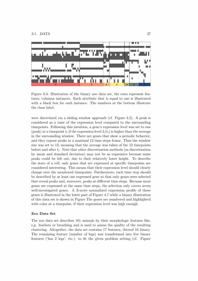
3.1. DATA 37
Figure 3.3: Illustration of the binary zoo data set, the rows represent fea-tures, columns instances. Each attribute that is equal to one is illustratedwith a black box for each instance. The numbers at the bottom illustratethe class label.
were discretized via a sliding window approach (cf. Figure 3.2). A peak isconsidered as a raise of the expression level compared to the surroundingtimepoints. Following this intuition, a gene’s expression level was set to one(peak) at a timepoint ti if the expression level L(ti) is higher than the averagein the surrounding window. There are genes that show a periodic behavior,and they expose peaks in a maximal 12 time steps frame. Thus the windowsize was set to 12, meaning that the average was taken of the 12 timepointsbefore and after ti. Note that other discretization methods (as discretizationby mean and standard deviation) may not be as expressive because somepeaks could be left out, due to their relatively lower height. To describethe state of a cell, only genes that are expressed at specific timepoints areconsidered interesting. This means that their expression level should clearlychange over the monitored timepoints. Furthermore, each time step shouldbe described by at least one expressed gene so that only genes were selectedthat reveal peaks and, moreover, peaks at different time steps. Because mostgenes are expressed at the same time steps, the selection only covers sevenwell-investigated genes. A Z-score normalized expression profile of thesegenes is illustrated in the lower part of Figure 4.7 while a binary illustrationof this data set is shown in Figure The genes are numbered and highlightedwith color at a timepoint, if their expression level was high enough.
Zoo Data Set
The zoo data set describes 101 animals by their morphologic features like,e.g. feathers or breathing and is used to assess the quality of the resultingclustering. Altogether, the data set contains 17 features, thereof 16 binary.The remaining feature (number of legs) was transformed into five binaryfeatures (’has 2 legs’, etc.) to fit the given problem setting (cf. Figure

38 CHAPTER 3. PRELIMINARIES
3.3). Additionally, a class (the corresponding genus) is provided so that acluster quality assessment is possible. The data set can be found in the UCIMachine Learning Repository5.
3.2 Quality Measures
The quality of the automaton is measured by several indicators. For thesynthetic data sets the true underlying structure is known. Therefore, therecovery rate (RR) specifies how many states were correctly identified by the
automaton: RR = |Qcorr|Qtotal
, where the state is correctly identified when itsset of MFPs corresponds to an original state. Additionally, the runtime andthe final number of states of the approach is given. To evaluate the qualityof the induced clustering, the Adjusted Rand Index [46] (ARI) is measured.It computes the overlap between a predefined clustering and the inducedone. It is an adjusted version of the Rand Index [50] (RI). While the Randindex shows how many of the instances were grouped together (and apartrespectively), the adjusted Rand index also compares these numbers to theamount of expected overlaps. The ARI also overcomes the limitation ofthe RI that its expected value is not constant. Let C = {C1, . . . , Cz} bethe partition induced by the cluster algorithm and P = {P1, . . . , Pz} thepredefined partition. Then, each pair of instances can be assigned to thesame cluster or to two different clusters in each partition. Let a be thenumber of pairs belonging to the same cluster in C and to the same clusterin P . The ARI rates the agreement between C and P following Equation3.1,
ARI(C,P ) =a− exp(a)
max(a)− exp(a)(3.1)
max(a) =1
2(|π(C)|+ |π(P )|) exp(a) = 2
|π(C)| · |π(P )|p(p− 1)
|π(C)| = 1
2
z∑k=1
|Ck|(|Ck| − 1) |π(P )| = 1
2
z∑k=1
|Pk|(|Pk| − 1),
where p is the number of instances and |Ck| gives the number of elementsin the cluster Ck. Notice that when ARI(C,P ) = 1, we have identicalpartitions. To judge the quality of the resulting transitions, the F -Measureis used.
F =2 ∗Recall ∗ PrecisionRecall + Precision
(3.2)
It is based on the number of correctly inferred transitions of all transitionsto be found (Precision) and the fraction of correctly identified transitions(Recall). The better the prediction (or selection) of transitions the closer
5http://archive.ics.uci.edu/ml/datasets/Zoo

3.2. QUALITY MEASURES 39
is the F-measure to one. An F-measure of zero indicates that no transitionwas identified correctly. Besides, the accuracy of the induced states must beevaluated. If the underlying structure of the automaton is known, it can becompared to the induced structure. First, the number of induced states iscompared to the number of states in the original automaton (∆States). Then,the distance of each induced state to one original state having most similarprofile is calculated. The average Eucledian distance is then expressed by theterm LStates. These two measures have already been proposed in a similarform in existing work [14], where for the most frequent states of the target acorresponding state in the induced automaton should be induced. However,as the aim of this work is also to include infrequent events and thus states,a representative for each state of the true underlying automaton should befound. As described in the previous Section 3.1, when an evaluation isperformed, where the underlying automaton is known, it is ensured thateach event and thus state occurs at least once in the synthetic data set.Additionally, the runtime of the proposed method is monitored to evaluateits performance. Finally, the resulting models are visually inspected, tojudge how good they can capture the information residing in the data setsand whether a user understands the resulting model. This is for instancesevaluated by a selection of paths and their corresponding profiles. This canbe compared to existing knowledge in medicine or biology.

40 CHAPTER 3. PRELIMINARIES

Chapter 4
Learning PRTAs fromMulti-Attribute Event Logs(PRTA)
This chapter describes the fundamentals of PRTA learning. First, PRTAsare defined and subsequently, two basic problems in the theory of automatalearning are presented along with their solution. That is how words of alanguage can be described with such an automaton and second how they canbe tested whether they are accepted by a PRTA. Then, the basic algorithmfor the induction of PRTAs is presented and last, the possibility to makepredictions with such a model will be described. The last section evaluatesthe proposed model by several experiments on synthetic and real world datasets.
4.1 Probabilistic Real-Time Automata
In this section, we present an algorithm for learning probabilistic real-timeautomata (PRTAs) which is, like the currently best method for learning au-tomata [27], based on state merging in a prefix tree. Our type of automatonmodels a discrete event system (DES) [98]. Let dataset D of instances Ibe given D = {I1, . . . , In}, where each instance Ii represents a sequence oftimed events: Ii = (~e1, t1)(~e2, t2) . . . (~ek, tk). This event sequence, orderedby the time of occurence, is called a history. An event ei is a binary vector~ei = (ai1, . . . , aim) that specifies whether attribute aij is observed (aij = 1)in this event. Because the events ei have a time stamp ti assigned, a timedlanguage model is created. Each event (~ei, ti) can also be described by aconjunction of all attributes that are present at time ti
1. Let |~ei| denote thenumber of attributes equal to one in this event. Every time-stamp value
1This is similar to an itemset representation.
41

42 CHAPTER 4. PRTA INDUCTION
Figure 4.1: Event annotation of transitions and states. Each state’s profileconsists of the events that are incorporated in the state. Each transition fromstate qi to qj is labeled by the difference of the events that were observedbetween states qi and qj .
ti ∈ N represents the time that has elapsed since the previous event of theinstance has occurred. A PRTA is a directed graph with states Q and tran-sitions T . Each state qi holds its set of events Ei and is – for simplicity ofnotation – annotated by a so-called profile fi. The profile shows the meanattribute/feature vector of all events that are mapped to qi:
~fi =
∑e∈Ei
e
|Ei|. (4.1)
In other words, a profile is just a summary of these events. Transitions tij ∈T of the PRTA connect two states qi and qj and are annotated with a delayguard to reflect the observed time intervals between the connected states.A delay guard is defined as an interval [t1, t2] with t1, t2 ∈ N, where t1(t2)defines the minimal (maximal) number of time steps when this transitioncan be passed. Additionally, transitions ti,j of the PRTA are labeled with theset TLi,j that describes the changes of the profiles from state qi to qj . Thesechanges are expressed in the so-called delta notation: TLi,j = ∆(Ei, Ej),where
∆(Ei, Ej) =⋃
~ek∈Ei,~el∈Ej
δ(~ek, ~el) (4.2)
and δ(~ek, ~el) is defined as the difference of the binary vectors ~ek und ~el:δ(~ek, ~el) = ~ek − ~el. Thus, the label is the set of differences between the ele-ments of Ei and Ej and can be interpreted as the set of change vectors thatare necessary to reach qj from qi. Figure 4.1 gives an example of how tran-sitions and states incorporate the events and the corresponding differences.To complete the transition, it has assigned a probability pi,j of occurrence.The sum of all probabilities of outgoing transitions of a state is equal toone. In general, automata have a set of start (S) and final states (F ) thatare a subset of all states in the automaton (S ⊂ Q ∧ F ⊂ Q). In a PRTA,S = Q and F = Q, because each state is allowed to be a start or final state.A PRTA is then formally defined as follows:
Definition 1 A PRTA Γ is a tuple Γ = (Q,∑, T, S, F ), where

4.1. PROBABILISTIC REAL-TIME AUTOMATA 43
• Q is a finite set of states
• Σ is a finite set of events to label the transitions
• T is a finite set of transitions
• S = Q is the set of start states
• F = Q is the set of final states
A state qi ∈ Q is a pair 〈Ei, ~fi〉 where Ei is its set of events (Ei = {~ek : ~ek ∈Ci}) 2 and ~fi is an attribute vector called its profile. Σ are all events ~e thatare observed in the input data. A transition t ∈ T is a tuple 〈q, q′, TL, φ, p〉where q, q′ ∈ Q are the source and target states, TL = ∆(Ei, Ej) and φis a delay guard defined by an interval [t1, t2] with t1, t2 ∈ N. p defines aprobability p ∈ [0, 1] that this transition occurs.
4.1.1 Accepting Words
One task of automata is to decide whether they accept a given word of alanguage. This section will describe how this problem can be solved for aPRTA using the ∆-notation.
Definition of Words
Let Σ = {~e1, . . . , ~ek} be an alphabet over binary vectors. Then L ⊆ (Σ,N)+
is a language over pairs of the alphabet Σ and time points of N, and(~ei, tj)(~ek, tl) . . . ( ~em, tn) is a word with time labels from L. In such lan-guages, a time point ti denotes when its corresponding element ~ei has oc-curred. Timepoints are given relatively, i.e. each time point reflects the timethat has elapsed since the last event. As an example, consider language
L = {(~e1, 4)(~e4, 2)( ~e18, 1), (~e2, 3)(~e1, 6)(~e5, 3), (~e9, 10)}
Further, let the ∆-notation for a word w = (~ei, tj) . . . ( ~em, tn) be given by
∆(w) = (δ(~e1, ~e2), t2)(δ(~e2, ~e3), t3), . . . , (δ(~em−1, ~em), tm) (4.3)
Again, it shows the difference from one event to the next, and the timethat has elapsed. The problem of deciding whether an automaton Γ acceptsa word w (if w is part of the language L modeled by Γ) is transformedinto a check if there exists a valid sequence G = q0T1T2 . . . Tm−2Tm−1 oftransitions, which comprises the word w in ∆-notation.
(δ(~ei, ~ei+1), ti+1) ∈ (LTi , φi) ↔ δ(~ei, ~ei+1) ∈ LTi ∧ ti+1 ∈ φiThe first transition must leave state q0 that represents w1: w1 ∈ E0. Asequence is valid if and only if succeeding transitions share states (are adja-cent):
∀ Ti, Ti+1 ∈ G : Target(Ti) = Source(Ti+1) (4.4)
Source(Ti) (Target(Ti)) names the source (target) state of a transition Ti.
2Ci is a cluster of events and will be described in more detail in Section 4.1.2

44 CHAPTER 4. PRTA INDUCTION
Solving the Word Problem
The language of a PRTA is given by: Lµ = {w ∈ (Σ,N)+ | Pw > µ}, where µis a probability threshold. Pw describes the probability for a word w, givenits state sequence (q1, . . . , qm) and p(qi, qj), the probability of a transitionfrom qi to qj :
Pw =m−1∏i=0
p(qi, qi+1) (4.5)
In the case of a PRTA, Q = Qaccept and µ = 0, i.e., there must exist a pathleaving from q0 (with a joint probability greater than zero) that ‘consumes’word w. State q0 is exactly the state that represents ~e1: ~e1 ∈ E0. For thisproblem, it is easy to give an algorithm that terminates after a finite numberof steps. Algorithm 3 shows the initialization of the problem (finding the
Algorithm 3 ParseWord (PRTA Γ, ArrayList w)
q0 = findFirstState(PRTA, w[1])if q0 is not null then
accept = ParseRemainingWord(q0, w)else
return 0end ifreturn accept
Algorithm 4 ParseRemainingWord (State q, ArrayList w)
t = TransitionWithDeltaAndTimeLabel(q, δ(w[1], w[2]), time(w[2]))if t = ∅ then
return 0end ifw = w\w[1]if |w| == 0 then
return 1end ifreturn p(t)× ParseRemainingWord (Target(t), w)
initial state q0) and then calls the search for a transition sequence. Algorithm4 describes this search3 and the stopping criterion. If there is no edge withthe required label, the automaton does not accept the word. In contrast,if the ‘last’ edge is found, the automaton accepts the word and returns theprobability of the word.
3|w| gives the length of the word w, w[x] the xth event of word w, and time(w[x]) thetime stamp of w[x].

4.1. PROBABILISTIC REAL-TIME AUTOMATA 45
4.1.2 Induction of a PRTA
In the following, we describe how PRTAs can be learned. The top-levelalgorithm is shown in Algorithm 5. As input, the algorithm expects a finiteset of histories. From the histories, the algorithm first constructs a prefix
Algorithm 5 InducePRTA (Histories H, Parameter params)
prefixTree ← createPrefixTree(H)M ← calculateDistanceMatrix(prefixTree)res ← cluster(M , params)while res 6= {} doC ← getNextCluster(res)prefixTree = mergeStatesInPrefixTree(C)res ← deleteFromResult(C)
end whilecomputeQualityMeasure(prefixTree)return prefixTree
tree acceptor (PTA). A PTA is a PRTA in the form of a tree in which exactlyone path exists to any state. Each leaf represents one or more instances fromthe input set. If input histories have the same prefix, then they share thepath of this prefix, while the suffix has its own path. When a new historyis put in the PTA, there are the following possibilities:
1. No prefix of the history is represented by an existing path in the PTA.
2. There is a path that represents a prefix of the history.
3. There is a path that represents the whole history.
In the first case, a new path starting at the root from the prefix tree isinserted in the PTA. The probabilities of all transitions on the path are setto one, and all delay guards are set to the current time stamp. In the secondcase (if the PTA shares a prefix with the history), all probabilities on theequivalent path are updated corresponding to the annotated probabilities.Consider a transition from state qi to qj on the prefix path of the historyand assume that qi has k other outgoing transitions. For the transition thatis covered by the new history, the according probability p′ is updated to
p′ =|qj |+1|qi|+1 , where |q| denotes the frequency of a state. This ratio actually is
the maximum likelihood estimation bij = P (transitionij |~ek, tk) introducedin section 2.2.1. For all remaining outgoing transitions tl(l = 1, . . . , k) of
state qi, the probability p′l is recomputed by p′l = |ql||qi|+1 . If the time constraint
t of the history does not meet the time constraint of the existing transition,the delay guard φ′k is expanded so that it includes the new time constraint:φ′k = [a, b], where a = min(φk, φl) and b = max(φk, φl). If the end ofthe path that reflects the shared prefix is reached, a new path with the
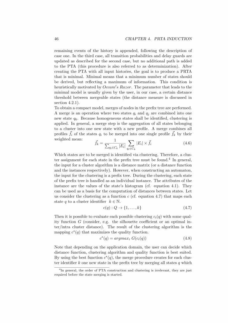
46 CHAPTER 4. PRTA INDUCTION
remaining events of the history is appended, following the description ofcase one. In the third case, all transition probabilities and delay guards areupdated as described for the second case, but no additional path is addedto the PTA (this procedure is also referred to as determinization). Aftercreating the PTA with all input histories, the goal is to produce a PRTAthat is minimal. Minimal means that a minimum number of states shouldbe derived, but reflecting a maximum of information. This condition isheuristically motivated by Occam′s Razor. The parameter that leads to theminimal model is usually given by the user, in our case, a certain distancethreshold between mergeable states (the distance measure is discussed insection 4.2.1).To obtain a compact model, merges of nodes in the prefix tree are performed.A merge is an operation where two states qi and qj are combined into onenew state qk. Because homogeneous states shall be identified, clustering isapplied. In general, a merge step is the aggregation of all states belongingto a cluster into one new state with a new profile. A merge combines allprofiles ~fi of the states qi to be merged into one single profile ~fk by theirweighted mean:
~fk =1∑
qi∈Ck|Ei|
∑qi∈Ck
|Ei| × ~fi (4.6)
Which states are to be merged is identified via clustering. Therefore, a clus-ter assignment for each state in the prefix tree must be found.4 In general,the input for a cluster algorithm is a distance matrix (or a distance functionand the instances respectively). However, when constructing an automaton,the input for the clustering is a prefix tree. During the clustering, each stateof the prefix tree is handled as an individual instance. The attributes of theinstance are the values of the state’s histogram (cf. equation 4.1). Theycan be used as a basis for the computation of distances between states. Letus consider the clustering as a function c (cf. equation 4.7) that maps eachstate q to a cluster identifier k ∈ N.
c(q) : Q→ {1, . . . , k} (4.7)
Then it is possible to evaluate each possible clustering ci(q) with some qual-ity function G (consider, e.g. the silhouette coefficient or an optimal in-ter/intra cluster distance). The result of the clustering algorithm is themapping c∗(q) that maximizes the quality function.
c∗(q) = argmaxi G(ci(q)) (4.8)
Note that depending on the application domain, the user can decide whichdistance function, clustering algorithm and quality function is best suited.By using the best function c∗(q), the merge procedure creates for each clus-ter identifier k one new state in the prefix tree by merging all states q which
4In general, the order of PTA construction and clustering is irrelevant, they are justrequired before the state merging is started.

4.1. PROBABILISTIC REAL-TIME AUTOMATA 47
are mapped to cluster k. Formally, the inverse function c−1(q)∗ returns foreach cluster identifier k the set of states that are mapped to it. The automa-ton is created by merging all states q of clusters k one after the other. Topreserve consistency, update operations on transitions have to be performed.If two states qi and qj are to be merged and there are no transitions tk wheretk = 〈qk, q′k, TLk
, φk, pk〉 and tl = 〈ql, q′l, TLl, φl, pl〉 with qk = ql, q
′k = qi and
q′l = qj (they do not share a predecessor), change tk to 〈ql, q′k, TLl, φl, pl〉
(re-link the transition) and compute the new profile of qi using equation4.1. qj can be deleted from the prefix tree. If there exist two transitions tkand tl with q′k = qi ∧ q′l = qj ∧ qk = ql (they share the same start but notend state), the transitions have to be merged additionally. This means that〈qk, q′k, TLk
, φk, pk〉 is to be updated to 〈qk, q′k, TLk, φ′k, pk + pl〉. φ′k = [a, b],
where a = min(φk, φl) and b = max(φk, φl).5 The updated probability p′ is
again calculated with the counts of the states p′ =|q′k|+|q
′l|
|qk| = pk + pl. Notethat the labels of the transitions are not updated until the end of the mergeprocedure. Then, each state holds its set of events and the labels TLk
can beeasily computed by calculating the difference between the two sets Ei andEj . Algorithm 6 shows this procedure.
Algorithm 6 CreateTransitionLabels (qi, qj)
for each ek ∈ Ei dofor each el ∈ Ej do
add δ(ek, el) to labels of transition t(qi, qj)end for
end for
One additional property of PRTAs is that a label δl ∈ TLkis only present
on exactly one outgoing transition of a state qi. Given that the underlyingdistance based clustering optimizes the inter and intra cluster distance, re-spectively, it can be shown that @ δl : δl ∈ TLk
∧ δl ∈ TLm . The proofworks by contradiction: consider the case where there exist three statesq0 = 〈{x1, x2}, f0〉, q1 = 〈{y1}, f1〉 and q2 = 〈{y2}, f2〉, with the transi-tions t1 = 〈q0, q1, δl, φ1, p1〉 and t2 = 〈q0, q2, δl, φ2, p2〉, i.e. two transitions,each holding label δl. Moreover, let δl be defined as δ(x1, y1), y1 /∈ E2 andy2 /∈ E1. Let us further assume, without loss of generality, that δl consistsof three consecutive blocks, e.g., δl = (+1 + 1 − 1 − 1000). Let k be thefirst position of the 0-block at the end. Following the assumption that δlexists on both transitions, we can specify constraints for x2 and y2. First,x1j := x2j and y1j := y2j for all j < k, because there is only one possibilityfor yj − xj to be equal to -1 (and 1) in a binary setting. Second, y2j := x2j
for j ≥ k, because otherwise δlj is not 0. Additionally, there must exists at
5In other words, we conduct the least general generalization on the time intervals tobe merged.

48 CHAPTER 4. PRTA INDUCTION
least one x1j 6= x2j to ensure that y2 6= y1. Otherwise, y1 and y2 are equaland thus clustered together, so t2 cannot exist. With these constraints: (1)x1j = x2j , y1j = y2j (i < k), (2) y2j := x2j (i ≥ k) and (3) y1 6= y2 thedistance d(x1, y1) reveals to be equal to d(x2, y2), because the distance forparts i ≤ k is 0 (2) and the remaining distances are equal (1). As y1 andy2 must reside in different clusters, the clustering then returns a solutionwhere pairs of objects with the same distance are clustered together once,and not a second time. This is inconsistent and also shows that the interand intra cluster distance in this clustering cannot be optimal. This leadsto the conclusion that for all suitable distance based clusterings there is noδl that occurs on more than one outgoing transition of one state q0. Finally,this conclusion even allows to check each learned automaton whether theintra cluster distances are above a threshold to ensure that each δl occursonly once.The delay guard generalization is motivated by the use of positive instancesonly. Remember that all input instances shall be accepted by the automa-ton, indicating that they are positive. Furthermore, we assume that whenno continuous timeframe is present in the data, it is not because it does notexist, but because of lack of data.6 However, the profiles of the states qi andqj have to be updated with their weighted mean. Transition tl is deleted.The same operations have to be applied on all outgoing transitions of statesqi and qj . After all merges are conducted, a quality measure of the cluster-ing is computed. Like in every clustering problem, the proportion of inter-and intra-cluster distances is of interest. The silhouette coefficient (SC) [47]evaluates this proportion independent of the number of resulting clustersand is a measure for the homogeneity of the states of the automaton. TheSC of a state qj representing a cluster C is calculated in the following way:
SCC =∑o ∈ C
b(o)− a(o)
max {a(o), b(o)}(4.9)
a(o) is the distance to the own cluster center, while b(o) denotes the distanceto the second next cluster center. The SC for the automaton is computedby averaging the SC for each state. It always holds that −1 ≤ SC ≤ 1.Good results are expected above an SC of 0.5. However, a high SC doesnot necessarily reflect the best clustering, since SCC = 1 for all |C| = 1 or|C| = X where X is the number of all instances. Generally, SCC increaseswith smaller clusters, because SCC = 1 for all states C that consist of oneexample only.The clustering method can be different for each use case. We decided tocluster with a divisive hierarchical cluster algorithm because it enables us to
6This assumption can be made in the medical application domain presented below.Here data is not recorded in regular time steps but whenever people go to the physician.So, there are gaps in the data recording process, which are taken into account by theabove assumption.

4.1. PROBABILISTIC REAL-TIME AUTOMATA 49
Figure 4.2: Example creation of a PRTA
define a distance threshold that has to be fulfilled by the clustering. Further-more, correlations between states can be investigated, and upper and lowerdistance thresholds can be set according to domain-specific constraints. Incontrast, it will not be possible to tell a priori how many states are to be ex-pected. This is why k-means like clustering methods are not appropriate inour scenario. Diana [47] is a divisive hierarchical clustering algorithm whichcomputes a final dendrogram that shows how ‘related’ the states are.7 Withthis dendrogram and a specific distance constraint, the user can create asuitable clustering. The dendrogram is cut according to the distance con-straint, and all objects that are still connected form a cluster. Nevertheless,one critical point for any clustering is to choose an appropriate distancemeasure. As this is domain-dependent, it will be discussed in the section onexperimental results.In Figure 4.2, a merge step during the construction of a PRTA is illustrated.We see here that the states are annotated with a profile and that transitionsconsist of all observed possibilities to end in a state, a path probability anda delay guard. The upper part of the figure displays three sample historiesin a prefix tree before the merging starts. For simplicity, the root of the pre-fix tree is not shown. The number in the states indicates to which clusterthe states belong to. Two of them are in cluster one, three are in clustertwo and only one state in cluster three. On all transitions only one event
7Preliminary experiments with a variety of other clustering algorithms like K-medoids[47], DBScan [5], EM, and Farthest First did not produce any usable results.

50 CHAPTER 4. PRTA INDUCTION
that leads from the left to the right state and the delay guard is displayed.A delay guard of [1,1] means that the event followed exactly one time stepafter the first event. The annotation of A2, A5, A6 on the transitions meansthat these attributes were observed after this state. The lower part of thefigure shows the automaton after the merging step (without the root). Thetransitions and delay guards are updated following the rules. The numberbehind the colon reflects the probability of this path. In this case, they arealways equal to one because there exists no splitting transition.
4.1.3 Predicting with an Automaton
In this section, we explain how such an automaton can be used to makepredictions. With a PRTA, we cannot only map processes that are reflectedin the data but also make predictions about how the next state of an instancewill be. Of course, it is also possible to predict series of subsequent states.The task of the prediction for a new instance can be formalized as follows:Given an instance x denoted by its feature vector ~fx = (f1, f2, . . . , fn), wewant to identify the profile ~f∗ = (f∗1 , f
∗2 , . . . , f
∗n) it will develop after l time
steps. A prediction for an instance is done by first identifying the state inthe PRTA that is most similar to the given event distribution of the instance.This is the start state qstart for the prediction:
qstart = argminqid( ~fx, ~fi) (4.10)
Distance function d will be introduced in a subsequent section. Given anarbitrary state q, let q1, . . . , qk denote the states with incoming transitionsfrom q, and p1, . . . , pk be the probabilities on those transitions. Moreover,let [t1,1, t1,2] to [tk,1, tk,2] denote the delay guards for the transitions. Thenthe predicted profile given l time steps starting with state q is defined as:
f∗(q, l) =∑ti,2>l
pi × fq +
∑ti,2≤l
pi × f∗(qi, l − ti,2)
The next state is predicted according to the transition probabilities andtheir delay guards. The first summand represents the case where state qis not left, because it consumes all the ‘remaining’ time. Thus, no otherfollowing state is considered for the prediction. The second sum representsthe case where the state has to be left. In the latter case, this means thatthe predicted profile of the next state is used. If q does not have any out-going transition, then f∗(q, d) = fq, i.e. the profile on the state itself. Toobtain a prediction for the test instance, we apply f∗ to qstart. Note that wemake the assumption that the automaton stays maximally long in a state,i.e. the transition is made as late as possible. Moreover, to leave a state,the delay guard has to meet the time constraint l: l > [tk,1, tk,2]. Then,

4.2. EXPERIMENTAL RESULTS 51
the remaining time l′ for the next steps is reduced by the maximum of thedelay guard l′ = l − ti,2. These constraints lead to a definite prediction ofthe profile: There is only one possible solution for the prediction. Anotherassumption would be that a transition is made as early as possible. Again,one definite prediction is achieved. However, an arbitrary time consumptionof each state could be desired as well. In this case, the prediction would bedependent on all (valid) possible time consumptions of each state. Accord-ingly, the prediction is the averaged profile of all resulting predictions. Usingthe later approach may result in an exponential number of possible resultsand a highly blurred predicted profile. That is why a definite predictionwas chosen in this chapter. However, the choice of a prediction constraint islikely to be highly domain-dependent. By calculating joint profiles, we canpredict the change of attributes depending only on the instance’s attributesetting. However, if one is interested in the development of a certain state,the automaton gives probabilities for future states. This is a main advan-tage of the automaton, because many comparable algorithms only give oneprediction. Consider a system that has alternatives for each state (e.g., med-ical therapy options and outcomes or biochemical pathways), meaning thata certain percentage of instances will take either the one or the other path.So, a distribution of resulting states is the desired output. The automatonaims at modeling such alternatives and their corresponding probabilities.
4.2 Experimental Results
In this section, we present the results of two experiments to test the algo-rithm. First, a proof of concept is conducted and subsequently an applica-tion to real-world medical data is presented to investigate the descriptiveand predictive power. Afterwards, a quantitative analysis of the algorithmis presented. Last, a comparison to Multi-Output HMMs is presented. Toadapt the approach to a given application, we now have to be more specificabout the distance measure used for clustering. Therefore, we first elaborateon such a measure for our medical application.
4.2.1 Distance Measure for Medical Applications
In general, every distance measure can be applied to the learning algorithmbut they should be adjusted to the application domain of interest. In the fieldof medicine, where an event reflects morbidities, the presence of a diseaseis more important than its absence, because the development of diseasesshall be explored. For this purpose, the design of a distance measure shallreflect that, when an attribute is present, it influences the distance strongerthan its absence. If it is absent, it means that the person does not sufferfrom a certain disease. This is further underlined by the fact that mostdiseases are comparatively rare. Most people of a population are healthy
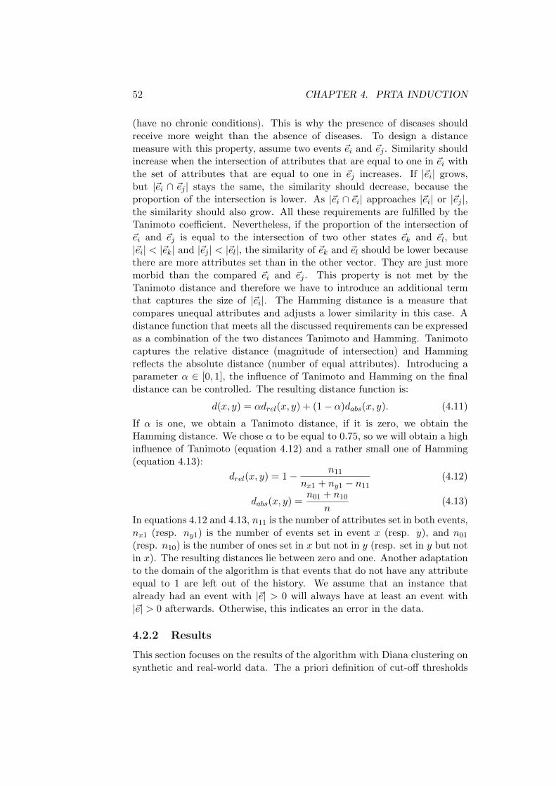
52 CHAPTER 4. PRTA INDUCTION
(have no chronic conditions). This is why the presence of diseases shouldreceive more weight than the absence of diseases. To design a distancemeasure with this property, assume two events ~ei and ~ej . Similarity shouldincrease when the intersection of attributes that are equal to one in ~ei withthe set of attributes that are equal to one in ~ej increases. If |~ei| grows,but |~ei ∩ ~ej | stays the same, the similarity should decrease, because theproportion of the intersection is lower. As |~ei ∩ ~ei| approaches |~ei| or |~ej |,the similarity should also grow. All these requirements are fulfilled by theTanimoto coefficient. Nevertheless, if the proportion of the intersection of~ei and ~ej is equal to the intersection of two other states ~ek and ~el, but|~ei| < |~ek| and |~ej | < |~el|, the similarity of ~ek and ~el should be lower becausethere are more attributes set than in the other vector. They are just moremorbid than the compared ~ei and ~ej . This property is not met by theTanimoto distance and therefore we have to introduce an additional termthat captures the size of |~ei|. The Hamming distance is a measure thatcompares unequal attributes and adjusts a lower similarity in this case. Adistance function that meets all the discussed requirements can be expressedas a combination of the two distances Tanimoto and Hamming. Tanimotocaptures the relative distance (magnitude of intersection) and Hammingreflects the absolute distance (number of equal attributes). Introducing aparameter α ∈ [0, 1], the influence of Tanimoto and Hamming on the finaldistance can be controlled. The resulting distance function is:
d(x, y) = αdrel(x, y) + (1− α)dabs(x, y). (4.11)
If α is one, we obtain a Tanimoto distance, if it is zero, we obtain theHamming distance. We chose α to be equal to 0.75, so we will obtain a highinfluence of Tanimoto (equation 4.12) and a rather small one of Hamming(equation 4.13):
drel(x, y) = 1− n11
nx1 + ny1 − n11(4.12)
dabs(x, y) =n01 + n10
n(4.13)
In equations 4.12 and 4.13, n11 is the number of attributes set in both events,nx1 (resp. ny1) is the number of events set in event x (resp. y), and n01
(resp. n10) is the number of ones set in x but not in y (resp. set in y but notin x). The resulting distances lie between zero and one. Another adaptationto the domain of the algorithm is that events that do not have any attributeequal to 1 are left out of the history. We assume that an instance thatalready had an event with |~e| > 0 will always have at least an event with|~e| > 0 afterwards. Otherwise, this indicates an error in the data.
4.2.2 Results
This section focuses on the results of the algorithm with Diana clustering onsynthetic and real-world data. The a priori definition of cut-off thresholds

4.2. EXPERIMENTAL RESULTS 53
and an evaluation of the predictive accuracy is presented. At first, a proofof concept is demonstrated. In this section the accuracy of the model interms of the number of states and transitions as well as their annotationis examined. Experiments on the real-world data sets give results of howmeaningful the automaton is from the application point of view, e.g. if thestructure reflects the known disease progressions and if it can predict futurestates correctly.
4.2.3 Proof of Concept
As described in Section 4.1 the induction of a PRTA is based on clustering.It therefore needs a distance constraint, indicating how similar events mustbe to form a cluster. This constraint is the cut-off in the dendrogram thatis returned by Diana clustering. As the correct structure of the automatonis known in this experimental setting, a lower and upper limit for the cut-off can be set. A cut-off of 0.3 would lead to a merge of states 5 and 9,which is not desired. To clarify this upper limit constraint, remember state5 ([2, 5, 6, 7, 8, 9]) and state 9 ([2, 5, 6, 7]). Their distance is composed of theTanimoto part (cf. equ. 4.12) which is equal to 1
3 and the Hamming contri-bution that is 0.2. Their weighted sum (according equation 4.11) is 0.3. Tofollow the requirement that they must not be merged, the cut-off must belower than 0.3. Additionally, it should also be greater than 0.21 to mergestate 2 ([1, 3, 4]) with a (possible) state that holds one additional attribute(e.g., [1, 2, 3, 4]). Thus a good automaton is expected with a cutoff between0.21 and 0.3. When exploring the resulting number of clusters and the SCfor the clustering in the interval between 0.26 and 0.3, a plateau of 10 statesand an SC of 0.97 arises. This indicates that a stable automaton can befound in this interval. For higher cut-offs, the number of clusters and theSC is dropping sharply. Lower cut-offs lead to more clusters that are purerbut do not incorporate exceptions in the states. The resulting automatonfor a cut-off of 0.3 is shown in Figure 4.3. It matches the true automatonstructure perfectly. There is only one exception in the structure. Thereexists a transition from state 2 to state 7 that is not present in the originalautomaton. This is due to the data. Remember that random errors wereintroduced in the data to check whether the automaton is able to find excep-tions in states. This causes state 2 to be followed by event [3,4,5] instead of[3,5] in one sequence. So event [3,4,5] matches the profile of state 7 ([3,4,5])perfectly and was merged with state 7 instead of state 3. Additionally, theSC shows that the states are homogeneous. The annotation of the statesin the PRTA shows that events ‘with errors’ were actually included in thestate. There are profiles that exhibit low frequencies of ‘wrong attributes’.However, this finding shows that the algorithm works correctly because ithas to group similar events. This makes the automaton less prone to dataerrors and produces stable results. Moreover, the user can identify the main

54 CHAPTER 4. PRTA INDUCTION
Figure 4.3: Results of algorithm on synthetic dataset. The layout is anal-ogous to Figure 4.2. Each node is labeled with an internal number that iscomputed by our implementation.
properties of a state and check how often an attribute occurs. The mainproperties of a state are those attributes that occur commonly, while excep-tions are all attributes that have a low frequency in a profile. Exceptionsmight be errors in the data but may also reflect rare cases in a system pro-gression. Finally, the probabilities on the transitions match those of theoriginal automaton quite well. We encounter at most a deviation of 0.15 inthe annotation of probabilities, where the largest deviations are apparentfor small transition probabilities. This experiment shows that the algorithmcan rediscover the correct structure of an automaton.To quantify the stability of the algorithm (not illustrated), we repeated thisexperiment 1000 times on different synthetic datasets that were obtainedfrom the predefined automaton. The correct number of states of the au-tomaton was induced in 31,8% of the cases, while in 50% of all runs theautomaton’s number of states resided between 10 and 12. Altogether, thenumber of states of the final automaton varies between 9 and 14 states. TheEuclidean distance of the induced states to their closest original lies between0 and 0.25, which indicates that the induced profiles are very similar to thetrue ones. The states that were identified worst are states 9 and 7, becausethey are very similar to states 5 and 3, respectively. This also led to a badidentification of the transitions of these states (only in about 50% of thecases), while the remaining transitions were almost always correctly iden-tified. These numbers indicate that the algorithm finds automata that arecorrect or very close to the original one.
4.2.4 Extraction of an Automaton on Real World Data

4.2. EXPERIMENTAL RESULTS 55
Results on diagnostic data To test our algorithm on real-world data, anautomaton was built on 1000 samples of the real-world diagnostic dataset.Again, a priori assumptions are needed to define an upper and lower boundfor the clustering cut-off. Here they were based on medical assumptions.States with |~e| = 1 (only one attribute is equal to one) shall not be mergedwith states where |~e| = 2. The motivation for this constraint is that in-dividuals with one disease shall be separated from those that have alreadyacquired two or more diseases and are thus multimorbid. This distinctioncan show the beginning and the progression of diseases and will help to in-terpret results. Furthermore, the cut-off should be set greater than zero.This constraint enables the automaton to merge states that are similar, butnot the same (due to errors in the recording of the data). This constraintcannot be fixed any further because the profiles of the resulting states arenot known in advance. Thus, meaningful automata are expected with a cut-off ≤ 0.4 . We computed the automaton for several cut-offs and extractedits corresponding silhouette coefficient (SC). As expected, the silhouette co-efficient drops as the cut-off increases. The higher the cut-off, the higher isthe variance in the clusters. This leads to an approximation of inter/intracluster distances and thus a reduction of the SC. However, it is interestingto notice that at a cut-off of 0.38 there is a sharp drop of the SC of aboutapproximately 18% and a drop of the number of clusters (20%). Therefore,one can assume that a meaningful cut-off threshold is reached and thus morestates are merged. The same behavior can be observed when we apply thealgorithm to only 100 instances. Therefore the cut-off 0.38 was chosen tocreate the PRTA. The resulting automaton contains 518 states and has anSC of 0.83.The first quality criterion of the automaton is its potential to reflect typicalmedical knowledge with its structure. The resulting automaton contains 19states that are highly connected to other states (also called hubs, cf. section4.2.5). They are mostly states with only one or two DGs (e.g., hyperten-sion and lung disease [e.g., COPD or asthma]). States like this are veryfrequent in the histories, so it is evident why those states are connected tomany others. Besides hubs, loops and paths are created. A loop is a pathin the automaton where start and end states are the same. The inspectedloops resemble individuals with multiple diseases (multimorbid), which donot change their general morbidities (e.g., diabetes, heart failure, hyperten-sion), but differ in their comorbidities (e.g., urologic disorders). Moreover,progression of diseases as well as improvements that reflect typical medical‘careers’ are present in the automaton. We conclude that the automatonshows meaningful medical patterns.A second quality parameter is the predictive power of the automaton. Toevaluate the predictive power of the algorithm, the dataset was split into atraining (75%) and a test (25%) set. The split was provided as part of anindustrial case study. For each of the k histories with n events of the test
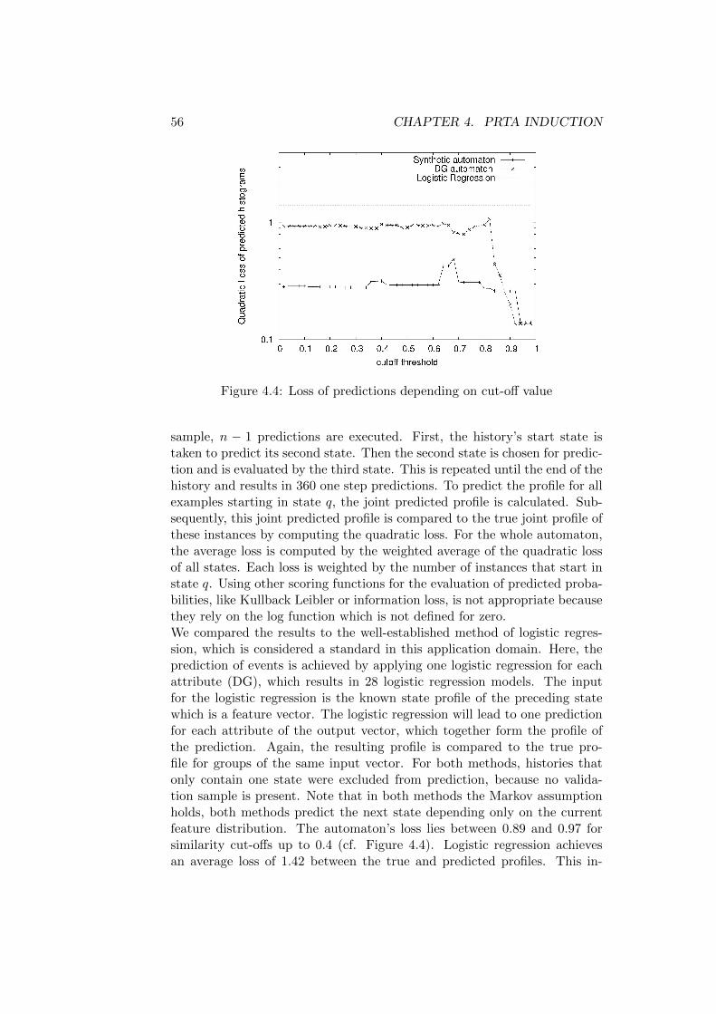
56 CHAPTER 4. PRTA INDUCTION
Figure 4.4: Loss of predictions depending on cut-off value
sample, n − 1 predictions are executed. First, the history’s start state istaken to predict its second state. Then the second state is chosen for predic-tion and is evaluated by the third state. This is repeated until the end of thehistory and results in 360 one step predictions. To predict the profile for allexamples starting in state q, the joint predicted profile is calculated. Sub-sequently, this joint predicted profile is compared to the true joint profile ofthese instances by computing the quadratic loss. For the whole automaton,the average loss is computed by the weighted average of the quadratic lossof all states. Each loss is weighted by the number of instances that start instate q. Using other scoring functions for the evaluation of predicted proba-bilities, like Kullback Leibler or information loss, is not appropriate becausethey rely on the log function which is not defined for zero.We compared the results to the well-established method of logistic regres-sion, which is considered a standard in this application domain. Here, theprediction of events is achieved by applying one logistic regression for eachattribute (DG), which results in 28 logistic regression models. The inputfor the logistic regression is the known state profile of the preceding statewhich is a feature vector. The logistic regression will lead to one predictionfor each attribute of the output vector, which together form the profile ofthe prediction. Again, the resulting profile is compared to the true pro-file for groups of the same input vector. For both methods, histories thatonly contain one state were excluded from prediction, because no valida-tion sample is present. Note that in both methods the Markov assumptionholds, both methods predict the next state depending only on the currentfeature distribution. The automaton’s loss lies between 0.89 and 0.97 forsimilarity cut-offs up to 0.4 (cf. Figure 4.4). Logistic regression achievesan average loss of 1.42 between the true and predicted profiles. This in-

4.2. EXPERIMENTAL RESULTS 57
state A46 A56 A58 A19 A80 A91 A83 A84 A86 A92 A131
1259 A46 A56 A19 A80 A91
1256 A46 A56 A58 A19 A80 A91
934 A46 A58 A19 A80 A91 A83 A84 A86 A92 A131
932 A19 A80 A91 A84 A86 A92 A131
835 A19 A80 A91 A83 A84 A86 A92 A131
929 A19 A80 A91 A84 A92 A131
Table 4.1: Example of the development of multimorbids: The features areas follows: A46 coagulation disorder, A56 psychosis, A58 depression, A19Diabetes, A80 heart failure, A91 hypertension, A83 heart attack, A84 coro-nary heart disease, A86 other heart problems, A92 arrhytmia, A131 renalfailure
dicates that the automaton may find better predictions than the logisticregression approach. Regarding the predictive power with higher cut-offs,the loss slightly increases but when the cut-off exceeds 0.8, the average lossquickly decreases again. This is because there are so many different statesin the clusters, that groups resembling the average population are created.Of course, they will also get predictions for the average population, which isbetter in the predictive power, but will not enable predictions on a personbut only on a group level. However, predicting the profiles for single personsis a main use case, and thus higher losses must be accepted. Compared tothe synthetic automaton, the real-world data automaton is worse in its pre-dictive power because it has more attributes and a higher variability in thestates and histories. The synthetic automaton has quite the same predictiveratio at each cut-off because of the small variability in the data. So, smallerpredictive errors can be observed for the synthetic automaton. Initial exper-iments on the prediction accuracy showed that for smaller testsets (e.g. ina 10fold cross validation setting) the average prediction accuracy decreases.This may be caused by the fact that neither in the true test set nor in theprediction the average population profile is computed but only a fractionof all possible profiles are considered. Thus the variation is high and thedifference between the true and predicted profile may increase. However, adetailed exploration of the predictive power remains for future work.
Investigating patterns of a (real-world) diabetes automaton Inthis paragraph we illustrate the medical knowledge represented by an au-tomaton. We focus on a qualitative evaluation, not on a quantitative at thispoint. An automaton for patients suffering from diabetes was created on 100randomly sampled patients. The data was available for 4 years and stateswere derived on a half-year basis. One state comprises data from quartertwo and three of a year or quarter four and the subsequent first quarter, forseasonal reasons. Only frequent (occurring in more than 5% of all patients)
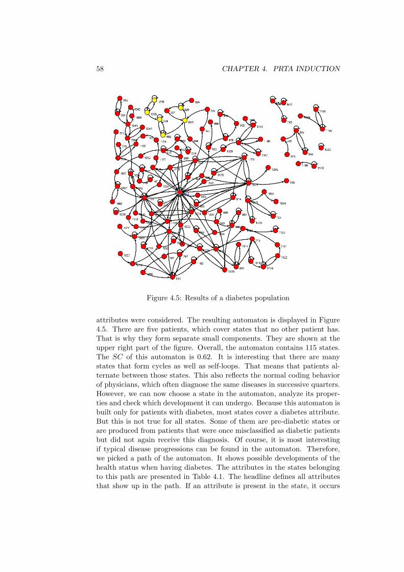
58 CHAPTER 4. PRTA INDUCTION
Figure 4.5: Results of a diabetes population
attributes were considered. The resulting automaton is displayed in Figure4.5. There are five patients, which cover states that no other patient has.That is why they form separate small components. They are shown at theupper right part of the figure. Overall, the automaton contains 115 states.The SC of this automaton is 0.62. It is interesting that there are manystates that form cycles as well as self-loops. That means that patients al-ternate between those states. This also reflects the normal coding behaviorof physicians, which often diagnose the same diseases in successive quarters.However, we can now choose a state in the automaton, analyze its proper-ties and check which development it can undergo. Because this automaton isbuilt only for patients with diabetes, most states cover a diabetes attribute.But this is not true for all states. Some of them are pre-diabetic states orare produced from patients that were once misclassified as diabetic patientsbut did not again receive this diagnosis. Of course, it is most interestingif typical disease progressions can be found in the automaton. Therefore,we picked a path of the automaton. It shows possible developments of thehealth status when having diabetes. The attributes in the states belongingto this path are presented in Table 4.1. The headline defines all attributesthat show up in the path. If an attribute is present in the state, it occurs
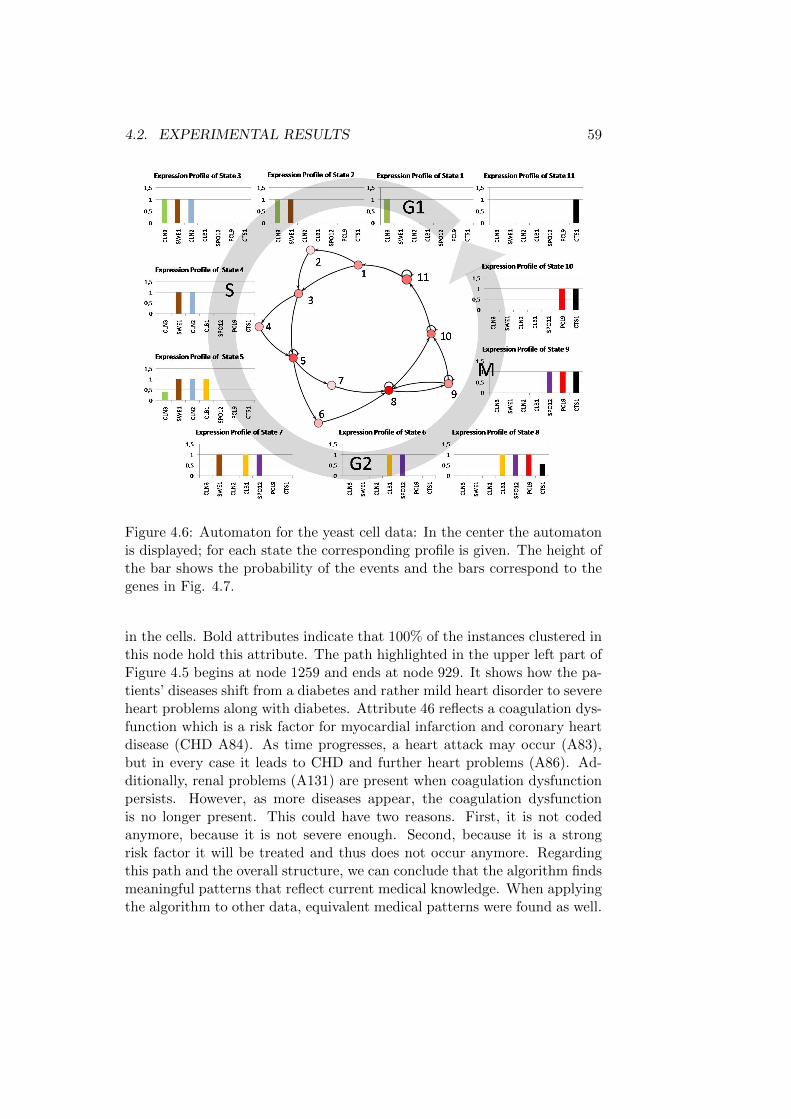
4.2. EXPERIMENTAL RESULTS 59
Figure 4.6: Automaton for the yeast cell data: In the center the automatonis displayed; for each state the corresponding profile is given. The height ofthe bar shows the probability of the events and the bars correspond to thegenes in Fig. 4.7.
in the cells. Bold attributes indicate that 100% of the instances clustered inthis node hold this attribute. The path highlighted in the upper left part ofFigure 4.5 begins at node 1259 and ends at node 929. It shows how the pa-tients’ diseases shift from a diabetes and rather mild heart disorder to severeheart problems along with diabetes. Attribute 46 reflects a coagulation dys-function which is a risk factor for myocardial infarction and coronary heartdisease (CHD A84). As time progresses, a heart attack may occur (A83),but in every case it leads to CHD and further heart problems (A86). Ad-ditionally, renal problems (A131) are present when coagulation dysfunctionpersists. However, as more diseases appear, the coagulation dysfunctionis no longer present. This could have two reasons. First, it is not codedanymore, because it is not severe enough. Second, because it is a strongrisk factor it will be treated and thus does not occur anymore. Regardingthis path and the overall structure, we can conclude that the algorithm findsmeaningful patterns that reflect current medical knowledge. When applyingthe algorithm to other data, equivalent medical patterns were found as well.

60 CHAPTER 4. PRTA INDUCTION
Results yeast metabolism data In this paragraph, another applicationbased on yeast cell data is presented. It will illustrate how automata can beused to infer knowledge about biological processes. In this experiment, geneexpression data of the budding yeast is modeled by an automaton, which isdisplayed in Figure 4.6. It consists of 11 states and 21 transitions with anSC of 0.87. The cutoff was set to 0.224. It was derived by the fact thatdue to the quite low number of attributes, states shall be very pure (anddistinct) and thus merges shall be allowed only when there are at least fourattributes in a state, which is more than half of all attributes. Inspectingthe structure of the automaton, the most apparent fact is that it is a cycle.Thus, the automaton presents a periodic pattern that the organism passesthrough, which can also be discovered in the original data. This is knownto be the cell cycle of the budding yeast. In a well nourished culture, yeastgrows and divides in a constant manner. The process is divided into fourcoarse steps: the G1, S, G2 and M phase. During the G1 phase the cell isgrowing, and then the DNA is duplicated in the S phase. Subsequently, thecell prepares for division in the G2 phase and finally divides in the M phase.In each phase specific genes are expressed that control the processes of thecell. Investigating the expression profiles of each state in the automaton,specific expression profiles can be found. Comparing these profiles to knownactivation gene patterns (cf. Figure 4.7 upper part), the stages of the cellcycle can be annotated to the states [74]. The profiles show that each geneis expressed at a specific stage and that genes also have a specific temporalordering. Most importantly, state 1 represents the start of a cell cycle andstate 11 is its end.But not only the structure of observed biological processes, also temporalcharacteristics can be reflected by the automaton. Usually, cells rest sometime after a division, which leads to a lag before the next cell cycle starts.This prolonged resting phase is captured by the delay guard on the transitionfrom state 11 to state 1. It does not only allow for immediate transitions butalso a delayed transition after two time steps. Moreover, stages lasting morethan one time step (e.g., G2) can be visited more than once, representedby a self loop. This means that the cell stays in a state for a while. Addi-tionally the automaton captures the possibility that expression peaks/dropsmay occur faster or slower. These alternatives are illustrated by, e.g. thetransition from state 5 to 8 via state 6 or 7 respectively. While state 7 stillholds gene SWE1, it is not present in state 6, which shows that here theexpression rate has dropped faster than in the former case. Comparing thisto the original data in Figure 4.7, the quick drop of gene SWE1 can be seenat timeframe 11 to 13, while a slower drop occurs in timeframe 22 to 26.Such an alternative is also presented in the transition from state 1 to state3 (traversing state 2 potentially). The direct connection shows that genesSWE1 and CLN2 are expressed at the same time, while state 2 shows thatgene SWE1 comes first. However, the probabilities on the transitions indi-
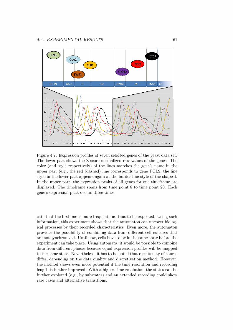
4.2. EXPERIMENTAL RESULTS 61
Figure 4.7: Expression profiles of seven selected genes of the yeast data set:The lower part shows the Z-score normalized raw values of the genes. Thecolor (and style respectively) of the lines matches the gene’s name in theupper part (e.g., the red (dashed) line corresponds to gene PCL9, the linestyle in the lower part appears again at the border line style of the shapes).In the upper part, the expression peaks of all genes for one timeframe aredisplayed. The timeframe spans from time point 8 to time point 20. Eachgene’s expression peak occurs three times.
cate that the first one is more frequent and thus to be expected. Using suchinformation, this experiment shows that the automaton can uncover biolog-ical processes by their recorded characteristics. Even more, the automatonprovides the possibility of combining data from different cell cultures thatare not synchronized. Until now, cells have to be in the same state before theexperiment can take place. Using automata, it would be possible to combinedata from different phases because equal expression profiles will be mappedto the same state. Nevertheless, it has to be noted that results may of coursediffer, depending on the data quality and discretization method. However,the method shows even more potential if the time resolution and recordinglength is further improved. With a higher time resolution, the states can befurther explored (e.g., by substates) and an extended recording could showrare cases and alternative transitions.

62 CHAPTER 4. PRTA INDUCTION
(a) Structure for different cutoffs (b) Number of states for different input datasizes
(c) Structure for different input data sizes (d) Resulting loss with different input datasizes
Figure 4.8: Structural dependencies for different cutoffs and numbers ofinput data
4.2.5 Empirical Evaluation
In this section, some empirical properties of the algorithm are explored. Thebehavior depending on its main parameters, the number of histories (inputsequences) and cut-off values, are studied in detail. Additionally, a runtimeanalysis will be presented. First, the correlation between the number ofstates (and other structural features) and increasing cut-offs of the clusteringwill be shown. Second, an investigation of those features depending on thenumber of input sequences is presented.
Cut-off Dependencies
To evaluate the structural features of the resulting automata, the number ofhubs, singletons, dead ends and start states relating to the cut-off is presented(cf. Fig. 4.8a). We define a hub as a state that has transitions to at least10% of the remaining states in the automaton. Singletons are states thatdo not have a transition to another node. Start and dead end states onlyhave outgoing and incoming edges respectively. With an increasing cut-

4.2. EXPERIMENTAL RESULTS 63
off, similar states are clustered and therefore the number of hubs increasesas well. This is because the number of states drops while the number oftransitions stays constant. However, for the highest cut-offs the numberof hubs drops again, because even hubs are combined into fewer states.Singletons become fewer with increasing cut-off. Again, they are mergedwith other states that have a connection to other states and thus they areno singletons no more. The same is true for dead end states. The numberof states in the final automaton drops linearily (after a cut-off of 0.1) as thecut-off of the hierarchical clustering increases (not shown). For cutoff valuesgreater than 0.9, only one state appears in the resulting automaton. Thereason for this is that with a higher cut-off, states that are less similar willbe clustered and thus form fewer states.
Dependency on the Number of Input Sequences
Figures 4.8b to 4.8d show how the number of input sequences affects the re-sulting automaton. In Figure 4.8b, the number of final states in the resultingautomaton is shown. It is interesting to note that the number of states doesnot grow linearly but seems to converge to an upper limit. This may be ex-plained by rare disease characteristics which are only present after a certainsample size. For low sample sizes, many frequent patterns are discoveredand so the number of states increases rapidly. But subsequently, mostlyrare cases are incorporated into the model, which leads to a slower growthrate of the automaton. However, the final number of states should then notsignificantly increase further. Regarding the number of hubs, Figure 4.8cshows that with an increasing number of input sequences the number ofhubs (left axis) that appear in the final automaton is quite stable. Keepingin mind that a hub occurs when a state is connected to more than 10% ofthe remaining states, this indicates that a certain number of disease statesfrequently appear in the histories. This can be true for, e.g. a ‘hyperten-sion’ diagnosis or a metabolic problem, which are both frequent, alone andin combination with other diseases. The frequency of singletons, dead endsand start states (right axis) drops with an increasing number of input se-quences. That indicates that even rare cases are observed more frequentlyand therefore occur in more sequences, which leads to a higher transitionrate in these states. Finally, the quadratic loss of the predicted histogramswith a growing number of input data is evaluated. The results of theseexperiments are illustrated in Figure 4.8d. The calculated interpolation ofthe data points indicates that the overall loss of the predicted histogramsdecreases with more input data. This can be explained by the inclusion ofrarer cases which only appear in larger datasets. Thus, events that needrare information can be predicted more accurately.

64 CHAPTER 4. PRTA INDUCTION
IS 50 100 200 400 600 800 1000
RT (s) 4 3 6 23 60 120 240
Table 4.2: Runtime (RT) depending on number of input sequences (IS)
Runtime Evaluation
We determined the runtime for a varying number of input sequences. Allexperiments were conducted on a 1.7GHz machine with 2GB RAM wherethe PRTA is implemented in Java with an interface to R and Weka to usethe clustering algorithms. As Table 4.2 shows, PRTAs can be created withinacceptable time frames. The runtime of the algorithm is mainly impactedby the clustering method. So, the decision for one or the other clusteringmethod can result in significantly higher or lower running times. As Dianaclustering is used in this approach, the runtime is bounded by O(n2). Thisis also reflected in Table 4.2, where the runtime is illustrated.
4.2.6 Comparison with an Multi-Output HMM
Although HMMs do not provide multi-attribute structure learning, a com-parison of the automaton to a Multi-Output HMM (MOHMM) [10] is pre-sented here, which is a special case of DBNs [38]. We used the implemen-tation in MoCaPy8 to create a state-space HMM that allows to be trainedwith 28-dimensional input vectors. The result is a 28-dimensional outputvector described by 28 discrete output nodes. The output nodes are onlydependent on the hidden node in one slice. The structure was chosen apriori, following a suggestion by one of the developers. Because we assumeindependence of attributes, no dependencies in the output layer were intro-duced. Furthermore, because the prediction is only dependent on the givenevent, one hidden node per slice is considered appropriate. The MOHMMwas trained on the disease group data with exactly the same training andtest sets as the ones for the automaton. To look for the best possible so-lution, we changed the internal node size of the hidden node from 2 to 50.The resulting loss is shown in Table 4.3. We calculated the prediction by a500-fold sampling of the MOHMM and selected the sequence with the bestlog likelihood. Again, the quadratic loss was computed. The best predic-tion was achieved with a node size of 20 which resulted in a quadratic loss of3.22. This is due to the fact that the MOHMM has a higher probability ofpredicting the presence of attributes, although they are not observed in thedata. Additionally, the internal node size allows for more variables whichat first improves the loss but eventually causes the performance to degradeslightly. To explore how the loss depends on the number of nodes per slice,MOHMMs with 2 and 3 nodes per slice were computed and evaluated as
8http://sourceforge.net/projects/mocapy/
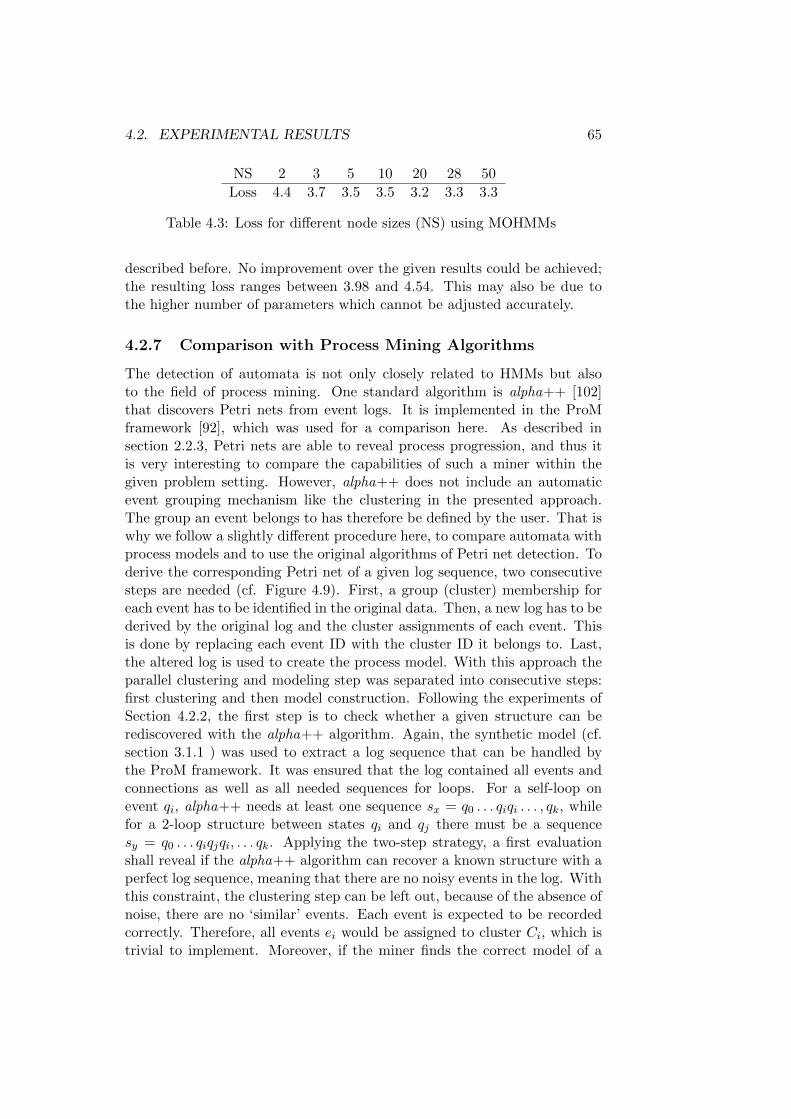
4.2. EXPERIMENTAL RESULTS 65
NS 2 3 5 10 20 28 50
Loss 4.4 3.7 3.5 3.5 3.2 3.3 3.3
Table 4.3: Loss for different node sizes (NS) using MOHMMs
described before. No improvement over the given results could be achieved;the resulting loss ranges between 3.98 and 4.54. This may also be due tothe higher number of parameters which cannot be adjusted accurately.
4.2.7 Comparison with Process Mining Algorithms
The detection of automata is not only closely related to HMMs but alsoto the field of process mining. One standard algorithm is alpha++ [102]that discovers Petri nets from event logs. It is implemented in the ProMframework [92], which was used for a comparison here. As described insection 2.2.3, Petri nets are able to reveal process progression, and thus itis very interesting to compare the capabilities of such a miner within thegiven problem setting. However, alpha++ does not include an automaticevent grouping mechanism like the clustering in the presented approach.The group an event belongs to has therefore be defined by the user. That iswhy we follow a slightly different procedure here, to compare automata withprocess models and to use the original algorithms of Petri net detection. Toderive the corresponding Petri net of a given log sequence, two consecutivesteps are needed (cf. Figure 4.9). First, a group (cluster) membership foreach event has to be identified in the original data. Then, a new log has to bederived by the original log and the cluster assignments of each event. Thisis done by replacing each event ID with the cluster ID it belongs to. Last,the altered log is used to create the process model. With this approach theparallel clustering and modeling step was separated into consecutive steps:first clustering and then model construction. Following the experiments ofSection 4.2.2, the first step is to check whether a given structure can berediscovered with the alpha++ algorithm. Again, the synthetic model (cf.section 3.1.1 ) was used to extract a log sequence that can be handled bythe ProM framework. It was ensured that the log contained all events andconnections as well as all needed sequences for loops. For a self-loop onevent qi, alpha++ needs at least one sequence sx = q0 . . . qiqi . . . , qk, whilefor a 2-loop structure between states qi and qj there must be a sequencesy = q0 . . . qiqjqi, . . . qk. Applying the two-step strategy, a first evaluationshall reveal if the alpha++ algorithm can recover a known structure with aperfect log sequence, meaning that there are no noisy events in the log. Withthis constraint, the clustering step can be left out, because of the absence ofnoise, there are no ‘similar’ events. Each event is expected to be recordedcorrectly. Therefore, all events ei would be assigned to cluster Ci, which istrivial to implement. Moreover, if the miner finds the correct model of a

66 CHAPTER 4. PRTA INDUCTION
Figure 4.9: Illustration of the sequential approach. In the upper left corner,the original input sequences are displayed. Events are first clustered (right)by treating each event of the sequence as an individual instance. Again,a mapping of each event to a cluster identifier is achieved. By using thismapping and the sequence information of the original data, a dataset asinput for a process miner can be derived (lower left part): In each sequencethe event identifier is replaced by the corresponding cluster identifier.
noise-free log, it will also be able to find the correct structure in a noisy logwith a preceding clustering. In this case, the quality of the model is mainlydependent on the clustering and not of the alpha++ algorithm itself.The alpha++ algorithm was applied to noise-free synthetic data; its result-ing Petri Net is displayed in Figure 4.10 B. Inspecting the model, thereare two main errors. Transition9 2 and 5 are not at all connected to othertransitions. There is only one connection to the start place (and end placerespectively). Second, there is a connection from state 7 to the input placeof 6 and 4. This indicates that 4 may come after 7, which is neither indicatedin the model nor in the log. The reason why alpha++ places this connectionis that there is no other possibility to connect 6 and 7 without risking thatmarkers may become stuck in the net (e.g., by inserting an additional placebetween 6 and 7). This requirement is induced by the demand that only
9In the field of Petri nets, states are called transitions. They model discrete events.Events are connected via places that describe conditions. They enable transitions viamarkers that are produced and consumed in the net. Transitions are displayed as rectan-gles, places as circles.

4.2. EXPERIMENTAL RESULTS 67
Figure 4.10: Resulting models using alpha ++ (B) and alpha # (C) com-pared to the given synthetic model (A)
valid Petri nets shall be discovered. Moreover, in the alpha++ algorithmthere is no check if invalid connections exist. This leads for example to theconnections between 8, 9 and 10 where all required connections are modeledbut there is now an additional direct connection between 8 and 10, which isnot present in the original model. In fact, this misplacement can be handledby the alpha # algorithm [103]. It was designed to detect invisible tasksthat can model SIDE, SKIP, REDO and SWITCH constructs. To check thebeneficial impact of the invisible tasks, alpha # was subsequently applied tothe same log. The resulting Petri net is displayed in Figure 4.10 C, wherewhite rectangles are invisible tasks. It shows major improvements over thefirst Petri net: state 2 and 5 are included correctly, the connections between8, 9 and 10 are correctly discovered and the wrong connection from 7 to 4is left out. Nevertheless, there are errors as well. First, connections fromand to transition 4 are missing. Only 3 to 4 and 4 to 5 are included in themodel. Both two-loop structures between 1 and 4 as well as 4 and 10 arecompletely missing in the Petri net, although these connections were actu-ally present in the log. Alpha # here fails to assign the correct connections.This is a serious error, because the model is simply incorrect and moreover,such two-loop structures are frequently present in the underlying domain(cf. Figure 4.5 for examples). Second, the Petri net is quite confusing dueto many invisible tasks that were inserted to model all dependencies. Thiscan be illustrated by looking for the self loop of transition 5. It is indeed

68 CHAPTER 4. PRTA INDUCTION
present in the model but stretches over two invisible tasks and thus maynot be practical for users to infer information about unknown systems. Thesame can be detected at the 8 to 5 connection. Such connections can easilybe overlooked or even misinterpreted by the user.Summarizing these results, both algorithms are not able to correctly reveal aknown structure in the domain of automata detection. The main reason forthis is that they are designed to detect discrete distributed systems. Theirmain purpose is to model parallelism in a quite linear ordering, which mightnot be given in a more complex system. Additionally, Petri nets have to sat-isfy constraints regarding liveliness, reachability and boundedness. InducedPetri nets should avoid dead transitions and thus exclude desired connec-tions or over-generalize, respectively. To provide the same possibilities as inthe presented automaton, all transitions should be reachable from the startplace. This will allow the modeled system to enter at arbitrary states. Todo so, there must be a connection from the start place to each transition inthe Petri net. This is only possible, if each event is at least once the firstevent in a history, which cannot be guaranteed a priori. A further questionis how to model probabilities on connections. Consider the input place of 5in Figure 4.10 C. There are four possibilities of how the input place can bereached from other transitions. However, there is only one connection fromthe place to transitions 5. Thus, the transition can only be labeled withone event. If delay guards and probabilities of the incoming connections aredifferent, it cannot be properly deployed on one connection, because oncethe place was visited, one cannot decide which connection was used. In con-trast, making small modifications, labeling of definite connections would bepossible as well as the annotation of transitions with profiles. Regarding alldiscussed issues, we can conclude that Petri nets first do not always discoverall dependencies of events in complex systems (as in the presented medi-cal domain), and second, are not yet adapted to handle varying transitionprobabilities of precedent events, while still satisfying the standard modelconstraints. Due to these limitations, Petri nets cannot yet be used for thegiven problem statement.
4.3 Conclusion
In this chapter, we proposed a new method for learning process modelsin the form of probabilistic real-time automata (PRTA) for multi-attributeevent logs. To learn such models, a prefix tree is created, in which statesare merged when similar enough. State merging is employed because it iscurrently the best method for learning finite automata in grammatical in-ference [27]. In order to identify states to be merged, a divisive hierarchicalclustering method is used. The algorithm was evaluated on synthetic data,for which the true underlying process was known. Moreover, it was tested

4.3. CONCLUSION 69
on real data from a medical and a biological application domain to examinethe resulting structure. The experiments showed that the automaton, inparticular its hubs, paths and loops, but also its overall structure, can berelated to domain knowledge. To compare the ability of structure identifica-tion, standard process mining algorithms were applied on the same syntheticdata set. However, they were not able to reveal the correct structure of theunderlying process, because of the additional constraints they have to fulfill.Finally, to evaluate the predictive power of the PRTA, the distance of thepredicted profiles to the profiles of the true next states was computed. Thepredictions of the PRTA were compared to the predictions of a combined lo-gistic regression approach, which is considered a standard in this applicationdomain. Additionally, a Multi-Output HMM was trained and tested for itspredictive power. The results suggest that the automaton-based predictionperforms favorably compared to both logistic regression and Multi-OutputHMMs. In the future, we want to further explore the automaton’s proper-ties (like the stability, representation of domain knowledge and predictivepower) depending on different dataset characteristics. Moreover, we wouldlike to investigate the use of pattern mining techniques for the creation ofstates (cf. Chapter 5 and 9) and the annotation of states by predicates [49].

70 CHAPTER 4. PRTA INDUCTION
Chapter 5
Scalable Induction ofProbabilistic Real TimeAutomata (SPRTA)
The induction of real time automata (RTA) was introduced recently [96,95, 97] and is currently based on a state merging procedure. The PRTA(cf. Chapter 4 [81]) is derived from this type of automaton, but additionallyincludes profiles and transition labels as well as transition probabilities inthe model. Thus, it is able to handle multi-attribute event logs, contrary toRTAs. This enables modelling organism or population development insteadof only the relation between, e.g. genes or organisms. To induce a PRTA, thestate merging procedure uses the result of a prior clustering step (DIANA[40]). DIANA is a batch clusterer and performs best compared to a varietyof other cluster algorithms like k-Medoids, DB-Scan and EM that have alsobeen considered for the induction of automata [81]. DIANA is the onlyclustering algorithm that was able to induce reasonable results, i.e., findmore than one cluster, without using a predefined cluster number, but onlyrelying on a distance constraint. Moreover, so far no clustering with asymbolic description (e.g., frequent patterns) was applied to the induction ofautomata. In contrast, in the field of regular clustering, there are examplesthat also group time series data where the final clusters have a symbolicdescription [31]. The clustering is achieved in a two-step process: first, alocal pattern mining method constructs patterns on the attributes of theinstances. These patterns are then used to construct predictive clusteringtrees (PCTs). Next to that, Itemset Constrained Clustering (IC-Clustering)[85] finds clusters having an itemsets description. It uses a branch and boundapproach to come up with its results. Co-clustering (bi-clustering, formalconcepts) also finds clusters of objects that share frequent patterns andwas intensively explored for the standard setting of binary data [7], n-aryrelations [15], numeric data sets [70] and useful applications [8]. In graph
71
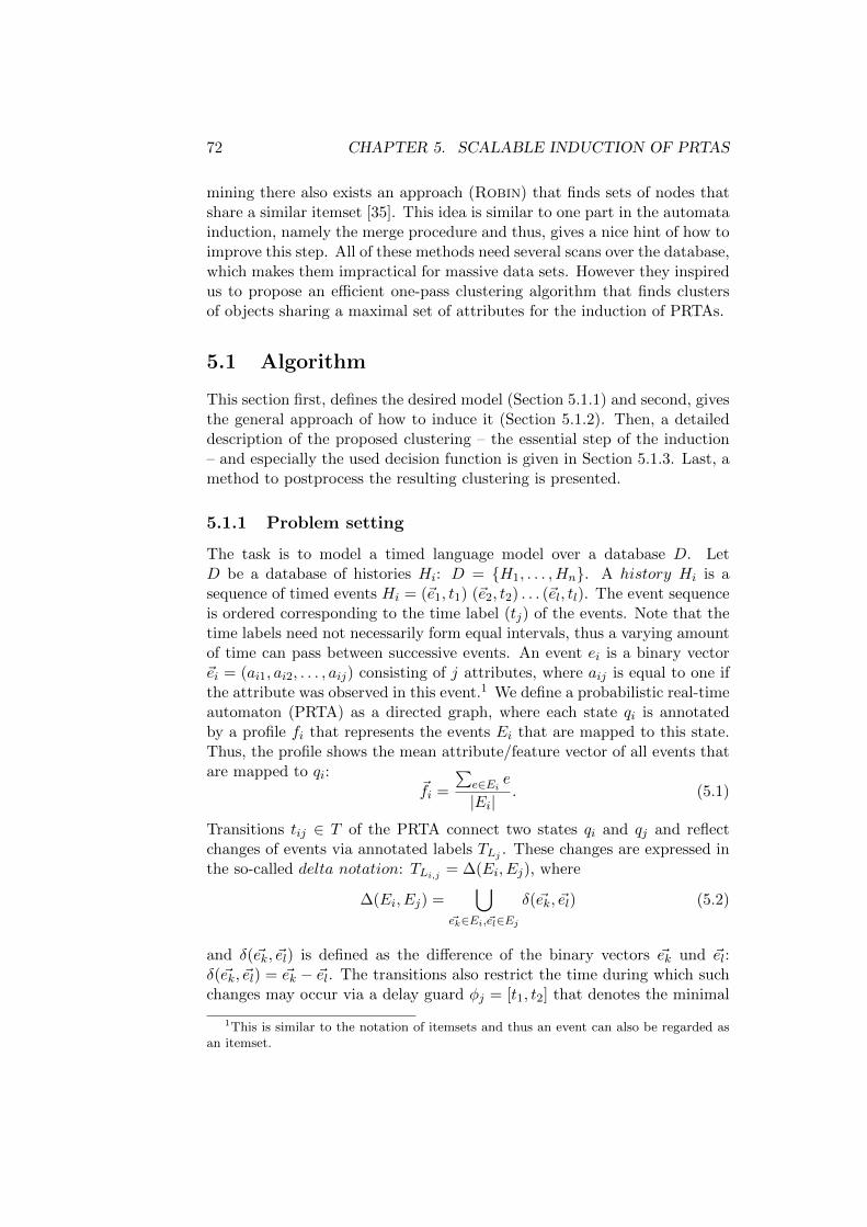
72 CHAPTER 5. SCALABLE INDUCTION OF PRTAS
mining there also exists an approach (Robin) that finds sets of nodes thatshare a similar itemset [35]. This idea is similar to one part in the automatainduction, namely the merge procedure and thus, gives a nice hint of how toimprove this step. All of these methods need several scans over the database,which makes them impractical for massive data sets. However they inspiredus to propose an efficient one-pass clustering algorithm that finds clustersof objects sharing a maximal set of attributes for the induction of PRTAs.
5.1 Algorithm
This section first, defines the desired model (Section 5.1.1) and second, givesthe general approach of how to induce it (Section 5.1.2). Then, a detaileddescription of the proposed clustering – the essential step of the induction– and especially the used decision function is given in Section 5.1.3. Last, amethod to postprocess the resulting clustering is presented.
5.1.1 Problem setting
The task is to model a timed language model over a database D. LetD be a database of histories Hi: D = {H1, . . . ,Hn}. A history Hi is asequence of timed events Hi = (~e1, t1) (~e2, t2) . . . (~el, tl). The event sequenceis ordered corresponding to the time label (tj) of the events. Note that thetime labels need not necessarily form equal intervals, thus a varying amountof time can pass between successive events. An event ei is a binary vector~ei = (ai1, ai2, . . . , aij) consisting of j attributes, where aij is equal to one ifthe attribute was observed in this event.1 We define a probabilistic real-timeautomaton (PRTA) as a directed graph, where each state qi is annotatedby a profile fi that represents the events Ei that are mapped to this state.Thus, the profile shows the mean attribute/feature vector of all events thatare mapped to qi:
~fi =
∑e∈Ei
e
|Ei|. (5.1)
Transitions tij ∈ T of the PRTA connect two states qi and qj and reflectchanges of events via annotated labels TLj . These changes are expressed inthe so-called delta notation: TLi,j = ∆(Ei, Ej), where
∆(Ei, Ej) =⋃
~ek∈Ei,~el∈Ej
δ(~ek, ~el) (5.2)
and δ(~ek, ~el) is defined as the difference of the binary vectors ~ek und ~el:δ(~ek, ~el) = ~ek − ~el. The transitions also restrict the time during which suchchanges may occur via a delay guard φj = [t1, t2] that denotes the minimal
1This is similar to the notation of itemsets and thus an event can also be regarded asan itemset.

5.1. ALGORITHM 73
and maximal time steps when this transition can be passed. Moreover, atransition is annotated with a probability pj of occurrence. The sum of theprobabilities of all outgoing transitions of one state is equal to one.
Definition A PRTA Γ is a tuple Γ = (Q,∑, T, S, F )
• Q is a finite set of states
• Σ is a finite set of events to label the transitions
• T is a finite set of transitions
• S = Q is the set of start states
• F = Q is the set of final states
A state qi ∈ Q is a pair 〈Ei, ~fi〉 where Ei is its set of events and ~fi is anattribute vector called its profile. Σ are all events ~e that are observed in D.A transition t ∈ T is a tuple 〈q, q′, TL, φ, p〉 where q, q′ ∈ Q are the sourceand target states, TL is its label and φ is a delay guard defined by an interval[t1, t2] with t1, t2 ∈ N. p defines the probability p ∈ [0, 1] that this transitionoccurs. The goal is to induce a probabilistic real time automaton Γ thatmodels D and is minimal. Minimal means that the least number of stateswith respect to some parameter setting must be found [81, 96].
5.1.2 Basic Algorithm
In this section, the basic algorithm for the creation of a PRTA is explained.Algorithm 7 shows the subsequent steps of the approach which is furtherillustrated in Figure 5.1. The main steps of the induction are (1) the creationof a prefix tree acceptor, (2) the clustering of the nodes of the PTA and (3)the merge of all nodes in a cluster. In the following each step is explainedin more detail.
1. The PRTA is induced by first creating a prefix tree acceptor (PTA)[95, 81]. A PTA is a tree of histories, where shared history prefixesare merged to one path. Thus, each node si ∈ PTA corresponds to aset of events Ei. Moreover, a profile is added to each node in the PTAwhich is equal to Ei. Note that during the PTA creation the data setis only accessed once, while the remaining steps are conducted on thePTA itself. Therefore, the performance is mainly dependent on thefollowing steps.
2. After the PTA creation, the next step is to cluster the nodes of thePTA. In this chapter, we propose to use an online clustering methodfor this task, for which the motivation is now briefly described andfurther explained in detail in Section 5.1.3. To cluster the nodes ofthe PTA, each node si of the PTA is treated as an individual instance,

74 CHAPTER 5. SCALABLE INDUCTION OF PRTAS
Figure 5.1: General overview of the PTA creation. Top: input data - aset of histories consisting of multi-attribute events. The black and whiteboxes indicate a binary event (α, β or γ). An event is fully described by thisbinary feature vector. Bottom: successive steps of the PRTA creation. Firsta PTA is created (left) and then its nodes are clustered (middle). Relyingon this clustering, the nodes of the PTA are merged to form the final states(right). For state 1 the profile and for transition t1,2 the delay guard andthe probability are given, exemplarily.
for which a decision function fNC(si, C) (presented in Section 5.1.3)identifies whether si belongs to a cluster Cj in the current clusteringC (Alg.7, line 4). If this is the case (k 6= −1), then the instance isadded to cluster Cj (cf. line 6). Otherwise, a new cluster is createdand instance si is put into the new cluster (cf. line 8). The functionfNC(si, C) that decides whether an instance belongs to a cluster isbased on the following basic idea: The instance is to be placed in thatcluster whose maximal frequent patterns (MFPs) best cover the newinstance. Then, all instances in a cluster share a maximal amount ofproperties and are thus very similar. As usual, a pattern is frequent ifits frequency exceeds a minimum support threshold of θ and maximalif it is not a subset of another frequent pattern [40]. For the givenproblem setting, any online MFP identification algorithm can be usedthat finds a cluster’s new set of MFPs after a new instance is placed inthe cluster. However, in this chapter, a method is applied that finds

5.1. ALGORITHM 75
Algorithm 7 SIPRTA (Histories H, double θ)
1: PTA pta = createPTA(H)2: C = createEmptyClustering();3: for all si ∈ pta do4: k = fNC(si, C)5: if k 6= −1 then6: C[k].addInstance(si, θ)7: else8: k = C.addNewCluster();9: C[k].addInstance(si, θ)
10: end if11: end for12: validateAssignments(pta, C)13: for all Cj ∈ C do14: mergeAllInstancesOfCluster( Cj)15: end for
the updated MFPs by only regarding the known MFPs and the newinstance [80] and thus perfectly fits the given problem setting.After each node si ∈ PTA is assigned to a cluster Cj , a postprocessingstep validates these assignments (cf. line 12). This step is discussed inmore detail in section 5.1.4. The general idea is to identify nodes thatwere incorrectly assigned to a cluster early in the clustering processand to reassign them to another (better) cluster.
3. Finally, all nodes belonging to the same cluster Cj ∈ C are merged (cf.line 14) and annotated with a profile of their corresponding events. Amerge is an operation that combines two states qi and qj into one new
state qk by joining the profiles ~fi and ~fj in a single one ~fk which isequal to their weighted mean:
~fk =1∑
qi∈Ck|Ei|
∑qi∈Ck
|Ei| × ~fi (5.3)
Depending on the states that are merged, associated transitions tland tk potentially also must be merged if they have the same sourceand target state. This is done by joining the labels, fusing the delayguards to a new delay guard φ′k = [a, b], where a = min(φk, φl) andb = max(φk, φl) and adjusting the transition probabilities. The finalPRTA is the PTA, where all nodes belonging to a cluster have beenmerged.

76 CHAPTER 5. SCALABLE INDUCTION OF PRTAS
5.1.3 Finding the Best Suited Cluster
This section describes in detail how the decision function works that iden-tifies the best cluster for an instance (cf. Algorithm 7, line 4). First, thenecessary notation is introduced, then two desired properties of the result-ing clustering are described and third, the decision function is explained indetail. Last, an example illustrates the decision function.
Preliminaries
The identification of the best cluster for an instance is based on the com-parison of the instance and the set of MFPs of each cluster Ci (denotedas pCi). To compare an instance with a pattern p (a set of features), thecoverage relation is used. In general, a pattern p covers an instance Ii ifeach item (attribute) of the pattern is also present (equal to one) in theinstance. Function cov(Ii, p) (coverage, Equation 5.4) returns the numberof items of the pattern p that also occur (are equal to one) in instance Ii:
cov(Ii, p) = |{aij | aij = 1} ∩ p| (5.4)
Similarly, function covRatio(Ii, p) (coverage ratio) gives the fraction of p’sfeatures that are covered by instance Ii:
covRatio(Ii, p) = cov(Ii, p)/|p|
. If covRatio(Ii, p) is equal to one, the pattern covers the instance. Alongthe same lines, the coverage can be defined for one instance and a set ofpatterns. This is necessary, if a cluster Cj has several MFPs PCj . Then, themaximal coverage of all patterns is calculated similarly to a complete linkageapproach: cov(Ii, PCj ) = maxpl∈PCj
cov(Ii, pl). Moreover, the coverage can
be constrained to only consider patterns with a coverage above a clusterspecific threshold ξCj ∈ [0, 1] that defines the minimal coverage of a pattern:
covξ(Ii, PCj ) = maxpl∈PCj
{cov(Ii, pl) | cov(Ii, pl) ≥ ξCj ∗ |pl|}
Finally, the function that identifies the best suited cluster k for instance Iishould lead to two clustering properties:
1. There must be one MFP for each final cluster to charaterize all states:∀Ci ∈ C : PCi 6= ∅
2. Each instance must belong to the cluster with the best correspondingcoverage ratio to produce clusters with a low intra cluster distance:Ii ∈ Ck ↔ Ck = argmaxCi∈C covRatio(Ii, PCi)
In the following, we will show how each of these conditions is fulfilled by theproposed decision function and the additional postprocessing step.

5.1. ALGORITHM 77
A Decision Function for the Online Clustering
In this section the function fNC is presented. It selects the best suitedcluster for an instance during the clustering process. As the clustering takesplace in an incremental manner, the best or final MFPs for each cluster arenot known in advance. Thus, at the beginning of the clustering process someamount of uncertainty should be allowed. This means that a new instancedoes not need to be covered by the pattern(s) of a cluster, but only to aspecific coverage ratio. The more instances a cluster comprises, the highershould the associated coverage ratio be to ensure that large, meaningfuland well-covering patterns are found. The uncertainty term is expressedby the minimal coverage ratio ξ and depends on the number of instancesthat already belong to a cluster. For small clusters it should be small, whilethe minimum coverage ratio must increase for large cluster. Moreover, forclusters containing only one instance, at least half of its pattern should becovered. The idea behind this is that the instances in a cluster should shareat least half of the items. Thus, the coverage ratio for clusters with oneinstance |Cj | = 1 must be equal to 0.5. Equation 5.5 shows how the term ξis currently set:
ξ = f(Cj) = 1− 1
1 + |Cj |4/5(5.5)
For larger clusters only instances that are mainly covered by the MFP(s)can be added to the cluster as ξ is approaching one for |Cj | → ∞. Ofcourse, any other function that satisfies the described properties could beused. However, we chose this function because the root-term parameters ofEquation 5.5 do not grow as quickly as, e.g. 1 − 1
1+n for larger |Cj |, butstill quickly enough. Moreover, this function ensures condition 1). As thereis an overlap of at least one item between a new instance and the MFP ofa cluster, there is always a MFP that consists of at least one item. Thefinal decision function for the online clustering algorithm that incorporatesall previous conditions is shown in Equation 5.6:
fNC(Ii, C) = arg maxj
{max{covξ(Ii, PCj )}
| arg maxpl∈PCjcovξ(Ii, pl)|
}(5.6)
In other words, if there are several clusters with patterns having the maxi-mum overlap, we pick the one where also the biggest portion of this patternis covered (see also the subsequent example). For instance Ii, the clusterhaving the largest and best covering MFP is preferred, to keep the MFPsas large as possible. This leads to large differences between the final states,and they are thus easier to interpret.

78 CHAPTER 5. SCALABLE INDUCTION OF PRTAS
Figure 5.2: Example instance assignment. Top: Instance Ii and clusterswith the corresponding MFPs. The patterns are drawn with dashed lines.Bottom: The two main steps of the decision function. Left: The calculationof the coverage for every pattern and the selection of patterns that satisfythe minimum coverage constraint ξCj (black font). Right: The coverageratio calculation finally gives the best cluster (red font).
Example
This section gives a short example to illustrate the proposed decision func-tion. Figure 5.2 shows the main steps that are conducted when a newinstance is to be assigned to a cluster. The top of the figure shows the in-stance (indicated by a partially filled rectangle, each filled square indicatesthat attribute Iij = 1) and the four existing clusters along with their cor-responding MFPs (slashed rectangles). For simplicity, we assume that eachcluster contains the same number of instances and that ξ is equal to 0.8 foreach cluster. Below the horizontal line, the two main steps of the decisionfunction are illustrated. First, the coverage cov(Ii, p) for each pattern p incluster cj is computed. All patterns (and clusters respectively) having acoverage larger than the corresponding minimum coverage ξ ∗ |p| are furtherprocessed, the remaining are not considered (indicated by light gray). Thepattern(s) with a maximum coverage are selected (black font). Note thatC1 is not further considered although cov(Ii, p) exceeds ξCj ∗ |p| because it isnot maximal. If there is more than one pattern with a maximum coverage,

5.2. EXPERIMENTS 79
the coverage ratio is computed to choose one final cluster. This is the sec-ond step. The pattern (and the corresponding cluster) that has the highestcoverage ratio (indicated by red) is selected.
5.1.4 Postprocessing
Because the best separation of the instances (and the corresponding MFPs)is not known in advance, wrong assignments can occur at the beginningof the clustering. This is due to the small minimum coverage for smallclusters. This leads to clusters that contain outliers, i.e. instances thatwould fit better in another cluster after all instances were processed whichagain would violate condition (2). To address this problem, a postprocessingstep is conducted (validateAssignments in Algorithm 7 line 12). For eachinstance (node si) the assigned cluster is validated whether the coverage ofits MFPs is maximal compared to all other clusters. If this is not the case,si is assigned to the cluster with the highest coverage. Thus, condition (2)is also fulfilled by the proposed method.
5.2 Experiments
This section first introduces the data sets that were taken for the evaluationof the proposed induction method. Then, the performance of the approachis presented based on a synthetic data set. This includes the rediscovery ofa known automaton, a stability analysis and specifically, a cluster qualityexamination. Last, the proposed method is tested on real-world data sets toevaluate its informational content. Moreover, the results are compared toan existing method of automata induction (using DIANA), if applicable. Allexperiments were conducted on a 2.7GHz machine (Ubuntu) with 2GB mainmemory. The quality of the automaton is measured by several indicators.If the true underlying automaton structure is known, the recovery ratio(RR) specifies how many states were correctly identified by the automaton:
RR = |Qcorr|Qtotal
. A state q is correctly identified (q ∈ Qcorr) if its set ofMFPs corresponds to the binary profile of an original state. To judge theaccuracy of the resulting transitions, the F -Measure is used. The quality ofthe induced clustering is measured by the Adjusted Rand Index [46] (ARI).Additionally, the runtime and the final number of states are given.
5.2.1 Performance on the Synthethic Data Set
First, the resulting structure of the automaton on the synthetic data set isshown. Second, the runtime and structural dependence on the number ofinput histories and the minimum support θ are presented. Third, a stabilityanalysis shows how often a correct automaton can be found and which statesare hardest to detect. A comparison to the DIANA based approach is also
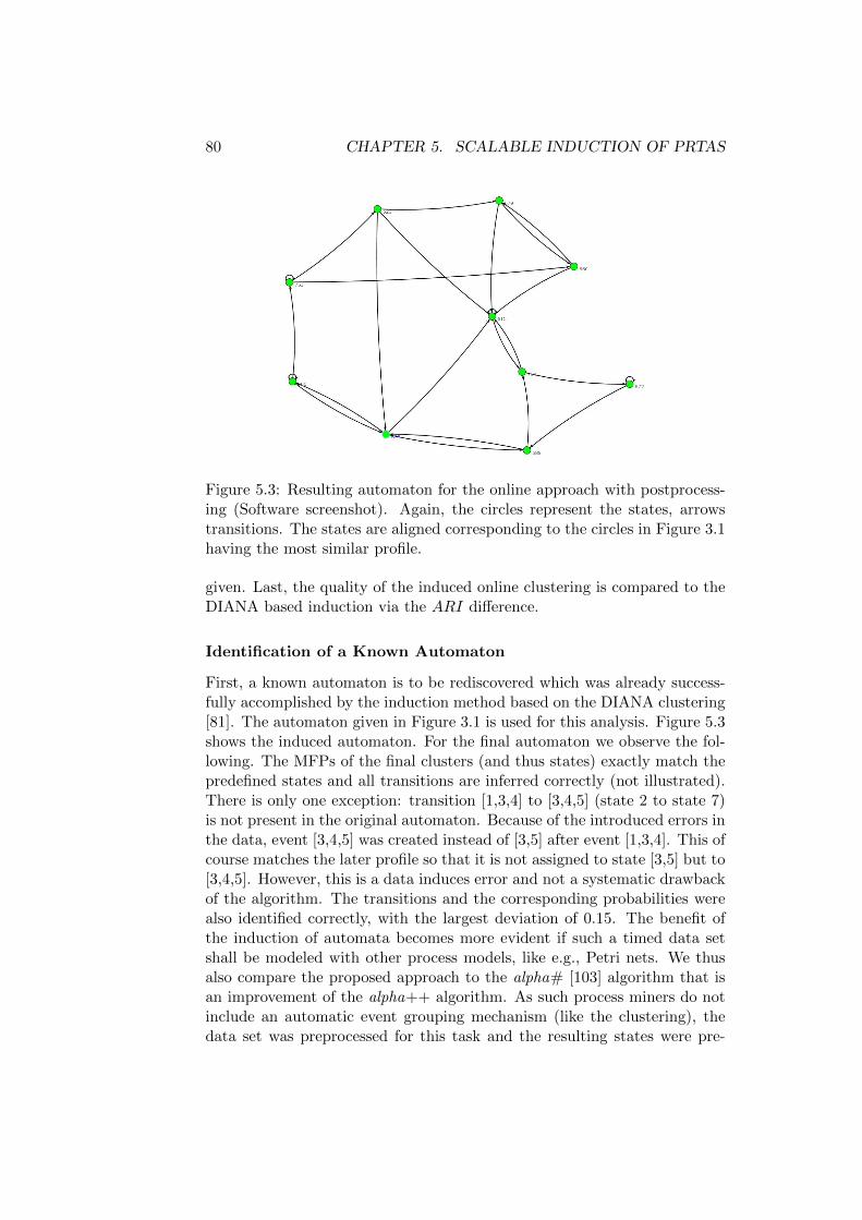
80 CHAPTER 5. SCALABLE INDUCTION OF PRTAS
Figure 5.3: Resulting automaton for the online approach with postprocess-ing (Software screenshot). Again, the circles represent the states, arrowstransitions. The states are aligned corresponding to the circles in Figure 3.1having the most similar profile.
given. Last, the quality of the induced online clustering is compared to theDIANA based induction via the ARI difference.
Identification of a Known Automaton
First, a known automaton is to be rediscovered which was already success-fully accomplished by the induction method based on the DIANA clustering[81]. The automaton given in Figure 3.1 is used for this analysis. Figure 5.3shows the induced automaton. For the final automaton we observe the fol-lowing. The MFPs of the final clusters (and thus states) exactly match thepredefined states and all transitions are inferred correctly (not illustrated).There is only one exception: transition [1,3,4] to [3,4,5] (state 2 to state 7)is not present in the original automaton. Because of the introduced errors inthe data, event [3,4,5] was created instead of [3,5] after event [1,3,4]. This ofcourse matches the later profile so that it is not assigned to state [3,5] but to[3,4,5]. However, this is a data induces error and not a systematic drawbackof the algorithm. The transitions and the corresponding probabilities werealso identified correctly, with the largest deviation of 0.15. The benefit ofthe induction of automata becomes more evident if such a timed data setshall be modeled with other process models, like e.g., Petri nets. We thusalso compare the proposed approach to the alpha# [103] algorithm that isan improvement of the alpha++ algorithm. As such process miners do notinclude an automatic event grouping mechanism (like the clustering), thedata set was preprocessed for this task and the resulting states were pre-

5.2. EXPERIMENTS 81
Figure 5.4: Resulting Petri nets using alpha++ (B) and alpha# (C) com-pared to the given synthetic model (A), cf. Figure 3.1.
sented to the algorithm. Thus only the states’ relations and not the statesthemselves had to be found. Figure 5.4B and C show the resulting modelsfor the alpha++ and alpha# algorithm. Note that there, the squares arecalled states while the circles are called places. Moreover, Figure 5.4 C alsoincludes hidden states (white squares) to model e.g., switches. Althoughthe overall structure is identified correctly, there are states in both modelsthat do not correctly reflect the data: e.g., alpha++ fails to correctly inferthe relations of state 2 and 5 while alpha# does indeed better, but alsomisses transitions (e.g., from state 7 to state 4). This is due to the fact thatPetri nets have to satisfy constraints regarding liveliness, reachability andboundness. Therefore, for more complex temporal relationships as given inthe current problem setting, such models are not appropriate.
Parameter Dependence
This section analyzes some structural properties of the automaton for theparameters: minimum support and number of input instances. Figure 5.5shows two important properties of the resulting automaton when varyingthe minimum support θ in the clustering step. First, for a higher θ, thenumber of states decreases. This is the result of the decreasing size of the

82 CHAPTER 5. SCALABLE INDUCTION OF PRTAS
Figure 5.5: Recovery ratio (RR) for states 1, 3, 7 and 10 of the syntheticautomaton.
Figure 5.6: Runtime and final number of states with increasing data setsizes for the synthetic data sets.

5.2. EXPERIMENTS 83
MFP found in the clusters. As there are exceptions in the data, not everyconcept of the state is present in each event. Thus the frequencies of largepatterns decrease and only small MFPs are found. These small MFPs areof course better to cover than large ones even if the cluster size is largeand thus less clusters are necessary for a good coverage ratio. The numberof transitions (not shown) decreases simultaneously, because the number ofstates is also decreasing. Second, there are states that are identified betterthan others. The lines in Figure 5.5 exemplarily give the RR for the states1,3,7 and 10. State 7 is very difficult to recover due to two reasons: a)it is very similar to state 3, thus a separation is not always possible andb) it only has one incoming transition with a small probability. Therefore,this event is not often present in the data and can also be regarded as anexception of state 3. Additionally, state 10 is harder to find with increasingminimum support. Again, this is due to the similarity to state 5. For theremaining states a quite stable recovery ratio is observed, but the detectionrate decreases with increasing minimum support, due to the smaller MFPs.Another important parameter is the number of input histories, and how thisnumber affects the runtime of the approach. This is shown in Figure 5.6once for the presented online approach as well as for the approach based onDIANA clustering. We tested our approach on up to 40,000 histories, whichcorresponds to a data set having 220,000 events (because each history has5.5 events on average). Note that the traditional approach (using DIANAclustering) can handle only 2000 histories of the same length due to itshigh complexity. The runtime of the online approach is divided into threeseparate runtimes: the time that is needed for the PTA construction, thetime for the clustering and the time of the postprocessing step. For theDIANA approach only the time for the clustering is given, because thePTA construction time is the same and moreover, no postprocessing step isconducted. As expected, the runtime increases for larger data sets for bothapproaches. However, the runtime difference for large data sets between theonline approach and DIANA is tremendous. The clustering part of the onlineapproach now is the fastest step. Considering the number of final states,both methods result in too many states. This can be explained by exceptionsin the data. As more data is available, rare events, i.e. events that stronglydiffer from their original states, are observed more often. Thus, they arealso clustered in a separate group. However, the number of final states forboth methods converges, but altogether the online approach identifies fewerstates than the DIANA based induction. This indicates that it may be ableto better find the main information in a data set.
Stability Analysis
In this section the stability of the online approach is presented. Figure 5.7shows the result of a bootstrap analysis. Figure 5.7b gives the difference

84 CHAPTER 5. SCALABLE INDUCTION OF PRTAS
●
●
●
●●●●●●
●
●●●●
● ●●
●
●●
●
●
●
●●●
●●
●●●
●
●
●●●●
●
●●●●
●
●●●●●
●●●
●
●
●●●●●●● ●●
●
●●
●
●●●
●
●●●●
●
●
●
●
●
●
●
●
●
●
●
●
●
●●
●
●
●
●●●●●●
●●
●●
●
●
●
●●●
●
●●●
●
●●●
●●
●●●●●●
●
●
●
●
●
●●●
●●
●
●●
●●●
●●
●
●
●
● ●●
●
●
●
●●
●●
●
●
●●
●
●
●
●
●
●
●●●●●●●●
●●
●●
●
●●●
●
●
●●
●
●
●
●
●
●●●
●
●●
●●●
●
●●●
●
●●●●●●●●●●●●
●●
●
●
●●●
●
●●
●
●●●
●
●●
●●
●●●
●
●●
●
●●●●●
●
●●●●
●
●
●
●●
●●●●●●
●●●
●
●●●●●●
●
●
●●
●
●●
●
●
●
●
●●
●●
●
●
●
●
●●
●●●●●
●●●
●
●●
●
●●●●
●
●
●●●●●
●
●
●
●●●
●
●
●●●
● ●●●●●
●
●
●●
●●
●
●
●
●
●●
●●●●●
●
●●
●
● ●
●●
●
●●
●
●
●●
−8
−6
−4
−2
02
4
sampling with replacementpercentage sampled
diffe
renc
e in
sta
tes
0 10 20 30 40 50 60 70 80 90 100
(a) Boxplot: Difference of states DIANA
●●●●●●●●●●●●●●
●●●●●●●
●●
●●●●●●
●
●●●●
●●●
●●
●
●●●●●
●
●
●
●●
●
●●
●●
●● ●●●
●
●●●●●
●
●
●
●●
●●●●
●
●
●
●●●●●●●
●●
●●●
●
●●●●●●●●●●●●●●●
●
●
●
●●●●●
●
●●●●●●
●
●● ●●●
●
●
●
●
●
●
●● ●
●
●
●
●●●●●●●
●
●●●●●
●
●●●●●
●
●●●●●
●
●●
●
●●
●
●●
●●
●
●
●●●
●
●●●
●●●●●●●
●●●
●●●
●●●●
●
●
●●●
●
●
●●●
●
●●●●
●
●
●
●
●●●●
●●●●
●
●
●
●
●
●●
●
●●●
●●●●
●
●●
●
●
●
●●●
●
●●●●●●●●●●●
●●
●
●
●●
●
●●●●●●●●●●●●●●●
●
●●
●
●
●●●●
●
●
●
●
●
●
●●●●●●●●●●
●
●●
●●●●●●●
●
●
●
●
●●
●
●
●
●●●●●● ●●
●
●
●
●
●●
●
●●●●●●●●
●
●
●
●
●●
●
●●●●●●
●
●●●●●
●
●
●
●●●●●●●
−8
−6
−4
−2
02
4
sampling with replacementpercentage sampled
diffe
renc
e in
sta
tes
0 10 20 30 40 50 60 70 80 90 100
(b) Boxplot: Difference of states online
0.0
0.5
1.0
1.5
2.0
2.5
sampling with replacementpercentage sampled
eucl
idea
n di
stan
ce to
orig
inal
sta
tes
0 10 20 30 40 50 60 70 80 90 100
(c) Loss of learned states DIANA
0.0
0.5
1.0
1.5
2.0
2.5
3.0
sampling with replacementpercentage sampled
eucl
idea
n di
stan
ce to
orig
inal
sta
tes
0 10 20 30 40 50 60 70 80 90 100
(d) Loss of learned states online
F−Measure Transition Learning
F−Measure
Fre
quen
cy
0.6 0.7 0.8 0.9 1.0
020
4060
8010
0
(e) F-Measure of transitions DIANA
F−Measure
Fre
quen
cy
0.6 0.7 0.8 0.9 1.0
020
4060
8010
012
014
0
(f) F-Measure of transitions online
Figure 5.7: Bootstrap analysis: Structural dependencies for the DIANAbased clustering compared to the online approach, (DIANA c = 0.3, onlineθ = 0.5)

5.2. EXPERIMENTS 85
between the number of learned and expected states (10) on the 10 syntheticdata sets of 100 histories. The higher the sample size, the more likely thecorrect number of states is found. Although the average number of states is10 for a sample size above 75%, there are exceptions that find 11 or 9 states.A smaller number of states can be due to a missing example in the data, ahigher number of final states may be due to exceptions in the data that areplaced in a separate cluster. Figure 5.7d shows the average distance betweenthe learned states and the most similar states of the original automaton. Forsmall sample sizes, this distance can be large, but it rapidly decreases forlarger data sets. Figure 5.7f shows how often the transitions were identifiedcorrectly. For this figure, only automata that induced the correct numberof states were regarded: DIANA found the correct number of states in 318cases, while the proposed online approach successfully found the 10 statesin 369 cases. Each learned state is mapped onto its most similar originalstate. Then, the corresponding transition between the learned states can bevalidated whether they are correct or wrong and thus whether true or falsepositives/negatives are identified. The figure shows that in most cases thetransitions are identified correctly. Precision and recall (not displayed) aremostly above 80%. However, recall is the limiting factor as it has a worsedistribution than precision. This indicates that the found transitions arecorrect, however some transitions are missing. Comparing these results tothe DIANA based induction (cf. Figure 5.7a - 5.7e bottom) the presentedonline approach outperforms it in each category: The number of inferredstates is closer to the original (cf. Figure 5.7b bottom: DIANA overestimatesthe number of states) and has a smaller variance. Moreover, the distance ofthe states to their closest original is smaller (cf. Figure 5.7d bottom) whilefewer data samples are necessary to reach this quality (for sample sizes of20% the final state distance is already achieved). Thus, also the transitionsare learned better (cf. Figure 5.7e bottom: the distribution of the F-Measureof DIANA is shifted to the left).
Quality of the Online Approach
Another parameter to evaluate the quality of the online clustering approachis the resulting ARI. The zoo data set is used for this task because italso has a class label assigned to each instance. To validate exclusivelythe clustering, only the resulting clustering for the nodes of the PTA isinspected, and not the automaton itself. Table 5.1 shows the resulting ARIfor a DIANA based induction and the online approach. Note that the resultsfor the different parameters (c = distance cutoff and θ = minimum support)cannot be compared directly because they have a different influence on theclustering. However, the results show that a similar quality can be achievedby the online approach. Its best ARI of 0.84 reaches the best value of theDIANA approach. Moreover, the online approach achieves at least an ARI

86 CHAPTER 5. SCALABLE INDUCTION OF PRTAS
D c = .1 .2 .3 .4 .5 .6 .7 .8 .9 1.00.17 0.35 0.47 0.49 0.58 0.86 0.80 0.48 0.22 0.0
O θ = .1 .2 .3 .4 .5 .6 .7 .8 .9 1.00.40 0.36 0.56 0.50 0.60 0.58 0.77 0.84 0.63 0.7
Table 5.1: ARI for the DIANA clustering (D) and online clustering (O)depending on their primary parameter for the zoo data set
of 0.36, which is better than the DIANA clustering. Finally, these numbersshow that although the online approach induces fewer clusters than DIANA,these clusters also make sense and thus the clustering informative.
5.2.2 Performance of the Online Approach on a Real WorldExample
In this section, examples of how to use such an automaton on real worlddata are given. Moreover, the runtime and structural dependence on thenumber of input histories for these data sets are presented.
Yeast Gene Expression
A first experiment addresses the knowledge one can gain from such a typeof automaton. Figure 5.8 presents the automaton (with the correspondingprofile for each state) that was induced for the yeast gene expression dataset. The first important point that can be observed from this figure is that itshows a cyclic structure, which is known to be the cell cycle. The automatonis thus capable of correctly identifying the stages of life in a population or ofindividuals. Second, each state is annotated with a specific gene expressionprofile that shows the current metabolism of the cell. Following the cycle,one can easily observe which genes are activated after another and whichgenes are co-expressed. Third, a resting phase between state 1 and 2 isidentified via the delay guard (φ = [1, 2]) on the corresponding transition.This shows that the cell can rest between two cell dividing phases. Thereis only one state that could be better separated from the other state: theprofile of state 6 is not as specific as the others. This is due to the fact thatthere is one instance included that should occur as a separate state beforestate 6. This also leads to state 7 being a loop structure. However, thisassignment is due to the initial variability in the clusters.
Hepatitis Data
This section presents the results of the online approach on the Hepatitis dataset. To test the performance, differently sized data sets from the original onewere derived. Compared to the synthetic data set, the Hepatitis data set is

5.2. EXPERIMENTS 87
Figure 5.8: Automaton for the yeast data set. For each resulting state (cir-cle) the corresponding profile of the state is given. The profile is illustratedby the boxes next to each state where each gene’s expression values is indi-cated by a grey-scaled square. The expression profile for gene i is given bythe ith square, beginning from the left. The darker, the higher is the gene’sexpression value.
a difficult one, because it is very dense and has more attributes. Moreover,the histories are long and the resulting PTA is also very large, because onlyfew histories have the same prefix. Figure 5.9 gives the runtimes for theHepatitis data set for the presented approach. (The results for DIANA arenot displayed as only the smallest data set could be processed.) Even forthe smallest number of histories (50), DIANA needs longer (218 s) than theonline approach (173 s) for the largest data set (1236 histories). This iscaused by the huge number of states on which DIANA operates: 2465 statesin the PTA must be clustered for the smallest data set. Although this isstill feasible, DIANA runs out of memory for the larger Hepatitis data sets.But also for the online approach, the runtimes are higher. Note that the1236 histories lead to a PTA with 51,699 states. However, comparing thenumber final states (188) of the online approach for 1236 histories to theDIANA clustering with only 50 histories (338 final states), again a morecompact representation can be inferred. Another interesting aspect of theonline approach is the distribution of the number of MFPs per final clusterand their lengths. Figure 5.10 shows how these distributions vary for moreand more input histories. Note that for a better visualization not every dataset size result is displayed. Figure 5.10 shows that the majority of clusters isrepresented by long MFPs: mostly more than two attributes contribute to

88 CHAPTER 5. SCALABLE INDUCTION OF PRTAS
Figure 5.9: Runtime and number of states of the online approach for theHepatitis data sets.
a MFP. This distribution is quite constant over the different data set sizes.Next to that, in most cases, only few representatives are induced by theclustering (cf. the lines in Figure 5.10). Moreover, the more histories areused for the creation of the automaton, the fewer MFPs are present in theclustering. This indicates that instances sharing large patterns are groupedtogether, and thus homogeneous states are found.
5.3 Conclusion
We presented a scalable method of learning probabilistic real-time automata(PRTAs), a new type of model that captures the dynamics of multi-dimensionalevent logs. It is based on a state merging process, which is the current stateof the art in automaton induction. As the state merging is guided by aclustering in our approach, the clustering procedure needs to scale well tomake the overall approach scalable. Therefore, we employ an online clus-tering procedure as a plug-in that is based on maximum frequent patterns(MFPs) to decide where to assign states. The approach is compared to in-duction variant using DIANA clustering. The proposed online method isfaster than the one based on DIANA, computes a more compact automatonstructure and also works for significantly larger data sets. In future work,

5.3. CONCLUSION 89
Figure 5.10: Distribution of the length of MFPS (number of items in apattern) and number of MFPs per cluster (seconday axis).
we would like to improve the creation of the PTA, which is currently anotherbottleneck in the induction of automata.

90 CHAPTER 5. SCALABLE INDUCTION OF PRTAS

Chapter 6
Augemented Itemset Trees
Data streams are ubiquitous today due to the surge of data produced bysensor networks, social networks and high throughput methods in biologyand medicine, to name just a few areas of interest. For streams of binarydata, one of the most basic and fundamental data types, online versionsof classical data mining methods for itemset mining have been developed[17, 91]. These methods allow for mining patterns in sliding windows or forthe full amount of data via, e.g. data buckets. While the sliding windowsapproach addresses the task of concept drift and does not provide exactsolutions over the complete data stream so far, the approach based on buck-ets faces a number of problems. First, it is not feasible if main memory islimited (below the expected data set size) or I/O operations are expensive.Second, it is not incremental in the strict sense of the word, with updatesusing newly observed instances. Third, the detection of change is not easy,because either it is delayed due to large buckets, or the mining process isslowed down due to small buckets for which the pattern extraction step mustbe repeated frequently. In this chapter, we consider the incremental case ofmaximum frequent pattern (MFP) mining where the set of solutions is avail-able after each instance without having to store previous instances explicitly.This can also be seen as a step towards a batch-incremental algorithm foronline MFP mining, in which the solution set is updated after a batch ofinstances. Algorithms for online MFP mining can be useful for various pur-poses, e.g. for building fast incremental clustering algorithms on 0/1 datawith maximal frequent itemsets as cluster representatives, in analogy to agraph clustering approach that was proposed recently [83]. More specifically,we introduce the Augmented Itemset Tree (AIST), a new data structure thathelps mining maximum frequent patterns incrementally. It is a mixture ofitemset trees (IST) [39] and FP-Trees [41], combining advantages of both:a canonical ordering of patterns and a connection between patterns sharingthe same items. The first idea is that search starts with maximal patterncandidates P , which is opposite to traditional search strategies, beginning
91

92 CHAPTER 6. AUGEMENTED ITEMSET TREES
with 1-itemsets and iteratively increasing the length of the candidate pat-terns. But if the maximal patterns are expected to be large, i.e. consist ofmore than half of all possible items, a top-down search strategy is more ap-propriate: the number of candidates of the pattern space in each candidatelevel is symmetric
(nk
)=(n
n−k)
(e.g. |P1| = |Pn−1|). If maximal patternsare large, then fewer candidates are evaluated, when starting with maximalpatterns instead of beginning with patterns of size one. A second strategy isthat the set of candidates is composed of all former MFPs and the patternsof the new instance. These patterns serve as a starting point for the searchof the new maximal frequent patterns, which prevents unnecessary patternsfrom evaluation.
6.1 Related Work
Frequent pattern mining is a well-studied problem and many improvementshave been achieved since its introduction [1]. In this part of the thesis, weconsider the case that the set of maximal frequent patterns is to be identifiedin an incremental manner. This also includes that instances are presented tothe algorithm one by one, i.e. no instances are kept in memory and only onedata scan is allowed. In the following, we discuss various solutions that wereproposed for an online setting. The earliest approach, Apriori [16], relieson a candidate generation and test procedure involving several scans over adatabase. This is of course not possible for the incremental case, becausethe final size of the data set is not known in advance. However, there areadaptations that are based on Apriori via piece-wise mining of bags of in-stances or using a graph structure to identify the positive or negative borderin modified databases [90, 91]. Han et al. [41] developed an algorithm thatuses a tree-like structure for the mining process, the so-called frequent pat-tern tree (FP-tree). It stores the content of the given data set by scanningthe database twice and creating a pattern tree, where the items are includedcorresponding to their frequency. This property forces the second databasescan. Next, the FP-tree uses the pattern growth technique to derive fre-quent patterns. Each path of the tree stores items in decreasing frequency.A main disadvantage of such a tree structure for the incremental case is thatthe frequency of the patterns is not known in advance. This implies thatthe tree must always be restructured [55] when the frequency of itemsetschanges. If a reordering occurs frequently, such an algorithm will be lessefficient for incremental data. An approach to use FP-trees in an incremen-tal setting was proposed [17], but does not reach the performance of othermethods [55]. Another group of algorithms mines frequent patterns using adata structure similar to itemset trees. An efficient algorithm, CanTree, thatincrementally mines frequent itemsets in a finite database was proposed re-
6.2. PROBLEM STATEMENT 93
cently [55]. It outperforms FP-based algorithms and also explains why a treewith a given canonical ordering is to be preferred in an incremental setting:No reorganization of the data structure is necessary. However, CanTree isnot designed to keep track of the current maximal frequent itemsets, whichis the problem addressed here. Instead, the mining step is only conductedafter the database scan is finished. In a possibly infinite online setting, thismay never be the case. Therefore, a modified version of the CanTree hasbeen developed that is able to keep track of the current maximal frequentpatterns. We apply a technique similar to previous work that describes howto mine frequent closed patterns for data streams [54] based on the currentclosed sets and a new instance. However, this theoretical work neither pro-poses an efficient data structure nor provides an experimental evaluation.Approaches to mine frequent patterns incrementally, but in a different set-ting, were also proposed in recent years (Moment [18], SWIM [63], DISC [20],FLAME [32], DSM-MFI [58] and CP-tree [53]). Moment, SWIM, DSM-MFIand DISC find frequent patterns in a sliding window over data streams anduse instances for later evaluations. FLAME and CP-tree identify approxi-mate patterns. Moment uses the closed itemset tree (CET) data structurethat represents the border of frequent patterns in its nodes. Four nodetypes differentiate between frequent patterns and promising patterns, i.e.patterns that are not yet frequent but may become frequent. Although itsnode frequency update strategy is very efficient, it needs to keep track ofthe current transactions of the sliding window. Otherwise it is not able toupdate relevant node counts for patterns that were not yet incorporatedinto the CET. The same argument applies to the SWIM algorithm [63] andthe DISC strategy [20]. For unrecorded patterns that may become frequent,additional passes over the current window are necessary. Similarly, MFPMining based on the SG-Tree [59] also stores the itemsets that were ob-served but uses the same top down strategy to find the MFPs. In contrastto these approaches, the AIST works for the instance-incremental setting,where each instance is only observed once, patterns over the complete datastream are of interest and an immediate response is necessary.
In the remaining of this chapter, we describe the problem setting andthe data structure to support the solution. Subsequently, each of the mainsteps of the algorithm is explained in detail.
6.2 Problem statement
Let D be a data stream of instances xi, each instance being a vector of lbinary attributes (xij ∈ {0, 1}). We assume that one instance is observedafter the other, starting with x1, x2, .... The goal is to find all MFPs for thedata stream part Dm = 〈x1, . . . , xm〉, in other words, for each new instancexm, the updated set of maximal frequent patterns. In the following, we

94 CHAPTER 6. AUGEMENTED ITEMSET TREES
will use the itemset notation for patterns and instances: Each instance xi istransformed into an ordered itemset Ii = ι1, . . . , ιz, where item ιj is includedin the itemset if xij = 1. This turns a data set into a multiset of itemsets. Asusual, the support of an itemset Ii, support(Ii), is defined as the percentage|Y |/|Di| of itemsets Y in Di such that Ii ⊆ Yj . Informally, this is the relativefrequency of instances that include the itemset Ii. All patterns exceedingthe minimum support constraint (minsup constraint) θ ∈ [0, 1] are frequent(F ), infrequent otherwise (F ). The more general relation p ≺ q implies anordering upon patterns p and q [1]. Pattern p is more general than patternq iff p occurs whenever q occurs, i.e. all items of p are also included in qbut not vice versa. For the pattern domain of items, p ≺ q is defined by setinclusion p ⊂ q. Pattern p is called subpattern of q, while q is a superpatternof p. Let the set of all patterns p that are more general than q be denotedby G:
G(q) = {p | p ≺ q} (6.1)
Accordingly, S(q) comprises all patterns that are more specific than g. Apattern p is maximal if there is no other pattern q that is frequent and asuperpattern of p.
p ∈MFP ↔ p ∈ F ∧ ¬∃q : q ∈ F ∧ p ≺ q (6.2)
If a pattern p is a subset of an instance Ii, we say that the patterns coversthe instance, or alternatively, occurs in the instance. The final problem canhence be expressed as: For a data set of instances I, successively update theset of MFPs with respect to a given minimum support threshold θ.
6.3 Proof of main concept
The basic assumption of the approach is that the updated MFPs are de-termined by the MFPs known up to that point and subsets of the newinstance. Similar approches also make use of this property [54, 75] To provethat this is sufficient, we first summarize how the set of updated frequentpatterns is identified and then, how the corresponding MFPs can be derived.Therefore, we divide the set of all patterns P into four subsets P1, . . . , P4
that define whether a pattern is frequent (F ) and covered (C) by a newinstance (cf. Figure 6.3, right): P1 = {p|p ∈ F ∩ C}, P2 = {p|p ∈ F ∩ C},P3 = {p|p ∈ F ∩ C} and P4 = {p|p ∈ F ∩ C}.
Theorem The set of (M)FP (F ′) including a new instance, is a subsetof the patterns of (1) all former (M)FP (F ) and (2) all patterns occurringin the new instance (C).
Proof Start of induction, A(1), regarding the first instanceThere are no frequent patterns in an empty set: F = ∅, F = ∅. The set
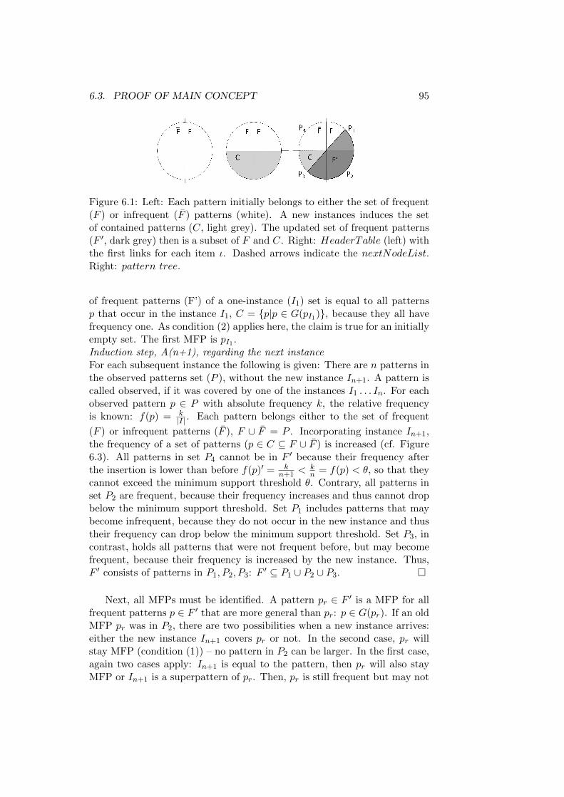
6.3. PROOF OF MAIN CONCEPT 95
Figure 6.1: Left: Each pattern initially belongs to either the set of frequent(F ) or infrequent (F ) patterns (white). A new instances induces the setof contained patterns (C, light grey). The updated set of frequent patterns(F ′, dark grey) then is a subset of F and C. Right: HeaderTable (left) withthe first links for each item ι. Dashed arrows indicate the nextNodeList.Right: pattern tree.
of frequent patterns (F’) of a one-instance (I1) set is equal to all patternsp that occur in the instance I1, C = {p|p ∈ G(pI1)}, because they all havefrequency one. As condition (2) applies here, the claim is true for an initiallyempty set. The first MFP is pI1 .Induction step, A(n+1), regarding the next instanceFor each subsequent instance the following is given: There are n patterns inthe observed patterns set (P ), without the new instance In+1. A pattern iscalled observed, if it was covered by one of the instances I1 . . . In. For eachobserved pattern p ∈ P with absolute frequency k, the relative frequencyis known: f(p) = k
|I| . Each pattern belongs either to the set of frequent
(F ) or infrequent patterns (F ), F ∪ F = P . Incorporating instance In+1,the frequency of a set of patterns (p ∈ C ⊆ F ∪ F ) is increased (cf. Figure6.3). All patterns in set P4 cannot be in F ′ because their frequency afterthe insertion is lower than before f(p)′ = k
n+1 <kn = f(p) < θ, so that they
cannot exceed the minimum support threshold θ. Contrary, all patterns inset P2 are frequent, because their frequency increases and thus cannot dropbelow the minimum support threshold. Set P1 includes patterns that maybecome infrequent, because they do not occur in the new instance and thustheir frequency can drop below the minimum support threshold. Set P3, incontrast, holds all patterns that were not frequent before, but may becomefrequent, because their frequency is increased by the new instance. Thus,F ′ consists of patterns in P1, P2, P3: F ′ ⊆ P1 ∪ P2 ∪ P3. �
Next, all MFPs must be identified. A pattern pr ∈ F ′ is a MFP for allfrequent patterns p ∈ F ′ that are more general than pr: p ∈ G(pr). If an oldMFP pr was in P2, there are two possibilities when a new instance arrives:either the new instance In+1 covers pr or not. In the second case, pr willstay MFP (condition (1)) – no pattern in P2 can be larger. In the first case,again two cases apply: In+1 is equal to the pattern, then pr will also stayMFP or In+1 is a superpattern of pr. Then, pr is still frequent but may not

96 CHAPTER 6. AUGEMENTED ITEMSET TREES
become maximal, because a superpattern of pr can become frequent. Thismay be true for all patterns p∗r ’between’ pr and In+1: In+1 � p∗r ≺ pr. Forthis situation condition (2) applies, the set of the new MFP is derived fromthe new instance In+1. To avoid that, F ′ is inspected whether a pattern isnot maximal anymore. If pr ∈ P1, it may become infrequent, but some pmay nevertheless be frequent. In this case, following condition (1) a depthfirst search (DFS) is conducted that tests each subset of pr until a new MFPp′r is found: p′r ∈ G(pr). Finally, only patterns p ∈ P3 remain that are nowfrequent, where no MFP was identified yet. As only patterns that occurredin the new instance p ∈ G(pIn+1) may become frequent (condition (2)), thenew MFP is also a subpattern of pIn+1 and is identified via DFS.
6.4 Main idea of the used data structure
The basic assumption of the approach is that the updated MFPs are deter-mined by the MFPs known up to that point and patterns covered by thenew instance. The proof is ommitted here due to space constraints but issimilarily shown for other approaches [54, 75]. Intuitively, it is clear that nonew MFP can emerge if it was neither in the old set of MFPs nor in the newinstance. The data structure that makes use of this property is called Aug-mented Itemset Tree (AIST). Figure 6.2 shows the main idea of an AIST:It consists of a pattern tree (right part) and a headerTable (left part). Itis a mixture of FP-trees [41] and ISTs [39] and designed to fulfill two mainrequirements: (1) quick look-ups for patterns and (2) quick subset checks.Each node represents a pattern with the last item being ιj , where the iden-tifier j of a node corresponds to item ιj . The first requirement is solved byusing an itemset-tree like structure: nodes follow a canonical ordering in thetree (top-down arrows), i.e., the parent of a node n has a smaller identifierthan n itself. To cope with the second constraint, each node is linked toanother one with the same identifier but of smaller or equal tree level. Thissets up a list (nextNodeList) that connects all patterns sharing item ιj ,ordered by decreasing tree level. This idea was already used in FP-trees andreduces unnecessary subset checks. A headerTable stores the first link foreach item ιj . Although it is a mixture of two known data types, it is stilldifferent from them. FP-trees are not canonically ordered and ISTs do notinclude cross-links between patterns sharing items. The combination of thetwo concepts enables efficient mining of MFPs in an online setting.
6.5 Definition of the AIST
The purpose of the AIST is to keep track of all relevant patterns, i.e., MFPsor former MFPs. Since the AIST is not forced to store all possible (subset)patterns, it saves a lot of space and is also computationally more efficient.
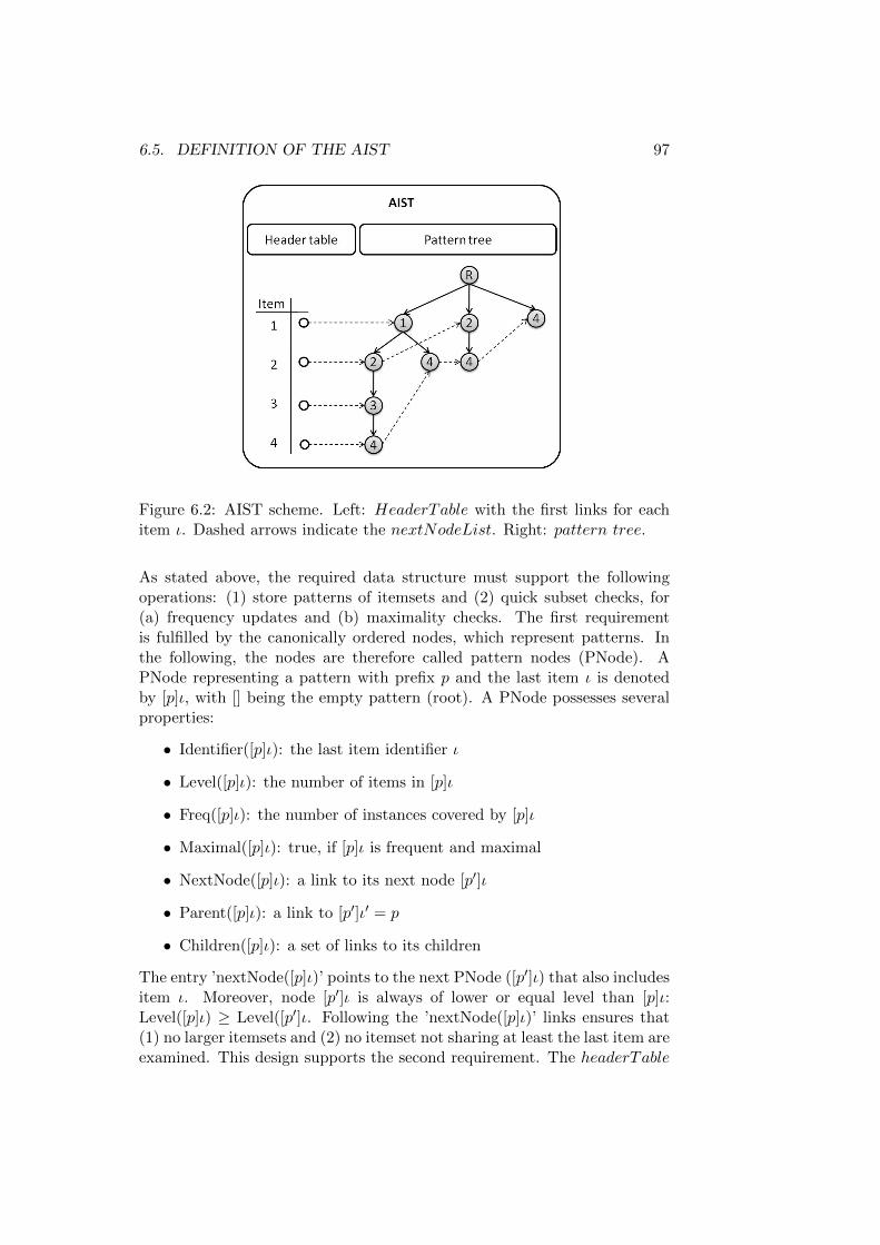
6.5. DEFINITION OF THE AIST 97
Figure 6.2: AIST scheme. Left: HeaderTable with the first links for eachitem ι. Dashed arrows indicate the nextNodeList. Right: pattern tree.
As stated above, the required data structure must support the followingoperations: (1) store patterns of itemsets and (2) quick subset checks, for(a) frequency updates and (b) maximality checks. The first requirementis fulfilled by the canonically ordered nodes, which represent patterns. Inthe following, the nodes are therefore called pattern nodes (PNode). APNode representing a pattern with prefix p and the last item ι is denotedby [p]ι, with [] being the empty pattern (root). A PNode possesses severalproperties:
• Identifier([p]ι): the last item identifier ι
• Level([p]ι): the number of items in [p]ι
• Freq([p]ι): the number of instances covered by [p]ι
• Maximal([p]ι): true, if [p]ι is frequent and maximal
• NextNode([p]ι): a link to its next node [p′]ι
• Parent([p]ι): a link to [p′]ι′ = p
• Children([p]ι): a set of links to its children
The entry ’nextNode([p]ι)’ points to the next PNode ([p′]ι) that also includesitem ι. Moreover, node [p′]ι is always of lower or equal level than [p]ι:Level([p]ι) ≥ Level([p′]ι. Following the ’nextNode([p]ι)’ links ensures that(1) no larger itemsets and (2) no itemset not sharing at least the last item areexamined. This design supports the second requirement. The headerTable

98 CHAPTER 6. AUGEMENTED ITEMSET TREES
stores the initial pointer for an identifier’s nextNodeList, i.e. the PNodewith the highest level containing identifier ι:
H(ι) = argmax[p]ι(level([p]ι))
. The pattern tree of an AIST can be defined recursively: it is empty orit consists of a PNode r and an empty or nonempty list of pattern treest1, . . . , tn (list of children). Each PNode ri is connected to r by an edge(parent link) and ri’s identifier is strictly greater than r’s. The root ofthe AIST is the PNode of level 0, with an empty identifier, thus being theempty pattern. Each PNode represents the pattern that consists of its ownidentifier and all identifiers of its parents.
6.5.1 InsertPattern
Roughly speaking, the algorithm works as follows (cf. Algorithm 8): Foreach instance, the maximal occurring pattern (namely the pattern that in-cludes all items from the instance [Algorithm 8 lines 3 to 5 ] ) is insertedinto the AIST and if it is frequent, added to the set of MFPs (Algorithm8 line 11). If not, it serves as a candidate for the MFP search (cf. Section6.5.2) which is conducted subsequently. Last, all former MFPs are inspectedwhether they are still frequent and, if not, they again serve as candidates.This implies that subsequently the set of MFPs is updated. As the insertionof patterns is a major step in this procedure, it will now be presented indetail. Each item ι of the occurring pattern P is inserted in the AIST oneby one, canonically ordered. Inserting means that either a new node [p]ι iscreated, if there is no path [p] with child ι, or that the frequency of [p]ι is in-creased by freq. Beginning at the root, it is checked whether there alreadyexists an item in the children’s list of the current node [p] with identifierι. If this is not the case, a new child [p]ι is created with the given item ιand prefix [p]. Subsequently, the link nextNode([p]ι) is set, i.e., the node[p]ι is inserted into the nextNodeList of item ι. Then, the frequency of thepattern is increased by the given frequency count (freq, usually one) plusthe frequency counts of all supersets (retrieved by method setNextNode).Subsequently, all subset frequencies are also increased by freq, in order topreserve consistency. This is done in function UpdateMoreGeneralCounts.If the current pattern pi is a MFP, it is added to the set containing all MFPs.
Example: Let the AIST of Figure 6.2 be given where pattern {1, 3, 4}is observed. As all items are subsequently inserted into the tree, for itemι = 1 the root (which is the current node) is examined whether it has achild ι = 1. This is true, the current node is set to []1 and its frequency isincreased. The next item is ι = 3. Because []1 has no child [1]3, this nodeis created and added (with frequency 1) to the children list of []1. Then,

6.5. DEFINITION OF THE AIST 99
Algorithm 8 InsertPattern
Require: pattern (canonically ordered) P , int freq1: active = AIST.root2: for each item ι ∈ P do3: if !( active has child [p]ι) then4: create [p]ι and add [p]ι to active’s children5: SetNextNode([p]ι)6: end if7: node = child [p]ι of active8: node.increaseFrequency(freq)9: UpdateMoreGeneralCounts(node, freq)
10: if isMFP(node) then11: addToMFPs(node)12: end if13: active = node14: end for
it is inserted in the nextNodeList of ι = 3, which is after [1, 2]3. It hasno successor, because no other pattern containing item 3 is currently storedin the AIST. During this insertion, the exclusive counts of all supersets arederived (cf. the paragraph on SetNextNode), which is then added to thefrequency of [1]3. Next, item ι = 4 (level 3) is inserted in the same manner.Its place in the nextNodeList of ι = 4 is after [1, 2, 3]4 (level 4) and before[1]4 (level 2). Finally, the AIST has an additional path [1, 3]4.
SetNextNode
The method SetNextNode (Algorithm 9) finds the correct predecessor andsuccessor for a PNode [p]ι in the nextNodeList. Additionally, the fre-quencies of all supersets are summed up and finally added to [p]ι’s fre-quency. Starting at the headerTable’s entry for item ι, all nextNode linksare followed until the first PNode [p′]ι with Level([p′]ι) ≤ Level([p]ι) isreached. Then the pointer of NextNode([p]ι) is set to [p′]ι and the pointerofNextNode([p′]ι’s predecessor) to [p]ι. While following theNextNodeList,the visited PNodes [p′′]ι are explored whether they are supersets of [p]ι andprovide a frequency strictly greater than the elements [p′]ι that are alreadyin the set SsP . If this is the case, they are added to the set of [p]ι’s su-persets (SsP ). (cf. Algorithm 10). When the final position [p∗]ι of [p]ι inthe NextNodeList is determined, SsP holds all supersets of [p]ι and theirexclusive frequencies, respectively. This means that the count of all occur-rences of the pattern has the count of all occurrences of their superpatternssubstracted. Thus the counts of subpatterns are not repeatedly counted.The sum is then added to the frequency of [p]ι.

100 CHAPTER 6. AUGEMENTED ITEMSET TREES
Algorithm 9 SetNextNode
Require: AIST, PNode [p]ιSsP = �if Headertable contains [p]ι.Identifier then
if Headertable([p]ι.Identifier).Level < [p]ι.Identifier.Level) then[p]ι.nextNode = Headertable([p]ι.Identifier)Headertable(I.Identifier) = [p]ι
elseactive = Headertable([p]ι.Identifier)if active.isSuperpatternOf([p]ι) then
updateSsP (active)end ifwhile active.hasNextNode() do
if active.nextNode.Level > [p]ι.Level thenactive = active.nextNodeif active.isSuperpatternOf([p]ι) then
updateSsP (active)end if
end ifend while[p]ι.NextNode = active.nextNodeactive.NextNode = [p]ι[p]ι.freq = SsP .freq
end ifelse
Headertable(I.ID) := Iend if
Algorithm 10 UpdateSsP
Require: SsP , PNode [p′′]ιif [p′′]ι.isSuperpatternOf([p]ι) then
for each pattern [p′]ι in SsP doif [p′]ι.freq < [p′′]ι.freq thenSsP = (SsP ∩ [p′′]ι)
end ifend for
end if
Example: Reconsider the example of Section 6.5.1, where the PNodep = [1, 3]4 was inserted in the AIST. When inserting item ι = 3 (or 4 respec-tively) a new PNode is created, for which the position in the NextNodeList
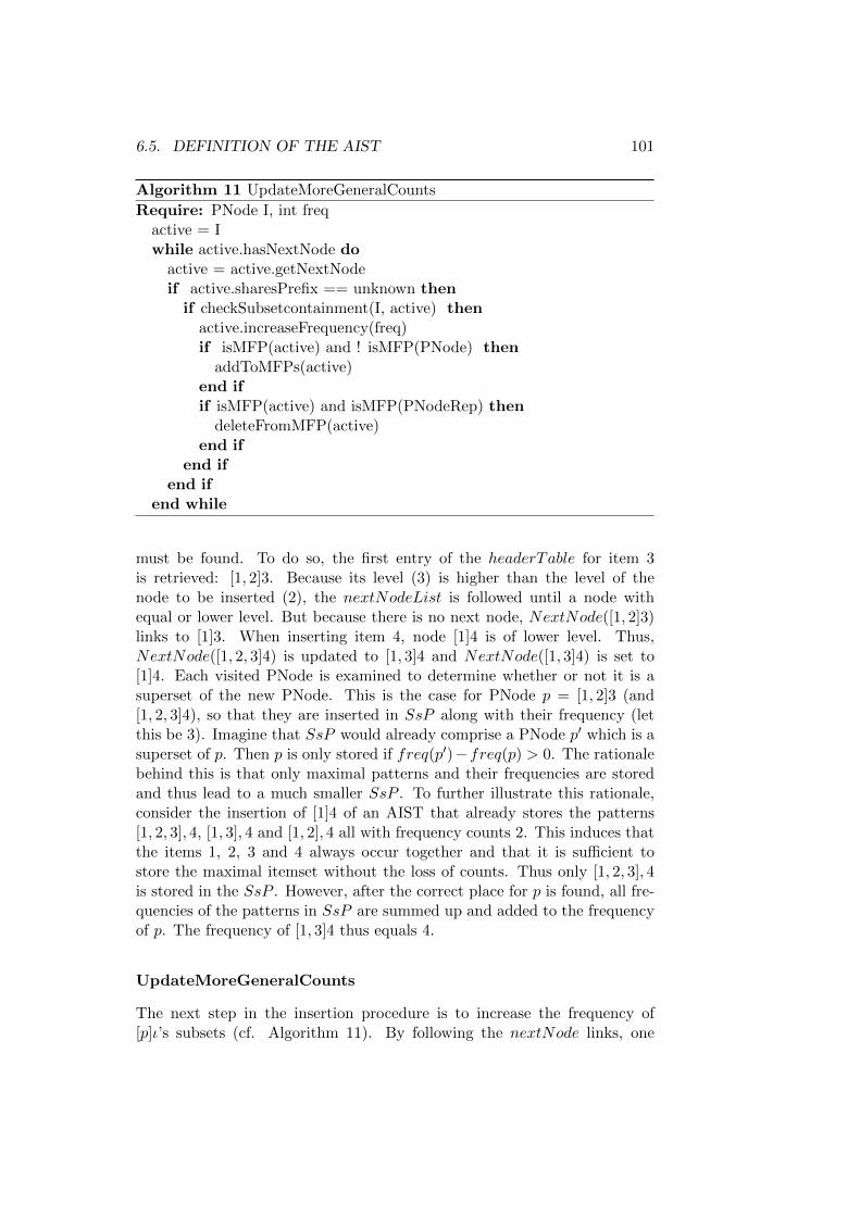
6.5. DEFINITION OF THE AIST 101
Algorithm 11 UpdateMoreGeneralCounts
Require: PNode I, int freqactive = Iwhile active.hasNextNode do
active = active.getNextNodeif active.sharesPrefix == unknown then
if checkSubsetcontainment(I, active) thenactive.increaseFrequency(freq)if isMFP(active) and ! isMFP(PNode) then
addToMFPs(active)end ifif isMFP(active) and isMFP(PNodeRep) then
deleteFromMFP(active)end if
end ifend if
end while
must be found. To do so, the first entry of the headerTable for item 3is retrieved: [1, 2]3. Because its level (3) is higher than the level of thenode to be inserted (2), the nextNodeList is followed until a node withequal or lower level. But because there is no next node, NextNode([1, 2]3)links to [1]3. When inserting item 4, node [1]4 is of lower level. Thus,NextNode([1, 2, 3]4) is updated to [1, 3]4 and NextNode([1, 3]4) is set to[1]4. Each visited PNode is examined to determine whether or not it is asuperset of the new PNode. This is the case for PNode p = [1, 2]3 (and[1, 2, 3]4), so that they are inserted in SsP along with their frequency (letthis be 3). Imagine that SsP would already comprise a PNode p′ which is asuperset of p. Then p is only stored if freq(p′)−freq(p) > 0. The rationalebehind this is that only maximal patterns and their frequencies are storedand thus lead to a much smaller SsP . To further illustrate this rationale,consider the insertion of [1]4 of an AIST that already stores the patterns[1, 2, 3], 4, [1, 3], 4 and [1, 2], 4 all with frequency counts 2. This induces thatthe items 1, 2, 3 and 4 always occur together and that it is sufficient tostore the maximal itemset without the loss of counts. Thus only [1, 2, 3], 4is stored in the SsP . However, after the correct place for p is found, all fre-quencies of the patterns in SsP are summed up and added to the frequencyof p. The frequency of [1, 3]4 thus equals 4.
UpdateMoreGeneralCounts
The next step in the insertion procedure is to increase the frequency of[p]ι’s subsets (cf. Algorithm 11). By following the nextNode links, one
102 CHAPTER 6. AUGEMENTED ITEMSET TREES
can decide whether or not another pattern in the AIST is a subset of [p]ι:[p′]ι ≺ [p]ι. To speed up the subset check, a flag called sharesPrefix isintroduced. The intuition behind this flag is that due to the canonical or-dering in the tree, subset-checks can be reduced to look-ups, if the parent ofa PNode [p′]ι was already visited during the insertion. It can take the values{unknown, true, false} and indicates whether the node [p′]ι was already vis-ited during the insertion process. The subfunction checkSubsetcontainmentreturns true, if [p′]ι’s sharesPrefix flag is true and false, respectively.Then, Node [p]ι is updated with this result. If [p′]ι was not yet visited(unknown is returned) a complete check for subset containment is per-formed, by subsequent parent comparisons.
Example: Reconsider the tree in Figure 6.2 where pattern p = {1, 3, 4}was inserted. Subsequent to its own frequency adaptation, each subpattern’sfrequency must be updated as well. Here, the sharesPrefix-flag of thePNode []1 on the path to [1, 3]4 has already been set to true. When updatingall subsets of pattern [1, 3]4, the first PNode considered is [1]4, because it isthe first PNode after p in p’s nextNodeList. The parent of [1]4 is PNode []1and thus sharesPrefix is set to true. This also implies that [1]4 is a subsetof [1, 2, 3]4, because its prefix [1] is a subset and the last item, 4 is equal.Therefore, its frequency is increased by p’s frequency. The second PNode inthe list is [2]4 with parent []2. Here the flag sharesPrefix is unknown anda full subset check must be performed. It will return false und thus [2]4’sfrequency is not increased. The last PNode to check is []4 with the root asfather where sharesPrefix is also set to true. It is therefore a subset of[1, 3]4, and again its frequency is increased.
6.5.2 Deleting MFPs
After a new pattern [p]ι was inserted in the AIST, all MFPs pr have to bechecked if they are still frequent and maximal. If there is a new patternp′r, which is more specific, pr is only deleted from the list of MFPs. How-ever, if the minsup constraint for pr is not fulfilled anymore, it also has to bedeleted from the MFPs list, and moreover, subsets of the pattern can still befrequent and are therefore examined concerning frequency and maximality.In general, a pattern of length l has l subsets of length (l − 1) that, in thiscase, must be checked one after another. Ideally, the enumeration of subsetsfollows a depth first search strategy so that if a frequent subset [p′]ι is found,all further subsets of [p′]ι can be pruned away from the search space. To en-sure both, completeness and non-redundancy during the generation process,the search is implemented in the following way: All subsets of [p]ι are cre-ated by deleting the IdxToDeleteth largest item of [p]ι. If subset [p′]ι is notfrequent, all subsets of [p′]ι are explored. Each created pattern is inserted

6.6. EXPERIMENTS 103
in the AIST with frequency zero falling back to Algorithm 8. Frequencyzero assures that no subsets are incorrectly incremented. In contrast, thecount of all supersets is added to the pattern. Subsequently, the resultingnode can be treated as any other node. However, this generation may alsoinclude candidates covering items which are not frequent anymore. Thismay lead to many unnecessary tests of subsets, because patterns containinginfrequent one-patterns cannot be frequent. Thus, excluding even few itemscan drastically reduce the search space. In order to find such items, eachentry in the header table is checked whether it is frequent or not. Then, theinitial candidate for each MFP is the MFP itself, where all infrequent itemsare excluded. This guarantees that all maximal frequent subsets are foundwithout considering useless subsets.
Example: To illustrate this strategy, imagine that a maximal pattern[1, 3]4 becomes infrequent, but two of its 2-subpatterns are frequent. Thesearch starts from pattern p = {1, 3, 4} (which is also the candidate, be-cause all one-items are frequent) and creates the first pattern to be tested:{1, 3} (the last item is removed). Because it is frequent, its subpatterns{1} and {3} are pruned away from the search space. The next pattern is{1, 4} which turns out to be infrequent. Therefore, the next pattern is cre-ated: {4}, which is again frequent. Pattern {1} is omitted here, because itwould have been enumerated after {1, 3}. Then, the last pattern’s ({3, 4})frequency is calculated, and this is again frequent. Because {3, 4} is nowalso maximal frequent, pattern {4} is deleted from the MFPs list. As nomore patterns are to be evaluated, search stops with a complete set of newMFPs.
6.6 Experiments
6.6.1 Data sets
The first data set is the diagnostic data introduced in Section 3.1.2. To de-rive different sized data sets, instances were randomly sampled of the wholedata set with 170,375 instances.Second, 18 data sets were generated by the IBM data set generator [2] whichis implemented in the (T)ARTool [66]. They cover a different number of pat-terns (P ∈ {50, 100, 1000}), average transaction lengths (AT ∈ {5, 10, 15})and average pattern length (AP ∈ {2, 4, 6}).1 For each P , six data sets(DS) with parameters (P,AT,AP ) were generated, assuring that AP is atmost half of AT : DS1 = (50, 5, 2), DS2 = (50, 10, 2), DS3 = (50, 10, 4), . . .,DS18 = (1000, 15, 6). Each data set holds 10,000 instances and consists of100 attributes, resulting in differently sparse data sets, with different trans-action and pattern lengths. These data sets were used to test the behavior
1The parameters were set following the suggestions in the original publication.

104 CHAPTER 6. AUGEMENTED ITEMSET TREES
Figure 6.3: Runtime depending on the number of instances of the diseasedata set with a minimum support of 0.1
of the algorithm for different pattern and transaction lengths for differenttypes of data sets. For scalability experiments, testing the performancefor different sizes of input instances, data sets with up to 2M transactions(P : 20, AT : 5, AP : 3) were generated, including either 10(I10) or 30(I30)attributes. Because they were each generated from scratch, they exhibit dif-ferent distributions of patterns. Note that in all these data sets, an instanceis composed of several patterns and also called a transaction.
6.6.2 Empirical evaluation
To evaluate the proposed method, the runtime and the size of the AISTdepending on the number of input instances, varying minimum support anddifferent data set characteristics are displayed. Moreover, a comparison tothree established methods for frequent itemset mining is drawn. Each ofthe following experiments was conducted on a 2.2 GHz machine with 1GBRAM. The AIST was implemented in Java.
A first evaluation compares the AIST to other pattern mining algorithms.The runtimes of AIST-based MFP mining, compared to the standard Apri-ori, FP-growth, LCM2 (a batch MFP miner) approach and a version ofCanTree are presented. A comparison against e.g., Moment, SWIM and
2Implementations from C. Borgelt and T. Uno, http://fimi.ua.ac.be/src/

6.6. EXPERIMENTS 105
Figure 6.4: Runtime for different data set sizes
DISC is not conducted, because these algorithms were created for a dif-ferent problem setting where instances may be observed more than once.Figure 6.3 presents the performance of miners for an increasing data setsize. As we are particularly interested in an online setting, the right handside of Figure 6.3 with more than 80,000 instances is most important. Notethat runtimes below 0.1s are not displayed in the figure, because of thelogarithmic scale. The runtimes show that, while A-priori is slower thanthe AIST approach, FP-growth and LCM (FP-growth is displayed exem-plarily) are more effective than the AIST. However, these three methodsonly calculate the MFP after all instances were observed. When applyingApriori, FP-growth and LCM to the incremental case, by repeatedly miningthe current set of MFPs, they are significantly slower than the proposedapproach, despite their very efficient mining and search strategies (LCMis slightly better than FP-Growth). In fact, every batch algorithm that isapplied repeatedly, will result in excessive runtimes: If the data set size is10l, the number of batch runs also grows exponentially with l, because ithas to be repeated 10l times. Next to that, the data set must be accessedfor each run, which can result in additional memory problems if the set be-comes large (l ≥ 6). Thus, a ‘repeated batch’ approach is not appropriatelarge data sets. As a last algorithm for the runtime comparison, CanTree[55] was exemplarily chosen from the group of algorithms that incrementallymine updated databases. It outperforms several other algorithms and hasa similar underlying data structure as the AIST. Thus, we interpreted the

106 CHAPTER 6. AUGEMENTED ITEMSET TREES
Minimum support 0.1 0.08 0.06 0.04 0.02
Runtime (s) ∼ 1 ∼ 1 2 7 >60
Table 6.1: Runtimes for different values of minimum support for 42,565instances of the disease data set
problem setting as an initially empty database where as many updates takeplace as instances are in the data set (data stream setting). Although itis better than the FP-growth approach, it is still not faster than the AISTimplementation. This is mainly due to the repeated creation of projecteddatabases on which it mines the frequent patterns. This is indeed very effi-cient when only few updates take place, but slows down the mining processfor many database updates.The second evaluation targets the runtime for different numbers of minimumsupport. Table 6.1 gives the runtime, beginning at a minimum support of0.1 (larger values always resulted in a runtime below one second). The run-time increases for smaller values for the minimum support, because moreMFPs are found, which must be updated. This can be very expensive whenlarge patterns become infrequent.A third experiment examines the behavior of the algorithm for different dataset types. Table 6.2 displays the runtime for the IBM data sets. The bestruntimes are achieved for small transaction sizes consisting of few patterns(column 1, 7 and 13). In contrast, for great transactions that additionallyconsist of many small frequent patterns, the search may be very expensive(column 4, 10 and 16): If patterns in the data are small but the currentcandidate c is large, a worst case search time of O(2|c|) may happen. How-ever, long transactions with few, but large patterns can be mined moreefficiently, because much less candidates are inspected. Additionally, thesenumbers show that denser data sets not necessarily lead to a longer run-time, but that the transaction and pattern lengths restrict the algorithmto either transactions of few large patterns or sparse data sets with smallinstances. Next, we address the algorithm’s scalability. Figure 6.4 showsthe runtime for several large data sets and different minimum support val-ues. The two data set I10 Minsup 0.1 and I10 Minsup 0.1 2G are bothdata sets with 10 attributes, where the minimum support is set to 0.1. Thedifference is that the curve I10 Minsup 0.1 is composed of different datasets, (for each data set size a new data set was created), while the secondcurve displays the subsequent runtimes of the 2 million instances (one dataset only). The first curve shows how the runtime varies between randomdata sets, while the second displays the runtime, when more and more in-stances of the same data set are taken into account. All data sets (exceptI10 Minsup 0.1 2G) show that larger data sets may not necessarily result inlonger runtimes. Again, this is due to the distribution of patterns in the data

6.6. EXPERIMENTS 107
P 50 100Density
AT 5 10 15 5 10 15AP 2 2 4 2 4 6 2 2 4 2 4 6
Runtime (s) 0 14 9 98 55 48 0 18 11 188 43 50
P 1000Density
AT 5 10 15AP 2 2 4 2 4 6
Runtime (s) 1 18 11 43 42 50
Table 6.2: Runtimes for the IBM data sets. Each block represents the dataset created using a fixed P. The first line gives the transaction size of thedata set, while the second line shows the pattern size (cf. Section 6.6.1). Themaximal and minimal values per P-block are indicated in bold. P: Numberof Patters, AT: transaction size, AP: pattern size
set. Large, but infrequent patterns as well as many MFPs may increase theruntime. Take curves I30 Minsup 0.5 and I10 Minsup 0.5 as an example:using more attributes does not necessarily induce a higher runtime (com-pare Number of Instances = 105 vs. Number of Instances = 2 ∗ 105).The distribution of frequent patterns and the average size is crucial for thesuccess of the algorithm. However, the runtime of one large data set forsuccessive operation steps (I10 Minsup 0.1 2G) shows the expected linearruntime for increasing data set sizes.The last two evaluations examine first, the size of the AIST and second,the corresponding memory requirement for different data sizes and densi-ties. Figure 6.5 gives the successive sizes of the AIST for the IBM data setsand shows the influence of the specific data set parameters AP , AT and P .Note that for a better visualization not every curve is displayed. Moreover,Figure 6.6 shows how the size of the AIST is influenced by different numbersof attributes in the data. Considering P (number of patterns), the size ofthe AIST grows with more patterns (cf. Figure 6.5). The lines of (5 50 2),(5 100 2) and (5 1000 2) clearly show this relation. This is of course trivial,the more patterns exists in the data, the more nodes must be present tocapture them. The opposite is the case for the average pattern size (AP ).The larger AP , the smaller the tree becomes: the search for larger patternsis quicker, because fewer candidate patterns have to be created and tested.The graphs (15 100 2), (15 100 4) and (15 100 6) show this relationship. TheAIST of (15 100 6) is the smallest. The influence of AT is illustrated by lines(5 100 2), (10 100 2) and (15 100 2). The greater the average transactionsize, the larger the AIST. The reason for this lies in the creation of data. Atransaction consists of frequent patterns, the larger the predefined size fora transaction, the more patterns are in it. Then, the AIST has to separate

108 CHAPTER 6. AUGEMENTED ITEMSET TREES
Figure 6.5: Number of nodes of the AIST for different data set parameters.The numbers in brackets correspond to (AT, P, AP) as described in Section6.6.1. The first point for each line indicates the value for 100 instances.
Figure 6.6: Number of nodes of the AIST for 2G data sets and differentvalues of minimum support

6.6. EXPERIMENTS 109
these patterns again, which means that small subsets of large transactionshave to be found. To do so, many nodes have to be created and evaluated.Now let us consider how the size of an AIST depends on the number ofattributes in the data set. Each data set in Figure 6.5 has 100 attributes,while the data sets of Figure 6.6 contain 30 and 10 attributes. The ranges ofthe AIST sizes vary between 104 − 105 for data sets with 100, 103 − 104 for30 and below 103 for 10 attributes, respectively. The explanation for thisis that despite only a subset of possible patterns is evaluated, the patternscreated for a data set vary stronger for many attributes, which increasesthe AIST. However, data sets with many attributes may nevertheless resultin a smaller tree, if the transaction size or pattern size is appropriate. Afurther question is, whether the size of the AIST will saturate after a certainnumber of instances and how fast it is growing. At first glance, for smallvalues of P the AIST is not growing extraordinarily for more than 7,000patterns (cf. Figure 6.5 (5 50 2)). It seems that all important patterns arealready incorporated into the tree and only few new patterns are added.Although this limit cannot be observed for the remaining curves, the slopefor each curve is decreasing steadily. This also suggests that even for moredifficult data sets the AIST will reach a steady level. If only few attributesare present in a data set, saturation is reached very quickly. Figure 6.6 givesan example for that, the final AIST for data set I10 is created after only afew hundred examples.Considering the initial increase of the curve, one exceptional large one showsgraph (15 50 2). It is the steepest ‘start’ for all presented data sets. In fact,(15 50 4) should be smaller than (15 100 4), because it has less patterns,but the same average transaction and pattern size. A possible explanationfor this is that the more patterns were created for a data set, the higher thechance that these patterns overlap (they share items). Then the overlappingparts seem to be frequent maximal patterns in the beginning, because theyoccur frequently. However, later they will turn out to be infrequent or notmaximal. Thus the slope of (15 100 4) and (15 1000 4) (not illustrated) issignificantly greater than for (15 50 4). The size of the their AISTs will ex-ceed the one of (15 50 4) after approximately 20*103 and 15*103 instances,respectively. In general, one can expect that the size of an AIST initiallygrows quicker for large transaction sizes and small pattern sizes.Concerning the size of the AIST dependent on the minimum support, Fig-ure 6.6 shows that the AIST increases for lower minimum supports (cf.I30 0.5 2G vs. I30 0.1 2G). Candidates are greater if the minimum supportis low, which again increases the search space. Then more candidates mustbe incorporated into the AIST. Although these findings give a hint for thesize and the growth rate for an AIST, its final size is of course also dependenton the actual patterns in the data set, the minimum support and the orderof the instances. A good example for this is given by (10 100 2) and (10 1004). Their size is nearly equal, instead of (10 100 2) being larger. The reason

110 CHAPTER 6. AUGEMENTED ITEMSET TREES
for this can be that most of the patterns of (10 100 2) are detected early orthat a better ordering of the instances may lead to a more compact AIST.The last experiment adresses the memory requirement of the AIST (not il-lustrated). We computed the RAM usage for the AIST-task while processingthe I30 0.5 2G data set. The time between RAM allocation increases dur-ing the process and the final RAM allocation is 50KB for the whole AIST.Altogether, these experiments lead to the conclusion that the AIST is anappropriate data structure for large frequent patterns and can be applied todifferent types of data sets. In particular for larger patterns, the savings canbe marked. Consider a standard bottom up search strategy that needs toexplore nearly the whole pattern space to find the MFPs. For data sets of100 attributes about 1.27*1030 frequent patterns must be evaluated. Com-paring this number to the sizes of the resulting AISTs, savings of severalorders of magnitude can be observed. However, the fewer attributes, the lesssavings are achieved, for 30 attributes 99.99% of the search can be omitted,while it is only 50% for a data set of 10 attributes. These numbers may befurther reduced, when the patterns are small (|p| < 1
2 ∗ |I|). Then a bottomup search strategy may be more appropriate.
6.7 Conclusion
We introduced a data structure that allows for instance-incremental miningfor maximal frequent patterns (MFPs). Our setting differs from related set-tings [18, 63, 20, 32] in that we assume that instances arrive one by one, arenot stored, and MFPs of the complete datastream are desired. Combiningan IST-like data structure with FP-tree elements in a data structure calledAIST (augmented itemset tree), we ensure that the MFPs are up to datefor each new instance at any point in time. Nodes (patterns) containing thesame item are connected and thus the number of necessary subset checks,while updating the frequencies of observed patterns, is decreased. To eval-uate the proposed algorithm, we examined the runtime and the size of theAIST depending on the number of input instances, minimum support values,data set characteristics and compared it to several alternative approaches.We conclude that this method can be applied to very large binary data setswhen maximal frequent itemsets can be expected to be large. In future work,we plan to adapt and use the AIST for batch-incremental mining. Second,we want to apply the AIST in an MFP-based clustering (which gave us themain motivation for developing the data structure for this setting in the firstplace), where MFPs are the representers of clusters. Here, the successiveand quick update of MFPs should be useful for efficiently extracting themain properties of clusters for very large binary data sets.

Chapter 7
Using Constraints on theAttribute Level for PRTAInduction (CSPRTA)
Like in other machine learning models, background knowledge should beincorporated into the learning process of PRTAs. This is especially use-ful in the domain of disease pattern analyses. There, physicians or othermedical experts often want to concentrate on their individual area of exper-tise. Moreover, they are only interested in a specific question, e.g. how acertain subgroup of patients behaves or develops. In the domain of PRTAinduction, a physician may want to examine how a specific group of pa-tients corresponds to a treatment compared to another group. Therefore,the induction process must be provided with a definition of the group(s) ofinterest. Then, the resulting paths (or states of the groups) can be evalu-ated by the physician and differences in the developement of patients aredisplayed. As such definitions in the medical domain often rely on patientcharacteristic descriptions that correspond to the level of attributes, theconstraints must also be defined and implemented at the attribute level. Inthis chapter, we first introduce constraints on the attribute level and thenpresent an implementation for the induction of automata by an attributeconstrained clustering (ACC). Last, we show how the constraints alter theresulting states of the automaton. Related work and further details aboutthe scalability, extensibility and generality will be given in the next section,while this chaper focuses mainly on the applicability for the detection ofautomata.
7.1 Main Idea of Attribute Level Constraints
As described above, in the medical domain there is a strong need to describegroups of patients, which is of course done by their characteristics. Further-
111

112 CHAPTER 7. ACC IN PRTA INDUCTION
more, such a description should be used to guide the expected results of adata evaluation step. Therefore, we propose to use a new type of constraint:attribute level constraints (cf. Section 8) that specify how instances having acertain characteristic should be treated in the PRTA induction process. Fre-quently, groups of patients having the same characteristics should be found,which induces that all patients with the specific characteristics should beput in the same cluster. Then, a physician can inspect the distribution ofthe remaining attributes in the resulting cluster. Thus, the first proposedconstraint is the must-link (ml) constraint that ‘collects’ all patients thatshare a specific set of properties and forms a cluster with them. However,there is one problem: How to deal with patients that do not have the spec-ified characteristics but are similar to this set of patients. In the case thatonly the patients that show the specific characteristics are to be combined,then this condition should also be expressed by a constraint. Therefore,the second proposed constraint is the must-link-exclusive (mlx) constraintthat ensures that only patients that satisfy the given condition are groupedtogether. This is of course a very strict condition, but is necessary in thecase when only the described group of patients is of interest. A formal de-scription of these two constraints is given in Section 8.2.2 and 8.2.3, so thatonly an informal description of the problem setting is given here.
7.1.1 Problem Setting
Let D = {(x11, . . . , x
1m), . . . , (xn1 , . . . , x
nm)} be a data set of binary instances
(xij ∈ {0, 1}), m being the number of attributes and n the number of in-stances. Additionally, a set of attribute-level constraints Φ is provided. Aconstraint ϕ ∈ Φ is in general any formula in propositional logic rangingover the propositional variables x1 to xm. In the remainder of the chapter,the values 1 and 0 are interpreted as Boolean truth values, true and false.Although the propositional formulae could take any form in general (alsonormal forms, for instance), we restrict ourselves to conjunctions in the fol-lowing. In a formula, an unnegated literal xi means that the value of thatvariable has to be 1 in an instance, whereas a negated literal ¬xi meansthat the variable has to take the value 0. For each attribute-level constraintϕ ∈ Φ and instance xi, expression ϕ(xi) returns whether instance xi fulfillsconstraint ϕ, i.e. the instance is a model [37] for the constraint
ϕ(xi) = 1 ⇔ xi |= ϕ . (7.1)
If this is the case, we say that instance xi is in the scope of constraintϕ. Function z(Φ, C) returns whether a clustering C satisfies the specifiedconstraint set Φ. The conditions in which the constraints are satisfied aregiven in the following sections for each specific constraint type. Moreover,a clustering can be scored with an objective function f : C → R accordingto its quality. The overall goal is to induce an automaton that includes k

7.2. IMPLEMENTATION 113
states (that correspond to clusters) for the data set D such that the k statessatisfy the provided attribute-level constraints, z(Φ, C) = true, and that fis maximized.
7.2 Implementation
This section shows how the two proposed constraints ml and mlx can beimplemented in the PRTA induction. As there are already several methodsproposed to derive a PRTA from data, this section focuses on the onlineinduction method with a previous PTA construction (cf. Chapter 5).
7.2.1 Implementation of must-link
This section shows how the ml constraints can be used in the induction ofPRTAs. Therefore, the algorithm SPRTA is adapted to incorporate con-straints (CSPRTA), which is introduced in the following (cf. Algorithm 12).To incorporate constraints on the attribute level in the SPRTA algorithm,
Algorithm 12 CSPRTAml (Histories H, double θ)
1: PTA pta = createPTA(H)2: clustering = initConstrAssignment(Φml)3: for all xi ∈ pta do4: if ∃ϕj ∈ Φml | xi � ϕj then5: assignInstanceToCluster(cj , clustering[ϕj .belongsToCluster()])6: else7: k = fNC(xi, C)8: if k 6= −1 then9: C[k].addInstance(xi, θ)
10: else11: k = C.addNewCluster();12: C[k].addInstance(xi, θ)13: end if14: end if15: end for16: validateAssignments(pta, C)17: for all Cj ∈ C do18: mergeAllInstancesOfCluster( Cj)19: end for
two adaptations have to be made. First, after the PTA creation, there isone cluster created to which exactly one constraint belongs: the constraint isassigned to that cluster. The reason for this is that the mlx constraint doesnot allow incorporate instances that do not entail it. To avoid a merge of twostates (where one of them does not entail the constraint) and a subsequent

114 CHAPTER 7. ACC IN PRTA INDUCTION
reallocation of the corresponding instances, the constraints are assigned toclusters right at the beginning of the induction process. As the implemen-tation for the ml constraint should the same, this is also implemented inthe same way for these constraints. This also ensures that all instances thatentail the ml constraint are put in one cluster, but still allows that otherinstances are grouped with them. Additionally, each cluster is only assignedone constraint. The reason for this is that we assume that the user ex-pects one cluster for each given constraint. Therefore, if a cluster had morethan one constraint, then the final number of constrained clusters would betoo small. The second adaptation takes place in the online clustering step.Then, each instance is evaluated as to whether it entails one of the givenconstraints. If this is the case, the instance is immediately placed in thecluster to which the constraint belongs. If an instance entails more thanone constraint, it is placed in the first constrained cluster that is found. Allinstances that are not in the scope of a constraint are placed in the nearestcluster. However, in the last step, the validation of the assignments, onlyinstances that do not entail a constraint are considered for reassignement.This ensures that each instance is placed to its corresponding constraint.
Algorithm 13 CSIPRTAmlx (Histories H, double θ)
1: PTA pta = createPTA(H)2: clustering = initConstrAssignment(Φml)3: for all xi ∈ pta do4: if ∃ϕj ∈ Φmlx | xi � ϕj then5: assignInstanceToCluster(cj , clustering[ϕj .belongsToCluster()])6: else7: k = fNC(xi, C)8: if k 6= −1 then9: while violatesConstraint(xi, clustering.getΦmlx()) do
10: clustering = fNC(xi, clustering, p++)11: end while12: C[k].addInstance(xi, θ)13: else14: k = C.addNewCluster();15: C[k].addInstance(xi, θ)16: end if17: end if18: end for19: validateAssignments(pta, C)20: for all Cj ∈ C do21: mergeAllInstancesOfCluster( Cj)22: end for

7.3. EXPERIMENTS 115
7.2.2 Implementation of must-link-exclusive
As another interesting constraint, the mlx should be incorporated into theCSIPRTA algorithm. The difference between the mlx and the ml constraintis that only instances that are in the scope of the mlx constraint may be,and must be, placed in the cluster. On the other hand, a cluster with anml constraint can also have instances outside of its scope assigned to it.Such a constraint creates clusters of instances that share a specific amountof characteristics, which may be interesting to the user. Algorithm 13 showshow such constraints can be used in the induction of PRTAs. In addition tothe adaptations of the ml constraint, there is another evaluation to satisfyall mlx constraints. This is shown in lines 9 to 10. If an instance shouldbe placed in a mlx-constrained cluster, this instance must not violate theconstraint, i.e. it must be in the scope of the constraint. If this is notthe case, the instance must also not be placed in the corresponding cluster.Then, the nearest cluster in line is retrieved and again checked whether theinstance violates the constraint. This is repeated until a cluster is foundin which the instance may be placed. If there is no such a cluster, a newcluster is created and the instance is placed into this one. The remainingpart of the algorithm corresponds to the SIPRTA algorithm.
7.3 Experiments
This section focuses on the results of the experiments when using such at-tribute level constraints for the induction of automata. Moreover, ways todefine manageable constraints will be discussed. However, there is one algo-rithmic adaptation to show the power of constraints. Here, we do not makeuse of the validateAssignments which is mainly used to correct instancesthat we misplaced in ’wrong’ clusters in the beginning of the clustering step,where the cluster-size condition (cf. Section 5.1.3) was not yet as strict asin the end. In contrast, when constraints are included, the user restricts theplacement of instances a priori such that a misplacement cannot take place.
7.3.1 Synthetic Constraints
The first experiment addresses the behavior of the synthetic automaton thatincludes constraints. To show the applicability of the attribute constraints,we first created an automaton without constraints. This automaton is illus-trated in Figure 7.1a. It shows that although the algorithm is capable ofidentifying the correct maximum frequent patterns per state, there are manywrong transitions and some states are blurred due to the inclusion of eventsthat should in fact be place in other states. One example for this problemis state 3 which combines some states from state 1. This is ascribed to theinitial phase of the clustering, where event [3, 5, 8, 10] shares two items with

116 CHAPTER 7. ACC IN PRTA INDUCTION
(a) Result for the unconstrained SPRTAalgorithm without the validate assignmentprocedure. The representer (MFP) foreach state is shown in brackets.
(b) Result of the CSPRTA algorithm forthe synthetic data set and constraint mle1.
(c) Result of the CSPRTA algorithm forthe synthetic data set and constraints mle1and mle2.
(d) Result of the CSPRTA algorithm forthe synthetic data set and constraints mle1,mle2, mle3 and mle4.
Figure 7.1: Resulting automata by a stepwise inclusion of the constraints
events [3,5] that are placed in a small cluster. Then [3, 5, 8, 10] may thereforebe assigned to the same cluster. The same is true for state 7. Neverthe-less, attribute constraints can be used to address this problem. Therefore,we first introduce a constraint that collects all events [3, 5, 8, 10] into onestate: mle1 = (3 ∧ 5 ∧ 8 ∧ 10) and thus separates states 3 and 1. Figure7.1b shows that the inclusion of this single constraint erases four erroneoustransitions and also makes the distinction of profiles better. But still, thereis one problem with state 6 – one transition to state 5 is missing (as wellas the transition to state 7). Moreover, the distinction between state 9 andstate 10 is difficult when considering the profiles, which is due to the factthat there are some events clustered to state 9 that should have been withstate 5. To fix these two problems we introduce three more constraints:
• mle2 = (1 ∧ 3 ∧ 9 ∧ 10)
• mle3 = (2 ∧ 5 ∧ 6 ∧ 7 ∧ 8 ∧ 9)
7.3. EXPERIMENTS 117
• mle4 = (2 ∧ 5 ∧ 6 ∧ 7).
They are included in the CSPRTA algorithm in two steps. Figure 7.1c showsthat this was quite a good choice, because the missing transitions from state6 appear again as well as their correct direction. However, using the mlxconstraint also comes with a drawback here: an additional state appearedthat comprises events 〈1, 2,∗ 〉 and 〈1,∗ , 9, 10〉 which are deviations of states10 and 6. [1,9,10] cannot be included in state 6 because of the mlx constraintand probably by accident [1,2] is also included in this state. However, thefrequency counts of this node as well as the transition probabilities wouldsuggest to the user that this node is an exception. Now mlx3 and mlx4
should be included in the model, because state 9 holds some events of state10. Note that the single inclusion of mlx4 would not result in a correctmodel, because then, states 9 and 5 would be combined into a single one asthe profile of state 9 is a subset of state 5. Therefore, a constraint that alsocombines the events of state 5 is needed. Figure 7.1d shows the result ofthis operation. The structure of the automaton is nearly correct, but stillthere are three remaining transitions that are wrong. One experiment to testwhether it is possible to leave out, e.g. mlx2 showed that this is not possiblebecause then states 8 and 6 would be placed in one cluster. Summarizingthese experiments, one can see that constraints may improve the final model.Interestingly, they mainly do not influence the resulting profiles or states’representers but rather the transitions, by avoiding erroneous assignmentsof events during the beginning phase of the SPRTA clustering step. Second,literals that can express that an attribute is not present should be used toconstrain ’small’ states. This would be very helpful to identify states havingonly one or two attributes in their profile, like e.g., state 4. If constraintswould be used that only include few positive literals (’small’ constraints)then too many events would be clustered together and the final result wouldbe misleading. Therefore, the creation of constraints must be done verycarefully. Then, for such small automata it is not useful to incorporate mustlink constraints, although they are capable of summarizing all necessaryinstances: In an early timepoint of the clustering process, there may beother nodes that should not be put in that cluster, but are, because theyare still just similar enough. Finally, there are still some transitions thatare not yet correct. This shows that constraints may guide the inductionprocess, but are not capable to guarantee correct results.
7.3.2 Yeast Constraints
This section shows how the yeast automaton can be constrained. First,Figure 7.2 shows the resulting automaton, when SPRTA is run without thevalidateAssignments procedure. Although the cyclic structure is of coursevisible, first note that two states are highly similar (state 3 and state 5).Secondly, there is an additional transition from state 5 to state 3 (dashed
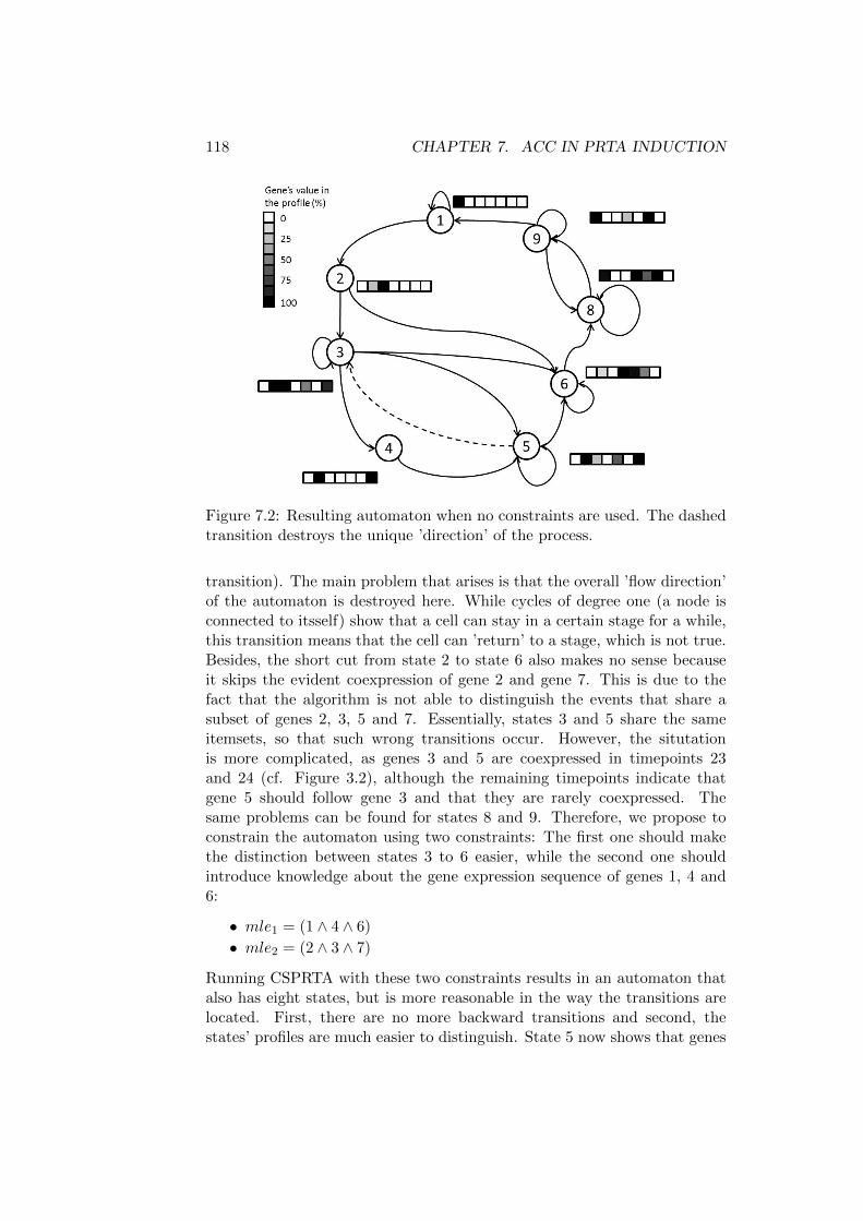
118 CHAPTER 7. ACC IN PRTA INDUCTION
Figure 7.2: Resulting automaton when no constraints are used. The dashedtransition destroys the unique ’direction’ of the process.
transition). The main problem that arises is that the overall ’flow direction’of the automaton is destroyed here. While cycles of degree one (a node isconnected to itsself) show that a cell can stay in a certain stage for a while,this transition means that the cell can ’return’ to a stage, which is not true.Besides, the short cut from state 2 to state 6 also makes no sense becauseit skips the evident coexpression of gene 2 and gene 7. This is due to thefact that the algorithm is not able to distinguish the events that share asubset of genes 2, 3, 5 and 7. Essentially, states 3 and 5 share the sameitemsets, so that such wrong transitions occur. However, the situtationis more complicated, as genes 3 and 5 are coexpressed in timepoints 23and 24 (cf. Figure 3.2), although the remaining timepoints indicate thatgene 5 should follow gene 3 and that they are rarely coexpressed. Thesame problems can be found for states 8 and 9. Therefore, we propose toconstrain the automaton using two constraints: The first one should makethe distinction between states 3 to 6 easier, while the second one shouldintroduce knowledge about the gene expression sequence of genes 1, 4 and6:
• mle1 = (1 ∧ 4 ∧ 6)
• mle2 = (2 ∧ 3 ∧ 7)
Running CSPRTA with these two constraints results in an automaton thatalso has eight states, but is more reasonable in the way the transitions arelocated. First, there are no more backward transitions and second, thestates’ profiles are much easier to distinguish. State 5 now shows that genes

7.3. EXPERIMENTS 119
genes1 2 3 4 5 6 7
Mfp 1 •Mfp 2 •Mfp 3u • • • •Mfp 3c • • •Mfp 4 • •Mfp 5 • • •Mfp 6 • • •Mfp 7 • • • •Mfp 8 • •
Table 7.1: Maximal frequent patterns for the yeast data set; with and with-out constraints. Note that Mfp4 was identified for the constrained automa-ton (c), while Mfp3 was induced in the unconstrained (u) one.
Figure 7.3: Result of the constrained yeast automaton

120 CHAPTER 7. ACC IN PRTA INDUCTION
Element Name Interpretation
WBC ratio of white blood cellsHGB HaemoglobineHCT ratio of solid blood
componentsRBC ratio of red blood cellsPLT ratio of blood platesCRP C-reactive protein inflammation indicator, risk
factor for heart attacks (HA)LDH Lactat-Dehydrogenase organ destruction indicatorCRE Creatinine bladder problems indicatorGOT Aspartat-Aminotransferase liver problems, acute oxygen
undersupply, heart attackGPT Alanin-Aminotransferase liver problemsUN blood urea nitrogen protein degradation, (HA) ind.
Table 7.2: Elements of the blood count and their interpretation
2,5 and 7 often occur together after genes 2,3 and 7 occured together. State4 indicates that gene 3 is not necessarily replaced immediately by gene 5but that there may also be a timespan, where neither gene 3 nor gene 5is active. Then, states 7 and 8 also show that genes 1,4 and 6 frequentlyoccur together before gene 6 is switched off. Table 7.1 displays the maximalfrequent patterns of both automata. It is very interesting that the SPRTAapproach and the CSPRTA approach identify nearly the same representersper cluster, but still CSPRTA manages to identify the transitions better.
7.3.3 Hepatitis Constraints
The Hepatitis data set is a rather hard one for the given algorithm of au-tomata induction. This is due to the fact that it is dense, i.e. each instanceconsists of many attributes. When running the induction algorithm withoutconstraints, one also sees that there are many clusters having several max-imum frequent patterns as representers. Therefore, the constraints shouldfocus on the combination of interesting similar patterns to first reduce thenumber of resulting clusters and to focus on a special kind of patients. Theattributes that are used in this data set are again summarized in Table 7.2.One interesting question for a physician would be to compare patients with abad blood count to ones having a normal blood count. The frequency distri-bution of the values shows that there are quite a few patients that have a nor-mal blood count (normal values of WBC, HGB, HCT, RBC and PLT), butthere are also patients that have values that are too low, e.g. HGB. In con-trast, excessively high values values are rare, cf. for example HGB and HCT,there are only 2 cases where they are too high. Therefore, we define a state

7.3. EXPERIMENTS 121
Figure 7.4: Comparison of patients having a normal (group 1) and a badblood count (group 2). Red bars indicate the frequency of the blood countelements for group 2, while the green bars show the distribution for group1.
’bad blood count’ (BBC) that summarizes patients with low values for HGB,HCT and RBC (PLT and WBC were left out because of their low frequency)and a state ’normal blood count’ (NBC): mle1 = (HGBL∧HCTL∧RBCL),mle2 = (HGBN ∧HCTN ∧RBCN ∧WBCN ). Figure 7.4 shows the result ofthis comparison analysis, i.e. the profiles of the resulting constrained statesare shown. Both states contain many events (NBC: 544, BBC: 709) and arehighly connected to other states (34 and 35 outgoing and 33 / 38 incomingtransitions). However, patients with BBC also show abnormal blood countvalues for the remaining elements. Notably, they are the only ones were high(low) values for CRP (UN) can be observed. Moreover, BBC-patients alsosuffer from a high GOT-value more frequently than NBC-patients, whichshows an acute oxygen undersupply, which may, e.g. cause a heart attack.This leads to another interesting question: how do patients look that havea high risk of a heart attack (the GOT and UN values are high). Therefore,we designed another constraint that captures patients with these properties:mle3 = (GOTH ∧ UNH). The resulting state combines 136 events and has33 (34) out (incoming) transitions. These patients also show a high valueof LDH that also indicates some kind of organ damage. Interestingly, theCRP-value is probably low, which shows that there are no current inflam-mations.Although these analyses give a good overview of the comorbidities of thepatients, another interesting analysis would be to observe their progression.However, this data set remains unsuited for this problem, because the re-sulting states are all highly connected among each other so that no obviouspaths can be seen. Nevertheless, this data set gives a very good impressionof how medically interesting constraints can be formed and inspected byusing the CSPRTA methodology.

122 CHAPTER 7. ACC IN PRTA INDUCTION
Figure 7.5: Profile of patients having a high risk of heart attack (UN andCRP are high and colored in red)
7.4 Conclusion
In this chapter we showed how the two attribute level constraints must-linkand must-link-exclusive can be incorporated and used in the SPRTA envi-ronment. Therefore, we adopted the implementation details presented inChapter 8 to fit the SPRTA algorithm. Most importantly, we showed inthe experimental part, how to design constraints, their benefits and short-comings on three different types of data. Using very specific constraints,i.e. constraints that consist of many literals, seems to lead to understand-able results. Including only a small number of literals instead, may blurthe resulting automaton. Besides, using must-link-exclusive constraints iseasier than the must-link constraints, as the user can directly form expectedstates. Moreover, attribute constraints seem not to work for the correctionof the states’ profiles, but work well for the correction of transitional er-rors. Altogether, including attribute level constraints may be well suited forthe evaluation of specific groups of events, but still the constraints must becarefully designed.

Chapter 8
Attribute ConstrainedClustering
Clustering is a frequently used method to analyze and segment data setsand for many applications, users wish to include their knowledge about theexpected result. Including such background knowledge in the form of con-straints may improve the clustering result or even drastically reduce theruntime. This is why researchers addressed the problem of defining andevaluating different types of constraints [100] in various cluster algorithmsin the past decade. The first idea of such constraints was to restrict theinstances that must (must-link) or may not (cannot-link) be grouped into acluster. This type of constraint is called instance-level constraint. However,background knowledge is not only present on the instance level. There alsois domain knowledge that can be expressed without even knowing specificinstances of a given data set. Therefore, we introduce a new type of con-straints: constraints on the attribute level, i.e. the properties of the instancesin a cluster are described instead of the relationships between the instancesthemselves. We call this type of constrained clustering attribute-constrainedclustering (ACC) [77].1 This type of constraint has one additional bene-fit compared to the known instance-level constraints: the representation ofbackground knowledge is much more compact when given on the attributelevel and thus addresses one important factor of constrained mining [24].Although the approach is not restricted to it, we focus on constraints thatspecify how instances with given attribute characteristics must be combined.In summary, the contributions of this chapter are as follows:
• First, we introduce must-Link and must-Link-Excl constraints on theattribute level in Section 8.2.
• Second, the direct incorporation into a popular clustering algorithm(k-Medoids) is presented (cf. Sections 8.2.2 and 8.2.3).
1This is an extension of previous work [11].
123

124 CHAPTER 8. ATTRIBUTE CONSTRAINED CLUSTERING
• Moreover, constraints on the attribute level are shown to be morecompact (Section 8.3.3) than on the instance level and experimentallydemonstrated to be useful when the background knowledge can beexpressed by instance characteristics (Section 8.3).
• Last, the relation to the well known instance-level constraints is es-tablished for each type of attribute-level constraint (cf. Sections 8.2.2and 8.2.3).
8.1 Related Work
The first clustering constraints in the literature were so-called must-link andcannot-Link constraints, which were incorporated into several algorithms,e.g. k-Means [100] and divisive clustering [50]. One main goal was to spec-ify the types of constraints and to show how heuristics can be used to finda near-optimal clustering solution that satisfies all constraints. This was in-vestigated, e.g. in the context of the k-Means algorithm [24, 25]. Especiallythe use of must-Link and cannot-Link constraints as well as cluster distanceconstraints were evaluated as to whether there exists a partition that satis-fies the given constraints and if it is actually possible to find it. Moreover,the scalability of must-Link and cannot-Link constraints and the modifica-tion of clustering approaches using the nearest-representative property werestudied [89]. Although it is acknowledged that attribute-level constraintsare important [101], they have not yet been explored extensively. One ap-proach applied one type of attribute-level constraint to co-clustering [71, 70].The proposed algorithm uses local bi-sets that are clustered to a final so-lution. In the clustering procedure, a k-Means-like process evaluates localanti-patterns for their correctness. The proposed constraint is not definedin general, but for specific attributes only, and may only be extended topairs of attributes. In particular, the constraint can only be applied if thecorresponding attribute is ordered, like a time stamp for the instance. More-over, the attribute must be numeric and thus, the constraint may be definedon an interval or non-interval scale. A similar constraint setting is usedto also define range-constraints on attributes in a cluster [23]. Again, theconstraint is applied on a single numeric attribute and the constraints arenot associated, i.e. they are independent of each other. To sum up, workin this area so far introduces constraints on the attribute level, but onlylinks pairs of attributes at most, and not sets in general. Additionally, theconstraints were incorporated into co-clustering, while this chapter aims forregular clustering, as we cannot guarantee to find optimal co-clusters. An-other type of constraints are cluster-level constraints [64]. The basic idea isto select clusters for a clustering out of a set of predefined possible clusters.The constraint then can define, e.g., which clusters must be incorporated inthe clustering or how large, complete or disjoint clusters may become. A

8.2. CONSTRAINTS ON THE ATTRIBUTE LEVEL 125
last approach to drive the clustering process is to define that patterns ingeneral (e.g., frequent itemsets) should be found in the final clusters [85].Although this approach also describes characteristics of clusters, no dataset specific knowledge can be provided to the mining algorithm. In sum-mary, attribute-level constraints are restricted in their expressiveness so far.In this chapter, we extend attribute-level constraints to a general form suchthat each attribute may be involved in a constraint. Additionally, we specifyproblem settings that benefit from such constraints.
8.2 Constraints on the Attribute Level
This section first introduces the necessary notation. Then, the proposedconstraints are formally defined including a running example. Subsequently,variations of the k-Medoids algorithm that incorporate the attribute-levelconstraints directly are presented.
8.2.1 Problem Description
Let D = {(x11, . . . , x
1m), . . . , (xn1 , . . . , x
nm)} be a data set of binary instances
(xij ∈ {0, 1}), m being the number of attributes and n the number of in-stances. Additionally, a set of attribute-level constraints Φ is provided. Aconstraint ϕ ∈ Φ is in general any formula in propositional logic rangingover the propositional variables x1 to xm. In the remainder of the chapter,the values 1 and 0 are interpreted as Boolean truth values, true and false.Although the propositional formulae could take any form in general (alsonormal forms, for instance), we restrict ourselves to conjunctions in the fol-lowing. In a formula, an unnegated literal xi means that the value of thatvariable has to be 1 in an instance, whereas a negated literal ¬xi meansthat the variable has to take the value 0. For each attribute-level constraintϕ ∈ Φ and instance xi, expression ϕ(xi) returns whether instance xi fulfillsconstraint ϕ, i.e. the instance is a model [37] for the constraint
ϕ(xi) = 1 ⇔ xi |= ϕ . (8.1)
If this is the case, we say that instance xi is in the scope of constraint ϕ.The task is, to group the instances xi ∈ D into a clustering that satisfiesthe given attribute-level constraints. A clustering C consists of k clustersC = {C1, . . . , Ck}, where each cluster is a set of instances Ci ⊆ D. Func-tion z(Φ, C) returns whether a clustering C satisfies the specified constraintset Φ. The conditions in which the constraints are satisfied, are given inthe following sections for each specific constraint type. Moreover, a clus-tering can be scored with an objective function f : C → R according to itsquality. The precise definition of this function depends on the applicationdomain. As an example one could consider the intra or inter cluster distance

126 CHAPTER 8. ATTRIBUTE CONSTRAINED CLUSTERING
or the silhouette coefficient [48]. Although constraints can be used in anyclustering scheme, this chapter presents how they can be included in thek-Medoids [48] algorithm. K-Medoids was chosen because it is a standard
Algorithm 14 k-Medoids (Dataset D, int k)
1: medoidsChange = true2: clustering = initializeClusterMedoid(k,D)3: while medoidsChange do4: for each Ii ∈ D do5: clustering = assignToNearestCluster(Ii, clustering)6: end for7: medoidsChange = calculateNewMedoids(clustering)8: end while
clustering algorithm that is fast, easy to modify and because it was fre-quently considered in the field of constrained mining. Algorithm 14 showsthe corresponding pseudocode. Summarizing, the overall goal is to find kclusters for the data set D such that they satisfy the provided attribute-levelconstraints, z(Φ, C) = true, and that f is maximized.
8.2.2 Must-Link
The first constraint, must-Link (ml), describes which instances must beclustered together due to their attribute characteristics. It is defined via thelogical formula given in Equation (8.2).
ϕ = ml(x1 ∧ . . . ∧ xm) (8.2)
A clustering C satisfies a set of must-Link constraints Φml, if and only if allinstances that are in the scope of a specific constraint ϕi ∈ Φml are groupedinto one cluster:
z(Φml, C) = true⇔∀ϕi ∈ Φml ∃Cl ∈ C ∀xk ∈ D : xk |= ϕi → xk ∈ Cl (8.3)
The must-Link constraint specifies that instances that are in the scope of aconstraint ϕi must be grouped in the same cluster Cl. Additionally, instancesthat are not in the scope of the constraint but are nearest to it, may also begrouped in that cluster. So, each cluster Cl contains the instances satisfyingthe constraint and additionally the closest instances:
Cl = {xk | xk |= ϕi} ∪ {xj | minC∈C
d(xj , C) = Cl}
Then, the must-Link ϕi is related to that cluster Cl. This relation is the keypoint to include attribute-level constraints in the clustering process. Each

8.2. CONSTRAINTS ON THE ATTRIBUTE LEVEL 127
instance can be checked whether it is in the scope of the ml constraint re-lated to the clustering. An instance is in the scope of a must-Link constraint,if it is a model for the constraint (cf. Formula 8.1), i.e. it has the necessaryattribute setting.Note that this type of constraint can also be related to the domain ofinstance-level constraints. More precisely, every attribute-level constraint ϕiinduces, for pairs of instances xk and xj within the scope of the constraint,a set of instance-level must-link constraints {mustLink(xk, xj) | xk |= ϕi ∧xj |= ϕi}. However, the ml constraint is not transformed into an instancelevel constraint but directly incorporated into the clustering process. Algo-rithm 15 shows the two main modifications necessary for the incorporationof must-Link constraints in the k-Medoids algorithm. The first adaptationensures that no initial medoid is in the scope of more than one must-Linkconstraint (line 2), which guarantees that each constraint is only related toone cluster. The second modification takes place in the clustering step. Ifan instances is in the scope of exactly one ml constraint ϕj (line 6), which isalready assigned to a cluster, then the instance will immediately be placedin the corresponding cluster. If several constraints apply, the one with thenearest corresponding medoid is chosen for assignment. If the instances are
Algorithm 15 ml-k-Medoids (data set D, int k, ml constraints Φml)
1: medoidsChange = true2: (clustering, assignedConstraints) =
initializeClusterMedoid(k,D,Φml)3: while medoidsChange do4: for all xi ∈ D do5: for all ϕj ∈ assignedConstraints do6: if xi � ϕj then7: assignToConstrainedCluster(xi, clustering, ϕj)8: belongstoCluster(xi) = true9: end if
10: end for11: if ! belongsToCluster(xi) then12: clustering = assignToNearestCluster(xi, clustering)13: for all ϕk ∈ unAssignedConstraints do14: if xi � ϕk then15: assignConstraintToCluster(ϕk, clustering)16: end if17: end for18: end if19: end for20: medoidsChange = calculateNewMedoids(clustering)21: end while

128 CHAPTER 8. ATTRIBUTE CONSTRAINED CLUSTERING
not in the scope of a related constraint (line 12), the usual assignment isconducted. Last, each constraint that is not yet assigned to a cluster isinspected whether the instance is in its scope. If this is the case, the con-straint is related to that cluster. In the following iterations, all instancesthat are in the scope of this constraint are then grouped into that cluster.Consider the following example: Let the database D comprise the followinginstances: D = {x1, . . . , x5}, where x1 = (1, 1, 0, 1, 0), x2 = (1, 1, 0, 0, 0),x3 = (0, 1, 0, 0, 0), x4 = (0, 0, 1, 0, 1) and x5 = (0, 0, 0, 0, 1). These instancesare to be grouped into two clusters (k = 2) and one must-Link constraint isprovided: ϕ1 = ml(x1 ∧ x2). Let instances x1 and x4 be the initial medoidsof the clustering. As instance x1 is already in the scope of the must-Linkconstraint, it is related to cluster 1. Due to the constraint, instance x2 isalso grouped into cluster 1. The remaining instances are assigned withoutconsidering the constraint. Instance x3 belongs to cluster 1, instance x5 tocluster 2. The resulting clustering C is thus C = {{x1, x2, x3}, {x4, x5}}.This constraint can be used to group instances that share one or severalproperties, no matter how the remaining attributes look like.
8.2.3 Must-Link-Excl
The second constraint, must-Link-Excl (mlx), is a modification of the must-Link constraint in a way that it not only defines which instances must begrouped together but moreover, which instances must not belong to thisgroup. Equation 8.4 shows when a clustering C satisfies such a constraintset Φmlx. This is the case, if only instances that are in the scope of amlx-constraint ϕi ∈ Φmlx are combined into a cluster.
z(Φmlx, C) = true⇔∀ϕi ∈ Φmlx ∃Cl ∈ C : ∀xk ∈ Cl : xk |= ϕi ∧@Cj ∈ C : Cj 6= Cl : ∃xm ∈ Cj : xm |= ϕi
(8.4)
Again, this constraint can also be expressed by a set of instance-level con-straints, more precisely, a set of must-Link and cannot-Link constraints:
{mustLink(xk, xj) | xk � ϕi ∧ xj � ϕi} ∪{cannotLink(xk, xj) | xk � ϕi ∧ xj 2 ϕi}
The first part is again a must-Link constraint which specifies that instanceswhich possess the given characteristics must be grouped together. However,for all instances that are not in the scope of the constraint, a cannot-Linkconstraint is induced. In this case the instance cannot be grouped to thecluster, it violates the constraint. Note, that although each attribute-levelconstraint can be transformed into an instance-level constraint, the oppositeis not the case.Again, the attribute-level constraint mlx is used in the clustering process:
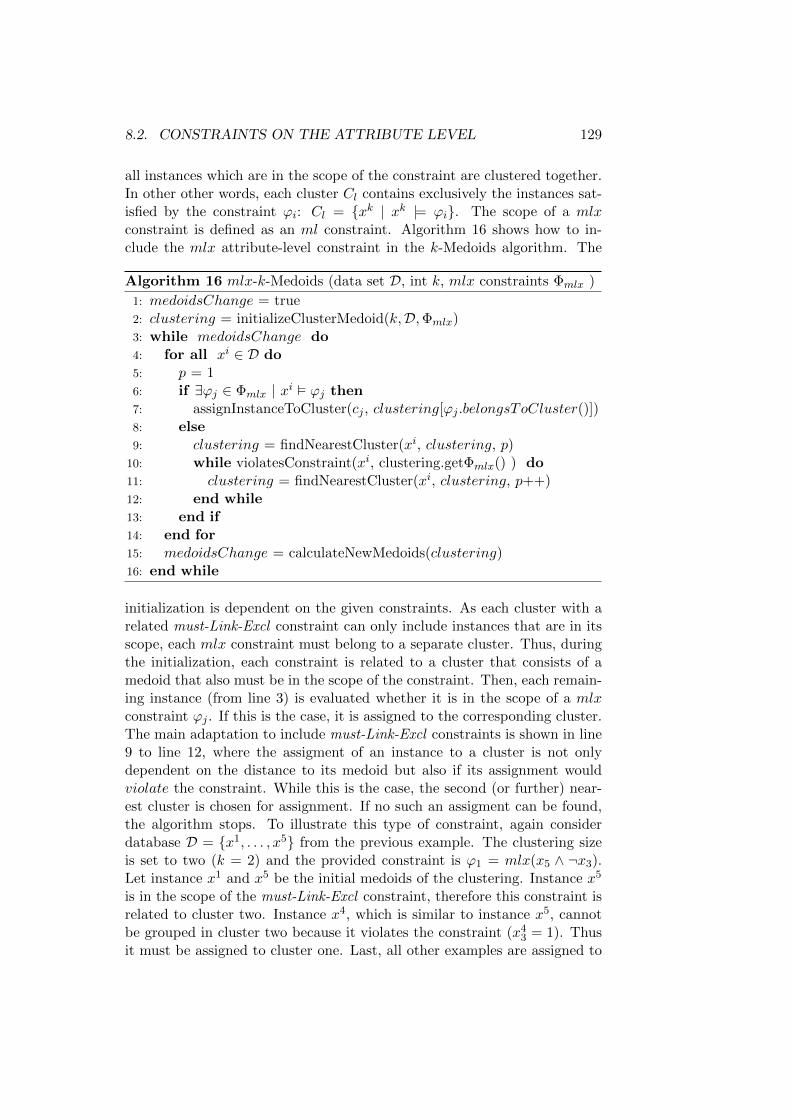
8.2. CONSTRAINTS ON THE ATTRIBUTE LEVEL 129
all instances which are in the scope of the constraint are clustered together.In other other words, each cluster Cl contains exclusively the instances sat-isfied by the constraint ϕi: Cl = {xk | xk |= ϕi}. The scope of a mlxconstraint is defined as an ml constraint. Algorithm 16 shows how to in-clude the mlx attribute-level constraint in the k-Medoids algorithm. The
Algorithm 16 mlx-k-Medoids (data set D, int k, mlx constraints Φmlx )
1: medoidsChange = true2: clustering = initializeClusterMedoid(k,D,Φmlx)3: while medoidsChange do4: for all xi ∈ D do5: p = 16: if ∃ϕj ∈ Φmlx | xi � ϕj then7: assignInstanceToCluster(cj , clustering[ϕj .belongsToCluster()])8: else9: clustering = findNearestCluster(xi, clustering, p)
10: while violatesConstraint(xi, clustering.getΦmlx() ) do11: clustering = findNearestCluster(xi, clustering, p++)12: end while13: end if14: end for15: medoidsChange = calculateNewMedoids(clustering)16: end while
initialization is dependent on the given constraints. As each cluster with arelated must-Link-Excl constraint can only include instances that are in itsscope, each mlx constraint must belong to a separate cluster. Thus, duringthe initialization, each constraint is related to a cluster that consists of amedoid that also must be in the scope of the constraint. Then, each remain-ing instance (from line 3) is evaluated whether it is in the scope of a mlxconstraint ϕj . If this is the case, it is assigned to the corresponding cluster.The main adaptation to include must-Link-Excl constraints is shown in line9 to line 12, where the assigment of an instance to a cluster is not onlydependent on the distance to its medoid but also if its assignment wouldviolate the constraint. While this is the case, the second (or further) near-est cluster is chosen for assignment. If no such an assigment can be found,the algorithm stops. To illustrate this type of constraint, again considerdatabase D = {x1, . . . , x5} from the previous example. The clustering sizeis set to two (k = 2) and the provided constraint is ϕ1 = mlx(x5 ∧ ¬x3).Let instance x1 and x5 be the initial medoids of the clustering. Instance x5
is in the scope of the must-Link-Excl constraint, therefore this constraint isrelated to cluster two. Instance x4, which is similar to instance x5, cannotbe grouped in cluster two because it violates the constraint (x4
3 = 1). Thusit must be assigned to cluster one. Last, all other examples are assigned to

130 CHAPTER 8. ATTRIBUTE CONSTRAINED CLUSTERING
the clusters without considering the constraints because they are not in itsscope. Instance x3 and x2 belong to cluster 1. The resulting clustering C isthus C = {{x1, x2, x3, x4}, {x5}}.
8.2.4 Convergence of Attribute Constrained Clustering
Another question when using this type of attributes is whether the proposedalgorithms terminate. As k-Medoids is proven to converge (condition 1)an evaluation of the inclusion of the ml or mlx constraints is necessary.This can be shown by contradiction: If there is an instance that is in thescope of a constraint ϕi, ϕi is related to the cluster to which the instanceis assigned. If there is no such instance, the constraint is not consideredfor the clustering process. Then, all instances that are also in the scopeof ϕi are as well assigned to this cluster (in the same iteration or at mostone iteration later). Thus for all instances in the scope of ϕi the algorithmalways finds a solution (even in at most two iterations). Moreover, theassignment of theses instances remains fixed for the rest of the clusteringprocess. The remaining instances are clustered via the standard k-Medoidsprocedure. If there was no possibility to find a solution for the remaininginstances, then the standard k-Medoids would not terminate. However, thisis a contradiction to condition 1 and thus, the algorithms must terminate.
8.2.5 Extension of Attribute Constrained Clustering
Although the constraints in this work are defined and applied on binary dataonly, an extension to non-binary data is straightforward. To do so, literals ximean that the value of that variable is in relation to a constant in an instance,whereas a negated literal ¬xi means that the variable is not in relation withthat constant: xl ⇔ xil
⊙c, where c ∈ < and
⊙∈ {<,5,=,=, >}. must-
Link and must-Link-Excl can then be used as described above.
8.3 Experiments
This section first introduces the synthetic datasets that were created forthe experiments. Second, an evaluation measure is presented and last, theexperimental results are shown. For each constraint, the dependency onfour parameters is evaluated: the number of attributes an instance con-sists of (numAttr), the number of attributes that are used in the constraint(numFixedAttr), the number of constraints in the data set (numConstraints)and finally, the number of instances in such a data set (numInstances). Asthis part of the thesis is focused on binary instances, the Hamming distancewas chosen for the clustering process. It captures the proportion of dissim-ilarity between two instances x and y (cf. Equation 8.5), where n01 (n10) is
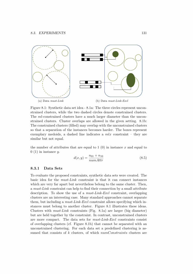
8.3. EXPERIMENTS 131
(a) Data must-Link (b) Data must-Link-Excl
Figure 8.1: Synthetic data set idea - 8.1a: The three circles represent uncon-strained clusters, while the two dashed circles denote constrained clusters.The ml-constrained clusters have a much larger diameter than the uncon-strained clusters. Cluster overlaps are allowed in the given setting. 8.1b:The constrained clusters (filled) may overlap with the unconstrained clustersso that a separation of the instances becomes harder. The boxes representexemplary medoids, a dashed line indicates a mlx constraint – they aresimilar but not equal.
the number of attributes that are equal to 1 (0) in instance x and equal to0 (1) in instance y.
d(x, y) =n01 + n10
numAttr(8.5)
8.3.1 Data Sets
To evaluate the proposed constraints, synthetic data sets were created. Thebasic idea for the must-Link constraint is that it can connect instanceswhich are very far apart but nevertheless belong to the same cluster. Then,a must-Link constraint can help to find their connection by a small attributedescription. To show the use of a must-Link-Excl constraint, overlappingclusters are an interesting case. Many standard approaches cannot separatethem, but including a must-Link-Excl constraint allows specifying which in-stances must belong to another cluster. Figure 8.1 illustrates these ideas.Clusters with must-Link constraints (Fig. 8.1a) are larger (big diameter)but are held together by the constraint. In contrast, unconstrained clustersare more compact. The data sets for must-Link-Excl constraints consistof overlapping clusters (cf. Figure 8.1b) that cannot be separated with anunconstrained clustering. For each data set a predefined clustering is as-sumed that consists of k clusters, of which numConstraints clusters are

132 CHAPTER 8. ATTRIBUTE CONSTRAINED CLUSTERING
Parameter Abbrv Default Min Max
numAttr A 100 20 1000numFixedAttr F 4 1 60numConstraints C 4 1 20numInstances I 1000 40 1000
Table 8.1: Overview of the chosen parameter setting. For each parameter adefault value is given and their ranges, respectively.
constrained. For each unconstrained cluster a medoid of length numAttris created that is at least interMedoidDist apart from the other medoids.The parameter prob gives the probability of ones (xji = 1) in the medoid.Second, numConstraints constrained medoids are created. The parame-ter numFixedAttr defines how many literals are included in the constraint.Next, instances for the unconstrained clusters are generated, by varying themedoid of the corresponding cluster so that they are no more than smallDistapart from their medoid. For constrained clusters, they must not be morethan bigDist apart and moreover, must be in the scope of the constraintthat is related to that cluster. Altogether, numInstances instances areinduced, where a cluster contains on average numInstances (resp. k) in-stances. For the must-Link-Excl constrained clusters, the medoids are notcreated independently like it is the case for must-Link data sets. Instead,the constrained cluster medoids are derived from the unconstrained clustermedoids such that the resulting medoids are similar and the clusters overlap.To examine the quality of the clustering depending on the different ranges ofthe parameters, data sets with different parameter settings were generated.Table 8.3.1 summarizes these parameters’ settings with their default val-ues and the corresponding ranges. Throughout the value of the parametersprob (0.3), smallDist (0.1), bigDist (0.5), interMedoidDist (0.02) and k(20) were left fixed. Altogether, for each constraint (ml, mlx) and parame-ter value, 20 datasets were created, to take into account the variance amongdata sets.
8.3.2 Evaluation of Constrained Clustering
To evaluate the resulting clustering, the Adjusted Rand Index [46] (ARI)is measured. It is an adjusted version of the Rand Index [50] (RI) as de-scribed in section 3.2. A second quality parameter is the change in runtimeand iterations, respectively, when the constraints are incorporated into theclustering process. Due to the ordering dependency and the random initial-ization procedure of the k-Medoids algorithm, each experiment was repeated10 times to eliminate incidental effects. Altogether, this gives 200 test resultsfor each parameter value and constraint.
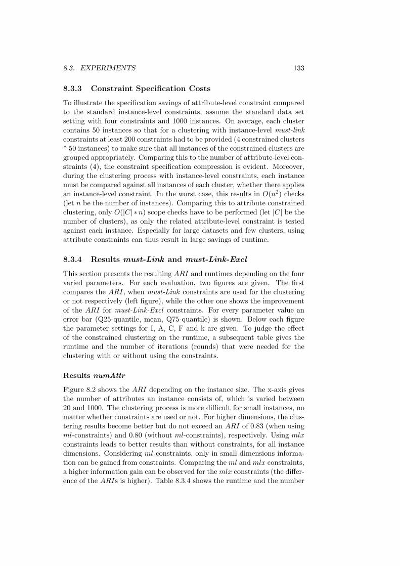
8.3. EXPERIMENTS 133
8.3.3 Constraint Specification Costs
To illustrate the specification savings of attribute-level constraint comparedto the standard instance-level constraints, assume the standard data setsetting with four constraints and 1000 instances. On average, each clustercontains 50 instances so that for a clustering with instance-level must-linkconstraints at least 200 constraints had to be provided (4 constrained clusters* 50 instances) to make sure that all instances of the constrained clusters aregrouped appropriately. Comparing this to the number of attribute-level con-straints (4), the constraint specification compression is evident. Moreover,during the clustering process with instance-level constraints, each instancemust be compared against all instances of each cluster, whether there appliesan instance-level constraint. In the worst case, this results in O(n2) checks(let n be the number of instances). Comparing this to attribute constrainedclustering, only O(|C| ∗n) scope checks have to be performed (let |C| be thenumber of clusters), as only the related attribute-level constraint is testedagainst each instance. Especially for large datasets and few clusters, usingattribute constraints can thus result in large savings of runtime.
8.3.4 Results must-Link and must-Link-Excl
This section presents the resulting ARI and runtimes depending on the fourvaried parameters. For each evaluation, two figures are given. The firstcompares the ARI, when must-Link constraints are used for the clusteringor not respectively (left figure), while the other one shows the improvementof the ARI for must-Link-Excl constraints. For every parameter value anerror bar (Q25-quantile, mean, Q75-quantile) is shown. Below each figurethe parameter settings for I, A, C, F and k are given. To judge the effectof the constrained clustering on the runtime, a subsequent table gives theruntime and the number of iterations (rounds) that were needed for theclustering with or without using the constraints.
Results numAttr
Figure 8.2 shows the ARI depending on the instance size. The x-axis givesthe number of attributes an instance consists of, which is varied between20 and 1000. The clustering process is more difficult for small instances, nomatter whether constraints are used or not. For higher dimensions, the clus-tering results become better but do not exceed an ARI of 0.83 (when usingml-constraints) and 0.80 (without ml-constraints), respectively. Using mlxconstraints leads to better results than without constraints, for all instancedimensions. Considering ml constraints, only in small dimensions informa-tion can be gained from constraints. Comparing the ml and mlx constraints,a higher information gain can be observed for the mlx constraints (the differ-ence of the ARIs is higher). Table 8.3.4 shows the runtime and the number

134 CHAPTER 8. ATTRIBUTE CONSTRAINED CLUSTERING
(a) Comparison must-Link
(b) Comparison must-Link-Excl
Figure 8.2: Resulting ARI for different instance sizes (number of attributes)(I = 1000, A = -, C = 4 , F = 4, k = 20)
of rounds that were needed for the clustering. The larger the instances,the longer needs the clustering. This is mainly due to the longer instancecomparison time, which of course increases for higher dimension. In fact,the clustering becomes easier for higher dimension for ml constraints, be-
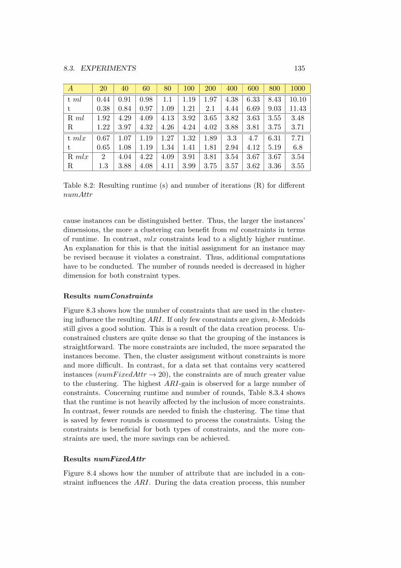
8.3. EXPERIMENTS 135
A 20 40 60 80 100 200 400 600 800 1000
t ml 0.44 0.91 0.98 1.1 1.19 1.97 4.38 6.33 8.43 10.10t 0.38 0.84 0.97 1.09 1.21 2.1 4.44 6.69 9.03 11.43
R ml 1.92 4.29 4.09 4.13 3.92 3.65 3.82 3.63 3.55 3.48R 1.22 3.97 4.32 4.26 4.24 4.02 3.88 3.81 3.75 3.71
t mlx 0.67 1.07 1.19 1.27 1.32 1.89 3.3 4.7 6.31 7.71t 0.65 1.08 1.19 1.34 1.41 1.81 2.94 4.12 5.19 6.8
R mlx 2 4.04 4.22 4.09 3.91 3.81 3.54 3.67 3.67 3.54R 1.3 3.88 4.08 4.11 3.99 3.75 3.57 3.62 3.36 3.55
Table 8.2: Resulting runtime (s) and number of iterations (R) for differentnumAttr
cause instances can be distinguished better. Thus, the larger the instances’dimensions, the more a clustering can benefit from ml constraints in termsof runtime. In contrast, mlx constraints lead to a slightly higher runtime.An explanation for this is that the initial assignment for an instance maybe revised because it violates a constraint. Thus, additional computationshave to be conducted. The number of rounds needed is decreased in higherdimension for both constraint types.
Results numConstraints
Figure 8.3 shows how the number of constraints that are used in the cluster-ing influence the resulting ARI. If only few constraints are given, k-Medoidsstill gives a good solution. This is a result of the data creation process. Un-constrained clusters are quite dense so that the grouping of the instances isstraightforward. The more constraints are included, the more separated theinstances become. Then, the cluster assignment without constraints is moreand more difficult. In contrast, for a data set that contains very scatteredinstances (numFixedAttr → 20), the constraints are of much greater valueto the clustering. The highest ARI-gain is observed for a large number ofconstraints. Concerning runtime and number of rounds, Table 8.3.4 showsthat the runtime is not heavily affected by the inclusion of more constraints.In contrast, fewer rounds are needed to finish the clustering. The time thatis saved by fewer rounds is consumed to process the constraints. Using theconstraints is beneficial for both types of constraints, and the more con-straints are used, the more savings can be achieved.
Results numFixedAttr
Figure 8.4 shows how the number of attribute that are included in a con-straint influences the ARI. During the data creation process, this number

136 CHAPTER 8. ATTRIBUTE CONSTRAINED CLUSTERING
(a) Comparison must-Link
(b) Comparison must-Link-Excl
Figure 8.3: Resulting ARI for clusterings with a different number of con-straints (I = 1000, A = 100, C = - , F = 4, k = 20)

8.3. EXPERIMENTS 137
C 1 2 4 5 7 8 10 11 13 14
t ml 1.16 1.31 1.21 1.21 1.18 1.19 1.2 1.17 1.12 1.13t 1.23 1.28 1.24 1.27 1.23 1.28 1.29 1.23 1.24 1.2
r ml 4.11 3.94 3.9 3.83 3.79 3.67 3.52 3.54 3.42 3.29r 4.22 4.33 4.24 4.42 4.22 4.37 4.29 4.11 4.1 4.09
t mlx 1.38 1.36 1.41 1.37 1.39 1.42 1.32 1.21 1.18 1.18t 1.41 1.41 1.48 1.44 1.45 1.45 1.46 1.46 1.56 1.59
r mlx 4.1 4 3.95 3.92 3.76 3.63 3.54 3.46 3.28 3.12r 4.08 4 4.03 3.92 3.77 3.76 3.67 3.6 3.44 3.45
C 16 17 19 20
t ml 0.99 1 0.89 0.84t 1.23 1.23 1.18 1.15
r ml 3.06 3.02 2.81 2.73r 4.14 4.16 4 3.86
t mlx 1.18 1.14 1.09 0.99t 1.61 1.61 1.61 1.43
r mlx 2.89 2.64 2.44 2r 3.39 3.14 3.15 3.06
Table 8.3: Resulting runtime (s) and number of iterations for differentnumConstraints
specified the similarity of the instances within a cluster, because if an at-tribute is used for a constraint, its value will always be equal for all instancesin the cluster. Overall, the constraints provide some additional informationfor the clustering, which is evident especially for mlx constraints. The bestimprovement can be observed when only few attributes are included in theconstraints. Then, the higher variability in the instances is a problem forthe unconstrained k-Medoids clustering. That is why the most improvementover a standard approach is to be found for small numbers of numFixedAttr.The ARI-gain decreases for higher values of numFixedAttr, because thenthe instances become more and more similar so that k-Medoids is also ableto induce the correct clustering. How the runtime and number of roundsis affected by the inclusion of more attributes in the constraints is pre-sented in Table 8.3.4. For must-Link constraints, the runtime increaseswith higher values of numFixedAttr, no matter whether the constraints areconsidered or not. Here, the unconstrained clustering is even comparablein the runtime. Although the runtime does not increase much for must-Link-Excl constraints, the runtime is also comparable to the case when noconstraints are considered. The number of rounds is the same for all valuesof numFixedAttr, when using constraints, but slightly decreased for thestandard approach. This can be explained by the fact that the separation

138 CHAPTER 8. ATTRIBUTE CONSTRAINED CLUSTERING
(a) Comparison must-Link
(b) Comparison must-Link-Excl
Figure 8.4: Resulting ARI for a different number of attributes that areincluded in a constraint (I = 1000, A = 100, C = 4 , F = -, k = 20)

8.3. EXPERIMENTS 139
F 2 4 6 8 10 15 20 25 30 35
t ml 1.17 1.22 1.21 1.23 1.23 1.21 1.28 1.23 1.24 1.26t 1.19 1.23 1.24 1.22 1.23 1.25 1.24 1.24 1.25 1.27
r ml 3.85 3.86 3.81 3.94 3.98 3.81 3.96 3.92 3.9 3.92r 4.28 4.23 4.26 4.17 4.22 4.21 4.12 4.09 4.1 4.1
t mlx 1.36 1.32 1.34 1.38 1.37 1.34 1.34 1.34 1.36 1.39t 1.42 1.37 1.4 1.37 1.38 1.4 1.39 1.43 1.42 1.48
r mlx 3.85 3.99 4 3.91 3.97 3.94 3.87 3.88 3.9 3.89r 3.97 3.94 3.96 3.91 3.89 3.96 3.92 4.01 3.96 4.07
F 40 45 50 55 60
t ml 1.25 1.29 1.37 1.37 1.39t 1.26 1.3 1.3 1.32 1.34
r ml 3.85 3.78 3.93 3.89 4.03r 4.05 4.05 4 4.09 4.1
t mlx 1.36 1.4 1.42 1.36 1.4t 1.45 1.43 1.43 1.43 1.43
r mlx 3.88 3.84 4.03 3.9 3.92r 4.16 4 4.01 4.12 4.08
Table 8.4: Resulting runtime (s) and number of iterations for differentnumFixedAttr
of the instances becomes easier, because more fixed attributes mean thatthe resulting instances are more similar. Thus, the standard clustering con-verges earlier. However, in most cases the constrained clustering needs fewerrounds than the standard clustering approach.
Results numInstances
Figure 8.5 shows the ARI for differently sized data sets. The data setsinclude from 40 to 4000 instances each. The inclusion of both typesof constraints is beneficial. Throughout the parameter values, an averageimprovement of 4.2% (ml) and 12% (mlx) can be observed. The biggestimprovement was achieved for small data sets (ml: 6.8% and mlx: 15% re-spectively) but no general trend can be inferred from these numbers. Table8.3.4 shows that larger datasets increase the runtime and iterations. Theinclusion of constraints is beneficial for the runtime and rounds. Both arelower when compared to the standard clustering approach.

140 CHAPTER 8. ATTRIBUTE CONSTRAINED CLUSTERING
(a) Comparison must-Link
(b) Comparison must-Link-Excl
Figure 8.5: Resulting ARI for a different number of instances (I = -, A =100, C = 4 , F = 4, k = 20)

8.3. EXPERIMENTS 141
I 40 60 100 200 400 600 800 1000 2000 4000
t ml 0.1 0.15 0.2 0.3 0.58 0.69 0.89 1.2 3.48 13.72t 0.11 0.14 0.2 0.34 0.64 0.75 1 1.29 3.69 14.74
r ml 2.71 3.12 3.44 3.52 3.75 3.84 3.85 3.94 4.01 4.02r 2.81 3.32 3.56 3.9 4.05 4.22 4.37 4.3 4.3 4.26
t mlx 0.1 0.14 0.19 0.31 0.62 0.84 1.07 1.31 3.29 11.87t 0.1 0.14 0.16 0.31 0.6 0.82 1.09 1.37 3.75 14.34
r mlx 2.71 3.16 3.35 3.62 3.69 3.77 3.98 3.88 3.91 3.86r 2.84 3.17 3.41 3.67 3.67 3.87 3.94 3.85 4.08 3.88
Table 8.5: Resulting runtime (s) in second and number of iterations fordifferent numInstances
Results on the Real-World Data Set
A last experiment shows the applicability of the constraints on a real-worlddata set. The UCI zoo data set2 was chosen for this experiment. It con-tains 101 binary instances that describe animals. Additionally, the corre-sponding cluster membership (the biological class) is included. Six con-straints were created using biological background knowledge about the sim-ilarities of animals and the given attributes: ml1(milk), ml2(feathers),ml3(fins ∧ eggs), ml4(4Legs ∧ toothed ∧ eggs ), ml5(6Legs ∧ breathes),ml6(¬backbone ∧ ¬breathes). The same constraints were also created forthe mlx type. Then, sets of constraints were created, including one to sixconstraints each, in order to show the individual contribution for each con-straint as well as the benefit of their combinations. For each possible com-bination, a separate constraint set was constructed and then used for theclustering process. Again, the clustering was repeated 50 times for each con-straint set. Figure 8.6a shows the mean ARI for each constraint set size aswell as the baseline result when no constraints are considered. The leftmostpoint(s) (above 1) give the average ARI when the constraint set consists ofonly one constraint, while the point(s) above 2 show the average ARI forthe combination of two constraints each. The results indicate that the moreconstraints are applied, the better is the clustering quality. However, notevery constraint or constraint combination performs equally well. Figure8.6b gives the mean ARI for each mlx constraint and their combinations.Although the general trend shows that the inclusion of such constraints isbeneficial, there exist constraints (and combinations) that do not improvethe result notably. Especially the inclusion of constraints mlx3 and mlx6
only leads to small improvements. Most significantly, the constraint mlx6
alone even decreases the ARI compared to the baseline (leftmost point in
2http : //archive.ics.uci.edu/ml/datasets/Zoo

142 CHAPTER 8. ATTRIBUTE CONSTRAINED CLUSTERING
(a) Mean ARI for constraint sets
(b) ARI for individual mlx constraint sets
Figure 8.6: ARI for the Zoo data set. (I = 101, A = 23, C = 1-6 , F = 1-3,k = 7)

8.4. CONCLUSION 143
Figure 8.6b). This shows that such constraints (as every other type of con-straints) must be defined very carefully, but may significantly improve theclustering performance.
8.4 Conclusion
In this chapter we transferred the notions of the instance-level constraintsmust-Link and cannot-Link to the attribute level, where the cannot-Linkeffectively becomes a new type of constraint: must-Link-Excl. An adapta-tion of the well-known k-Medoids algorithm was presented that is able toincorporate the provided constraints. Each constraint was evaluated con-cerning several parameters. The results indicate that it is not only possibleto define constraints on the attribute level, but also that they may be verybeneficial in the clustering process. Moreover, we discussed on which typesof clustering problems the constraints should be applied and how much thespecification costs can be reduced compared to standard instance-level con-straints. For future work, we would like to consider the combination of thepresented constraints, how this combination will affect the runtime and howa probably NP-hard problem (like for other constraint clusterers [26]) can beavoided. Moreover, we would like to examine how constraints that express,e.g. the amount of shared attributes between clusters, can be formalizedand incorporated into the constrained mining process.

144 CHAPTER 8. ATTRIBUTE CONSTRAINED CLUSTERING
Chapter 9
An Online Approach forPRTA Induction (OPRTA)
The recent creation of massive time labeled data sets (or event sequences[69]) in all areas of sciences and industry increases the need for scalablemethods that induce models for any kind of underlying processes. Espe-cially models that automatically induce the main elements of such processes(e.g., events) are very interesting for time-cause analyses. Important appli-cation areas include, amongst others, the analysis of disease progressions anddisease patterns [67]. Probabilistic real time automata are a new graphicalmodel to represent such processes. They automatically induce states andtransitions based only on the data set. Moreover, they enable insights intothe temporal relationships [97] and probabilities of change from one state tothe next. The induction of PRTAs is currently based on the state mergingmethod [78], which is considered state of the art in automata induction.However, this also includes the creation of a prefix tree acceptor (PTA) anda subsequent clustering step. For massive data sets both of these steps canbecome very time and memory consuming. Using an online approach is astraightforward solution for this problem and can be solved easily for theclustering step. However, how to achieve the PTA creation is still unknown.We tackle this problem by transforming both steps into online versions [82].Each instance of the data set is first converted into a PRTA, which is thenmerged with a pre-existing one. The merge step is based on a clustering thatuses maximum frequent patterns as representatives. We chose this cluster-ing strategy to identify very homogeneous states, i.e. states that combineevents having the same co-occurring characteristics. Moreover, this enablesthe incremental creation of PRTAs for data streams, which may arise, e.g. insensor networks. The method is also able to deal with concept drift in suchdata streams, i.e. the PRTA is able to detect and to model a shift in theunderlying process by the creation (or deletion) of states and transitions.Similar to existing work [61] this is done if a new event type is detectedor when a state becomes out of date. We show that this method produces
145

146 CHAPTER 9. ONLINE PRTA INDUCTION
stable and informative automata that can be computed in reasonable time.In summary, our contribution is threefold:
1. We propose an online method for PRTA induction (OPRTA) that canbe used for massive data sets.
2. We present adaptations of the method for data sets with concept drift.
3. We show three real world applications of the method along with theinsights that can be gained from the resulting model.
This chapter first defines the problem setting (Section 9.1 ), the model andexplains the online approach, which is extensively evaluated in Section 9.2.
9.1 Online Induction of PRTAs Based on MFPClustering
This section first introduces the problem, which is followed by an informaldescription of the solution. This is then formalized in Section 9.1.3. Last,Section 9.1.4 explains how the proposed method can be used when conceptdrift is present.
9.1.1 Problem Setting
The task is to model a timed language model of data set D. Let D be adatabase of histories Hi: D = {h1, . . . , hn}. A history hi is a sequence oftimed events hi = (~e1, t1) (~e2, t2) . . . (~el, tl). The event sequence is orderedcorresponding to the time label (tj) of the events. Note that the time labelsneed not necessarily form equal intervals, thus a varying amount of timecan pass between successive events. An event ei is a binary vector ~ei =(ai1, ai2, . . . , aij) consisting of j attributes, where aij is equal to one if theattribute was observed in this event.1 Data set D is to be modeled by aprobabilistic real time automaton (PRTA) A PRTA is a directed graph anddefined as follows.
DefinitionA PRTA Γ is a tuple Γ = (Q,
∑, T, S, F ), where
• Q is a finite set of states
• Σ is a finite set of events
• T is a finite set of transitions
• S = Q is the set of start states
• F = Q is the set of final states1This is similar to the notation of itemsets and thus an event can also be regarded as
an itemset.

9.1. ONLINE INDUCTIONOF PRTAS BASEDONMFP CLUSTERING147
Figure 9.1: Example data set
A state qi ∈ Q is a pair 〈Ei, ~fi〉 where Ei is its set of events (Ei = {~ek : ~ek ∈Ci}) and ~fi is an attribute vector called its profile. Σ are all events ~e that areobserved in the input data. A transition t ∈ T is a tuple 〈q, q′, TL, φ, p〉 whereq, q′ ∈ Q are the source and target states, TL = ∆(Ei, Ej) and φ is a delayguard defined by an interval [t1, t2] with t1, t2 ∈ N. p defines a probability p ∈[0, 1] that this transition occurs. A PRTA that is also able to model conceptdrift (denoted by PRTAC) is defined as tuple Γ = (Q,
∑, T, S, F, Z), where
Z gives for each state and transition the number of timesteps that haveelapsed since their last observation: Z = {(o ⊆ Q ∪ T, k ∈ N+)}.
9.1.2 Overview of the Approach
In this section, the general procedure of how to induce PRTAs online is given.The main idea of the online induction is that each new history is addedincrementally to the existing PRTA. The histories hi ∈ H are observed oneby one. First, each history hi is transformed into a ‘path’-PRTA, wherethere is only one predecessor and one successor for each node (exactly theevents that occurred in the history). This PRTA is then collapsed into aPRTA Γ, i.e. all nodes nl ∈ Q sharing the same profile are merged intoone state. Then, each state nl of Γ is compared to the states Q′ of a pre-existing PRTA Γ′ that is built from all previous histories hl(l < i). If nodenl belongs to state qj ∈ Q′, then node nl is merged with state qj . Thefunction fNN that identifies such a state qj is described in Section 9.1.3.Such a merge also induces that all incoming transitions from state qj areincorporated into Γ′. If the sucessor node nl+1 of nl of the PRTA Γ isalso merged with a state qj+1 of the PRTA, then the transition tn is linkedbetween qj and qj+1. If there is already a transition ts, then it is updatedwith the information of tn. However, if there is no state qj of Γ′ that statenl belongs to, nl is only added to Q′. This also induces that there may be notransition from nl to the remaining states of Q′. To clarify this procedure,consider the following example. Figure 9.1 shows a set of histories consistingof events {α, β, γ, δ, ε, λ, ν, ξ, o}. As the histories are observed one by one,history h1 is considered first. Figure 9.2 illustrates this process. First, the

148 CHAPTER 9. ONLINE PRTA INDUCTION
Figure 9.2: Example for the online induction of a PRTA. Left: Subsequentcollapsed histories (Γ). Right: Resulting automaton (Γ′) when merged withnew collapsed history (Γ)
history h1 is transformed into a PRTA Γ1 (the figure does not illustrate thetransformation of the history in the path automaton), which is followed bythe collapse step: all nodes of h1 having the same profile ~f are merged, whichresults in Γ1. The last step is to find similar nodes in the pre-existing PRTA.As there is no existing automaton for the first instance, Γ1 is equal to Γ′1.Then, the processing of h1 is finished and history h2 can be incorporatedinto the PRTA. Again, the compression is the first step, but cannot beconducted as there are no identical nodes in the history. Thus, Γ2 remainsa sequence of states. Then, each state of Γ2 is compared to Γ′1 whetherthere is a state qj it belongs to. This is true for the states that correspondto the events λ, γ and α: α ∈ Γ2 belongs to state α ∈ Γ′1, because theyhave the same profile, which is also true for γ ∈ Γ2 and γ ∈ Γ′1; λ ∈ Γ2
belongs to state β ∈ Γ′1 because they have a similar profile. (In Figure9.2, the corresponding states of Γ2 and Γ′1 are shaded equally.) The laststep is then to merge the states of Γ2 with the states of Γ′1, resulting inan updated PRTA Γ′2: all states in Γ2 that do not have a correspondingstate in Γ′1 are added to Γ′1, including all their transitions. The others aremerged including their transitions. E.g., transition t′ = 〈β, γ, T ′L, φ′, p′〉 ofthe PRTA Γ′1 and transition t = 〈λ, γ, TL, φ, p〉 of the PRTA Γ2 are mergedto a final transition t′′ = 〈β, γ, T ′′L, φ′′, p′′〉 in the PRTA Γ′2. The state βthen contains two events β and λ, but is still labeled with β, because weassume that λ ≺ β. Moreover, the delay guard φ and the probability p of
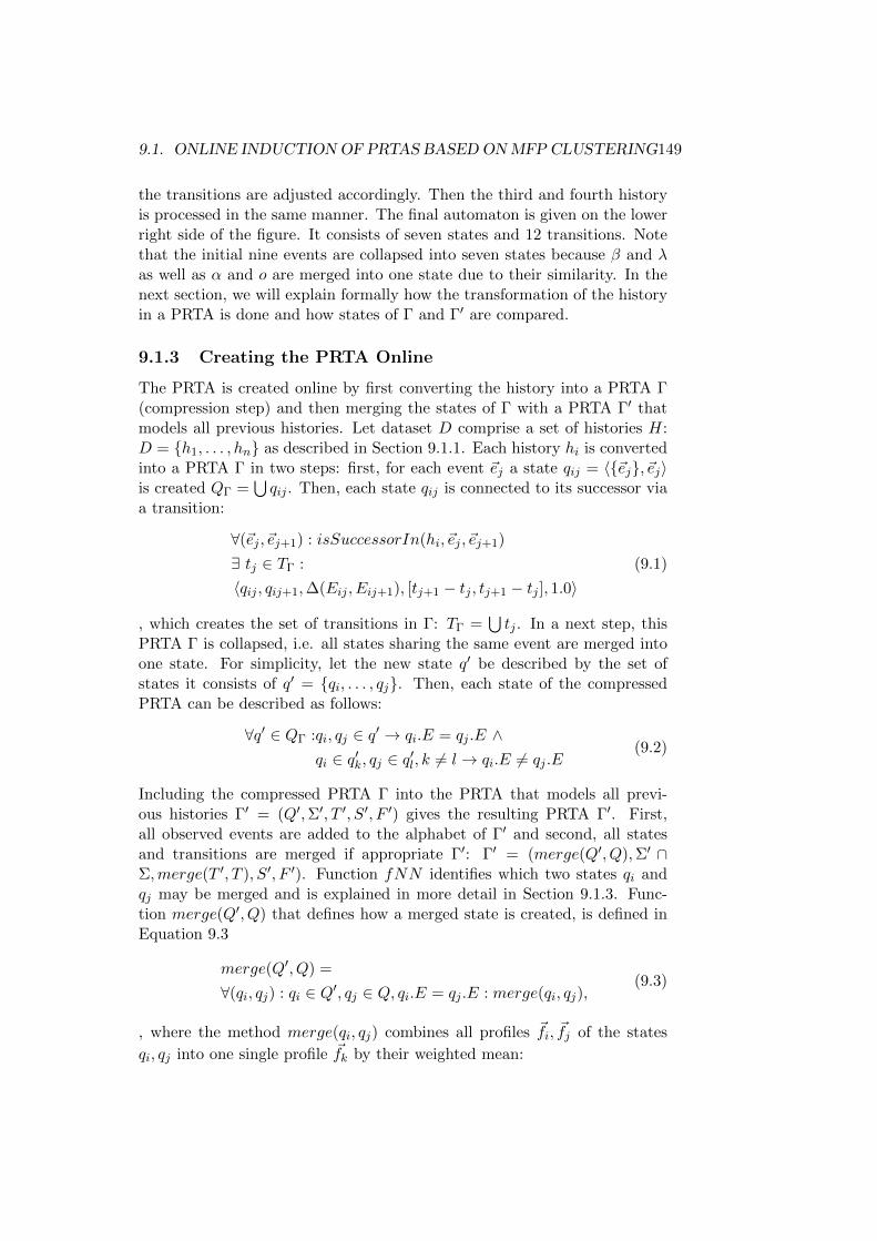
9.1. ONLINE INDUCTIONOF PRTAS BASEDONMFP CLUSTERING149
the transitions are adjusted accordingly. Then the third and fourth historyis processed in the same manner. The final automaton is given on the lowerright side of the figure. It consists of seven states and 12 transitions. Notethat the initial nine events are collapsed into seven states because β and λas well as α and o are merged into one state due to their similarity. In thenext section, we will explain formally how the transformation of the historyin a PRTA is done and how states of Γ and Γ′ are compared.
9.1.3 Creating the PRTA Online
The PRTA is created online by first converting the history into a PRTA Γ(compression step) and then merging the states of Γ with a PRTA Γ′ thatmodels all previous histories. Let dataset D comprise a set of histories H:D = {h1, . . . , hn} as described in Section 9.1.1. Each history hi is convertedinto a PRTA Γ in two steps: first, for each event ~ej a state qij = 〈{~ej}, ~ej〉is created QΓ =
⋃qij . Then, each state qij is connected to its successor via
a transition:
∀(~ej , ~ej+1) : isSuccessorIn(hi, ~ej , ~ej+1)
∃ tj ∈ TΓ :
〈qij , qij+1,∆(Eij , Eij+1), [tj+1 − tj , tj+1 − tj ], 1.0〉(9.1)
, which creates the set of transitions in Γ: TΓ =⋃tj . In a next step, this
PRTA Γ is collapsed, i.e. all states sharing the same event are merged intoone state. For simplicity, let the new state q′ be described by the set ofstates it consists of q′ = {qi, . . . , qj}. Then, each state of the compressedPRTA can be described as follows:
∀q′ ∈ QΓ :qi, qj ∈ q′ → qi.E = qj .E ∧qi ∈ q′k, qj ∈ q′l, k 6= l→ qi.E 6= qj .E
(9.2)
Including the compressed PRTA Γ into the PRTA that models all previ-ous histories Γ′ = (Q′,Σ′, T ′, S′, F ′) gives the resulting PRTA Γ′. First,all observed events are added to the alphabet of Γ′ and second, all statesand transitions are merged if appropriate Γ′: Γ′ = (merge(Q′, Q),Σ′ ∩Σ,merge(T ′, T ), S′, F ′). Function fNN identifies which two states qi andqj may be merged and is explained in more detail in Section 9.1.3. Func-tion merge(Q′, Q) that defines how a merged state is created, is defined inEquation 9.3
merge(Q′, Q) =
∀(qi, qj) : qi ∈ Q′, qj ∈ Q, qi.E = qj .E : merge(qi, qj),(9.3)
, where the method merge(qi, qj) combines all profiles ~fi, ~fj of the states
qi, qj into one single profile ~fk by their weighted mean:

150 CHAPTER 9. ONLINE PRTA INDUCTION
~fk =1∑
qi∈Q∩Q′ |Ei|∑
qi∈Q∩Q′
|Ei| × ~fi
The merge of the states also induces the merge of transitions, if appropriate.Last, the automaton can also be applied to data sets with concept drift.Here, elements of the automaton may become out of date. Therefore, thelist Z is updated for each event in the history hi: let z ∈ Z be (k, q), wherek is a timepoint and q is a set of states:
∀ (~eij , tij) ∈ hi :
∃ z = (k, q) : k = ti ∧ @ z′ = (k′, q′) : ~eij ∈ q′, k′ > k
→ z = k, q ∪ ~eij(9.4)
Thus, the most recent timepoint is kept for each event and the correspondingstates. Last, all states that exceed the minimum time constraint are deletedfrom the PRTA Γ′′.
∀ q ∈ Q′′ :∃ z = (k, q) : qi ∈ q ∧ k ≥ minTime→ Q = Q\qi, T = T\t :
t = 〈qi, qj , TL, φ, p〉 ∨ t = 〈qj , qi, TL, φ, p〉
(9.5)
Algorithm 17 summarizes this procedure: For each history, a PRTA is cre-ated and compressed. Then, each state of this PRTA may be merged with astate of the pre-existing PRTA. Last, if concept drift is taken into account,the timelist is updated and outdated states and transitions are deleted fromthe PRTA.The time complexity of this approach is a sum of the collapse step and theclustering step. In the worst case O(n2) comparisons must be performedto check whether a state of history hi can be merged with another state ofhistory hi. Next, for each state of Γ, the most similar state in Γ′ is retrieved,which costs O(n ∗m). Therefore, the total complexity of the algorithm isO(n2 + n ∗m).
Function fNN
Function fNN identifies whether there is a state q that is similar to a stateqij in history hi. This is the case if qij covers a large fraction of the frequentpatterns of state q. The identification of frequent shared properties (corre-sponding to the minimum support threshold ms) is achieved by comparing qto the set of maximal frequent patterns (MFPs) of all nodes in qij . This setis updated incrementally via the AIST data structure (cf. Chapter 6)[76].Function fNN computes the fraction of shared properties between q and qijof history hi. If the maximal fraction exceeds a minimum overlap threshold,qij is merged with state q.

9.1. ONLINE INDUCTIONOF PRTAS BASEDONMFP CLUSTERING151
Algorithm 17 InducePRTA (D, minsup ∈ [0, 1], minTime ∈ N,ConceptDrift ∈ {0, 1})
1: Γ′ = (Q = {},Σ{}, T = {}, S = {}, F = {}, Z = {})2: for all hi ∈ H do3: PRTA Γ = createPRTA(hi) // cf. Equation 9.14: Γ = compressPRTA (Γ) // cf. Equation 9.25: for all qij ∈ hi do6: State q = fNN(qij , Q, minsup) // cf. Sec. 9.1.37: if q 6= {} then8: Γ′ = merge(Γ′,q, qij) // cf. Equation 9.39: end if
10: end for11: if ConceptDrift then12: Z = updateTimeList(hi) // cf. Equation 9.413: Γ′ = deleteOldNodes(Z, minTime) // cf. Eq. 9.514: end if15: end for
9.1.4 Adaptation For an Unbounded Data Set With ConceptDrift
The presented algorithm can be adapted for unbounded data streams withconcept drift. Concept drift means that the underlying true concept (hereassumed as an automaton) changes as time goes by and thus, elements of theautomaton become out of date. In the following section the characteristicsof such a data stream setting are described. Moreover, the definition of whenan element of an automaton is out of date will be introduced.
The Repeated World Data Stream Setting
The basic question is how a change of a concept can be observed, where oneessential element is how time is monitored. Often, processes are recordedin successive time intervals. Then, a data bag is created with these mea-surements. In the current problem setting, such a bag is a set of historieswhich is additionally labeled with a time stamp. Such measurements arerepeated in equal intervals, which explain the term repeated world setting.As an example, consider the monitoring of a multivariate process of a com-pany within one week, where at the end of the week the set of histories iscollected and transferred. Then, an updated model can be learned with thisdata bag. In the repeated world setting, concept drift is observed, whenelements of the automaton do no longer occur in recent bags but only inolder ones. Of course, there may also be new elements of an automaton.This may be the case, e.g. if a process changed within the company (maybedue to a change in the personnel). Then some states or transitions may dis-

152 CHAPTER 9. ONLINE PRTA INDUCTION
Figure 9.3: Illustration of the data stream (repeated world) setting. Left:data stream illustration (bags). Right: Resulting automata for the datastream. Added and deleted elements of the automaton are drawn withdashed lines.
appear, while others arise. Thus, the change of the automaton reflects howwhole processes change over time. In the repeated world, the updates of theautomaton are based on the new bags of histories (left part of Figure 9.3).The first important property is that each history in each bag may begin attimepoint t0, i.e. the first event was observed at timepoint t0. This alsosuggests that there exist two timelines. One is the ordering of the events(horizontal timeline) within one history, the second timeline shows in whichorder the bags arrive (vertical timeline). This also defines the time thresholdo when an element is out of date. This is the case, when an event was lastobserved too long ago. As an example consider state 7. This state doesoccur in bag one but not in bag two. Thus, it is out of date when bag 3is observed (o being set to 1) and is therefore deleted. This shows that thetime to evaluate whether one state is out of date is dependent on the timeof the bag and not the timestamp in the history.

9.1. ONLINE INDUCTIONOF PRTAS BASEDONMFP CLUSTERING153
Figure 9.4: Continuous world setting
The Continuous World Data Stream Setting
However, a change of the concept can be observed in another way, when oneset of histories is monitored continuously. There, the set of histories is knownup-front but it is unknown, which history will be updated with the next dataset and how many new events a history will provide. Such a world is thencalled continuous world. As an example for such a world consider the ongoingrecording of fixed population of patients, where each patient record (and sohis history) is extended with each physicians visit. In such a world, a changeof the concept is observed, if there are elements of the automaton that havenot been observed for a long time within all histories. The last observationis the last absolute time point of any history for this element. Note that theset of updates of the histories may also vary in its length. It may containonly the observations for the next timepoint in line, but it also can containupdates over several timepoints. Figure 9.4 shows the continuous worldsetting. In the continuous world, time is measured absolutely, i.e. the timestamp for each event is equal to its last observation within the whole dataset. As the data stream progresses, updates for histories are delivered (e.g.,for H3), or new histories are started (e.g., for H7). For example, the lastobservation for state 7 of the automaton is t1. As more and more data is

154 CHAPTER 9. ONLINE PRTA INDUCTION
recorded, state 7 is not observed anymore and thus is out of date at timepoint t2. Therefore, it is removed from the automaton. The same is true fortransition q1 → q1 (not illustrated in the histories). As time progresses, anew state 7∗ (indicated by dashed circles) is observed and also included inthe data set. Note that these are updates and thus there is only one timeline and the time stamp always increase.
Algorithmic Adjustments
To adapt the presented algorithm for concept drift, each element (states andtransitions) of the automaton must be annotated with a label that showswhen this element was observed the last time. If such an element then be-comes out of date, it must be deleted from the automaton. How this isachieved in detail is presented in the following.
Repeated World Adjustments Beginning with the automaton that is(also incrementally) created with a first bag of histories, the algorithm re-ceives updates of histories (bags) as input. Thus, each update comes alongwith a label that defines the current time stamp. In the repeated world,histories are loaded in bags and processed like in the standard incrementalsetting. Additionally, each element of the automaton is assigned a time-stamp that defines when it was observed the last time: A PRTA that is alsoable to model concept drift is defined as tuple Γ = (Q,
∑, T, S, F, Z) (cf.
Section 9.1.1), where Z is a mapping that gives for each state and transi-tion the number of timesteps that have elapsed since their last observation:Z = {(o ∈ Q ∪ T, k ∈ N+)}. The timepoint is the timestamp of the bagand not the timestamp of the history because the change of the whole pro-cess shall be explored. Each history update is integrated as described aboveinto the existing automaton. Additionally, the last observation timepointof the elements (state or transition) which are covered during the integra-tion process is updated to the current bag timepoint. This is achieved by asimple hash structure. After all histories of the bag are processed, outdatedelements are deleted from the automaton. This is the case if the element’stime stamp is too old compared to the current bag’s time stamp. Note thatthe threshold o, when an element is out of date, is specified by the user.
Continuous World Adjustments Beginning with the automaton thatis created (also incrementally) with a first set of histories, the algorithmreceives updates of specific histories as input: For each history the set ofnewly observed events is given as input. This includes that the last eventof the history is the first event of the history-update so that the startingpoint for each history can be deduced. Each history-update is integratedas described before into the existing automaton. Additionally, each element

9.2. EXPERIMENTS 155
(state or transition) that is covered during the integration process is up-dated to the most recent element observation time point. After each historyupdate was processed, outdated elements are again deleted from the au-tomaton. However, if the data source cannot store the last event of eachhistory, the implementation of this setting may be expensive. Then, thisassignment must be done within the automaton’s structure. Therefore, wedo not concentrate on this setting in the experimental section but only onthe repeated world setting.
9.2 Experiments
This section presents stability results, the performance on real world datasets and finally shows how the algorithms works on a data set with conceptdrift.
9.2.1 Performance on Stream Setting Without Concept Drift
This section addresses the algorithm’s stability, which will be tested onthe synthetic data set and then shown on real world data sets. For thestability experiments, first, a bootstrap analysis presents how often the trueunderlying structure of the automaton is rediscovered. Second, we show howthe size of the histories influences these results. Last, we present how theruntime of the algorithm and the final number of states depends on the threestandard parameters input data size, history length and minimum support.To show the applicability of such a model, we applied the algorithm onseveral real world data sets. Note that we will not address the quality of theclustering because this was already evaluated in Chapter 5.
Stability Analysis
This section shows the results of the experiment in a bootstrap evaluation.The task is to extract the correct structure of a predefined automaton (cf.Section 3.1.1). To compare the final automaton to the predefined one, themeasures ∆States, LStates and the F -Measure, introduced in Section 3.2, aretaken into account.
Rediscovery of a Known Automaton The results of the bootstrapanalysis for the synthetic data set indicate that the proposed solution isable to find the correct number of states and transitions although it tendsto create to many states (cf. Figure 9.5b). Additionally, the distance fromthe induced states to their closest original is also very small (cf. Figure9.5d). Comparing these results to the PRTA induction with a previousPTA-creation 5 (Figures 9.5a to 9.5e), a minimal performance decrease canbe observed, which is owed to the fact that not all events are observable right

156 CHAPTER 9. ONLINE PRTA INDUCTION
●●●●●●●●●●●●●●
●●●●●●●
●●
●●●●●●
●
●●●●
●●●
●●
●
●●●●●
●
●
●
●●
●
●●
●●
●● ●●●
●
●●●●●
●
●
●
●●
●●●●
●
●
●
●●●●●●●
●●
●●●
●
●●●●●●●●●●●●●●●
●
●
●
●●●●●
●
●●●●●●
●
●● ●●●
●
●
●
●
●
●
●● ●
●
●
●
●●●●●●●
●
●●●●●
●
●●●●●
●
●●●●●
●
●●
●
●●
●
●●
●●
●
●
●●●
●
●●●
●●●●●●●
●●●
●●●
●●●●
●
●
●●●
●
●
●●●
●
●●●●
●
●
●
●
●●●●
●●●●
●
●
●
●
●
●●
●
●●●
●●●●
●
●●
●
●
●
●●●
●
●●●●●●●●●●●
●●
●
●
●●
●
●●●●●●●●●●●●●●●
●
●●
●
●
●●●●
●
●
●
●
●
●
●●●●●●●●●●
●
●●
●●●●●●●
●
●
●
●
●●
●
●
●
●●●●●● ●●
●
●
●
●
●●
●
●●●●●●●●
●
●
●
●
●●
●
●●●●●●
●
●●●●●
●
●
●
●●●●●●●
−8
−6
−4
−2
02
4
sampling with replacementpercentage sampled
diffe
renc
e in
sta
tes
0 10 20 30 40 50 60 70 80 90 100
(a) ∆States
●●●
●
●●●●
●
●
●
●●
●●●●●●
●
●
●●
●●
●
● ●●●●●●
●
●●
●
●●●●●●●●
●
●●●
●●
●
●●
●●
●
●●
●●●
●
●●
●
●
●●
●
●
●
●
●●●
●
●
●●●
●●
●
●
●●
●
●
●
●●
●
●
●●
●
●
●
●
●●
●●
●
●
●●●
●
●
●●
●
●●
●
●●●
●●●
●
●
●
●●
●
●●●●
●
●●●●●
●
●
●●
●
●
●●●●
●
●
●
●
●●●
●
●●
●●
●
●●●
●
●
●●●
●●●●
●
●
●●
●
●
●●●●
●
●
●●
●
●
●
●
●●●
●
●
●
●
●●●●
●
●
●●●
●●
●
●●
●
●
●
●●●
●
●
●●
●
●
●●●●
●
●
●●●●●●
●
●
●
●
●
●
●●
●
●
●●●●
●
●
●
●
●●
●
●●
●●●
●●●
●
●●●●
●
●●
●●
●●●●●●
●
●●●
●
●
●
●●
●●
●●●
●
●
●
●●●●●●
●●●
●
●
●
●●
●●
●●
●●●●
●
●
●●●
●
●
●
●●●
●●
●●
●●●
●
●
●●●
●
●●
●●
●
●
●
●
●
●
●
●
●●●●●
●
●●●●●
●
●●●●●●●
●
●●
●●
●
●
●●●●●●●
●
●●●●●●
●●
●●
●
●●●●●●●●●●
●
●
●●●
●
●●
●
●●
●
●
●
●
●●●●● ●
●
●
●●●
●
●
●
●
●●●● ●●
●
●
●
●●●●
●
●●
●●●●●●●●●●●●●●●●●●●●
●
●●●●● ●●●●●●●●●●●
●●
●
●●●●●
●
●●●●●●●
●
●●●●●
●
●
●
●●●●●●●●●●●●●
●
●
●
●●●●●●●
●
●
−8
−6
−4
−2
02
4
sampling with replacementpercentage sampled
diffe
renc
e in
sta
tes
0 10 20 30 40 50 60 70 80 90 100
(b) ∆States
0.0
0.5
1.0
1.5
2.0
2.5
3.0
sampling with replacementpercentage sampled
eucl
idea
n di
stan
ce to
orig
inal
sta
tes
0 10 20 30 40 50 60 70 80 90 100
(c) LStates
0.0
0.5
1.0
1.5
2.0
2.5
sampling with replacementpercentage sampled
eucl
idea
n di
stan
ce to
orig
inal
sta
tes
0 10 20 30 40 50 60 70 80 90 100
(d) LStates
F−Measure
Fre
quen
cy
0.6 0.7 0.8 0.9 1.0
020
4060
8010
012
014
0
(e) F-Measure of learned transitions
F−Measure
Fre
quen
cy
0.55 0.60 0.65 0.70 0.75 0.80 0.85 0.90
050
100
150
(f) F-Measure of learned transitions
Figure 9.5: Accuracy of the induced PRTA compared to an approach usinga PTA [76]. Figures 9.5a - 9.5e show the results when including a previousPTA construction, Figures 5.7b - 5.7f show the results for the proposedapproach.

9.2. EXPERIMENTS 157
History length (ds = 10000) Data set size (hl = 100)
hl runtime #states ds runtime #states
10 3.9 21.5 100 0.96 12.550 10.8 23.6 1000 2.96 18.9
100 21.1 25.6 5000 10.17 22.7500 137.8 28.0 10000 20.96 25.6
1000 419.5 30.3 50000 191.76 26.5100000 725.27 29.9
Table 9.1: Runtime (sec) and number of states for different history lengthsand data set sizes
at the beginning and thus, the online approach is introducing errors at thebeginning. Overall, the accuracy loss compared to an approach that uses aPTA creation are almost negligible. In contrast, the online approach is ableto include more information than the batch approach and may thus producemuch more specific profiles and more accurate transition probabilities. Afurther investigation concerning the RR of a state shows that all states arelearned well except state 7 (not illustrated). This may be due to the smalltransition probability from state 6 to state 7 and its high similarity to state2, so that the events of this state are only rarely observed, or often misplacedin a wrong cluster.
Influence of the History Length We repeated the bootstrap analysisto evaluate the influence of the history length (hl) on the number of finalstates and their profiles’ accuracy. Therefore, data sets having differenthistory lengths (100, 1000, 10000) have been used. Figure 9.6 illustratesthat the longer the histories, the better the induced profiles match those ofthe original automaton. However, this comes along with many more states(cf. Figure 9.6a). This can be explained by more exceptions that are presentin the data for longer histories.
Number of States and Runtime Depending on History Length,Minimum Support and Data Set Size The next evaluation addressesthe algorithm’s dependency on its main parameters: data set size ds, mini-mum support ms and history length (hl). We calculate the runtime and finalnumber of states for 10 different data sets of the synthetic automaton foreach value of hl, ds and ms. The standard parameter values are ms = 0.5,hl = 100 an ds = 10000. Table 9.1 gives the final average number of statesand runtime (in sec) for different values of hl and ds, while Figure 9.7 illus-trates the behavior for various minimum supports over all data sets. Table9.1 shows that the actual runtime is linearly dependent on hl and also nearlylinear with increasing ds. For both parameters, the number of final states

158 CHAPTER 9. ONLINE PRTA INDUCTION
0
10
20
30
40
50
Sampling with replacementPercentage sampled
Euc
lidea
n di
stan
ce to
orig
inal
sta
tes
5 15 25 35 45 55 65 75 85 95
(a) ∆States for all history lengths
0.0
0.1
0.2
0.3
0.4
0.5
0.6
Sampling with replacementPercentage sampled
Euc
lidea
n di
stan
ce to
orig
inal
sta
tes
5 15 25 35 45 55 65 75 85 95
(b) LStates for all history lengths
Figure 9.6: Stability of the online algorithm for the proposed approach((yellow, green, blue): hl = (100, 1000, 10000)) Difference of states (Top)and Euclidean distance (Bottom) for the induced automaton to the trueautomaton structure.

9.2. EXPERIMENTS 159
15
20
25
30
Minimum Support
Run
time
(gre
en)
and
Num
ber
of S
tate
s (g
old)
0.1 0.2 0.3 0.4 0.5 0.6 0.7 0.8 0.9
Figure 9.7: Number of final states (yellow) in the automaton and the corre-sponding average runtime in sec (green) for a varying minimum support.
increases, which is to be expected as the more data is present, the moreexceptions (and thus new patterns) occur. For such exceptions new statesare created. However, the final number of states is quite small comparedto the number of events in the data set (10,000,000), which shows that thealgorithm can compress the patterns in the data. Figure 9.7 illustrates thatthe runtime is quite stable with different numbers of ms, while the numberof final states decreases. This can be explained by the fact that if the min-imum support increases, more and more instances in a cluster must coverthe representative pattern. This can only be achieved if the representativepattern is small. Then, more instances cover this pattern and are added tothe cluster. Therefore, fewer clusters are found.
Runtime Comparison of the Approach To illustrate the advantagesof the genuine online approach, we compared its runtime (cf. Table 9.1) tothe approach that first creates a PTA and subsequently runs the proposedonline clustering (cf. Chapter 5)[76]. Such an approach needs 2,6 s onaverage (hl = 100) for ds = 100, 333 s for ds = 1000 and already 9 hours fords = 5000. This extreme difference is mainly due to the merging procedure,which takes very long. However, even the creation of the histories, the PTAand the subsequent clustering lasts approximately 17 s, which is still abovethe runtime of the online approach.

160 CHAPTER 9. ONLINE PRTA INDUCTION
Hepatitis data set
ds 50 100 200 400 600 900 1K 1236
s 6 11 18 37 54 75 81 90
Disease group data set
ds 100 1K 5K 10K 50K 100K 147656
s 1 1 2 2 8 24 51
Table 9.2: Runtime (sec) on the Hepatitis data set for different data setsizes (ds)
Performance on the Real World Data Sets
This section presents results of the proposed method for real world medicaland biological data sets. Therefore, the Hepatitis, disease group and yeastdata set have been used and their results are now discussed consecutively.First, the runtime of the approach is tested on the Hepatitis data set. Table9.2 gives the results and shows that even for such a ‘hard’ (because it has alot of attributes and long histories) data set, the runtime is reasonably low.Note that although the number of instances is only 1236, this Hepatitis dataset includes 52,520 single events, due to the long histories. The main timeconsuming step here is the clustering and not the collapse method. The re-sulting automaton can be used to foresee how the blood values will developbased on the current blood values.The same evaluation was run for the first disease group data set (P10), forwhich the runtime is also shown in Table 9.2 (lower part). Here, the algo-rithm is faster as there are less attributes and shorter histories given. Again,the runtime is reasonable for the given application. Interestingly, the algo-rithm identifies a stable number of states (52) for data sets with more than5000 histories. When applying our approach on the second disease groupdata set (P01), the resulting automaton identifies 181 states within a totalruntime of about 2 minutes. This shows that even with a larger number ofattributes, the approach is still fast. Moreover, the number of states doesalso not increase for data sets larger than 5000 histories. The stable num-ber of states for both data sets suggests that all important patterns in thedata have been found. Although the final number of transitions increasesfor larger data sets, the ratio of new transitions decreases. We thus canexpect that even the number of transitions will be fixed at a certain dataset size. PRTA learning based on DIANA clustering [76] is not included inthis comparison as even for the smallest data set it runs out of memory andneeds longer than the online approach on the largest data set.Regarding the structural properties of the resulting automaton for data setP10, we observe that most states have short representatives (MFPs): mostly,they consist of one to three DGs. The full profile then comprises the repre-

9.2. EXPERIMENTS 161
sentative DGs and may additionally have exceptional DGs. 20% of the statescover more than 50 events, while about the same amount captures less than5 events. There are no states with no in/outgoing transitions except twostates, which shows that different disease phases of different persons havebeen well combined in the automaton. Thus, the automaton is a generaliza-tion of the individual patient histories. There are also several hubs, whichcombine events that share very frequent DGs. Moreover, plenty of excep-tional DGs are found in the profiles of the hubs. Such a state reflects veryfrequent disease phases along with all possible comorbidities. However, theadditional diseases may be regarded as random side effects as their do notoccur as often as the main disease. Overall, many states focus on the DGshypertension, diabetes or heart problems, i.e. these DGs have a frequencyof more than 90% in the resulting profile. This makes sense in a way asthese are also the most common diseases, which are then represented alongwith their accompanying diseases. The transitions in this automaton reflectthe probability of a change in the disease status, i.e. whether new diseasesarise or others are cured or not coded anymore. For the most hubs there isno one main transition, but several having a moderate probability. Non-hubstates, in contrast, are associated with such a main transition but this canstill be regarded as a random effect, because there are not so many patienthistories included. Overall, the automaton shows which disease patternsexist in this specific population and how probable transitions from one toanother disease status can be.The last experiment addresses the biological knowledge that can be inferredfrom such an automaton. Figure 9.8 is the final automaton for the yeast dataset. The states’ profiles show which gene is active at which timepoint andtherefore, the metabolism of the cell. The overall structure of the automatonshows that the cell in this experiment undergoes a cycle in the gene expres-sion. This is known to be the cell cycle. Besides, a known resting phase ismodeled by the delay guard (ϕ = [1, 2]) on transition 1 to 2 that shows thatthe cell can either step forward to the very next cell stage or wait. All theseexperiments show that a PRTA can correctly identify the stages of life in apopulation or of individuals, annotate them with important properties andcan thus reflect the dynamics in such systems.
9.2.2 Performance on Stream Setting With Concept Drift
Finally, the approach is tested in a setting with concept drift. Therefore,we created a data set that is based on three different underlying automatathat are derived from the one shown in Figure 3.1. This illustrates therepeated world (cf. Section 9.1.4) setting, where after a certain time spanthe underlying process changes, i.e. different automata should be found. Thefirst automaton is the standard automaton. For the second one (the secondconcept), state 7 was deleted as well as transitions 1 → 1 and 3 → 4. The

162 CHAPTER 9. ONLINE PRTA INDUCTION
Figure 9.8: Result of the approach on the yeast data set. The black andwhite squares represent the values of the genes in the state’s profile. Thedarker, the higher its values.
ds 100 500 1000 5000 10000 50000 100000
s 1 2.3 3.4 11 23 202 745
Table 9.3: Mean runtime (in seconds) for the data set including conceptdrift for different data set sizes (ds)
second derived automaton (concept three) includes a state 7∗ with profile[4,8] and additional transitions. Using these concepts, the first bag of thedata set is created by using the original automaton, the second and thethird bag with the first and second derived automaton (cf. Figure 9.3,right). Then, the algorithm was applied with o = 1 (cf. Section 9.1.4). Theconcept changes are well identified for small error ratios (not illustrated).As for larger error ratios the clustering is also harder, the quality of theinferred automata decreases. Table 9.3 shows how the search for conceptdrift affects the runtime. The runtime is only slightly longer than for theapproach that does not account for concept drift. We thus can concludethat the approach may also be valuable for problems with concept drift.
9.3 Conclusion
In this chapter, we introduced a method to induce PRTAs online. Therefore,we leave out the PTA construction step and instead collapse the histories

9.3. CONCLUSION 163
before merging them with a pre-existing PRTA. Still, this merging is basedon an online clustering method. Besides, we discuss how this approach canhandle data streams with concept drift. The experiments on synthetic andreal world data sets showed that the method is stable, scalable and can cap-ture patterns from the application domain. Most importantly, we discussedthe application of this method for the induction of PRTAs on health caredata. The resulting automaton reflects the progression of diseases within awhole population along with the probabilities of health status changes. Forfuture work, we first want to improve the accuracy of transitions, for whichup to now the false positive rate is still too high. Therefore, we consider ahypothesis test that defines whether a transition having a very small prob-ability is more likely noise or an exception in the data. Finally, we want toapply the automaton on large gene expression data sets that cover expres-sion ratios over a long time period in order to discover different cell stageson a more detailed level.

164 CHAPTER 9. ONLINE PRTA INDUCTION

Chapter 10
Summary and Outlook
In the last chapter of this thesis, the main contributions are summarizedand an outlook on possible future research is given.
10.1 Summary
This thesis is concerned with the induction of process models for multivariatetime series, e.g. the progression of diseases within a population. There, amodel is desired for the development of the health status (combination ofdiseases) of each individual. The main problems are that the model shouldbe easy to understand, e.g. by a graphical representation, it should beable to model process cycles, give probabilities of generalized events, andincorporate time. Therefore, we have introduced a new type of model tomine patterns in processes. Until now, processes were mainly describedby models like HMMs or Petri Nets, which address important aspects ofprocess mining. However, some features of each model, e.g. the ability tomodel time (cf. Chapter 2), have not yet been included in the correspondingother model types.
1. Our first contribution is an approach to identify a probabilistic graph-ical model (a probabilistic real time automaton [PRTA]) that (a) isable to automatically identify multi-variate events in a given processlog, (b) allows for the inclusion of time-dependent queries, (c) canrepresent cycles if they are to be found in the data and, (d) is able toidentify (at least up to a certain level) events in the presence of noise.
2. Secondly, this approach was enhanced to be able to handle large datasets. This was done by first,
• introducing a data structure (augmented itemset tree [AIST]) toefficiently mine maximal frequent patterns in data streams. Themain feature of this approach is that (a) it focuses on mining online
165

166 CHAPTER 10. SUMMARY AND OUTLOOK
sparse datasets (having nevertheless many features) with (b) largefrequent patterns and (c) for which the set of maximal frequentpatterns shall be extracted after each new instance.
• Then, this data structure was applied within the PRTA-framework(scalable PRTA (SPRTA)), in particular to handle the special datasetcharacteristics, which are, sparseness, high dimensionality and mag-nitude. Using the AIST for the induction of PRTAs instead of thepreviously used Diana-based approach, resulted in faster runtimes,better discriminable profiles and even in a better capability to iden-tify predefined model structures.
3. Third, we investigated how to include user constraints into a PRTA.The challenge here was to find a way to express specific types of con-straints and incorporate them into the PRTA framework. This hadnot been described nor used before.
• Our first step was to provide a language to describe constraints atthe attribute level for clustering, i.e. the user may describe the prop-erties of the resulting clusters. In contrast to previous constraints,this type of condition may cause lower specification cost comparedto using, e.g. instance-level constraints.
• Having introduced and evaluated the new type of constraint, wepresented a method to incorporate them in the SPRTA framework.We showed how they can be used next to the maximal frequent pat-tern based clustering procedure (constrained SPRTA (CSPRTA)).Experiments using such constraints show their applicability in thedomain of biology and medicine.
4. Last, we extended the SPRTA-approach to handle data streams ofprocess logs. The first problem was to eliminate the step of the PTA-creation, upon which the clustering depends. Second, we addressedconcept drift, which occurs frequently in data streams. Both aspectshave been included in the SPRTA approach which resulted in the on-line PRTA (OPRTA) method.
We hope PRTAs cannot only be applied in the presented applicationsbut may also be adopted to fit other application problems. Certainly, thereare ways to incorporate some of the PRTA’s features into HMMs or Petrinets so that an even better understanding and modeling of processes can beachieved. Then, each of these models will be able to model one aspect ofprocess mining best so that a combination of all of these models may reflectevery aspect of the process.

10.2. OUTLOOK 167
10.2 Outlook
Although the initial PRTA-induction method was improved in several as-pects, there is ample room for further research. In this work, we haveaddressed a specific problem setting of the medical domain with a specificdata set. This data set is very large, has many attributes, but is neverthe-less sparse. For such a data set the SPRTA is very well adapted. However,for denser datasets (one could think of a population which is very sick), theSPRTA framework is not appropriate because the space of frequent patternscannot be examined in an efficient manner. For denser data sets, one maythus either adopt the AIST framework or incorporate another frequent pat-tern miner.Besides, if the AIST data structure should be applied to other problemsthat need a much smaller minimum frequency threshold, it must also beimproved as it is currently not able to handle thresholds smaller than 0.08efficiently. Using closed sets may be a first idea to tackle this problem.Regarding the inclusion of background knowledge, there may of course alsoexist constraints that still cannot be expressed in the given language. Thatmay be the case if a constraint cannot be expressed by basic logical expres-sions but needs a higher level of logic (e.g. including functions). Consider,for example, that all instances with a specific number of attributes must beput in one cluster. Besides, another natural extension in this field would beto provide a constraint that disallows an instance being clustered in a groupbecause of a combined condition regarding its characteristics.In general, the (S|O)PRTA framework should be further tested on other do-mains, to validate its applicability. We think that there are still quite a fewimprovements possible to increase the PRTA’s expressive power. Therefore,we already thought about learning relations on the transitions that maysummarize or even generalize the events that are annotated on the transi-tions. Logical learning would certainly fit very well for this problem.Additionally, we have already started to include a statistical test to separatenoise from exceptions in the data. This hypothesis test was incorporatedinto the PRTA-framework by Verwer et al. [96]. First results are encourag-ing and show that it may be possible to detect exceptions and keep themin the profiles, rather than to discard them. Finally, we hope that this typeof model complements the set of existing process models and finds manyapplications.

168 CHAPTER 10. SUMMARY AND OUTLOOK

Chapter 11
Bibliography
[1] R. Agrawal, T. Imielinski, and A. Swami. Mining association rulesbetween sets of items in large databases. In SIGMOD ’93: Proceedingsof the 1993 ACM SIGMOD international conference on Managementof data 1993, pages 207–216. ACM, 1993.
[2] R. Agrawal and R. Srikant. Fast algorithms for mining associationrules in large databases. In VLDB ’94: Proceedings of the 20th Inter-national Conference on Very Large Data Bases, pages 487–499, SanFrancisco, CA, USA, 1994. Morgan Kaufmann Publishers Inc.
[3] H. Ahonen, H. Mannila, and E. Nikunen. Forming grammars for struc-tured documents: an application of grammatical inference. In ICGI’94: Proceedings of the Second International Colloquium on Gram-matical Inference and Applications, pages 153–167. Springer-Verlag,1994.
[4] R. Alur and D. L. Dill. A theory of timed automata. TheoreticalComputer Science, 126(2):183–235, 1994.
[5] D. Arlia and M. Coppola. Experiments in parallel clustering withDBSCAN. In Euro-Par ’01: Proceedings of the 7th International Euro-Par Conference Manchester on Parallel Processing, pages 326–331.Springer-Verlag, 2001.
[6] L. E. Baum, T. Petrie, G. Soules, and N. Weiss. A maximizationtechnique occurring in the statistical analysis of probabilistic functionsof Markov chains. The Annals of Mathematical Statistics, 41(1):164–171, 1970.
[7] J. Besson, C. Robardet, and J.-F. Boulicaut. Constraint-based min-ing of formal concepts in transactional data. In Proceedings of theAdvances in Knowledge Discovery and Data Mining, 8th Pacific-AsiaConference, PAKDD 2004, pages 615–624. Springer-Verlag, 2004.
169

170 CHAPTER 11. BIBLIOGRAPHY
[8] S. Blachon, R. Pensa, J. Besson, C. Robardet, J.-F. Boulicaut, andO. Gandrillon. Clustering formal concepts to discover biologically rel-evant knowledge from gene expression data. In Silico Biology, 7(4-5):467–83, 2007.
[9] B. Bollig, P. Habermehl, C. Kern, and M. Leucker. Angluin-stylelearning of nfa. In Proceedings of the 21st international jont conferenceon Artifical intelligence, IJCAI’09, pages 1004–1009, San Francisco,CA, USA, 2009. Morgan Kaufmann Publishers Inc.
[10] W. Boomsma, J. Kent, K. Mardia, C. Taylor, and T. Hamelryck.Graphical models and directional statistics capture protein structure.Interdisciplinary Statistics and Bioinformatics, pages 91–94, 2006.
[11] E. Brandle. Bachelor thesis: A framework for attribute-constrainedclustering, 2010.
[12] R. C. Carrasco and J. Oncina. Learning stochastic regular grammarsby means of a state merging method. In Proceedings of the SecondInternational Colloquium on Grammatical Inference and Applications,pages 139–152, London, UK, 1994. Springer-Verlag.
[13] R. C. Carrasco and J. Oncina. Learning deterministic regular gram-mars from stochastic samples in polynomial time. RAIRO (TheoreticalInformatics and Applications), 33:1–20, 1999.
[14] J. Castro and R. Gavalda. Towards feasible PAC-learning of proba-bilistic deterministic finite automata. In Proceedings of the 9th inter-national colloquium on Grammatical Inference: Algorithms and Appli-cations, ICGI ’08, pages 163–174, Berlin, Heidelberg, 2008. Springer-Verlag.
[15] L. Cerf, J. Besson, C. Robardet, and J.-F. Boulicaut. Closed patternsmeet n-ary relations. ACM Transactions on Knowledge Discovery fromData, 3:1–36, 2009.
[16] D. W. Cheung, J. Han, V. T. Ng, and C. Y. Wong. Maintenance of dis-covered association rules in large databases: An incremental updatingtechnique. In Proceedings of the Twelfth International Conference onData Engineering (ICDE), pages 106–114. IEEE Computer Society,1996.
[17] W. Cheung and O. R. Zaiane. Incremental mining of frequent patternswithout candidate generation or support. In IDEAS ’03: Proceedingsof the 7th International Database Engineering and Applications Sym-posium 2003, pages 111–116. IEEE Computer Society, 2003.

171
[18] Y. Chi, H. Wang, P. S. Yu, and R. R. Muntz. Moment: Maintainingclosed frequent itemsets over a stream sliding window. In Proceedingsof the fourth IEEE International Conference on Data Mining, pages59–66. IEEE Computer Society, 2004.
[19] K. C. Chipman and A. K. Singh. Using stochastic causal trees to aug-ment Bayesian networks for modeling eQTL datasets. BMC Bioinfor-matics, 12:7, 2011.
[20] D.-Y. Chiu, Y.-H. Wu, and A. Chen. Efficient frequent sequence min-ing by a dynamic strategy switching algorithm. The VLDB Journal,18:303–327, 2009.
[21] A. Clark. Towards general algorithms for grammatical inference. InAlgorithmic Learning Theory, pages 11–30, 2010.
[22] A. Clark and F. Thollard. PAC-learnability of probabilistic determin-istic finite state automata. Journal of Machine Learning Research,5:473–497, Dec. 2004.
[23] B.-R. Dai, C.-R. Lin, and M.-S. Chen. Constrained data clusteringby depth control and progressive constraint relaxation. The VLDBJournal, 16(2):201–217, 2007.
[24] I. Davidson and S. Ravi. The complexity of non-hierarchical clus-tering with instance and cluster level constraints. Data Mining andKnowledge Discovery, 14:25–61, 2007.
[25] I. Davidson and S. S. Ravi. Clustering with constraints: Feasibilityissues and the k-means algorithm. In Proceedings of the fifth SIAMData Mining Conference, pages 138–149, 2005.
[26] I. Davidson and S. S. Ravi. Towards efficient and improved hierarchicalclustering with instance and cluster level constraints. Technical report,State University of New York, Albany, 2005.
[27] C. de la Higuera. A bibliographical study of grammatical inference.Pattern Recognition, 38(9):1332–1348, September 2005.
[28] A. K. A. de Medeiros, B. F. van Dongen, W. M. P. van der Aalst, andA. J. M. M. Weijters. Process mining: Extending the α-algorithm tomine short loops. In Beta Working Paper Series Eindhoven Universityof Technology, 2004.
[29] C. Dima. Real-time automata. Journal of Automata, Languages andCombinatorics, 6(1):3–24, 2001.

172 CHAPTER 11. BIBLIOGRAPHY
[30] P. Dupont, F. Denis, and Y. Esposito. Links between probabilistic au-tomata and hidden Markov models: probability distributions, learningmodels and induction algorithms. Pattern Recognition, 38(9):1349–1371, Sept. 2005.
[31] S. Dzeroski, V. Gjorgjioski, I. Slavkov, and J. Struyf. Analysis oftime series data with predictive clustering trees. In Proceedings ofthe 5th international conference on knowledge discovery in inductivedatabases, KDID’06, pages 63–80. Springer-Verlag, 2007.
[32] A. Floratou, S. Tata, and J. M. Patel. Efficient and accurate discoveryof patterns in sequence datasets. In ICDE 2010: Proceedings of the26th International Conference on Data Engineering, pages 461–472.IEEE Computer Society, 2010.
[33] B. J. Frey and N. Jojic. A comparison of algorithms for inferenceand learning in probabilistic graphical models. IEEE Transactions onPattern Analysis and Machine Intelligence, 27:1392 – 1416, 2005.
[34] N. Friedman, I. Nachman, and D. Peer. Learning bayesian networkstructure from massive datasets: The ”sparse candidate” algorithm.In Proceedings of the Fifteenth Conference on Uncertainty in ArtificialIntelligence (UAI), pages 206–215, 1999.
[35] M. Fukuzaki, M. Seki, H. Kashima, and J. Sese. Finding itemset-sharing patterns in a large itemset-associated graph. In Proceedings ofthe 14th Pacific-Asia conference on Advances in Knowledge Discoveryand Data (2), volume 6119 of Lecture Notes in Computer Science,pages 147–159, 2010.
[36] R. Gavalda, P. W. Keller, J. Pineau, and D. Precup. PAC-learning ofMarkov Models with hidden state. In 17th European Conference onMachine Learning 2006 (ECML 2006), pages 150–161, 2006.
[37] H. Gensler. Introduction to Logic. Routledge, 2001.
[38] Z. Ghahramani. Learning dynamic Bayesian networks. In AdaptiveProcessing of Sequences and Data Structures, pages 168–197. Springer-Verlag, 1998.
[39] A. Hafez, J. Deogun, and V. V. Raghavan. The item-set tree: A datastructure for data mining. In DaWaK ’99: Data Warehousing andKnowledge Discovery, pages 183–192. Springer, 1999.
[40] J. Han and M. Kamber. Data Mining: Concepts and Techniques.Morgan Kaufmann, 2006.
173
[41] J. Han, J. Pei, and Y. Yin. Mining frequent patterns without candidategeneration. In SIGMOD ’00: Proceedings of the 2000 ACM SIGMODinternational conference on management of data, pages 1–12. ACM,2000.
[42] T. Hastie, R. Tibshirani, and J. Friedman. The Elements of StatisticalLearning: Data Mining, Inference, and Prediction. Springer, 2 edition,2009.
[43] C. D. L. Higuera and J. Oncina. Learning probabilistic finite au-tomata. In Grammatical Inference: Algorithms and Applications, Pro-ceedings of the International Conference on Grammatical Inference(ICGI 04), volume 3264 of LNAI, pages 175–186. Springer-Verlag,2004.
[44] C. D. L. Higuera, J. Oncina, and E. Vidal. Identification of DFA: data-dependent vs. data-independent algorithms. In Proceedings of the 3rdInternational Colloquium on Grammatical Inference: Learning Syntaxfrom Sentences, pages 313–325. Springer-Verlag, 1996.
[45] J. A. Hoeting, D. Madigan, A. E. Raftery, and C. T. Volinsky. Bayesianmodel averaging: A tutorial. Statistical science, 14(4):382–417, 1999.
[46] L. Hubert and P. Arabie. Comparing partitions. Journal of Classifi-cation, (1):193–218, 1985.
[47] J. Kalbfleisch. Probability and Statistical Inference: Vol. 2: StatisticalInference. Springer, 1985.
[48] L. Kaufman and P. J. Rousseeuw. Finding Groups in Data. An intro-duction to cluster analysis. Wiley, 1990.
[49] K. Kersting, T. Raiko, S. Kramer, and L. De Raedt. Towards dis-covering structural signatures of protein folds based on logical HiddenMarkov Models. In R. Altman, A. Dunker, L. Hunter, T. Jung, andT. Klein, editors, Proceedings of the Pacific Symposium on Biocom-puting (PSB-03), pages 192–203. World Scientific, 2003.
[50] H. A. Kestler, J. M. Kraus, G. Palm, and F. Schwenker. On the effectsof constraints in semi-supervised hierarchical clustering. In ArtificialNeural Networks in Pattern Recognition, pages 57–66. Springer, 2006.
[51] R. Kindermann and J. L. Shell. Markov Random Fields and Their Ap-plications (Contemporary Mathematics; V.1). American MathematicalSociety, 1980.
[52] R. Kuffner, T. Petri, L. Windhager, and R. Zimmer. Petri nets withFuzzy Logic (PNFL): Reverse engineering and parametrization. PLoSOne, 5:e12807, 09 2010.

174 CHAPTER 11. BIBLIOGRAPHY
[53] D. Lee and W. Lee. Finding maximal frequent itemsets over onlinedata streams adaptively. In Proceedings of the Fifth IEEE Interna-tional Conference on Data (ICDM 2005), pages 266–273, 2005.
[54] H.-S. Lee. Incremental association mining based on maximal itemsets.In R. Khosla, R. J. Howlett, and L. C. Jain, editors, KES (1), volume3681 of Lecture Notes in Computer Science, pages 365–371. Springer,2005.
[55] C. K.-S. Leung, Q. I. Khan, Z. Li, and T. Hoque. Cantree: a canonical-order tree for incremental frequent-pattern mining. Knowledge andInformation Systems, 11(3):287–311, 2007.
[56] E. Levin and R. Pieraccini. Dynamic planar warping for optical char-acter recognition. In Proceedings of the International Conference onAcoustics, Speech and Signal Processing, volume 3, pages 149–152.IEEE Computer Society, 1992.
[57] H. Li, Z. Wei, and J. Maris. A hidden Markov random field modelfor genome-wide association studies. Biostatistics, 11(1):139–150, Jan.2010.
[58] H.-F. Li, S.-Y. Lee, and M.-K. Shan. Online mining (recently) maximalfrequent itemsets over data streams. In Proceedings of the 15th Inter-national Workshop on Research Issues in Data Engineering: StreamData Mining and Applications, RIDE ’05, pages 11–18, 2005.
[59] W. Lian, D. W. Cheung, and S. M. Yiu. Maintenance of maximalfrequent itemsets in large databases. In Proceedings of the 2007 ACMSymposium on Applied Computing, SAC ’07, pages 388–392. ACM,2007.
[60] H.-A. Loeliger. An Introduction to factor graphs. IEEE Signal Pro-cessing Magazine, 21(1):28–41, Jan. 2004.
[61] M. M. Masud, T. Al-Khateeb, L. Khan, C. C. Aggarwal, J. Gao,J. Han, and B. M. Thuraisingham. Detecting recurring and novelclasses in concept-drifting data streams. In D. J. Cook, J. Pei,W. Wang, O. R. Zaıane, and X. Wu, editors, 11th IEEE InternationalConference on Data Mining, ICDM 2011, pages 1176–1181, 2011.
[62] B. Merialdo, J. Jiten, and B. Huet. Multi-dimensional dependency-tree hidden Markov models. In ICASSP 2006, 31st IEEE InternationalConference on Acoustics, Speech, and Signal Processing, 2006.
[63] B. Mozafari, H. Thakkar, and C. Zaniolo. Verifying and Mining Fre-quent Patterns from Large Windows over Data Streams. In ICDE ’08:

175
Proceedings of the 2008 IEEE 24th International Conference on DataEngineering, pages 179–188. IEEE Computer Society, 2008.
[64] M. Mueller and S. Kramer. Integer linear programming models forconstrained clustering. In B. Pfahringer, G. Holmes, and A. Hoffmann,editors, Discovery Science, volume 6332 of Lecture Notes in ComputerScience, pages 159–173. Springer, 2010.
[65] H. Nam, K. Lee, and D. Lee. Identification of temporal associationrules from time-series microarray data sets. BMC Bioinformatics,10(Suppl 3):S6, 2009.
[66] A. Omari, R. Langer, and S. Conrad. Tartool: A temporal dataset gen-erator for market basket analysis. In Advanced Data Mining and Ap-plications, volume 5139 of Lecture Notes in Computer Science, pages400–410. Springer, 2008.
[67] D. Patnaik, P. Butler, N. Ramakrishnan, L. Parida, B. J. Keller, andD. A. Hanauer. Experiences with mining temporal event sequencesfrom electronic medical records: initial successes and some challenges.In C. Apte, J. Ghosh, and P. Smyth, editors, Proceedings of the 17thACM SIGKDD International Conference on Knowledge Discovery andData Mining (KDD2011), pages 360–368, 2011.
[68] J. Pearl. Probabilistic reasoning in intelligent systems: networks ofplausible inference. Morgan Kaufmann Publishers Inc., 1988.
[69] H.-K. Peng, P. Wu, J. Zhu, and J. Y. Zhang. Helix: Unsupervisedgrammar induction for structured activity recognition. In D. J. Cook,J. Pei, W. Wang, O. R. Zaıane, and X. Wu, editors, 11th IEEE Inter-national Conference on Data Mining, ICDM 2011, pages 1194–1199,2011.
[70] R. Pensa, J.-F. Boulicaut, F. Cordero, and M. Atzori. Co-clusteringnumerical data under user-defined constraints. Statistical Analysis andData Mining, 3(1):38–55, 2010.
[71] R. Pensa, C. Robardet, and J. F. Boulicaut. Constraint-driven co-clustering of 0/1 data. In S. Basu, I. Davidson, and K. Wagstaff,editors, Constrained Clustering: Advances in Algorithms, Theory andApplications, pages 123–148. Chapman & Hall/CRC Press, 2008.
[72] L. R. Rabiner. A tutorial on Hidden Markov Models and selected ap-plications in speech recognition. In Proceedings of the IEEE Readingsin speech recognition, volume 77, pages 257–286. Morgan KaufmannPublishers Inc., 1989.

176 CHAPTER 11. BIBLIOGRAPHY
[73] D. Ron, Y. Singer, and N. Tishby. On the learnability and usageof acyclic probabilistic finite automata. In COLT ’95 Proceedings ofthe eighth annual conference on computational learning theory, pages31–40. ACM Press, 1995.
[74] M. Rowicka, A. Kudlicki, B. P. Tu, and Z. Otwinowski. High-resolution timing of cell cycle-regulated gene expression. Proceedingsof the National Academy of Sciences of the United States of America,104(43):16892–16897, 2007.
[75] A. Savasere, E. Omiecinski, and S. B. Navathe. An efficient algorithmfor mining association rules in large databases. In U. Dayal, P. M. D.Gray, and S. Nishio, editors, VLDB’95, Proceedings of 21th Interna-tional Conference on Very Large Data Bases, pages 432–444. MorganKaufmann, 1995.
[76] J. Schmidt, S. Ansorge, and S. Kramer. Scalable induction of prob-abilistic real-time automata using maximum frequent pattern basedclustering. In Proceedings of the twelfth SIAM International Confer-ence on Data Mining, SIAM DM’12, pages 272–283. Omnipress, 2012.
[77] J. Schmidt, E. Braendle, and S. Kramer. Clustering with attribute-level constraints. In Proceedings of the 2011 IEEE International Con-ference on Data Mining, pages 1206 – 1211. Springer-Verlag, 2011.
[78] J. Schmidt, A. Ghorbani, A. Hapfelmeier, and S. Kramer. Learningprobabilistic real time automata from multi attribute event logs. In-telligent Data Analysis - Special Issue, 7(1), 2013.
[79] J. Schmidt, A. Hapfelmeier, W.-D. Schmidt, and U. Wollina. Improv-ing wound score classification with limited remission spectra. Inter-national Wound Journal, 9(2):189–98, 2012.
[80] J. Schmidt and S. Kramer. The augmented itemset tree: a data struc-ture for online maximum frequent pattern mining. In Proceedings ofthe 14th International Conference on Discovery Science, DS’11, pages277–291. Springer-Verlag, 2011.
[81] J. Schmidt and S. Kramer. Learning Probabilistc Real Time Au-tomata From Multi-Attribute Event Logs. TUM Technical ReportTUM-I1117, 2011.
[82] J. Schmidt and S. Kramer. Online induction of probabilistic real timeautomata. In B. Goethals and G. Webb, editors, Proceedings of theIEEE International Conference on Data Mining, 2012, pages 625–634.IEEE Computer Society, 2012.

177
[83] M. Seeland, T. Girschick, F. Buchwald, and S. Kramer. Online struc-tural graph clustering using frequent subgraph mining. In J. Balcazar,F. Bonchi, A. Gionis, and M. Sebag, editors, Proceedings of the Euro-pean Conference of Machine Learning and Principles and Practice ofKnowledge Discovery in Databases, volume 3, pages 213–228, 2010.
[84] J. Sempere and P. Garcıa. A characterization of even linear lan-guages and its application to the learning problem. In R. Carrascoand J. Oncina, editors, Grammatical Inference and Applications, vol-ume 862 of Lecture Notes in Computer Science, pages 38–44. SpringerBerlin/Heidelberg, 1994.
[85] J. Sese and S. Morishita. Itemset classified clustering. In Proceedings ofthe 8th European Conference on Principles and Practice of KnowledgeDiscovery in Databases, PKDD ’04, pages 398–409. Springer, 2004.
[86] S. Siddiqi, G. J. Gordon, and A. Moore. Fast state discovery for HMMmodel selection and learning. In Proceedings of the Twelfth Interna-tional Conference on Artificial Intelligence and Statistics, pages 40–47,2007.
[87] M. Stoelinga. An introduction to probabilistic automata. Bulletin ofthe European Association for Theoretical Computer Science, 78:176–198, 2002.
[88] F. Thollard, P. Dupont, and C. d. l. Higuera. Probabilistic DFA in-ference using Kullback-Leibler divergence and minimality. In Proceed-ings of the Seventeenth International Conference on Machine Learn-ing, ICML ’00, pages 975–982. Morgan Kaufmann Publishers Inc.,2000.
[89] A. K. H. Tung, R. T. Ng, L. V. S. Lakshmanan, and J. Han.Constraint-based clustering in large databases. In Proceedings ofthe 8th International Conference on Database Theory, pages 405–419.Springer, 2001.
[90] P. Valtchev, R. Missaoui, and R. Godin. A framework for incrementalgeneration of closed itemsets. Discrete Applied Mathematics, 156:924– 949, 2008.
[91] P. Valtchev, R. Missaoui, R. Godin, and M. Meridji. Generating fre-quent itemsets incrementally: two novel approaches based on galoislattice theory. Journal of Experimental & Theoretical Artificial Intel-ligence, 14(2-3):115–142, 2002.
[92] W. van der Aalst, B. van Dongen, C. Gunther, R. S. Mans, A. K. A.de Medeiros, A. Rozinat, V. Rubin, M. Song, H. M. W. E. Verbeek,

178 CHAPTER 11. BIBLIOGRAPHY
and A. J. M. M. Weijters. ProM 4.0: Comprehensive support forreal process analysis. In J. Kleijn and A. Yakovlev, editors, ICATPN,volume 4546 of Lecture Notes in Computer Science, pages 484–494.Springer, 2007.
[93] W. van der Aalst, B. van Dongen, J. Herbst, L. Maruster, G. Schimm,and A. J. M. M. Weijters. Workflow mining: A survey of issues andapproaches. Data & Knowledge Engineering, 47(2):237 – 267, 2003.
[94] W. van der Aalst, T. Weijters, and L. Maruster. Workflow mining:Discovering process models from event logs. IEEE Transactions onKnowledge and Data Engineering, 16:1128–1142, September 2004.
[95] S. Verwer and M. De Weerdt. An algorithm for learning real-timeautomata. In M. van Someren, S. Katrenko, and P. Adriaans, editors,Proceedings of the Sixteenth Annual Machine Learning Conference ofBelgium and the Netherlands (Benelearn), pages 128–135, 2007.
[96] S. Verwer, M. de Weerdt, and C. Witteveen. A likelihood-ratio test foridentifying probabilistic deterministic real-time automata from posi-tive data. In J. M. Sempere and P. Garcıa, editors, ICGI’10 Proceed-ings of the 10th international colloquium conference on grammaticalinference: theoretical results and applications, Lecture Notes in Com-puter Science, pages 203–216, 2010.
[97] S. Verwer, M. de Weerdt, and C. Witteveen. The efficiency of iden-tifying timed automata and the power of clocks. Special Issue: 3rdInternational Conference on Language and Automata Theory and Ap-plications (LATA 2009), 209(3):606–625, 2011.
[98] S. E. Verwer, M. M. de Weerdt, and C. Witteveen. Identifying anautomaton model for timed data. In Y. Saeys, E. Tsiporkova, B. D.Baets, and Y. van de Peer, editors, Proceedings of the Annual Ma-chine Learning Conference of Belgium and the Netherlands (Bene-learn), pages 57–64, 2006.
[99] S. E. Verwer, M. M. de Weerdt, and C. Witteveen. Efficiently learn-ing simple timed automata. In W. Bridewell, T. Calders, A. K.de Medeiros, S. Kramer, M. Pechenizkiy, and L. Todorovski, editors,Proceedings of the Second International Workshop on the Induction ofProcess Models at ECML PKDD, pages 61–68, 2008.
[100] K. Wagstaff, C. Cardie, S. Rogers, and S. Schroedl. Constrainedk-means clustering with background knowledge. In Proceedings of18th International Conference on Machine Learning (ICML-01), pages577–584. Morgan Kaufmann, 2001.

179
[101] K. L. Wagstaff. Value, cost, and sharing: open issues in constrainedclustering. In KDID’06: Proceedings of the 5th international con-ference on knowledge discovery in inductive databases, pages 1–10.Springer, 2007.
[102] L. Wen, J. Wang, and J. Sun. Detecting implicit dependencies betweentasks from event logs. In X. Zhou, J. Li, H. Shen, M. Kitsuregawa,and Y. Zhang, editors, Frontiers of WWW Research and Development- APWeb 2006, volume 3841 of Lecture Notes in Computer Science,pages 591–603. Springer, 2006.
[103] L. Wen, J. Wang, and J. Sun. Mining invisible tasks from event logs.In G. Dong, X. Lin, W. Wang, Y. Yang, and J. Yu, editors, Advancesin Data and Web Management, volume 4505 of Lecture Notes in Com-puter Science, pages 358–365. Springer, 2007.
[104] L. Windhager and R. Zimmer. Intuitive modeling of dynamic systemswith Petri nets and fuzzy logic. In German Conference on Bioinfor-matics, pages 106–115, 2008.
[105] H. Yao, C. Butz, and H. Hamilton. Causal discovery. In The DataMining and Knowledge Discovery Handbook, volume 9, pages 945–955.Springer, 2005.
[106] M. Young-Lai, F. W. Tompa, and R. Mooney. Stochastic grammaticalinference of text database structure. Machine Learning, 40:111–137,August 2000.


![LSVbouyer/files/bouyer-hdr-soutenance.pdf · Reachability analysis in timed automata Improving further [BBFL03] Behrmann, Bouyer, Fleury, Larsen. Static Guard Analysis in Timed Automata](https://static.fdocuments.in/doc/165x107/603cf1d0e6e2e567542a1a08/bouyerfilesbouyer-hdr-soutenancepdf-reachability-analysis-in-timed-automata.jpg)