Machine Learning:

Neural Networks

Junbeom Park (pjb385@gmail.com)Radiation Imaging Laboratory,

Pusan National University

1

Contents

1. Introduction2. Machine Learning

• Definition and Types• Supervised Learning• Regression• Gradient Descent Algorithm• Classification

3. Neural Networks• Structure• History and Theoretical background• Application in Research• Signal Computation

4. Homework

2

Introduction

3

Types of Machine Learning

4

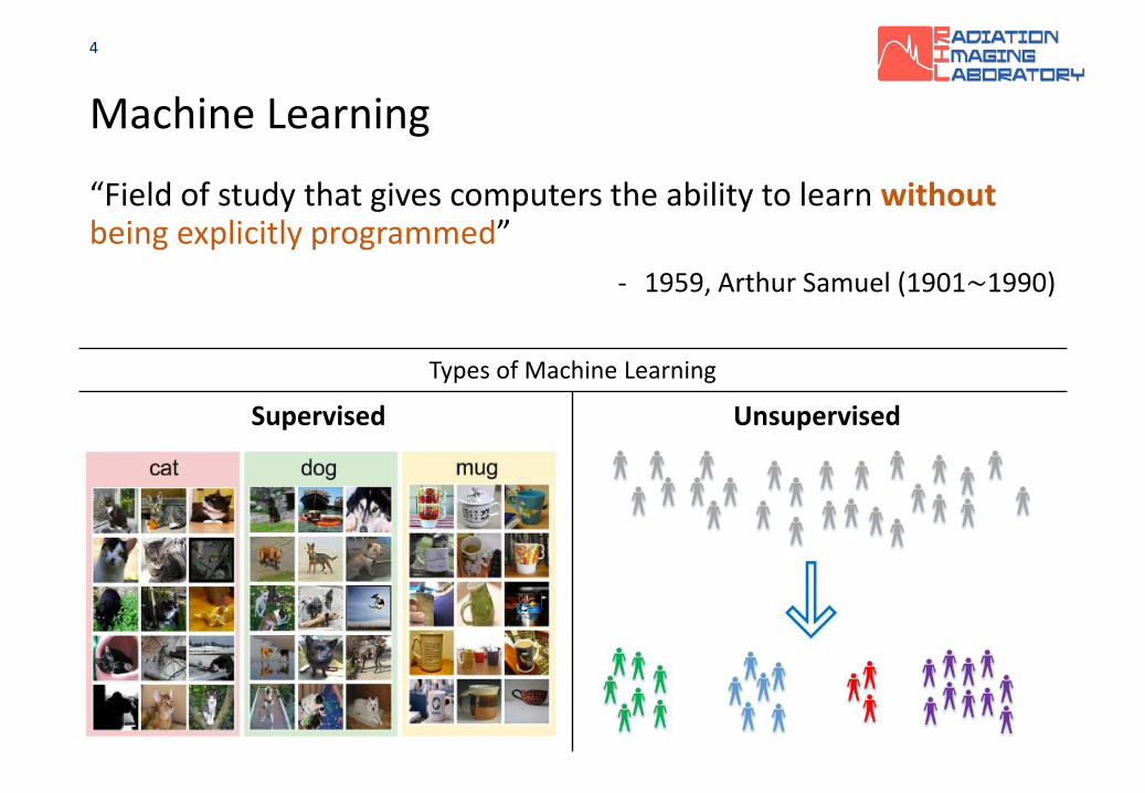
Machine Learning

“Field of study that gives computers the ability to learn withoutbeing explicitly programmed”

- 1959, Arthur Samuel (1901~1990)

Supervised Unsupervised

5

Supervised Learning

1. Regression• Test score based on time spent for study

2. Classification• Pass/Fail based on time spent for study

Hours 2 4 8 12

Score 30 50 80 90

Hours 2 4 8 12

Pass/Fail F F P P

6

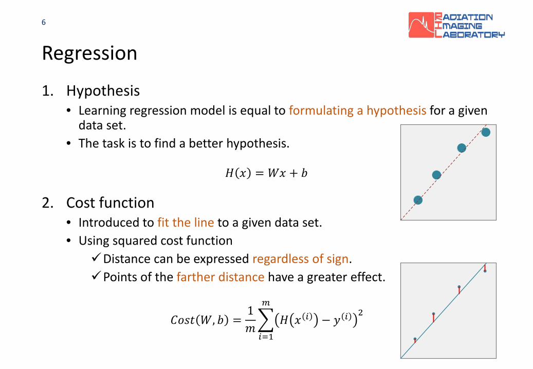
Regression

1. Hypothesis• Learning regression model is equal to formulating a hypothesis for a given

data set.• The task is to find a better hypothesis.

2. Cost function• Introduced to fit the line to a given data set.• Using squared cost function

Distance can be expressed regardless of sign.Points of the farther distance have a greater effect.

𝐻𝐻 𝑥𝑥 = 𝑊𝑊𝑥𝑥 + 𝑏𝑏

𝐶𝐶𝐶𝐶𝐶𝐶𝐶𝐶 𝑊𝑊, 𝑏𝑏 =1𝑚𝑚�

𝑖𝑖=1

𝑚𝑚

𝐻𝐻 𝑥𝑥 𝑖𝑖 − 𝑦𝑦 𝑖𝑖 2

7

Gradient Descent Algorithm• This algorithm is used in many minimization problems.• Formal definition of cost function to minimize cost.

1. Start with initial guesses2. Change some parameters a little bit to reduce cost.3. After modifications, select the gradient which reduces cost the most possible.4. Repeat the above process until you converge to a local minimum.

𝐶𝐶𝐶𝐶𝐶𝐶𝐶𝐶 𝑊𝑊 =12𝑚𝑚�

𝑖𝑖=1

𝑚𝑚

𝑊𝑊𝑥𝑥 𝑖𝑖 − 𝑦𝑦 𝑖𝑖 2

8

Gradient Descent Algorithm• The gradient can be calculated by differentiating the cost function.

𝑊𝑊 ≔ 𝑊𝑊 − 𝜂𝜂𝜕𝜕𝜕𝜕𝑊𝑊

𝐶𝐶𝐶𝐶𝐶𝐶𝐶𝐶(𝑊𝑊)

𝑊𝑊 ≔𝑊𝑊 − 𝜂𝜂𝜕𝜕𝜕𝜕𝑊𝑊

12𝑚𝑚�

𝑖𝑖=1

𝑚𝑚

𝑊𝑊𝑥𝑥 𝑖𝑖 − 𝑦𝑦 𝑖𝑖 2

𝑊𝑊 ≔ 𝑊𝑊 − 𝜂𝜂1𝑚𝑚�

𝑖𝑖=1

𝑚𝑚

𝑊𝑊𝑥𝑥 𝑖𝑖 − 𝑦𝑦 𝑖𝑖 𝑥𝑥 𝑖𝑖

𝑊𝑊 ≔ 𝑊𝑊 − 𝜂𝜂1

2𝑚𝑚�𝑖𝑖=1

𝑚𝑚

2 𝑊𝑊𝑥𝑥 𝑖𝑖 − 𝑦𝑦 𝑖𝑖 𝑥𝑥 𝑖𝑖

In case of the original cost function

𝐶𝐶𝐶𝐶𝐶𝐶𝐶𝐶 𝑊𝑊, 𝑏𝑏 =1𝑚𝑚�𝑖𝑖=1

𝑚𝑚

𝐻𝐻 𝑥𝑥 𝑖𝑖 − 𝑦𝑦 𝑖𝑖 2

𝑊𝑊

𝐶𝐶𝐶𝐶𝐶𝐶𝐶𝐶

𝑏𝑏

9

Expend to Multi-Variables

• Regression using multi-inputs

• Using matrix (Implementation)

• Cost function

𝐻𝐻 𝑥𝑥 = 𝑊𝑊𝑥𝑥 + 𝑏𝑏 𝐻𝐻 𝑥𝑥1, 𝑥𝑥2,⋯ , 𝑥𝑥𝑛𝑛 = 𝑊𝑊1𝑥𝑥1 + 𝑊𝑊2𝑥𝑥2 + ⋯+ 𝑊𝑊𝑛𝑛𝑥𝑥𝑛𝑛 + 𝑏𝑏

𝐶𝐶𝐶𝐶𝐶𝐶𝐶𝐶 𝑊𝑊, 𝑏𝑏 =1𝑚𝑚�

𝑖𝑖=1

𝑚𝑚

𝐻𝐻 𝑥𝑥1𝑖𝑖 , 𝑥𝑥2

𝑖𝑖 ,⋯ , 𝑥𝑥𝑛𝑛𝑖𝑖 − 𝑦𝑦 𝑖𝑖

2

𝑥𝑥1 ⋯ 𝑥𝑥𝑛𝑛 �𝑊𝑊1⋮𝑊𝑊𝑛𝑛

= 𝑥𝑥1𝑊𝑊1 + ⋯+ 𝑥𝑥3𝑊𝑊3𝐻𝐻 𝐗𝐗 = 𝐗𝐗𝐗𝐗

𝐶𝐶𝐶𝐶𝐶𝐶𝐶𝐶 𝐗𝐗 =1𝑚𝑚� 𝐗𝐗𝐗𝐗− 𝑦𝑦 2

10

Classification• The linear hypothesis has several

disadvantages in the classification.

• Other appropriate type of hypothesis

Since derivative is not possible, gradient descent algorithm can not be applied.

11

Logistic Hypothesis• Linear hypothesis

• Logistic hypothesis (Sigmoid)

The sigmoid function is differentiable.

These regression & classification functions are used as the activation function of neural networks.

𝐻𝐻 𝐗𝐗 = 𝐗𝐗𝐗𝐗

𝐻𝐻 𝐗𝐗 =1

1 + 𝑒𝑒−𝐗𝐗𝐗𝐗

𝐻𝐻𝐻 𝐗𝐗 = 𝐻𝐻 𝑿𝑿 1 − 𝐻𝐻 𝑿𝑿

12

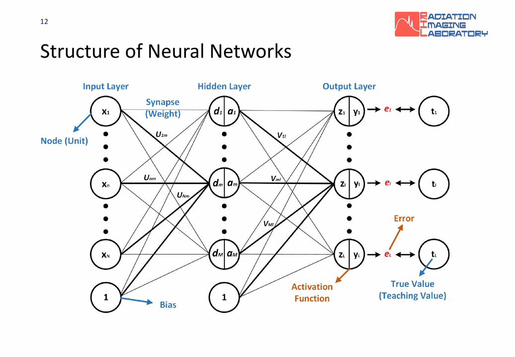
Structure of Neural Networks

13

History of Neural Networks• 1943 McCulloch: logical computation model based on simple neural networks

“A Logical Calculus of The Ideas Immanent in Nervous Activity”

• 1949 Hebb: presentation of learning laws based on synapses.“The Organization of Behavior”

• 1957 Rosenblatt: development of perceptron terminology and algorithm.“The Perceptron, A Perceiving and Recognizing Automaton Project Para”

14

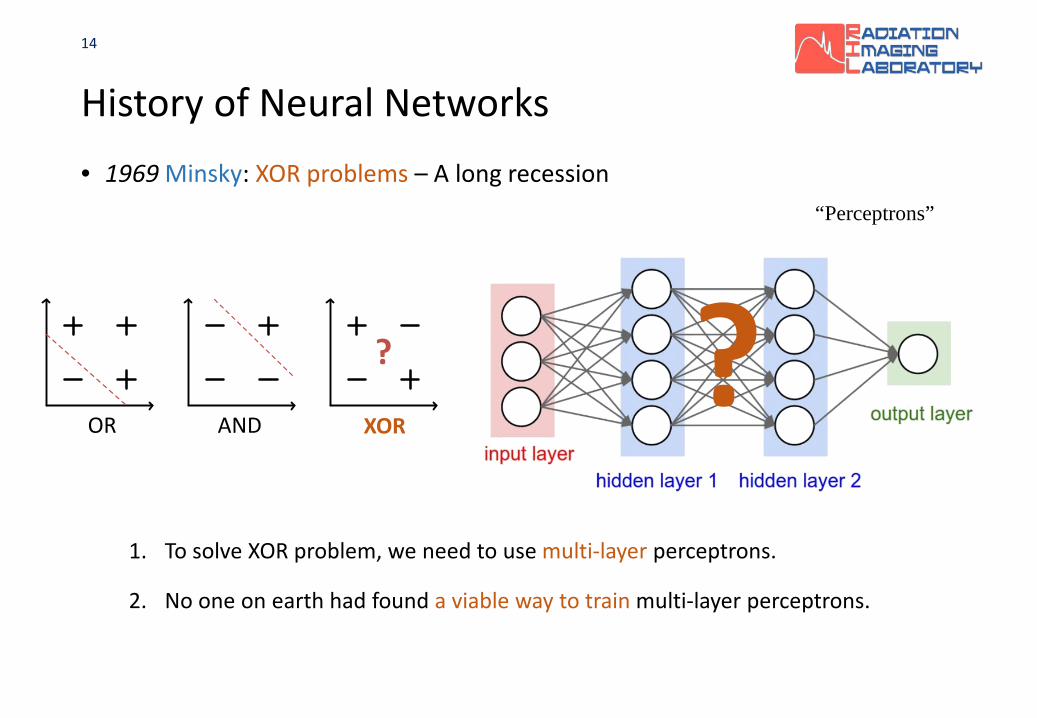
History of Neural Networks• 1969 Minsky: XOR problems – A long recession

“Perceptrons”

1. To solve XOR problem, we need to use multi-layer perceptrons.

2. No one on earth had found a viable way to train multi-layer perceptrons.

?

OR AND XOR?

15

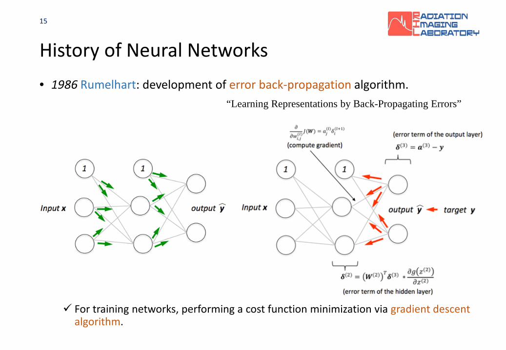
History of Neural Networks• 1986 Rumelhart: development of error back-propagation algorithm.

“Learning Representations by Back-Propagating Errors”

For training networks, performing a cost function minimization via gradient descent algorithm.

16

Application in research

Training Result

Processing

Original RadiographProcessing Result

17

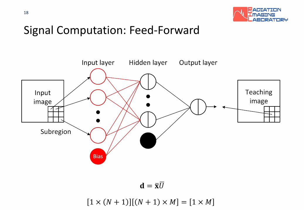
Signal Computation: Feed-Forward

Input signal vector : 𝐱𝐱1 × 𝑁𝑁

18

Signal Computation: Feed-Forward

𝐝𝐝 = �𝐱𝐱�𝑈𝑈

1 × 𝑁𝑁 + 1 𝑁𝑁 + 1 × 𝑀𝑀 = 1 × 𝑀𝑀

19

Signal Computation: Feed-Forward

𝐚𝐚 = 𝑔𝑔 𝐝𝐝 =1

1 − 𝑒𝑒−𝐝𝐝

1 × 𝑀𝑀

20

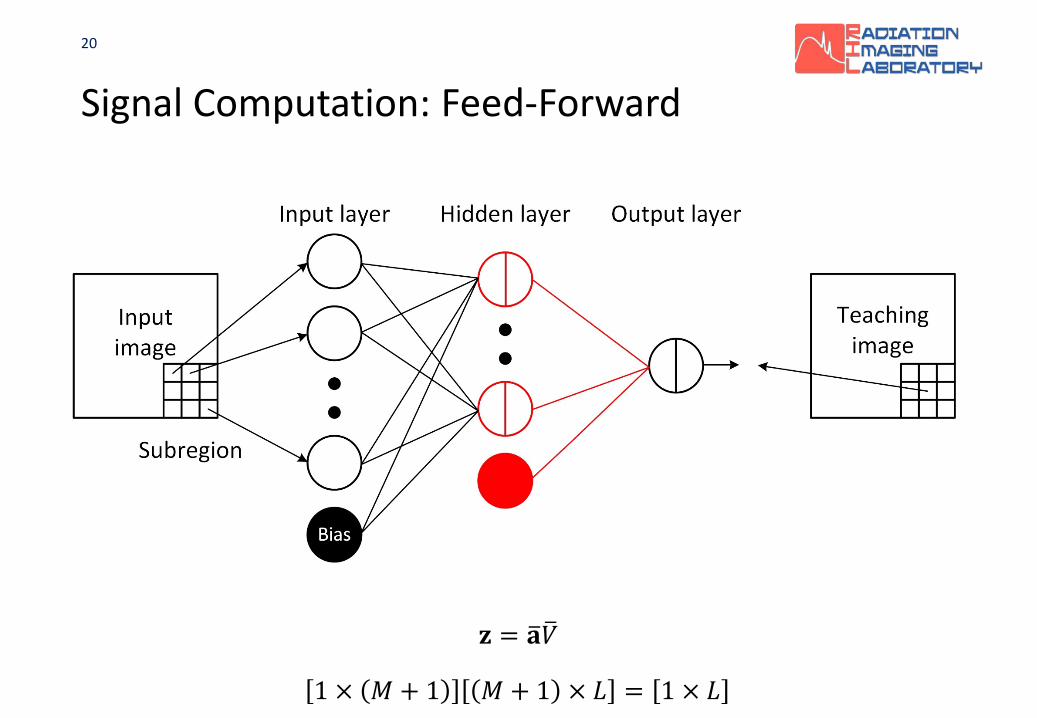
Signal Computation: Feed-Forward

𝐳𝐳 = �𝐚𝐚 �𝑉𝑉

1 × 𝑀𝑀 + 1 𝑀𝑀 + 1 × 𝐿𝐿 = 1 × 𝐿𝐿

21

Signal Computation: Feed-Forward

𝐲𝐲 = ℎ 𝐳𝐳 = 𝛼𝛼𝐳𝐳 + 𝛽𝛽

1 × 𝐿𝐿

22

Signal Computation: Feed-Forward

𝐞𝐞 =12

(𝐲𝐲 − 𝐭𝐭)2

1 × 𝐿𝐿

23

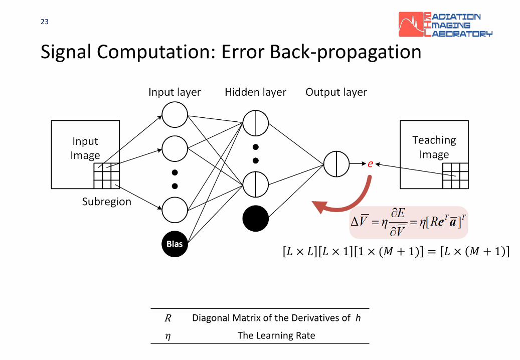
Signal Computation: Error Back-propagation

R Diagonal Matrix of the Derivatives of h

𝜂𝜂 The Learning Rate

𝐿𝐿 × 𝐿𝐿 𝐿𝐿 × 1 1 × (𝑀𝑀 + 1) = 𝐿𝐿 × 𝑀𝑀 + 1

24

Signal Computation: Error Back-propagation

Q Diagonal Matrix of the Derivatives of g

𝜂𝜂 The Learning Rate

𝑀𝑀 × 𝑀𝑀 𝑀𝑀 × 𝐿𝐿 𝐿𝐿 × 𝐿𝐿 𝐿𝐿 × 1 1 × (𝑁𝑁 + 1) = 𝑀𝑀 × 𝑁𝑁 + 1

25

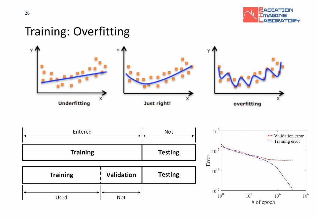
Training: Epoch

26

Training: Overfitting

27

Homework

Training Result

Processing

ReferenceProcessing Result

28

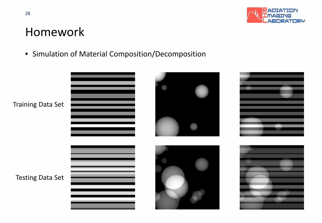
Homework• Simulation of Material Composition/Decomposition

Training Data Set

Testing Data Set

29

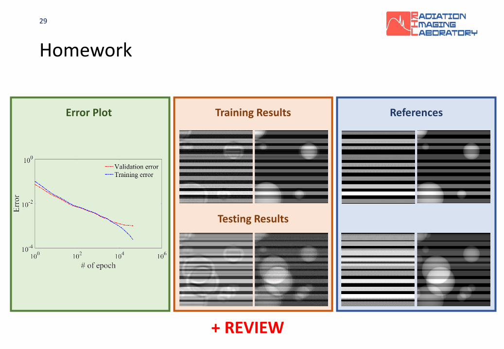
Homework

Training Results ReferencesError Plot

+ REVIEW

Testing Results

30

Into the Deep Learning

• Vanishing Gradient Problem – The deeper? The harder to train!• Rectified Linear Unit (ReLU)

• Prevent overfitting – A burning issue• Data Augmentation• Drop out• Regularization

• Deep Learning Algorithms• Convolutional Neural Networks (CNN): Pattern recognition, Classification• Recurrent Neural Networks (RNN): Sequence data processing, Translation