Machine Learning Lecture 6 · Machine Learning –Lecture 6 Linear Discriminants II 30.10.2019...

Perc

ep

tual

an

d S

en

so

ry A

ug

me

nte

d C

om

pu

tin

gM

achin

e L

earn

ing W

inte

r ‘1

9

Machine Learning – Lecture 6

Linear Discriminants II

30.10.2019

Bastian Leibe

RWTH Aachen

http://www.vision.rwth-aachen.de

[email protected]

Perc

ep

tual

an

d S

en

so

ry A

ug

me

nte

d C

om

pu

tin

gM

achin

e L

earn

ing W

inte

r ‘1

9

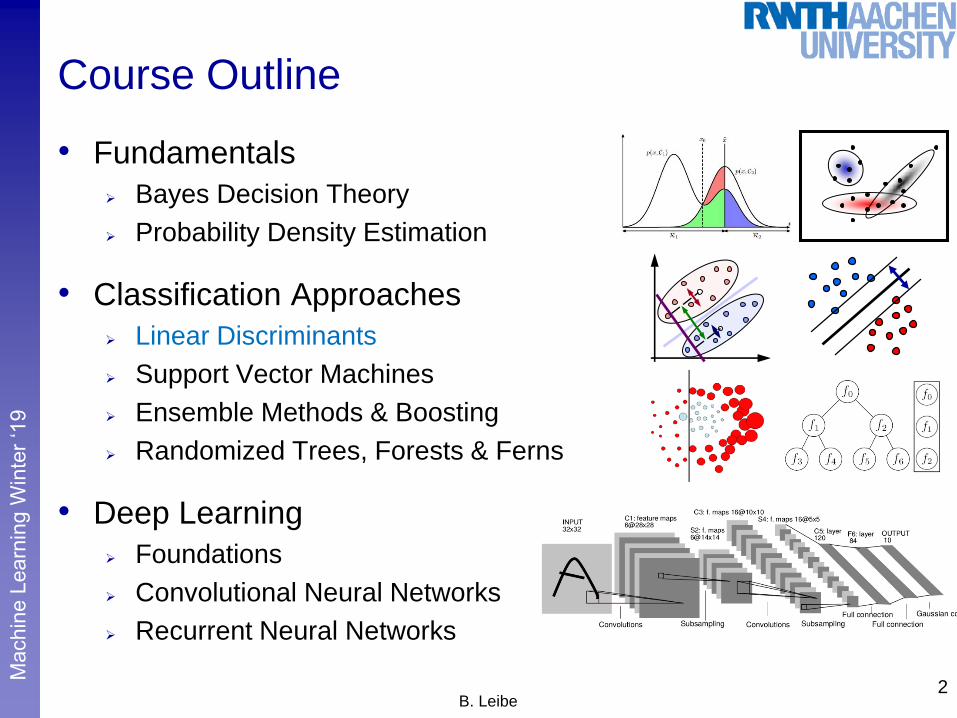
Course Outline

• Fundamentals

Bayes Decision Theory

Probability Density Estimation

• Classification Approaches

Linear Discriminants

Support Vector Machines

Ensemble Methods & Boosting

Randomized Trees, Forests & Ferns

• Deep Learning

Foundations

Convolutional Neural Networks

Recurrent Neural Networks

2B. Leibe

Perc

ep

tual

an

d S

en

so

ry A

ug

me

nte

d C

om

pu

tin

gM

achin

e L

earn

ing W

inte

r ‘1

9

Recap: Linear Discriminant Functions

• Basic idea

Directly encode decision boundary

Minimize misclassification probability directly.

• Linear discriminant functions

w, w0 define a hyperplane in RD.

If a data set can be perfectly classified by a linear discriminant, then

we call it linearly separable.3

B. Leibe

y(x) =wTx+w0

weight vector “bias”

(= threshold)

Slide adapted from Bernt Schiele3

y = 0y > 0

y < 0

Perc

ep

tual

an

d S

en

so

ry A

ug

me

nte

d C

om

pu

tin

gM

achin

e L

earn

ing W

inte

r ‘1

9

Recap: Least-Squares Classification

• Simplest approach

Directly try to minimize the sum-of-squares error

Setting the derivative to zero yields

We then obtain the discriminant function as

Exact, closed-form solution for the discriminant function parameters.

4B. Leibe

ED(fW) =1

2Trn(eXfW¡T)T(eXfW¡T)

o

fW = (eXT eX)¡1 eXTT= eXyT= (eXT eX)¡1 eXTT

y(x) = fWTex = TT³eXy

T́

ex

E(w) =

NX

n=1

(y(xn;w)¡ tn)2

Perc

ep

tual

an

d S

en

so

ry A

ug

me

nte

d C

om

pu

tin

gM

achin

e L

earn

ing W

inte

r ‘1

9

Recap: Problems with Least Squares

• Least-squares is very sensitive to outliers!

The error function penalizes predictions that are “too correct”.5

B. Leibe Image source: C.M. Bishop, 2006

Perc

ep

tual

an

d S

en

so

ry A

ug

me

nte

d C

om

pu

tin

gM

achin

e L

earn

ing W

inte

r ‘1

9

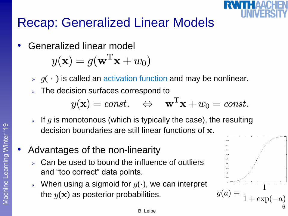
Recap: Generalized Linear Models

• Generalized linear model

g( ¢ ) is called an activation function and may be nonlinear.

The decision surfaces correspond to

If g is monotonous (which is typically the case), the resulting

decision boundaries are still linear functions of x.

• Advantages of the non-linearity

Can be used to bound the influence of outliers

and “too correct” data points.

When using a sigmoid for g(¢), we can interpret

the y(x) as posterior probabilities.

6B. Leibe

y(x) = g(wTx+w0)

y(x) = const: , wTx+w0 = const:

g(a) ´ 1

1 + exp(¡a)

Perc

ep

tual

an

d S

en

so

ry A

ug

me

nte

d C

om

pu

tin

gM

achin

e L

earn

ing W

inte

r ‘1

9

Linear Separability

• Up to now: restrictive assumption

Only consider linear decision boundaries

• Classical counterexample: XOR

8B. LeibeSlide credit: Bernt Schiele

1x

2x

Perc

ep

tual

an

d S

en

so

ry A

ug

me

nte

d C

om

pu

tin

gM

achin

e L

earn

ing W

inte

r ‘1

9

yk(x) =

MX

j=0

wkjÁj(x)

Generalized Linear Discriminants

• Generalization

Transform vector x with M nonlinear basis functions Áj(x):

Purpose of Áj(x): basis functions

Allow non-linear decision boundaries.

By choosing the right Áj, every continuous function can (in principle)

be approximated with arbitrary accuracy.

• Notation

9B. Leibe

yk(x) =

MX

j=1

wkjÁj(x) +wk0

with Á0(x) = 1

Slide credit: Bernt Schiele

Perc

ep

tual

an

d S

en

so

ry A

ug

me

nte

d C

om

pu

tin

gM

achin

e L

earn

ing W

inte

r ‘1

9

Linear Basis Function Models

• Generalized Linear Discriminant Model

where Áj(x) are known as basis functions.

Typically, Á0(x) = 1, so that w0 acts as a bias.

In the simplest case, we use linear basis functions: Ád(x) = xd.

• Let’s take a look at some other possible basis functions...

10B. LeibeSlide adapted from C.M. Bishop, 2006

Perc

ep

tual

an

d S

en

so

ry A

ug

me

nte

d C

om

pu

tin

gM

achin

e L

earn

ing W

inte

r ‘1

9

Linear Basis Function Models (2)

• Polynomial basis functions

• Properties

Global

A small change in x affects all

basis functions.

• Result

If we use polynomial basis functions, the decision boundary will

be a polynomial function of 𝑥.

Nonlinear decision boundaries

However, we still solve a linear problem in 𝜙 𝑥 .

11B. LeibeSlide adapted from C.M. Bishop, 2006 Image source: C.M. Bishop, 2006

Perc

ep

tual

an

d S

en

so

ry A

ug

me

nte

d C

om

pu

tin

gM

achin

e L

earn

ing W

inte

r ‘1

9


• Gaussian basis functions

• Properties

Local

A small change in x affects

only nearby basis functions.

¹j and s control location and

scale (width).


Perc

ep

tual

an

d S

en

so

ry A

ug

me

nte

d C

om

pu

tin

gM

achin

e L

earn

ing W

inte

r ‘1

9


• Sigmoid basis functions

where

• Properties

Local

A small change in x affects

only nearby basis functions.

¹j and s control location and

scale (slope).


Perc

ep

tual

an

d S

en

so

ry A

ug

me

nte

d C

om

pu

tin

gM

achin

e L

earn

ing W

inte

r ‘1

9

Topics of This Lecture

• Gradient Descent

• Logistic Regression Probabilistic discriminative models

Logistic sigmoid (logit function)

Cross-entropy error

Iteratively Reweighted Least Squares

• Softmax Regression Multi-class generalization

Gradient descent solution

• Note on Error Functions Ideal error function

Quadratic error

Cross-entropy error15

B. Leibe

Perc

ep

tual

an

d S

en

so

ry A

ug

me

nte

d C

om

pu

tin

gM

achin

e L

earn

ing W

inte

r ‘1

9

Gradient Descent

• Learning the weights w:

N training data points: X = {x1, …, xN}

K outputs of decision functions: yk(xn;w)

Target vector for each data point: T = {t1, …, tN}

Error function (least-squares error) of linear model

16B. Leibe

E(w) =1

2

NX

n=1

KX

k=1

(yk(xn;w)¡ tkn)2

=1

2

NX

n=1

KX

k=1

0@

MX

j=1

wkjÁj(xn)¡ tkn

1A2


Perc

ep

tual

an

d S

en

so

ry A

ug

me

nte

d C

om

pu

tin

gM

achin

e L

earn

ing W

inte

r ‘1

9

Gradient Descent

• Problem

The error function can in general no longer be minimized in

closed form.

• ldea (Gradient Descent)

Iterative minimization

Start with an initial guess for the parameter values .

Move towards a (local) minimum by following the gradient.

This simple scheme corresponds to a 1st-order Taylor expansion

(There are more complex procedures available).

17B. Leibe

w(¿+1)

kj = w(¿)

kj ¡ ´@E(w)

@wkj

¯̄¯̄w(¿)

´: Learning rate

w(0)

kj

Perc

ep

tual

an

d S

en

so

ry A

ug

me

nte

d C

om

pu

tin

gM

achin

e L

earn

ing W

inte

r ‘1

9

Gradient Descent – Basic Strategies

• “Batch learning”

Compute the gradient based on all training data:

22B. Leibe

w(¿+1)

kj = w(¿)

kj ¡ ´@E(w)

@wkj

¯̄¯̄w(¿)

@E(w)

@wkj


´: Learning rate

Perc

ep

tual

an

d S

en

so

ry A

ug

me

nte

d C

om

pu

tin

gM

achin

e L

earn

ing W

inte

r ‘1

9

Gradient Descent – Basic Strategies

• “Sequential updating”

Compute the gradient based on a single data point at a time:

23B. Leibe

w(¿+1)

kj = w(¿)

kj ¡ ´@En(w)

@wkj

¯̄¯̄w(¿)

´: Learning rate

@En(w)

@wkj

E(w) =

NX

n=1

En(w)


Perc

ep

tual

an

d S

en

so

ry A

ug

me

nte

d C

om

pu

tin

gM

achin

e L

earn

ing W

inte

r ‘1

9

Gradient Descent

• Error function

24B. Leibe

E(w) =

NX

n=1

En(w) =1

2

NX

n=1

KX

k=1

0@

MX

j=1

wkjÁj(xn)¡ tkn

1A2

En(w) =1

2

KX

k=1

0@

MX

j=1

wkjÁj(xn)¡ tkn

1A2

@En(w)

@wkj=

0@

MX

~j=1

wk~jÁ~j(xn)¡ tkn

1AÁj(xn)

= (yk(xn;w)¡ tkn)Áj(xn)


Perc

ep

tual

an

d S

en

so

ry A

ug

me

nte

d C

om

pu

tin

gM

achin

e L

earn

ing W

inte

r ‘1

9

Gradient Descent

• Delta rule (=LMS rule)

where

Simply feed back the input data point, weighted by the

classification error.

25B. Leibe

w(¿+1)

kj = w(¿)

kj ¡ ´ (yk(xn;w)¡ tkn)Áj(xn)

= w(¿)

kj ¡ ´±knÁj(xn)

±kn = yk(xn;w)¡ tkn


Perc

ep

tual

an

d S

en

so

ry A

ug

me

nte

d C

om

pu

tin

gM

achin

e L

earn

ing W

inte

r ‘1

9

Gradient Descent

• Cases with differentiable, non-linear activation function

• Gradient descent

26B. Leibe

yk(x) = g(ak) = g

0@

MX

j=0

wkiÁj(xn)

1A

@En(w)

@wkj=

@g(ak)

@wkj(yk(xn;w)¡ tkn)Áj(xn)

w(¿+1)

kj = w(¿)

kj ¡ ´±knÁj(xn)

±kn =@g(ak)

@wkj(yk(xn;w)¡ tkn)


Perc

ep

tual

an

d S

en

so

ry A

ug

me

nte

d C

om

pu

tin

gM

achin

e L

earn

ing W

inte

r ‘1

9

Summary: Generalized Linear Discriminants

• Properties

General class of decision functions.

Nonlinearity g(¢) and basis functions Áj allow us to address linearly

non-separable problems.

Shown simple sequential learning approach for parameter estimation

using gradient descent.

Better 2nd order gradient descent approaches are available

(e.g. Newton-Raphson), but they are more expensive to compute.

• Limitations / Caveats

Flexibility of model is limited by curse of dimensionality

– g(¢) and Áj often introduce additional parameters.

– Models are either limited to lower-dimensional input space

or need to share parameters.

Linearly separable case often leads to overfitting.

– Several possible parameter choices minimize training error. 27

Perc

ep

tual

an

d S

en

so

ry A

ug

me

nte

d C

om

pu

tin

gM

achin

e L

earn

ing W

inte

r ‘1

9





Cross-entropy error





Quadratic error


B. Leibe

Perc

ep

tual

an

d S

en

so

ry A

ug

me

nte

d C

om

pu

tin

gM

achin

e L

earn

ing W

inte

r ‘1

9

Probabilistic Discriminative Models

• We have seen that we can write

• We can obtain the familiar probabilistic model by setting

• Or we can use generalized linear discriminant models

29B. Leibe

p(C1jx) = ¾(a)

=1

1 + exp(¡a)

a = lnp(xjC1)p(C1)p(xjC2)p(C2)

a =wTx

a =wTÁ(x)

logistic sigmoid

function

or

Perc

ep

tual

an

d S

en

so

ry A

ug

me

nte

d C

om

pu

tin

gM

achin

e L

earn

ing W

inte

r ‘1

9

Probabilistic Discriminative Models

• In the following, we will consider models of the form

with

• This model is called logistic regression.

• Why should we do this? What advantage does such a

model have compared to modeling the probabilities?

• Any ideas?30

B. Leibe

p(C1jÁ) = y(Á) = ¾(wTÁ)

p(C1jÁ) =p(ÁjC1)p(C1)

p(ÁjC1)p(C1) + p(ÁjC2)p(C2)

p(C2jÁ) = 1¡ p(C1jÁ)

Perc

ep

tual

an

d S

en

so

ry A

ug

me

nte

d C

om

pu

tin

gM

achin

e L

earn

ing W

inte

r ‘1

9

Comparison

• Let’s look at the number of parameters…

Assume we have an M-dimensional feature space Á.

And assume we represent p(Á|Ck) and p(Ck) by Gaussians.

How many parameters do we need?

– For the means: 2M

– For the covariances: M(M+1)/2

– Together with the class priors, this gives M(M+5)/2+1 parameters!

How many parameters do we need for logistic regression?

– Just the values of wM parameters.

For large M, logistic regression has clear advantages!

31B. Leibe

p(C1jÁ) = y(Á) = ¾(wTÁ)

Perc

ep

tual

an

d S

en

so

ry A

ug

me

nte

d C

om

pu

tin

gM

achin

e L

earn

ing W

inte

r ‘1

9

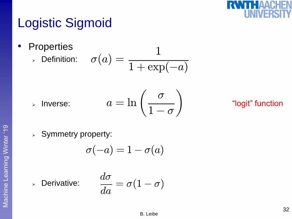
Logistic Sigmoid

• Properties

Definition:

Inverse:

Symmetry property:

Derivative:

32B. Leibe

d¾

da= ¾(1¡ ¾)

¾(a) =1

1 + exp(¡a)

a = ln

µ¾

1¡ ¾

¶

¾(¡a) = 1¡¾(a)

“logit” function

Perc

ep

tual

an

d S

en

so

ry A

ug

me

nte

d C

om

pu

tin

gM

achin

e L

earn

ing W

inte

r ‘1

9

Logistic Regression

• Let’s consider a data set {Án,tn} with n = 1,…,N,

where and , .

• With yn = p(C1|Án), we can write the likelihood as

• Define the error function as the negative log-likelihood

This is the so-called cross-entropy error function.33

Án = Á(xn) tn 2 f0;1g

p(tjw) =

NY

n=1

ytnn f1¡ yng1¡tn

E(w) = ¡ ln p(tjw)

= ¡NX

n=1

ftn ln yn + (1¡ tn) ln(1¡ yn)g

t = (t1; : : : ; tN)T

Perc

ep

tual

an

d S

en

so

ry A

ug

me

nte

d C

om

pu

tin

gM

achin

e L

earn

ing W

inte

r ‘1

9

Gradient of the Error Function

• Error function

• Gradient

34B. Leibe

rE(w) = ¡NX

n=1

(tn

ddw

yn

yn+ (1¡ tn)

ddw

(1¡ yn)

(1¡ yn)

)

= ¡NX

n=1

½tnyn(1¡ yn)

ynÁn ¡ (1¡ tn)

yn(1¡ yn)

(1¡ yn)Án

¾

= ¡NX

n=1

f(tn ¡ tnyn ¡ yn + tnyn)Áng

=

NX

n=1

(yn ¡ tn)Án

E(w) = ¡NX

n=1


yn = ¾(wTÁn)

dyn

dw= yn(1¡ yn)Án

Perc

ep

tual

an

d S

en

so

ry A

ug

me

nte

d C

om

pu

tin

gM

achin

e L

earn

ing W

inte

r ‘1

9

Gradient of the Error Function

• Gradient for logistic regression

• Does this look familiar to you?

• This is the same result as for the Delta (=LMS) rule

• We can use this to derive a sequential estimation algorithm.

However, this will be quite slow…

35B. Leibe

rE(w) =

NX

n=1

(yn ¡ tn)Án

w(¿+1)

kj = w(¿)

kj ¡ ´(yk(xn;w)¡ tkn)Áj(xn)

Perc

ep

tual

an

d S

en

so

ry A

ug

me

nte

d C

om

pu

tin

gM

achin

e L

earn

ing W

inte

r ‘1

9

A More Efficient Iterative Method…

• Second-order Newton-Raphson gradient descent scheme

where is the Hessian matrix, i.e. the matrix

of second derivatives.

• Properties

Local quadratic approximation to the log-likelihood.

Faster convergence.

36B. Leibe

H=rrE(w)

w(¿+1) =w(¿) ¡H¡1rE(w)

Perc

ep

tual

an

d S

en

so

ry A

ug

me

nte

d C

om

pu

tin

gM

achin

e L

earn

ing W

inte

r ‘1

9

Newton-Raphson for Least-Squares Estimation

• Let’s first apply Newton-Raphson to the least-squares

error function:

• Resulting update scheme:

37

E(w) =1

2

NX

n=1

¡wTÁn ¡ tn

¢2

rE(w) =

NX

n=1

¡wTÁn ¡ tn

¢Án = ©T©w¡©T t

H = rrE(w) =

NX

n=1

ÁnÁTn = ©T©

w(¿+1) =w(¿) ¡ (©T©)¡1(©T©w(¿) ¡©Tt)= (©T©)¡1©Tt Closed-form solution!

© =

264ÁT1...

ÁTN

375where

Perc

ep

tual

an

d S

en

so

ry A

ug

me

nte

d C

om

pu

tin

gM

achin

e L

earn

ing W

inte

r ‘1

9

Newton-Raphson for Logistic Regression

• Now, let’s try Newton-Raphson on the cross-entropy error

function:

where R is an NN diagonal matrix with .

The Hessian is no longer constant, but depends on w through the

weighting matrix R.38

B. Leibe

E(w) = ¡NX

n=1


rE(w) =

NX

n=1

(yn ¡ tn)Án = ©T (y¡ t)

H = rrE(w) =

NX

n=1

yn(1¡ yn)ÁnÁTn = ©TR©

Rnn = yn(1¡ yn)

dyn

dw= yn(1¡ yn)Án

Perc

ep

tual

an

d S

en

so

ry A

ug

me

nte

d C

om

pu

tin

gM

achin

e L

earn

ing W

inte

r ‘1

9


• Update equations

• Again very similar form (normal equations)

But now with non-constant weighing matrix R (depends on w).

Need to apply normal equations iteratively.

Iteratively Reweighted Least-Squares (IRLS)39

w(¿+1) =w(¿) ¡ (©TR©)¡1©T (y¡ t)

= (©TR©)¡1n©TR©w(¿) ¡©T (y¡ t)

o

= (©TR©)¡1©TRz

z =©w(¿) ¡R¡1(y¡ t)with

Perc

ep

tual

an

d S

en

so

ry A

ug

me

nte

d C

om

pu

tin

gM

achin

e L

earn

ing W

inte

r ‘1

9

Summary: Logistic Regression

• Properties

Directly represent posterior distribution p(Á|Ck)

Requires fewer parameters than modeling the likelihood + prior.

Very often used in statistics.

It can be shown that the cross-entropy error function is concave

– Optimization leads to unique minimum

– But no closed-form solution exists

– Iterative optimization (IRLS)

Both online and batch optimizations exist

• Caveat

Logistic regression tends to systematically overestimate odds ratios

when the sample size is less than ~500.

40B. Leibe

Perc

ep

tual

an

d S

en

so

ry A

ug

me

nte

d C

om

pu

tin

gM

achin

e L

earn

ing W

inte

r ‘1

9





Cross-entropy error





Quadratic error


B. Leibe

Perc

ep

tual

an

d S

en

so

ry A

ug

me

nte

d C

om

pu

tin

gM

achin

e L

earn

ing W

inte

r ‘1

9

Softmax Regression

• Multi-class generalization of logistic regression

In logistic regression, we assumed binary labels .

Softmax generalizes this to K values in 1-of-K notation.

This uses the softmax function

Note: the resulting distribution is normalized.

42B. Leibe

tn 2 f0;1g

y(x;w) =

26664

P (y = 1jx;w)

P (y = 2jx;w)...

P (y = Kjx;w)

37775 =

1PK

j=1 exp(w>j x)

26664

exp(w>1 x)exp(w>2 x)

...

exp(w>Kx)

37775

Perc

ep

tual

an

d S

en

so

ry A

ug

me

nte

d C

om

pu

tin

gM

achin

e L

earn

ing W

inte

r ‘1

9

Softmax Regression Cost Function

• Logistic regression

Alternative way of writing the cost function

• Softmax regression

Generalization to K classes using indicator functions.

43B. Leibe

E(w) = ¡NX

n=1


= ¡NX

n=1

1X

k=0

fI (tn = k) lnP (yn = kjxn;w)g

E(w) = ¡NX

n=1

KX

k=1

(I (tn = k) ln

exp(w>k x)PK

j=1 exp(w>j x)

)

Perc

ep

tual

an

d S

en

so

ry A

ug

me

nte

d C

om

pu

tin

gM

achin

e L

earn

ing W

inte

r ‘1

9

Optimization

• Again, no closed-form solution is available

Resort again to Gradient Descent

Gradient

• Note

rwk E(w) is itself a vector of partial derivatives for the different

components of wk.

We can now plug this into a standard optimization package.

44B. Leibe

rwkE(w) = ¡NX

n=1

[I (tn = k) lnP (yn = kjxn;w)]

Perc

ep

tual

an

d S

en

so

ry A

ug

me

nte

d C

om

pu

tin

gM

achin

e L

earn

ing W

inte

r ‘1

9





Cross-entropy error





Quadratic error


B. Leibe

Perc

ep

tual

an

d S

en

so

ry A

ug

me

nte

d C

om

pu

tin

gM

achin

e L

earn

ing W

inte

r ‘1

9

Note on Error Functions

• Ideal misclassification error function (black)

This is what we want to approximate (error = #misclassifications)

Unfortunately, it is not differentiable.

The gradient is zero for misclassified points.

We cannot minimize it by gradient descent. 47Image source: Bishop, 2006

Ideal misclassification error

Not differentiable!

zn = tny(xn)

Perc

ep

tual

an

d S

en

so

ry A

ug

me

nte

d C

om

pu

tin

gM

achin

e L

earn

ing W

inte

r ‘1

9

Note on Error Functions

• Squared error used in Least-Squares Classification

Very popular, leads to closed-form solutions.

However, sensitive to outliers due to squared penalty.

Penalizes “too correct” data points

Generally does not lead to good classifiers. 48Image source: Bishop, 2006


Squared error

Penalizes “too correct”

data points!

Sensitive to outliers!

zn = tny(xn)

Perc

ep

tual

an

d S

en

so

ry A

ug

me

nte

d C

om

pu

tin

gM

achin

e L

earn

ing W

inte

r ‘1

9

Comparing Error Functions (Loss Functions)

• Cross-Entropy Error

Minimizer of this error is given by posterior class probabilities.

Concave error function, unique minimum exists.

Robust to outliers, error increases only roughly linearly

But no closed-form solution, requires iterative estimation. 49Image source: Bishop, 2006


Cross-entropy error

Squared error

Robust to outliers!

zn = tny(xn)

Perc

ep

tual

an

d S

en

so

ry A

ug

me

nte

d C

om

pu

tin

gM

achin

e L

earn

ing W

inte

r ‘1

9

Overview: Error Functions

• Ideal Misclassification Error

This is what we would like to optimize.

But cannot compute gradients here.

• Quadratic Error

Easy to optimize, closed-form solutions exist.

But not robust to outliers.

• Cross-Entropy Error

Minimizer of this error is given by posterior class probabilities.

Concave error function, unique minimum exists.

But no closed-form solution, requires iterative estimation.

Looking at the error function this way gives us an analysis

tool to compare the properties of classification approaches.50

B. Leibe

Perc

ep

tual

an

d S

en

so

ry A

ug

me

nte

d C

om

pu

tin

gM

achin

e L

earn

ing W

inte

r ‘1

9

Let’s Put This To Practice…

• Squared error on sigmoid/tanh output function

Avoids penalizing “too correct” data points.

But: zero gradient for confidently incorrect classifications!

Do not use L2 loss with sigmoid outputs (instead: cross-entropy)!

51Image source: Bishop, 2006


Squared error

No penalty for

“too correct”

data points!

Zero gradient!

zn = tny(xn)

Squared error on tanh

Perc

ep

tual

an

d S

en

so

ry A

ug

me

nte

d C

om

pu

tin

gM

achin

e L

earn

ing W

inte

r ‘1

9

References and Further Reading

• More information on Linear Discriminant Functions can be

found in Chapter 4 of Bishop’s book (in particular Chapter

4.1 - 4.3).

52B. Leibe

Christopher M. Bishop

Pattern Recognition and Machine Learning

Springer, 2006

Machine Learning Lecture 6 · Machine Learning –Lecture 6 Linear Discriminants II 30.10.2019...

Documents

Transcript of Machine Learning Lecture 6 · Machine Learning –Lecture 6 Linear Discriminants II 30.10.2019...