Machine Learning Involvement in Reservoir Simulation by ...
63
University of Calgary PRISM: University of Calgary's Digital Repository Graduate Studies The Vault: Electronic Theses and Dissertations 2017 Machine Learning Involvement in Reservoir Simulation by Optimizing Algorithms in SAGD and SA-SAGD Processes Zhang, Yu Zhang, Y. (2017). Machine Learning Involvement in Reservoir Simulation by Optimizing Algorithms in SAGD and SA-SAGD Processes (Unpublished master's thesis). University of Calgary, Calgary, AB. doi:10.11575/PRISM/26806 http://hdl.handle.net/11023/3757 master thesis University of Calgary graduate students retain copyright ownership and moral rights for their thesis. You may use this material in any way that is permitted by the Copyright Act or through licensing that has been assigned to the document. For uses that are not allowable under copyright legislation or licensing, you are required to seek permission. Downloaded from PRISM: https://prism.ucalgary.ca
Transcript of Machine Learning Involvement in Reservoir Simulation by ...

University of Calgary
PRISM: University of Calgary's Digital Repository
Graduate Studies The Vault: Electronic Theses and Dissertations
2017
Machine Learning Involvement in Reservoir
Simulation by Optimizing Algorithms in SAGD and
SA-SAGD Processes
Zhang, Yu
Zhang, Y. (2017). Machine Learning Involvement in Reservoir Simulation by Optimizing
Algorithms in SAGD and SA-SAGD Processes (Unpublished master's thesis). University of Calgary,
Calgary, AB. doi:10.11575/PRISM/26806
http://hdl.handle.net/11023/3757
master thesis
University of Calgary graduate students retain copyright ownership and moral rights for their
thesis. You may use this material in any way that is permitted by the Copyright Act or through
licensing that has been assigned to the document. For uses that are not allowable under
copyright legislation or licensing, you are required to seek permission.
Downloaded from PRISM: https://prism.ucalgary.ca

UNIVERSITY OF CALGARY
Machine Learning Involvement in Reservoir Simulation by Optimizing Algorithms in SAGD
and SA-SAGD Processes
by
Yu Zhang
A THESIS
SUBMITTED TO THE FACULTY OF GRADUATE STUDIES
IN PARTIAL FULFILMENT OF THE REQUIREMENTS FOR THE
DEGREE OF MASTER OF ENGINEERING
GRADUATE PROGRAM IN CHEMICAL AND PETROLEUM ENGINEERING
CALGARY, ALBERTA
APRIL, 2017
© Yu Zhang 2017

ii
ABSTRACT
Machine learning, as a subset of Artificial Intelligence, has invaded many industries in recent
years, thanks to the advancement of the computing power. Over the past decade, the use of
machine learning, predictive analytics, and other artificial intelligence-based technologies in the
oil and gas industry has grown immensely.
Global optimization techniques are useful tools for process optimization and design in various
petroleum-engineering disciplines. In this research, the genetic algorithm, one of the global
optimization branches, acts as the optimizer for the Steam-Assisted Gravity Drainage (SAGD)
process and for the Solvent-Assisted Steam-Assisted Gravity Drainage (SA-SAGD) process.
Both binary and continuous encoding techniques that are embedded in a Computer Modeling
Group (CMG) simulator STARS perform the primary role to optimize the simulation results. In
the end, the comparison with a gradient-based optimization algorithm is studied. The genetic
algorithm optimizer coupled with a reservoir simulator is employed to optimize the steam
injection rates over the life of a steam-assisted gravity drainage process in a particular reservoir.
A concise comparison between the genetic algorithm and a back propagation method discloses
the advantages of the genetic algorithm.
In the end, the simulation results for various scenarios illustrate the impacts brought by the
optimization tool that is coded in programming language Python. The conclusion may be
effective in the specific reservoir condition only, though it indicates a worth-trying approach to
optimize the SAGD and SA-SAGD operations for various reservoirs.

iii
ACKNOWLEDGEMENTS
First and foremost, I would like to express my sincere gratitude and deepest appreciation to my
supervisor, Dr. Zhangxing (John) Chen, for the guidance on the research direction, the advice on
developing the thesis, and valuable critics on the conclusion during the journey of the research.
My sincere thank also gives to Mr. Hui Liu, Ms. Qiong Wang, Mr. Bo Yang and Mr. Mohsen
Keshavarz from Dr. Chen's research group for their help on laboratory tests, thesis structuring
and valuable insights. In addition, special thanks go to the Reservoir Simulation Group as well
led by Dr. Chen; the group’s atmosphere of striving for excellence has inspired me deeply. I am
so proud of being a member of such a research-focused team.
I would like to say thanks to my Mom and Dad, who are all in the early eighties, and they are so
excited to hear that one of their sons has a privilege to challenge for a Master Degree in Canada.
To my elder daughter Jiya, to my younger daughter Jade and to my wife Hua, since it is such a
great thing to conduct the research while the daughters are witnessing how an academic life
looks like.

iv
TABLE OF CONTENTS
CHAPTER 1 Introduction on Machine Learning……………………………………………1
1.1 Introduction on Machine Learning Application in the Oil and Gas Industry....................1
1.2 Introduction on Reservoir Simulators................................................................................5
CHAPTER 2 Introduction on SAGD and SA-SAGD .............................................................8
2.1 Introduction on Steam-Assisted Gravity Drainage (SAGD)..............................................8
2.2 Introduction on Solvent-Assisted Steam-Assisted Gravity Drainage SA-SAGD...............9
2.3 Comparison between SAGD and SA-SAGD …..………………...................................... 10
CHAPTER 3 Optimization Process Design …........................................................................15
3.1 Introduction of STARS......................................................................................................15
3.2 Literature Review on Algorithm Involvement...................................................................15
3.3 Diagram for Optimization in SAGD and SA-SAGD Processes …...................................18
3.4 Selection of Optimization Techniques for SAGD and SA-SAGD Processes ……...........21
CHAPTER 4 Execution of Genetic Algorithm Optimizer in CMG STARS Environment.....25
4.1 Methodology and Model Details .................. ....................................................................25
4.2 The Pre-processing.............................................................................................................27
4.3 Implementation of Optimization Process …......................................................................31
4.4 The Post-processing ..........................................................................................................33
4.5 Comparison with a Gradient-based Method ……………………………………………..34
4.5.1 The Backpropagation Method ........................................................................................34
4.5.2 Comparison.....................................................................................................................34
4.6 Simulation Results Enhanced by the Optimization Tool………………………………...35
CHAPTER 5 Conclusions and Recommendations on Future Work……………….………...42
5.1 Conclusions …………………………………………………………………………..…..42
5.2 Recommendations………………………………………………………………………...46
REFERENCES………………………………………………………………………………..49

v
LIST OF TABLES
Table 4.1 The single-point crossover method in the genetic algorithm....................................30
Table 4.2 Comparison between genetic algorithm and backpropagation ……........................35
Table 4.3 Parameters for NPV calculations in the SAGD process...........................................39
Table 4.4 Parameters for NPV calculations in the SA-SAGD process…….............................40
Table 4.5 Summary of the NPV calculations ………………………………...............................40

vi
LIST OF FIGURES
Figure 1-1 Diagram of Machine Learning Process …………………..………………………...4
Figure 2.1 SAGD Process Schematic Presentation .....................................................................9
Figure 2.2 SAGD Chamber Cross-sectional Representation……………………..….................9
Figure 3.1 Mathematic Model in Optimization Problem............................................................19
Figure 3.2 Diagram of Optimization Process…………….….....................................................20
Figure 3.3 Schematic of Nonlinear Techniques ..…..…………….………….............................22
Figure 3.4 Optimization Process Presented in Genetic Algorithm Processing............................24
Figure 4.1 Description of the Reservoir ……………………………………………..................26
Figure 4.2 The Flowchart of the Genetic Algorithm…................................................................32
Figure 4.3 Accumulative Steam-Oil Ratio Chart…….................................................................36
Figure 4.4 Accumulative Water SC Chart...................................................................................36
Figure 4.5 Base Case…………………………………………………………………................37
Figure 4.6 Scenario 1.................................................................................................................. 37
Figure 4.7 Scenario 2……...........................................................................................................38
Figure 4.8 Scenario 3...................................................................................................................38
Figure 4.9 Scenario 4…………………………………………………………………................39

1. Introduction on Machine Learning
1.1 Introduction on Machine Learning Application in the Oil and Gas Industry
Machine learning is to use example data to solve a given task without providing explicitly a
program to computers. It has been widely employed in a range of computing tasks for several
decades, including the tasks in the oil and gas industry. Over the past decade, the use of
machine learning, predictive analytics, and other artificial intelligence-based technologies in
the oil and gas industry has grown immensely. Particularly, in the past two years, the
plummeting oil price has driven oil producers and oil service companies to strive for higher
efficiency, lower operational costs, and less unscheduled downtime. An IT technology
including data mining and the machine learning technique have been adopted in an
unprecedented speed in the oil and gas industry thanks to the vast amount of history data.
Prediction of reservoir production contains a series of complex tasks such as data fusion (i.e.,
integration of data from various sources), data mining (i.e., information retrieval after
analyzing data), data selection for training, verification of a design, and integration into an
existing system.
In the domain of machine learning, there are various types to define what the popular algorithms
are. For the introduction purpose, the types of algorithms contributed by Ray (2015) have been
used to outline three categories of mainstream algorithms: Supervised Learning, Unsupervised
Learning, and Reinforcement Learning. The first category consists of a target / outcome variable
(or dependent variable) which is to be predicted from a given set of predictors (independent
variables). Using this set of variables, we generate a function that maps inputs to desired outputs.
The training process continues until the model achieves a desired level of accuracy on the training
2
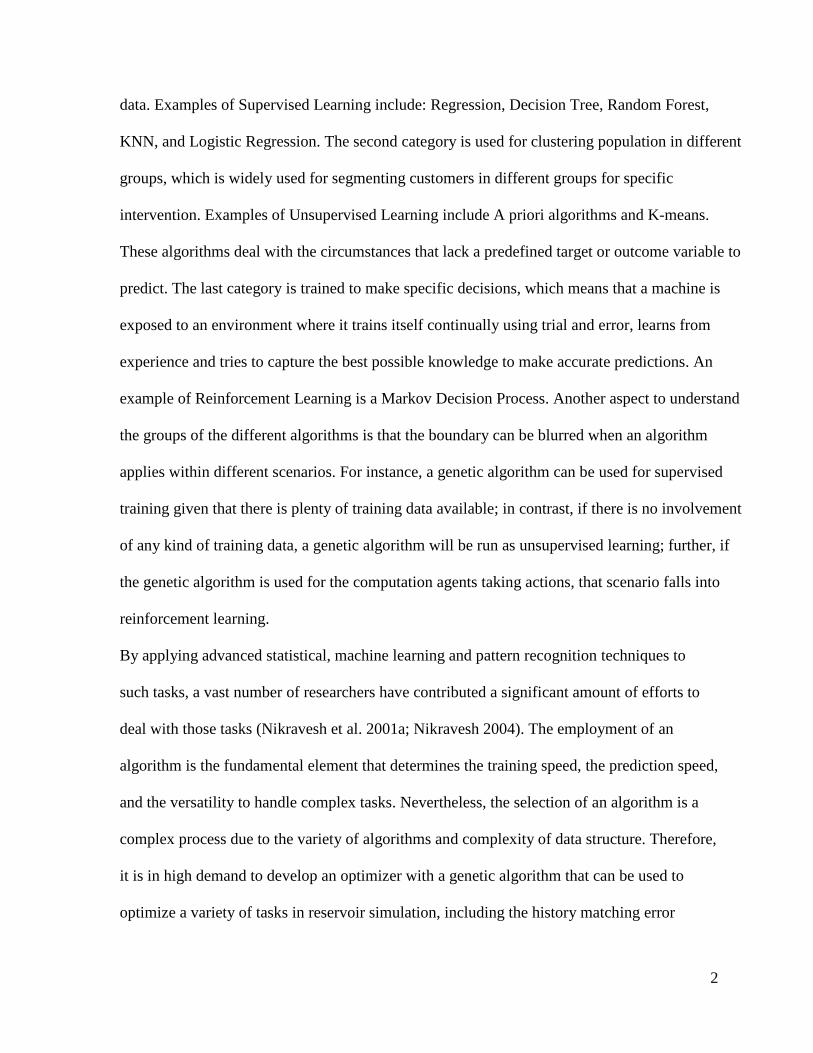
data. Examples of Supervised Learning include: Regression, Decision Tree, Random Forest,
KNN, and Logistic Regression. The second category is used for clustering population in different
groups, which is widely used for segmenting customers in different groups for specific
intervention. Examples of Unsupervised Learning include A priori algorithms and K-means.
These algorithms deal with the circumstances that lack a predefined target or outcome variable to
predict. The last category is trained to make specific decisions, which means that a machine is
exposed to an environment where it trains itself continually using trial and error, learns from
experience and tries to capture the best possible knowledge to make accurate predictions. An
example of Reinforcement Learning is a Markov Decision Process. Another aspect to understand
the groups of the different algorithms is that the boundary can be blurred when an algorithm
applies within different scenarios. For instance, a genetic algorithm can be used for supervised
training given that there is plenty of training data available; in contrast, if there is no involvement
of any kind of training data, a genetic algorithm will be run as unsupervised learning; further, if
the genetic algorithm is used for the computation agents taking actions, that scenario falls into
reinforcement learning.
By applying advanced statistical, machine learning and pattern recognition techniques to
such tasks, a vast number of researchers have contributed a significant amount of efforts to
deal with those tasks (Nikravesh et al. 2001a; Nikravesh 2004). The employment of an
algorithm is the fundamental element that determines the training speed, the prediction speed,
and the versatility to handle complex tasks. Nevertheless, the selection of an algorithm is a
complex process due to the variety of algorithms and complexity of data structure. Therefore,
it is in high demand to develop an optimizer with a genetic algorithm that can be used to
optimize a variety of tasks in reservoir simulation, including the history matching error

3
minimization, an optimal field development plan, production optimization and process
optimization.
In this thesis, two algorithms are listed as examples to contrast different algorithms:
Penalized Linear Regression and Ensemble Methods. Penalized linear regression is a
derivative of ordinary least squares (OLS) regression that was originally developed by Gauss
and Legendre. Penalized linear regression methods were designed to overcome some basic
limitations of OLS regression. The primary limitation of OLS is the biased impact brought by
outliers that are far away from the majority of independent variables. Penalized linear
regression provides a way to systematically reduce degrees of freedom to match the amount
of data available and the complexity of the underlying phenomena. Linear models tend to
train rapidly and often give equivalent performance to nonlinear ensemble methods,
especially when the data availability is an issue. In contrast, Ensemble Methods are building
a group of different predictive models, combining all the outputs, and then averaging the
outputs or taking the majority answer (voting) to generate the best possible predictions.
Ensemble methods have followed a development path parallel to penalized linear regression.
Unlike penalized linear regression evolved from overcoming the limitations of OLS,
Ensemble Methods evolved to overcome the limitations of binary decision trees. Typical
examples include K nearest neighbors (KNNs), artificial neural nets (ANNs), and support
vector machines (SVMs).
Apart from carrying a much faster training time advantage, Penalized Linear Methods predict
much faster than ensemble methods. For highly time‐sensitive predictions such as high‐
speed trading or Internet ad insertions, computation duration determines the level of
profitability, whereas the Ensemble Methods are associated a unique advantage to handle the

4
complex tasks. Therefore, reservoir simulators normally adopt one or more ensemble
methods thanks to the complexity of the subsurface properties. The typical diagram of the
machine learning process is as follows:
Furthermore, the involvement of Fuzzy Logic has been attempted by Rogers et al. (1992),
Lim (2005), Aminian et al. (2005) and Kaydani et al. (2012) to simulate the impacts
associated with versatileness of rocks.
Data preparation and feature engineering are estimated to take 80 to 90 percent of the time
required to develop a machine learning model. The nonlinearity associated with complex
data involved in reservoir simulation, such as Bottom Hole Pressure, Pre-Heating Time, and
Well Locations, poses peculiar challenges to the simulation process. Hampson et al. (2001),
Wong (2002), Guo et al. (2010) and Ahmadi et al. (2013) have tried innovative approaches
for nonlinear tasks with neural networks, Neuro-fuzzy Systems, expert systems, and multiple
regression, respectively.
Step 1
Quantitative
Task
Explanation
Step 2
Mathematically
Task
Explanation
Step 3
Model
Training
Execution
Step 5
Model
Deployment
Step 4
Validation
Testing
Integration
Task Reframe
Algorithm Redesign
Figure 1-1 Diagram of Machine Learning Process

5
1.2 Introduction on Reservoir Simulators
Unconventional hydrocarbon resources represent a growing force in the entire energy reserve
realm, including Tight Gas Production, Tight Oil Production, Shale Gas, and Coalbed
Methane. A reservoir simulator plays an essential role to rationalize the millions dollars spent
by predicting the behavior of hydrocarbon components beneath thousands of feet of
overburden. By combing the theories from physics, mathematics, reservoir engineering and
computer programming, the reservoir simulation explores the best possible solution to
uncover the underground resources. Accordingly, many novel subsurface processes
associated with tremendous commercial potential together with lofty technological risks are
playing an important part in terms of the reserve exploration. Normally, in order to unlock
the unconventional reserves, the timeline from feasibility studies, lab testing and pilot
projects till commercialization are in the order of tens of years. The typical timeline of
Enhanced Oil Recovery (EOR) projects in the oil and gas industry requires about 10 years.
Therefore, the simulators that can mimic the subsurface operations are in high demand, by
predicting the inputs required and outputs generated in a timely and accurate fashion. The
effective simulation operations, or the capable simulators, perform the role of maximizing the
production of hydrocarbon resources and rationalizing the spending of operations.
Nevertheless, the constant challenges for the existing simulators are arisen from two aspects:
the ever-growing complexity of a task and rapidly changing computer architecture. The
complexity is that the formation is heterogeneous, shale is ultra-tight, and the physics
including rock properties and flow mechanisms is uncertain. On the other hand, thanks to the
capability of prediction and generalization enabled by approximating complex and
nonlinearity relationship between input and output variables, Artificial Neural Network
6
(ANN) has been widely used to model single or multiple target properties from predictor
variables in various industries. For instance, Kaastra et al. (1996) introduced the application
of ANN in financial time series; España-Boquera et al. (2007) studied the application of
ANN in text recognition application; Ostlin et al. (2012) studied the application of ANN in
telecommunications; Ali et al. (2012) studied the application of ANN in the ocean
engineering industry; Sharma et al. (2013) introduced the application of ANN in climate
research; and ANN applications in reservoir characterization have been researched by
Nikravesh et al. (2001b), Lim (2005), Eren et al. (1997), Wong et al. (1995), Nikravesh et al.
(2003) and Chaki et al. (2014). Furthermore, a hybrid system contains a modular network
and conventional ANN has been studied by various researchers with the conclusion that the
hybrid system, so-called modular artificial neural networks (MANN) prevails solely the
ANN architecture to solve complex nonlinear problems (Smaoui et al. 1997, Auda et al.
1999, Jiang et al. 2003, Al-Bulushi et al. 2009, Asadi et al. 2013, Al-Dousari et al. 2013).
With the tailor-made algorithm for each specific module, the advantage of a hybrid
architecture comes with the design of separating a complicated task into a series of sub-tasks;
then the sub-tasks can be handled by various modules that are specially designed for each
task; in the end of the process, the sub-results will be merged to accomplish the ultimate
result for the original complex task. This approach is particularly suitable for the reservoir
simulation software thanks to the inherent heterogeneous nature of a subsurface system
(Jiang et al. 2003, Mendoza et al. 2009, Ding et al. 2014, Sánchez et al. 2014). History
matching, by identifying a set of parameters that minimize the difference between the model
performance and the historical performance of a reservoir, is an inverse process. The
mathematical theory presents as follows:

7
The law of mass conservation (Chen 2007):
ϕ𝜕𝑡𝜌𝛼𝑠𝛼 = -∇. (𝜌𝛼 𝑣𝛼 ) + 𝑄𝛼
The Darcy Law:
𝑣𝛼 =𝐾 𝑘𝑟𝛼 (𝑠𝛼 )
𝜇𝛼 ∇𝑝𝛼 ,
where
ϕ: Porosity of the porous media
𝜌𝛼: Density of the phase α
𝑠𝛼: Saturation of the phase α
𝑣𝛼 : Volumetric velocity of phase α
𝑄𝛼 : Flow rate in wells of phase α
K: Permeability of porous media
𝑘𝑟𝛼: The relative permeability of phase α
𝜇𝛼: The viscosity of phase α
𝑝𝛼: The pressure of phase α
In this thesis, the reservoir is three-dimensional with three phases (water, oil and gas), and
the reservoir is incompressible and immiscible with gravity-free environment. The capillary
pressure is null, which means all the 𝑝𝛼s have the same value.

8
2. Introduction on SAGD and SA-SAGD
2.1 Introduction on Steam-Assisted Gravity Drainage (SAGD)
Western Canada’s remaining bitumen reserves in the oil sands have been estimated at more
than 166 billion barrels (Government of Alberta 2014). The open pit mining technology has
been adopted to unlock the shallow bitumen resources that reside 70 meters or less from the
surface; the rest that represents the vast majority of the total bitumen resource has to be
extracted with various in-situ technologies. In the last decade, Steam Assisted Gravity
Drainage (SAGD) has been deployed as the technology of choice to produce these
recoverable reserves. Steam Assisted Gravity Drainage (SAGD) is a thermal in situ recovery
method that involves drilling two horizontal wells that are separated by a distance (typically
3 – 7 m) (Butler 1996). High pressure steam is continuously injected through the upper
wellbore, where it rises, forms a steam chamber, and then fills the void space left by the
heated oil that has a lower viscosity and flows via gravity driven drainage into the lower
wellbore. Condensed water and crude oil are recovered at the surface by pumps. The
indicators of the performance of the SAGD process are:
The amount of steam involved
The heavy oil production rate
The ultimate heavy oil recovery rate
Due to the nature of the SAGD technology that requires significant amount of steam injected
into an underground reservoir, the process associated with heavy environmental footprint has
been investigated for carbon emission. One of the possible improvements is to adopt solvent
injection, either solvent injected with steam or solvent injected solely. In the process of
SAGD, water consumption that aims to generate high quality steam poses the greatest

9
challenge on both operational costs and environmental impact, as the process requires natural
gas burned to vaporize the water, which generates a vast amount of greenhouse gas emissions
(Giacchetta et al. 2015). Meanwhile, the treatment of the processing water pertains to
additional operation expense.
Figure 2.1 SAGD Process Schematic Representation
Figure 2.2 SAGD Chamber Cross-sectional Representation
Source: Japan Canada Oil Sands Limited

10
Apart from environmental concerns, the SAGD process is ineffective and insecure if the pay
zones are thin due to the excessive heat loss and cap rock integrity issue. Similarly, if the
carbonate reservoirs have a low permeability or if the overburdens of the reservoirs are
aquifers or gas, the SAGD process hardly performs as a viable extraction technology.
Therefore, there is a need on developing innovative extraction technologies to accommodate
the environmental challenges and to adapt the special geology formations.
2.2 Introduction on Solvent-Assisted Steam-Assisted Gravity Drainage SA-SAGD
As a non-thermal process, in a similar fashion to SAGD, the Solvent-Assisted Steam-
Assisted Gravity Drainage (SA-SAGD) process employs a pair of wells, through which a
gaseous solvent is injected into the upper horizontal injection well that locates in the
reservoir. Then the solvent-diluted heavy oil is drained downward under the influence of
gravity and collected in the lower horizontal production well (Butler et al. 1991, Das 1998).
In the SA-SAGD process, solvent vapor dissolves at the interface between solvent and heavy
oil and diffuses through the oil. Just like in the SAGD process, the less viscous heavy oil
flows along the edge of a vapor chamber to the production well. In the early stage, Butler and
Mokrys (1989) initially analytically investigated the SA-SAGD process in a vertical Hele–
Shaw cell by selecting toluene as an extracting solvent to dissolve two different bitumen
samples in the laboratory. An analytical model was created to simulate the steady bitumen
production rate during the solvent chamber-spreading phase in the Hele–Shaw cell under the
SA-SAGD process (Butler et al. 1989). Afterwards, this Butler–Mokrys analytical model has
been adjusted by introducing the cementation factor (Das et al. 2008). Nevertheless, the
measured heavy oil production rates in different sand-packs are about various parameters to
one order higher than the predictions from the Butler–Mokrys model (Dunn et al., 1989, Das

11
and Butler, 1996 and Lim et al., 1996). Research conducted by Boustani and Maini (2001)
has concluded that the condition of achieving the agreement between computerized
predictions and lab experimental results is the involvement of the modified Butler–Mokrys
model that depicts the convective dispersion effect on the solvent dissolution into the heavy
oil sample through a porous media. Moreover, due to the analytical models’ dependence on
experiment parameters, there is an intensive discussion on the accuracy of determination on a
dispersion coefficient in recent years (Upreti et al. 2007).
2.3 Comparison between SAGD and SA-SAGD
Compared with SAGD extraction, co-injection containing steam together with solvent results
in a high oil production rate and a lower steam-oil ratio, which has been analyzed in various
papers (Yazdani et al. 2011, Li et al. 2011, Ivory et al. 2008, Govind et al. 2008, Gupata et al.
2012, Leaute et al. 2005, Nasr et al. 2006, Leaute 2002). Due to the complexity of the
multiphase behavior associated with solvent, steam, water, and asphaltene, those literature
reports were discussed based on a simplified scenario within specific reservoir conditions. In
addition, those studies were primarily focused on the selection of the solvent and its
concentration; for instance, Yazdani et al. (2011) concluded that C6 and C7 were the
preferred choices, whereas Govind et al. (2008) identified that C4 generated a higher oil
production rate with 4000KPa as operating pressure. It is possible to achieve a higher oil
production rate while maintaining a lower solvent retention rate in-situ by controlling the
concentration of a given co-injection solvent (Keshavarz et al. 2014). There is need to further
investigate the impact brought by temperature and pressure on the recovery, and experiments
(both on ideal pore geometries and real cores), visualization (both 2- and 3-dimensions) and
compositional simulations are all required. Upreti together with other researchers (2007)

12
have identified that energy consumption associated with SAGD is much higher than it is in
the SA-SAGD process. Similarly, a conclusion has been drawn that the SA-SAGD process is
more energy efficient than the SAGD process (Singhal et al.1996). Furthermore, Singhal et
al. (1996) identified that condensation of fresh water from the SAGD process triggers clay
swelling that altered the property of formations with oil relative permeability decreasing.
Since there is no steam involved, SA-SAGD does not pose any threat to a formation change.
Moreover, the insolubility of solvents in water ensures that no dissolving effect occurs;
therefore, it is merely a concern of solvent loss to water (Das and Butler 1996). On the
contrary, due to the condensing effect, the steam may easily be lost to water. A conceptual
ground rule has been introduced in order to determine a superior extraction choice between
SAGD and SA-SAGD for heavy oil recovery (Singhal et al. 1996). There is an opinion that
the employment of solvent solely or together with steam has the potential to acquire a higher
oil production rate, a higher ultimate oil recovery rate, and a lower steam-oil-ratio (Friedrich
2005). A Steam-to-Oil Ratio (SOR) is recognized as one of the critical performance
indicators of a SAGD process, since SOR implies the direct production cost and
environmental impact. SOR is defined as the ratio between the volumes of water consumed
to generate steam over the unit volume of produced oil. Typically, SOR ranges from 2 to 5; a
lower SOR indicates a higher efficiency of oil production and minor environmental footprint.
According to the practice in the Oil Sands industry in Alberta, a SOR of 2.5 is recognized as
an exceptional case.
The adoption of gaseous solvent instead of liquid ones generates a higher rate of diffusion,
and provides a high-density contrast for the gravity drainage (Friedrich 2005).

13
Based on evaluation of energy consumption and efficiency of the oil production, SA-SAGD
may prevail over SAGD on heavy oil recovery processes. Nevertheless, several challenges
associated with the SA-SAGD process have to be taken into account. The laboratory
environment hardly mimics the real reservoir conditions; one of the disadvantages is the low-
pressure circumstance. In the real reservoir situation, the high pressure will cause a much
faster condensing speed of gaseous solvent, which derives a slow diffusion process. Hence,
due to the inability of developing into a quick diffusion phase, the low initial production rate
represents the key issue of the SA-SAGD process. The other typical challenge is that high
bitumen precipitation may cause decreasing permeability that derives a lower ultimate oil
recovery rate .Although the selection of the solvent and the design of the operation
parameters can compensate the drawbacks partially, it is still a wide open discussion across
industry and research institution on the systematic approach to design and monitor the SA-
SAGD recovery process; therefore, SA-SAGD has not been widely accepted as a promising
extraction process yet.
Nowadays, Steam Assisted Gravity Drainage (SAGD) is recognized as an economical viable
heavy oil recovery technique across Alberta and Saskatchewan, and has been commercially
employed in various huge projects (Government of Alberta 2014). Through adopting the
SAGD process, a recovery rate is reinforced thanks to the heat transfer from steam to the
heavy oil. Recently, a hybrid technology combing the steam and solvent injection together
has been explored by industry and research institutions. By the introducing of solvent into
steam injection, the consumption of steam will be decreased; simultaneously, the quality of
the heavy oil will be upgraded to certain degree thanks to the chemical reactions between

14
solvent and asphaltene underground. Eventually, the hybrid process curtails the operation
cost, minimizes the environment impact, and improves the value of the produced oil.

15
3. Optimization Process Design
3.1 Introduction of STARS
STARS, a Thermal & Advanced Processes Reservoir Simulator, was built by the Computer
Modelling Group Ltd. (CMG) for thermal, chemical enhanced oil recovery (steam, solvents,
air and chemical injections) and other advanced processes. STARS’s geo-chemical and geo-
mechanics capabilities allow users to accurately model the physics of in-situ recovery
processes, model complex wellbore physics associated with heat transfer and fluid flow in a
wellbore, test the impact of recovery processes on reservoir rock by including geomechanical
effects in the simulation model, and model a wide range of chemical EOR processes.
3.2 Literature Review on Algorithm Involvement
Many optimization methods used in reservoir simulation can be divided into three categories:
the gradient-based optimization methods, the natural optimization methods, and the methods
using proxy modelling. The first category uses traditional mathematical optimization
methods such as gradient-based optimization methods. A second type of optimization
employing derivatives is based on Gauss-Newton optimization.
The gradient-based method is effective when the objective function is an analytical function
of variables. In reality, an objective function can be the outcome of a complex physical
process. For example, in reservoir simulation, an objective function is dependent on the
solutions of highly nonlinear partial differential systems used to model multi-phase flows in a
reservoir. The gradient-based method dependent on the derivatives of the objective function
with respect to a control variable is usually hard to be implemented and not as effective as
applied to traditional mathematical optimization problems. The natural optimization methods
such as a genetic algorithm and simulated annealing are good alternatives. The third

16
category uses the proxy modelling like response surface methods. The simulation results for
selected parameter values will be obtained, and then a response surface can be constructed
based on polynomial regression, kriging, an artificial neural network, or a thin-plate splines
model. The optimal solution is obtained on the response surface instead of from reservoir
simulation results. The response surface methods may obtain the optimal solutions faster
with less accuracy. White and Royer (2003) used a response surface model to optimize the
well location in a predevelopment study of a Gulf of Mexico turbidite reservoir. Narayanan
et al. (1999) used response surface methods for upscaling a heterogeneous geologic model.
Zerpa et al. (2003) presented an optimization methodology of alkaline-surfactant-polymer
flooding processes using field scale numerical simulation and response surface methods.
Yeten et al. (2005) provided a comprehensive comparison study on various response surface
methodologies. Zubarev (2009) discussed pros and cons of proxy modelling in substitution
for full reservoir simulation.
Yang et al. (2009) used CMOST and STARS of CMG simulators to study the optimum steam
injection pressure and liquid production rate in SAGD. Edmunds et al. (2009a) applied a
genetic algorithm to the development of a solvent-additive process; their study was to
investigate the optimum injection strategy for the steam and one or more solvent in the
solvent-additive SAGD processes. Edmunds et al. (2010) discussed engineering aspects of
solvent-additive steam recovery. A patent was filed by Edmunds et al. (2010) for a steam and
solvent cycling process with the aid of genetic algorithm optimization. This solvent-additive
steam recovery process used steam with one heavy and one light solvent, and the optimum
injection strategy was found by using genetic algorithm optimization. It was claimed by
using this process that the physical CSOR could be reduced to close to one for a Grand
17
Rapids reservoir. Gates and Chakrabarty (2005) developed a genetic algorithm optimization
tool working with CMG STARS thermal simulator to study the optimum steam injection
pressure over the life of a SAGD process. CSOR was used as the objective function for
optimization in their study. Later on, Gates and Chakrabarty (2006) also used a simulated
annealing algorithm to study the optimum steam and solvent injection strategy in a process of
ES-SAGD in which a small amount of solvent was added to the injected steam. Colin et al.
(2006) used a response surface method and CMG STARS simulator to optimize the steam
injection pressure in a SAGD process. The finding was similar to what was presented in the
paper by Gates and Chakrabarty (2005) using a genetic algorithm. It was suggested that the
operating pressure should relatively high before the steam chamber contacts the overburden
and after the contact is made and the injection pressure should be lowered to reduce the heat
loss. Jia et al. (2006) developed a stochastic optimization method for automatic history
matching of SAGD processes. Gates et al. (2007) studied an optimum steam injection
pressure and rate for the SAGD processes in reservoirs with top gas in a 3D heterogeneous
reservoir. The optimized strategy had a high injection rate and pressure before steam
chamber contacts the top gas. Subsequent to breakthrough, the steam injection rate was
reduced right away to balance the pressures with top gas and so avoid or minimize the
convective heat losses of the steam to the top-gas zone. The optimization used the CSOR as
the objective function, and the model simulated the whole life cycle of a typical SAGD
process. Belgrave et al. (2007) studied SAGD optimization with air injection, in which air
injection was used as a follow-up process to SAGD operations. The simulation studies
indicated the potential to increase the recovery factor and sequester the flue gases using this
process. Prada et al. (2008) used an experimental design technique to develop a response

18
surface without the expense of numerical simulation to predict SAGD performance. This
method had the advantage of saving in computational time and simulation costs, which could
be useful in the earlier stages of a development study when it is necessary to undertake
preliminary engineering design, estimate reserves, and evaluate the project against other
SAGD prospects, as well as consider the uncertainty of some reservoir parameters. The
strategy was found by using genetic algorithm optimization. It was claimed by using this
process that the physical CSOR could be reduced to close to one for a Grand Rapids
reservoir.
3.3 Diagram for Optimization in SAGD and SA-SAGD Processes
Mathematical Optimization, also called Nonlinear Programming, means to identify one or
more real function(s) that allows comparison among the different choices by scientifically
choosing the values of various variables from a predefined set. Mathematically, a function f
is dependable on a set of variables: X; and the researcher works on to determine the value of
a specific variable x that belongs to the domain of X, the variable x enables f(x)≤f(x*), and
f(x*) stands for any possible result that x* belonging to X can derive. In this description, x is
called a control variable, and f(x) is called an optimized result, for instance, the minimized
cost to produce oil. In real world, a constraint 𝑅𝑛 is always applied, which regulates the
range of X. Synman (2005) summarized the expression of Optimization as follows:
{
min 𝑓(𝑥) 𝑥 𝜖 𝑅𝑛
𝑔𝑗 (𝑥) ≤ 0 𝑗 = 1,2, … , 𝑚
ℎ𝑗(𝑥) = 0 𝑗 = 1,2, … , 𝑚
where f(x) is called an objective function, 𝑔𝑗 (𝑥) denotes the inequality constriant function,
and ℎ𝑗(𝑥) denotes the equality consrtaing functions.

19
The most straightforward application of the above equation is in the realm of one dimension,
with a real-valued objective function. Nevertheless, the multiple-dimension is the case for the
reservoir simulation practice, which involves sophisticated mathematical programming. More
specifically, a variety of different types of objective functions are used, such as Net Present
Value (NPV) and a production rate; and various types of domains are given, such as time and
saturation. Those variants further complicate the simulation model. Synman (2005) illustrates
a typical mathematical model of an optimization problem in Figure 3.1.
Figure 3.1 Mathematic Model in Optimization Problem
The optimization process starts with defining a real-world practical problem; then a
mathematical model is built up with preliminary fixed parameters p and variables x in the
second step. The model requires an analytical or numerical parameter dependent solution
x*(p) in the third step. It may be mandatory to adjust the parameters p or to fine-tune the
Real World Practical Problem
Construciton/Refinement of mathematical
model:
fixed parameters -vector P
(design)variables -vector X
Mathematical solution to model: X* (P)
Practical implication and evaluation of X* (P):
Adjustment of P? Refinement of model?
Step 1
Step 2
Step 1
Step 3
Step 1
Step 4
Step 1
Optimization Algorithms; Mathematical methods and computer programs

20
model in step four after the validation of the output of f(x). In addition, it is quite normal to
acquire the optimal output with repeating step three with many times of iterations.
Figure 3.2 Diagram of Optimization Process
Solutions for the optimization problems are usually obtained numerically by means of
suitable algorithms. The largest category of optimization methods fall under the general title
of a gradient-based method that is an algorithm initially starting from a random point on the
objective function surface, then changing a position along a defined direction and choosing a
direction based on the gradient information until the value of the objective function begins to
decrease. The majority of gradient-based techniques employ Newton’s method based on
multi-dimensional Taylor series.
Mathematically, the process of the gradient-based method represents with a Taylor expansion
of the objective function at a given point 𝑥𝑛 , when the derivative of the first two terms
equals zero:
Parameters or variable (x1,
x2, ect)
Constraints
Objecitve Function Evaluation f(x1, x2, ect)
Optimal Result
Input Processing Output
Iterations or Criteria met

21
∇𝑓(𝑥) = ∇𝑓(𝑥𝑛) + (𝑥 − 𝑥𝑛)𝐻 = 0
in which H represents a Hessian matrix with elements given by ℎ𝑚𝑛 = 𝜕2𝑓/𝜕𝑥𝑚𝜕𝑥𝑛.
Starting from an initial guess x0, the next point xn+1 can be obtained from the previous point
xn, with the equation: xn+1= xn - 𝐻−1∇𝑓(𝑥𝑛), in which the Hessian matrix is normally hard to
get. A number of algorithms have spawned from the following equation:
xn+1= xn - 𝛼𝑛𝐴𝑛∇𝑓(𝑥𝑛)
where 𝛼𝑛 is a step size at iteration n and 𝐴𝑛is an approximation to the inverse of the Hessian
matrix. When 𝐴𝑛=I (the identity matrix), the above method becomes the steepest descent
method, and when 𝐴𝑛= H-1, the above method is Newton’s method. Qusi-Newton techniques
are constructed based on a sequence of approximations to the Hessain such that lim𝑛→∞
𝐴𝑛
=𝐻−1.
3.4 Selection of Optimization Techniques for SAGD and SA-SAGD Processes
There are many techniques (either heuristic or mathematical) available to maximize an
objective function for nonlinear processes (Bittencourt et al. 1997).

22
Figure 3.3 Schematic of Nonlinear Techniques
The local gradient-based method is effective when the objective function is an analytical form of
variables. However, an objective function normally is the outcome of a complex physical process in
real world. For instance, an objective function of modeling multi-phase flow in reservoir simulation
depends on the solutions of highly nonlinear partial differential systems. The gradient-based method
relying on the derivatives of the objective function with respect to the control variables is difficult to
execute; therefore, a local methodology is not effective for reservoir simulators. On the contrary, the
global approach, including a Genetic Algorithm and Simulated Annealing, is widely accepted as the
better options. In this thesis, the Genetic Algorithm’s involvement has been investigated as the main
alternative.
Holland invented Genetic Algorithms in 1960 (Melanie 1999), and then further developed the
algorithms together with colleagues and his students at the University of Michigan.
Non Linear Optimization Technique
Local
(Gradient-Based)Global
Genetic Algorithm
Accelerators
Proxy Methods
Response Surface
OA & NOA
Simulated Annealing

23
Initially, Holland was in the process of introducing mechanisms of natural adaptation into
computer systems by studying the phenomenon of adaptation in the nature but accidentally
identified the Genetic Algorithms. Unlike an evolution strategy and evolutionary programming,
Holland's introduction of a population-based algorithm with Crossover, Mutation, and Inversion
was a revolutionary innovation since it is the foundation of almost all subsequent theoretical
works on genetic algorithms. Moreover, Holland (1975) was the first to attempt to put
computational evolution on a firm theoretical footing. Melanie (1999) introduced Rechenberg's
evolution strategies started with a "population" of two individuals, one parent and one offspring,
and the offspring being a mutated version of the parent; many-individual populations and
crossover were not incorporated until later. Sivanandam et al. (2008) described that Fogel,
Owens, and Walsh's evolutionary programming only employed mutation to provide variation.
Holland (1975) described the Genetic Algorithm (GA) as an abstraction of biological evolution
and presented a theoretical framework for adaptation under the GA. Holland's Genetic Algorithm
is a method for moving from one population of "chromosomes" (e.g., strings of ones and zeros,
or "bits") to a new population by using "natural selection", coupled with the genetics-inspired
operators of crossover, mutation, and inversion. Each chromosome consists of "genes" (e.g.,
bits), each gene being an instance of a particular "allele" (e.g., 0 or 1). The selection operator
chooses those chromosomes that will be permitted to reproduce; and in general, the fitter
chromosomes produce more offspring than the less fit ones. The operators include Crossover,
Mutation, and Inversion. By mimicking biological reorganization of two individual
chromosomes, Crossover exchanges subparts of two chromosomes; Mutation randomly changes
the allele values of the positions in the chromosome arrangement; and Inversion reverses the
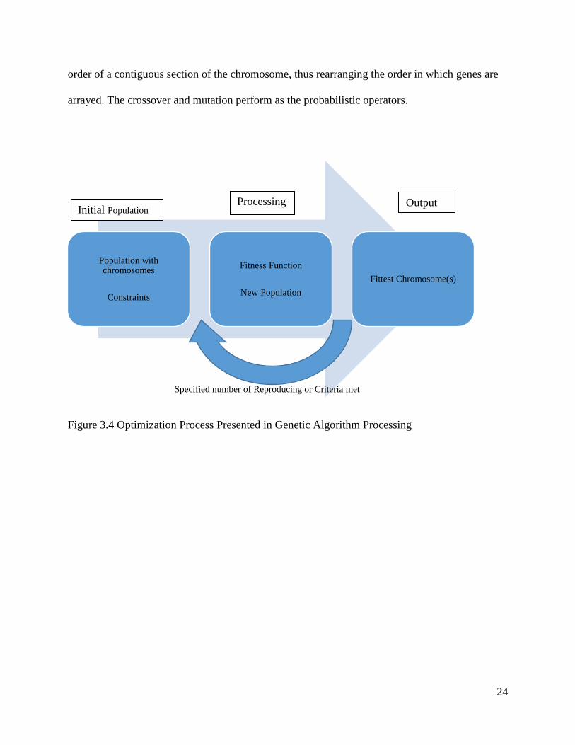
24
order of a contiguous section of the chromosome, thus rearranging the order in which genes are
arrayed. The crossover and mutation perform as the probabilistic operators.
Figure 3.4 Optimization Process Presented in Genetic Algorithm Processing
Population with chromosomes
Constraints
Fitness Function
New Population
Fittest Chromosome(s)
Initial Population Processing Output
Specified number of Reproducing or Criteria met

25
4. Execution of Genetic Algorithm Optimizer in CMG STARS Environment
4.1 Methodology and Model Details
The base model used a Cartesian grid type with dimensions of 120 x 16 x 50 in the I, J, and K
directions, respectively. The grid length in the I and J directions are 5 m and 50 m, respectively;
and the grid thickness in the K direction was 1 m. The total number of blocks was 96,000, and
only one well pair was used for SAGD production and SA-SAGD production.
The matrix properties were summarized below:
• Porosity: 0.3
• Permeability in I, J, K directions: 6000 md, 6000 md and 4800 md
• Temperature: 20 °C
• Water Saturation: 0.20
• 3 shale layers that lay at 267 m, 272 m and 283 m depth in layer 18, layer 23, and layer
34, respectively
The well pair is located in the middle of the reservoir in the I direction. The injector is located at
294 m depth (layer 45 in the K direction) and the producer is located 5 meters below the injector,
at 299 m TVD (layer 50 in the K direction). The injected steam temperature is 270.112°C with
1.0 steam quality.
The well constraint for the injector is 5500 kPa (maximum bottom hole pressure), and the well
constraint for the producer is 1500 m3/day of surface liquid production and 400 m3/day of a
steam rate. Before SAGD and SA-SAGD production started on 2017/04/01, three months of a
preheating period were set up by using a heater well option. A 270.112oC wellbore temperature

26
is selected for both heater wells to preheat the well pair from 2017/01/01 to 2017/04/01. During
this period, the well pair was shut in. The purpose of preheating was to mobilize the oil at the
well pair and to establish a thermal communication between the producer and the injector. The
intervening fluid between the well pair was normally heated to a temperature sufficiently high to
trigger the oil flow from the injector to the producer.
After preheating, the SAGD and SA-SAGD production started on 2017/04/01 and ended on
2027/01/1. The entire simulation time is 10 years.
Figure 4.1 Description of the Reservoir
Heavy oil composition was simplified and was represented by only three heavy components, and
the Peng-Robinson equation of state was used. An injector well was defined at the top and a
producer well at the bottom of the model. The rates were kept small enough to be able to
27
maintain a fairly constant pressure, which was true for most experiments. An asphaltene effect
on flow dynamics was also modeled. In the case of heavy oil, asphaltene is generally stable and
does not create problems of permeability reduction of the porous media. However, in miscible
displacement, the oil undergoes a composition change and thus the thermodynamic equilibrium
needed for the stability of asphaltene is broken. As a result, asphaltene accumulates and makes
flocs. This process can be termed asphaltene flocculation and is reversible. Flocculation is
beneficial because it contributes to viscosity reduction of heavy oil, but can be troublesome at the
same time because it increases the chance of asphaltene precipitation in porous media. In
general, not all the asphaltene that was flocculated will also be precipitated. An attempt has been
made to model these processes using CMG STARS. It was also attempted to clarify the
difference between asphaltene flocculation, precipitation and deposition. A number of factors
were considered and engineering assumptions were made for modeling asphaltene.
4.2 The Pre-processing
The role of pre-processing is to introduce the genes, decode the alleles, and initialize the first
learning generation of chromosomes for the genetic optimization algorithm, which ensures that
the genetic algorithm optimizer mingles with optimum solutions over the learning generations.
The selection criteria that secure the fitter chromosomes are associated with higher opportunities
for reproducing depends on the fitness of parent chromosomes.
In general, the values of parameters can be defined with either the discrete values for the binary
genetic algorithm or a range with minimum and maximum values for both binary and continuous
genetic algorithms. The binary genetic algorithm employs binary strings to exhibit an allele.
Thanks to the advantage of the analogy between a binary genetic algorithm and biological

28
evolutions, a binary genetic algorithm has been chosen for the process. A quantization technique
converts continuous values into binary and vice versa. The quantization technique uses a part of
a continuous range of values and then categorizes these samples into non-overlapping sub-
ranges, and each sub-range is associated with a specific discrete value. Haupt and Haupt (2004)
presented mathematical formulas for binary encoding and decoding of the nth variable.
For encoding,
𝑃𝑛𝑜𝑟𝑚=𝑃𝑛−𝑃𝑙𝑜𝑤
𝑃ℎ𝑖−𝑃𝑙𝑜𝑤
𝑔𝑒𝑛𝑒[𝑚] = 𝑐𝑒𝑖𝑙 {𝑃𝑛𝑜𝑟𝑚 − 2−𝑚 − ∑ 𝑔𝑒𝑛𝑒[𝑃]
𝑚−1
𝑃=1
2−𝑃}
For decoding,
𝑃𝑞𝑢𝑎𝑛𝑡 = ∑ [𝑚]
𝑁𝑔𝑒𝑛𝑒
𝑚=1
2−𝑚 + 2−(𝑀+1)
𝑞𝑛 = 𝑃𝑞𝑢𝑎𝑛𝑡 (𝑃𝑚 − 𝑃𝑙𝑜𝑤) + 𝑃𝑙𝑜𝑤
In each case, 𝑃𝑛𝑜𝑟𝑚 = normalized variable, where 0 ≤ 𝑃𝑛𝑜𝑟𝑚 ≤ 1.
Notation:
Plow = smallest variable value
Phi = highest variable value
gene[m] = binary version of Pn
ceil{x} = smallest integer not less than x
Pquant = quantized version of Pnorm
qn = quantized version of Pn
Ngene = number of bits of a gene
M = total number of bits of a gene

29
Initially, the objective function evaluates the first population of chromosomes according to the
criteria. In the circumstance of reservoir simulation, the chromosomes are the input files
containing parameter values. In order to inform the simulator to identify the optimization
parameters, the parameters are defined both in a parameter file and in the input file for the
simulator.
Once the fitness for all the chromosomes are evaluated, the genetic algorithm does selection,
crossover and mutation to generate the next learning generation of chromosomes; these functions
are the key components in a genetic algorithm to determine how good and how fast the solutions
converge to the optimum ones over the learning generations. Apart from selecting parent
chromosomes, performing the crossover and mutation, and generating the child chromosomes to be
submitted to the reservoir simulators, an optimization tool is the crucial part in the entire process to
determine the speed and accuracy of convergence to the optimum solutions. Selection is the step of
choosing chromosomes as the parents for generating the offspring. The rank represents the
fitness of the chromosomes from the highest to the lowest. Not all the chromosomes will survive
for crossover; the selected chromosomes, the selection rate X, is the fraction of the population.
Thus the number of chromosomes kept for each learning generation is called an X rate N pop.
The remaining, or the rate equaling 1-Xrate, N pop chromosomes for each learning generation,
will be from the crossover. That letting only a few chromosomes survive limits the available
genes in the offspring, and keeping too many chromosomes allows the unfit chromosomes to
contribute their traits to the next learning generation. 50% is a typical X rate in natural processes.
The most popular selection method for the genetic algorithm is the Roulette Wheel selection
method. The fundamental of the method is by defining that the probabilities of the chromosomes
for crossover are proportional to their fitness. A chromosome with the lowest fitness has the
lowest probability for crossover, and accordingly, a chromosome with the highest fitness has the

30
greatest probability for crossover. The ranking weighting is problem-independent and derives the
probability from the rank n of a survived chromosome (Nkeep represents the number of survivals).
𝑃𝑛 = 𝑁𝑘𝑒𝑒𝑝 − 𝑛 + 1
∑ 𝑛𝑁𝑘𝑒𝑒𝑝
1
In the case of fitness weighting, the probability of selection is calculated from the fitness rather
than a chromosome’s rank in the population.
𝑃𝑛 = |𝑓𝑛
∑ 𝑓𝑚𝑁𝑘𝑒𝑒𝑝𝑚=1
|
Crossover is the method for creating one or more offspring from the parents from the selection
process. The most common method of crossover involves two parents that produce two
offspring.
In order to demonstrate the overall process of crossover in general, the single-point crossover
method is employed. In a single-point crossover process, a crossover point is randomly selected
between the first and the last bits of the parents’ chromosomes. Parent number 1 passes one of
genes, its binary code, to offspring number 2; and parent number 2 passes one of its binary codes
to the same crossover point to offspring number 1. The offspring inherits portions of binary code
from both parents. This single-point crossover has been recognized as a representative and
effective crossover method.
Gene Gene Gene Gene Gene
Parent Chromosome 1 01110000010 1111101000 1000100111 10110111011 11101000010
Parent Chromosome 2 11111000111 1001000010 1110011110 10000100111 11110111000
Child Chromosome 1 01110000010 1001000010 1000100111 10110111011 11101000010
Child Chromosome 2 11111000111 1111101000 1110011110 10000100111 11110111000
Table 4.1: The single-point crossover method in genetic algorithm (Al-Gosayir et al. 2011a).

31
Mutation is the method of altering a certain percentage of the bits in the list of chromosomes.
Mutation introduces traits not in the original population and keeps the GA from converging too
fast before sampling the entire variable space. Mutation assures that the solutions more likely
converge to global optimum solutions instead of local optimum solutions. A higher number of
mutations means a higher freedom for the Algorithm to search variables outside of the current
range.
In this thesis, a technology called Elitism that disallows mutation is employed, since it is a quite
common practice in order not to ignore a perfect learning generation.
4.3 Implementation of Optimization Process
In the same fashion, the genetic algorithm starts with determining the optimization variables,
specifying the objective function, and defining the fitness. In this thesis, the objective function
depends on the outputs from reservoir simulation by solving a set of highly nonlinear mass
balance, momentum balance (Darcy’s law), and energy balance equations; and it is not
analytically delineated. As such, the genetic algorithm is an effective approach for reservoir
simulation optimization since the objective function is highly nonlinear. Like other optimization
techniques, the process finishes by validating the convergence criteria.
In this thesis, an optimization tool based on the Genetic Algorithm is coded in programming
language Python. This optimization tool then joins the reservoir simulator (CMG STARS) to
perform computing.
The process consists of three main components. A pre-processing, the execution, and a post-
processing. The role of pre-processing is to introduce the genes, decode the alleles, and initialize
the first learning generation of chromosomes for the genetic optimization algorithm. The
32
execution that begins with the design of the optimization tool is the main component. The role of
the tool is to select parent chromosomes, perform the crossover and mutation, and generate the
child chromosomes for the reservoir simulators to compute. The design of this tool determines
the speed and accuracy of convergence to the optimum solutions. The last component is the post-
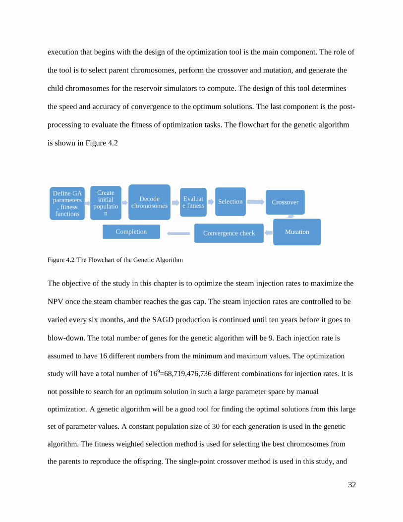
processing to evaluate the fitness of optimization tasks. The flowchart for the genetic algorithm
is shown in Figure 4.2
Figure 4.2 The Flowchart of the Genetic Algorithm
The objective of the study in this chapter is to optimize the steam injection rates to maximize the
NPV once the steam chamber reaches the gas cap. The steam injection rates are controlled to be
varied every six months, and the SAGD production is continued until ten years before it goes to
blow-down. The total number of genes for the genetic algorithm will be 9. Each injection rate is
assumed to have 16 different numbers from the minimum and maximum values. The optimization
study will have a total number of 169=68,719,476,736 different combinations for injection rates. It is
not possible to search for an optimum solution in such a large parameter space by manual
optimization. A genetic algorithm will be a good tool for finding the optimal solutions from this large
set of parameter values. A constant population size of 30 for each generation is used in the genetic
algorithm. The fitness weighted selection method is used for selecting the best chromosomes from
the parents to reproduce the offspring. The single-point crossover method is used in this study, and
Define GA parameters
, fitness functions
Create initial
population
Decode chromosomes
Evaluate fitness
Selection Crossover
MutationConvergence check Completion

33
the crossover rate is set to be 75%. The mutation rate is 25%, and the rate for elitism is 10%. These
genetic algorithm parameters are by no means the best, and the sensitivities of the genetic algorithm
parameters are studied in next chapter.
4.4 The post-processing
This is a process to evaluate the fitness of the chromosomes that are outputs of execution of
optimization tools. To acquire the chromosomes that have the highest fitness is the ultimate goal
of the optimization. Fitness is also a device to determine the ranking of chromosomes in the
current learning generation. The selection method depends on the ranking of the population in
the current learning generation. Fitness can be a simple analytical function, or a function
dependent on the variables from highly nonlinear systems. In this thesis, the fitness is a function
on the variables from the simulation results generated from the reservoir simulators. The fitness
functions commonly adopted in evaluating the SAGD and SA-SAGD performance are the
cumulative steam to oil ratio (CSOR) and some economics indictors like the net present value
(NPV). Another important role of post-processing is to check the convergence of a genetic
algorithm. There is no standardized convergence criteria in a genetic algorithm, and researchers
may use a fixed number of learning generations as the indication of meeting criteria, or use the
achieving of an acceptable solution as the indication. Most genetic algorithms keep track of the
population statistics in the form of a population mean, population distribution, and maximum
fitness. For instance, these two occasions of reaching an optimal solution are widely accepted:
one is when the mean of the fitness among the population does not improve more than a
tolerance over the neighboring of two learning generations; the other is when a large fraction of
the population’s fitness is within the tolerance of the best chromosome’s fitness in one learning
generation.

34
4.5 Comparison with a Gradient-based Method
In this section, the genetic algorithm optimization tool executed in this work is compared with
one of the gradient-based optimization methods. Gradient-based optimization methods have been
widely used in the optimization industry. Nevertheless, those methods require the values of
derivatives of fitness functions with regard to parameters, which in many cases are difficult to
obtain. The gradient-based methods also have the disadvantage of converging to the local
optimum solutions instead of global ones. The backpropagation (BP) method, as one of one
popular gradient-based methods, acts as the contrast in this thesis for the purpose of comparison
with genetic algorithm optimization.
4.5.1 The backpropagation method
The popularity of the BP method is associated with the wide availability of commercial software,
such as Matlab Neural Network Toolbox. By calculating the gradient information of an error
function and propagating it backwards, the method optimizes the weights. The weights adjust
along with the direction, which minimizes the output error. The BP method is commonly referred
as a trajectory-driven approach by performing a local search (Montana et al. 1989). The
disadvantage of the method is that the algorithms may be trapped at local optima of an error
function if the initial values are set inappropriately.
4.5.2 The comparison
Unlike BP as a trajectory-driven approach, a Genetic Algorithm is a population-driven approach
by performing a global search to find the near optimal solution from a large and complex space
(Montana et al. 1989). A short literature review has been listed below:
35
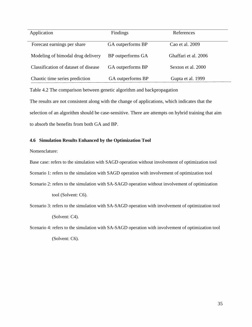
Application Findings References
Forecast earnings per share GA outperforms BP Cao et al. 2009
Modeling of bimodal drug delivery BP outperforms GA Ghaffari et al. 2006
Classification of dataset of disease GA outperforms BP Sexton et al. 2000
Chaotic time series prediction GA outperforms BP Gupta et al. 1999
Table 4.2 The comparison between genetic algorithm and backpropagation
The results are not consistent along with the change of applications, which indicates that the
selection of an algorithm should be case-sensitive. There are attempts on hybrid training that aim
to absorb the benefits from both GA and BP.
4.6 Simulation Results Enhanced by the Optimization Tool
Nomenclature:
Base case: refers to the simulation with SAGD operation without involvement of optimization tool
Scenario 1: refers to the simulation with SAGD operation with involvement of optimization tool
Scenario 2: refers to the simulation with SA-SAGD operation without involvement of optimization
tool (Solvent: C6).
Scenario 3: refers to the simulation with SA-SAGD operation with involvement of optimization tool
(Solvent: C4).
Scenario 4: refers to the simulation with SA-SAGD operation with involvement of optimization tool
(Solvent: C6).

36
Figure 4.3 Accumulative Steam-Oil Ratio Chart
Figure 4.4 Accumulative Water SC Chart

37
Figure 4.5 Base Case
Figure 4.6 Scenario 1

38
Figure 4.7 Scenario 2
Figure 4.8 Scenario 3

39
Figure 4.9 Scenario 4
NPV calculations for SAGD operation:
NPV = (cumulative oil × oil price) × (1 - discount rate) - current year × annual operating cost -
numbers of pairs × (operation cost per pairs) - cumulative water × water treatment - cumulative
injection water × water injection cost - cost of surface facility - numbers of wells × cost of
drilling and completion
Oil price $100/STB
Discount rate 4%
Annual operating cost $400,000
Operation cost per producer $100,000
Operation cost per injector $50,000
Water treatment $ 0.25/STB
Water injection cost $ 2/STB
Cost of surface facility $400 MM
Cost of drilling and completion of a horizontal well $15 MM
Table 4.3 The parameters for NPV calculations in the SAGD process

40
NPV calculation for SA-SAGD operation:
NPV = (cumulative oil × oil price) × (1 - discount rate) - current year × annual operating
cost -numbers of pairs × (operation cost per pairs) - cumulative water × water treatment -
cumulative injection water × water injection cost –cost of solvent- cost of surface facility -
numbers of wells × cost of drilling and completion
Table 4.4 The Parameters for NPV calculations in the SA-SAGD process
Cumulative
Oil Produced
MM STB
Cumulative
Water
Produced
MM STB
Cumulative
Water
Injected
MM STB
Cumulative
Steam Oil
Ratio RF (%)
NPV
($ MM)
Base case 0.943 3.233 3.487 3.696 16.845 86.5
Scenario 1 1.097 5.268 5.652 5.152 19.589 149.0
Scenario 2 0.333 5.270 5.300 4.827 5.946 -308.0
Scenario 3 0.980 4.966 5.227 5.330 17.509 142.0
Scenario 4 1.137 3.847 4.131 3.632 20.31 194.6
Table 4.5 Summary of the NPV calculations
Summary
In this chapter, an optimization tool using a genetic algorithm is designed and implemented. The
design of the genetic algorithm tool is divided into three parts: the pre-processor, the optimizer
and the post-processor. The pre-processor of a genetic algorithm optimizer facilitates performing
Oil price $60/STB
Discount rate 4%
Annual operating cost $400,000
Operation cost per producer $100,000
Operation cost per injector $50,000
Water treatment $ 0.25/STB
Water injection cost $ 2/STB
Cost of surface facility $400 MM
Cost of Solvent $100 MM
Cost of drilling and completion of a horizontal well $15 MM

41
optimization tasks automatically. It processes the parameters and initializes the first learning
generation of chromosomes in the genetic algorithm optimization. The optimizer is the key part
to determine how well and how fast the genetic algorithm converges to an optimum. The
selection method is used to select the chromosomes for reproduction; the crossover method
determines how the offspring is reproduced from parents; and the mutation method alters a
certain percentage of the bits in the list of chromosomes to ensure that the genetic algorithm has
a better chance converging to a global optimum. The post-process is used to evaluate the
optimization objective functions and rank the fitness. The genetic algorithm optimizer is
compared with a gradient-based optimization method using some benchmark problems to verify
its validity and superiority.

42
5 Conclusions and Recommendations on Future Work
The optimization tool is incorporated with the numerical reservoir simulator (CMG STARS) to
perform the optimization in the SAGD process and SA-SAGD process separately. The objective
for the optimization study in this thesis is to optimize the steam injection rates in the SAGD
process after the steam chamber reaches the overburden. The net present value is used as an
objective function. The economics of the SAGD process is based on the output from numerical
simulations. The genetic algorithm implemented facilitates the convergence to the global optimal
solutions. The sensitivities of the genetic algorithm parameters are also studied.
In this thesis, the genetic algorithm is successfully applied for production optimization in the
SAGD process and SA-SAGD operations. It is noted that all the conclusions are only applicable
to the specific reservoir conditions that are depicted in Chapter 4. The optimum steam injection
rates are identified with the genetic algorithm. The attempt was to use high pressure injection at
the beginning of the SAGD process to maximize the oil rate and to facilitate rapid steam
chamber development. After the steam breakthrough to the overburden, high steam injection
rates can be maintained for a period until the steam chamber is fully expanded. Although
operating at high rates is associated with heat loss to the overburden, the oil production has been
maximized with the high injection rate. It is more economically viable to compromise heat loss
to the overburden in the process than to decrease the steam injection rates immediately after
steam breakthrough.
5.1 Conclusions
From this thesis, a set of preliminary conclusions can be drawn as follows:

43
1. The genetic algorithm, as one of the evolutionary optimization methods, may be a viable
solution to identify a global optimal solution, though this may only be applicable to the particular
reservoir stated in Chapter 4. Apart from less cost on computation, the genetic algorithm is more
convenient to be implemented than the gradient-based methods, since there is no involvement of
any derivative operation. It can handle arbitrary kinds of constraints and objectives. The
comparison between the genetic algorithm and backpropagation optimization method discloses
that the genetic algorithm may converge to a global optimal solution more quickly than the
gradient-based method, and the genetic algorithm has the advantage of avoiding confinement to a
local optimal solution.
2. The research has performed an optimization process by the Genetic Algorithm in a simulated
environment, together with the application of commercial software. The process and the
simulation results indicate the possibility of standardizing the process, parameter setting and
simulation results on a condition that the computation power has been trained to understand the
objective function. In this thesis, the parameters to be optimized are the steam injection rates
changing every six months of SAGD (SA-SAGD) production after the steam chamber reached
the overburden. The optimal injection rates setting identified by the genetic algorithm is to use
the high steam injection rate initially and then gradually to increase the steam injection rates until
the occasion when the steam chamber reaches the horizontal boundary of the reservoir. Followed
by the reduction of the steam injection rates, the lower injection rates will be in the charge until
to the late stage of the process. Although the finding may be only applicable to the particular
reservoir, it is worth noting that the machine learning practice may help reservoir engineers to
identify the best parameter setting quickly and effectively.

44
3. The laboratory environment hardly mimics the real reservoir conditions; one of the
disadvantages is the low-pressure circumstance. In the real reservoir situation, the high pressure
will cause a much faster condensing speed of gaseous solvent, which derives a slow diffusion
process. Hence, due to the inability of developing into a quick diffusion phase, the low initial
production rate represents the key issue in the SA-SAGD process. The other typical challenge is
that high bitumen precipitation may cause decreasing permeability that derives a lower ultimate
oil recover rate. Although the selection of the solvent and the design of the operation parameters
can compensate the drawbacks partially, it is still a wide open discussion across industry and
research institutions on the systematic approach to design and monitor the SA-SAGD recovery
process; therefore, SA-SAGD has not been widely accepted as a promising extraction process.
4. In this thesis, the fitness weighting selection method generates a more effective result than the
ranking weighting method. The ranking weighted method may not be effective for this particular
reservoir condition. The uniform crossover method is not as good as other crossover methods
since it introduced too much randomness.
5. The impact of a population size adopted in the genetic algorithm can be negligible. The
difference brought by various population sizes on fitness comparison is insignificant, although
the ideal population size in the genetic algorithm is found to be around 35-55 using the SAGD
process optimization problem studied in this thesis.
6. Elitism copies the most fitted chromosomes to the next generation from the current generation.
The effect of elitism on the convergence of the genetic algorithm is observed in this thesis. The
genetic algorithm converges more slowly without elitism. An ideal elitism rate for SAGD
optimal operation in this thesis was about 10%.

45
7. Nonlinear response surface proxy can potentially offer a more accurate representation of the
true objective function value, although this technique is also inclined to over-shoot during
extrapolation. Therefore, a periodic updating scheme is proposed. The implementation of this
step delivers the improved predictability of the objective function, although a minimal increase
in computational time is observed.
8. The crossover process in the genetic algorithm determines the percentage of the specific
parent chromosomes conveyed to the chromosomes of the next generation. In order to assure that
the optimal solution identified by the genetic algorithm can play a role in improving the fitness
of next generations, a large amount of the unfit chromosomes in the current generation does not
participate into the crossover process. A higher crossover rate even generates a quicker
evolvement of fitness of next generations. However, there is a limit in terms of the crossover rate
to reflect the essence of the genetic algorithm. A 100%, though it is the highest in theory, cannot
be the parameter in the study. Instead, a 70% crossover rate may be a more feasible solution.
9. Mutation, as another methodology to improve the fitness of next generation, can prohibit the
chromosomes falling into the trap of local extrema by performing the random changes of the
offspring’s chromosomes. A relatively high mutation rate indicated that the genetic algorithm
goes to random search that is sometimes uncontrollable. Therefore, a moderate mutation rate
generates the best possible result. An ideal mutation rate around 1% can be the optimal.
10. The impact brought by the various types of solvents was also observed in this thesis. By
concluding that C6 was associated with higher SGAD performance than C4, it was only an
indicative denouement that may not be applicable for a different reservoir condition.

46
5.2 Recommendations
A number of research directions can be suggested based on this thesis:
1. The optimization technique may only be effective on the specified reservoir conditions. In
order to apply the technique or techniques into more reservoir conditions, a similar approach on
typical reservoirs shall be conducted. Eventually, the generalization of reservoir conditions
coupled by the effectiveness of various optimal techniques will bring the conception into
industrial practice.
2. This study only covers the SAGD and SA-SAGD processes with one type of reservoir. More
recovery techniques on heavy oil shall be studied. The computational efficiency of the technique
allows optimization to be carried out successfully for heterogeneous reservoirs. These case
studies illustrated that the hybrid optimization framework is a useful tool for designing complex
recovery processes and increasing the profit.
3. From the perspective of programming, the comparison between a continuous genetic
algorithm and a binary genetic algorithm shall be conducted in future work. In this thesis, the
binary approach mimics the biological evolution process in the best possible way; nevertheless,
since the need of decoding of chromosomes prior to the assessment of the fitness function
requires significant extra computation power and time, the floating-point values representation
shall be taken into account. Particularly, the variable parameters are continuous.
4. The selection of various types of solvents shall be observed in future, since the impact brought
by interactions between hydrocarbon components and solvents is significant for heavy oil
recovery.

47
5. The multiple-objective optimization technique shall be studied for reservoir simulation
practice, since there are always conflicting priorities in most of the reservoirs recovery processes.
In this thesis, a Net Present Value has been set with the top priority; nevertheless, other
evaluation parameters, such as water usage and steam-oil-ratio, are also crucial. Zitzler and
Thiele (1999) compared the performance of various multiple-objective genetic algorithms. A
balanced approach to identify the optimal recovery process by setting the weights of various
objectives shall be considered in future wok.
6. In the real world, it is usually extremely hard to identify the unique global optimal solution.
The ideal optimization method normally predetermines a reasonable number of iterations. It
hardly can have a conclusion that the perfect time can be determined after a certain number of
iterations.
In future work, several possibilities shall be considered to optimize the SAGD process:
a) Check the best chromosome for each generation to see if it is an acceptable answer to the
problem. Stop the algorithm if it is.
b) If the genetic algorithm continues with the same best chromosome for a certain number of
generations, then stop the genetic algorithm.
c) If the mean or standard deviation of the population’s fitness reaches a certain level, then stop
the genetic algorithm.
d) Limit the maximum number of iterations.
Criterion c) has been used in this thesis. Nevertheless, the other three approaches are quite
important to be carried into the future studies. Furthermore, if the future work may disclose the

48
best possible approach on the iteration criterion for SAGD process that will be a quite helpful
finding.
7. The comparison between proxy modelling and genetic algorithms shall be undertaken to
balance the accuracy and computing speed. The proxy modelling enables a faster computation; it
is usually inaccurate compared with genetic algorithms.
8. A pilot project in the field may also be considered given that the further lab work provides
promising simulation results. The field development optimization, well completion optimization
and history matching can also be incorporated into the research.
9. The SAGD simulation model used in this thesis is a simplified 3D model, which assumes the
uniform distribution of a steam chamber along a wellbore. In reality, the impact of pressure and
heat transfer losses along the horizontal section of a SAGD well can significantly impair the
distribution and efficiency of its steam chamber from bottom to top. A more complex 3D model
may be taken into account to simulate real-world problems better.
-END-

49
REFERENCES
AlBulushi, N., King, P. R., Blunt, M. J., Kraaijveld, M. 2009. Development of artificial neural
network models for predicting water saturation and fluid distribution. J. Pet. Sci. Eng., vol.
68, no. 3–4, pp. 197–208, Oct.
AlDousari, M. M., Garrouch, A. A. 2013. An artificial neural network model for predicting the
recovery performance of surfactant polymer floods. J. Pet. Sci. Eng., vol. 109, pp. 51–62,
Sep.
Ali Ahmadi, M., Zendehboudi, S., Lohi, A., Elkamel, A., Chatzis, I. 2013. Reservoir
permeability prediction by neural networks combined with hybrid genetic algorithm and
particle swarm optimization. Geophys. Prospect., vol. 61, no. 3, pp. 582–598, May.
Ali, M. M., Jagadeesh, P. S. V., Lin, I.I., Hsu, J.Y. 2012. A neural network approach to estimate
tropical cyclone heat potential in the Indian Ocean. IEEE Geosci. Remote Sens. Lett., vol. 9,
no. 6, pp. 1114–1117, Nov.
Aminian, K., Ameri, S. 2005. Application of artificial neural networks for reservoir
characterization with limited data. J. Pet. Sci. Eng., vol. 49, no. 3–4, pp. 212–222, Dec.
Asadi, S., Shahrabi, J., Abbaszadeh, P., Tabanmehr, S. 2013. A new hybrid artificial neural
networks for rainfall–runoff process modeling. Neurocomputing, vol. 121, pp. 470–480,
Dec.
Auda, G., Kamel, M. 1999. Modular neural networks: a survey. Int. J. Neural Syst., vol. 9, no. 2,
pp. 129–51, Apr.
Belgrave, J.D.M., Nzekwu, B., Chhina, H.S. 2007. SAGD Optimization with Air Injection. Paper
SPE 106901, SPE Latin American and Caribbean Petroleum Engineering Conference,
Buenos Aires, Argentina, 15-18 April.
Bittencourt, A.C., Horne, R.N., 1997. Reservoir Development and Design Optimization. Paper
SPE 38895 presented at the 1997 SPE Annual Technical Conference and Exhibition held in
Antonio, Texas, 5-8 October.

50
Butler, R.M., Mokrys, I.J. 1989. Solvent analog model of steam-assisted gravity drainage.
AOSTRA J. Res., 5 (1):17–32.
Butler, R.M., Mokrys, I.J. 1991. A New Process (SA-SAGD) for Recovering Heavy Oils Using
Hot Water and Hydrocarbon Vapour. Journal of Canadian Petroleum Technology 30 (1):
97-106.
Chaki, S., Verma, A. K., Routray, A., Mohanty, W. K., Jenamani, M. 2014. Well tops guided
prediction of reservoir properties using modular neural network concept: a case study from
western onshore, India. J. Pet. Sci. Eng., vol. 123, pp. 155 – 163, Jul.
Colin, C., Chakrabarty, N. and Gates, I.D. 2006. Automated Global Optimization of Commercial
SAGD Operations. Paper 2006-157, Canadian International Petroleum Conference, Calgary,
AB, 13-15 June.
Cao, Q., Parry, M. E. 2009. Neural network earnings per share forecasting models: A
comparison of backward propagation and the genetic algorithm. Decision Support Systems,
vol. 47, pp. 32-41.
Chen, Z. 2007. Reservoir Simulation: Mathematical Techniques in Oil Recovery. Society for
Industrial and Applied Mathematics, Philadelphia, PA.
Das, S.K. and Butler, R.M. 1996. Countercurrent Extraction of Heavy Oil and Bitumen. Paper
SPE 37094 presented at the SPE International Conference on Horizontal Well Technology,
Calgary, Canada. 18-20 November. DOI: 10.2118/37094-MS.
Ding, Y., Feng, Q., Wang, T., Fu, X. 2014. A modular neural network architecture with concept.
Neurocomputing., vol. 125, pp. 3–6, Feb.
Edmunds, N., Moini, B. and Peterson, J. 2009a. Advanced Solvent-Additive Processes via
Genetic Optimization. Paper PETSOC 2009-115 presented at Canadian International
Petroleum Conference (CIPC) 2009, Calgary, Alberta, Canada. 16-18 June.
Edmunds, N., Riva, J. and Peterson, J. 2010. Engineering Aspects of Solvent-Additive Steam
Recovery. World Heavy Oil Development Seminar, Panjin, China, September 15-17.

51
Eren, H., Fung, C. C., Wong, K. W. 1997. Modular artificial neural network for prediction of
petrophysical properties from well log data. IEEE Trans. Instrum. Meas., vol. 46, no. 6, pp.
1295–1299, Dec.
España-Boquera, S., Castro-Bleda, M. J., Gorbe-Moya, J., Zamora-Martinez, F. 2011. Improving
offline handwritten text recognition with hybrid HMM/ANN models. IEEE Trans. Pattern
Anal. Mach. Intell., vol. 33, no. 4, pp. 767–779, Apr.
Friedrich, K. 2005. Effects of a Non-Condensable Gas on the SA-SAGD Process. M.Sc
dissertation, University of Waterloo, Waterloo, Ontario, Canada.
Gates, I. D. and Chakrabarty, N. 2005. Optimization of Steam-Assisted Gravity Drainage in
McMurray Reservoir. Paper 2005-193, Canadian International Petroleum Conference,
Calgary, AB, June 7-9.
Gates, I. D. and Chakrabarty, N. 2006. Design of the Steam and Solvent Injection Strategy in
Expanding-Solvent Steam-Assisted Gravity Drainage. Paper 2006-023, Canadian
International Petroleum Conference, Calgary, AB, June 13-15.
Gates, I. D., Kenny, J., Hernandez-Hdez, I.L. and Bunio, G.L. 2007. Steam-Injection Strategy
and Energetics of Steam-Assisted Gravity Drainage. SPE Reservoir Evaluation &
Engineering, pp. 19-34, February.
Ghaffari, A., Abdollahi, H., Khoshayand, M. R., Bozchalooi, I. S., Dadgar, A, Rafiee Tehrani,
M. 2006. Performance comparison of neural network training algorithms in modeling of
bimodal drug delivery. International Journal of Pharmaceutics, vol. 327, pp.126-138.
Giacchettaa, G., Leporinia, M., Marchettib, B. 2015. Economic and environmental analysis of a
Steam Assisted Gravity Drainage (SAGD) facility for oil recovery from Canadian oil sands.
Applied Energy 142 (3): 1-9.http://dx.doi.org/10.1016/j.apenergy.2014.12.057.
Government of Alberta, 2014. Retrieved from: http://www.energy.alberta.ca/OilSands/791.asp
Govind, P., Das, S., Srinivasan, S. and Wheeler, T.J. 2008. Expanding Solvent SAGD in Heavy
Oil Reservoirs. Paper SPE/PS/CHOA 117571 presented at the 2008 SPE International
Thermal Operations and Heavy Oil Symposium, Calgary, Alberta, Canada, 20-23 October.
DOI: 10.2118/117571-MS.

52
Gupta, J. N. D., Sexton, R. S. 1999. Comparing backpropagation with a genetic algorithm for
neural network training. Omega, vol.27, pp. 679-684.
Gupta, S., Gittins, S.D. 2012. An investigation into Optimal Solvent Use and the Nature of
Vapor/Liquid Interface in Solvent-Aided SAGD Process with a Semi-analytical Approach.
SPE.J. 17 (4): 1255-1264. SPE – 146671-PA. http://dx.doi.org/10.2118/146671.PA.
Hampson, D. P., Schuelke, J. S., Quirein, J. A. 2001. Use of multiattribute transforms to predict
log properties from seismic data. Geophysics., vol. 66, no. 1, pp. 220–236, Jan.
Holland, J. H. 1975. Adaptation in Natural and Artificial Systems. University of Michigan Press.
(Second edition: MIT Press, 1992.)
Ivory, J., Zheng, R., Nasr, T., Deng, X., Beaulieu, G. and Heck, G. 2008. Investigation of Low
Pressure SA-SAGD. Paper SPE 117759 presented at the SPE International Thermal
Operations and Heavy Oil Symposium, Calgary, Alberta, Canada, 20-23 October. DOI:
10.2118/117759-MS.
Japan Canada Oil Sands Limited (JACOS). 2009. Hangingstone SAGD Demonstration 2008,
Project Thermal In-Situ Scheme Progress Report. Approval No. 8788G presented to the
Energy Resources Conservation Board, Calgary, Alberta, Canada. 23 March.
http://www.ercb.ca/docs/products/osprogressreports/2009/2009AthabascaJACOSHangingst
oneSAGD8788.pdf.
Jia, X., Cunha, L.B. and Deutsch, C.V. 2006. Investigation of a Stochastic Optimization Method
for Automatic History Matching of SAGD Processes. Paper 2006-190, Canadian
International Petroleum Conference, Calgary, AB, 13-15 June.
Jiang, N., Zhao, Z., Ren, L. 2003. Design of structural modular neural networks with genetic
algorithm. Adv. Eng. Softw., vol. 34, no. 1, pp. 17–24, Jan.
Kaydani, H., Mohebbi, A., Baghaie, A. 2012. Neural Fuzzy System Development for the
Prediction of Permeability From Wireline Data Based on Fuzzy Clustering. Pet. Sci. Eng.,
vol. 30, no. 19, pp. 2036–2045, Jul.
Kaastra, I., Boyd, M. 1996. Designing a neural network for forecasting financial and economic
time series. Neurocomputing., vol. 10, pp. 215–236.

53
Keshavarz, M., Okuno, R., Babadagli, T. 2014. Efficient Oil Displacement Near the CHAMBER
Edge in ES-SAGD. J. Petrol. Sci. Eng., 118 (June):99-113.
http://dx.doi.org/10.1016/j.petrol.2014.04.007.
Leaute, R.P. 2002. Liquid Addition to Steam for Enhancing Recovery of Bitumen with CSS:
Evolution of Technology from Research Concept to a Field Pilot at Cold Lake. Presented at
SPE International Thermal Operations and Heavy Oil Symposium and International
Horizontal Well Technology Conference. Calgary. Alberta. Canada. 4-7 November. SPE-
79011-MS. http://dx.doi.org/10.2118/79011-MS.
Leaute, R.P., Carey, B.S. 2005. Liquid Addition to Steam for Enhancing Recovery (LASER) of
Bitument with CSS: Results from the First Pilot Cycle. Presented at Canadian International
Petroleum Conference. Calgary. Alberta. Canada. 7-9 June. PETSOC-2005-161.
http://dx.doi.org/10.2118/2005-161.
Li, W., Mamora, D.D., Li, Y. 2011a. Light- and Heavy-Solvent Impacts on Solvent-Aided-
SADG Process; A Low-Pressure Experimental Study. Journal Canadian Petroleum
Technology 50 (4): 19-30. SPE-133277-PA. http://dx.doi.org/10.2118/133277.PA.
Lim, J.S. 2005. Reservoir properties determination using fuzzy logic and neural networks from
well data in offshore Korea. J. Pet. Sci. Engi., vol. 49, no. 3–4, pp. 182–192, Dec.
Melanie, M. 1999. An Introduction to Genetic Algorithms. 1st Ed., MIT Press, Massachusetts.
Mendoza, O., Melín, P., Castillo, O. 2009. Interval type-2 fuzzy logic and modular neural
networks for face recognition applications. Appl. Soft Comput. vol. 9, pp. 1377–1387, Sep.
Montana, D., Davis, L. 1989.Training feedforward neural networks using genetic algorithms.
Presented in 11th Int. Joint Conf. Artificial Intelligence, pp. 762-767.
Narayanan, K. and White, C.D.1999. Response Surface Methods for Upscaling Heterogeneous
Geologic Models. Paper SPE 51923, SPE Symposium on Reservoir Simulation, Houston,
Texas, 14-17 February.
Nasr, T.N., Ayodele, O.R. 2006. New Hybrid Steam-Solvent Processes for the Recovery of
Heavy Oil and Bitumen. Presented at Abu Dhabi International Petroleum Exhibition and

54
Conference. Abu Dhabi. UAE. 5-8 November. SPE-101717-MS.
http://dx.doi.org/10.2118/101717-MS.
Nenniger, J.E. and Dunn, S.G. 2008. How Fast is Solvent Based Gravity Drainage. Paper
PETSOC 2008-139 presented at the Canadian International Petroleum Conference/SPE Gas
Technology Symposium 2008 Joint Conference, Calgary, Alberta, Canada. 17-19 June.
DOI: 10.2118/2008-139.
Nikravesh, M., Aminzadeh, F. 2001a. Past, present and future intelligent reservoir
characterization trends. J. Pet. Sci. Engi., vol. 31, no. 2–4, pp. 67–79, Nov.
Nikravesh, M., Adams, R. D., Levey, R. A. 2001b. Soft computing: tools for intelligent reservoir
characterization (IRESC) and optimum well placement (OWP). J. Pet. Sci. Eng., vol. 29, pp.
239–262.
Nikravesh, M., Hassibi, M. 2003. Intelligent reservoir characterization (IRESC). IEEE Int.
Conference on Ind. Informatics, pp. 369–373.
Nikravesh, M. 2004. Soft computing-based computational intelligent for reservoir
characterization. Expert Syst. with Appl., vol. 26, no. 1, pp. 19–38, Jan.
Ostlin, E., Zepernick, H.J., Suzuki, H. 2010. Macrocell path-loss prediction using artificial neural
networks. IEEE Trans. Veh. Technol., vol. 59, no. 6, pp. 2735–2747, Jul.
Prada,V.J., Cunha,L.B., 2008. Prediction of SAGD Performance Using Response Surface
Correlations Developed by Experimental Design Techniques. Journal of Canadian
Petroleum Technology. 47(09) · September. DOI: 10.2118/2006-126.
Ray,S. 2015. Essentials of Machine Learning Algorithms. Retrieved from:
https://www.analyticsvidhya.com/blog/2015/08/common-machine-learning-algorithms.
Rogers, S. J., Fang, J. H., Karr, C. L., Stanley, D. A. 2014. Determination of lithology from well
logs using a neural network. Am. Assoc. Pet. Geol. Bull., vol. 76, pp. 731–739, 1992.
Sánchez, D., Melin, P. 2014. Optimization of modular granular neural networks using
hierarchical genetic algorithms for human recognition using the ear biometric measure. Eng.
Appl. Artif. Intell., vol. 27, pp. 41–56, Jan.

55
Sharma, N., Ali, M. M. 2013. A neural network approach to improve the vertical resolution of
atmospheric temperature profiles from geostationary satellites. IEEE Geosci. Remote Sens.
Lett., vol. 10, no. 1, pp. 34–37, Jan.
Singhal, A.K., Das, S.K., Leggitt, S.M., Kasraie, M. and Ito, Y. 1996. Screening of Reservoirs
for Exploitation by Application of Steam Assisted Gravity Drainage/SA-SAGD Processes.
Paper SPE 37144 presented at the International Conference on Horizontal Well Technology,
Calgary, Alberta, Canada. 18-20 November. DOI: 10.2118/37144.
Sivanandam, S.N., Deepa, S.N. 2008. Introduction to Genetic Algorithms. Springer-Verlag,
Berlin, Heidelberg.
Smaoui, N., Garrouch, A. A. 1997. A new approach combining Karhunen-Loeve decomposition
and artificial neural network for estimating tight gas sand permeability. J. Pet. Sci. Eng.,
vol. 18, pp. 101–112.
Snyman, J.A. 2005. Practical Mathematical Optimization: An Introduction to Basic Optimization
Theory and Classical and New Gradient-Based Algorithms. Springer Publishing, New York,
Sexton, R. S., Dorsey, R. E. 2000. Reliable classification using neural networks: a genetic
algorithm and backpropagation comparison. Decision Support Systems, vol. 30, pp. 11-22.
Upreti, S.R., Lohi, A., Kapadia, R, and El-Haj, R. 2007. Vapor extraction of heavy oil and
bitumen: A review, Energy and Fuels 21 (3): 1562-1574.
White, C.D. and Royer, S.A. 2003. Experimental Design as a Framework for Reservoir Studies.
paper SPE 79676, SPE Symposium on Reservoir Simulation, Houston, Texas, 3-5 February
Wong, P. M., Bruce, A. G., Gedeon, T. T. D. 2003. Confidence bounds of petrophysical
predictions from conventional neural networks. IEEE Trans. Geosci. Remote Sens., vol. 40,
no. 6, pp. 1440–1444, 2002.
Wong, P. M., Gedeon, T. D., Taggart, I. J. 1995. An improved technique in porosity prediction: a
neural network approach. IEEE Trans. Geosci. Remote Sens., vol. 33, no. 4, pp. 971–980,
Jul.

56
Yang, C., Card, C., Nghiem, L. 2009. Economic Optimization and Uncertainty Assessment of
Commercial SAGD Operations. Journal of Canadian Petroleum Technology, vol.48, No. 9,
pp. 33-40.
Yazdani, A., ALvestad, J., Kjonsvik, D. 2011. A parametric Simulation Study for Solvent Co-
injection Process in Bitumen Deposits. Presented at the Canadian Unconventional Resource
Conference. Calgary. Alberta. Canada.15-17 November. SPE-148804-MS. http://
dx.doi.org/10.2118/148804-MS.
Yeten, B., Castellini, A., Guyaguler, B. and Chen, W.H. 2005. A Comparison Study on
Experimental Design and Response Surface Methodologies. Paper SPE 93347, SPE
Symposium on Reservoir Simulation, Houston, Texas, 31 January-2 February.
Yu, S., Guo, X., Zhu, K., Du, J. 2010. A neuro-fuzzy GA-BP method of seismic reservoir fuzzy
rules extraction. Expert Syst. with Appl., vol. 37, no. 3, pp. 2037–2042, Mar.
Zerpa, L.E., Queipo, N.V., Pintos, S. and Salager, J.-L. 2004. An Optimization Methodology of
Alkaline-Surfactant-Polymer Flooding Processes Using Field Scale Numerical Simulation
and Multiple Surrogates. Paper SPE 89387, SPE/DOE 14th Symposium on Improved Oil
Recovery, Tulsa, Oklahoma, 17-21 April.
Zitzler, E. and Thiele, L. 1999. Multiobjective evolutionary algorithms: A comparative case
study and the strength pareto approach. IEEE Transactions on Evolutionary Computation,
3(4):257–271.
Zubarev, D.I. 2009. Pros and Cons of Applying Proxy-Models as a Substitute for Full Reservoir
Simulations. Paper SPE 124815, SPE Annual Technical Conference and Exhibition, New
Orleans, Louisiana, 4-7 October