Where computer vision needs help from computer science (and machine learning)
Regularization+
Neural Networks
1
10-601 Introduction to Machine Learning
Matt GormleyLecture 11
Feb. 20, 2019
Machine Learning DepartmentSchool of Computer ScienceCarnegie Mellon University

Reminders
• Homework 4: Logistic Regression
– Out: Fri, Feb 15
– Due: Fri, Mar 1 at 11:59pm
• Midterm Exam 1
– Thu, Feb 21, 6:30pm – 8:00pm
• Today’s In-Class Poll
– http://p11.mlcourse.org
• HW3 grades published
• Crowdsourcing Exam Questions
3

NON-LINEAR FEATURES
4
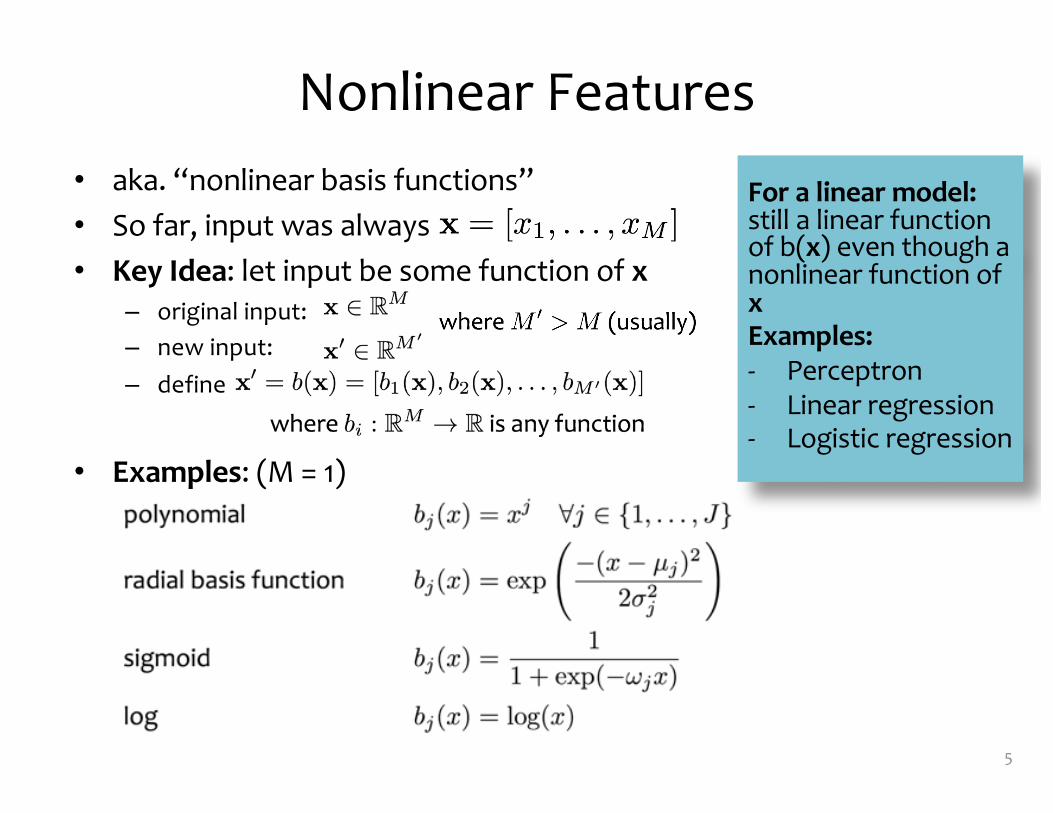
Nonlinear Features• aka. “nonlinear basis functions”• So far, input was always• Key Idea: let input be some function of x
– original input:– new input:– define
• Examples: (M = 1)
5
For a linear model: still a linear function of b(x) even though a nonlinear function of xExamples:- Perceptron- Linear regression- Logistic regression
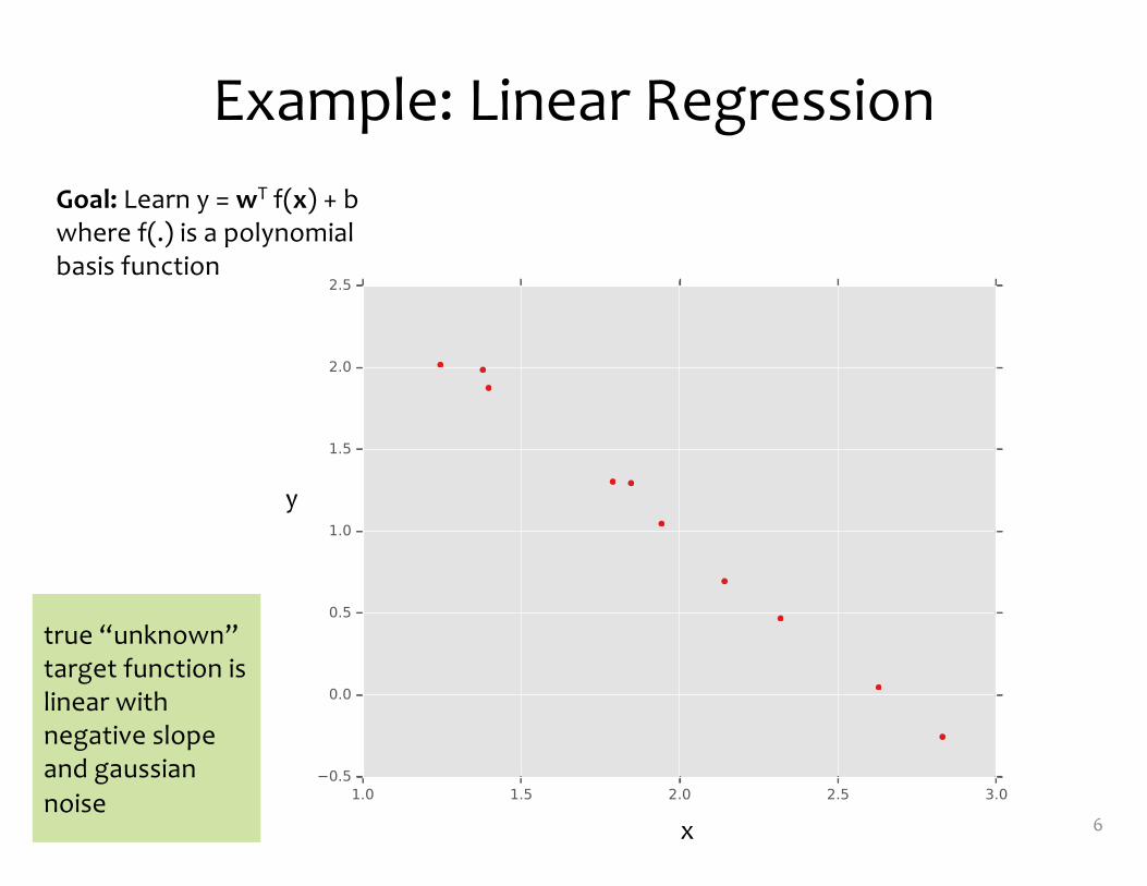
Example: Linear Regression
6x
y
Goal: Learn y = wT f(x) + bwhere f(.) is a polynomial basis function
true “unknown” target function is linear with negative slope and gaussiannoise

Example: Linear Regression
7x
y
Goal: Learn y = wT f(x) + bwhere f(.) is a polynomial basis function
true “unknown” target function is linear with negative slope and gaussiannoise

Example: Linear Regression
8x
y
Goal: Learn y = wT f(x) + bwhere f(.) is a polynomial basis function
true “unknown” target function is linear with negative slope and gaussiannoise
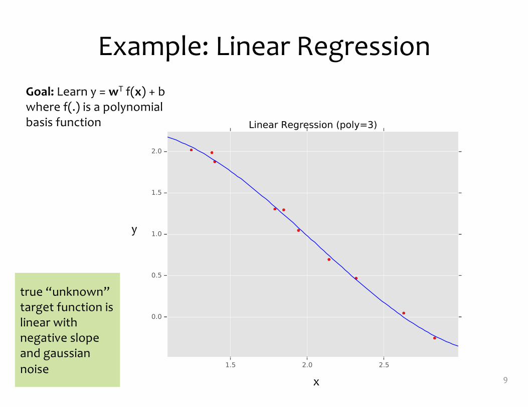
Example: Linear Regression
9x
y
Goal: Learn y = wT f(x) + bwhere f(.) is a polynomial basis function
true “unknown” target function is linear with negative slope and gaussiannoise

Example: Linear Regression
10x
y
Goal: Learn y = wT f(x) + bwhere f(.) is a polynomial basis function
true “unknown” target function is linear with negative slope and gaussiannoise

Example: Linear Regression
11x
y
Goal: Learn y = wT f(x) + bwhere f(.) is a polynomial basis function
true “unknown” target function is linear with negative slope and gaussiannoise
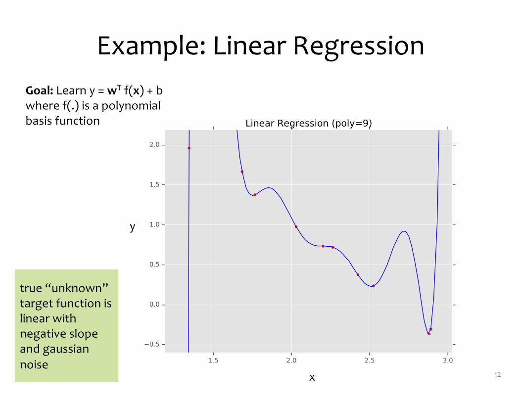
Example: Linear Regression
12x
y
Goal: Learn y = wT f(x) + bwhere f(.) is a polynomial basis function
true “unknown” target function is linear with negative slope and gaussiannoise
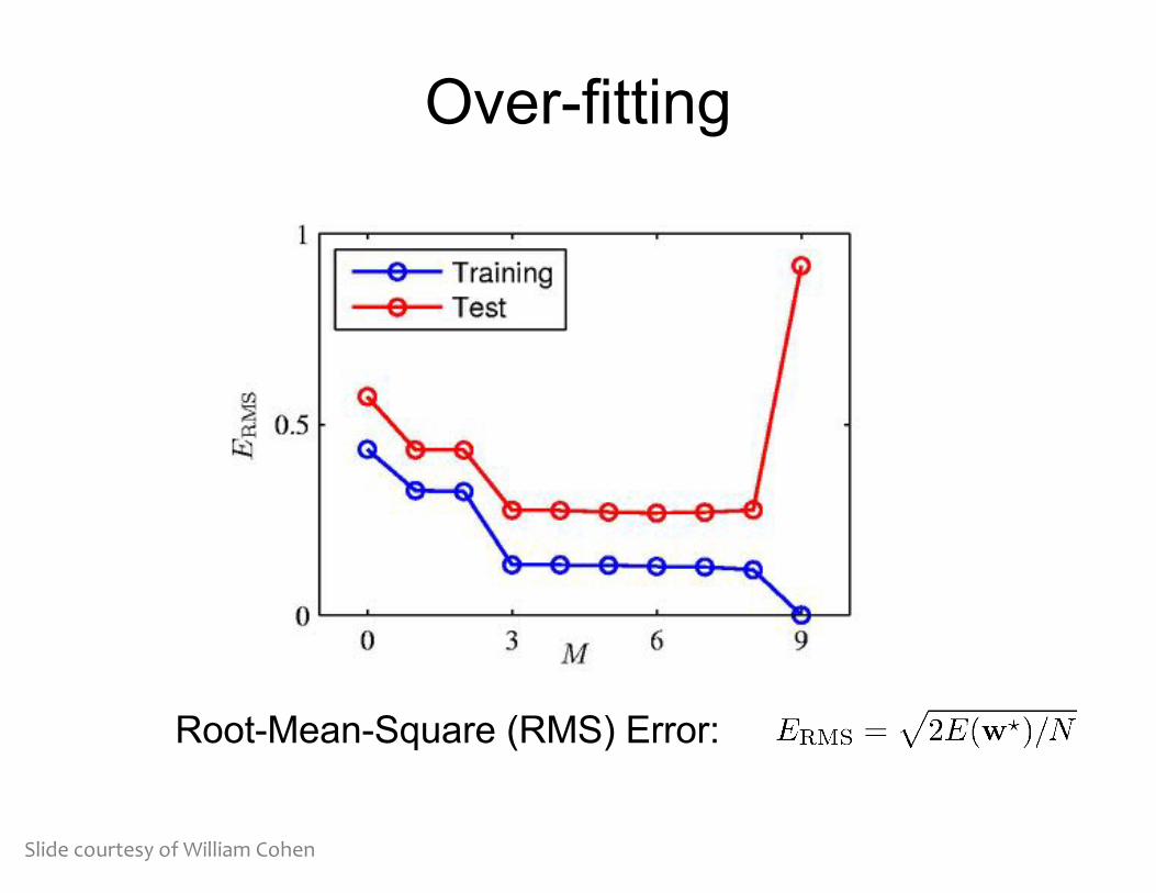
Over-fitting
Root-Mean-Square (RMS) Error:
Slide courtesy of William Cohen
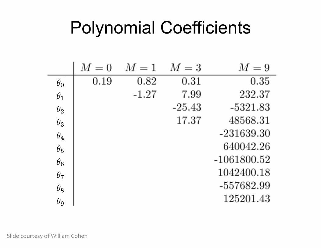
Polynomial Coefficients
Slide courtesy of William Cohen

Example: Linear Regression
15x
y
Goal: Learn y = wT f(x) + bwhere f(.) is a polynomial basis function
true “unknown” target function is linear with negative slope and gaussiannoise

Example: Linear Regression
16x
y
Goal: Learn y = wT f(x) + bwhere f(.) is a polynomial basis function
Same as before, but now with N = 100 points
true “unknown” target function is linear with negative slope and gaussiannoise

REGULARIZATION
17
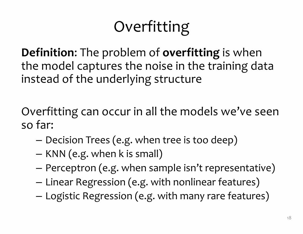
OverfittingDefinition: The problem of overfitting is when the model captures the noise in the training data instead of the underlying structure
Overfitting can occur in all the models we’ve seen so far: – Decision Trees (e.g. when tree is too deep)– KNN (e.g. when k is small)– Perceptron (e.g. when sample isn’t representative)– Linear Regression (e.g. with nonlinear features)– Logistic Regression (e.g. with many rare features)
18
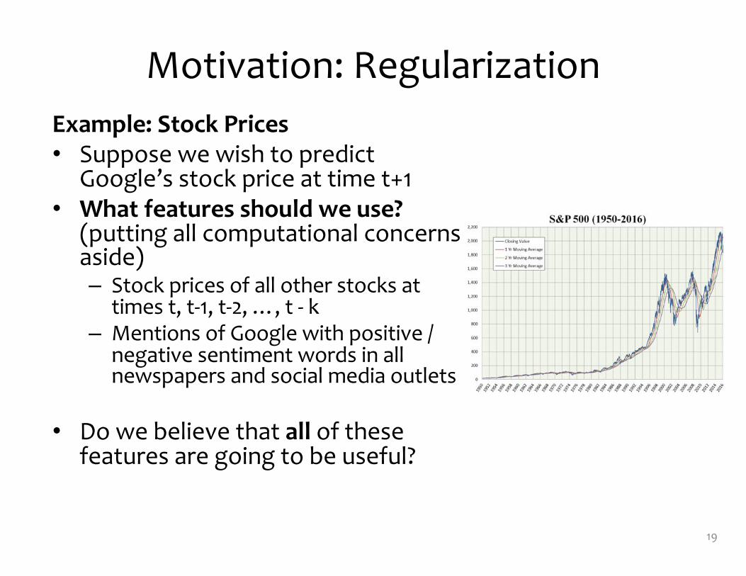
Motivation: RegularizationExample: Stock Prices• Suppose we wish to predict
Google’s stock price at time t+1 • What features should we use?
(putting all computational concerns aside)– Stock prices of all other stocks at
times t, t-1, t-2, …, t - k– Mentions of Google with positive /
negative sentiment words in all newspapers and social media outlets
• Do we believe that all of these features are going to be useful?
19

Motivation: Regularization
• Occam’s Razor: prefer the simplest hypothesis
• What does it mean for a hypothesis (or model) to be simple?1. small number of features (model selection)2. small number of “important” features
(shrinkage)
20

Regularization
Chalkboard– L2, L1, L0 Regularization– Example: Linear Regression
21

Regularization
22
Question:Suppose we are minimizing J’(θ) where
As λ increases, the minimum of J’(θ) will move…
A. …towards the midpoint between J’(θ) and r(θ)
B. …towards a theta vector of negative infinities
C. …towards a theta vector of positive infinities
D. …towards the minimum of J’(θ) E. …towards the minimum of r(θ)

Regularization ExerciseIn-class Exercise1. Plot train error vs. regularization weight (cartoon)2. Plot test error vs . regularization weight (cartoon)
24
erro
r
regularization weight

Regularization
25
Question:Suppose we are minimizing J’(θ) where
As we increase λ from 0, the the validation error will…
A. …increaseB. …decreaseC. …first increase, then decreaseD. …first decrease, then increaseE. …stay the same
Regularization
26
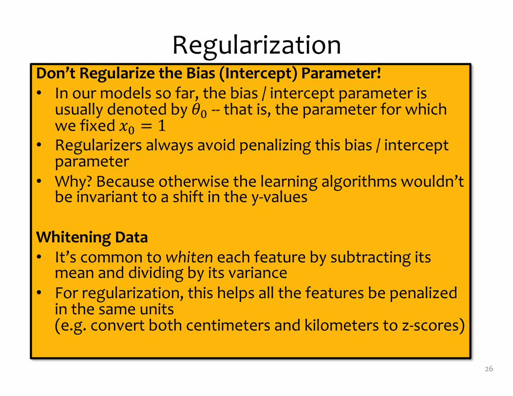
Don’t Regularize the Bias (Intercept) Parameter!• In our models so far, the bias / intercept parameter is
usually denoted by !" -- that is, the parameter for which we fixed #" = 1
• Regularizers always avoid penalizing this bias / intercept parameter
• Why? Because otherwise the learning algorithms wouldn’t be invariant to a shift in the y-values
Whitening Data• It’s common to whiten each feature by subtracting its
mean and dividing by its variance• For regularization, this helps all the features be penalized
in the same units (e.g. convert both centimeters and kilometers to z-scores)
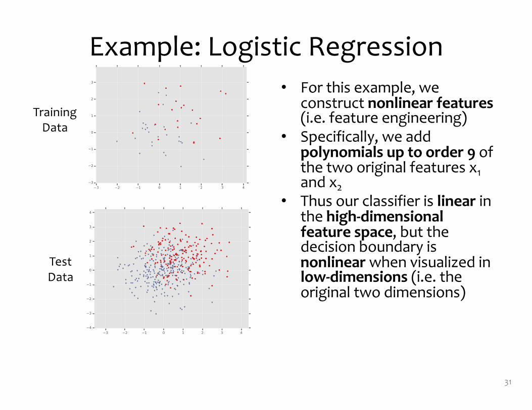
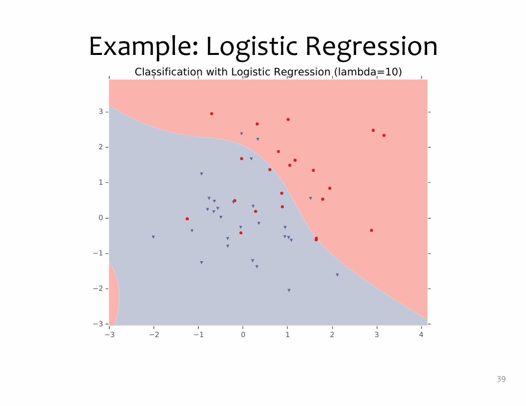
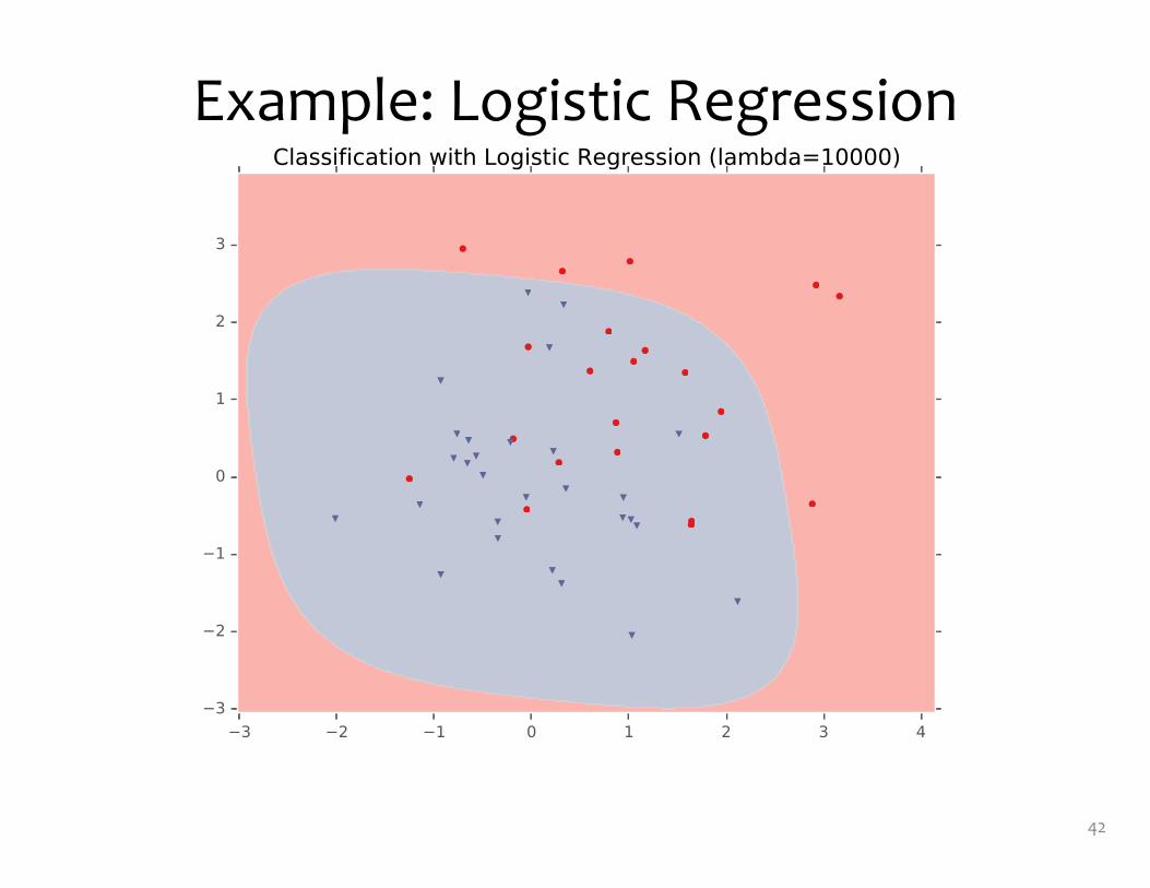
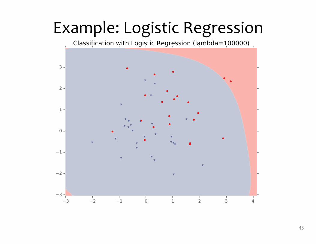
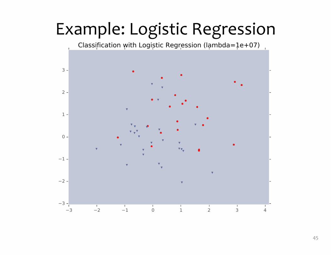
Example: Logistic Regression• For this example, we
construct nonlinear features (i.e. feature engineering)
• Specifically, we add polynomials up to order 9 of the two original features x1and x2
• Thus our classifier is linear in the high-dimensional feature space, but the decision boundary is nonlinear when visualized in low-dimensions (i.e. the original two dimensions)
31
Training Data
TestData
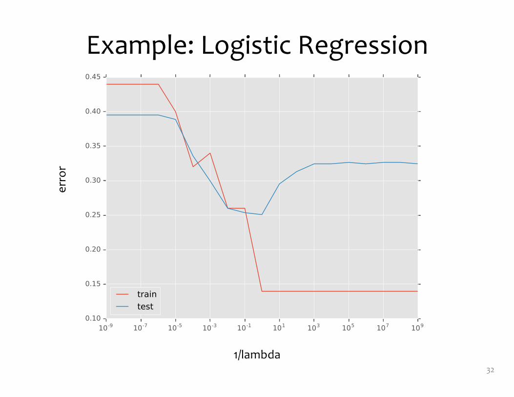
Example: Logistic Regression
32
1/lambda
erro
r

Example: Logistic Regression
33

Example: Logistic Regression
34

Example: Logistic Regression
35

Example: Logistic Regression
36
Example: Logistic Regression
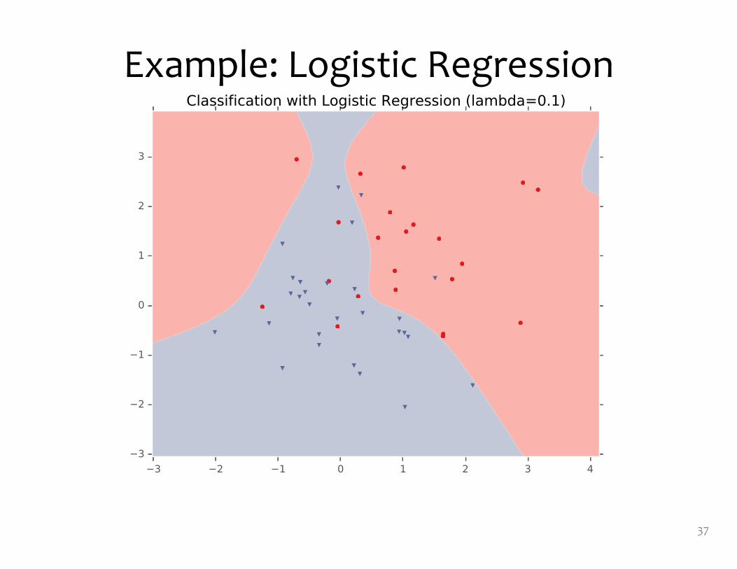
37
Example: Logistic Regression
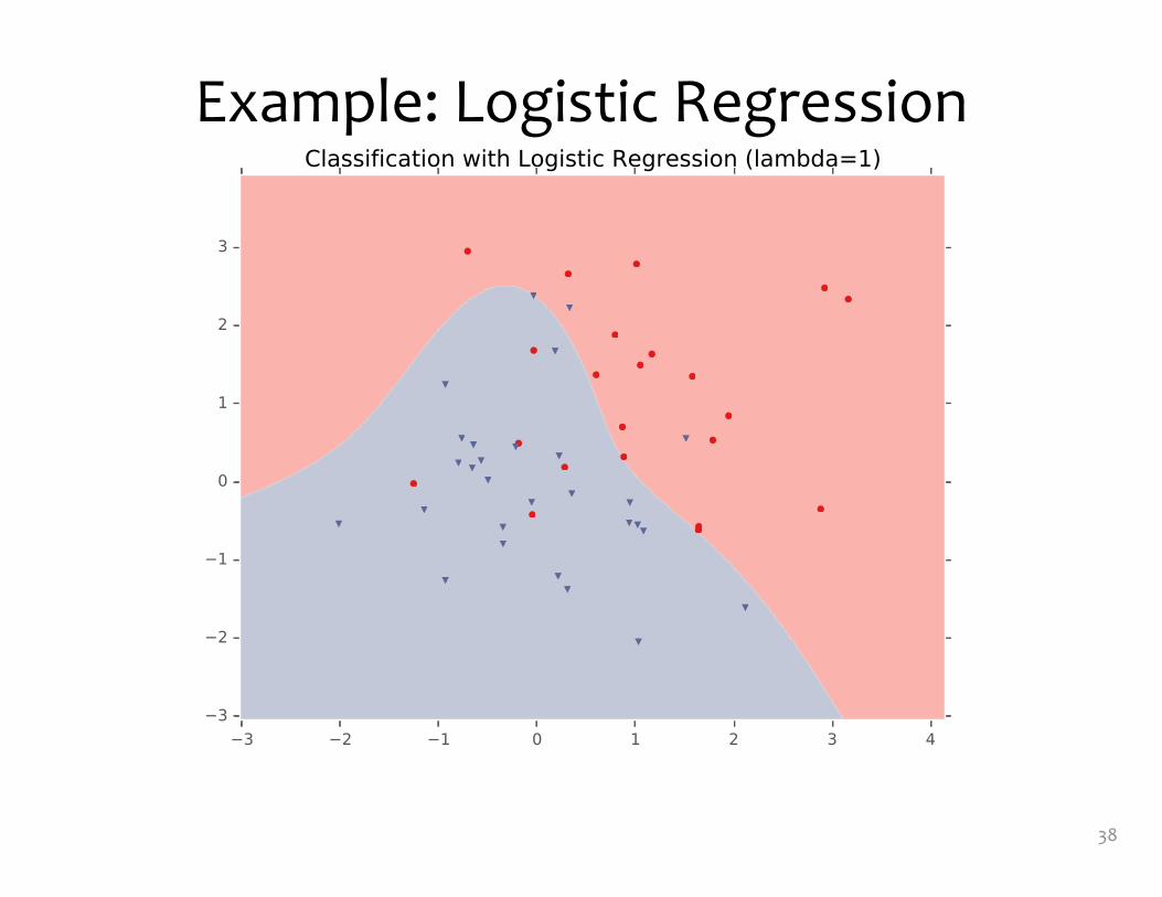
38
Example: Logistic Regression
39

Example: Logistic Regression
40

Example: Logistic Regression
41
Example: Logistic Regression
42
Example: Logistic Regression
43

Example: Logistic Regression
44
Example: Logistic Regression
45
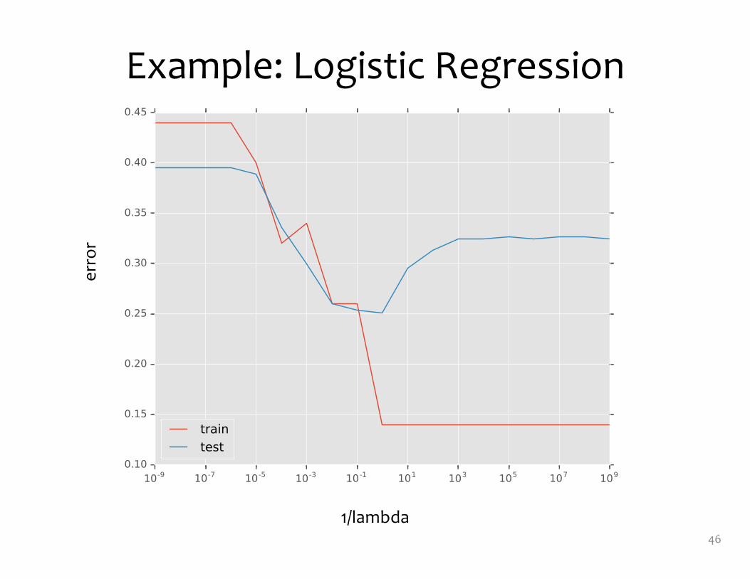
Example: Logistic Regression
46
1/lambda
erro
r

Regularization as MAP
• L1 and L2 regularization can be interpreted as maximum a-posteriori (MAP) estimation of the parameters
• To be discussed later in the course…
47

Takeaways
1. Nonlinear basis functions allow linear models (e.g. Linear Regression, Logistic Regression) to capture nonlinear aspects of the original input
2. Nonlinear features are require no changes to the model (i.e. just preprocessing)
3. Regularization helps to avoid overfitting4. Regularization and MAP estimation are
equivalent for appropriately chosen priors
49
Feature Engineering / Regularization Objectives
You should be able to…• Engineer appropriate features for a new task• Use feature selection techniques to identify and
remove irrelevant features• Identify when a model is overfitting• Add a regularizer to an existing objective in order to
combat overfitting• Explain why we should not regularize the bias term• Convert linearly inseparable dataset to a linearly
separable dataset in higher dimensions• Describe feature engineering in common application
areas
50

Neural Networks Outline
• Logistic Regression (Recap)– Data, Model, Learning, Prediction
• Neural Networks– A Recipe for Machine Learning– Visual Notation for Neural Networks– Example: Logistic Regression Output Surface– 2-Layer Neural Network– 3-Layer Neural Network
• Neural Net Architectures– Objective Functions– Activation Functions
• Backpropagation– Basic Chain Rule (of calculus)– Chain Rule for Arbitrary Computation Graph– Backpropagation Algorithm– Module-based Automatic Differentiation (Autodiff)
51

NEURAL NETWORKS
57

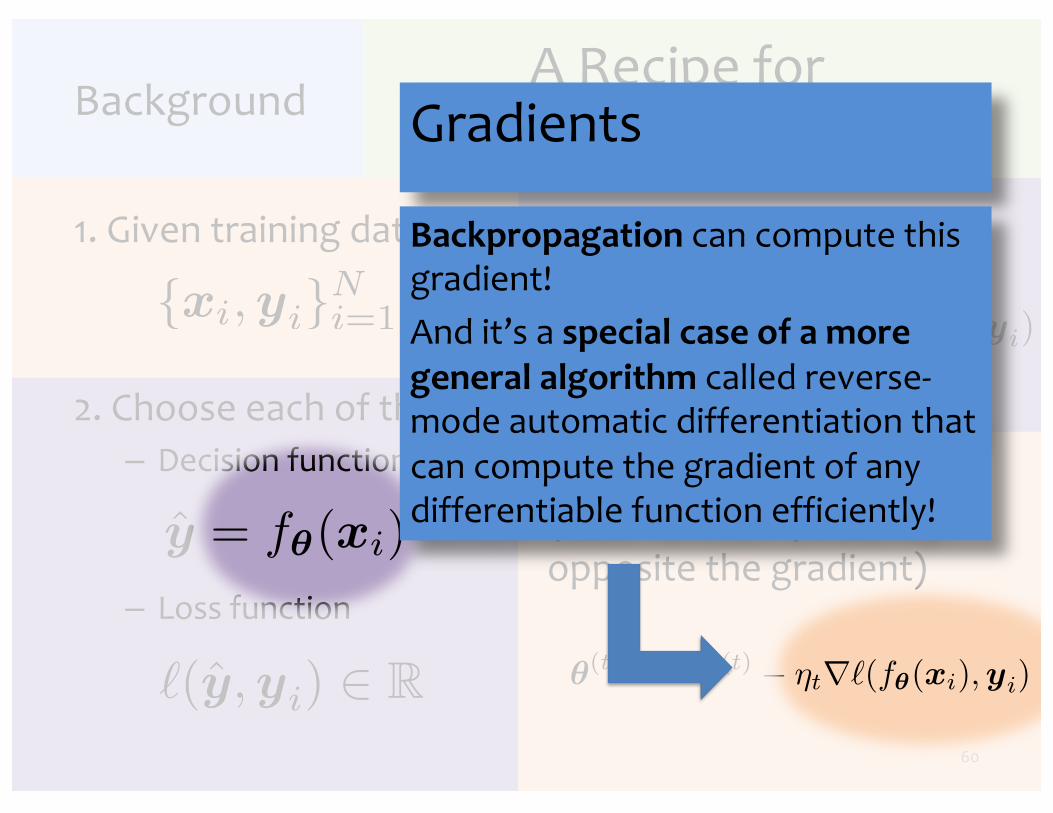
A Recipe for Machine Learning
1. Given training data:
58
Background
2. Choose each of these:– Decision function
– Loss function
Face Face Not a face
Examples: Linear regression, Logistic regression, Neural Network
Examples: Mean-squared error, Cross Entropy

A Recipe for Machine Learning
1. Given training data: 3. Define goal:
59
Background
2. Choose each of these:– Decision function
– Loss function
4. Train with SGD:
(take small steps opposite the gradient)
A Recipe for Machine Learning
1. Given training data: 3. Define goal:
60
Background
2. Choose each of these:– Decision function
– Loss function
4. Train with SGD:
(take small steps opposite the gradient)
Gradients
Backpropagation can compute this gradient!
And it’s a special case of a more general algorithm called reverse-mode automatic differentiation that can compute the gradient of any differentiable function efficiently!

A Recipe for Machine Learning
1. Given training data: 3. Define goal:
61
Background
2. Choose each of these:
– Decision function
– Loss function
4. Train with SGD:
(take small steps opposite the gradient)
Goals for Today’s Lecture
1. Explore a new class of decision functions (Neural Networks)
2. Consider variants of this recipe for training

Linear Regression
62
Decision Functions
…
Output
Input
θ1 θ2 θ3 θM
y = h�(x) = �(�T x)
where �(a) = a
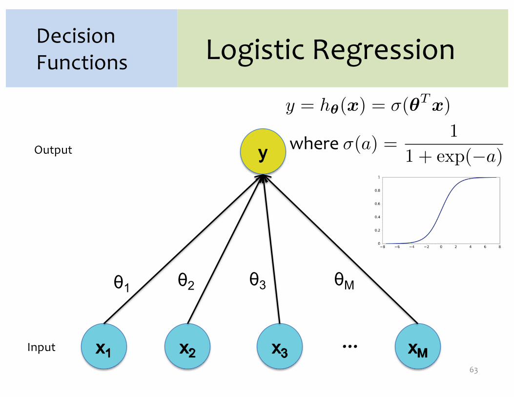
Logistic Regression
63
Decision Functions
…
Output
Input
θ1 θ2 θ3 θM
y = h�(x) = �(�T x)
where �(a) =1
1 + (�a)
y = h�(x) = �(�T x)
where �(a) =1
1 + (�a)
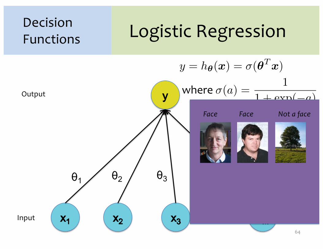
Logistic Regression
64
Decision Functions
…
Output
Input
θ1 θ2 θ3 θM
Face Face Not a face
y = h�(x) = �(�T x)
where �(a) =1
1 + (�a)
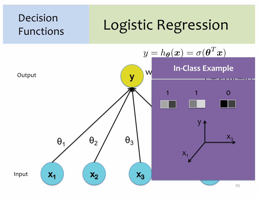
Logistic Regression
65
Decision Functions
…
Output
Input
θ1 θ2 θ3 θM
1 1 0
x1
x2
y
In-Class Example
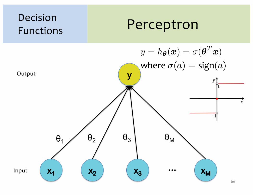
Perceptron
66
Decision Functions
…
Output
Input
θ1 θ2 θ3 θM
y = h�(x) = �(�T x)
where �(a) =1
1 + (�a)