Machine Learning & Data Mining CS/CNS/EE 155 Lecture 9: Decision Trees, Bagging & Random Forests 1.

1

Machine Learning & Data MiningCS/CNS/EE 155

Lecture 9:Decision Trees, Bagging &

Random Forests

2

Announcements

• Homework 2 harder than anticipated– Will not happen again– Lenient grading

• Homework 3 Released Tonight– Due 2 weeks later– (Much easier than HW2)

• Homework 1 will be graded soon.

3

Announcements

• Kaggle Mini-Project Released– https://kaggle.com/join/csee155 (also linked to from course website)– Dataset of Financial Reports to SEC– Predict if Financial Report was during Great Recession– Training set of ~5000, with ~500 features– Submit predictions on test set– Competition ends in ~3 weeks– Report due 2 days after competition ends– Grading: 80% on cross validation & model selection, 20% on accuracy– If you do everything properly, you should get at least 90%– Don’t panic! With proper planning, shouldn’t take that much time.– Recitation tomorrow (short Kaggle & Decision Tree Tutorial)

https://kaggle.com/join/csee155

https://kaggle.com/join/csee155

4

This Week

• Back to standard classification & regression– No more structured models

• Focus to achieve highest possible accuracy– Decision Trees– Bagging– Random Forests– Boosting– Ensemble Selection

5

Decision Trees

6

Person Age Male? Height > 55”

Alice 14 0 1

Bob 10 1 1

Carol 13 0 1

Dave 8 1 0

Erin 11 0 0

Frank 9 1 1

Gena 10 0 0

Male?

Age>8? Age>11?

1 0 1 0

Yes

Yes Yes No

No

No

x y

(Binary) Decision Tree

Don’t overthink this, it is literally what it looks like.

7

(Binary) Decision Tree

Male?

Age>8? Age>11?

1 0 1 0

Yes

Yes Yes No

No

No

Internal Nodes

Leaf Nodes

Root Node

Every internal node has a binary query function q(x).

Every leaf node has a prediction,e.g., 0 or 1.

Prediction starts at root node.Recursively calls query function.Positive response Left Child.Negative response Right Child.Repeat until Leaf Node.

AliceGender: FemaleAge: 14

Input:

Prediction: Height > 55”

8

Queries

• Decision Tree defined by Tree of Queries

• Binary query q(x) maps features to 0 or 1

• Basic form: q(x) = 1[xd > c]– 1[x3 > 5]– 1[x1 > 0]– 1[x55 > 1.2]

• Axis aligned partitioning of input space

10

Basic Decision Tree Function Class

• “Piece-wise Static” Function Class– All possible partitionings over feature space.– Each partition has a static prediction.

• Partitions axis-aligned– E.g., No Diagonals

• (Extensions next week)

11

Decision Trees vs Linear Models

• Decision Trees are NON-LINEAR Models!

• Example: No Linear Model Can Achieve 0 Error

Simple Decision TreeCan Achieve 0 Error

x1>0

1 x2>0

0 1

12


• Decision Trees are NON-LINEAR Models!

• Example: No Linear Model Can Achieve 0 Error

Simple Decision TreeCan Achieve 0 Error

x1>0

1 x1>1

1 0

13


• Decision Trees are AXIS-ALIGNED!– Cannot easily model diagonal boundaries

• Example: Simple Linear SVM can Easily Find Max Margin

Decision Trees RequireComplex Axis-Aligned Partitioning

Wasted Boundary

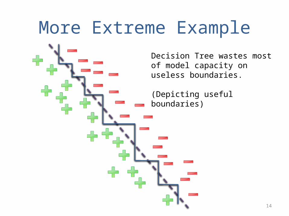
14

More Extreme ExampleDecision Tree wastes most of model capacity on useless boundaries.

(Depicting useful boundaries)

15


• Decision Trees are often more accurate!

• Non-linearity is often more important– Just use many axis-aligned boundaries to

approximate diagonal boundaries – (It’s OK to waste model capacity.)

• Catch: requires sufficient training data– Will become clear later in lecture

16

Real Decision Trees

Image Source: http://www.biomedcentral.com/1471-2105/10/116

Can get much larger!

17

Male?

Age>9? Age>11?

1 0 1 0

Yes

Yes Yes No

No

No

Decision Tree TrainingEvery node = partition/subset of SEvery Layer = complete partitioning of SChildren = complete partitioning of parent

Name Age Male? Height > 55”

Alice 14 0 1

Bob 10 1 1

Carol 13 0 1

Dave 8 1 0

Erin 11 0 0

Frank 9 1 1

Gena 10 0 0

S

x y

18

Thought Experiment

• What if just one node?– (I.e., just root node)– No queries– Single prediction for all data


Alice 14 0 1

Bob 10 1 1

Carol 13 0 1

Dave 8 1 0

Erin 11 0 0

Frank 9 1 1

Gena 10 0 0

S

x y

1

19

Simplest Decision Tree is just single Root Node(Also a Leaf Node)

Corresponds to Entire Training Set

Makes a Single Prediction: Majority class in training set

20

Thought Experiment Continued

• What if 2 Levels?– (I.e., root node + 2 children)– Single query (which one?)– 2 predictions – How many possible queries?


Alice 14 0 1

Bob 10 1 1

Carol 13 0 1

Dave 8 1 0

Erin 11 0 0

Frank 9 1 1

Gena 10 0 0

S

x y

Query?

? ?

Yes No

21

#Possible Queries = #Possible Splits=D*N

(D = #Features)(N = #training points)

How to choose “best” query?

22

Impurity

• Define impurity function:

– E.g., 0/1 Loss:

S

L(S) = 1 L(S1) = 0

S1 S2

L(S2) = 1

Impurity Reduction

= 0

Classification Errorof best single prediction

No Benefit FromThis Split!

23

Impurity


– E.g., 0/1 Loss:

S

L(S) = 1 L(S1) = 0

S1

S2

L(S2) = 1

Impurity Reduction

= 0


No Benefit FromThis Split!

24

Impurity


– E.g., 0/1 Loss:

S

L(S) = 1 L(S1) = 0

S1 S2

L(S2) = 0

Impurity Reduction

= 1


Choose Split withlargest impurityreduction!

25

Impurity = Loss Function

• Training Goal: – Find decision tree with low impurity.

• Impurity Over Leaf Nodes = Training Loss

S’ iterates over leaf nodesUnion of S’ = S (Leaf Nodes = partitioning of S)

Classification Error on S’

26

Problems with 0/1 Loss

• What split best reduces impurity?

S

L(S) = 1 L(S1) = 0

All Partitionings Give SameImpurity Reduction!

S1 S2 S1 S2

L(S2) = 1 L(S1) = 0 L(S2) = 1

27

Problems with 0/1 Loss

• 0/1 Loss is discontinuous

• A good partitioning may not improve 0/1 Loss…– E.g., leads to an accurate model with subsequent split…

S

L(S) = 1 L(S) = 1 L(S) = 0

S1 S2 S1 S2

S3

28

Surrogate Impurity Measures

• Want more continuous impurity measure

• First try: Bernoulli Variance:

pS’

L(S’

) P = 1/2, L(S’) = |S’|*1/4P = 1, L(S’) = |S’|*0P = 0, L(S’) = |S’|*0

Perfect Purity

Worst Purity

pS’ = fraction of S’ that are positive examples

Assuming |S’|=1

29

Bernoulli Variance as Impurity

• What split best reduces impurity?

S

L(S) = 5/6 L(S1) = 0

S1 S2 S1 S2

L(S2) = 1/2 L(S1) = 0 L(S2) = 3/4

Best!

pS’ = fraction of S’ that are positive examples

30

Interpretation of Bernoulli Variance

• Assume each partition = distribution over y– y is Bernoulli distributed with expected value pS’

– Goal: partitioning where each y has low varianceS

L(S) = 5/6 L(S1) = 0

S1 S2 S1 S2

L(S2) = 1/2 L(S1) = 0 L(S2) = 3/4

Best!

31

Other Impurity Measures

• Entropy:

– aka: Information Gain:

– (aka: Entropy Impurity Reduction)– Most popular.

• Gini Index:

See also: http://www.ise.bgu.ac.il/faculty/liorr/hbchap9.pdf(Terminology is slightly different.)

pS’

L(S’

)

Define: 0*log(0) = 0

pS’

L(S’

)Most Good Impurity Measures Look Qualitatively The Same!

32

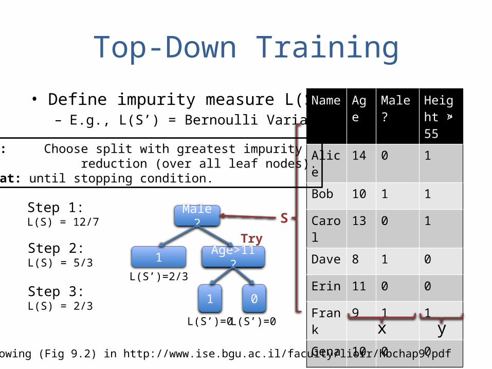
Top-Down Training

• Define impurity measure L(S’)– E.g., L(S’) = Bernoulli Variance


Alice 14 0 1

Bob 10 1 1

Carol 13 0 1

Dave 8 1 0

Erin 11 0 0

Frank 9 1 1

Gena 10 0 0

1 S

x y

Step 1:L(S) = 12/7

See TreeGrowing (Fig 9.2) in http://www.ise.bgu.ac.il/faculty/liorr/hbchap9.pdf

Loop: Choose split with greatest impurity reduction (over all leaf nodes).Repeat: until stopping condition.

33

Top-Down Training



Alice 14 0 1

Bob 10 1 1

Carol 13 0 1

Dave 8 1 0

Erin 11 0 0

Frank 9 1 1

Gena 10 0 0

Male? S

x y

Step 1:L(S) = 12/7



1 0

L(S’)=1

Step 2:L(S) = 5/3

L(S’)=2/3

34

Top-Down Training



Alice 14 0 1

Bob 10 1 1

Carol 13 0 1

Dave 8 1 0

Erin 11 0 0

Frank 9 1 1

Gena 10 0 0

Male? S

x y

Step 1:L(S) = 12/7



1 0Step 2:L(S) = 5/3

Step 3: Loop over all leaves, find best split.

L(S’)=2/3 L(S’)=1

35

Top-Down Training



Alice 14 0 1

Bob 10 1 1

Carol 13 0 1

Dave 8 1 0

Erin 11 0 0

Frank 9 1 1

Gena 10 0 0

Male? S

x y

Step 1:L(S) = 12/7



Age>8? 0Step 2:L(S) = 5/3

1 0Step 3:L(S) = 1

L(S’)=0

L(S’)=1

L(S’)=0

Try

36

Top-Down Training



Alice 14 0 1

Bob 10 1 1

Carol 13 0 1

Dave 8 1 0

Erin 11 0 0

Frank 9 1 1

Gena 10 0 0

Male? S

x y

Step 1:L(S) = 12/7



1 Age>11?Step 2:L(S) = 5/3

1 0Step 3:L(S) = 2/3

L(S’)=0 L(S’)=0

L(S’)=2/3

Try

37

Top-Down Training



Alice 14 0 1

Bob 10 1 1

Carol 13 0 1

Dave 8 1 0

Erin 11 0 0

Frank 9 1 1

Gena 10 0 0

Male? S

x y

Step 1:L(S) = 12/7



Age>8? Age>11?Step 2:L(S) = 5/3

1 0Step 3:L(S) = 2/3

L(S’)=0 L(S’)=0

1 0

L(S’)=0 L(S’)=0

Step 4:L(S) = 0

40

Properties of Top-Down Training

• Every intermediate step is a decision tree– You can stop any time and have a model

• Greedy algorithm– Doesn’t backtrack– Cannot reconsider different higher-level splits.

S S1 S2 S1 S2

S3

41

When to Stop?

• In kept going, can learn tree with zero training error. – But such tree is probably overfitting to training set.

• How to stop training tree earlier?– I.e., how to regularize?

Which one has better test error?

42

Stopping Conditions (Regularizers)

• Minimum Size: do not split if resulting children are smaller than a minimum size.– Most common stopping condition.

• Maximum Depth: do not split if the resulting children are beyond some maximum depth of tree.

• Maximum #Nodes: do not split if tree already has maximum number of allowable nodes.

• Minimum Reduction in Impurity: do not split if resulting children do not reduce impurity by at least δ%.

See also, Section 5 in: http://www.ise.bgu.ac.il/faculty/liorr/hbchap9.pdf

43

Pseudocode for Training


Stopping condition is minimum leaf node size: Nmin

Select from Q

44

Classification vs Regression

Classification Regression

Labels are {0,1} Labels are Real Valued

Predict Majority Class in Leaf Node

Predict Mean of Labels in Leaf Node

Piecewise Constant Function Class

Piecewise Constant Function Class

Goal: minimize 0/1 Loss Goal: minimize squared loss

Impurity based on fraction of positives vs negatives

Impurity = Squared Loss

45

Recap: Decision Tree Training

• Train Top-Down– Iteratively split existing leaf node into 2 leaf nodes

• Minimize Impurity (= Training Loss)– E.g., Entropy

• Until Stopping Condition (= Regularization)– E.g., Minimum Node Size

• Finding optimal tree is intractable– E.g., tree satisfying minimal leaf sizes with lowest impurity.

46

Recap: Decision Trees

• Piecewise Constant Model Class– Non-linear!– Axis-aligned partitions of feature space

• Train to minimize impurity of training data in leaf partitions– Top-Down Greedy Training

• Often more accurate than linear models– If enough training data

47

Bagging(Bootstrap Aggregation)

48

Outline

• Recap: Bias/Variance Tradeoff

• Bagging– Method for minimizing variance – Not specific to Decision Trees

• Random Forests– Extension of Bagging– Specific to Decision Trees

49

Outline

• Recap: Bias/Variance Tradeoff

• Bagging– Method for minimizing variance – Not specific to Decision Trees

• Random Forests– Extension of Bagging– Specific to Decision Trees

50

Test Error

• “True” distribution: P(x,y) – Unknown to us

• Train: hS(x) = y – Using training data: – Sampled from P(x,y)

• Test Error:

• Overfitting: Test Error >> Training Error

51


Alice 14 0 1

Bob 10 1 1

Carol 13 0 1

Dave 8 1 0

Erin 11 0 0

Frank 9 1 1

Gena 8 0 0


James 11 1 1

Jessica 14 0 1

Alice 14 0 1

Amy 12 0 1

Bob 10 1 1

Xavier 9 1 0

Cathy 9 0 1

Carol 13 0 1

Eugene 13 1 0

Rafael 12 1 1

Dave 8 1 0

Peter 9 1 0

Henry 13 1 0

Erin 11 0 0

Rose 7 0 0

Iain 8 1 1

Paulo 12 1 0

Margaret 10 0 1

Frank 9 1 1

Jill 13 0 0

Leon 10 1 0

Sarah 12 0 0

Gena 8 0 0

Patrick 5 1 1

…

L(h) = E(x,y)~P(x,y)[ L(h(x),y) ] Test Error:

h(x)y

Training Set STrue Distribution P(x,y)

52

Bias-Variance Decomposition

• For squared error:

“Average prediction on x”

Variance Term Bias Term

53

Example P(x,y)

x

y

54

hS(x) Linear

55

hS(x) Quadratic

56

hS(x) Cubic

57

Bias-Variance Trade-off

VarianceBias VarianceBias VarianceBias

58

Overfitting vs Underfitting

• High variance implies overfitting– Model class unstable– Variance increases with model complexity– Variance reduces with more training data.

• High bias implies underfitting– Even with no variance, model class has high error– Bias decreases with model complexity– Independent of training data size

60

Decision Trees are Low Bias, High Variance ModelsUnless you Regularize a lot…

…but then often worse than Linear Models

Highly Non-Linear, Can Easily Overfit

Different Training Samples Can Lead to Very Different Trees

61

Bagging

• Goal: reduce variance

• Ideal setting: many training sets S’– Train model using each S’– Average predictions

ES[(hS(x) - y)2] = ES[(Z-ž)2] + ž2

Variance BiasExpected ErrorOn single (x,y)

Z = hS(x) – y ž = ES[Z]

http://statistics.berkeley.edu/sites/default/files/tech-reports/421.pdf “Bagging Predictors” [Leo Breiman, 1994]

Variance reduces linearlyBias unchanged

sampled independently

S’P(x,y)

http://statistics.berkeley.edu/sites/default/files/tech-reports/421.pdf



62

Bagging

• Goal: reduce variance

• In practice: resample S’ with replacement– Train model using each S’– Average predictions

from S


Variance reduces sub-linearly(Because S’ are correlated)Bias often increases slightly

S’S

Bagging = Bootstrap Aggregation

“Bootstrapping”P(x,y)

ES[(hS(x) - y)2] = ES[(Z-ž)2] + ž2

Variance BiasExpected ErrorOn single (x,y)

Z = hS(x) – y ž = ES[Z]




63

Recap: Bagging for DTs

• Given: Training Set S

• Bagging: Generate Many Bootstrap Samples S’– Sampled with replacement from S• |S’| = |S|

– Train Minimally Regularized DT on S’• High Variance, Low Bias

• Final Predictor: Average of all DTs– Averaging reduces variance

64

“An Empirical Comparison of Voting Classification Algorithms: Bagging, Boosting, and Variants”Eric Bauer & Ron Kohavi, Machine Learning 36, 105–139 (1999) http://ai.stanford.edu/~ronnyk/vote.pdf

Variance

DT Bagged DT

Bett

er

Bias

65

Why Bagging Works

• Define Ideal Aggregation Predictor hA(x):– Each S’ drawn from true distribution P

• We will first compare the error of hA(x) vs hS(x)

• Then show how to adapt comparison to Bagging


Decision Tree Trained on S




66

Analysis of Ideal Aggregate Predictor

(Squared Loss)


Decision Tree Trained on S

Expected Loss of hS on single (x,y)

Linearity of Expectation

E[Z2] ≥ E[Z]2

( Z=hS’(x) )

Definition of hA

Loss of hA




67

Key Insight

• Ideal Aggregate Predictor Improves if:

• Bagging Predictor Improves if:


Large improvement if hS(x) is “unstable” (high variance)hA(x) is guranteed to be at least as good as hS(x).

Improves if hB(x) is much more stable than hS(x)hB(x) can sometimes be more unstable than hS(x)

Bias of hB(x) can be worse than hS(x).




68

Random Forests

Random Forests

• Goal: reduce variance– Bagging can only do so much– Resampling training data asymptotes

• Random Forests: sample data & features!– Sample S’ – Train DT• At each node, sample features

– Average predictions

“Random Forests – Random Features” [Leo Breiman, 1997]http://oz.berkeley.edu/~breiman/random-forests.pdf

Further de-correlates trees

http://oz.berkeley.edu/~breiman/random-forests.pdf


70

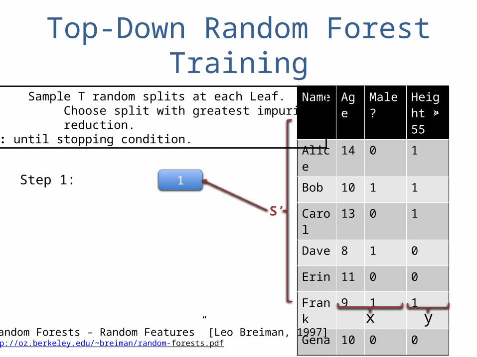
Top-Down Random Forest TrainingName Age Male? Height

> 55”

Alice 14 0 1

Bob 10 1 1

Carol 13 0 1

Dave 8 1 0

Erin 11 0 0

Frank 9 1 1

Gena 10 0 0

1

S’

x y

Loop: Sample T random splits at each Leaf. Choose split with greatest impurity reduction.Repeat: until stopping condition.

Step 1:




71


> 55”

Alice 14 0 1

Bob 10 1 1

Carol 13 0 1

Dave 8 1 0

Erin 11 0 0

Frank 9 1 1

Gena 10 0 0

Age>9?

S’

x y

Step 1:


1 0Step 2:

Randomly decide only look at age,Not gender.


1



72


> 55”

Alice 14 0 1

Bob 10 1 1

Carol 13 0 1

Dave 8 1 0

Erin 11 0 0

Frank 9 1 1

Gena 10 0 0

Age>9?

S’

x y

Step 1:


Male? 0Step 2:


Randomly decide only look at gender.

1 1Step 3:

Try



73


> 55”

Alice 14 0 1

Bob 10 1 1

Carol 13 0 1

Dave 8 1 0

Erin 11 0 0

Frank 9 1 1

Gena 10 0 0

Age>9?

S’

x y

Step 1:


1 Age>8?Step 2:


Randomly decide only look at age.

01Step 3:

Try



74

Recap: Random Forests

• Extension of Bagging to sampling Features

• Generate Bootstrap S’ from S– Train DT Top-Down on S’– Each node, sample subset of features for splitting• Can also sample a subset of splits as well

• Average Predictions of all DTs




Better

Average performance over many datasetsRandom Forests perform the best

“An Empirical Evaluation of Supervised Learning in High Dimensions”Caruana, Karampatziakis & Yessenalina, ICML 2008

Random Forests

76

Next Lecture

• Boosting– Method for reducing bias

• Ensemble Selection– Very general method for combining classifiers – Multiple-time winner of ML competitions

• Recitation Tomorrow:– Brief Tutorial of Kaggle– Brief Tutorial of Decision Tree Scikit-Learn Package

• Although many decision tree packages available online.

Machine Learning & Data Mining CS/CNS/EE 155 Lecture 9: Decision Trees, Bagging & Random Forests 1.

Documents

Transcript of Machine Learning & Data Mining CS/CNS/EE 155 Lecture 9: Decision Trees, Bagging & Random Forests 1.