IEEE TRANSACTIONS ON AUTOMATIC CONTROL, VOL. 40. NO. 7. JULY 1995 1199

Machine Learning and Nonparametric Bandit Theory Tze-bung Lai and Sidney Yakowitz, Member, IEEE

Abstruct-In its most basic form, bandit theory is concerned with the design problem of sequentially choosing members Rom a given collection of random varisbk 80 ulat the regret, i.e.,

increasing n. Here p, is the expected value of the bandit arm (i.e., random vrrrlable) indexed by j , T, ( j ) is the number of times arm jhasbeenselecteainthefirstndeeiskxrstqges,amlp* = sup,p,. The present paper coatribotes to the theory by considering the situation in wbich observations are dependent. To begin with, the dependency is presumed to depend only on past observations of the same ann, but Mer, we allow that it may be with respect to the entire past pml that the set of a r m is infinite. This brings queues nod, more generally, controlled Markov proasses into our ~ U F V ~ W . Thus OUT “black-box” methodology is sultable for the case when the o d y observables are cast values and, in particulpr, the probability structure and 1- function are unknown to the desigaer. The conelbn of the aaalysis is that under lenient conditions, using dgorithms prescribed herein, risk growtb hi conrmensurate with that in the simplest i.i.d. cases. Our methods repreaent an alternative to receat stochastic- approximatbdperturhtion-analysis iderrs for tuning queues.

R, = C,(/L* - p , )ET, ( j ) , grows ~8 lowly 98 p ~ ~ ~ i b l e with

I. INTRODUCTION

ANDIT theory, with origins and motivation in sequential B testing of medical treatments, deals, in the simplest case, with the challenge of choosing between the arms of a two- armed slot machine. At each “pull of an arm,” the user receives a reward chosen by a (hypothetically) random mechanism. The outcomes associated with a sequence of choices of a given arm are traditionally taken to be independent and identically distributed (i.i.d.) and to belong to a known parametric family, usually Bernoulli. Naturally, the goal is to select the arm for which the expected reward is highest. One must experiment to see which arm that is. The appellation “bandit” stems from recognition that the expected reward is universally lower than the fee for pulling the arm.

Much of the literature of bandit theory is set in a Bayesian context, and as one can see by reading [l] or [2], even in elementary cases, Bayesian strategies typically require excru- ciating calculations.

The foundation of the present study is due, in large part, to the pioneering work of Robbins [3] which is nonparametric and non-Bayesian. A certainty-equivalence rule with forcing was introduced in [3] and Was shown to have the property

Manuscript received May 9, 1994; revised December 9, 1994. Recom- mended by Associate Editor, P. Nab. This work was supported in part by National Science Foundation Grants DMS-9104432, INT-9201430, and ECS- 891362, National Security Agency Grant MDA90992-H-3092, and National Institutes of Health Grant A37535-01.

T.-Z. Lai is with the Department of Statistics, Stanford University, Stanford, CA 94305 USA. S. Yakowitz is with the Systems and Industrial Engineering Department,

University of Arizona, Tucson, Ai! 85721 USA. IEEE Log Number 941 1879.

.

that asymptotically the relative number of times the best arm is chosen converges a.s. to one, assuming only independence and finite first moments.

The present work follows Robbins’ nonpyametrichon- Bayesian formulation, but drops the independence assumption. It employs concepts established in the i.i.d. analysis by Lai and Robbins [4], who proposed a strategy for IC-armed parametric bandits which achieves a regret growth, with number n of decision epochs, of

(1.1)

Furthermore, they established that growth rate (1.1) is a lower bound for any strategy for which the regret is of order o(na), any a > 0, uniformly over all parameters. That is, the regret rate in (1.1) cannot be improved, even by Bayesian strategies, even for a two-armed Bernoulli bandit, and even if the probability of one of the arms is specified. Thus it may be surprising that in Section 11, we show that without making parametric assumptions we can still achieve O(1ogn) growth in regret under reasonably inclusive conditions.

Mallows and Robbins [5] were the first to consider the case of a countably infinite number of arms and generalized Robbins’ [3] forcing schemes to attain a regret growth of o(n). In this case, the constant ck in (1.1) typically goes to infinity as k increases, implying that the regret of any uniformly good procedure is of larger older than logn. In Section 111, however, we give a procedure which improves on the Mallows-Robbins result by assuring regret growth of the order O(an log T I ) for any specified nondecreasing sequence a, -+ 00, the domain of bandit problems still including a large class of unbounded dependent variables. These results generalize and improve upon a nonparametric bandit study of Yakowitz and Lowe [6] .

The culmination of the present study is an extension to adaptive learning ana control in Markov decision processes. Agrawal er al. [7] studied the parametric case of fipite state space and finite set of stationary control laws and obtained a lower bound for the regret Rn,z of uniformly good rules

(1.2)

for any initial state 2. Graves and Lai [8] showed that (1.2) holds in general state spaces and derived a general constant C. Making use of sequential tegting theory, they introduced uncertainty adjustments into the certainty-equivalence rule to attain lower bound (1.2). In Section IV, we first extend our nonparametric approach to the case of infinitely (but countably) many stationary conttol laws for Markov decision processes with general state spaces and still achieve a regret growth of an log n for any given sequence a, --t 00, however

(ck + o( 1)) log

*

Rn,z 2 (C + o( 1)) log

0018-9286/95$04.00 0 1995 IEEE

I200 El33 TRANSACTIONS ON AUTOMATIC CONTROL, VOL. 40, NO. 7, JULY 1995

slowly. The final theoretical development, also in Section IV, allows the space of stationary control laws to be nondenumer- able. The central result is a sampling strategy assuring that, under given conditions, the “learning loss” has a growth rate of O(a, log2 n) for any given monotonic unbounded sequence {a,,}. This improves upon a result of Yakowitz et al. [9].

It is our earnest hope that the strategies offered here are of practical as well as theoretical interest. Section V ex- plores applications to tuning a queue with unknown statistical properties. In view of our theory, the usual assumptions regarding exponential distribution of arrivals and services are dispensed with, and yet empirically, we see average perfor- mance approach optimality, in accordance with the theory. Our results illustrate the usefulness of a black-box approach to stochastic optimization, with which one can deal with certain processes having nonlinear dynamics and unknown structure and still have long-run average cost optimality and regret rates comparable to the optimal rates for linear control and prediction problems established by Lai and Ying [lo].

11. A NONPARAMETRIC APPROACH TO THE MULTIARMED BANDIT PROBLEM WITH DEPENDENT OUTCOMES

Imagine that there are k stochastic sequences X, = {Xt(’), t 2 l}, for j = l , . . . , IC, such that EIXf)) < 00 and lim,,,n-lES$) = p, exists and is finite. Here, Si’’ = xi’) + . . . + x?). In this section, we relate a sequential sampling strategy for choosing among these processes so that the regret

is of the order O(logn) as n -+ 00. The notation above is that T,(j) is the number of observations from X, that have beenmadeuptostagen,andp* = m a x { p , , j = l , . . . k } . A sampling strategy is a data-driven function; the selection of X, at time n depends entirely on the observed rocess/outcome

the outcome if j ( t ) is the process index chosen at time t. Intuitively, when an arm is chosen, the process associated with that arm takes up where it left off last time it was called, even if there had been intervening calls to other arms. This is in contrast to controlled Markov processes, to which attention turns in Section IV.

In this study, no parametric assumptions about the distri- bution of the stochastic seqpences X, are adopted, and our nonparametric policies do not involve modeling the dynamics and the distributions of the X p ) ’ s . Moreover, we will not require X?), X t ) , . . . to be i.i.d. for fixed j , as in [6] nor to be functions of geometrically ergodic Markov chains, as postulated in [ll]. In fact, the X, sequence need not even be stationary. Defining the optimal index set L = { j : p, = p * } , we shall only assume polynomial bounds on the tails of the distributions of Si’) for every j E { 1, . + . , k} and certain exponential bounds on the left tails of the distributions of Si’) for j E L. Specifically, we assume the following:

pairs ( j ( t ) , y t ) , t < n, where gt = XTt(3(t)) &)) represents

Al) There exist y > 0 and 0 < v < p* - maxigL pi such that

maxP[m-’S$) - p* < -171 = O(e-Tm). ,EL

A2) There exists c > 0 such that Tn

A3) For every E > 0

mgxP[Im-’S$) - pjl > E ] = ~ ( m - ~ ) . 3

Remarks: 1) Suppose that the Xy) are independent random variables

with

maxsupE[exp(80(EX,(3) - X p ) ) ) ] < 00 t2l

for some 80 > 0. Then for 0 5 6 < Be, since eer - 1 - 19z 5 !j62{~21{,50) + (0, - 8)-2eeOzI{z>o,} (noting that (60 - 19)2z2eBr 5 ee@ if s > 0), it follows that

E[exp(e(Ex,(3) - xf)))] - 1 5 o2 x {Var(Xt(’)) + (80 -

E[exp(Bo(EX,(3) - X,‘”))]}.

Therefore given any A > 0, there exists 8 > 0 such that

From the Markov inequalities, it then follows that Al)-A3) hold with A < 77 < p* - max,6Lpz and y = 8(77 - A) in Al) and with c in A2) large enough so that O(c - A > 1, since the moment generating

generating functions of E(x,(~)) - x ~ ) ( I 5 t 5 m) and since

function of E(Sm 2 ) ) - Sk) is the product of the moment

m

E ( @ - = E ( X p - t=l

+ 6 Var(Xt(3))

. Var(X2)) = 0 ( m 2 ) .

l<s< t<m

More generally, instead of independence, we can assume that {x,’“ - p,,t 2 1) is a martingale difference sequence with respect to an increasing sequence of 0- fields {Fp), t 2 1) such that

for some 8 > 0 and 0 < A < p* - maxigLpi. Then Al)-A3) again hold with the above choices of v , ~ , and

LA1 AND YAKOWITZ: NONPARAMETRIC BANDIT THEORY

If X,(3) = g(2,(3)), where 2:) is a uniformly recurrent Markov chain, or more generally, if Xp) is the additive component of a uniformly recurrent Markov additive process, such that E,exp(BX,(J)) < 00 for some 6 and reference measure v, then A l t A 3 ) follow from large deviation results analogous to those for sums of i.i.d. random variables (cf. [12]). Other examples of X p ) satisfying Al)-A3) include multiplicative sequences and generalized Gaussian se- quences (cf. [ 13]), hypermixing processes (cf. [ 14]), and bounded strong (or uniform) mixing sequences with fast enough decay for the mixing rates (cf. [151-[17]).

The basic idea of the sampling rule explored here is to replace the parametric likelihood-based testing strategies of Lai and Robbins [4] by non arametric sample-mean-based

q > 0. To begin with, at stage j = 1, . . . , k, the rule takes one observation from X,. Now suppose that n 2 k observations have been taken. Since T,( 1) + . . + T,(k) = n, we can choose j , E { l , . . . , k } such that

analogs. Let X t ( j ) = t-lStJ). P Take 0 < S < l / k and

X T n ( ~ , l ) ( j n ) = ma{xTn(~)(.j):Tn(j) 2 Sn}.

At stage n + 1, if n + 1 = j(mod k) with 1 5 j 5 k, we take an observation from X, only if

(2.1) X%(Jn)( jn) 5 x T n ( J ) ( 3 ) + %,Tn(J)

and sample from XJn, otherwise, where

u, ,~ = A,(logn)/t, for 1 5 t < logn, = A,, for logn 5 t < A,logn, = 0, for t 2 A, logn (2.2)

and A, will be specified in Theorem 1 below. This sampling rule will be denoted by q5*. The effect of condition (2.1) is to assure that the apparently-inferior arms are chosen often enough to eventually detect whether they are actually the best. Thus, by (2.1), arms with lower means are chosen if either the sample averages are sufficiently close to the leading arm or if too few observations have been made of this arm.

Theorem 1: i) Suppose that an upper bound A 2 max{l,y-’,c} for

the y and c in Al) and AS) is known and suppose that the A, in (2.2) is chosen to be A for all n. Then the regret R, of the rule q5* satisfies R, = O(1ogn).

ii) Without assuming prior knowledge of an upper bound for y-’ and c , let A, be any nondecreasing sequence of positive numbers such that limn+m A, = 00. Then R, = O ( A , log n) for the rule qY.

Proofi To prove i) we shall first show that

n

t=l

= O(1ogn) for any j # L and y > p j . (2.4)

1201

To prove (2.3), first apply Al) to conclude that

P b * - r l > X t ( j ) }

= O(exp(-logn)) = ~ ( n - l ) . t2.y-1 log n

By (2.2), A2) and recalling that A 2 max{c,y-l, 1)

5 ma P{p*t > Sf) + Alogn} I E L t<logn

= O(exp(- logn)).

Let b = (A + q ) / c ( > 1). For v = 0,1, and b” logn 5 t 5 bV+l log n, we have (A + q)t 2 cbVs1 logn, and therefore by (2.2) and A2), if b”+l I A

P{p*t > Si’’ + ( A + q)t} bV log n<t<b”+’ log n,

Lmax c P{ sp - p* t < -cbVS1 log n } t i bY+‘ log n ,

I E L

= O(exp( - log n)) .

Combining the above bounds yields (2.3).

for t 2 Alogn To prove (2.4), take j # L and 9 > pj . Since a,,t = 0

by A3). Since C t s 4 1 0 g n P [ X t ( j ) + an,t 2: Y] I (2.4) follows.

The rest of the proof of i) is similar to that of Theorem 34) of Lai and Robbins [4]. Note in this connection that (2.3) and (2.4) are analogous to (3.1) and (3.2) of [4]; moreover, by A3)

which is analogous to (3.5) of [4]. To prove ii), note that (2.3) still holds, since A, > max{ 1:

y-l , c) for all large n; moreover, (2.6) still holds. We replace (2.4) by

t= l

= O(A, log n) for any j $? L and y 2 pj

which can be proved by replacing A log n in (2.5) by A, log n. The rest of the proof is again similar to that of Theorem 3-i) of [4]. 0

1202 IEEE TRANSACTIONS ON AUTOMATIC CONTROL, VOL. 40, NO. 7, JULY 1995

III. GENERALIZATION TO THE CASE OF INEWITELY MANY A R M S

We now expand the setting of Section II by supposing that there are countably infinitely many stochastic sequences Xj such that the pLJ have a finite maximum ,U*, with L := {j: pJ = p* ) # 8 and p* > supjILpj. Assumptions Al)-A3) in Section I1 have been stated in a form that can be adapted without any change, other than the substitution of “sup” for “ma,” in the present case of infinitely many bandit processes.

Let IC, be a sequence of positive integers such that

I C , 2 k n - l . ICn + 00 but I C , = 0(na) as n --+ 00, for every a > 0. (3.1)

+ P { W ) 2 p* - 77) 7 by (2.2) 1 t2An logn

kn

5 [An l ogn + 0(1)] C(P* - p j ) , by A3). (3.6) j=1

Making use of (3.4)-(3.6), we can modify the proof of Lemma 1 and Theorem 34) of Lai and Robbins [4] to complete the proof. 0

Suppose that supj lpfI < 30. Then Cj<kn(p* - p j ) = 0 (k,). Therefore by Theorem 2, if we choose k, = O ( 6 ) and A, = O(an/kn) in the rule 6, then 6 has regret R, = O(a , logn) .

Define X o ( j ) = 0 and -gt(j) = t-’SP) for t 2 1. At stage n + 1, if n + 1 E j(mod IC,) with j E (1,. a kn}, we take an observation from X j only if

N. NONPAMMETRIC LEARNING ALGORITHMS FOR CONTROLLED MARKOV CHAINS

(3.2) A. Countable Set of Stationary Control Laws X*,,(j,,)(jn) I X ~ ~ ( j ) ( j ) + an,Tn(j) and sample from X,,, otherwise, where a,,t is defined by (2.2) for and we set a,,o = 30, and j , E {l,. . . , is so chosen that

Consider a stochastic system described by a Markov chain on state space X, with control set U, transition probability function {Pu(z,B) : z E X , B E B,u E U}, where L3 is a a-field of subsets of X. Let r ( X t , U,) represent

I -

XT,, ( 3 % ) (.in) the one-step reward at time t. For a stationary control law n

= m a x { X ~ ~ ( ~ ) ( j ) : 1 5 j 5 I C , and Tn(j) 2 -}. 2kn

(3.3)

The sampling rule, which will be denoted by 6, is a natural extension of the rule qY in Section U, replacing the fixed set of k arms by a slowly increasing set with cardinality k, -+ 30.

Theorem 2: Let a, be any nondecreasing sequence of positive numbers such that a, + 30 and azn = O_(an) as n .+ 00. Suppose that the A, and k, in the rule 4 are so chosenthat (3.1) holds, A, .+ 30 but IC:+A, C j g k n ( p * - p j ) = O(a,). Then the regret R, of the rule 6 satisfies R, = 0

Proof: Replacing IC in the proof of Theorem 1 by IC,, (an logn) .

we have

(3.4)

= 0 I C , t - 2 ) = o(n- lk i ) (3.5)

in place of (2.3) and (2.6). Recall that 0 < 77 < p* -supjcL p j in Al). Instead of (2.4) we now use

( n / 2 k n < t < n

n

g: X -, U, we shall use Pg to denote the transition probability function { P g ( Z ) ( z , B ) : z E X , B E B } of the controlled Markov chain under the control law g and P i to denote the conditional probability measure of this chain starting at state z. Let 9 be a countable (possibly infinite) set of stationary control laws such that

n

exists for every g E 9 and z E X, &d there is a maximum value A * of Xg over 9. For a control rule #J that chooses adaptively some stationary control law in 9 to use at every state, its regret is defined by

Rn,z = C(X* - Xg)EeTn(g) SEG

where T,(g) is the number of times that the control rule q5 uses the stationary control law g up to stage n and E, denotes expectation under the probability measure P, of the controlled Markov chain starting at z and using control rule 4. Similar to the sequential strategy of bandits in Section 11, #J chooses a control law #Jn E 9 at epoch n on the basis of the history of controlloutcome pairs (#Jt,Xt), t < n. But a bothersome difference is that for controlled Markov chains, Xt is not governed by the Markov state from the last time the same control as $t was called, but rather by the immediately preceding state X t - l , regardless of whether or not 4, = &I. Thus the observed performance of the law +t is skewed by starting from a “transient condition” every time the stationary control is switched.

We shall let z- denote the negative part of a real number z , i.e., z- = IzI if z < 0 and z- = 0 otherwise. We shall also denote the largest integer I z by [ z ] .

LAI AND YAKOWITZ: NONPARAMETRIC BANDIT THEORY 1203

Assumptions: Let L = {g E 9: A, = A'}. Assume that L

C1) suPzEx,gEG In-'EZ(C;=i r(Xa,g(Xa)>> - AgI + 0

C2) SUPzEX,g€g,t21 ~,SIr(Xt,g(Xt)) - E,Sr(Xt,g(Xt))14

C3) sUPzEX,gEL,t>l E,S[exP(e{E,ST(X,,g(Xt)) - r ( X t , 9

is not empty and that A' > supgeL A, and the following:

a s n - + 0 0 ,

< m,

(Xt))})] < 00 for some 6 > 0. Condition C1) requires that the convergence in (4.1) holds

uniformly in z E X and g E 8. The combination of C1) and C2) is related to Condition A3) in the bandit theory of Section II; see Remark 1. Likewise the combination of C1) and C3) is related to Conditions Al) and A2) and gives exponential bounds for the left tails of the distribution of

r(X,,g(XI)) under Pg; moreover, as in Al) and A2), we only require C3) to hold for g E L (the set of best controls).

Let S = (91, g2, . .}. Our learning strategy is based on the following modification of the procedure in Section III: Instead of switching between stationary control laws from one stage to another, we shall adhere to the same g for a consecutive block of stages, with the block size growing with n. This is needed because in the controlled Markov process, when the control law g is changed, the transition probability function Pg is also changed. Accordingly we adopt the following scheme. Take c > 1 and let ni = [c']. Partition {n, ,n2,+1, . - . ,n ,+1 -1) intom(i) := [(n,+l-n,)/i] blocks of consecutive integers, each block having length i except possibly the last one whose length may range from i to 2i - 1. Label these blocks as Bi, . . . , Bkcl?, so that the mth block begins at stage va(m) := n,+(m-1)z. Analogous to the bandit procedure in Section 111, the basic idea here is to try out the first k,, stationary control laws for the stages from n, to n,+1- 1, with k, satisfying (3.1). Specifically, for 1 5 m 5 m(i), if m E j (mod k,,) with j E {l , . . . ,k , ,} , we use stationary control law gj for the entire block Bh of stages if

and use gj(i,wL) for all the stages in the block BL otherwise. In (4.2), ~ j ( n ) denotes the number of times gj is used up to stage n, the n,,t are given by (2.2) with an,o = 00 (which means that gj is used for BL whenever ~ j ( v i ( m ) - 1) = 0)

(4.3) and g(i,m) E {l,...,kn,} is so chosen that

Zn(j(i,m)) = max{Zn(j),: 1 5 3 5 k,, and ~ , ( n ) 2 n/(2k,)} for n = u,(m) - 1. (4.4)

We can modify the proof of Theorem 2 to prove in Section VI the following analog of Theorem 2.

Theorem3: Let a, be any nondecreasing sequence of positive numbers such that Q, t 00 and az,, = O(a,) as n -+ 00. Suppose that in the above adaptive control rule we choose k,, and A, such that (3.1) holds, A, + o and

k, + A n (A* - Ag?) = O(an). (4.5) 3 5 k n

Then the regret of the tule satisfies &,+ = O(a, logn) for every 2 E K . Moreover, if supBEO IAgI < 00, then (4.5) can be replaced by A,k, = O(a,).

B. Nodenumerable Set of Stationary Control Laws We now generalize the preceding construction to the case

where the set 9 of stationary control laws need not be countable, as considered by Yakowitz et al. [9], who* took Q to be a metric space with the Borel a-field and used, instead of regret, the following criterion of "learning loss" R:,e,z

X , E , X = t: EzzL(g). (4.6) gEO:Xg<X*-€

Here, A' = supgEs A,, without assuming that the supremum is attained.

Suppose that for some 0 < e' < E , Cl)-C3) hold with L = {g E 8 : Ag 2 A* - e'}. With this modified definition of Lnotethatforg E L,A, 2 sup{Ag:B < A * - E } + ( ~ - E ' ) . We shall also assume that L contains an open ball of 9. Let p be a probability measure on the Borel a-field of 9 such that p ( B ) > 0 for every open ball B. As in [9], we sample 91, g2, - independently €" 0 according to the distribution p. This yields a countable set G = {gl , g2, . . . , } of stationary control laws and we can therefore use the same learning strategy for G as that in Theorem 3. Since that strategy involves only the first k,, elements of G up to stage ni+l, we need not generate and store g3 until the first time it is needed in our procedure. Since p := p ( L ) > 0, P{g, $! L for all t I k} = ( l - ~ ) ~ . Choosing k, suchthatk,/logn-+ooyieldsthatforanyv= 1 , 2 , . . .

P{gt # L for all t I kn,J - - (1 -p)"*--. = o(n,l) -s 2 -+ 00 (4.7)

recalling that n, N ca. By also choosing A, suitably in our procedure, learning loss (4.6) can be shown to have the order a,(logn)', where a,, -+ 00 arbitrarily slowly. This is the content of the following theomm, whose proof is given in Section VI.

Theorem4: Let a, be any nondecreasing sequence of positive numbers such that a n 4 00 and QZn = O(Q,) n 4 00. Suppose that in the above adaptive control rule we choose k, and An such that (3.1) holds, k,/logn -+

00, A, -+ 00 and A,, k,, = O(a, logn). Then the learning loss (4.6) satisfies RE.,,, = O(a,(logn)2) for every z E X.

V. COMPUTATIONAL EXPERIMENTATION FOR CONTROL OF A QUEUE

A. Related Developmmts The realm of controlled queues and networks is an obvious

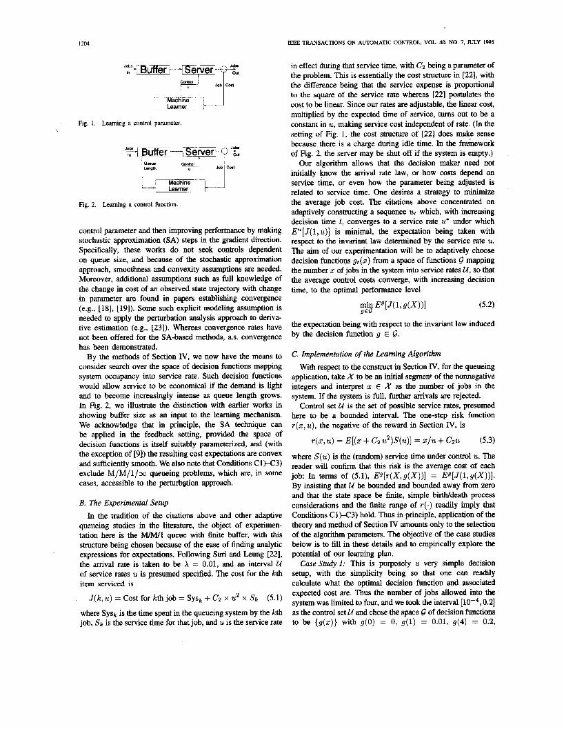
and vital application area for the developments in Section IV. A number of authors (e.g., [9], [18]-[22]) have considered the problem of adaptively adjusting a service rate parameter, call it U, on the basis of observed system times of customers and service costs. In Fig. 1, we illustrate the structure of the problem. Of the citations above, all but [9] are concerned with inferring the gradient of peafonnance with respect to the

IEEE TRANSACTIONS ON AUTOMATIC CONTROL, VOL. 40, NO. 7, JULY 1995

Fig. 1. Learning a control parameter.

Machine Learner

Fig. 2. Learning a control function.

control parameter and then improving performance by making stochastic approximation (SA) steps in the gradient direction. Specifically, these works do not seek controls dependent on queue size, and because of the stochastic approximation approach, smoothness and convexity assumptions are needed. Moreover, additional assumptions such as full knowledge of the change in cost of an observed state trajectory with change in parameter are found in papers establishing convergence (e.g., [18], [19]). Some such explicit modeling assumption is needed to apply the perturbation analysis approach to deriva- tive estimation (e.g., [23]). Whereas convergence rates have not been offered for the SA-based methods, a.s. convergence has been demonstrated.

By the methods of Section IV, we now have the means to consider search over the space of decision functions mapping system occupancy into service rate. Such decision functions would allow service to be economical if the demand is light and to become increasingly intense as queue length grows. In Fig. 2, we illustrate the distinction with earlier works in showing buffer size as an input to the learning mechanism. We acknowledge that in principle, the SA technique can be applied in the feedback setting, provided the space of decision functions is itself suitably parameterized, and (with the exception of [9]) the resulting cost expectations are convex and sufficiently smooth. We also note that Conditions C 1 >c3) exclude M/M/l /m queueing problems, which are, in some cases, accessible to the perturbgtion approach.

B. The Experimental Setup In the tradition of the citations above and other adaptive

queueing studies in the literature, the object of experimen- tation here is the M/M/l queue with finite buffer, with this structure being chosen because of the ease of finding analytic expressions for expectations. Following Suri and Leung [22], the arrival rate is taken to be X = 0.01, and an interval U of service rates U is presumed specified. The cost for the Lth item serviced is

(5.1) J (k ,v) = cost for kth job = Sys, + CZ x u2 x s k

in effect during that service time, with CZ being a parameter of the problem. This is essentially the cost structure in [22], with the difference being that the service expense is proportional to the square of the service rate whereas [22] postulates the cost to be linear. Since our rates are adjustable, the linear cost, multiplied by the expected time of service, turns out to be a constant in U, making service cost independent of rate. (In the setting of Fig. 1, the cost structure of [22] does make sense because there is a charge during idle time. In the framework of Fig. 2, the server may be shut off if the system is empty.)

Our algorithm allows that the decision maker need not initially know the arrival rate law, or how costs depend on service time, or even how the parameter being adjusted is related to service time. One desires a strategy to minimize the average job cost. The citations above concentrated on adaptively constructing a sequence ut which, with increasing decision time t, converges to a service rate U* under which E"[J( 1, U)] is minimal, the expectation being taken with respect to the invariant law determined by the service rate U.

The aim of our experimentation will be to adaptively choose decision functions gt(.) from a space of functions Q mapping the number z of jobs in the system into service rates U, so that the average control costs converge, with increasing decision time, to the optimal performance level

the expectation being with respect to the invariant law induced by the decision function g E 9.

C. Implementation of the k a m i n g Algorithm With respect to the construct in Section N, for the queueing

application, take X to be an initial segment of the nonnegative integers and interpret 2 E X as the number of jobs in the system. If the system is full, further k v a l s are rejected.

Control set U is the set of possible service rates, presumed here to be a bounded interval. The one-step risk function r (z , U) , the negative of the reward in Section IV, is

T ( Z , U ) = E[(. + c, U2)S(U) ] = ./U + CZU (5.3) where S(U) is the (random) service time under control U. The reader will confirm that this risk is the average cost of each job: In terms of (5.1), Eg[r(X,g(X))] = Eg[J(l,g(X))]. By insisting that U be bounded and bounded away from zero and that the state space be finite, simple birth/death process considerations and the finite range of r ( . ) readily imply that Conditions Cl)-c3) hold. Thus in principle, application of the theory and method of Section IV amounts only to the selection of the algorithm parameters. The objective of the case studies below is to fill in these details and to empirically explore the potential of our learning plan.

Case Study I: This is purposely a very simple decision setup, with the simplicity being so that one can readily calculate what the optimal decision function and associated expected cost are. Thus the number of jobs allowed into the system was limited to four, and we took the interval 0.21

where Sysk is the time spent in the queueing system by the Lth job, s k is the service time for that job, and U is the service rate

the control set U and chose the space 6 of decision functions to be {g(z)} with g(0) = 0, g(1) = 0.01, g(4) = 0.2,

LAI AND YAKOWITZ: NONPARAMETRIC BANDIT THEORY 1205

and g(2).9(3) E (lW4,0.2), g(2) < g(3). As prescribed in

random; g2(2) and g,(3) are taken to be the minimum and maximum, respectively, of the set of pairs {Ut(l), U,(2)} the elements of which are uniformly selected from U, the selection being independent for each i, and independent in 1:. The implementation of the algorithm was direct and in no way makes use of the M/M/l/K structure. The parameters were chosen to be

nt := 2',

Section IV-B, the functions g2, i = 1,2, ..... are selected at

for i 5 8, Lilog,(i)]. 1: > 8,

An2 := ln(i) (in the construction (2.2)), CZ := 2500 (value of service cost parameter in (5.1)). (5.4)

The set of bandit arms (decision functions chosen) is aug- mented only at "big-block" times nl, so k, and A, are not defined at other times. The reader will be able to confirm that the hypotheses of Section IV-B are satisfied by the simple bounded queueing decision model and the learning algorithm with parameters as in (5.4). We have chosen the M/M/l/K queueing problem to be able to compute theoretical risks Eg[r (X , g ( X ) ) ] conveniently by numerical matrix analysis. Having done so, by a simple application of mathematical programming, we established that the best operating point is approximately

(g( l ) , g(2), 9(3),9(4)) = (0.0L0.018,0.019,04

the expected cost being about 3.15, for each job. In Fig. 3, we show on-line running average cost-per-job

curves ( l /n Cy=l J ( X ( t ) , t ) ) , on different time scales, for a single learning session. Also the panels depict the expected costs of the best bandit arm located at the indicated time, i.e.,

min Eg' J ( 1. gi ( X ) ) . {i:ns.Ln}

(This curve is, of course, a decreasing step function. The slope in the 200-job curve in the top panel is a consequence of plotting routine interpolation.)

By these curves, one sees the balancing of the two forms of error: i) the performance of the best arm thus far gathered falling short of the optimal performance and ii) the increased cost over even that arm because perhaps it has not yet been detected as being the best, and/or because the rule (4.2) calls for the forced sampling of even worse arms.

In Fig. 4, we have exhibited the results of three additional queue learning sessions. Ow experience is that these curves are somewhat typical of performance on this small problem. There are four or five improvements in the expected cost of the best arm located at different times during a session, and after a few thousand jobs, the best arrn performances and the overall average costs are not far from the ideal, which is approximately 3. WJob.

Case Study 2: We enlarge the preceding queue decision problem to an occupancy of up to 11 levels, i.e., X = {0,1, ... ,lo}. The functions g E E are monotone increasing and range again in U = [10-4,0.2]. Functions are chosen at

Sample Average CosUJob

..................... '"""'. ... ................................... '

Best Sampkd Arm Theontical COrVJob

8 2

1m 1 y I m No. of Jobs Completed

CcsVJob

No. of Jobs = Zoo0

3 5 - : ........................................................................ Best Sampbd Am. Theoretical CoWJob

s - - - -L I

m 1 .mo 1 .m 2 No. of Jobs Completed

CMJob - - I I

No. of Jobs=13o,OW 5i m

Sample Average CosUJob 'I K p l e d Arm Theoret; CostlJob

3 5 ......... ................................................................

3 -L- "o a~ am m k t m : m 4 c c a

No. of J o b Completed

Average and best-arm costs for the five-state controlled queue. Fig. 3.

random from 0 by setting g(0) = 0, g( 1) and g( 10) to be the lower and upper endpoints of U, and taking g( j ) , j = 2,. .. ,9, to be the ordered sample of eight uniform observations from the sample space U. The scaling of the service cost was increased to CZ = 40000 to force a trade-off between service rate and queue length that caused longer queues to be cost effective, thus making the search for optimality more challenging. The authors did not attack the somewhat formidable task of finding the true optimum of €he resulting problem, which involves finding the minimum of an eight- variable constrained nonlinear function.

Fig. 5 shows the running average cost per job and expected performance of the best arm sampled during three consecutive learning sessions which use the same algorithm as employed for the first case study. Toward assuring the reader that there is some regularity in learning performances for this queue control problem, in Table I we have listed the expected costs at the best arm and average performances of an additional 10 successive learning replications, after 130000 jobs.

I206

CostlJob

30-

25

No of Jobs=130,000 5 +

Sample Average CosWJob

Best Sampled Arm Theoretical CosVJob 35

...................................................................... 3 - A---- A-

moo0 “0 80.m som 1” 120,m 14

NO of Jobs Completed

-

a

Best Sarnpbd Arm: Theoreticdl CosWJob Sample Average CosWJob

-21

CosffJob

55r- 1 No. of Jobs=130,000 ~

Sample Average CosWJob

Best Sampled Arm: Thewst i l CosVJob

36 p P .................................... ~ ..................................... t

3 L - 2om 8 o ~ m k i m ~ idmdax

No of Jobs Completed

CosVJob

1

No of Jobs=130,000

Sample Average CosWJob 4:c Beat Samp!ed Ann Theoretical CwVJob

35;

i i .......... A ...........................................................

2o.m yl.m m.mo m.m imam 120.m 1aomo 3 L 1

NO. of Jobs Completed

Fig. 4. five-state controlled queue.

Average and best-arm costs of three learning sessions for the

It is evident that the trajectories have more variability in this expanded case. But also, clearly, adaptive improvement is taking place, and this is the feature we hold particularly significant.

VI. PROOF OF THEOREMS 3 AND 4 The proof of Theorems 3 and 4 uses martingale theory. For

n 2 0, let 3, denote the a-field generated by {g1,92, . . -} U { (&, Xt), 1 5 t 5 n}, where 4 denotes the adaptive control rule of Theorem 3 (or 4) and q5t is the control law in 8 which q5 uses at time t. Note that the gt are nonrandom in Theorem 3 but are random and &-measurable in Theorem 4. Let d be a positive integer. The adaptive control rule 4 of Theorem 3 or 4 uses the same stationary control law for an entire block of stages v,(m). .... vz(m + 1) - 1, with the choice of the control law determined at the beginning of the block via (4.2). Therefore, for vz(m) + d - 1 5 t < vE(m + 1) and g E 8,

IEEE TRANSACTIONS ON AUTOMATIC CONTROL, VOL. 40, NO. 7, JULY 1%

CosVJob 40

7 No ofbbs=130,000 I

0

Sample Average CasVJob

&st Sampk! Arm: Theoretiml CosVJob 10

20.m a,m mmo w,mo impm imm i40mo No. of JO$S Completed

CosVJob

No. of Jobs=130,MX)

forall n 2 D. (6.2)

Define a sequence {h;} of positive integers such that D 5 hi - h,-l 5 20 - 1 and all the vt(m) with t 2 D belong to the sequence. For example, take ho = 1, hl = n D and for i > 1 let h, = hi-1 + D except when h, = vt(m), for which we may change the above recursive definition of hi to h, = h,-l + D + T , with 0 5 T < D being the remaindm obtained when vt(m) - vt(m - 1) is divided by D. Since the adaptive control rule 4 of Theorem 3 or 4 chooses the same

LA1 AND YAKOWITZ: NONPARAMETRIC BANDIT THEORY lUn

TABLE I THE EXPECTED COSTS AT THE BEST OBSERVED ARMS AND THE AVERAGE COSTS, FOR 10 LEARNING SESSIONS OF 130000 JOBS

Thm. Val. at Beat Arm I Average Cost/Job I Efficiency

I 14.2 I 0.958 2 3 4 5 6 1 8 9 10

13.9 12.7 12.5 12.6 13.5 12.8 14.1 12.7 12.6

16 1 13 6 13 6 13 0 1s 6 13 9 14 5 13 4 13 0

0.863 0.934 0.919 0.969 0.865 0.921 0.912 0.948 0.969

t + 4 0 - 2. Let

i=l s=h,-1

i=l

control law for hi-1, . a . , ha - 1 on the basis of observations prior to stage hi-1, it follows from (6.2) and an argument similar to (6.1) that

Then { $J), B~~ ( 3 ) , t 2 1 ) is a martingale. Since {gt(j) = r ) E Br-l, it follows from (6.4) that

/ \ 4

I h,-1

Let Y , -- - E;:i,l-l . (Xt,+t(Xt)) + E,[E:& .(Xt, q5t(Xt))lFht-l-1]. Then {yZ,B,,Z 2 1) is a martingale dif- ference sequence, where Bt = Fh,-l. Moreover, by C2) and an argument similar to (6.1)

2 0 - 1

noting that (c;;i:-l ut)4 5 (hi - hi-1)3Ct:;;tI a: and that hi - hi-1 5 2 0 - 1. Similarly, by C3) and the CauchySchwarz inequality

2 0 - 1

Therefore by Doob's martingale inequality, for any 6 > 0, P,{maxtSml~t(3)l 2 6m) 5 (sm)-4qsF14 = 0(m-2),

uniformly in j. Hence

= o(2-2") = 0(m-2) u:2">m

for any S > 0. Combining this with (6.3) yields

- r ( x d , g ( x d ) ) ) ) ~ ~ - ? < cc for o < < I 0/2d. which is analogous to A3). Similarly with E in (6.3) sufficiently small, it follows from (6.5) and Remark 1 of Section 11 that there exist y > 0,O < q < A* -supggL Ag and c > 0 such that

(6*5)

Since q5t = q!%,.-l for ha-1 5 t < ha and { q ! ~ t , - ~ = g3} E

F h , - l - ~ = B t - l . { C , n = 1 Y z l ~ ~ h , _ , = g 3 } , B ~ . n 2 1 ) is a martingale, not only in Theorem 3 but also in Theorem 4 in which the g3 are &-measurable random functions.

at(.?) h,-1

t=1 s=h,-l g, E~ .

t

- A* < -q = O(e-Yt), (6.8) I Proof of Theorem 3: For fixed j, define an increasing sequence of stopping times ot(j) = inf{i 2 l : ~ ~ ( h ~ - ~ ) 2 t } , t 2 1. Since D 5 hi - hi-1 I 2 0 - 1,t 5 ~ ~ ( h ~ * ( ~ ) ) 1.

1208 IEEE TRANSACTIONS ON AUTOMATIC CONTROL, VOL. 40, NO. 7, JULY 1

by P,(.l.Fo). Therefore (6.10) still holds, and analogous to (3.4) and (6.11), we now have

I

in analogy with Al) and A2). Since by (4.3)

U t ( 3 ) h , -1

Z&) = (.MY G S , 9 j ( X S > )

t=1 s=h, - l

' { 4 h , - l = g , } if = ' U t ( j )

and since t 5 ~ ~ ( h ~ , ( ~ ) ) 5 t + 4 0 - 2 , the rest of the proof is similar to that of Theorem 2.

Note that (6.7) is somewhat stronger than A2), and using it instead of A2) gives the following sharper bound than (3.5) used in the proof of Theorem 2

by (3.1). This explains why (4.5) has the term k, [coming from (3.4)] instead of IC: that would have come from (3.5). Moreover, (6.7) enables us to replace (3.6) by the sharper result

ni+i

(6.11) 3 = l

This sharper result is needed here because at a stage n when g j is used, with n 5 ni+1 and ~ ~ ( n ) = T, the decision to use g j may be based on a dest per fomd at several stages before n since our rule involves testing only at the beginning of each block of stages. Note that the sizes of these blocks are dominated by half of the total number ~ ~ ( h ~ ~ ( j ) ) of times gJ is used, for sufficiently large t , which explains the range T / 2 5 t 5 T in the event in (6.11). Moreover, if

0 Proof of Theorem 4: Since G = 91, g2, . .} is a random

set that is &-measurable and since { Sf'), But ( j ) , t 2 1) is still a martingale, (6.7x6.9) remain valid if we replace P, there

nu 5 b t ( j ) < n u + l with 5 2 , then h v , T , ( h m t ( , ) ) 5 %,,t and (6.1 1) uses this upper bound.

i=l s=hi-l

in which 0 < 7 < E - 6'. Moreover, by (4.7), P,{gj 6 L for all j 5 kn,+} = o(n;'), for every fixed positive integer v. Hence we can again modify the proof of Lemma 1 and Theorem 34) of Lai and Robbins [4] to complete the proof.

VII. CONCLUSION The first three sections of this work are devoted to extending

and improving upon known results about nonparametric, non- Bayesian bandit theory for i.i.d. observat;ans to situations in which observables depend on the past history of the same bandit arm. They provide the sharpest results and under the weakest assumptions to date on nonparametric bandit theory. The bandit problems considered can use observations of processes having complex dynamics of unknown structure. Under conditions we have offered, convergence at given rates is assured, even in the presence of noise which is dependent on controls and history. The learning methodology side-steps the need to model the process.

The study of nonparametric bandit theory provides the back- ground for another task of real interest (Section IV): learning for controlled Markov decision processes. The methods here had precursors in [7] (for finite state processes) and 191 (which did not explicitly recognize that the search could be over a function space). The rates of negret convergence established in the present work are equal or close to what is achievable even in the most restrictive i.i.d. cases. Simple Computational illustrations were offered which indicate that learning decision functions (of buffer size) for controlled queues is possible. To our knowledge, reports of such a computational study have not appeared before. The bandit theory approach to learning is almost a black-box method in that it is entirely data-driven; subsequent inputs are determined entirely on the history of input-output pairs, with the inputs being decision functions and the outputs being performance values, exclusively. By

LAI AND YAKOWITZ: NONPARAMETRIC BANDlT THEORY 1209

way of practical use of leaming, we foresee designers using

uate control policies before putting them on-line for process

[18] E. K. P. Chong and P. J. Ramadge, “Optimization of queues using an infinitesimal perturbation analysis-based stochastic algorithm with

1993.

traditional methods and available statistics to develop and eval- general update times,” J. Confr. optim., vol. 31, pp. 698-732,

control. Once operation begins, learning methods such as those related here can be employed to fine-tune the performance as the database grows by choosing the control policy which is most appropriate for the situation.

The authors hope that the methodology and theoretical tools offered here may be useful as an altemative to the better- known stochastic approximation (SA)-perturbation analysis (PA) avenue. There one relies on smoothness and convexity assumptions for expected cost as a function of parameters. Moreover, those methods proven to be convergent are based on PA estimation of derivatives, and PA, in turn, requires very explicit modeling assumptions.

REFERENCES

S . Yakowitz, Mathematics of Adaptive Control Processes. New York Elsevier, 1969. D. A. Berry and B. Fristedt, Bandit Problems. London: Chapman and Hall, 1985. H. Robbins, “Some aspects of the sequential design of experiments,” Bull. Amer. Math. Soc., vol. 55, pp. 527-535, 1952. T. L. Lai and H. Robbins, “Asymptotically efficient adaptive allocation rules,” Adv. Appl. Math., vol. 6, pp. 4-22, 1985. C. L. &lallows and H. Robbins, “Some problems of optimal sampling strategy,” J. Math. Anal. Appl., vol. 8, pp. 90-103, 1964. S. Yakowitz and W. Lowe, “Nonpamnetric bandit methods,’’ Ann. Operat. Res., vol. 28, pp. 297-312, 1991. R. Agrawal, D. Teneketzis, and V. Anantharam, “Asymptotically effi- cient adaptive allocation schemes for controlled Markov chains: Finite parameter space,” IEEE Trans. Automr. Contr., vol. 34, pp. 1249-1259, 1989. T. Graves and T. L. Lai, “Asymptotically efficient adaptive choice of control laws in controlled Markov chains,” SIAM J. Contr., to appear. S. Yakowitz, T. Jayawardena, and S. Li, “Theory for automatic leam- ing under partially observed Markov-dependent noise,” IEEE Trans. Automat. Contr., vol. 37, pp. 1316-1324, 1992. T. L. Lai and Z. Ying, “Parallel recursive algorithms in asymptotically efficient adaptive control of linear stochastic systems,” SIAM J. Confr. Optim., vol. 29, pp. 1091-1127, 1991. V. Anantharam, P. Varaiya, and I. W h d , “Asymptotically efficient allocation rules for multiarmed bandit problem with multiple plays. P m II: Markovian Rewards,” IEEE Trans. Automat. Contr., vol. 32, pp.

I. Iscoe, P. Ney, and E. Nummelin, “Large deviations of uniformly recurrent Markov additive processes,” Adv. Appl. Math., vol. 6, pp. 373-412, 1985. W. F. Stout, Almost Sure Convergence. New York Academic, 1974. T. Chiyonobu and S . Kusuoka, ‘“The large deviation principle for hypemixikig processes,” Probab. Theory Related Fields, vol. 78, pp. 627-649, 1988. R. H. Schonmann, ‘‘Ekpnentiah convergence under mixing,” Probab. Theory Related Fields, vol. 81, pp. 235-238, 1989. S. Orey and S. P e l i , “Large deviation principles for stationary processes,” Ann. Probab., vol. 16, pp. 1481-1495, 1988. W. Bryc and A. Dembo, “Large deviations and strong mixing,” Dept. Statistics, Stanford Univ., Tech. Rep., 1993.

975-982, 1987.

1

[19] H. 3. Kushner and F. VBzquez-Abad, “Stochastic approximation methods for systems of interest over an infinite horizon,” SIAMJ. Contr. Optim., submitted, 1994.

[20] P. L‘Ecuyer and P. W. G l y ~ , ‘‘Stochastic optimization by simulation: Numerical experiments for a simple queue in steady state,” Manag.

[21] G. C. Pflug, “On-line optimization of simulated Markovian processes," Math. Operat. Res., vol. 12, pp. 381-395, 1990.

[22] R. Suri and Y. T. bung, “Single-run optimization of discrete-event simulations: An empirical study using the W 1 queue,” Trans. Inst. Industrial Eng., vol. 21, pp. 3549, 1989.

[23] F. Vwuez-Abad and H. J. Kushner, “Estimation of the derivative of a stationary measure with respect to a control parameter,” J. Appl. Probab., vol. 29, pp. 343-352, 1992.

Sci., vol. 40, pp. 1562-1578, 1994.

Tm-Le- JA was bom in Hong Kong in 1945. He received the B.A. degree in mathematics from the University of Hong Kong in 1967 and the Ph.D. degree in mathematical statistics from Columbia University, New York, in 1971.

Since 1987, he has been a Professor of Statistics at Stanford University, Stanford, CA. From 1971 to 1987, he was on the faculty of Columbia Univer- sity. He has held professorships at the University of Illinois and the University of Heidelberg. His current research interests are in adaptive control

and learning systems, sequential experimentation. stochastic optimization, probability theory, and biostatistics. Dr. Lai is a Fellow at the Institute of Mathematical Statistics and the Amer-

ican Statistical Association; he is a Member of the International Statistical Institute, the Biometric Society, and the Dmg Information Association. He was awarded a John Simon Guggenheim Fellowship (1983-1984) and the Committee of Presidents Statistical Societies Award (1983).

Sidney Yakonite (S.’58-M’75) was born in San Francisco, CA, in 1937. He received the B.S. degree in electrical engineering from Stanford University, Stanford, CA, and the Ph.D. degree in electrical engineering from Arizona State University, Tempe, in 1967.

Since 1966, he has been with the Systems and Industrial Engineering Department at the University of Arizona. His current research intgests include nonparametric estimation in the time series caw, machine leaming, and statistical and decision mod-

els for the AIDS epidemic. He is the author of the books, Mathematics of Adaptive Control Processes and Computational Probability and Simulation and co-author of Principles and Procedures of Numerical Analysis and An Introduction to Numerical Computations. Dr. Yakowitz is a member of SIAM, the Institute of Mathematical Sta-

tistics, and the American Statistical Association. He was a recipient of an NAS/NRC Post-Doctoral Fellowship at the U.S. Naval Postgraduate School in 1970-1971.