Machine Learning and Big Data Analytics in Power ...
106
Machine Learning and Big Data Analytics in Power Distribution Systems Prof. Nanpeng Yu Department of Electrical and Computer Engineering Department of Computer Science and Department of Statistics (cooperating faculty) [email protected] 951.827.3688
Transcript of Machine Learning and Big Data Analytics in Power ...

Machine Learning and Big
Data Analytics in Power
Distribution Systems
Prof. Nanpeng Yu
Department of Electrical and Computer
Engineering
Department of Computer Science and
Department of Statistics
(cooperating faculty)
951.827.3688

Team Members
Center Director (Energy, Economics, and Environment)
Dr. Nanpeng Yu
Postdoctoral Scholar
Dr. Brandon Foggo (B.S. UCLA, Ph.D. UCR)
Ph.D. Students
Wei Wang (M.S. University of Michigan), Yuanqi Gao (B.S. UCR)
Wenyu Wang (M.S. Iowa State University), Farzana Kabir (B.S. BUET)
Jie Shi (M.S. Southeast University), Yinglun Li (M.S. UCR)
Osten Anderson (B.S. UCLA), Yuanbin Cheng (M.S. USC)
Xianghao Kong (B.S. HDU)
Current and Past Projects and Sponsors
Over 10 Million of Research and Development Projects as PI and Co-PI
DOE PMU Data Analytics (PI, DOE, $1 Million)
Distributed Energy Management System (PI, CEC, $1.2 Million)
Distribution System Operator Managed Electricity Market (PI, DOE, $0.45 Million)
Smart Cities (PI, NSF, $0.3 Million)
Water-Energy-Climate Nexus (PI, CEC, $0.45 Million)
Big Data Analytics and Machine Learning (PI, Electric Utilities, $0.3 Million)
Green Computing (PI, CEC, $1.8 Million)
DOE Education (Site-PI, DOE, $0.5 Million)

OutlineWhy do we focus on electric power distribution systems?
Big Data in Power Distribution Systems
Volume, Variety, Velocity, and Value
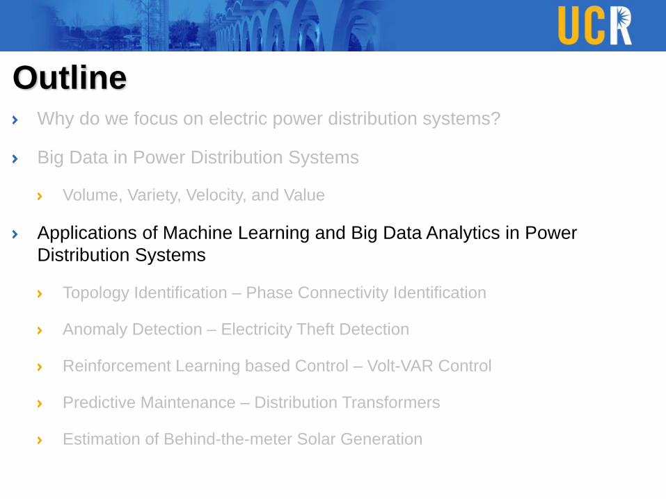
Applications of Machine Learning and Big Data Analytics in Power
Distribution Systems
Topology Identification – Phase Connectivity Identification
Anomaly Detection – Electricity Theft Detection
Reinforcement Learning based Control – Volt-VAR Control
Predictive Maintenance – Distribution Transformers
Estimation of Behind-the-meter Solar Generation
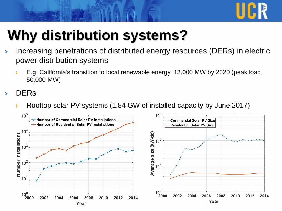
Why distribution systems?Increasing penetrations of distributed energy resources (DERs) in electric
power distribution systems
E.g. California’s transition to local renewable energy, 12,000 MW by 2020 (peak load
50,000 MW)
DERs
Rooftop solar PV systems (1.84 GW of installed capacity by June 2017)
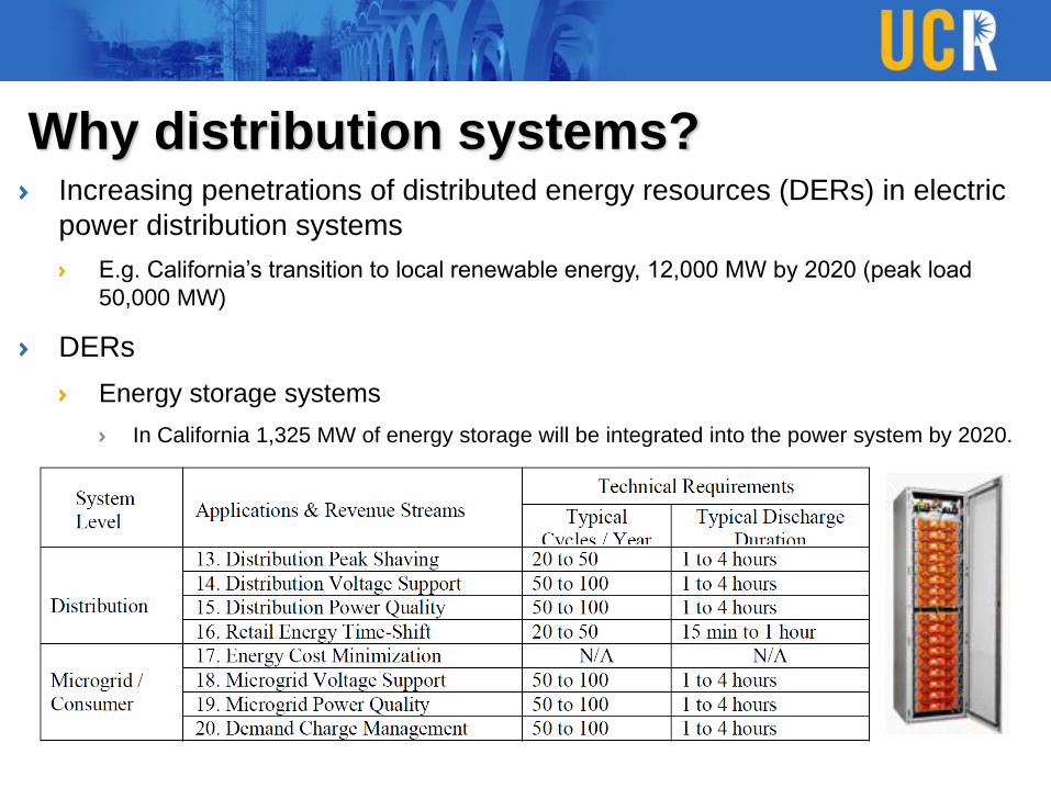
Why distribution systems?Increasing penetrations of distributed energy resources (DERs) in electric
power distribution systems
E.g. California’s transition to local renewable energy, 12,000 MW by 2020 (peak load
50,000 MW)
DERs
Energy storage systems
In California 1,325 MW of energy storage will be integrated into the power system by 2020.
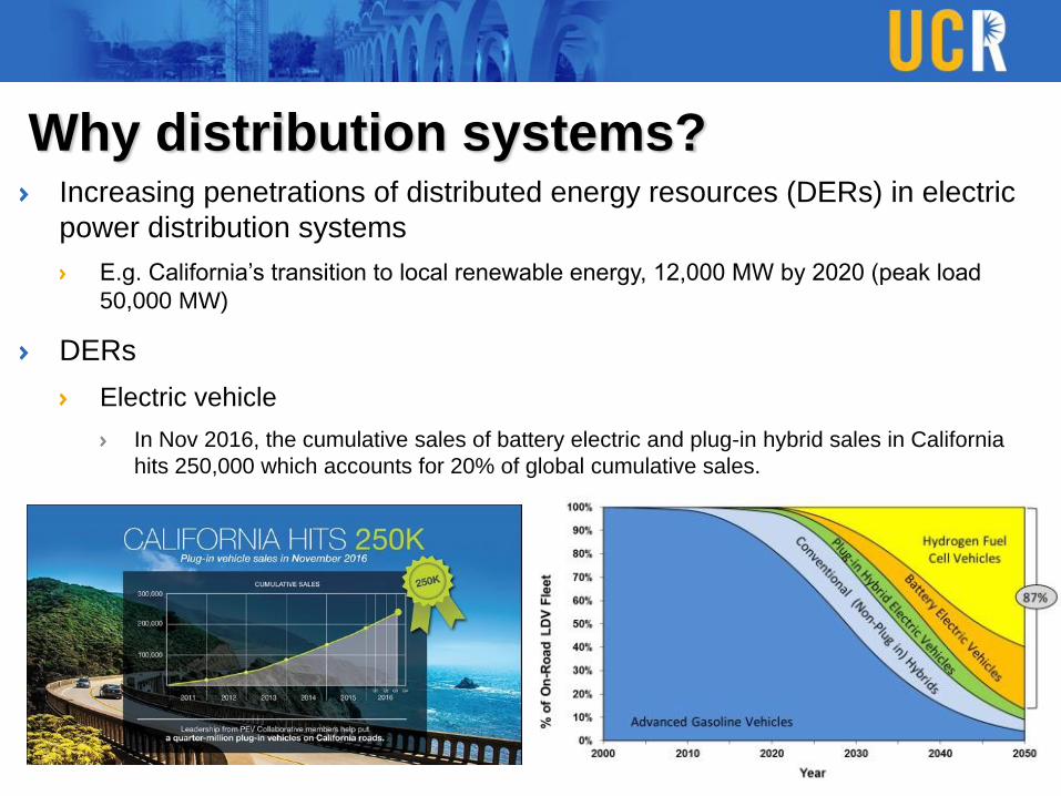
Why distribution systems?Increasing penetrations of distributed energy resources (DERs) in electric
power distribution systems
E.g. California’s transition to local renewable energy, 12,000 MW by 2020 (peak load
50,000 MW)
DERs
Electric vehicle
In Nov 2016, the cumulative sales of battery electric and plug-in hybrid sales in California
hits 250,000 which accounts for 20% of global cumulative sales.
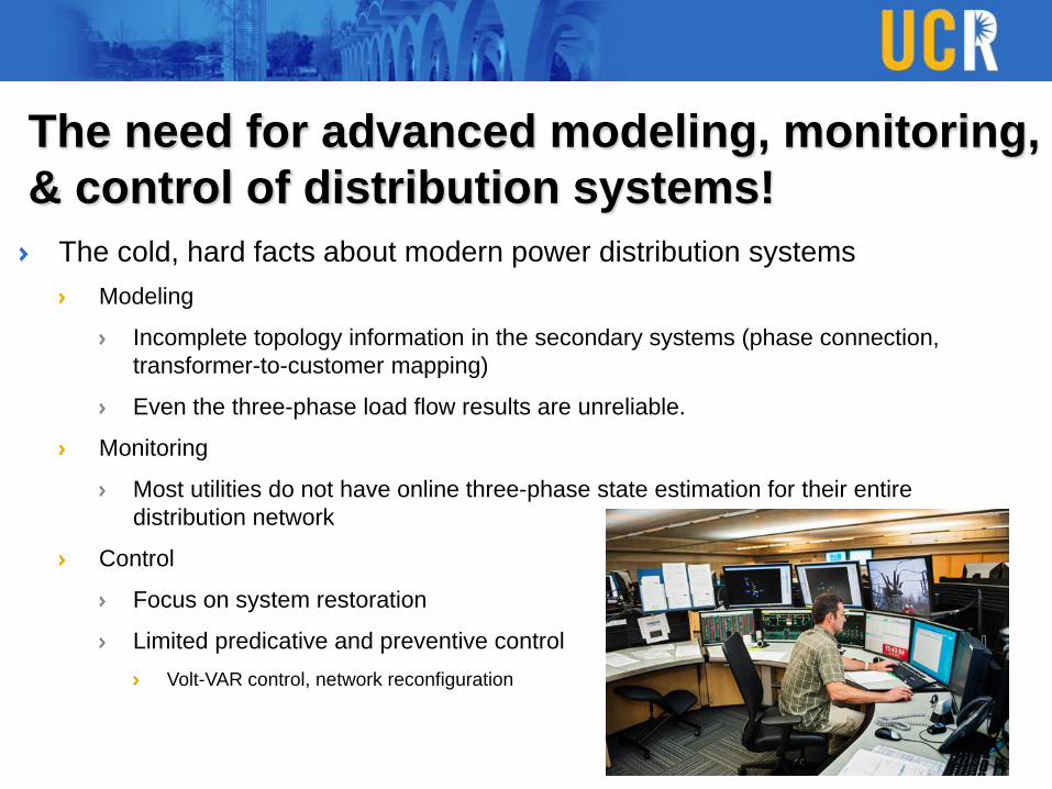
The need for advanced modeling, monitoring,
& control of distribution systems!
The cold, hard facts about modern power distribution systems
Modeling
Incomplete topology information in the secondary systems (phase connection,
transformer-to-customer mapping)
Even the three-phase load flow results are unreliable.
Monitoring
Most utilities do not have online three-phase state estimation for their entire
distribution network
Control
Focus on system restoration
Limited predicative and preventive control
Volt-VAR control, network reconfiguration

OutlineWhy do we focus on electric power distribution systems?
Big Data in Power Distribution Systems
Volume, Variety, Velocity, and Value
Applications of Machine Learning and Big Data Analytics in Power
Distribution Systems
Topology Identification – Phase Connectivity Identification
Anomaly Detection – Electricity Theft Detection
Reinforcement Learning based Control – Volt-VAR Control
Predictive Maintenance – Distribution Transformers
Estimation of Behind-the-meter Solar Generation
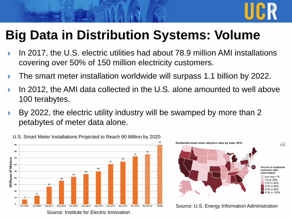
Big Data in Distribution Systems: Volume
In 2017, the U.S. electric utilities had about 78.9 million AMI installations
covering over 50% of 150 million electricity customers.
The smart meter installation worldwide will surpass 1.1 billion by 2022.
In 2012, the AMI data collected in the U.S. alone amounted to well above
100 terabytes.
By 2022, the electric utility industry will be swamped by more than 2
petabytes of meter data alone.
Source: U.S. Energy Information Administration
U.S. Smart Meter Installations Projected to Reach 90 Million by 2020
Source: Institute for Electric Innovation

Advanced Metering Infrastructure
Electricity usage (15-minute, hourly)
Voltage magnitude
Weather Station
Geographical Information System
Census Data (block group level)
Household variables: ownership, appliance, # of rooms
Person variables: age, sex, race, income, education
SCADA Information
Micro-PMU
Time synchronized measurements with phase angles
Equipment Monitors
Wireless
Network
Cell Relay
RF
Neighborhood
Area Mesh
Network
Wide-Area Network
Meter Data
Management
System
Big Data in Distribution Systems: Variety

Big Data in Power Distribution Systems:
VelocitySampling Frequency
AMI’s data recording frequency increases from once a month to one reading every 15
minutes to one hour.
Micro-PMU hundreds (512) of samples per cycle at 50/60 Hz
Bottleneck in Communication Systems (Distribution Network)
Limited bandwidth for zigbee network
Most of the utilities in the US receives smart meter data with ~24 hour delay
Edge Computing Trend
Itron and Landis+Gyr extend edge computing capability of smart meters
Increasing data transmission range and computing capabilities of smart meters
Centralized → distributed / decentralized
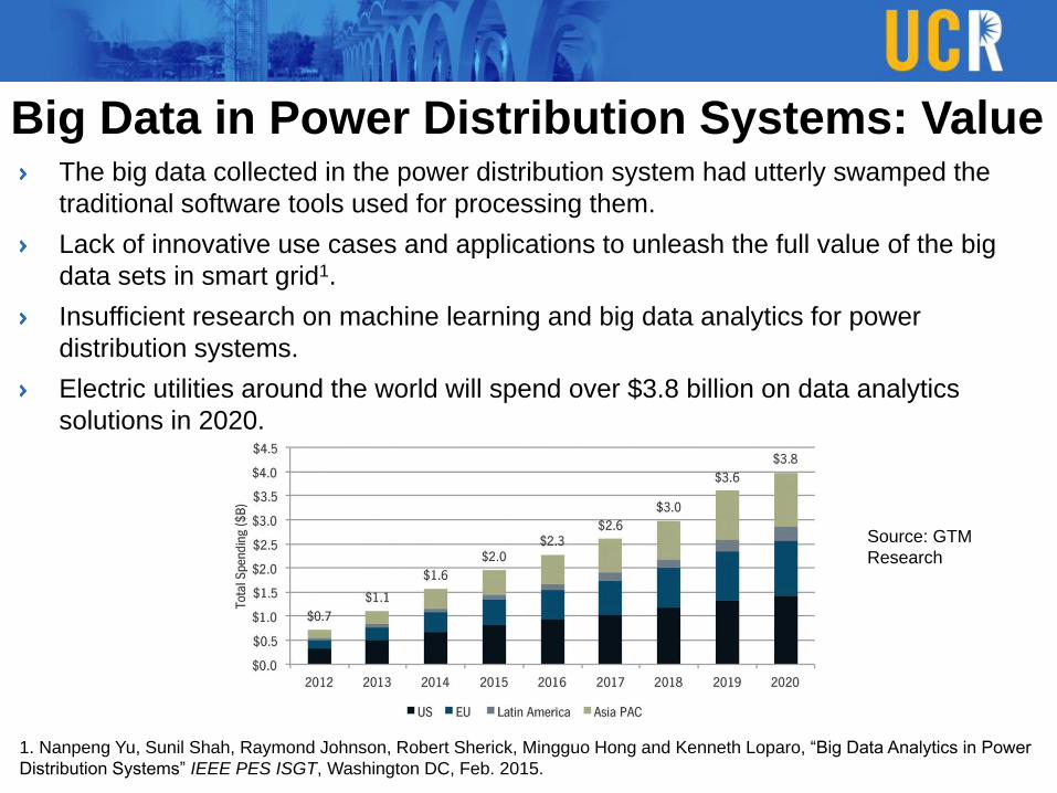
Big Data in Power Distribution Systems: ValueThe big data collected in the power distribution system had utterly swamped the
traditional software tools used for processing them.
Lack of innovative use cases and applications to unleash the full value of the big
data sets in smart grid1.
Insufficient research on machine learning and big data analytics for power
distribution systems.
Electric utilities around the world will spend over $3.8 billion on data analytics
solutions in 2020.
1. Nanpeng Yu, Sunil Shah, Raymond Johnson, Robert Sherick, Mingguo Hong and Kenneth Loparo, “Big Data Analytics in Power
Distribution Systems” IEEE PES ISGT, Washington DC, Feb. 2015.
Source: GTM
Research
OutlineWhy do we focus on electric power distribution systems?
Big Data in Power Distribution Systems
Volume, Variety, Velocity, and Value
Applications of Machine Learning and Big Data Analytics in Power
Distribution Systems
Topology Identification – Phase Connectivity Identification
Anomaly Detection – Electricity Theft Detection
Reinforcement Learning based Control – Volt-VAR Control
Predictive Maintenance – Distribution Transformers
Estimation of Behind-the-meter Solar Generation
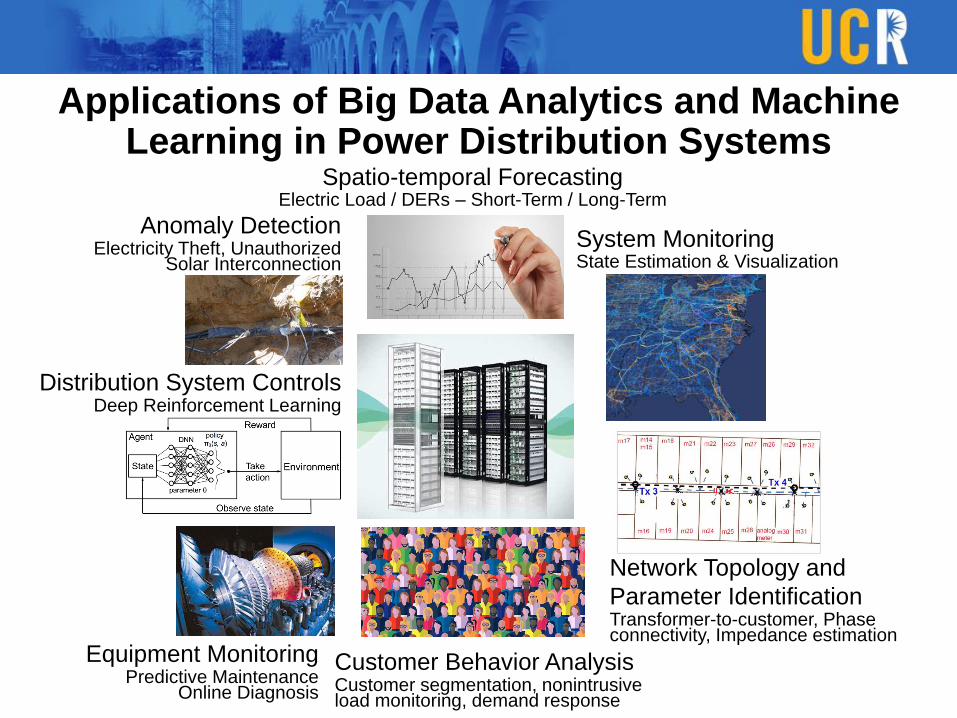
Applications of Big Data Analytics and Machine Learning in Power Distribution Systems
Spatio-temporal ForecastingElectric Load / DERs – Short-Term / Long-Term
Anomaly DetectionElectricity Theft, Unauthorized
Solar Interconnection
Equipment MonitoringPredictive Maintenance
Online Diagnosis
System MonitoringState Estimation & Visualization
Network Topology and
Parameter IdentificationTransformer-to-customer, Phase connectivity, Impedance estimation
Customer Behavior AnalysisCustomer segmentation, nonintrusive load monitoring, demand response
Distribution System ControlsDeep Reinforcement Learning

OutlineWhy do we focus on electric power distribution systems?
Big Data in Power Distribution Systems
Volume, Variety, Velocity, and Value
Applications of Machine Learning and Big Data Analytics in Power
Distribution Systems
Topology Identification – Phase Connectivity Identification
Anomaly Detection – Electricity Theft Detection
Reinforcement Learning based Control – Volt-VAR Control
Predictive Maintenance – Distribution Transformers
Estimation of Behind-the-meter Solar Generation
Phase Identification
Phase Connectivity Identification
Unsupervised Machine Learning
Linear dimension reduction and centroid-based clustering
Nonlinear dimension reduction and density-based clustering
Supervised Machine Learning
A comprehensive evaluation of supervised machine learning algorithms
Improvement with the theory of information losses

Distribution System Topology Identification
18
The distribution system topology identification problem can be broken
down into two sub-problems
The phase connectivity identification problem
The customer to transformer association problem
Phase Connectivity Identification
Problem Definition
Identify the phase connectivity of each customer & structure in the power
distribution network.
Very few electric utility companies have completely accurate phase connectivity
information in GIS!
Why is it important? (Business Value)
Phase connectivity is crucial to an array of distribution system analysis &
operation tools including
3-phase Power flow
Load balancing
Distribution network state estimation
3-phase optimal power flow
Volt-VAR control
Distribution network reconfiguration and restoration
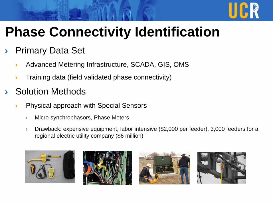
Phase Connectivity Identification
Primary Data Set
Advanced Metering Infrastructure, SCADA, GIS, OMS
Training data (field validated phase connectivity)
Solution Methods
Physical approach with Special Sensors
Micro-synchrophasors, Phase Meters
Drawback: expensive equipment, labor intensive ($2,000 per feeder), 3,000 feeders for a
regional electric utility company ($6 million)
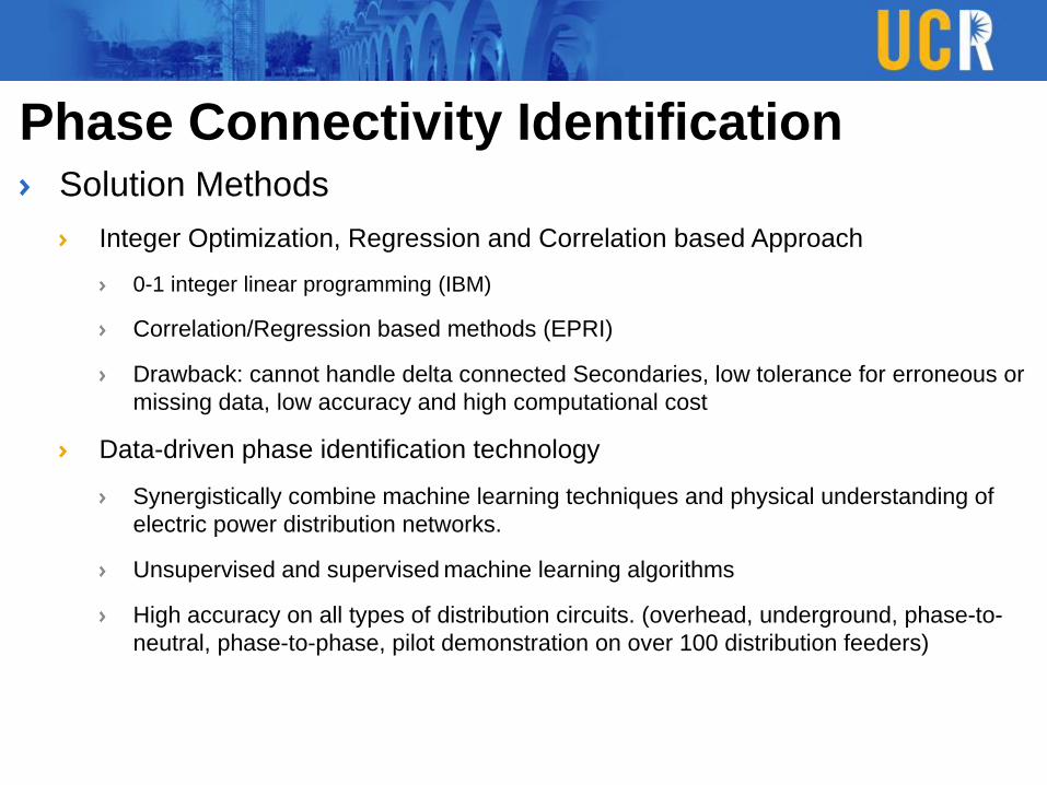
Phase Connectivity IdentificationSolution Methods
Integer Optimization, Regression and Correlation based Approach
0-1 integer linear programming (IBM)
Correlation/Regression based methods (EPRI)
Drawback: cannot handle delta connected Secondaries, low tolerance for erroneous or
missing data, low accuracy and high computational cost
Data-driven phase identification technology
Synergistically combine machine learning techniques and physical understanding of
electric power distribution networks.
Unsupervised and supervised machine learning algorithms
High accuracy on all types of distribution circuits. (overhead, underground, phase-to-
neutral, phase-to-phase, pilot demonstration on over 100 distribution feeders)
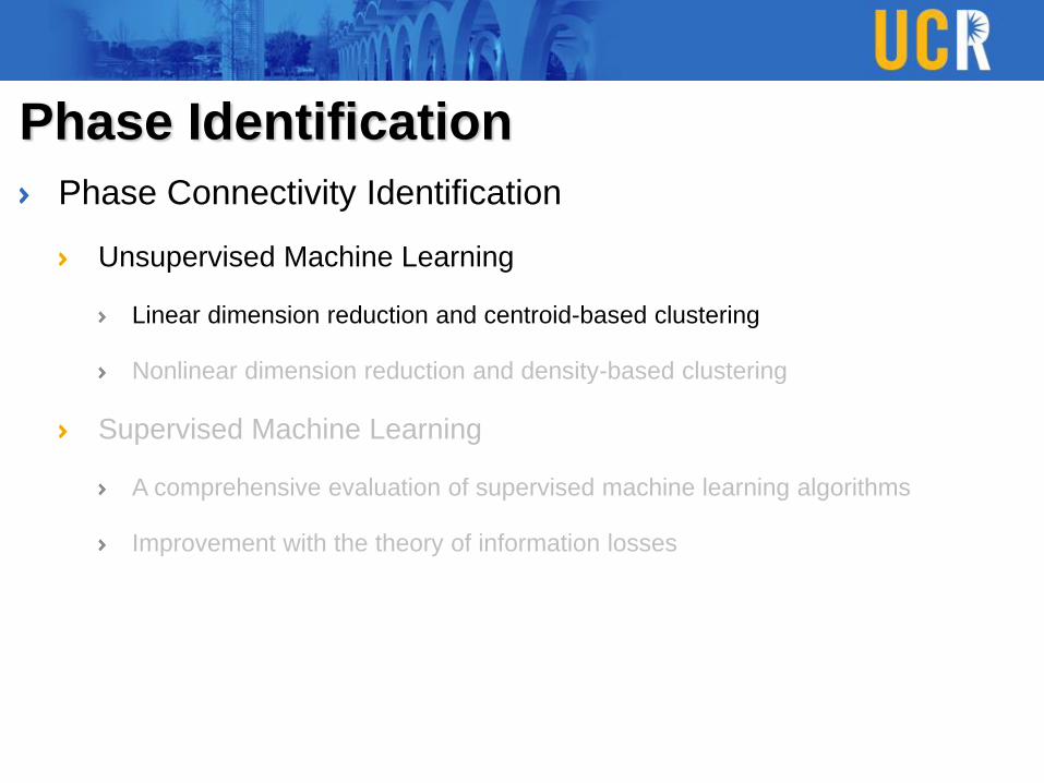
Phase Identification
Phase Connectivity Identification
Unsupervised Machine Learning
Linear dimension reduction and centroid-based clustering
Nonlinear dimension reduction and density-based clustering
Supervised Machine Learning
A comprehensive evaluation of supervised machine learning algorithms
Improvement with the theory of information losses
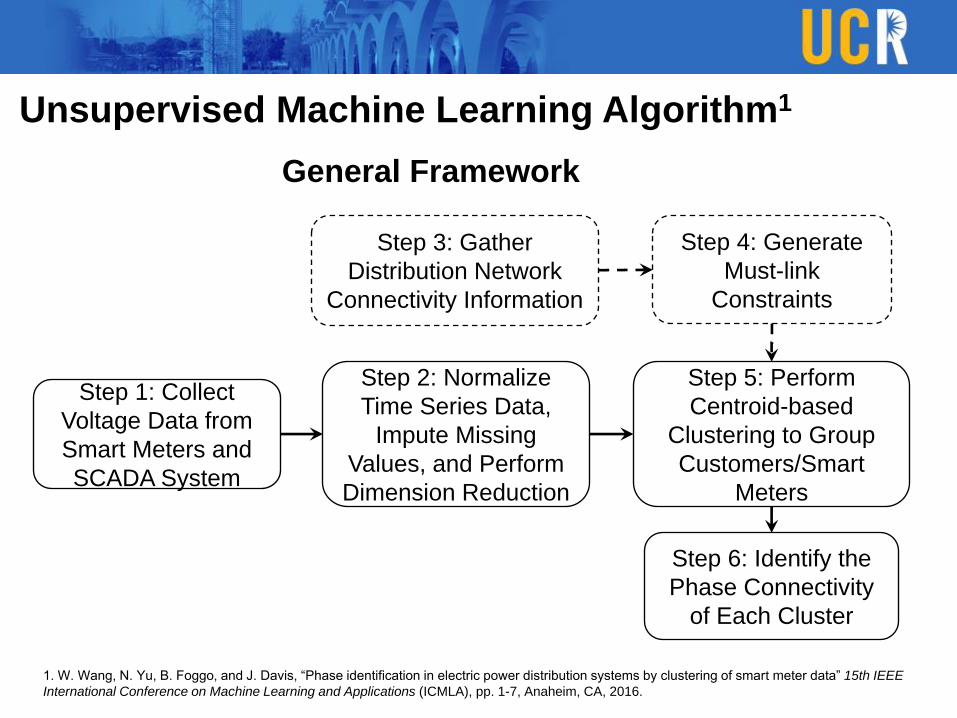
Unsupervised Machine Learning Algorithm1
General Framework
Step 1: Collect
Voltage Data from
Smart Meters and
SCADA System
Step 2: Normalize
Time Series Data,
Impute Missing
Values, and Perform
Dimension Reduction
Step 5: Perform
Centroid-based
Clustering to Group
Customers/Smart
Meters
Step 3: Gather
Distribution Network
Connectivity Information
Step 4: Generate
Must-link
Constraints
Step 6: Identify the
Phase Connectivity
of Each Cluster
1. W. Wang, N. Yu, B. Foggo, and J. Davis, “Phase identification in electric power distribution systems by clustering of smart meter data” 15th IEEE
International Conference on Machine Learning and Applications (ICMLA), pp. 1-7, Anaheim, CA, 2016.

Why Voltage Data Is Predictive of Phase?
Voltage data is fairly informative of phase type
Consider a power injection at bus 𝑘 whose phase type
is 𝐴𝐵.
This induces a current along the lines 𝐴 and 𝐵.
Any customer also feeding from either of those lines
will notice a change.
Due to the capacitive and inductive effects of the
primary feeder, both lines will also induce a voltage
change along the lines 𝐶 and 𝑛.
However, the off-diagonal elements of the phase
impedance and shunt admittance matrices are much
smaller than the diagonal ones.
Hence, the power injection at bus 𝑘 will have much less
effect on phase 𝐶 than phase 𝐴 and 𝐵.
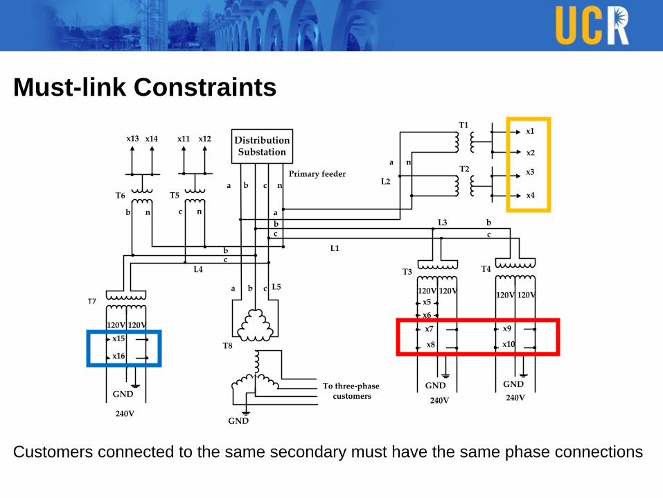
Must-link Constraints
DistributionSubstation
a b c n
a
b c
a n
b
c
a b c
b
b n
c
Primary feeder
L1
L2
L3
L4
c n
L5 120V 120V 120V 120V
120V 120V
240V
240V 240V
T1
T2
T3 T4
T5T6
T7
T8
x1
x2
x3
x4
x5
x6
x11 x12x13 x14
x10
x9
To three-phase customers
GND
GNDGND
x15
x16
x8
x7
GND
Customers connected to the same secondary must have the same phase connections
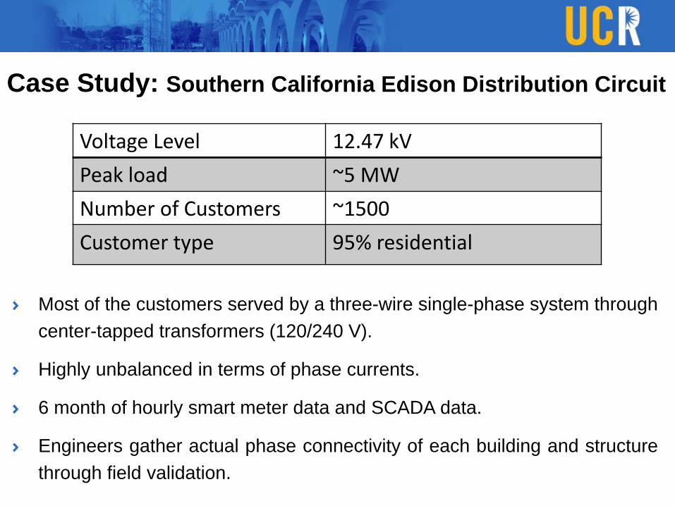
Case Study: Southern California Edison Distribution Circuit
Voltage Level 12.47 kV
Peak load ~5 MW
Number of Customers ~1500
Customer type 95% residential
Most of the customers served by a three-wire single-phase system through
center-tapped transformers (120/240 V).
Highly unbalanced in terms of phase currents.
6 month of hourly smart meter data and SCADA data.
Engineers gather actual phase connectivity of each building and structure
through field validation.

Unsupervised Learning: Unconstrained Clustering
Phase Identification Accuracy: 92.89%
Cluster
number
Number of
customers
Accuracy
(%) Phase
1 226 94.25 CA
2 647 95.21 AB
3 364 87.91 BC
The circuit is highly unbalanced and has 3 possible phase connections.
Even linear dimension reduction technique results in reasonable
separation among customers with different phase connections.
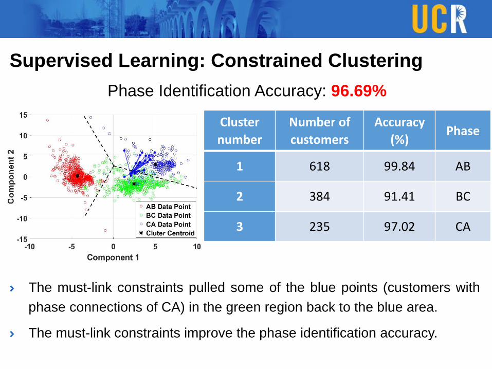
Supervised Learning: Constrained Clustering
Phase Identification Accuracy: 96.69%
The must-link constraints pulled some of the blue points (customers with
phase connections of CA) in the green region back to the blue area.
The must-link constraints improve the phase identification accuracy.
Cluster
number
Number of
customers
Accuracy
(%) Phase
1 618 99.84 AB
2 384 91.41 BC
3 235 97.02 CA

Visualization of Phase Identification Results
With GIS inputs, visualization of
distribution circuit with phase
connection information can be
generated automatically
Each line is colored
according to its actual phase
Each structure is
represented by a small dot
A colored rectangle is
overlaid on top of a structure
if it is assigned to the wrong
cluster.
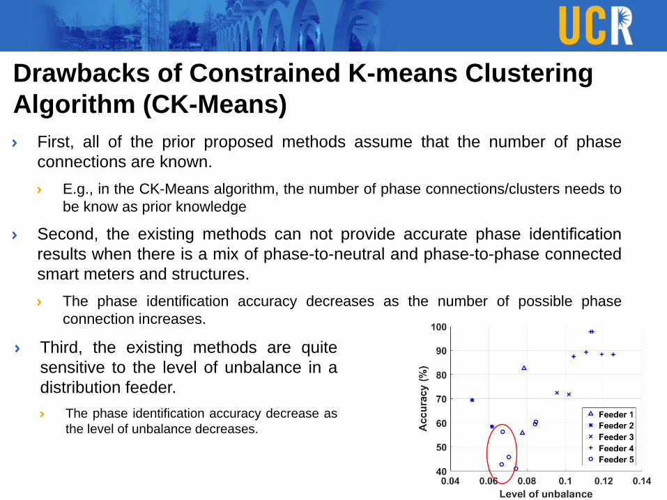
Drawbacks of Constrained K-means Clustering
Algorithm (CK-Means)
First, all of the prior proposed methods assume that the number of phase
connections are known.
E.g., in the CK-Means algorithm, the number of phase connections/clusters needs to
be know as prior knowledge
Second, the existing methods can not provide accurate phase identification
results when there is a mix of phase-to-neutral and phase-to-phase connected
smart meters and structures.
The phase identification accuracy decreases as the number of possible phase
connection increases.
Third, the existing methods are quite
sensitive to the level of unbalance in a
distribution feeder.
The phase identification accuracy decrease as
the level of unbalance decreases.
Phase Identification
Phase Connectivity Identification
Unsupervised Machine Learning
Linear dimension reduction and centroid-based clustering
Nonlinear dimension reduction and density-based clustering
Supervised Machine Learning
A comprehensive evaluation of supervised machine learning algorithms
Improvement with the theory of information losses

Nonlinear Dimension Reduction & Density-based
Clustering2
General Framework
2. W. Wang and N. Yu, "AMI Data Driven Phase Identification in Smart Grid," the Second International Conference on Green
Communications, Computing and Technologies, pp. 1-8, Rome, Italy, Sep. 2017.
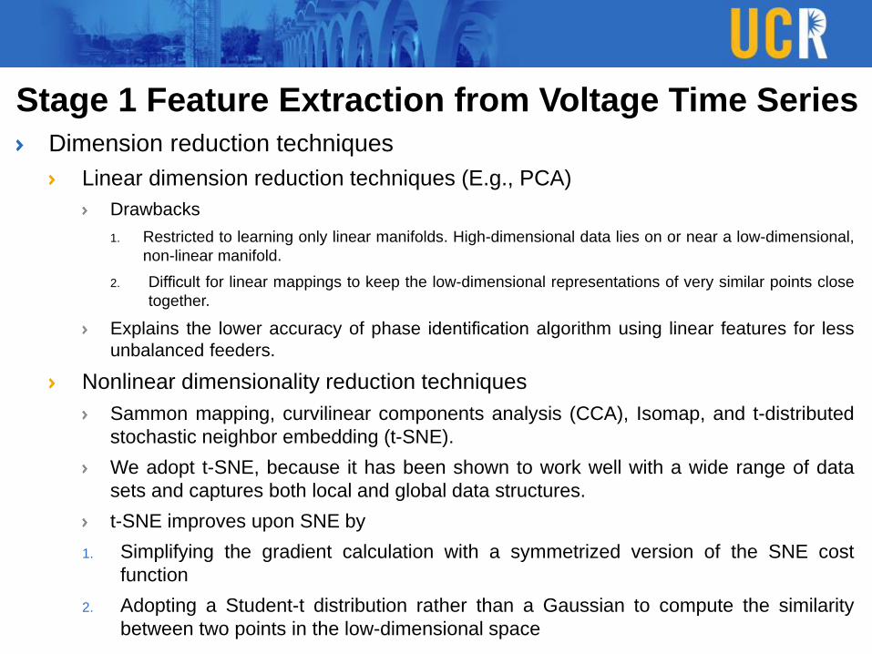
Stage 1 Feature Extraction from Voltage Time Series
Dimension reduction techniques
Linear dimension reduction techniques (E.g., PCA)
Drawbacks
1. Restricted to learning only linear manifolds. High-dimensional data lies on or near a low-dimensional,
non-linear manifold.
2. Difficult for linear mappings to keep the low-dimensional representations of very similar points close
together.
Explains the lower accuracy of phase identification algorithm using linear features for less
unbalanced feeders.
Nonlinear dimensionality reduction techniques
Sammon mapping, curvilinear components analysis (CCA), Isomap, and t-distributed
stochastic neighbor embedding (t-SNE).
We adopt t-SNE, because it has been shown to work well with a wide range of data
sets and captures both local and global data structures.
t-SNE improves upon SNE by
1. Simplifying the gradient calculation with a symmetrized version of the SNE cost
function
2. Adopting a Student-t distribution rather than a Gaussian to compute the similarity
between two points in the low-dimensional space

Comparison between PCA & t-SNE
The data points are not well
separated according to phase
connection with linear dimension
reduction.
The non-linear dimensionality reduction
technique does a much better job in extracting
hidden features from the voltage time series
during a less unbalanced period for the
feeders.
Feeder 5, data set 18 with a low level of unbalance

Phase Identification Accuracy with CK-Means and
the Proposed Method
The proposed phase identification algorithm significantly outperforms the
CK-Means method with all data sets in terms of accuracy.
On average, the proposed phase identification algorithm improves the
identification accuracy by 19.81% over the CK-Means algorithm.
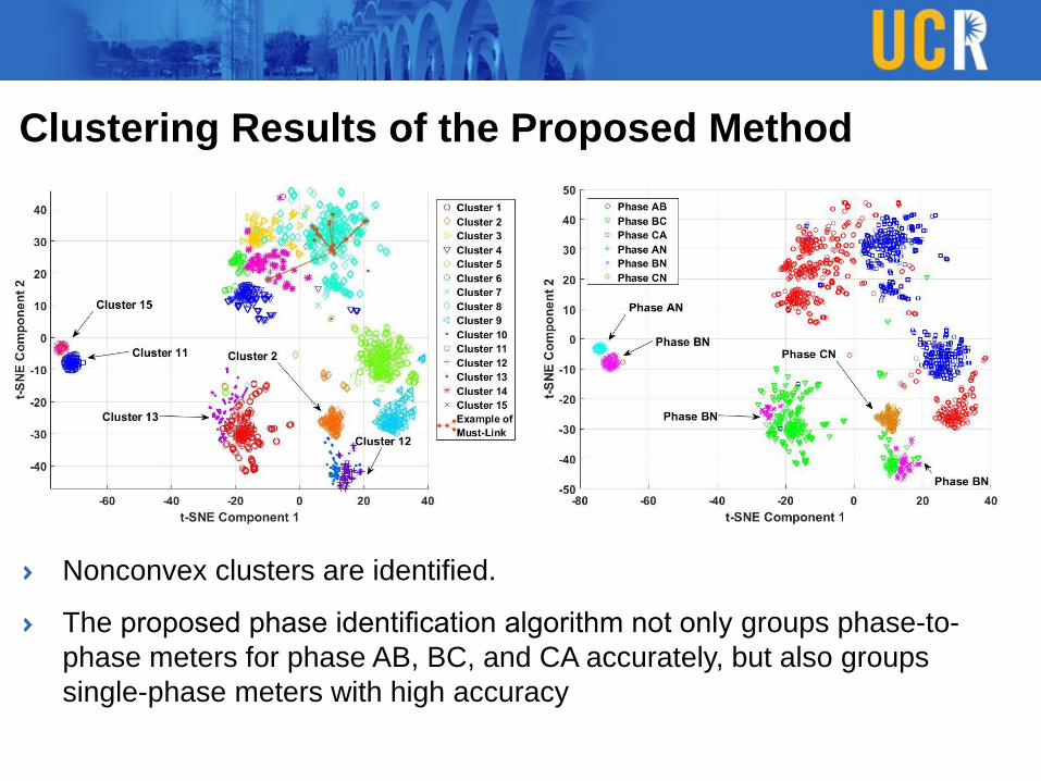
Clustering Results of the Proposed Method
Nonconvex clusters are identified.
The proposed phase identification algorithm not only groups phase-to-
phase meters for phase AB, BC, and CA accurately, but also groups
single-phase meters with high accuracy
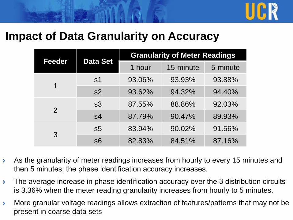
Impact of Data Granularity on Accuracy
As the granularity of meter readings increases from hourly to every 15 minutes and
then 5 minutes, the phase identification accuracy increases.
The average increase in phase identification accuracy over the 3 distribution circuits
is 3.36% when the meter reading granularity increases from hourly to 5 minutes.
More granular voltage readings allows extraction of features/patterns that may not be
present in coarse data sets
Feeder Data SetGranularity of Meter Readings
1 hour 15-minute 5-minute
1s1 93.06% 93.93% 93.88%
s2 93.62% 94.32% 94.40%
2s3 87.55% 88.86% 92.03%
s4 87.79% 90.47% 89.93%
3s5 83.94% 90.02% 91.56%
s6 82.83% 84.51% 87.16%

Phase Identification
Phase Connectivity Identification
Unsupervised Machine Learning
Linear dimension reduction and centroid-based clustering
Nonlinear dimension reduction and density-based clustering
Supervised Machine Learning
A comprehensive evaluation of supervised machine learning algorithms
Improvement with the theory of information losses

A Comprehensive Evaluation of Supervised
Machine Learning Algorithms
NN – Nearest Neighbor
DT – Decision Tree
RF – Random Forest
Ada – Adaboost
LR – Logistic Regression
ANN – Neural Network
MCD – Monte Carlo Dropout
Train% 5% 10% 20% 30%
1-NN 95.4% 95.7% 96.6% 96.7%
5-NN 93.1% 94.2% 95.7% 96.0%
DT 88.9% 92.0% 92.5% 94.4%
RF 92.4% 94.6% 96.0% 96.4%
Ada 89.5% 92.5% 94.1% 95.0%
LR 97.8% 98.0% 98.3% 98.2%
ANN 96.8% 98.3% 99.0% 99.0%
MCD 97.2% 98.7% 99.0% 99.0%
Simple Circuit Example

A Comprehensive Evaluation of Supervised
Machine Learning Algorithms
NN – Nearest Neighbor
DT – Decision Tree
RF – Random Forest
Ada – Adaboost
LR – Logistic Regression
ANN – Neural Network
MCD – Monte Carlo Dropout
Train% 5% 10% 20% 30%
1-NN 80.3% 84.1% 89.0% 92.0%
5-NN 78.0% 80.7% 83.5% 85.9%
DT 78.7% 81.5% 84.7% 87.1%
RF 83.2% 85.9% 88.6% 90.5%
Ada 78.6% 81.2% 84.1% 85.8%
LR 88.8% 90.3% 91.6% 91.9%
ANN 90.9% 93.2% 95.0% 96.7%
MCD 91.74% 93.6% 95.47% 96.5%
Complex Circuit Example
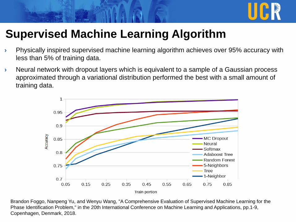
Supervised Machine Learning Algorithm
Physically inspired supervised machine learning algorithm achieves over 95% accuracy with
less than 5% of training data.
Neural network with dropout layers which is equivalent to a sample of a Gaussian process
approximated through a variational distribution performed the best with a small amount of
training data.
Brandon Foggo, Nanpeng Yu, and Wenyu Wang, "A Comprehensive Evaluation of Supervised Machine Learning for the
Phase Identification Problem," in the 20th International Conference on Machine Learning and Applications, pp.1-9,
Copenhagen, Denmark, 2018.

Training Data Selection
Not all data is equally useful.
Facility location optimization:
Feeder 5% random 5% selected
1 93.4% 97.9%
2 91.0% 95.3%
3 95.2% 96.7%
4 93.3% 97.2%
5 98.8% 99.6%
6 88.0% 91.9%
7 97.2% 98.6%
Training data selection
improves accuracies by
3% on average.
Phase Identification
Phase Connectivity Identification
Unsupervised Machine Learning
Linear dimension reduction and centroid-based clustering
Nonlinear dimension reduction and density-based clustering
Supervised Machine Learning
A comprehensive evaluation of supervised machine learning algorithms
Improvement with the theory of information losses
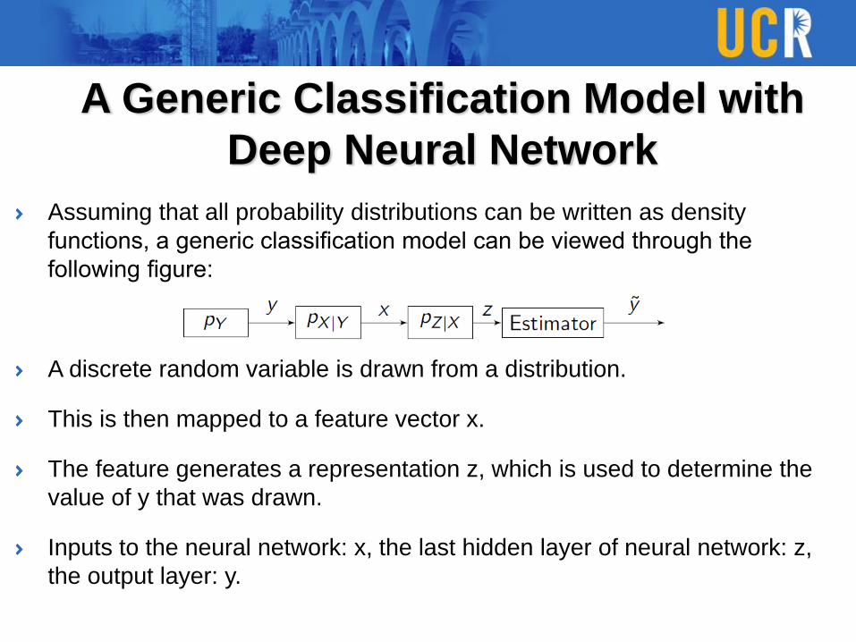
A Generic Classification Model with
Deep Neural Network
Assuming that all probability distributions can be written as density
functions, a generic classification model can be viewed through the
following figure:
A discrete random variable is drawn from a distribution.
This is then mapped to a feature vector x.
The feature generates a representation z, which is used to determine the
value of y that was drawn.
Inputs to the neural network: x, the last hidden layer of neural network: z,
the output layer: y.
Why is the Representation Important?
We could have just said that we have an estimator 𝑦 generated from the
feature vector x without explicit reference to the ‘inner’ variable z.
But z itself is an important variable to study.
‘Complicated’ representations tend to make the final estimation step harder.
e.g., if dim(𝑍) → ∞, we will need infinite training data to ‘cover’ the space.
But too simple a representation will lose its ability to estimate at all
e.g., if z = 0 ∀𝑦, then we can do better than random guessing.
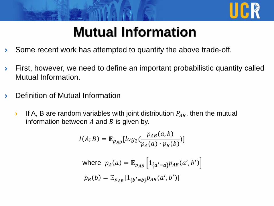
Mutual InformationSome recent work has attempted to quantify the above trade-off.
First, however, we need to define an important probabilistic quantity called
Mutual Information.
Definition of Mutual Information
If A, B are random variables with joint distribution 𝑃𝐴𝐵, then the mutual
information between 𝐴 and 𝐵 is given by.
𝐼 𝐴; 𝐵 = 𝔼𝑝𝐴𝐵[𝑙𝑜𝑔2(𝑝𝐴𝐵(𝑎, 𝑏)
𝑝𝐴(𝑎) ∙ 𝑝𝐵(𝑏))]
where 𝑝𝐴 𝑎 = 𝔼𝑝𝐴𝐵 1 𝑎′=𝑎 𝑝𝐴𝐵 𝑎′, 𝑏′
𝑝𝐵 𝑏 = 𝔼𝑝𝐴𝐵[1{𝑏′=𝑏}𝑝𝐴𝐵(𝑎′, 𝑏′)]
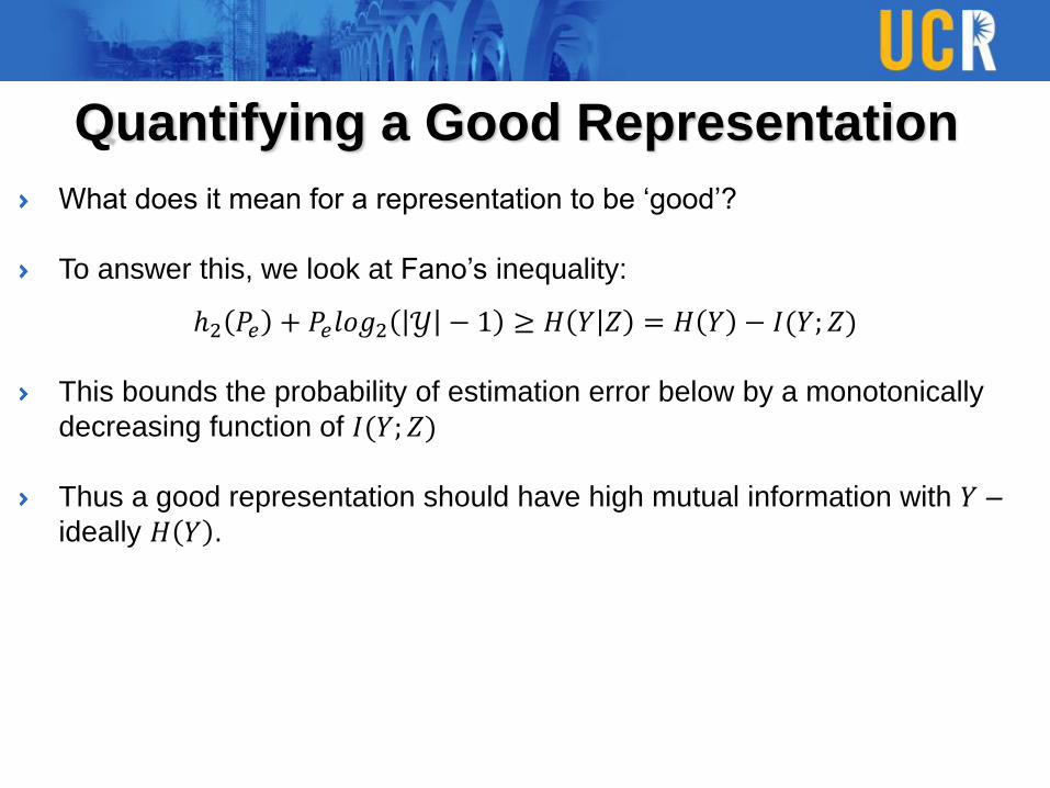
Quantifying a Good Representation
What does it mean for a representation to be ‘good’?
To answer this, we look at Fano’s inequality:
ℎ2 𝑃𝑒 + 𝑃𝑒𝑙𝑜𝑔2 𝒴 − 1 ≥ 𝐻 𝑌 𝑍 = 𝐻 𝑌 − 𝐼(𝑌; 𝑍)
This bounds the probability of estimation error below by a monotonically
decreasing function of 𝐼(𝑌; 𝑍)
Thus a good representation should have high mutual information with 𝑌 –
ideally 𝐻 𝑌 .

Finite Data Information Losses
But the representation can only retain as much information as it has seen
from the samples training it.
Thus full information of a random variable cannot be transfer to a
representation by finite samples – some information is lost.
We thus need to study these information losses.

Existing StudiesExisting literature has made some progress on such losses.
Letting መ𝐼(𝑌; 𝑍) refer to the information between 𝑌 and 𝑍 in a model
parameterized as 𝑝 𝑥 Ƹ𝑝 𝑦 𝑥 𝑝(𝑧|𝑥), we have:
𝐼 𝑌; 𝑍 − መ𝐼(𝑌; 𝑍) ≤ 𝒪(𝒴
2𝑚2𝐼(𝑋;𝑍))
This bound[1,2] leads to the idea of using 𝐼(𝑋; 𝑍) as a measure of complexity
of 𝑍 as, according to this bound, increasing 𝐼(𝑋; 𝑍) leads to gigantic losses!
But recent experimental work has shown that deep neural network models
have small losses even with high 𝐼 𝑋; 𝑍 - this bound is extremely lax.
1. Ravid Shwartz-Ziv and Naftali Tishby, Opening the black box of deep neural networks via information, arXiv
preprint arXiv:1703.00810 (2017).
2. Naftali Tishby and Noga Zaslavsky, Deep learning and the information bottleneck principle, Information Theory
Workshop (ITW), 2015 IEEE.
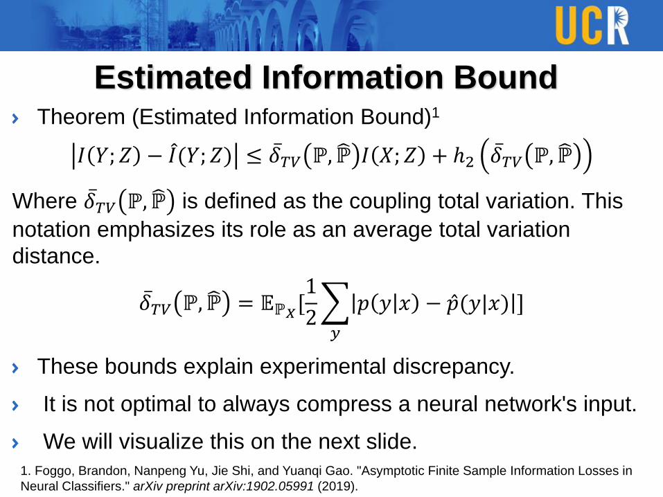
Estimated Information BoundTheorem (Estimated Information Bound)1
𝐼 𝑌; 𝑍 − መ𝐼(𝑌; 𝑍) ≤ ҧ𝛿𝑇𝑉 ℙ, ℙ 𝐼 𝑋; 𝑍 + ℎ2 ҧ𝛿𝑇𝑉 ℙ, ℙ
Where ҧ𝛿𝑇𝑉 ℙ, ℙ is defined as the coupling total variation. This
notation emphasizes its role as an average total variation
distance.
ҧ𝛿𝑇𝑉 ℙ, ℙ = 𝔼ℙ𝑋[1
2
𝑦
𝑝 𝑦 𝑥 − Ƹ𝑝(𝑦|𝑥) ]
These bounds explain experimental discrepancy.
It is not optimal to always compress a neural network's input.
We will visualize this on the next slide.
1. Foggo, Brandon, Nanpeng Yu, Jie Shi, and Yuanqi Gao. "Asymptotic Finite Sample Information Losses in
Neural Classifiers." arXiv preprint arXiv:1902.05991 (2019).
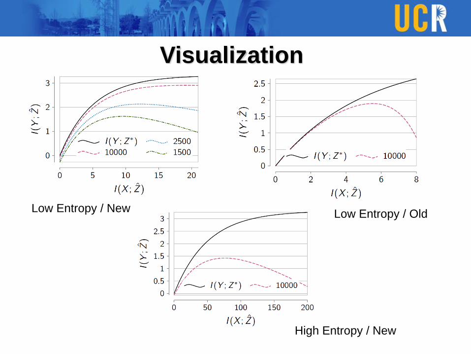
Visualization
Low Entropy / NewLow Entropy / Old
High Entropy / New

Information LoadingThe entropy of the feature space for phase identification
problem is very low1.
An information ‘anti-regularization’ term should be added to
the loss function of supervised machine learning algorithm to
penalize compression.
ℒ − 𝛽𝐼(𝑋; 𝑍), 𝛽 > 0
Circuit Neural NetworkInformation Load &
Training Data Selection
I 80.7% 91.0%
II 64.7% 96.3%
III 74.1% 93.1%
IV 75.0% 98.8%
V 51.7% 97.3%
1. Brandon Foggo and Nanpeng Yu, "Improving Supervised Phase Identification Through the Theory
of Information Losses, under review," 2019.

OutlineWhy do we focus on electric power distribution systems?
Big Data in Power Distribution Systems
Volume, Variety, Velocity, and Value
Applications of Machine Learning and Big Data Analytics in Power
Distribution Systems
Topology Identification – Phase Connectivity Identification
Anomaly Detection – Electricity Theft Detection
Reinforcement Learning based Control – Volt-VAR Control
Predictive Maintenance – Distribution Transformers
Estimation of Behind-the-meter Solar Generation
Anomaly Detection - Electricity Theft
Problem Definition
Energy Theft: The activity of reducing electricity bill by altering the electricity
consumption (physical / cyber)
Physical: Bypassing the smart meter, tamper electricity meters
Cyber: Hack into meters, communication network to change kWh readings
Why is it important? (Business Value)
According to Northeast Group, LLC, the world loses $89.3 billion annually to
electricity theft in 2015 (India $16.2 billion).
In the North America energy theft costs between 0.5% and 3.5% of annual
gross revenue.
B.C. Hydro estimates up to 3% of energy theft with 1500 ‘electrical diversions’
caught in 3 years. Center Point estimates energy theft is 1% to 2%.
Traditional detection methods rely on labor intensive inspections.

Existing Approaches
The existing data-driven methods can be categorized into
three groups based on the type of data available
Group 1: Smart Meter Data Not Available
Leverage ancillary information: Biannual electricity consumption and credit scores.
Machine Learning Model: SVM [Nagi 2010], Random Forest [Ramos 2011], Fuzzy Clustering
[Angelos 2011].
Group 2: Smart Meter Data & Theft Cases
Supervised Machine Learning Model: Extreme learning machine [Nizar 2008].
If transformer consumption data is also available, then nontechnical loss can be detected in
an area with multiclass SVM [Jokar 2016].
Group 3: Smart Meter Data, Network Topology & Topology Info
State-estimation based approaches [Huang 2013].
Formulate anomaly detection as an optimization problem [Drzajic 2015].

Drawbacks of the Existing Approaches
Most electric utilities cannot obtain the data necessary to use
them
Transformer data, reliable topology documentation, and network
parameter information are not readily available.
Many existing methods analyze electricity consumption data
alone
These methods cannot distinguish electricity theft from non-malicious
customer activities. (Installation of a new electric device).
Supervised approaches for electricity theft detection need theft
samples.
Confirmed electricity theft cases are very rare.
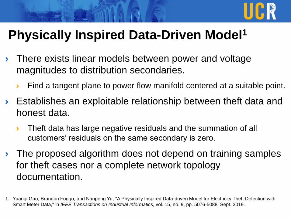
Physically Inspired Data-Driven Model1
There exists linear models between power and voltage
magnitudes to distribution secondaries.
Find a tangent plane to power flow manifold centered at a suitable point.
Establishes an exploitable relationship between theft data and
honest data.
Theft data has large negative residuals and the summation of all
customers’ residuals on the same secondary is zero.
The proposed algorithm does not depend on training samples
for theft cases nor a complete network topology
documentation.
1. Yuanqi Gao, Brandon Foggo, and Nanpeng Yu, "A Physically Inspired Data-driven Model for Electricity Theft Detection with
Smart Meter Data," in IEEE Transactions on Industrial Informatics, vol. 15, no. 9, pp. 5076-5088, Sept. 2019.
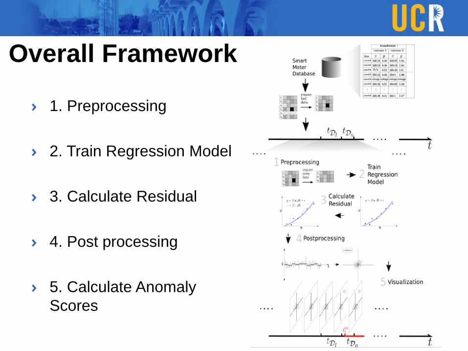
Overall Framework
1. Preprocessing
2. Train Regression Model
3. Calculate Residual
4. Post processing
5. Calculate Anomaly
Scores
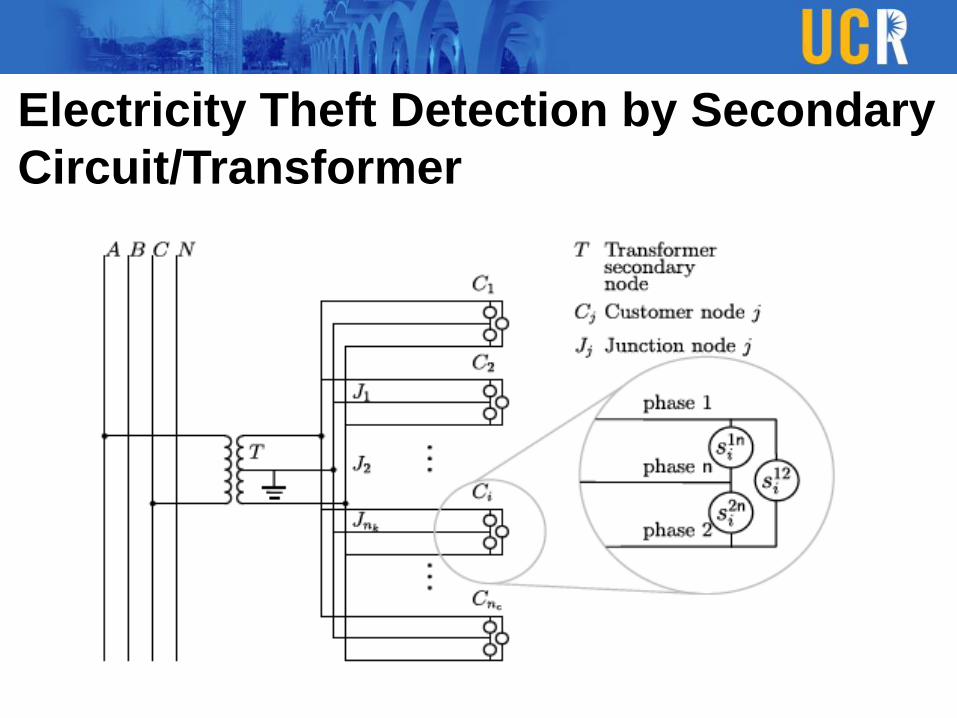
Electricity Theft Detection by Secondary
Circuit/Transformer

Linearized Power Flow Equations for
Unbalanced Secondary
𝐺11 −𝐺12
−𝐺12 𝐺22−𝐵11 𝐵12
𝐵21 −𝐵22
−𝐵11 𝐵12
𝐵21 𝐵22−𝐺11 𝐺12
𝐺21 −𝐺22
𝑣1
𝑣2
𝜃1
𝜃2
=
𝑝1
𝑝2
𝑞1
𝑞2
𝑝1, 𝑝2, 𝑞1, 𝑞2: Real and
Reactive Power injections
for phase 1 and 2
𝑣1, 𝑣2, 𝜃1, 𝜃2: Voltage
magnitude and angles for
phase 1 and 2
𝒚𝒓 =𝒑𝒓
𝒒𝒓=
𝑳𝟏𝟏𝒓 𝑳𝟏𝟐
𝒓
𝑳𝟐𝟏𝒓 𝑳𝟐𝟐
𝒓𝒗𝒓
𝜽𝒓= 𝑳𝒓𝒙𝒓
Approximate the nonlinear power flow equation as a linear one
ℱ 𝒗, 𝜽, 𝒑, 𝒒 = 𝟎 → Ϝഥ𝕏[𝒗𝑻, 𝜽𝑻, 𝒑𝑻, 𝒒𝑻]𝑻= 𝟎
Where Ϝഥ𝕏 is the Jacobian matrix of ℱ evaluated at some operating point ഥ𝕏 = [ ҧ𝑣 ҧ𝜃 ҧ𝑝 ത𝑞]𝑇 .This point must be itself be a solution to the power flow equation ℱ ഥ𝕏 = 0.
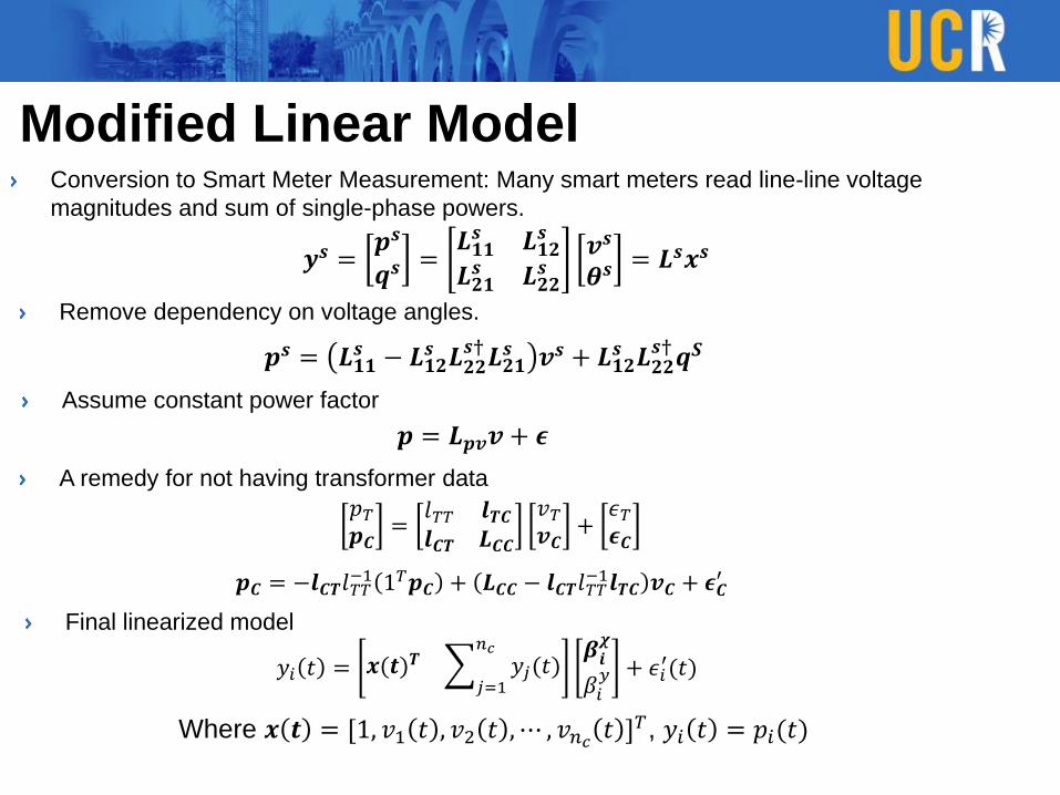
Modified Linear ModelConversion to Smart Meter Measurement: Many smart meters read line-line voltage
magnitudes and sum of single-phase powers.
𝒚𝒔 =𝒑𝒔
𝒒𝒔=
𝑳𝟏𝟏𝒔 𝑳𝟏𝟐
𝒔
𝑳𝟐𝟏𝒔 𝑳𝟐𝟐
𝒔𝒗𝒔
𝜽𝒔= 𝑳𝒔𝒙𝒔
Remove dependency on voltage angles.
𝒑𝒔 = 𝑳𝟏𝟏𝒔 − 𝑳𝟏𝟐
𝒔 𝑳𝟐𝟐𝒔†𝑳𝟐𝟏
𝒔 𝒗𝒔 + 𝑳𝟏𝟐𝒔 𝑳𝟐𝟐
𝒔†𝒒𝑺
Assume constant power factor
𝒑 = 𝑳𝒑𝒗𝒗 + 𝝐
A remedy for not having transformer data
𝑝𝑇𝒑𝑪
=𝑙𝑇𝑇 𝒍𝑻𝑪𝒍𝑪𝑻 𝑳𝑪𝑪
𝑣𝑇𝒗𝑪
+𝜖𝑇𝝐𝑪
𝒑𝑪 = −𝒍𝑪𝑻𝑙𝑇𝑇−1 1𝑇𝒑𝑪 + 𝑳𝑪𝑪 − 𝒍𝑪𝑻𝑙𝑇𝑇
−1𝒍𝑻𝑪 𝒗𝑪 + 𝝐𝑪′
Final linearized model
𝑦𝑖 𝑡 = 𝒙(𝒕)𝑻 𝑗=1
𝑛𝑐𝑦𝑗(𝑡)
𝜷𝒊𝝌
𝛽𝑖𝑦 + 𝜖𝑖
′(𝑡)
Where 𝒙 𝒕 = [1, 𝑣1 𝑡 , 𝑣2 𝑡 ,⋯ , 𝑣𝑛𝑐 𝑡 ]𝑇, 𝑦𝑖 𝑡 = 𝑝𝑖(𝑡)
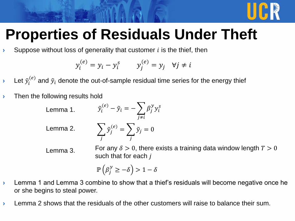
Properties of Residuals Under TheftSuppose without loss of generality that customer 𝑖 is the thief, then
𝑦𝑖(𝑒)
= 𝑦𝑖 − 𝑦𝑖𝑠 𝑦𝑗
(𝑒)= 𝑦𝑗 ∀𝑗 ≠ 𝑖
Let 𝑦𝑖(𝑒)
and 𝑦𝑖 denote the out-of-sample residual time series for the energy thief
Then the following results hold
𝑦𝑖(𝑒)
− 𝑦𝑖 = −
𝑗≠𝑖
𝛽𝑗𝑦𝑦𝑖𝑠
Lemma 1.
Lemma 2.
𝑗
𝑦𝑗(𝑒)
=
𝑗
𝑦𝑗 = 0
Lemma 3. For any 𝛿 > 0, there exists a training data window length 𝑇 > 0such that for each 𝑗
ℙ 𝛽𝑗𝑦≥ −𝛿 > 1 − 𝛿
Lemma 1 and Lemma 3 combine to show that a thief’s residuals will become negative once he
or she begins to steal power.
Lemma 2 shows that the residuals of the other customers will raise to balance their sum.

Anomaly Score & Energy Theft Detection
We define an anomaly score in terms of the residuals 𝑦𝑖 for each
customer 𝑖 and each rolling window 𝑓.
Customer and rolling window with higher anomaly scores are more likely
to be thieves or have malfunctioning smart meters.
Anomaly score 𝑑𝑖 𝑓 = 𝜔𝑖(𝑓) 𝑦𝑖′2 where 𝜔𝑖 𝑓 = 𝑡𝐷(𝑓) / 𝑦𝑖
𝐷(𝑓)2
is a
weighting coefficient.
Energy thefts are identified by ranking 𝑑𝑖 𝑓 for all 𝑖 and all 𝑓.
The higher 𝑑𝑖(𝑓) is the higher priority of investigation customer 𝑖 should
have.
This ranking method can be simplified to ranking 𝑚𝑎𝑥𝑓𝑑𝑖(𝑓) for all 𝑖 when
theft time is unimportant.
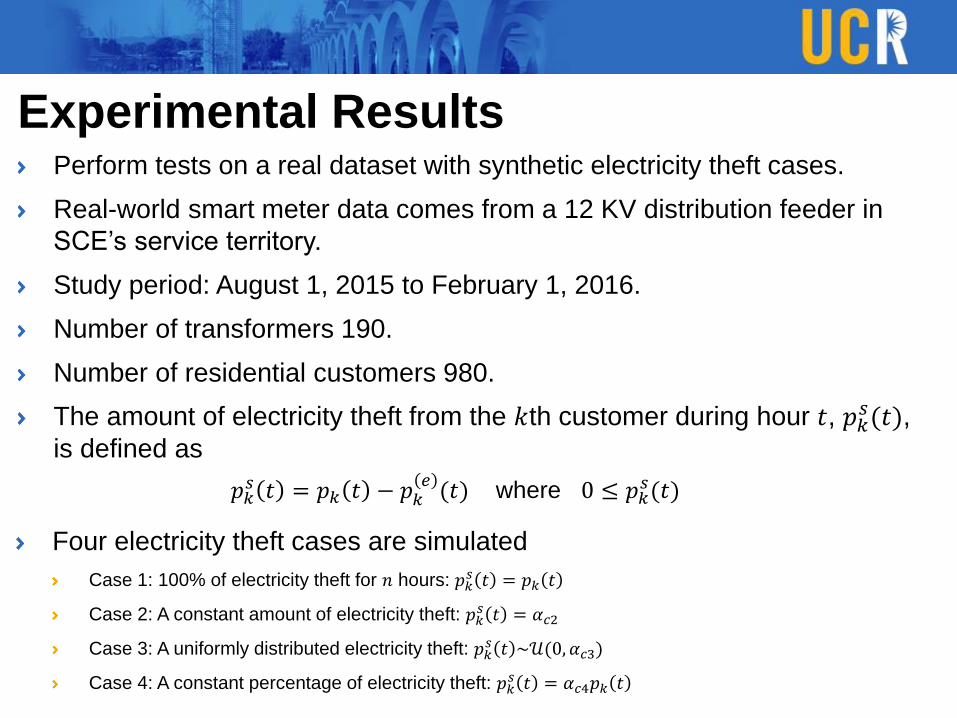
Perform tests on a real dataset with synthetic electricity theft cases.
Real-world smart meter data comes from a 12 KV distribution feeder in
SCE’s service territory.
Study period: August 1, 2015 to February 1, 2016.
Number of transformers 190.
Number of residential customers 980.
The amount of electricity theft from the 𝑘th customer during hour 𝑡, 𝑝𝑘𝑠(𝑡),
is defined as
Experimental Results
𝑝𝑘𝑠 𝑡 = 𝑝𝑘 𝑡 − 𝑝𝑘
𝑒(𝑡) where 0 ≤ 𝑝𝑘
𝑠(𝑡)
Four electricity theft cases are simulated
Case 1: 100% of electricity theft for 𝑛 hours: 𝑝𝑘𝑠 𝑡 = 𝑝𝑘 𝑡
Case 2: A constant amount of electricity theft: 𝑝𝑘𝑠 𝑡 = 𝛼𝑐2
Case 3: A uniformly distributed electricity theft: 𝑝𝑘𝑠 𝑡 ~𝒰(0, 𝛼𝑐3)
Case 4: A constant percentage of electricity theft: 𝑝𝑘𝑠 𝑡 = 𝛼𝑐4𝑝𝑘 𝑡
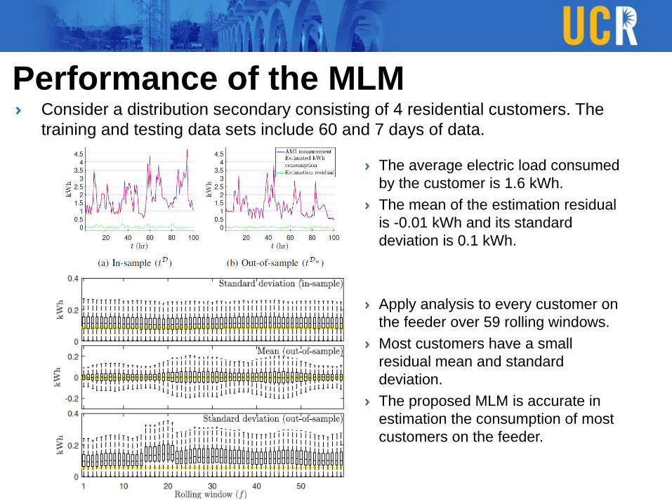
Performance of the MLMConsider a distribution secondary consisting of 4 residential customers. The
training and testing data sets include 60 and 7 days of data.
The average electric load consumed
by the customer is 1.6 kWh.
The mean of the estimation residual
is -0.01 kWh and its standard
deviation is 0.1 kWh.
Apply analysis to every customer on
the feeder over 59 rolling windows.
Most customers have a small
residual mean and standard
deviation.
The proposed MLM is accurate in
estimation the consumption of most
customers on the feeder.
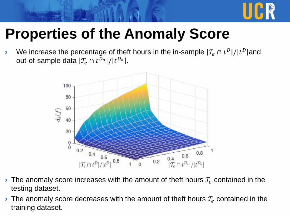
Properties of the Anomaly ScoreWe increase the percentage of theft hours in the in-sample 𝒯𝑒 ∩ 𝑡𝐷 / 𝑡𝐷 and
out-of-sample data 𝒯𝑒 ∩ 𝑡𝐷𝑎 / 𝑡𝐷𝑎 .
The anomaly score increases with the amount of theft hours 𝒯𝑒 contained in the
testing dataset.
The anomaly score decreases with the amount of theft hours 𝒯𝑒 contained in the
training dataset.

The Impact of Energy Theft on Out-of-
Sample ResidualsSynthesize smart meter data for customer 𝑘 under theft case 3.
We assume that the electricity theft activities occur from hour 𝑡1𝑒 = 25 to hour 𝑡2
𝑒 = 168 in the out-
of-sample period.
The amount of electricity theft follows a uniform distribution with 𝑝𝑘𝑠 𝑡 ~𝒰(0,1.8) kWh
Customer 𝑘 has negative residuals while the honest customers have positive residuals.
The sum of the residuals at any given hour is zero.
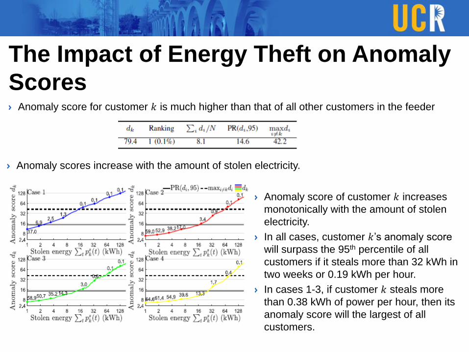
The Impact of Energy Theft on Anomaly
ScoresAnomaly score for customer 𝑘 is much higher than that of all other customers in the feeder
Anomaly scores increase with the amount of stolen electricity.
Anomaly score of customer 𝑘 increases
monotonically with the amount of stolen
electricity.
In all cases, customer 𝑘’s anomaly score
will surpass the 95th percentile of all
customers if it steals more than 32 kWh in
two weeks or 0.19 kWh per hour.
In cases 1-3, if customer 𝑘 steals more
than 0.38 kWh of power per hour, then its
anomaly score will the largest of all
customers.
OutlineWhy do we focus on electric power distribution systems?
Big Data in Power Distribution Systems
Volume, Variety, Velocity, and Value
Applications of Machine Learning and Big Data Analytics in Power
Distribution Systems
Topology Identification – Phase Connectivity Identification
Anomaly Detection – Electricity Theft Detection
Reinforcement Learning based Control – Volt-VAR Control
Predictive Maintenance – Distribution Transformers
Estimation of Behind-the-meter Solar Generation
MotivationPhysical Model-based Control in Power Distribution Systems
Advantages: theoretical guarantees in some cases.
Rely heavily on accurate knowledge of grid topology and parameters.
Unsatisfactory performance (e.g., VVC)
Practical Challenges
Difficult for regional utilities to maintain reliable network models oftentimes
involving millions of buses.
Secondary feeder (transfer-to-customer association, phase connectivity)
Reinforcement Learning-based (Model-free) Approach
Do not need reliable and complete distribution network model
Use operational data (real-time and/or historical)
Learn control policies by interacting with the distribution network.
Challenges: safe, optimality, sample efficient, robust.

Background of Volt-VAR Control (VVC)As penetration level of DERs continues to rise, it is increasingly difficult to
keep the nodal voltages within the desired range.
The voltage profile highly impacts the electricity service quality for end
users.
Over- and under-voltage reduce energy efficiency, cause equipment
malfunction, and damage customers’ electrical appliance.
Control objectives of VVC
Maintain voltages within allowable range
Manage power factor
Reduce network losses and equipment wear and tear.
Coordinate the operations of various voltage regulating devices
Voltage regulators, on-load tap changers
Switchable capacitor banks and smart inverters
Reinforcement Learning based ControlMain Idea
A computational approach to understanding and automating goal-directed
learning and decision making.
Key Difference (compare to other computational approaches)
Learning by an agent from direct interaction with its environment
Without requiring exemplary supervision or complete models of the environment.
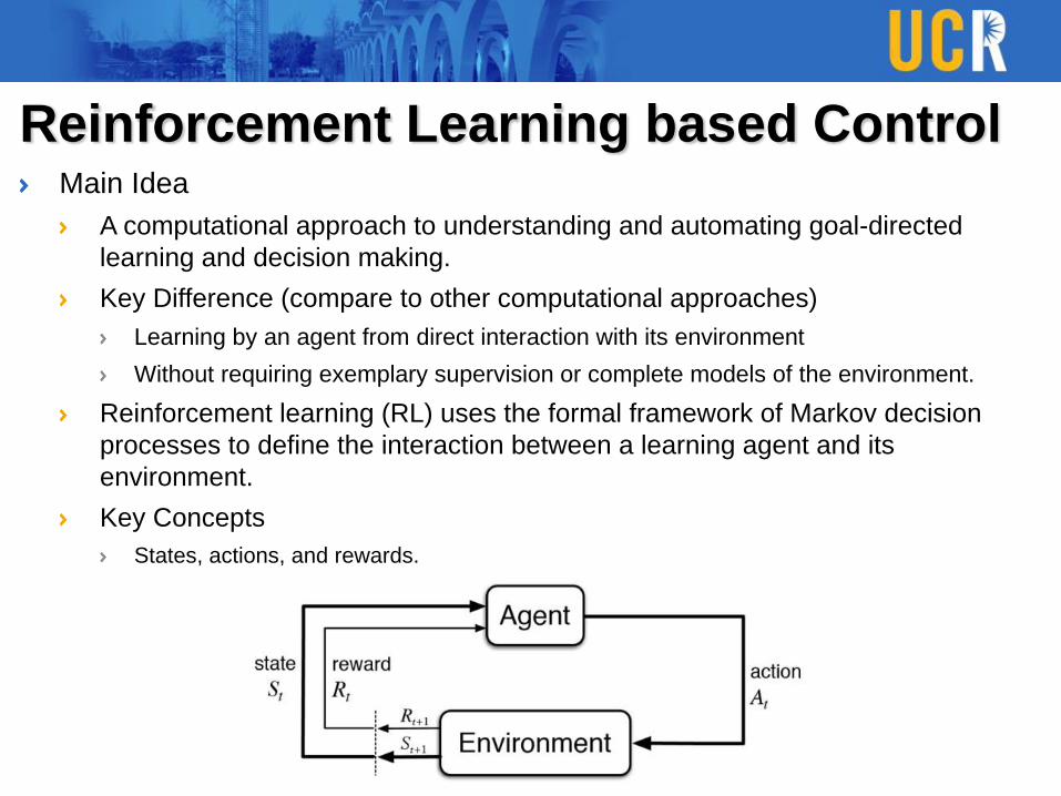
Reinforcement learning (RL) uses the formal framework of Markov decision
processes to define the interaction between a learning agent and its
environment.
Key Concepts
States, actions, and rewards.
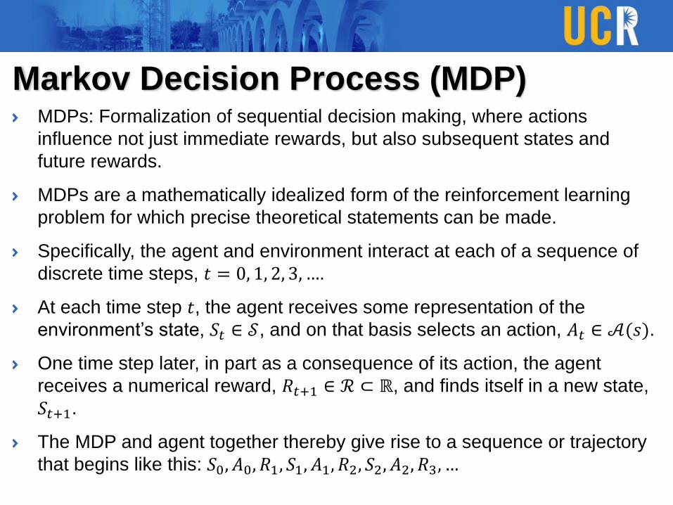
Markov Decision Process (MDP)MDPs: Formalization of sequential decision making, where actions
influence not just immediate rewards, but also subsequent states and
future rewards.
MDPs are a mathematically idealized form of the reinforcement learning
problem for which precise theoretical statements can be made.
Specifically, the agent and environment interact at each of a sequence of
discrete time steps, 𝑡 = 0, 1, 2, 3, ….
At each time step 𝑡, the agent receives some representation of the
environment’s state, 𝑆𝑡 ∈ 𝒮, and on that basis selects an action, 𝐴𝑡 ∈ 𝒜(𝑠).
One time step later, in part as a consequence of its action, the agent
receives a numerical reward, 𝑅𝑡+1 ∈ ℛ ⊂ ℝ, and finds itself in a new state,
𝑆𝑡+1.
The MDP and agent together thereby give rise to a sequence or trajectory
that begins like this: 𝑆0, 𝐴0, 𝑅1, 𝑆1, 𝐴1, 𝑅2, 𝑆2, 𝐴2, 𝑅3, …
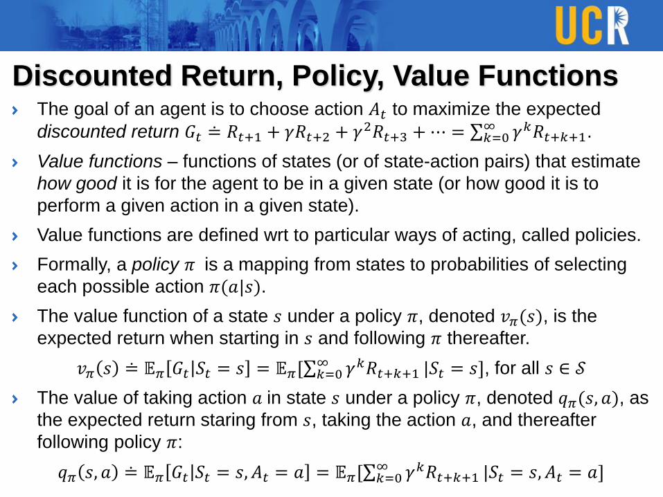
Discounted Return, Policy, Value FunctionsThe goal of an agent is to choose action 𝐴𝑡 to maximize the expected
discounted return 𝐺𝑡 ≐ 𝑅𝑡+1 + 𝛾𝑅𝑡+2 + 𝛾2𝑅𝑡+3 +⋯ = σ𝑘=0∞ 𝛾𝑘𝑅𝑡+𝑘+1.
Value functions – functions of states (or of state-action pairs) that estimate
how good it is for the agent to be in a given state (or how good it is to
perform a given action in a given state).
Value functions are defined wrt to particular ways of acting, called policies.
Formally, a policy 𝜋 is a mapping from states to probabilities of selecting
each possible action 𝜋(𝑎|𝑠).
The value function of a state 𝑠 under a policy 𝜋, denoted 𝑣𝜋(𝑠), is the
expected return when starting in 𝑠 and following 𝜋 thereafter.
𝑣𝜋 𝑠 ≐ 𝔼𝜋 𝐺𝑡 𝑆𝑡 = 𝑠 = 𝔼𝜋[σ𝑘=0∞ 𝛾𝑘𝑅𝑡+𝑘+1 |𝑆𝑡 = 𝑠], for all 𝑠 ∈ 𝒮
The value of taking action 𝑎 in state 𝑠 under a policy 𝜋, denoted 𝑞𝜋(𝑠, 𝑎), as
the expected return staring from 𝑠, taking the action 𝑎, and thereafter
following policy 𝜋:
𝑞𝜋 𝑠, 𝑎 ≐ 𝔼𝜋 𝐺𝑡 𝑆𝑡 = 𝑠, 𝐴𝑡 = 𝑎 = 𝔼𝜋[σ𝑘=0∞ 𝛾𝑘𝑅𝑡+𝑘+1 |𝑆𝑡 = 𝑠, 𝐴𝑡 = 𝑎]
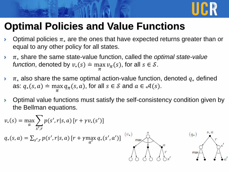
Optimal Policies and Value FunctionsOptimal policies 𝜋∗ are the ones that have expected returns greater than or
equal to any other policy for all states.
𝜋∗ share the same state-value function, called the optimal state-value
function, denoted by 𝑣∗(𝑠) ≐ max𝜋
𝑣𝜋(𝑠), for all 𝑠 ∈ 𝒮.
𝜋∗ also share the same optimal action-value function, denoted 𝑞∗ defined
as: 𝑞∗(𝑠, 𝑎) ≐ max𝜋
𝑞𝜋(𝑠, 𝑎), for all 𝑠 ∈ 𝒮 and 𝑎 ∈ 𝒜(𝑠).
Optimal value functions must satisfy the self-consistency condition given by
the Bellman equations.
𝑣∗ 𝑠 = max𝑎
𝑠′,𝑟
𝑝(𝑠′, 𝑟|𝑠, 𝑎) [𝑟 + 𝛾𝑣∗(𝑠′)]
𝑞∗(𝑠, 𝑎) = σ𝑠′,𝑟 𝑝(𝑠′, 𝑟|𝑠, 𝑎) [𝑟 + 𝛾max
𝑎′𝑞∗(𝑠
′, 𝑎′)]
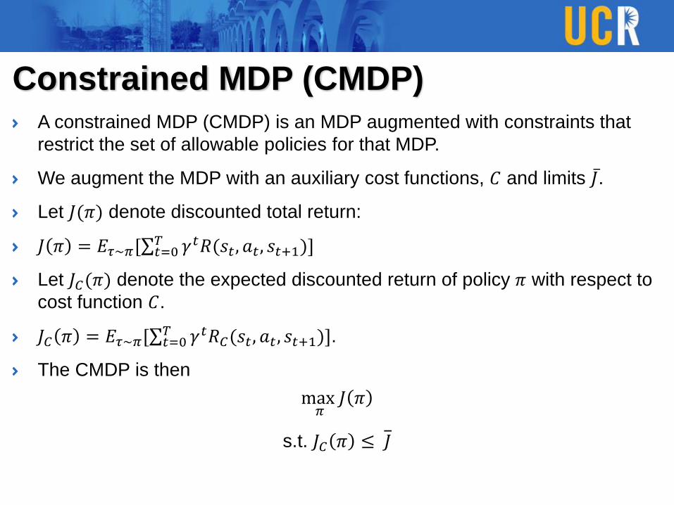
Constrained MDP (CMDP)A constrained MDP (CMDP) is an MDP augmented with constraints that
restrict the set of allowable policies for that MDP.
We augment the MDP with an auxiliary cost functions, 𝐶 and limits ҧ𝐽.
Let 𝐽(𝜋) denote discounted total return:
𝐽 𝜋 = 𝐸𝜏∼𝜋[σ𝑡=0𝑇 𝛾𝑡𝑅(𝑠𝑡, 𝑎𝑡, 𝑠𝑡+1)]
Let 𝐽𝐶(𝜋) denote the expected discounted return of policy 𝜋 with respect to
cost function 𝐶.
𝐽𝐶 𝜋 = 𝐸𝜏∼𝜋[σ𝑡=0𝑇 𝛾𝑡𝑅𝐶(𝑠𝑡, 𝑎𝑡, 𝑠𝑡+1)].
The CMDP is then
max𝜋
𝐽 𝜋
s.t. 𝐽𝐶 𝜋 ≤ 𝐽
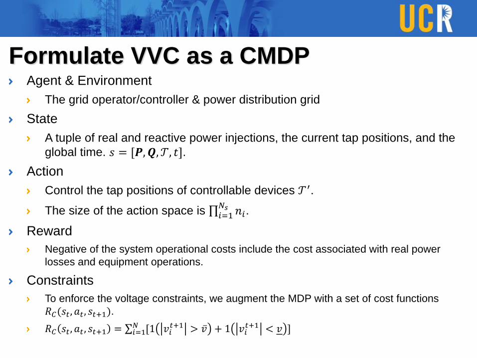
Formulate VVC as a CMDPAgent & Environment
The grid operator/controller & power distribution grid
State
A tuple of real and reactive power injections, the current tap positions, and the
global time. 𝑠 = [𝑷,𝑸, 𝒯, 𝑡].
Action
Control the tap positions of controllable devices 𝒯′.
The size of the action space is ς𝑖=1𝑁𝑠 𝑛𝑖.
Reward
Negative of the system operational costs include the cost associated with real power
losses and equipment operations.
Constraints
To enforce the voltage constraints, we augment the MDP with a set of cost functions
𝑅𝐶(𝑠𝑡, 𝑎𝑡, 𝑠𝑡+1).
𝑅𝐶 𝑠𝑡, 𝑎𝑡, 𝑠𝑡+1 = σ𝑖=1𝑁 [1 𝑣𝑖
𝑡+1 > ҧ𝑣 + 1 𝑣𝑖𝑡+1 < 𝑣 ]

Policy Gradient MethodAction-value Methods
Approximate the action-value functions through learning and then selects
actions based on estimated action-value functions.
Policy Gradient Methods (PGM)
Learn a parameterized control policy that directly selects actions without
consulting a value function.
Advantages of PGM
The policy function could be easier to approximate than the action-value
functions.
The parameterized policy could be more smooth and flexible than the 𝜖-greedy
choice.
Policy Gradient Theorem
𝛻𝐽 𝜋𝜃 = 𝐸𝜏∼𝜋𝜃
𝑡=0
𝑇
𝛻𝜃𝑙𝑛 𝜋𝜃 𝑎𝑡 𝑠𝑡 𝐺𝑡 − 𝑏 𝑠𝑡 = 𝐸𝜏∼𝜋𝜃 [
𝑡=0
𝑇
𝛻𝜃𝑙𝑛 𝜋𝜃 𝑎𝑡 𝑠𝑡 (𝑄𝜋𝜃 𝑠𝑡 , 𝑎𝑡 − 𝑏 𝑠𝑡 )]
𝐺𝑡: discounted return. 𝑏(𝑠𝑡): baseline function, which helps reduce variance.
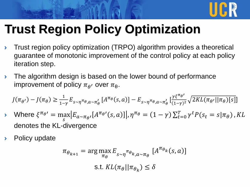
Trust Region Policy Optimization
Trust region policy optimization (TRPO) algorithm provides a theoretical
guarantee of monotonic improvement of the control policy at each policy
iteration step.
The algorithm design is based on the lower bound of performance
improvement of policy 𝜋𝜃′ over 𝜋θ.
𝐽 𝜋𝜃′ − 𝐽 𝜋𝜃 ≥1
1−𝛾𝐸𝑠∼𝜂𝜋𝜃 ,𝑎∼𝜋𝜃
′ [𝐴𝜋𝜃 𝑠, 𝑎 ] − 𝐸𝑠∼𝜂𝜋𝜃 ,𝑎∼𝜋𝜃′ [
𝛾𝜉𝜋𝜃′
1−𝛾 2 2𝐾𝐿(𝜋𝜃′||𝜋𝜃)[𝑠]]
Where 𝜉𝜋𝜃′ = max𝑠
𝐸𝑎∼𝜋𝜃′ 𝐴𝜋𝜃′ 𝑠, 𝑎 , 𝜂𝜋𝜃 = 1 − 𝛾 σ𝑡=0
𝑇 𝛾𝑡𝑃(𝑠𝑡 = 𝑠|𝜋𝜃) , 𝐾𝐿
denotes the KL-divergence
Policy update
𝜋𝜃𝑘+1 = argmax𝜋𝜃
𝐸𝑠∼𝜂
𝜋𝜃𝑘 ,𝑎∼𝜋𝜃[𝐴𝜋𝜃𝑘 𝑠, 𝑎 ]
s.t. 𝐾𝐿(𝜋𝜃||𝜋𝜃𝑘) ≤ 𝛿
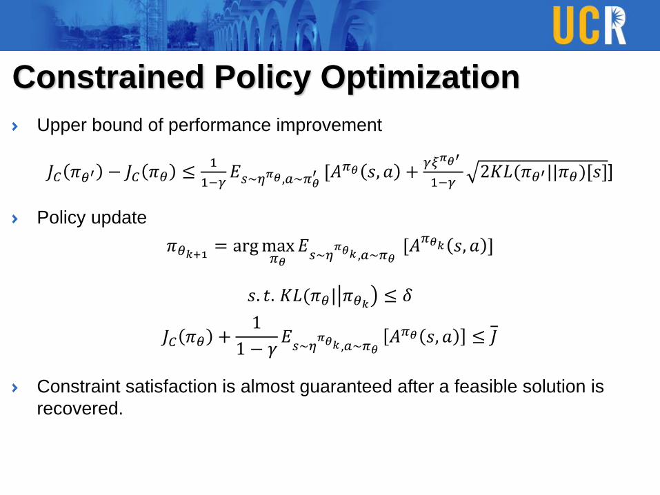
Constrained Policy Optimization
Upper bound of performance improvement
𝐽𝐶 𝜋𝜃′ − 𝐽𝐶 𝜋𝜃 ≤1
1−𝛾𝐸𝑠∼𝜂𝜋𝜃 ,𝑎∼𝜋𝜃
′ [𝐴𝜋𝜃 𝑠, 𝑎 +𝛾𝜉𝜋𝜃′
1−𝛾2𝐾𝐿(𝜋𝜃′||𝜋𝜃)[𝑠]]
Policy update
𝜋𝜃𝑘+1 = argmax𝜋𝜃
𝐸𝑠∼𝜂
𝜋𝜃𝑘 ,𝑎∼𝜋𝜃[𝐴𝜋𝜃𝑘 𝑠, 𝑎 ]
𝑠. 𝑡. 𝐾𝐿(𝜋𝜃| 𝜋𝜃𝑘 ≤ 𝛿
𝐽𝐶 𝜋𝜃 +1
1 − 𝛾𝐸𝑠∼𝜂
𝜋𝜃𝑘 ,𝑎∼𝜋𝜃𝐴𝜋𝜃 𝑠, 𝑎 ≤ 𝐽
Constraint satisfaction is almost guaranteed after a feasible solution is
recovered.

Numerical StudyTest Systems
IEEE 4-bus and 13-bus distribution test feeders.
Nodal Load and Voltage Measurements
Aggregated real-world smart meter data. Nodal voltages calculated via power
flow simulations.
Length of training data: 6 months. Length of test data: 1 week.
Switching Devices
Each test feeder has three switching devices: a voltage regulator, an on-load
tap changer, and a capacitor bank.
Both the voltage regulator and on-load tap changer have 11 tap positions with
turns ratios between 0.95 and 1.05.
The number of tap positions of the capacitor bank is treated to be 2.
The size of the action space for each test case is 242.
Electricity price: $40/MWh. Switching costs: $0.1 per tap change.

Benchmarking & Performance Comparison
The MPC-based optimization algorithm is chosen as the first benchmark.
Control horizon: 24 hours.
The ARIMA model is used to forecast the load during the control horizon.
The mixed integer conic programming problem (MICP) is solved on a rolling basis.
MOSEK and GUROBI are used to solve the MICP problem.
The second benchmark is set up by replacing the load forecast with actual
load data in the MPC framework.
The last benchmark represents the baseline where all switching devices
are kept at their initial positions.
CPO algorithm
outperform the
TRPO algorithm by
achieving a higher
average
discounted return.
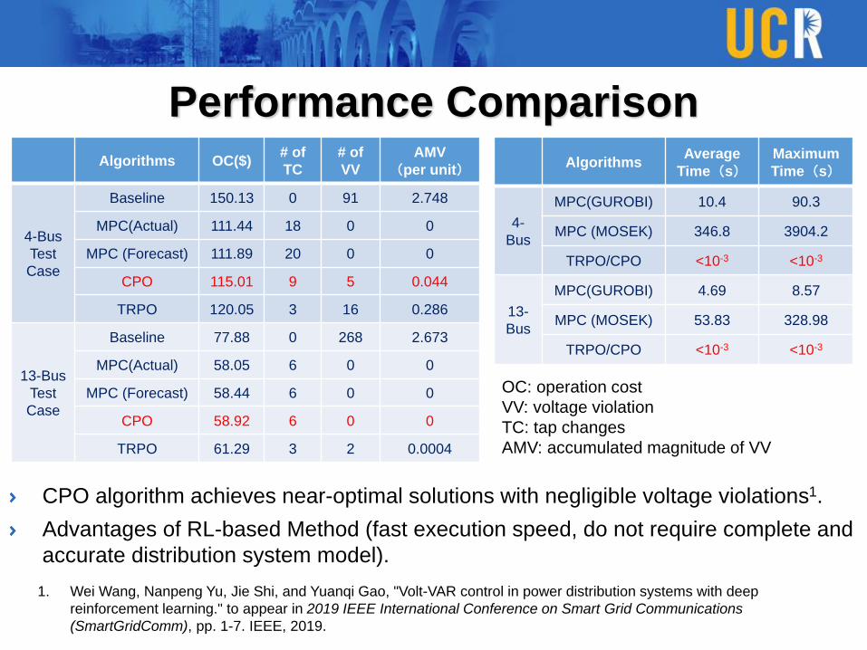
Performance Comparison
CPO algorithm achieves near-optimal solutions with negligible voltage violations1.
Advantages of RL-based Method (fast execution speed, do not require complete and
accurate distribution system model).
Algorithms OC($)# of
TC
# of
VV
AMV
(per unit)
4-Bus
Test
Case
Baseline 150.13 0 91 2.748
MPC(Actual) 111.44 18 0 0
MPC (Forecast) 111.89 20 0 0
CPO 115.01 9 5 0.044
TRPO 120.05 3 16 0.286
13-Bus
Test
Case
Baseline 77.88 0 268 2.673
MPC(Actual) 58.05 6 0 0
MPC (Forecast) 58.44 6 0 0
CPO 58.92 6 0 0
TRPO 61.29 3 2 0.0004
OC: operation cost
VV: voltage violation
TC: tap changes
AMV: accumulated magnitude of VV
AlgorithmsAverage
Time(s)Maximum
Time(s)
4-
Bus
MPC(GUROBI) 10.4 90.3
MPC (MOSEK) 346.8 3904.2
TRPO/CPO <10-3 <10-3
13-
Bus
MPC(GUROBI) 4.69 8.57
MPC (MOSEK) 53.83 328.98
TRPO/CPO <10-3 <10-3
1. Wei Wang, Nanpeng Yu, Jie Shi, and Yuanqi Gao, "Volt-VAR control in power distribution systems with deep
reinforcement learning." to appear in 2019 IEEE International Conference on Smart Grid Communications
(SmartGridComm), pp. 1-7. IEEE, 2019.
OutlineWhy do we focus on electric power distribution systems?
Big Data in Power Distribution Systems
Volume, Variety, Velocity, and Value
Applications of Machine Learning and Big Data Analytics in Power
Distribution Systems
Topology Identification – Phase Connectivity Identification
Anomaly Detection – Electricity Theft Detection
Reinforcement Learning based Control – Volt-VAR Control
Predictive Maintenance – Distribution Transformers
Estimation of Behind-the-meter Solar Generation
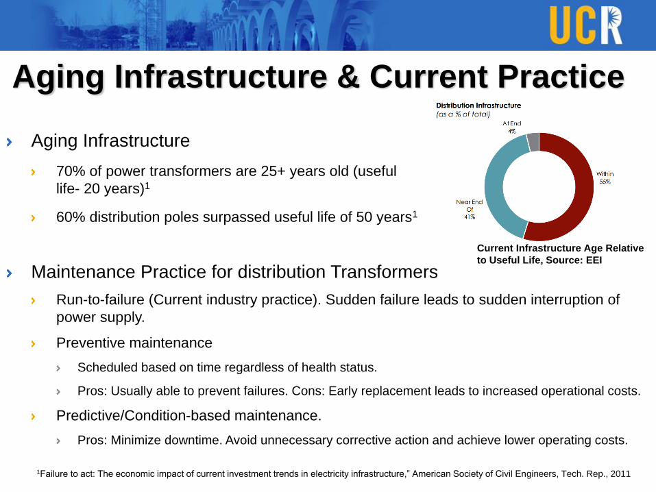
Aging Infrastructure & Current Practice
Aging Infrastructure
70% of power transformers are 25+ years old (useful
life- 20 years)1
60% distribution poles surpassed useful life of 50 years1
Current Infrastructure Age Relative
to Useful Life, Source: EEI
1Failure to act: The economic impact of current investment trends in electricity infrastructure,” American Society of Civil Engineers, Tech. Rep., 2011
Maintenance Practice for distribution Transformers
Run-to-failure (Current industry practice). Sudden failure leads to sudden interruption of
power supply.
Preventive maintenance
Scheduled based on time regardless of health status.
Pros: Usually able to prevent failures. Cons: Early replacement leads to increased operational costs.
Predictive/Condition-based maintenance.
Pros: Minimize downtime. Avoid unnecessary corrective action and achieve lower operating costs.
Challenge, Solution, and GoalChallenge
Predictive maintenance for large power transformers: a combination of dissolved gas
analysis (DGA) and data-driven machine learning techniques.
Requires semiconductor gas sensors for each transformer.
Suitable for transmission system. Not economically feasible for distribution system.
Solution: Use low cost and readily available data
Environmental condition, Transformer specification, Historical Failure
Transformer location information (GIS), Loading information (AMI)
Goal of the Study
Predict which transformers will fail in a given time horizon
Supervised binary classification task
Keep number of false positives low. Unexploited lifetime, increase in operating cost.
False negative has low cost
‘Match in top N’ (MITN) metric suitable
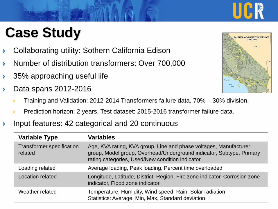
Case StudyCollaborating utility: Sothern California Edison
Number of distribution transformers: Over 700,000
35% approaching useful life
Data spans 2012-2016
Training and Validation: 2012-2014 Transformers failure data. 70% – 30% division.
Prediction horizon: 2 years. Test dataset: 2015-2016 transformer failure data.
Input features: 42 categorical and 20 continuous
Variable Type Variables
Transformer specification
related
Age, KVA rating, KVA group, Line and phase voltages, Manufacturer
group, Model group, Overhead/Underground indicator, Subtype, Primary
rating categories, Used/New condition indicator
Loading related Average loading, Peak loading, Percent time overloaded
Location related Longitude, Latitude, District, Region, Fire zone indicator, Corrosion zone
indicator, Flood zone indicator
Weather related Temperature, Humidity, Wind speed, Rain, Solar radiation
Statistics: Average, Min, Max, Standard deviation

MethodologyMissing Value Replacement
5% - 20% of weather, transformer location, loading, and specification data missing
MissForest method (non-parametric mixed-type imputation method)
Feature Selection
Wrapper Models: Forward/Backward search
Filter Models: Mutual information, Pearson correlation coefficient
Dealing with Imbalanced Dataset
RUSBoost integrates two algorithms
Random under-sampling of majority class
Boosting Tree
Ensemble of models
Assign higher weights to misclassified instances
AdaBoost M.2 algorithm
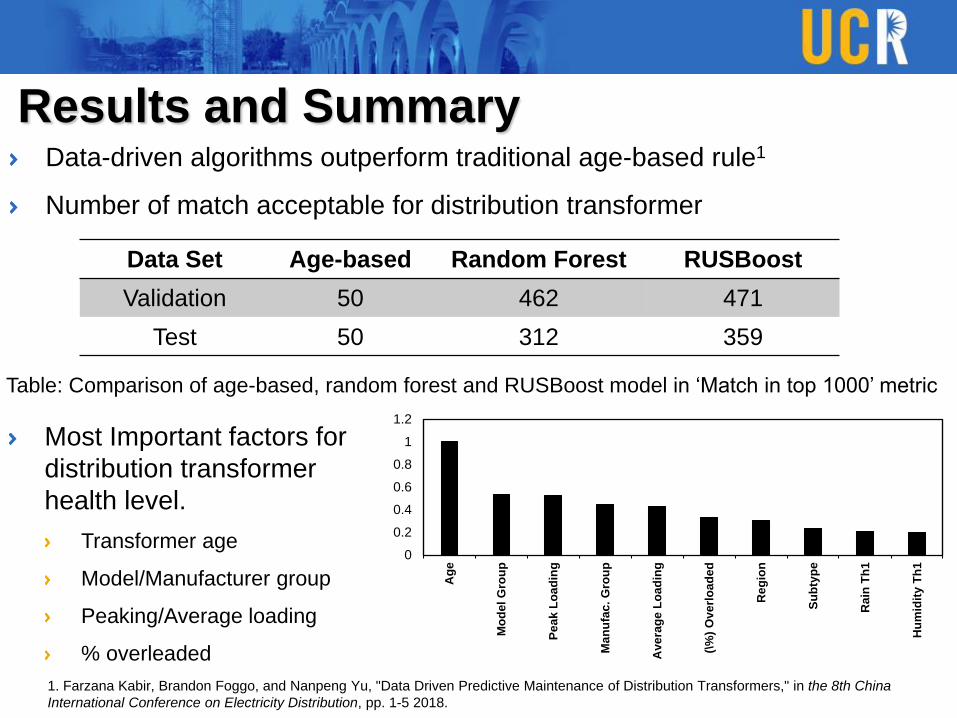
Results and SummaryData-driven algorithms outperform traditional age-based rule1
Number of match acceptable for distribution transformer
Data Set Age-based Random Forest RUSBoost
Validation 50 462 471
Test 50 312 359
Table: Comparison of age-based, random forest and RUSBoost model in ‘Match in top 1000’ metric
0
0.2
0.4
0.6
0.8
1
1.2
Ag
e
Mo
del G
rou
p
Pe
ak L
oa
din
g
Man
ufa
c. G
rou
p
Av
era
ge L
oad
ing
(\%
) O
verl
oad
ed
Reg
ion
Su
bty
pe
Rain
Th
1
Hu
mid
ity T
h1
Most Important factors for
distribution transformer
health level.
Transformer age
Model/Manufacturer group
Peaking/Average loading
% overleaded
1. Farzana Kabir, Brandon Foggo, and Nanpeng Yu, "Data Driven Predictive Maintenance of Distribution Transformers," in the 8th China
International Conference on Electricity Distribution, pp. 1-5 2018.

OutlineWhy do we focus on electric power distribution systems?
Big Data in Power Distribution Systems
Volume, Variety, Velocity, and Value
Applications of Machine Learning and Big Data Analytics in Power
Distribution Systems
Topology Identification – Phase Connectivity Identification
Anomaly Detection – Electricity Theft Detection
Reinforcement Learning based Control – Volt-VAR Control
Predictive Maintenance – Distribution Transformers
Estimation of Behind-the-meter Solar Generation

MotivationResidential solar PV adoptions are increasing rapidly around the world.
Most residential solar PV systems are deployed behind the smart meters
installed by the electric utilities.
Utilities often only collect the net load data.
Lack of visibility brings many operational and planning challenges.
An accurate estimation of solar PV generation is crucial to an array of
distribution system planning and operation activities.
Hosting capacity analysis
Feeder/substation net load forecasting
Volt-VAR control
Net Metering
𝑛𝑒𝑡 𝑙𝑜𝑎𝑑 = 𝑙𝑜𝑎𝑑 − 𝑠𝑜𝑙𝑎𝑟 𝑔𝑒𝑛𝑒𝑟𝑎𝑡𝑖𝑜𝑛
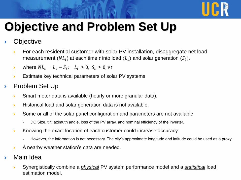
Objective and Problem Set UpObjective
For each residential customer with solar PV installation, disaggregate net load
measurement (𝑁𝐿𝑡) at each time 𝑡 into load (𝐿𝑡) and solar generation (𝑆𝑡).
where 𝑁𝐿𝑡 = 𝐿𝑡 − 𝑆𝑡; 𝐿𝑡 ≥ 0, 𝑆𝑡 ≥ 0, ∀𝑡
Estimate key technical parameters of solar PV systems
Problem Set Up
Smart meter data is available (hourly or more granular data).
Historical load and solar generation data is not available.
Some or all of the solar panel configuration and parameters are not available
DC Size, tilt, azimuth angle, loss of the PV array, and nominal efficiency of the inverter.
Knowing the exact location of each customer could increase accuracy.
However, the information is not necessary. The city’s approximate longitude and latitude could be used as a proxy.
A nearby weather station’s data are needed.
Main Idea
Synergistically combine a physical PV system performance model and a statistical load
estimation model.
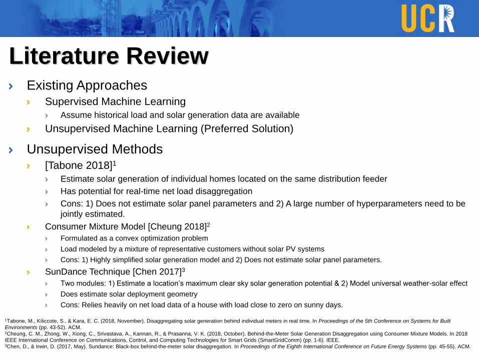
Literature ReviewExisting Approaches
Supervised Machine Learning
Assume historical load and solar generation data are available
Unsupervised Machine Learning (Preferred Solution)
Unsupervised Methods[Tabone 2018]1
Estimate solar generation of individual homes located on the same distribution feeder
Has potential for real-time net load disaggregation
Cons: 1) Does not estimate solar panel parameters and 2) A large number of hyperparameters need to be
jointly estimated.
Consumer Mixture Model [Cheung 2018]2
Formulated as a convex optimization problem
Load modeled by a mixture of representative customers without solar PV systems
Cons: 1) Highly simplified solar generation model and 2) Does not estimate solar panel parameters.
SunDance Technique [Chen 2017]3
Two modules: 1) Estimate a location’s maximum clear sky solar generation potential & 2) Model universal weather-solar effect
Does estimate solar deployment geometry
Cons: Relies heavily on net load data of a house with load close to zero on sunny days.
1Tabone, M., Kiliccote, S., & Kara, E. C. (2018, November). Disaggregating solar generation behind individual meters in real time. In Proceedings of the 5th Conference on Systems for Built
Environments (pp. 43-52). ACM.2Cheung, C. M., Zhong, W., Xiong, C., Srivastava, A., Kannan, R., & Prasanna, V. K. (2018, October). Behind-the-Meter Solar Generation Disaggregation using Consumer Mixture Models. In 2018
IEEE International Conference on Communications, Control, and Computing Technologies for Smart Grids (SmartGridComm) (pp. 1-6). IEEE.3Chen, D., & Irwin, D. (2017, May). Sundance: Black-box behind-the-meter solar disaggregation. In Proceedings of the Eighth International Conference on Future Energy Systems (pp. 45-55). ACM.

Overall Framework1
The net load includes two
components
The electric load and solar generation
Estimate one of the two components
at a time while fixing the other
component.
Solar generation is estimated by a
physical model with technical
parameters of solar PV systems.
The electric load is estimated based
on a statistical model.
Post-disaggregation adjustment
needed to ensure electric load minus
solar generation equals net load
measurement at all times.
Estimation of solar PV
parameters and solar generation
Load Estimation
Stopping
criteria
Post Disaggregation
adjustment
Disaggregation MethodNet load time series data
of a consumer
no
Disaggregated signals
Disaggregated signals
yes
Physical
model
Statistical
model
1Farzana Kabir, Nanpeng Yu, Weixin Yao, Rui Yang and Yingchen Zhang, “Estimation of Behind-the-Meter Solar Generation by Integrating Physical with
Statistical Models” to appear in IEEE SmartGridComm, pp. 1-5, Beijing, China, 2019.
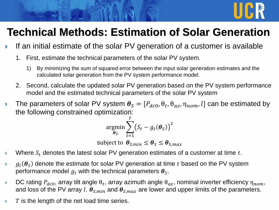
Technical Methods: Estimation of Solar Generation
If an initial estimate of the solar PV generation of a customer is available
1. First, estimate the technical parameters of the solar PV system.
1) By minimizing the sum of squared error between the input solar generation estimates and the
calculated solar generation from the PV system performance model.
2. Second, calculate the updated solar PV generation based on the PV system performance
model and the estimated technical parameters of the solar PV system
The parameters of solar PV system 𝜽𝑆 = [𝑃𝑑𝑐0, θ𝑡 , θ𝑎𝑧 , η𝑛𝑜𝑚, 𝑙] can be estimated by
the following constrained optimization:
argmin𝜽𝑆
𝑡=1
𝑇
𝑆𝑡 − 𝑔𝑡 𝜽𝑆2
subject to 𝜽𝑆,𝑚𝑖𝑛 ≤ 𝜽𝑆 ≤ 𝜽𝑆,𝑚𝑎𝑥
Where 𝑆𝑡 denotes the latest solar PV generation estimates of a customer at time 𝑡.
𝑔𝑡 𝜽𝑆 denote the estimate for solar PV generation at time 𝑡 based on the PV system
performance model 𝑔𝑡 with the technical parameters 𝜽𝑆.
DC rating 𝑃𝑑𝑐0, array tilt angle θ𝑡, array azimuth angle θ𝑎𝑧, nominal inverter efficiency η𝑛𝑜𝑚,
and loss of the PV array 𝑙. 𝜽𝑆,𝑚𝑖𝑛 and 𝜽𝑆,𝑚𝑎𝑥 are lower and upper limits of the parameters.
𝑇 is the length of the net load time series.
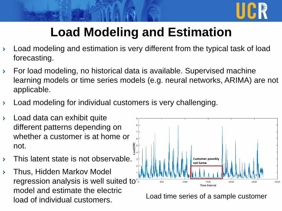
Load Modeling and Estimation
Load modeling and estimation is very different from the typical task of load
forecasting.
For load modeling, no historical data is available. Supervised machine
learning models or time series models (e.g. neural networks, ARIMA) are not
applicable.
Load modeling for individual customers is very challenging.
Load time series of a sample customer
Load data can exhibit quite
different patterns depending on
whether a customer is at home or
not.
This latent state is not observable.
Thus, Hidden Markov Model
regression analysis is well suited to
model and estimate the electric
load of individual customers.
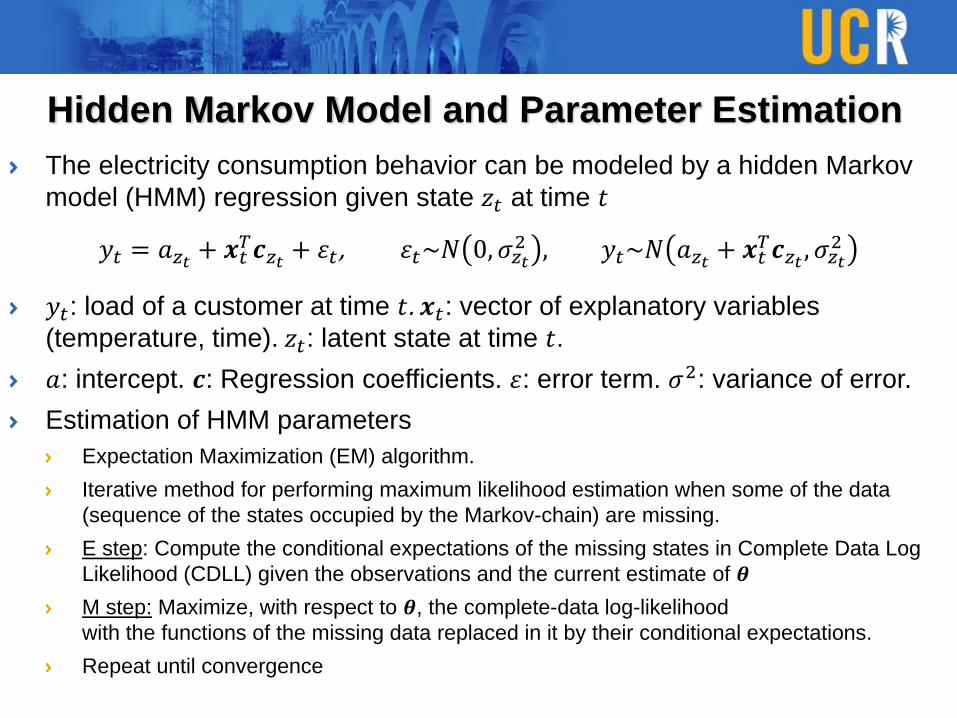
Hidden Markov Model and Parameter Estimation
The electricity consumption behavior can be modeled by a hidden Markov
model (HMM) regression given state 𝑧𝑡 at time 𝑡
𝑦𝑡 = 𝑎𝑧𝑡 + 𝒙𝑡𝑇𝒄𝑧𝑡 + 휀𝑡 , 휀𝑡~𝑁 0, 𝜎𝑧𝑡
2 , 𝑦𝑡~𝑁 𝑎𝑧𝑡 + 𝒙𝑡𝑇𝒄𝑧𝑡 , 𝜎𝑧𝑡
2
𝑦𝑡: load of a customer at time 𝑡. 𝒙𝑡: vector of explanatory variables
(temperature, time). 𝑧𝑡: latent state at time 𝑡.
𝑎: intercept. 𝒄: Regression coefficients. 휀: error term. 𝜎2: variance of error.
Estimation of HMM parameters
Expectation Maximization (EM) algorithm.
Iterative method for performing maximum likelihood estimation when some of the data
(sequence of the states occupied by the Markov-chain) are missing.
E step: Compute the conditional expectations of the missing states in Complete Data Log
Likelihood (CDLL) given the observations and the current estimate of 𝜽
M step: Maximize, with respect to 𝜽, the complete-data log-likelihood
with the functions of the missing data replaced in it by their conditional expectations.
Repeat until convergence

Post-Disaggregation Adjustment
To enforce that load minus generation is equal to net load at any time, we
do the following post-disaggregation adjustment
Calculate hyperparameters
Two variations
Known error variance: ground truth load and solar generation known for 10% of
consumers
Unknown error variance: Assume that ground truth load and solar generation
are the estimates from steps 4 and 7 of Algorithm 1
22
, 0
ˆˆarg min ' '
subject to 0, 0,
t t
T
t t t tL S t
t t t t t
L L S S
L S L S NL
1 1
' , 'Load PVVar Var

Numerical StudyData set
15-minute interval data from Pecan Street Dataset
Net load, load, and solar PV generation, DC size data
Location of customers: Austin Texas
Study period: Oct 3, 2015 – Oct 30, 2015 (28 days)
Number of customers with PV installations: 197
Solar irradiance and temperature data: National Solar Radiation Database
Feasible ranges of solar PV system parameters θ𝑆 specified
θ𝑇 ∈ [5°, 50°], θ𝐴𝑍 ∈ [0°, 360°], 𝑃𝑑𝑐0 ∈ [1𝐾𝑊, 15𝐾𝑊], η𝑛𝑜𝑚 ∈ [9%, 38%]
Initial values for solar PV system’s technical parameters
θ𝑇 , θ𝐴𝑍, η𝑛𝑜𝑚, 𝑙 set at their most common values
Gradually increase 𝑃𝑑𝑐0 from 1KW to 8 KW
Compared the estimation results with consumer mixture model and SunDance model
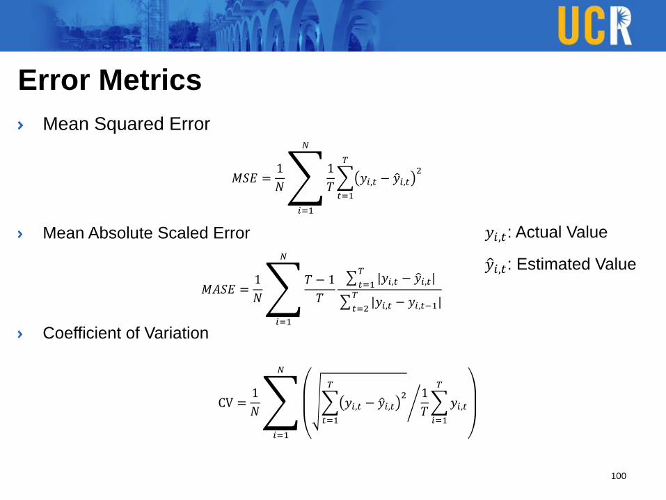
Error Metrics
Mean Squared Error
Mean Absolute Scaled Error
Coefficient of Variation
100
𝑀𝑆𝐸 =1
𝑁ා
𝑖=1
𝑁
1
𝑇
𝑡=1
𝑇
𝑦𝑖,𝑡 − ො𝑦𝑖,𝑡2
𝑀𝐴𝑆𝐸 =1
𝑁ා
𝑖=1
𝑁
𝑇 − 1
𝑇
𝑡=1
𝑇|𝑦𝑖,𝑡 − ො𝑦𝑖,𝑡|
𝑡=2
𝑇|𝑦𝑖,𝑡 − 𝑦𝑖,𝑡−1|
CV =1
𝑁ා
𝑖=1
𝑁
൙
𝑡=1
𝑇
𝑦𝑖,𝑡 − ො𝑦𝑖,𝑡2 1
𝑇
𝑖=1
𝑇
𝑦𝑖,𝑡
𝑦𝑖,𝑡: Actual Value
ො𝑦𝑖,𝑡: Estimated Value
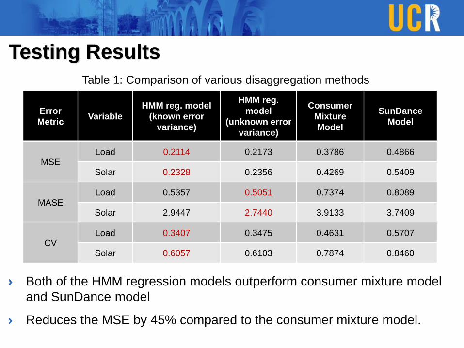
Testing Results
Both of the HMM regression models outperform consumer mixture model
and SunDance model
Reduces the MSE by 45% compared to the consumer mixture model.
Error
MetricVariable
HMM reg. model
(known error
variance)
HMM reg.
model
(unknown error
variance)
Consumer
Mixture
Model
SunDance
Model
MSELoad 0.2114 0.2173 0.3786 0.4866
Solar 0.2328 0.2356 0.4269 0.5409
MASELoad 0.5357 0.5051 0.7374 0.8089
Solar 2.9447 2.7440 3.9133 3.7409
CVLoad 0.3407 0.3475 0.4631 0.5707
Solar 0.6057 0.6103 0.7874 0.8460
Table 1: Comparison of various disaggregation methods

Testing Results
Reduction of MSE is 52% for these customers
HMM regression model is well suited to capture load behavior in different
regimes.
Performance Improvement is significant for customers who are absent from
home for an extended period
There are 25 such customers out of 197 customers with PV installation.
Comparison of disaggregated load and solar PV generation with actual values for a customer
from Oct 14 to Oct 19, 2015.
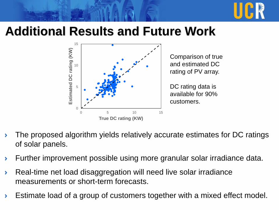
Additional Results and Future Work
The proposed algorithm yields relatively accurate estimates for DC ratings
of solar panels.
Further improvement possible using more granular solar irradiance data.
Real-time net load disaggregation will need live solar irradiance
measurements or short-term forecasts.
Estimate load of a group of customers together with a mixed effect model.
0
5
10
15
0 5 10 15
Esti
mate
d D
C r
ati
ng
(K
W)
True DC rating (KW)
Comparison of true
and estimated DC
rating of PV array.
DC rating data is
available for 90%
customers.

Thank You
Nanpeng Yu, Associate Professor
Department of Electrical and Computer Engineering
Department of Computer Science
Department of Statistics (cooperating faculty)
Website: https://intra.ece.ucr.edu/~nyu/
Email: [email protected]
Phone: 951.827.3688
Publications: Big Data Analytics & Machine Learning in Smart Grid1. N. Yu, S. Shah, R. Johnson, R. Sherick, Mingguo Hong and Kenneth Loparo, "Big Data Analytics in Power Distribution Systems", IEEE PES
Conference on Intelligent Smart Grid Technology, Washington DC, Feb. 2015.
2. Xiaoyang Zhou, Nanpeng Yu, Weixin Yao and Raymond Johnson, “Forecast load impact from demand response resources” Power and Energy
Society General Meeting, pp. 1-5, Boston, USA, 2016.
3. W. Wang, N. Yu, B. Foggo, and J. Davis, “Phase identification in electric power distribution systems by clustering of smart meter data” 15th IEEE
International Conference on Machine Learning and Applications (ICMLA), pp. 1-7, Anaheim, CA, 2016.
4. Jie Shi and Nanpeng Yu, “Spatio-temporal modeling of electric loads” in 49th North American Power Symposium, pp.1-6, Morgantown, WV, 2017.
5. W. Wang, N. Yu, and R. Johnson “A model for commercial adoption of photovoltaic systems in California” Journal of Renewable and Sustainable
Energy, Vol. 9, Issue, 2, pp.1-15, 2017.
6. Yuanqi Gao and Nanpeng Yu, “State estimation for unbalanced electric power distribution systems using AMI data” The Eighth Conference on
Innovative Smart Grid Technologies (ISGT 2017), pp. 1-5, Arlington, VA.
7. Wenyu. Wang and Nanpeng Yu, "AMI Data Driven Phase Identification in Smart Grid," the Second International Conference on Green
Communications, Computing and Technologies, pp. 1-8, Rome, Italy, Sep. 2017.
8. Jinhui Yang, Nanpeng Yu, Weixin Yao, Alec Wong, Larry Juang, and Raymond Johnson, “Evaluate the effectiveness of CVR with robust
regression” in Probabilistic Methods Applied to Power Systems, pp.1-6, 2018.
9. Brandon Foggo, Nanpeng Yu, “A comprehensive evaluation of supervised machine learning for the phase identification problem”, the 20th
International Conference on Machine Learning and Applications, pp.1-9, Copenhagen, Denmark, 2018.
10. Ke Wang, Haiwang Zhong, Nanpeng Yu, and Qing Xia, “Nonintrusive load monitoring based on sequence-to-sequence model with attention
mechanism”, Proceedings of the CSEE, 2018.
11. Farzana Kabir, Brandon Foggo, and Nanpeng Yu, "Data Driven Predictive Maintenance of Distribution Transformers," in the 8th China
International Conference on Electricity Distribution, pp. 1-5 2018.
12. Wei Wang and Nanpeng Yu, " A Machine Learning Framework for Algorithmic Trading with Virtual Bids in Electricity Markets," to appear in IEEE
Power and Energy Society General Meeting, 2019.
13. Yuanqi Gao, Brandon Foggo, and Nanpeng Yu, “A physically inspired data-driven model for electricity theft detection with smart meter data” to
appear in IEEE Transactions on Industrial Informatics, 2019.
14. Wang, Wenyu, and Nanpeng Yu. "Maximum Marginal Likelihood Estimation of Phase Connections in Power Distribution Systems." arXiv preprint
arXiv:1902.09686 (2019).
https://intra.ece.ucr.edu/~nyu/
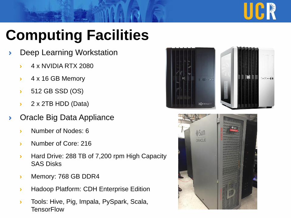
Computing FacilitiesDeep Learning Workstation
4 x NVIDIA RTX 2080
4 x 16 GB Memory
512 GB SSD (OS)
2 x 2TB HDD (Data)
Oracle Big Data Appliance
Number of Nodes: 6
Number of Core: 216
Hard Drive: 288 TB of 7,200 rpm High Capacity
SAS Disks
Memory: 768 GB DDR4
Hadoop Platform: CDH Enterprise Edition
Tools: Hive, Pig, Impala, PySpark, Scala,
TensorFlow