MAchine and Unite States Implementation

Copyright 2008 ISA. All rights reserved.

ISA–TR88.00.02

Machine and Unit States: An Implementation Example of

ISA-88

Approved 1 August 2008


ISA–TR88.00.02 Machine and Unit States: An Implementation Example of ISA-88 ISBN: 978-1-934394-81-6 Copyright © 2008 by ISA. All rights reserved. Not for resale. Printed in the United States of America. No part of this publication may be reproduced, stored in a retrieval system, or transmitted in any form or by any means (electronic, mechanical, photocopying, recording, or otherwise), without the prior written permission of the Publisher. ISA 67 Alexander Drive P. O. Box 12277 Research Triangle Park, NC 27709 USA

– 3 – ISA–TR88.00.02


Preface

This preface, as well as all footnotes and annexes, is included for information purposes and is not part of ISA-TR88.00.02. This document has been prepared as part of the service of ISA--The Instrumentation, Systems, and Automation Society--toward a goal of uniformity in the field of instrumentation. To be of real value, this document should not be static but should be subject to periodic review. Toward this end, the Society welcomes all comments and criticisms and asks that they be addressed to the Secretary, Standards and Practices Board; ISA; 67 Alexander Drive; P. O. Box 12277; Research Triangle Park, NC 27709; Telephone (919) 549-8411; Fax (919) 549-8288; Email: [email protected]. The ISA Standards and Practices Department is aware of the growing need for attention to the metric system of units in general, and the International System of Units (SI) in particular, in the preparation of instrumentation standards. The Department is further aware of the benefits to USA users of ISA standards of incorporating suitable references to the SI (and the metric system) in their business and professional dealings with other countries. Toward this end, this Department will endeavor to introduce SI-acceptable metric units in all new and revised standards, recommended practices, and technical reports to the greatest extent possible. Standard for Use of the International System of Units (SI): The Modern Metric System, published by the American Society for Testing & Materials as IEEE/ASTM SI 10-97, and future revisions, will be the reference guide for definitions, symbols, abbreviations, and conversion factors. It is the policy of ISA to encourage and welcome the participation of all concerned individuals and interests in the development of ISA standards, recommended practices, and technical reports. Participation in the ISA standards-making process by an individual in no way constitutes endorsement by the employer of that individual, of ISA, or of any of the standards, recommended practices, and technical reports that ISA develops. CAUTION — ISA adheres to the policy of the American National Standards Institute with regard to patents. If ISA is informed of an existing patent that is required for use of the standard, it will require the owner of the patent to either grant a royalty-free license for use of the patent by users complying with the document or a license on reasonable terms and conditions that are free from unfair discrimination. EVEN IF ISA IS UNAWARE OF ANY PATENT COVERING THIS DOCUMENT, THE USER IS CAUTIONED THAT IMPLEMENTATION OF THE DOCUMENT MAY REQUIRE USE OF TECHNIQUES, PROCESSES, OR MATERIALS COVERED BY PATENT RIGHTS. ISA TAKES NO POSITION ON THE EXISTENCE OR VALIDITY OF ANY PATENT RIGHTS THAT MAY BE INVOLVED IN IMPLEMENTING THE DOCUMENT. ISA IS NOT RESPONSIBLE FOR IDENTIFYING ALL PATENTS THAT MAY REQUIRE A LICENSE BEFORE IMPLEMENTATION OF THE DOCUMENT OR FOR INVESTIGATING THE VALIDITY OR SCOPE OF ANY PATENTS BROUGHT TO ITS ATTENTION. THE USER SHOULD CAREFULLY INVESTIGATE RELEVANT PATENTS BEFORE USING THE DOCUMENT FOR THE USER’S INTENDED APPLICATION. However, ISA asks that anyone reviewing this document who is aware of any patents that may impact implementation of the document notify the ISA Standards and Practices Department of the patent and its owner.

Additionally, the use of this document may involve hazardous materials, operations or equipment. The document cannot anticipate all possible applications or address all possible safety issues associated with use in hazardous conditions. The user of this document must exercise sound professional judgment concerning its use and applicability under the user’s particular circumstances. The user must also consider the applicability of any governmental regulatory limitations and established safety and health practices before implementing this document.

ISA–TR88.00.02 – 4 –


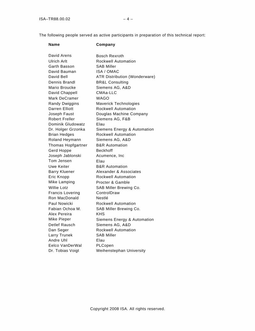
The following people served as active participants in preparation of this technical report:

Name Company David Arens Bosch Rexroth Ulrich Arlt Rockwell Automation Garth Basson SAB Miller David Bauman ISA / OMAC David Bell ATR Distribution (Wonderware) Dennis Brandl BR&L Consulting Mario Broucke Siemens AG, A&D David Chappell CMAa-LLC Mark DeCramer WAGO Randy Dwiggins Maverick Technologies Darren Elliott Rockwell Automation Joseph Faust Douglas Machine Company Robert Freller Siemens AG, F&B Dominik Gludowatz Elau Dr. Holger Grzonka Siemens Energy & Automation Brian Hedges Rockwell Automation Roland Heymann Siemens AG, A&D Thomas Hopfgartner B&R Automation Gerd Hoppe Beckhoff Joseph Jablonski Acumence, Inc Tom Jensen Elau Uwe Keiter B&R Automation Barry Kluener Alexander & Associates Eric Knopp Rockwell Automation Mike Lamping Procter & Gamble Willie Lotz SAB Miller Brewing Co. Francis Lovering ControlDraw Ron MacDonald Nestlé Paul Nowicki Rockwell Automation Fabian Ochoa M. SAB Miller Brewing Co. Alex Pereira KHS Mike Pieper Siemens Energy & Automation Detlef Rausch Siemens AG, A&D Dan Seger Rockwell Automation Larry Trunek SAB Miller Andre Uhl Elau Eelco VanDerWal PLCopen Dr. Tobias Voigt Weihenstephan University

– 5 – ISA–TR88.00.02


Contents

1 Scope ........................................................................................................................ 12 2 References ................................................................................................................ 12 3 Overview ................................................................................................................... 13

3.1 Introduction ....................................................................................................... 13 3.2 Personnel and Environmental Protection ............................................................ 14

4 Unit/Machine States ................................................................................................... 15 4.1 Definition .......................................................................................................... 15 4.2 Types of States ................................................................................................. 15 4.3 Defined States .................................................................................................. 15 4.4 State Transitions and State Commands .............................................................. 18

4.4.1 Definition ............................................................................................... 18 4.4.2 Types of State Commands...................................................................... 18 4.4.3 Examples of State Transitions ................................................................ 19

4.5 State Model....................................................................................................... 22 4.5.1 Base State Model................................................................................... 22

5 Modes ....................................................................................................................... 23 5.1 Unit/Machine Control Modes .............................................................................. 23 5.2 Unit / Machine Control Mode Management .......................................................... 25

6 Common Unit/Machine Mode Examples ....................................................................... 26 6.1 Producing Mode ................................................................................................ 26 6.2 Maintenance Mode ............................................................................................ 26 6.3 Manual Mode .................................................................................................... 28 6.4 User Mode ........................................................................................................ 30

7 Automated Machine Functional Tag Description ........................................................... 31 7.1 Introduction to PackTags ................................................................................... 31 7.2 Tag Types......................................................................................................... 31 7.3 PackTags Name Strings..................................................................................... 32 7.4 Data Types, Units, and Ranges .......................................................................... 32

7.4.1 Structured Data Types............................................................................ 32 7.5 Tag Details ....................................................................................................... 32

7.5.1 Command Tags...................................................................................... 39 7.5.1.1 Command.UnitMode................................................................. 39 7.5.1.2 Command.UnitModeChangeRequest ......................................... 39 7.5.1.3 Command.MachSpeed ............................................................. 41 7.5.1.4 Command.MaterialInterlocks..................................................... 41 7.5.1.5 Command.CntrlCmd ................................................................. 42 7.5.1.6 Command.CmdChangeRequest ................................................ 42 7.5.1.7 Command.RemoteInterface[#] .................................................. 42 7.5.1.8 Command.Parameter[#]............................................................ 44 7.5.1.9 Command.Product[#] ................................................................ 46

7.5.2 Status Tags ........................................................................................... 50 7.5.2.1 Status.UnitModeCurrent ........................................................... 50 7.5.2.2 Status.UnitModeRequested ...................................................... 50 7.5.2.3 Status.UnitModeChangeInProcess ............................................ 50

ISA–TR88.00.02 – 6 –


7.5.2.4 Status.StateCurrent.................................................................. 51 7.5.2.5 Status.StateRequested............................................................. 51 7.5.2.6 Status.StateChangeInProcess .................................................. 52 7.5.2.7 Status.MachSpeed ................................................................... 52 7.5.2.8 Status.CurMachSpeed.............................................................. 52 7.5.2.9 Status.MaterialInterlocks .......................................................... 53 7.5.2.10 Status.RemoteInterface[#] ........................................................ 53 7.5.2.11 Status.Parameter[#] ................................................................. 55 7.5.2.12 Status.Product[#] ..................................................................... 57

7.5.3 Administration Tags ............................................................................... 60 7.5.3.1 Admin.Parameter[#] ................................................................. 60 7.5.3.2 Admin.Alarm[#] ........................................................................ 61 7.5.3.3 Admin.AlarmExtent................................................................... 62 7.5.3.4 Admin.AlarmHistory[#] .............................................................. 62 7.5.3.5 Admin.AlarmHistoryExtent ........................................................ 64 7.5.3.6 Admin.ModeCurrentTime[#] ...................................................... 64 7.5.3.7 Admin.ModeCumulativeTime[#]................................................. 64 7.5.3.8 Admin.StateCurrentTime[#,#] .................................................... 64 7.5.3.9 Admin.StateCumulativeTime[#,#] .............................................. 65 7.5.3.10 Admin.ProdConsumedCount[#] ................................................. 65 7.5.3.11 Admin.ProdProcessedCount[#] ................................................. 66 7.5.3.12 Admin.ProdDefectiveCount[#] ................................................... 67 7.5.3.13 Admin.AccTimeSinceReset ....................................................... 68 7.5.3.14 Admin.MachDesignSpeed......................................................... 69 7.5.3.15 Admin.PACDateTime................................................................ 69

8 Software Implementation Examples............................................................................. 70 8.1 Example 1......................................................................................................... 70

8.1.1 Example Details ..................................................................................... 70 8.2 Example 2......................................................................................................... 73

8.2.1 Overview ............................................................................................... 73 8.2.2 What is the Machine Template? .............................................................. 73 8.2.3 Programming Example ........................................................................... 74 8.2.4 Vertical integration ................................................................................. 76

8.3 Example 3......................................................................................................... 77 8.3.1 Example Details ..................................................................................... 77

8.4 Example 4......................................................................................................... 80 8.4.1 Overview ............................................................................................... 80 8.4.2 Automation Templates............................................................................ 80 8.4.3 HMI Templates....................................................................................... 83

8.5 Example 5......................................................................................................... 84 8.5.1 Overview ............................................................................................... 84

8.6 Example 6......................................................................................................... 86 8.6.1 Example Details ..................................................................................... 86 8.6.2 Graphic Example.................................................................................... 87

9 OEE Implementation Examples ................................................................................... 90 9.1 OEE Definition .................................................................................................. 90

9.1.1 Availability Definition .............................................................................. 91 9.1.2 Performance Definition ........................................................................... 91

– 7 – ISA–TR88.00.02


9.1.3 Quality Definition ................................................................................... 92 9.2 Calculating a Real-Time OEE in a Machine Controller or HMI .............................. 92

9.2.1 Availability ............................................................................................. 92 9.2.2 Performance .......................................................................................... 93 9.2.3 Quality................................................................................................... 93 9.2.4 Overall Real-Time OEE Calculation......................................................... 93 9.2.5 Limitations of Real-Time OEE Equation ................................................... 93

9.3 Calculating a Complex Historical OEE Using a Historical Database Based System ............................................................................................................. 93 9.3.1 Further Analysis of Performance ............................................................. 95

9.3.1.1 Low Speed Losses ................................................................... 95 9.3.1.2 Small Stop Losses ................................................................... 95 9.3.1.3 Mode or State Transition .......................................................... 95 9.3.1.4 Loop through the Active Alarm File ........................................... 96

9.3.2 Limitations of a Historical OEE Calculation .............................................. 96 9.4 DIN 8782 OEE Harmonization Example .............................................................. 97

9.4.1 Definitions ............................................................................................. 97 9.4.2 General Operational Efficiency Examples ................................................ 99

A.1 Alarm Codes ................................................................................................... 100 A.2 Weihenstephan Harmonization ......................................................................... 103

ISA–TR88.00.02 – 8 –


LIST OF FIGURES AND TABLES

Figure 1: Automated Machines applied to ISA88.00.01 Physical Model ............................... 13 Figure 2: Example States for Automated Machines............................................................. 16 Table 1 : Complete List of Machine States ......................................................................... 16 Table 2 : Example Transition Matrix of Local or Remote State Commands........................... 20 Table 3: Example Matrix of Machine Conditions Initiating a State Command........................ 21 Figure 3: Base State Model Visualization ........................................................................... 22 Figure 4: Unit/Machine Control Modes ............................................................................... 23 Figure 5: Multi-Mode Example Diagram (Producing Mode States) ....................................... 25 Figure 6: Maintenance Mode State Model ......................................................................... 26 Figure 7: Maintenance Mode Execution Model .................................................................. 27 Figure 8: Manual Mode State Model .................................................................................. 28 Figure 9: Manual Mode Execution Model .......................................................................... 29 Figure 10: Automatic Weihenstephan State Model.............................................................. 30 Figure 11: Tag Information Flow........................................................................................ 31 Table 4: Command Tags................................................................................................... 33 Table 5 : Status Tags ....................................................................................................... 35 Table 6 : Administration Tags............................................................................................ 37 Figure 12: Unit Mode Change Example Sequence.............................................................. 40 Figure 7: Unit Mode Change Example Sequence................................................................ 51 Figure 8: State Change Example Sequence ....................................................................... 52 Figure 9: Example 8.1 CPU Software Tree......................................................................... 70 Figure 10: Example 8.1 Initialization in Structured Text ...................................................... 71 Figure 11: Example 8.1 Visualization Sample of Operator Interface..................................... 72 Figure 12: Example 8.2 Visualization Sample of Production Mode....................................... 74 Figure 13: Example 8.2 Programming Sample of Mode Manager......................................... 74 Figure 14: Example 8.2 Sample Tag Structure ................................................................... 75 Figure 15: Example 8.2 Visualization Sample for Implementation Support ........................... 76 Figure 16: Example 8.3 Explorer View of Software ............................................................. 77 Figure 17: Example 8.3 State Routine Layout .................................................................... 78 Figure 18: Example 8.3 Partial Sequential Function Chart of State Engine .......................... 78 Figure 19: Example 8.3 PackTags User Defined Tags ........................................................ 79 Figure 20: Example 8.4 State Routine Template................................................................. 81 Figure 21: Example 8.4 Mode Manager Interface with Production Mode .............................. 82 Figure 22: Example 8.4 Status Tags Template Layout ........................................................ 83 Figure 23: Example 8.4 Operator Visualization for Base State Model .................................. 83 Figure 24: Example 8.5 PackML Template Block ................................................................ 84 Figure 25: Example 8.5 Structure Flow Chart for Base State Model..................................... 85 Figure 26: Example 8.6 Template Toolbox ......................................................................... 86 Figure 27: Example 8.6 Sequencer Program for Automatic Mode State Model ..................... 87 Figure 28: Example 8.6 Graphic Example of User Interface ................................................ 88

– 9 – ISA–TR88.00.02


Figure 29: Example 8.6 Unit Control .................................................................................. 88 Figure 30: Example 8.6 Parameter Array Structure............................................................. 89 Figure 31: Example 8.6 Product Array Structure................................................................. 89 Figure 39: OEE Waterfall Diagram..................................................................................... 90 Figure 40: DIN 8782 OEE Diagram.................................................................................... 97

ISA–TR88.00.02 – 10 –


Foreword

The ISA88 committee has defined a batch standard series that provides terminology and a consistent set of concepts and models for batch manufacturing plants and batch control. These standards, however, were not defined in the context of Packaging machines, or machines that perform discrete operations. As the ISA-88 batch standards continue to evolve, the context of the standard models may be extended to include the entire plant, integrating the software definitions of batch, packaging, converting and warehousing. Currently, as noted in this report there is a need to begin consideration of the ISA-88 standards in the context of differing automated machinery. This is an informative document. This document contains definitive implementation examples of definitions and models in order to establish a common presentation and high level software architecture or layout. The terms and definitions used in this document are harmonized, as much as possible, with ISA-88; the document is not definitive in this respect. The models used, and applied, in this document are an extension of the models presented in ISA-88 and are shown how they are applied to differing machine functionality. Discrete machine functionality is expressed graphically in several situations and described. The intent of this document is to propose specific implementation options and indicate a preference for a specific set of machine types.

Abstract

The “standard” method of programming discrete machines is generally considered to be solely dependent on the machine and the software engineer, or control systems programmer. This constant change offers little additional value and generally increases the total costs, from the designing and building of the process to operating and maintaining the system by the end user. This Technical Report on the implementation of ISA-88 in discrete machines breaks this paradigm and demonstrates how to apply the ISA-88 standard to discrete machine states and modes. The implementation of the standard will create a standard programming methodology as well as consistent method to install, communicate, operate, and maintain a piece of unit/machine. This Technical Report gives examples of general and specific machine state models and procedural methods. The report cites real control examples as implementations, and provides specific tag naming conventions; it also cites a number of common terms that are consistent with batch processing and ISA-88.

Key Words State machine, state model, mode manager, machine state, unit control mode, PackML, state commands, command tags, status tags, administration tags, base state model, state engine, functional programming, modular programming, machine control software, discrete machine software, PackTags, Weihenstephan, Production Data Acquisition, PDA, ISA88, and TR88.

– 11 – ISA–TR88.00.02


Introduction

When the ISA-88 standard is applied to applications across a plant, there is a need to align the terminologies, models, and key definitions between different process types; continuous, batch, and discrete processes. Discrete processes involve machines found in the packaging, converting, and material handling applications. The operation of these machines is typically defined by the OEM, system integrator, end user, or is industry specific. A task group with members from technology providers, OEMs, system integrators, and end users was chartered by the OMAC (Open Modular Architecture Control)/ISA Packaging Workgroup. The task group generated the PackML guidelines as a method to show how the ISA-88 concepts could be extended into packaging machinery. This technical report is intended to build upon and formalize the concepts of the PackML guidelines and to show application examples. The purpose of the technical report is to

a) Explain functional state programming for automated machines;

b) Identify definitions for common terminology;

c) Explain to practitioners how to use state programming for automated machines;

d) Provide actual implementation examples and templates from automation control vendors;

e) Identify a common tag structure for automated machines in order to:

1) Provide for Connect & Pack functionality;

2) Provide functional interoperability and a consistent look and feel across the plant floor;

3) Provide consistent tag structure for connection to plant MES and enterprise systems.

ISA–TR88.00.02 – 12 –


Machine and Unit States: An Implementation Example of ISA-88

1 Scope

Since its inception, the OMAC Packaging Machine Language (PackML) group has been using a variety of information sources and technical documents to define a common approach, or machine language, for automated machines. The primary goals are to encourage a common “look and feel” across a plant floor, and to enable and encourage industry innovation. The PackML group is recognized globally and consists of control vendors, OEM’s, system integrators, universities, and end users, which collaborate on definitions that endeavour to be consistent with the ISA88 standards and consistent with the technology and the changing needs of a majority of automated machinery. The term “machine” used in this report is equivalent to an ISA88 “Unit”. This has led to the following:

1. A definition of machine/unit state types. 2. A definition of machine/unit control modes. 3. A definition of unit control mode management. 4. State models, State descriptions, and transitions.

2 References

The following documents contain provisions that are referenced in this text. At the time of publication the editions indicated were valid. All documents are subject to revision, and parties to agreements based on this technical report are encouraged to investigate the possibility of applying the most recent editions of the reference documents indicated below. ⎯ ISA-88.00.01-1995,.Batch Control Part 1: Models and Terminologies

⎯ ANSI/ISA-88.00.02-2001 Batch Control Part 2: Data Structures and Guidelines for Languages

⎯ ANSI/ISA-88.00.03-2003 Batch Control Part 3: General and Site Recipe Models and Representation

⎯ ANSI/ISA-88.00.04-2006 Batch Control Part 4: Batch Production Records

⎯ ISA Draft 88.00.05 Batch Control - Part 5: Implementation Models & Terminology for Modular Equipment Control

⎯ IEC 61131-1 Standard for programmable logic controllers (PLCs), General Information

⎯ IEC 61131-3 Standard for programmable logic controllers (PLCs), Programming Languages

⎯ IEC 61131-4 Standard for programmable logic controllers (PLCs), User Guidelines

⎯ PLCopen TC5 Safety Certification

⎯ Weihenstephan Standard – Part 2 Version 2005 http://www.wzw.tum.de/lvt/englisch/Weihenstephaner_Standards_GB.html

⎯ ANSI/ISA-95.00.01-2000 Enterprise–Control System Integration Part 1: Models and Terminologies

⎯ ANSI/ISA-95.00.02-2001 Enterprise–Control System Integration Part 2: Object Model Attributes

⎯ ANSI/ISA-95.00.05, Enterprise-Control System Integration Part 5: Business-to- Manufacturing Transactions

⎯ DIN 8782, Beverage Packaging Technology: Terminology Associated with Filling Plants and their Constituent Machines

– 13 – ISA–TR88.00.02


3 Overview

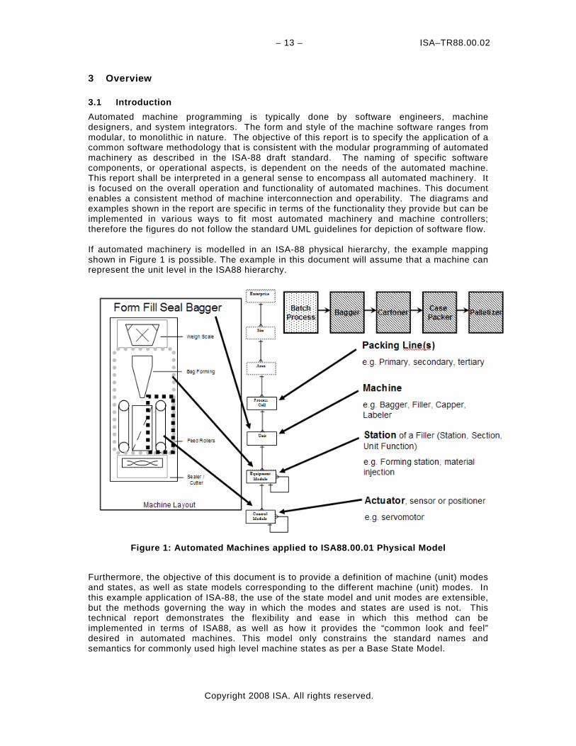
3.1 Introduction Automated machine programming is typically done by software engineers, machine designers, and system integrators. The form and style of the machine software ranges from modular, to monolithic in nature. The objective of this report is to specify the application of a common software methodology that is consistent with the modular programming of automated machinery as described in the ISA-88 draft standard. The naming of specific software components, or operational aspects, is dependent on the needs of the automated machine. This report shall be interpreted in a general sense to encompass all automated machinery. It is focused on the overall operation and functionality of automated machines. This document enables a consistent method of machine interconnection and operability. The diagrams and examples shown in the report are specific in terms of the functionality they provide but can be implemented in various ways to fit most automated machinery and machine controllers; therefore the figures do not follow the standard UML guidelines for depiction of software flow. If automated machinery is modelled in an ISA-88 physical hierarchy, the example mapping shown in Figure 1 is possible. The example in this document will assume that a machine can represent the unit level in the ISA88 hierarchy.

Figure 1: Automated Machines applied to ISA88.00.01 Physical Model

Furthermore, the objective of this document is to provide a definition of machine (unit) modes and states, as well as state models corresponding to the different machine (unit) modes. In this example application of ISA-88, the use of the state model and unit modes are extensible, but the methods governing the way in which the modes and states are used is not. This technical report demonstrates the flexibility and ease in which this method can be implemented in terms of ISA88, as well as how it provides the “common look and feel” desired in automated machines. This model only constrains the standard names and semantics for commonly used high level machine states as per a Base State Model.

ISA–TR88.00.02 – 14 –


The ISA-88 standard describes example modes and states as applied to equipment entities and procedural elements. This report identifies unit/machine modes and states which should be considered an extension of the examples in the ISA-88 standard in order to meet the needs of automated machine processing. 3.2 Personnel and Environmental Protection The Personnel and Environmental Protection control activity provides safety for people and the environment. No control activity should intervene between Personnel and Environmental Protection and the field hardware it is designed to operate with. Personnel and Environmental Protection is, by definition, separate from the higher level control activities in this document. It may map to more than one software level of the equipment as desired. A complete discussion of personnel and environmental protection, the classification of these types of systems, and the segregation of levels of interlocks within these systems is a topic of its own and beyond the scope of this document.

– 15 – ISA–TR88.00.02


4 Unit/Machine States

4.1 Definition A Unit/Machine state completely defines the current condition of a machine. A Machine state is expressed as an ordered procedure, or programming routine, that can consist of one or more commands to other Procedural Elements1 or equipment entities, or consist of the status of a Procedural Element1 or equipment entity, or both. In performing the function specified by the state the Machine state will issue a set of commands to the machine Procedural Elements1 or equipment entities which in turn can report status. The Machine state will perform conditional logic which will either lead to further execution within the current machine state or cause a transition to another state. The Machine state is the result of previous activities that had taken place in the machine to change the previous state. Only one major processing activity may be active in one machine at any time2. The linear sequence of major activities will drive a strictly sequentially ordered flow of control from one state to the next state – no parallel states operating on the same equipment entity are allowed to be active in one machine at the same time. Note: At a lower level, the minor sub-activities (or control procedures) that are combined to form a major activity at the machine operation level, may indeed be taking place in parallel as well as in sequence as defined in ISA- 88 for equipment phases.

4.2 Types of States For the purposes of understanding three machine state types are defined: • Acting State: A state which represents some processing activity. It implies the single or

repeated execution of processing steps in a logical order, for a finite time or until a specific condition has been reached. In ISA-88 these are referred to Transient states, those states ending in “-ing”.

• Wait State: A state used to identify that a machine has achieved a defined set of conditions. In such a state, the machine is maintaining a status until transitioning to an Acting state or the Dual state. In ISA-88 this was referred to as a Final or Quiescent state.

• Dual State: A Wait state that is causing the machine to behave as in an Acting state. The Dual state is representative of a Machine state that can be continuously transitioning between Acting and Waiting, and Looping, as defined by the logical sequence required. As noted in ISA-88, the Execute, or Running state, is a Transient state. This Machine state has been re-characterized to also include the diversity of operation found in packaging and discrete machines.

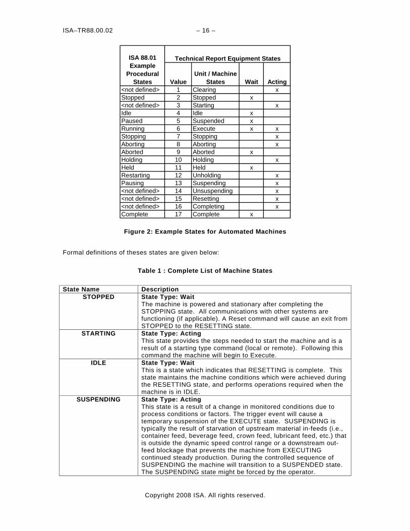
4.3 Defined States

There are a fixed number of states defined in the Base State Model. This report establishes an example enumerated set of possible Unit/Machine states illustrated in the figure below, Figure 2. As shown this set of states has similarity to the ISA-88 example states, but has additional states defined for machine processing.

————————— 1 Term Procedural Element defined (ISA-88)

2 A “major processing activity,” corresponds to the term Equipment Operation as defined in ISA-88.

ISA–TR88.00.02 – 16 –


ValueUnit / Machine

States Wait Acting<not defined> 1 Clearing xStopped 2 Stopped x<not defined> 3 Starting xIdle 4 Idle xPaused 5 Suspended xRunning 6 Execute x xStopping 7 Stopping xAborting 8 Aborting xAborted 9 Aborted xHolding 10 Holding xHeld 11 Held xRestarting 12 Unholding xPausing 13 Suspending x<not defined> 14 Unsuspending x<not defined> 15 Resetting x<not defined> 16 Completing xComplete 17 Complete x

ISA 88.01 Example

Procedural States

Technical Report Equipment States

Figure 2: Example States for Automated Machines

Formal definitions of theses states are given below:

Table 1 : Complete List of Machine States

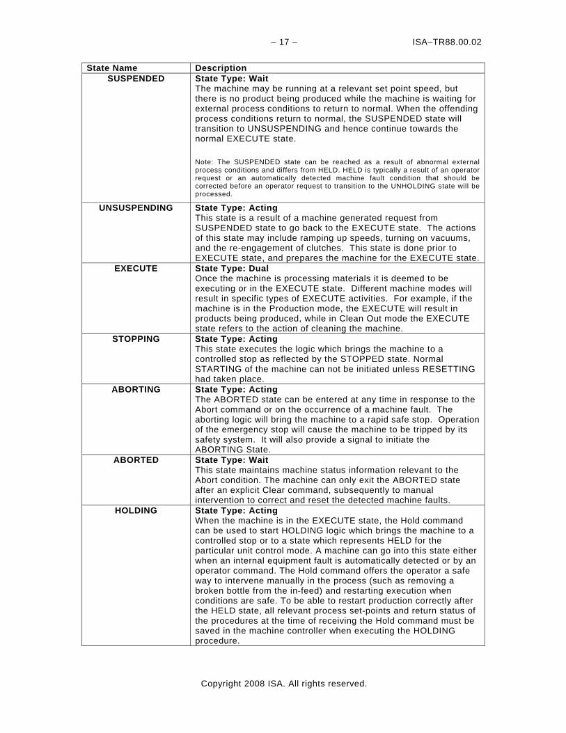
State Name Description

STOPPED State Type: Wait The machine is powered and stationary after completing the STOPPING state. All communications with other systems are functioning (if applicable). A Reset command will cause an exit from STOPPED to the RESETTING state.

STARTING State Type: Acting This state provides the steps needed to start the machine and is a result of a starting type command (local or remote). Following this command the machine will begin to Execute.

IDLE

State Type: Wait This is a state which indicates that RESETTING is complete. This state maintains the machine conditions which were achieved during the RESETTING state, and performs operations required when the machine is in IDLE.

SUSPENDING State Type: Acting This state is a result of a change in monitored conditions due to process conditions or factors. The trigger event will cause a temporary suspension of the EXECUTE state. SUSPENDING is typically the result of starvation of upstream material in-feeds (i.e., container feed, beverage feed, crown feed, lubricant feed, etc.) that is outside the dynamic speed control range or a downstream out-feed blockage that prevents the machine from EXECUTING continued steady production. During the controlled sequence of SUSPENDING the machine will transition to a SUSPENDED state. The SUSPENDING state might be forced by the operator.

– 17 – ISA–TR88.00.02


State Name Description SUSPENDED State Type: Wait

The machine may be running at a relevant set point speed, but there is no product being produced while the machine is waiting for external process conditions to return to normal. When the offending process conditions return to normal, the SUSPENDED state will transition to UNSUSPENDING and hence continue towards the normal EXECUTE state. Note: The SUSPENDED state can be reached as a result of abnormal external process conditions and differs from HELD. HELD is typically a result of an operator request or an automatically detected machine fault condition that should be corrected before an operator request to transition to the UNHOLDING state will be processed.

UNSUSPENDING State Type: Acting This state is a result of a machine generated request from SUSPENDED state to go back to the EXECUTE state. The actions of this state may include ramping up speeds, turning on vacuums, and the re-engagement of clutches. This state is done prior to EXECUTE state, and prepares the machine for the EXECUTE state.

EXECUTE State Type: Dual Once the machine is processing materials it is deemed to be executing or in the EXECUTE state. Different machine modes will result in specific types of EXECUTE activities. For example, if the machine is in the Production mode, the EXECUTE will result in products being produced, while in Clean Out mode the EXECUTE state refers to the action of cleaning the machine.

STOPPING State Type: Acting This state executes the logic which brings the machine to a controlled stop as reflected by the STOPPED state. Normal STARTING of the machine can not be initiated unless RESETTING had taken place.

ABORTING State Type: Acting The ABORTED state can be entered at any time in response to the Abort command or on the occurrence of a machine fault. The aborting logic will bring the machine to a rapid safe stop. Operation of the emergency stop will cause the machine to be tripped by its safety system. It will also provide a signal to initiate the ABORTING State.

ABORTED State Type: Wait This state maintains machine status information relevant to the Abort condition. The machine can only exit the ABORTED state after an explicit Clear command, subsequently to manual intervention to correct and reset the detected machine faults.

HOLDING State Type: Acting When the machine is in the EXECUTE state, the Hold command can be used to start HOLDING logic which brings the machine to a controlled stop or to a state which represents HELD for the particular unit control mode. A machine can go into this state either when an internal equipment fault is automatically detected or by an operator command. The Hold command offers the operator a safe way to intervene manually in the process (such as removing a broken bottle from the in-feed) and restarting execution when conditions are safe. To be able to restart production correctly after the HELD state, all relevant process set-points and return status of the procedures at the time of receiving the Hold command must be saved in the machine controller when executing the HOLDING procedure.

ISA–TR88.00.02 – 18 –


State Name Description HELD State Type: Wait

The HELD state holds the machine's operation while material blockages are cleared, or to stop throughput while a downstream problem is resolved, or enable the safe correction of an equipment fault before the production may be resumed.

UNHOLDING State Type: Acting The UNHOLDING state is a response to an Operator command to resume the EXECUTE state. Issuing the Unhold command will retrieve the saved set-points and return the status conditions to prepare the machine to re-enter the normal EXECUTE state. Note: An operator Unhold command is always required and UNHOLDING can never be initiated automatically.

COMPLETING State Type: Acting This state is an automatic response from the EXECUTE state. Normal operation has run to completion (i.e., processing of material at the infeed will stop).

COMPLETE State Type: Wait The machine has finished the COMPLETING state and is now waiting for a Reset command before transitioning to the RESETTING state.

RESETTING State Type: Acting This state is the result of a RESET command from the STOPPED or complete state. RESETTING will typically cause a machine to sound a horn and place the machine in a state where components are energized awaiting a START command.

CLEARING State Type: Acting Initiated by a state command to clear faults that may have occurred when ABORTING, and are present in the ABORTED state before proceeding to a STOPPED state.

4.4 State Transitions and State Commands

4.4.1 Definition

A State transition is defined as a passage from one state to another. Transitions between states will occur as a result of a local, remote, or procedural State command. State commands are procedural elements that in effect cause a state transition to occur.

4.4.2 Types of State Commands State commands are comprised of one or a combination of the following types:

• Operator intervention • Response to the status of one or more procedural elements • Response to machine conditions • The completion of an Acting state procedure • Supervisory or remote system intervention

– 19 – ISA–TR88.00.02


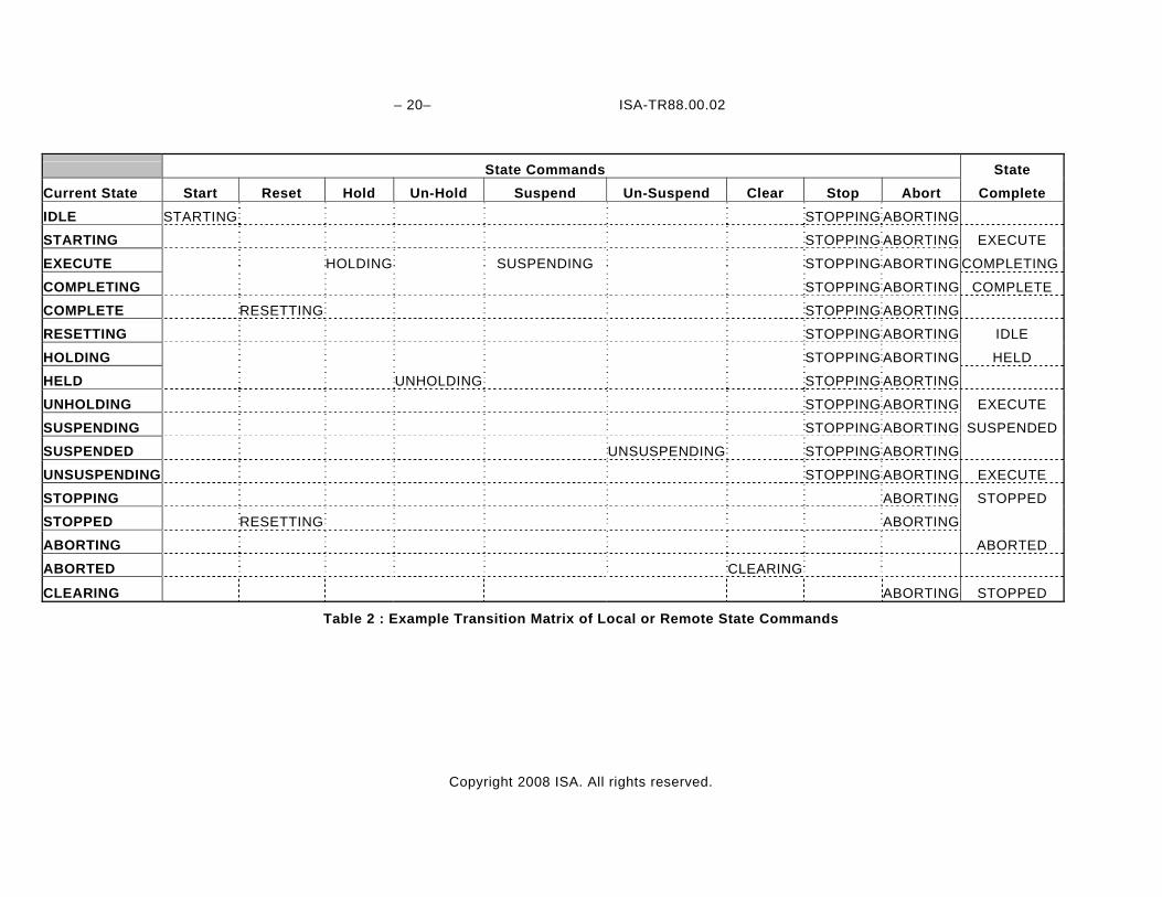
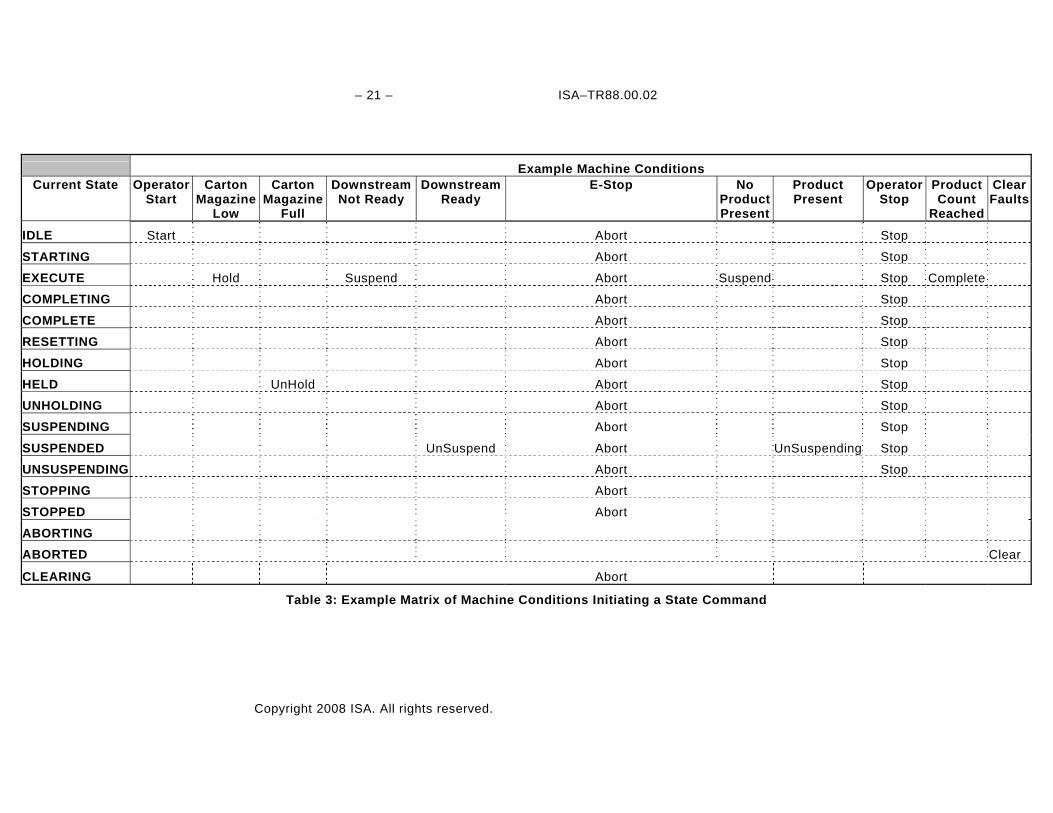
4.4.3 Examples of State Transitions An Example Transition Matrix for local or remote State commands generated by an operator is shown in Table 2. After every Acting state, as can be seen in Table 2, a procedural element is required that will indicate the Acting state is complete, or a command is required to stop or abort the Acting state. The State Complete indication within the Acting state procedure will cause a state transition to occur. Similarly, an Example State Command Matrix of machine conditions activating a State command is shown in Table 3. The objective of this table is to depict the machine conditions that will cause a state transition using the commands defined in Table 2.

– 20– ISA-TR88.00.02


State Commands State Current State Start Reset Hold Un-Hold Suspend Un-Suspend Clear Stop Abort Complete IDLE STARTING STOPPING ABORTING

STARTING STOPPING ABORTING EXECUTE

EXECUTE HOLDING SUSPENDING STOPPING ABORTING COMPLETING

COMPLETING STOPPING ABORTING COMPLETE

COMPLETE RESETTING STOPPING ABORTING

RESETTING STOPPING ABORTING IDLE

HOLDING STOPPING ABORTING HELD

HELD UNHOLDING STOPPING ABORTING

UNHOLDING STOPPING ABORTING EXECUTE

SUSPENDING STOPPING ABORTING SUSPENDED

SUSPENDED UNSUSPENDING STOPPING ABORTING

UNSUSPENDING STOPPING ABORTING EXECUTE

STOPPING ABORTING STOPPED

STOPPED RESETTING ABORTING

ABORTING ABORTED

ABORTED CLEARING

CLEARING ABORTING STOPPED

Table 2 : Example Transition Matrix of Local or Remote State Commands

– 21 – ISA–TR88.00.02


Example Machine Conditions Current State Operator

Start Carton

Magazine Low

Carton Magazine

Full

Downstream Not Ready

Downstream Ready

E-Stop No Product Present

Product Present

Operator Stop

Product Count

Reached

Clear Faults

IDLE Start Abort Stop

STARTING Abort Stop

EXECUTE Hold Suspend Abort Suspend Stop Complete

COMPLETING Abort Stop

COMPLETE Abort Stop

RESETTING Abort Stop

HOLDING Abort Stop

HELD UnHold Abort Stop

UNHOLDING Abort Stop

SUSPENDING Abort Stop

SUSPENDED UnSuspend Abort UnSuspending Stop

UNSUSPENDING Abort Stop

STOPPING Abort

STOPPED Abort

ABORTING

ABORTED Clear

CLEARING Abort

Table 3: Example Matrix of Machine Conditions Initiating a State Command

– 22– ISA-TR88.00.02


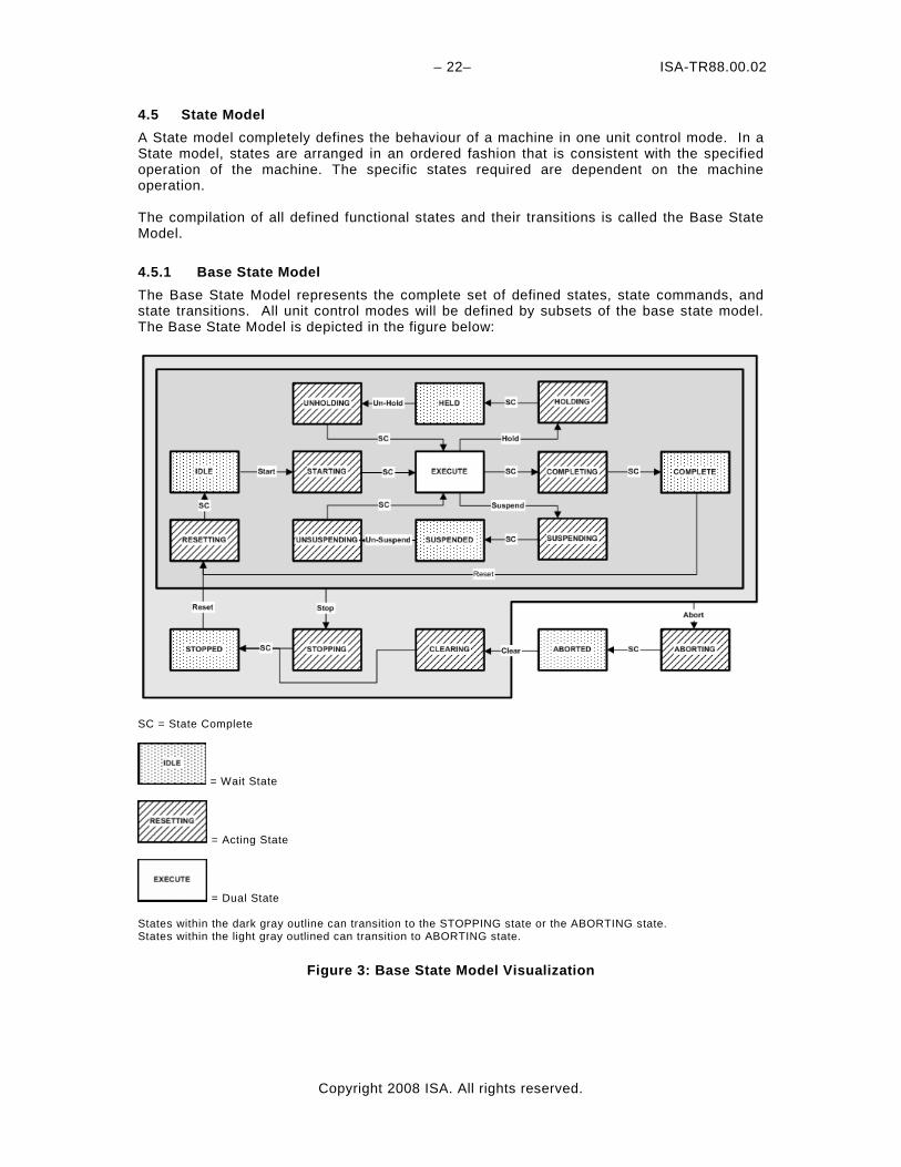
4.5 State Model A State model completely defines the behaviour of a machine in one unit control mode. In a State model, states are arranged in an ordered fashion that is consistent with the specified operation of the machine. The specific states required are dependent on the machine operation. The compilation of all defined functional states and their transitions is called the Base State Model. 4.5.1 Base State Model The Base State Model represents the complete set of defined states, state commands, and state transitions. All unit control modes will be defined by subsets of the base state model. The Base State Model is depicted in the figure below:

SC = State Complete

= Wait State

= Acting State

= Dual State States within the dark gray outline can transition to the STOPPING state or the ABORTING state. States within the light gray outlined can transition to ABORTING state.

Figure 3: Base State Model Visualization

– 23 – ISA–TR88.00.02


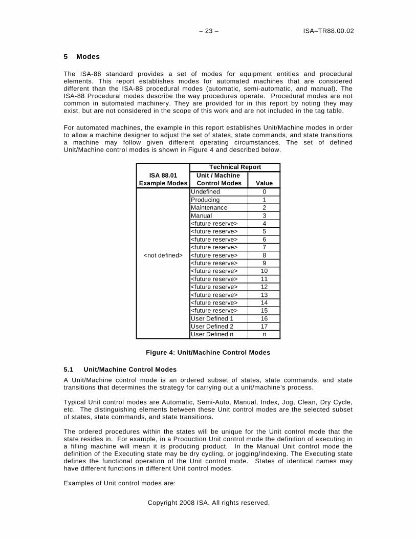
5 Modes

The ISA-88 standard provides a set of modes for equipment entities and procedural elements. This report establishes modes for automated machines that are considered different than the ISA-88 procedural modes (automatic, semi-automatic, and manual). The ISA-88 Procedural modes describe the way procedures operate. Procedural modes are not common in automated machinery. They are provided for in this report by noting they may exist, but are not considered in the scope of this work and are not included in the tag table.

For automated machines, the example in this report establishes Unit/Machine modes in order to allow a machine designer to adjust the set of states, state commands, and state transitions a machine may follow given different operating circumstances. The set of defined Unit/Machine control modes is shown in Figure 4 and described below.

ISA 88.01 Unit / Machine Example Modes Control Modes Value

Undefined 0Producing 1Maintenance 2Manual 3<future reserve> 4<future reserve> 5<future reserve> 6<future reserve> 7

<not defined> <future reserve> 8<future reserve> 9<future reserve> 10<future reserve> 11<future reserve> 12<future reserve> 13<future reserve> 14<future reserve> 15User Defined 1 16User Defined 2 17User Defined n n

Technical Report

Figure 4: Unit/Machine Control Modes

5.1 Unit/Machine Control Modes A Unit/Machine control mode is an ordered subset of states, state commands, and state transitions that determines the strategy for carrying out a unit/machine’s process. Typical Unit control modes are Automatic, Semi-Auto, Manual, Index, Jog, Clean, Dry Cycle, etc. The distinguishing elements between these Unit control modes are the selected subset of states, state commands, and state transitions. The ordered procedures within the states will be unique for the Unit control mode that the state resides in. For example, in a Production Unit control mode the definition of executing in a filling machine will mean it is producing product. In the Manual Unit control mode the definition of the Executing state may be dry cycling, or jogging/indexing. The Executing state defines the functional operation of the Unit control mode. States of identical names may have different functions in different Unit control modes. Examples of Unit control modes are:

ISA-TR88.00.02 – 24 –


Producing Mode This represents the mode which is utilized for routine production. The machine executes relevant logic in response to commands which are either entered directly by the operator or issued by another supervisory system. Maintenance Mode This mode may allow suitably authorized personnel the ability to run an individual machine independent of other machines in a production line. This mode would typically be used for faultfinding, machine trials, or testing operational improvements. This mode would also allow the speed of the machine to be adjusted (where this feature is available). Manual Mode This provides direct control of individual machine modules. This feature is available depending upon the mechanical constraints of the mechanisms being exercised. This feature may be used for the commissioning of individual drives, verifying the operation of synchronized drives, testing the drive as a result of modifying parameters, etc.

– 25 – ISA–TR88.00.02


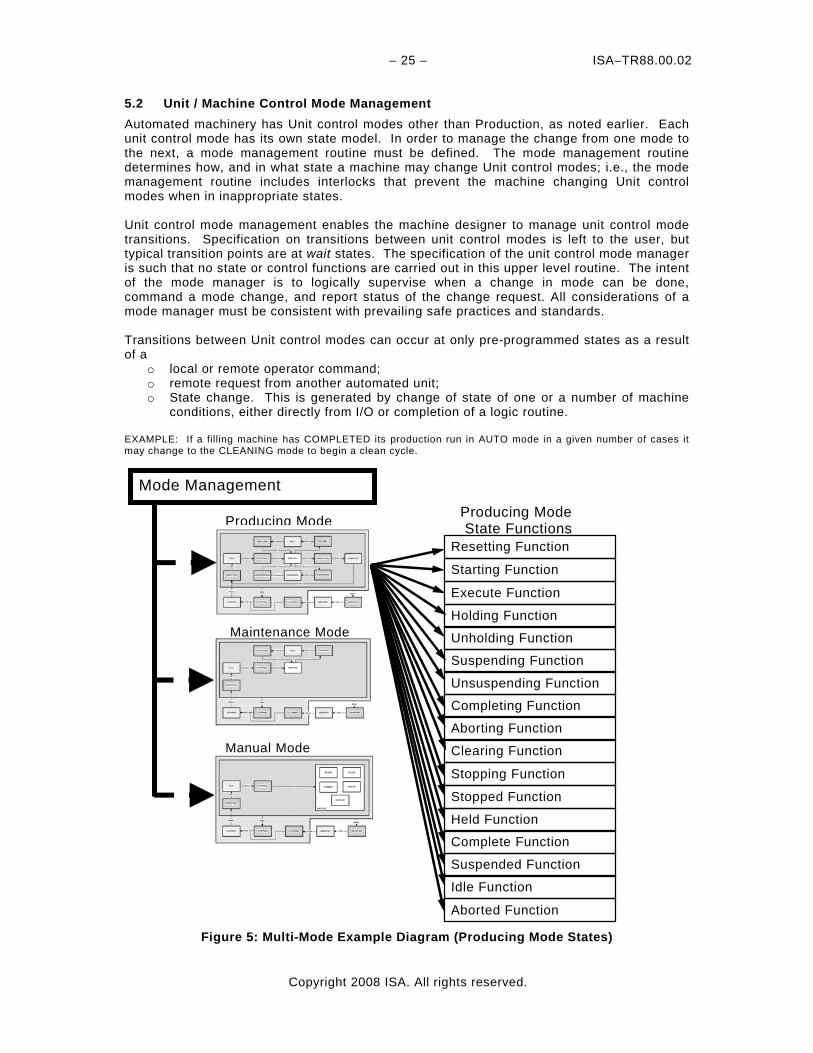
5.2 Unit / Machine Control Mode Management Automated machinery has Unit control modes other than Production, as noted earlier. Each unit control mode has its own state model. In order to manage the change from one mode to the next, a mode management routine must be defined. The mode management routine determines how, and in what state a machine may change Unit control modes; i.e., the mode management routine includes interlocks that prevent the machine changing Unit control modes when in inappropriate states. Unit control mode management enables the machine designer to manage unit control mode transitions. Specification on transitions between unit control modes is left to the user, but typical transition points are at wait states. The specification of the unit control mode manager is such that no state or control functions are carried out in this upper level routine. The intent of the mode manager is to logically supervise when a change in mode can be done, command a mode change, and report status of the change request. All considerations of a mode manager must be consistent with prevailing safe practices and standards. Transitions between Unit control modes can occur at only pre-programmed states as a result of a

o local or remote operator command; o remote request from another automated unit; o State change. This is generated by change of state of one or a number of machine

conditions, either directly from I/O or completion of a logic routine. EXAMPLE: If a filling machine has COMPLETED its production run in AUTO mode in a given number of cases it may change to the CLEANING mode to begin a clean cycle.

Figure 5: Multi-Mode Example Diagram (Producing Mode States)

Mode Management

Producing Mode State Functions

Resetting Function

Starting Function

Aborting Function

Clearing Function

Unsuspending Function

Completing Function

Unholding Function

Suspending Function

Execute Function

Holding Function

Stopping Function

Producing Mode

Maintenance Mode

Manual Mode

Suspended Function

Idle Function

Held Function

Complete Function

Stopped Function

Aborted Function

ISA-TR88.00.02 – 26 –


6 Common Unit/Machine Mode Examples

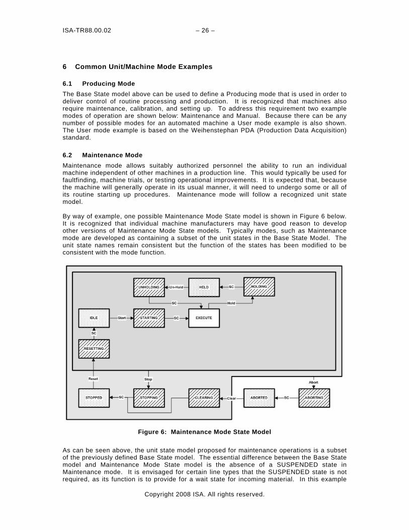
6.1 Producing Mode The Base State model above can be used to define a Producing mode that is used in order to deliver control of routine processing and production. It is recognized that machines also require maintenance, calibration, and setting up. To address this requirement two example modes of operation are shown below: Maintenance and Manual. Because there can be any number of possible modes for an automated machine a User mode example is also shown. The User mode example is based on the Weihenstephan PDA (Production Data Acquisition) standard. 6.2 Maintenance Mode Maintenance mode allows suitably authorized personnel the ability to run an individual machine independent of other machines in a production line. This would typically be used for faultfinding, machine trials, or testing operational improvements. It is expected that, because the machine will generally operate in its usual manner, it will need to undergo some or all of its routine starting up procedures. Maintenance mode will follow a recognized unit state model. By way of example, one possible Maintenance Mode State model is shown in Figure 6 below. It is recognized that individual machine manufacturers may have good reason to develop other versions of Maintenance Mode State models. Typically modes, such as Maintenance mode are developed as containing a subset of the unit states in the Base State Model. The unit state names remain consistent but the function of the states has been modified to be consistent with the mode function.

Figure 6: Maintenance Mode State Model

As can be seen above, the unit state model proposed for maintenance operations is a subset of the previously defined Base State model. The essential difference between the Base State model and Maintenance Mode State model is the absence of a SUSPENDED state in Maintenance mode. It is envisaged for certain line types that the SUSPENDED state is not required, as its function is to provide for a wait state for incoming material. In this example

– 27 – ISA–TR88.00.02


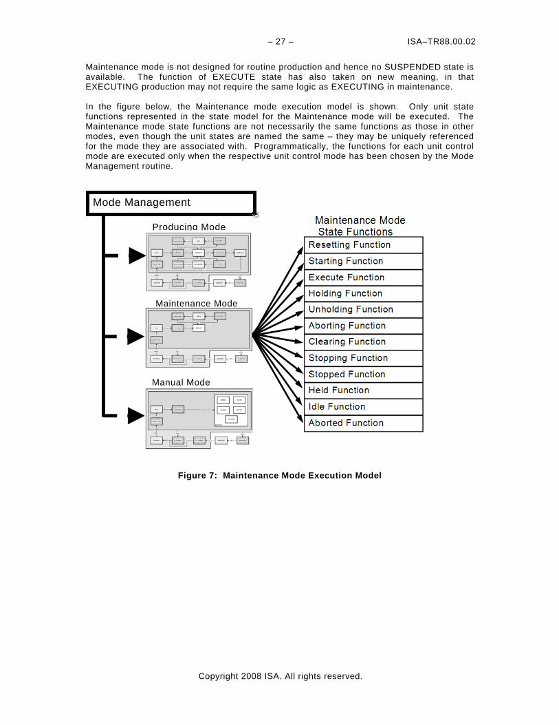
Maintenance mode is not designed for routine production and hence no SUSPENDED state is available. The function of EXECUTE state has also taken on new meaning, in that EXECUTING production may not require the same logic as EXECUTING in maintenance. In the figure below, the Maintenance mode execution model is shown. Only unit state functions represented in the state model for the Maintenance mode will be executed. The Maintenance mode state functions are not necessarily the same functions as those in other modes, even though the unit states are named the same – they may be uniquely referenced for the mode they are associated with. Programmatically, the functions for each unit control mode are executed only when the respective unit control mode has been chosen by the Mode Management routine.

Figure 7: Maintenance Mode Execution Model

Mode Management

Producing Mode

Maintenance Mode

Manual Mode

ISA-TR88.00.02 – 28 –


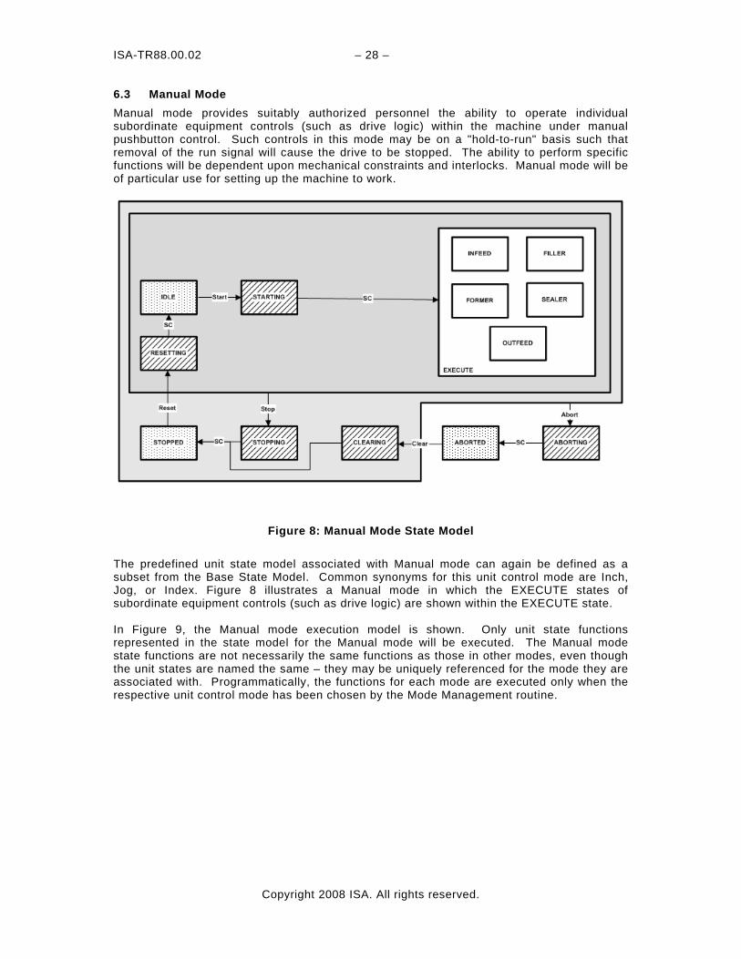
6.3 Manual Mode Manual mode provides suitably authorized personnel the ability to operate individual subordinate equipment controls (such as drive logic) within the machine under manual pushbutton control. Such controls in this mode may be on a "hold-to-run" basis such that removal of the run signal will cause the drive to be stopped. The ability to perform specific functions will be dependent upon mechanical constraints and interlocks. Manual mode will be of particular use for setting up the machine to work.

Figure 8: Manual Mode State Model

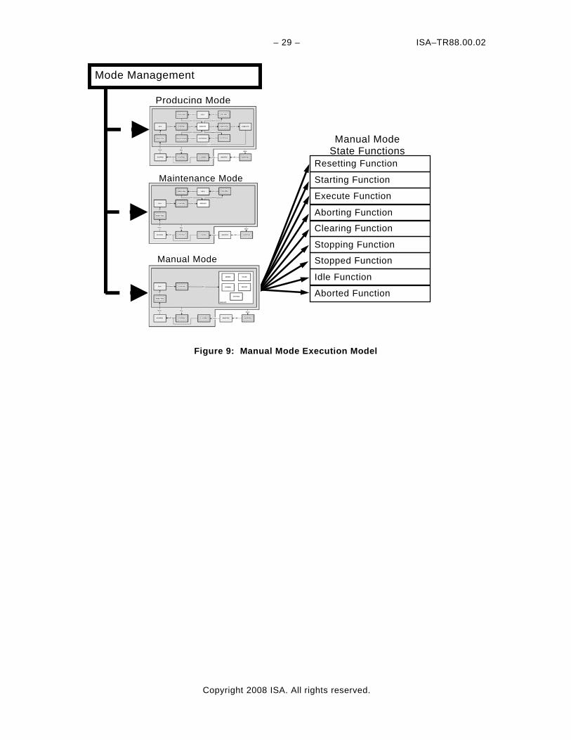
The predefined unit state model associated with Manual mode can again be defined as a subset from the Base State Model. Common synonyms for this unit control mode are Inch, Jog, or Index. Figure 8 illustrates a Manual mode in which the EXECUTE states of subordinate equipment controls (such as drive logic) are shown within the EXECUTE state. In Figure 9, the Manual mode execution model is shown. Only unit state functions represented in the state model for the Manual mode will be executed. The Manual mode state functions are not necessarily the same functions as those in other modes, even though the unit states are named the same – they may be uniquely referenced for the mode they are associated with. Programmatically, the functions for each mode are executed only when the respective unit control mode has been chosen by the Mode Management routine.

– 29 – ISA–TR88.00.02


Figure 9: Manual Mode Execution Model

Mode Management

Producing Mode

Maintenance Mode

Manual Mode

Manual Mode State Functions

Resetting Function

Starting Function

Execute Function

Idle Function

Aborting Function

Clearing Function

Stopping Function

Stopped Function

Aborted Function

ISA-TR88.00.02 – 30 –


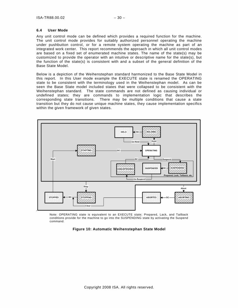
6.4 User Mode Any unit control mode can be defined which provides a required function for the machine. The unit control mode provides for suitably authorized personnel operating the machine under pushbutton control, or for a remote system operating the machine as part of an integrated work center. This report recommends the approach in which all unit control modes are based on a fixed set of enumerated machine states. The name of the state(s) may be customized to provide the operator with an intuitive or descriptive name for the state(s), but the function of the state(s) is consistent with and a subset of the general definition of the Base State Model. Below is a depiction of the Weihenstephan standard harmonized to the Base State Model in this report. In this User mode example the EXECUTE state is renamed the OPERATING state to be consistent with the terminology used in the Weihenstephan model. As can be seen the Base State model included states that were collapsed to be consistent with the Weihenstephan standard. The state commands are not defined as causing individual or undefined states; they are commands to implementation logic that describes the corresponding state transitions. There may be multiple conditions that cause a state transition but they do not cause unique machine states, they cause implementation specifics within the given framework of given states.

Note: OPERATING state is equivalent to an EXECUTE state; Prepared, Lack, and Tailback conditions provide for the machine to go into the SUSPENDING state by activating the Suspend command.

Figure 10: Automatic Weihenstephan State Model

– 31 – ISA–TR88.00.02


7 Automated Machine Functional Tag Description

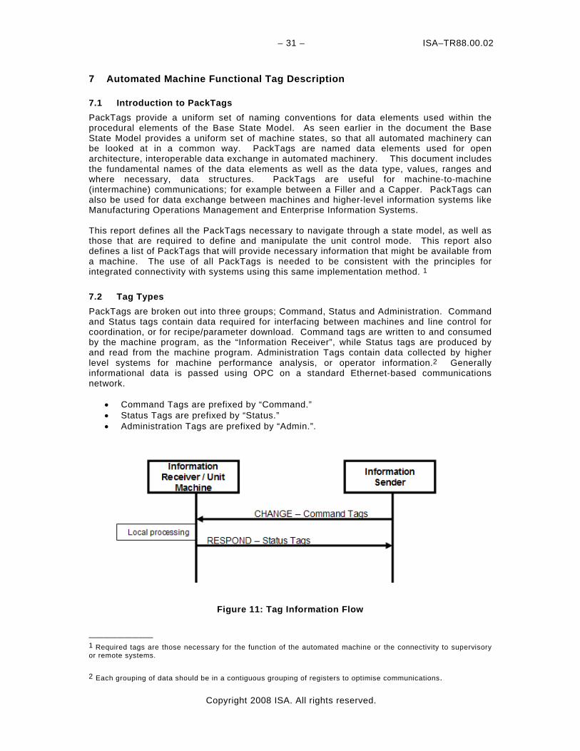
7.1 Introduction to PackTags PackTags provide a uniform set of naming conventions for data elements used within the procedural elements of the Base State Model. As seen earlier in the document the Base State Model provides a uniform set of machine states, so that all automated machinery can be looked at in a common way. PackTags are named data elements used for open architecture, interoperable data exchange in automated machinery. This document includes the fundamental names of the data elements as well as the data type, values, ranges and where necessary, data structures. PackTags are useful for machine-to-machine (intermachine) communications; for example between a Filler and a Capper. PackTags can also be used for data exchange between machines and higher-level information systems like Manufacturing Operations Management and Enterprise Information Systems. This report defines all the PackTags necessary to navigate through a state model, as well as those that are required to define and manipulate the unit control mode. This report also defines a list of PackTags that will provide necessary information that might be available from a machine. The use of all PackTags is needed to be consistent with the principles for integrated connectivity with systems using this same implementation method. 1 7.2 Tag Types PackTags are broken out into three groups; Command, Status and Administration. Command and Status tags contain data required for interfacing between machines and line control for coordination, or for recipe/parameter download. Command tags are written to and consumed by the machine program, as the “Information Receiver”, while Status tags are produced by and read from the machine program. Administration Tags contain data collected by higher level systems for machine performance analysis, or operator information.2 Generally informational data is passed using OPC on a standard Ethernet-based communications network.

• Command Tags are prefixed by “Command.” • Status Tags are prefixed by “Status.” • Administration Tags are prefixed by “Admin.”.

Figure 11: Tag Information Flow

————————— 1 Required tags are those necessary for the function of the automated machine or the connectivity to supervisory or remote systems.

2 Each grouping of data should be in a contiguous grouping of registers to optimise communications.

ISA–TR88.00.02 – 32 –


7.3 PackTags Name Strings In defining tag names, this document uses the common practice of substituting underline characters for spaces between words. Optionally, underscores may also be used in place of the “dot” notation for legacy systems that do not support structured tagnames. The first letter of each word is capitalized for readability. While IEC 61131 is not case sensitive, to ensure inter-operability with all systems it is recommended that the mixed case format be adhered to. Thus, the exact text strings that should be used as tag names should be as follows:

o Status_StateCurrent o Status.StateCurrent

7.4 Data Types, Units, and Ranges The following are the typical data types used for the tags:

o Integer – 32 bit, signed decimal format o Real – 32-bit IEEE 754 standard floating point format (maximum value of 16,777,215

without introducing error in the integer portion of the number) o Binary – Bit pattern o String – null-terminated ASCII, 80 characters default o Time – ISO 8601:1988 24hr Time data type, beginning at 00:00:00. o Date – ISO 8601:1988 Date data type YYYY-MM-DD

7.4.1 Structured Data Types o PACKMLV30 – is a placeholder for the machine unit name, and is the top level in the

PackTag structure. o PMLc – is the collection of all command tags in the PackTag structure. o PMLs – is the collection of all status tags in the PackTag structure. o PMLa – is the collection of all administration tags in the PackTag structure. o Interface – is a collection of tags that are used to describe communication command

values between machines using the PackTag structure. o Descriptor – is a collection of tags that are use to describe parameters in the machine

unit. o Product – is a collection of tags used to describe the product that the machine is

making. o Ingredient – is a collection of tags used to describe the raw materials that are needed

for the product. o Alarm – is the collection tags needed to describe alarm events. o TimeStamp – is the collection of the Time and Date tags.

7.5 Tag Details The following section is a summary listing of the tags. Tag definitions are detailed below:

– 33 – ISA–TR88.00.02


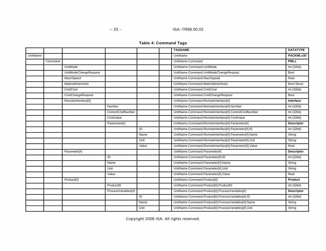
Table 4: Command Tags TAGNAME DATATYPE

UnitName UnitName PACKMLv30

Command UnitName.Command PMLc

UnitMode UnitName.Command.UnitMode Int (32bit)

UnitModeChangeRequest UnitName.Command.UnitModeChangeRequest Bool

MachSpeed UnitName.Command.MachSpeed Real

MaterialInterlocks UnitName.Command.MaterialInterlocks Bool Struct

CntrlCmd UnitName.Command.CntrlCmd Int (32bit)

CmdChangeRequest UnitName.Command.CmdChangeRequest Bool

RemoteInterface[#] UnitName.Command.RemoteInterface[#] Interface

Number UnitName.Command.RemoteInterface[#].Number Int (32bit)

ControlCmdNumber UnitName.Command.RemoteInterface[#].ControlCmdNumber Int (32bit)

CmdValue UnitName.Command.RemoteInterface[#].CmdValue Int (32bit)

Parameter[#] UnitName.Command.RemoteInterface[#].Parameter[#] Descriptor

ID UnitName.Command.RemoteInterface[#].Parameter[#].ID Int (32bit)

Name UnitName.Command.RemoteInterface[#].Parameter[#].Name String

Unit UnitName.Command.RemoteInterface[#].Parameter[#].Unit String

Value UnitName.Command.RemoteInterface[#].Parameter[#].Value Real

Parameter[#] UnitName.Command.Parameter[#] Descriptor

ID UnitName.Command.Parameter[#].ID Int (32bit)

Name UnitName.Command.Parameter[#].Name String

Unit UnitName.Command.Parameter[#].Unit String

Value UnitName.Command.Parameter[#].Value Real

Product[#] UnitName.Command.Product[#] Product

ProductID UnitName.Command.Product[#].ProductID Int (32bit)

ProcessVariables[#] UnitName.Command.Product[#].ProcessVariables[#] Descriptor

ID UnitName.Command.Product[#].ProcessVariables[#].ID Int (32bit)

Name UnitName.Command.Product[#].ProcessVariables[#].Name String

Unit UnitName.Command.Product[#].ProcessVariables[#].Unit String

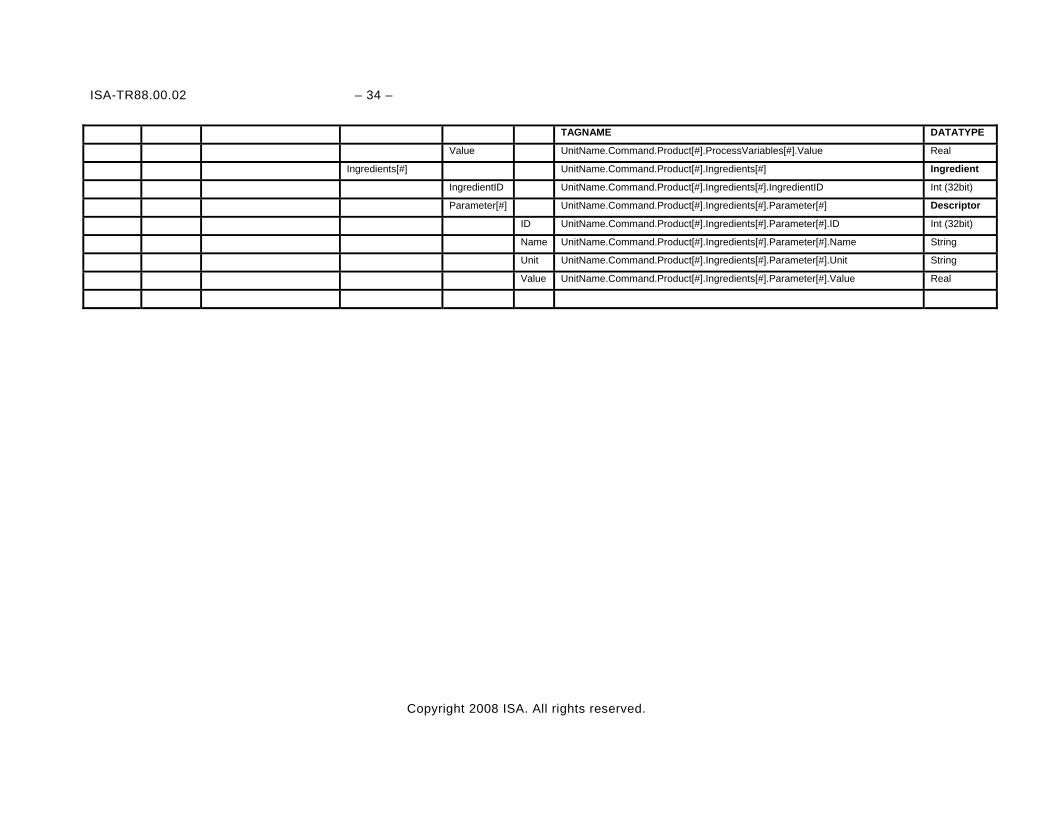
ISA-TR88.00.02 – 34 –


TAGNAME DATATYPE

Value UnitName.Command.Product[#].ProcessVariables[#].Value Real

Ingredients[#] UnitName.Command.Product[#].Ingredients[#] Ingredient

IngredientID UnitName.Command.Product[#].Ingredients[#].IngredientID Int (32bit)

Parameter[#] UnitName.Command.Product[#].Ingredients[#].Parameter[#] Descriptor

ID UnitName.Command.Product[#].Ingredients[#].Parameter[#].ID Int (32bit)

Name UnitName.Command.Product[#].Ingredients[#].Parameter[#].Name String

Unit UnitName.Command.Product[#].Ingredients[#].Parameter[#].Unit String

Value UnitName.Command.Product[#].Ingredients[#].Parameter[#].Value Real

– 35 – ISA–TR88.00.02


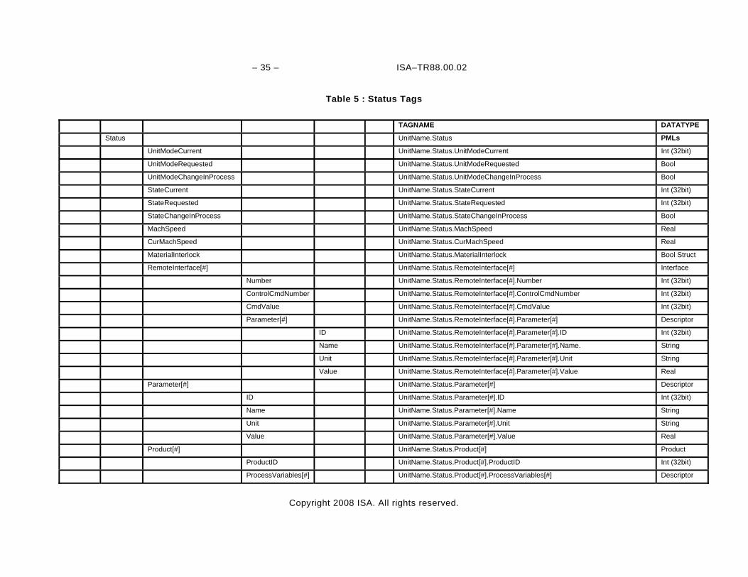
Table 5 : Status Tags

TAGNAME DATATYPE

Status UnitName.Status PMLs

UnitModeCurrent UnitName.Status.UnitModeCurrent Int (32bit)

UnitModeRequested UnitName.Status.UnitModeRequested Bool

UnitModeChangeInProcess UnitName.Status.UnitModeChangeInProcess Bool

StateCurrent UnitName.Status.StateCurrent Int (32bit)

StateRequested UnitName.Status.StateRequested Int (32bit)

StateChangeInProcess UnitName.Status.StateChangeInProcess Bool

MachSpeed UnitName.Status.MachSpeed Real

CurMachSpeed UnitName.Status.CurMachSpeed Real

MaterialInterlock UnitName.Status.MaterialInterlock Bool Struct

RemoteInterface[#] UnitName.Status.RemoteInterface[#] Interface

Number UnitName.Status.RemoteInterface[#].Number Int (32bit)

ControlCmdNumber UnitName.Status.RemoteInterface[#].ControlCmdNumber Int (32bit)

CmdValue UnitName.Status.RemoteInterface[#].CmdValue Int (32bit)

Parameter[#] UnitName.Status.RemoteInterface[#].Parameter[#] Descriptor

ID UnitName.Status.RemoteInterface[#].Parameter[#].ID Int (32bit)

Name UnitName.Status.RemoteInterface[#].Parameter[#].Name. String

Unit UnitName.Status.RemoteInterface[#].Parameter[#].Unit String

Value UnitName.Status.RemoteInterface[#].Parameter[#].Value Real

Parameter[#] UnitName.Status.Parameter[#] Descriptor

ID UnitName.Status.Parameter[#].ID Int (32bit)

Name UnitName.Status.Parameter[#].Name String

Unit UnitName.Status.Parameter[#].Unit String

Value UnitName.Status.Parameter[#].Value Real

Product[#] UnitName.Status.Product[#] Product

ProductID UnitName.Status.Product[#].ProductID Int (32bit)

ProcessVariables[#] UnitName.Status.Product[#].ProcessVariables[#] Descriptor

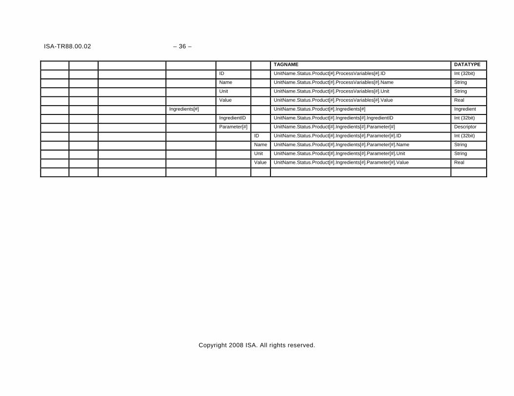
ISA-TR88.00.02 – 36 –


TAGNAME DATATYPE

ID UnitName.Status.Product[#].ProcessVariables[#].ID Int (32bit)

Name UnitName.Status.Product[#].ProcessVariables[#].Name String

Unit UnitName.Status.Product[#].ProcessVariables[#].Unit String

Value UnitName.Status.Product[#].ProcessVariables[#].Value Real

Ingredients[#] UnitName.Status.Product[#].Ingredients[#] Ingredient

IngredientID UnitName.Status.Product[#].Ingredients[#].IngredientID Int (32bit)

Parameter[#] UnitName.Status.Product[#].Ingredients[#].Parameter[#] Descriptor

ID UnitName.Status.Product[#].Ingredients[#].Parameter[#].ID Int (32bit)

Name UnitName.Status.Product[#].Ingredients[#].Parameter[#].Name String

Unit UnitName.Status.Product[#].Ingredients[#].Parameter[#].Unit String

Value UnitName.Status.Product[#].Ingredients[#].Parameter[#].Value Real

– 37 – ISA–TR88.00.02


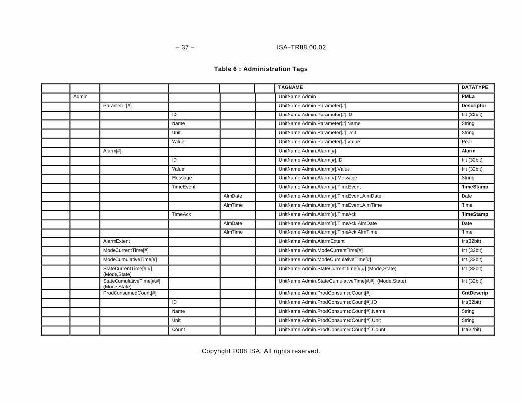
Table 6 : Administration Tags

TAGNAME DATATYPE

Admin UnitName.Admin PMLa

Parameter[#] UnitName.Admin.Parameter[#] Descriptor

ID UnitName.Admin.Parameter[#].ID Int (32bit)

Name UnitName.Admin.Parameter[#].Name String

Unit UnitName.Admin.Parameter[#].Unit String

Value UnitName.Admin.Parameter[#].Value Real

Alarm[#] UnitName.Admin.Alarm[#] Alarm

ID UnitName.Admin.Alarm[#].ID Int (32bit)

Value UnitName.Admin.Alarm[#].Value Int (32bit)

Message UnitName.Admin.Alarm[#].Message String

TimeEvent UnitName.Admin.Alarm[#].TimeEvent TimeStamp

AlmDate UnitName.Admin.Alarm[#].TimeEvent.AlmDate Date

AlmTime UnitName.Admin.Alarm[#].TimeEvent.AlmTime Time

TimeAck UnitName.Admin.Alarm[#].TimeAck TimeStamp

AlmDate UnitName.Admin.Alarm[#].TimeAck.AlmDate Date

AlmTime UnitName.Admin.Alarm[#].TimeAck.AlmTime Time

AlarmExtent UnitName.Admin.AlarmExtent Int(32bit)

ModeCurrentTime[#] UnitName.Admin.ModeCurrentTime[#] Int (32bit)

ModeCumulativeTime[#] UnitName.Admin.ModeCumulativeTime[#] Int (32bit)

StateCurrentTime[#,#] (Mode,State)

UnitName.Admin.StateCurrentTime[#,#] (Mode,State) Int (32bit)

StateCumulativeTime[#,#] (Mode,State)

UnitName.Admin.StateCumulativeTime[#,#] (Mode,State) Int (32bit)

ProdConsumedCount[#] UnitName.Admin.ProdConsumedCount[#] CntDescrip

ID UnitName.Admin.ProdConsumedCount[#].ID Int(32bit)

Name UnitName.Admin.ProdConsumedCount[#].Name String

Unit UnitName.Admin.ProdConsumedCount[#].Unit String

Count UnitName.Admin.ProdConsumedCount[#].Count Int(32bit)

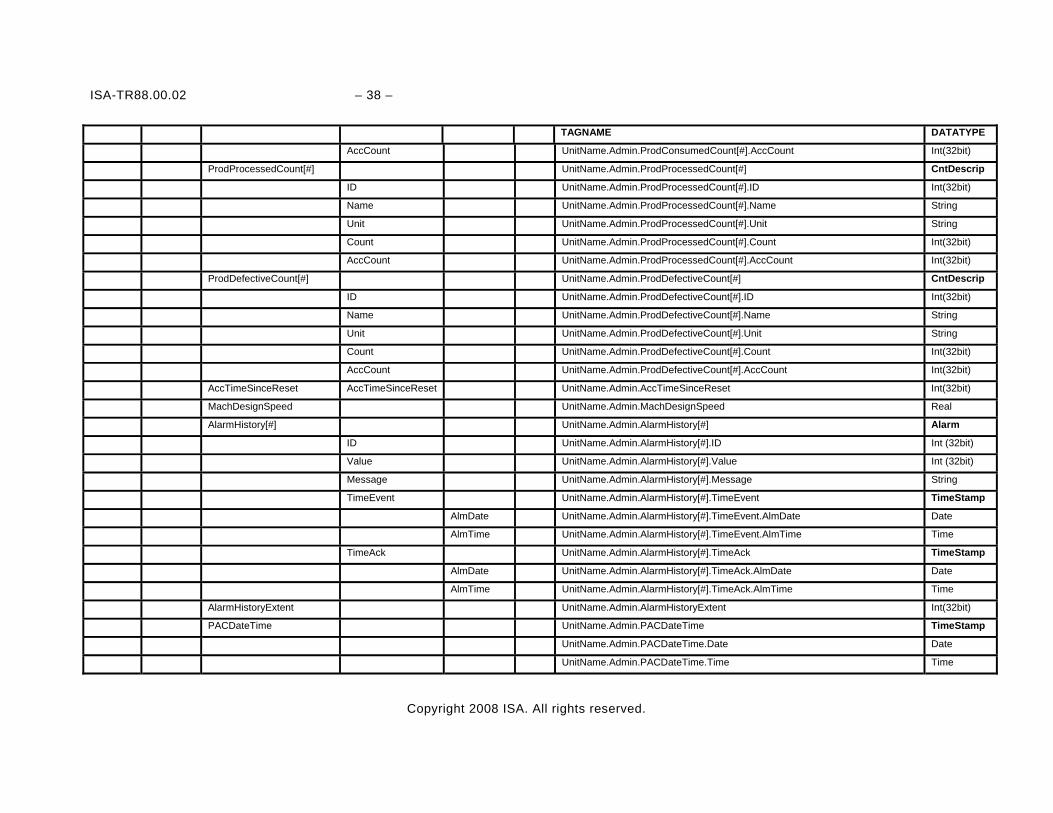
ISA-TR88.00.02 – 38 –


TAGNAME DATATYPE

AccCount UnitName.Admin.ProdConsumedCount[#].AccCount Int(32bit)

ProdProcessedCount[#] UnitName.Admin.ProdProcessedCount[#] CntDescrip

ID UnitName.Admin.ProdProcessedCount[#].ID Int(32bit)

Name UnitName.Admin.ProdProcessedCount[#].Name String

Unit UnitName.Admin.ProdProcessedCount[#].Unit String

Count UnitName.Admin.ProdProcessedCount[#].Count Int(32bit)

AccCount UnitName.Admin.ProdProcessedCount[#].AccCount Int(32bit)

ProdDefectiveCount[#] UnitName.Admin.ProdDefectiveCount[#] CntDescrip

ID UnitName.Admin.ProdDefectiveCount[#].ID Int(32bit)

Name UnitName.Admin.ProdDefectiveCount[#].Name String

Unit UnitName.Admin.ProdDefectiveCount[#].Unit String

Count UnitName.Admin.ProdDefectiveCount[#].Count Int(32bit)

AccCount UnitName.Admin.ProdDefectiveCount[#].AccCount Int(32bit)

AccTimeSinceReset AccTimeSinceReset UnitName.Admin.AccTimeSinceReset Int(32bit)

MachDesignSpeed UnitName.Admin.MachDesignSpeed Real

AlarmHistory[#] UnitName.Admin.AlarmHistory[#] Alarm

ID UnitName.Admin.AlarmHistory[#].ID Int (32bit)

Value UnitName.Admin.AlarmHistory[#].Value Int (32bit)

Message UnitName.Admin.AlarmHistory[#].Message String

TimeEvent UnitName.Admin.AlarmHistory[#].TimeEvent TimeStamp

AlmDate UnitName.Admin.AlarmHistory[#].TimeEvent.AlmDate Date

AlmTime UnitName.Admin.AlarmHistory[#].TimeEvent.AlmTime Time

TimeAck UnitName.Admin.AlarmHistory[#].TimeAck TimeStamp

AlmDate UnitName.Admin.AlarmHistory[#].TimeAck.AlmDate Date

AlmTime UnitName.Admin.AlarmHistory[#].TimeAck.AlmTime Time

AlarmHistoryExtent UnitName.Admin.AlarmHistoryExtent Int(32bit)

PACDateTime UnitName.Admin.PACDateTime TimeStamp

UnitName.Admin.PACDateTime.Date Date

UnitName.Admin.PACDateTime.Time Time

ISA–TR88.00.02 – 39 –


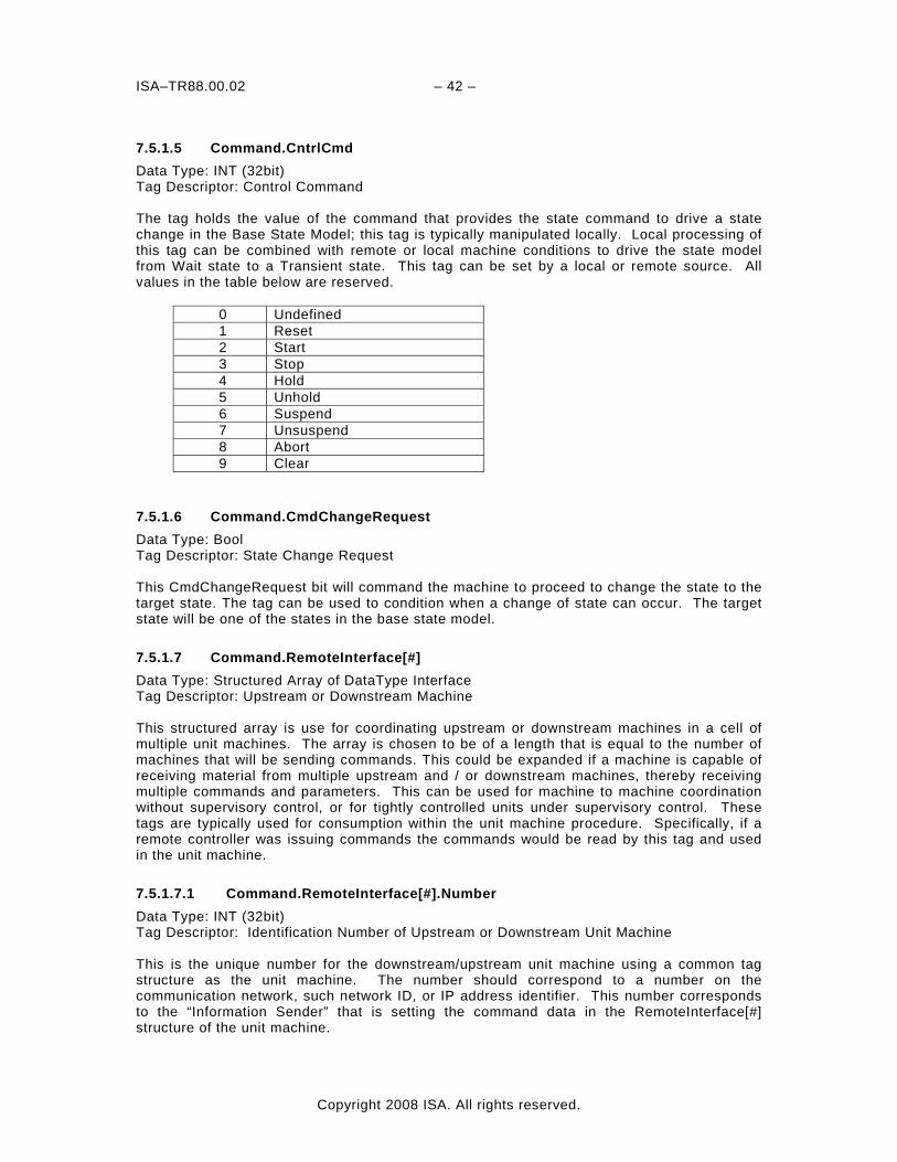
7.5.1 Command Tags Command tags are used to control the operation of the unit machine. Command tags include unit state commands which control the state transitions in the Base State Model. The command tags also include parameters and process variables which control how the machine operates. Command tags generally originate from the machine user or a remote system. The originator of the command in this report is defined as the “requestor” or “information sender.” The unit machine in this report is known as the “execution system”. 7.5.1.1 Command.UnitMode Data Type: INT (32bit) Tag Descriptor: Unit Mode Target This value is predefined by the user/OEM, and are the desired unit modes of the machine. The UnitMode tag is a numerical representation of the commanded mode. There can be any number of unit modes, and for each unit mode there is an accompanying state model. EXAMPLE: Unit modes are Production, Maintenance, Manual, Clean Out, Dry Run, Setup, etc.

0 Undefined 1 Producing 2 Maintenance 3 Manual 4 <future reserve> 5 <future reserve> 6 <future reserve> 7 <future reserve> 8 <future reserve> 9 <future reserve> 10 <future reserve> 11 <future reserve> 12 <future reserve> 13 <future reserve> 14 <future reserve> 15 <future reserve> 16 User Defined 1 17 User Defined 2 N User Defined n

7.5.1.2 Command.UnitModeChangeRequest Data Type: Bool Tag Descriptor: Request Unit Mode Change When a unit mode request takes place a numerical value must be present in the Command.UnitMode tag to change the unit mode. Local processing and conditioning of the requested mode change is necessary in order to accept, reject, or condition the timing of the change request.

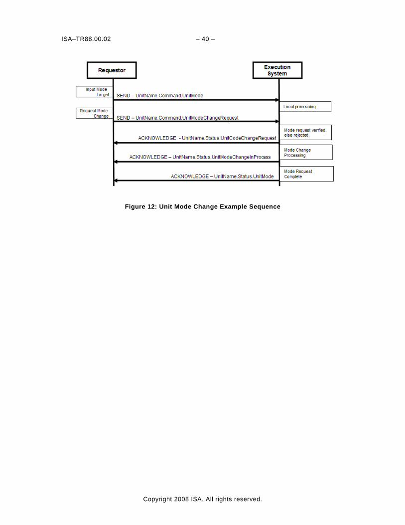
ISA–TR88.00.02 – 40 –


Figure 12: Unit Mode Change Example Sequence

– 41 – ISA–TR88.00.02


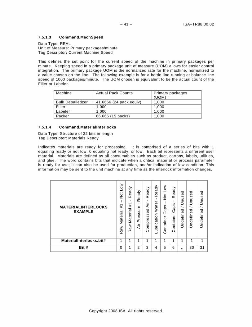
7.5.1.3 Command.MachSpeed Data Type: REAL Unit of Measure: Primary packages/minute Tag Descriptor: Current Machine Speed This defines the set point for the current speed of the machine in primary packages per minute. Keeping speed in a primary package unit of measure (UOM) allows for easier control integration. The primary package UOM is the normalized rate for the machine, normalized to a value chosen on the line. The following example is for a bottle line running at balance line speed of 1000 packages/minute. The UOM chosen is equivalent to be the actual count of the Filler or Labeler.

Machine Actual Pack Counts Primary packages (UOM)

Bulk Depalletizer 41.6666 (24 pack equiv) 1,000 Filler 1,000 1,000 Labeler 1,000 1,000 Packer 66.666 (15 packs) 1,000

7.5.1.4 Command.MaterialInterlocks Data Type: Structure of 32 bits in length Tag Descriptor: Materials Ready Indicates materials are ready for processing. It is comprised of a series of bits with 1 equaling ready or not low, 0 equaling not ready, or low. Each bit represents a different user material. Materials are defined as all consumables such as product, cartons, labels, utilities, and glue. The word contains bits that indicate when a critical material or process parameter is ready for use; it can also be used for production, and/or indication of low condition. This information may be sent to the unit machine at any time as the interlock information changes.

MATERIALINTERLOCKS EXAMPLE

Raw

Mat

eria

l #1

– N

ot L

ow

Raw

Mat

eria

l #1

- R

eady

Air

Pre

ssur

e -

Rea

dy

Com

pres

sed

Air

- R

eady

Lubr

icat

ion

Wat

er -

Rea

dy

Con

tain

er C

aps

– N

ot L

ow

Con

tain

er C

aps

– R

eady

Und

efin

ed /

Unu

sed

Und

efin

ed /

Unu

sed

Und

efin

ed /

Unu

sed

MaterialInterlocks.bit# 1 1 1 1 1 1 1 1 1 1

Bit # 0 1 2 3 4 5 6 .. 30 31

ISA–TR88.00.02 – 42 –


7.5.1.5 Command.CntrlCmd Data Type: INT (32bit) Tag Descriptor: Control Command The tag holds the value of the command that provides the state command to drive a state change in the Base State Model; this tag is typically manipulated locally. Local processing of this tag can be combined with remote or local machine conditions to drive the state model from Wait state to a Transient state. This tag can be set by a local or remote source. All values in the table below are reserved.

0 Undefined 1 Reset 2 Start 3 Stop 4 Hold 5 Unhold 6 Suspend 7 Unsuspend 8 Abort 9 Clear

7.5.1.6 Command.CmdChangeRequest Data Type: Bool Tag Descriptor: State Change Request This CmdChangeRequest bit will command the machine to proceed to change the state to the target state. The tag can be used to condition when a change of state can occur. The target state will be one of the states in the base state model. 7.5.1.7 Command.RemoteInterface[#] Data Type: Structured Array of DataType Interface Tag Descriptor: Upstream or Downstream Machine This structured array is use for coordinating upstream or downstream machines in a cell of multiple unit machines. The array is chosen to be of a length that is equal to the number of machines that will be sending commands. This could be expanded if a machine is capable of receiving material from multiple upstream and / or downstream machines, thereby receiving multiple commands and parameters. This can be used for machine to machine coordination without supervisory control, or for tightly controlled units under supervisory control. These tags are typically used for consumption within the unit machine procedure. Specifically, if a remote controller was issuing commands the commands would be read by this tag and used in the unit machine. 7.5.1.7.1 Command.RemoteInterface[#].Number Data Type: INT (32bit) Tag Descriptor: Identification Number of Upstream or Downstream Unit Machine This is the unique number for the downstream/upstream unit machine using a common tag structure as the unit machine. The number should correspond to a number on the communication network, such network ID, or IP address identifier. This number corresponds to the “Information Sender” that is setting the command data in the RemoteInterface[#] structure of the unit machine.

– 43 – ISA–TR88.00.02


7.5.1.7.2 Command.RemoteInterface[#].ControlCmdNumber Data Type: INT (32bit) Tag Descriptor : Control Command for Upstream or Downstream Machine A user defined command number associated with coded value from a remote unit. This number is a coded value sent from one node on the network to another. The value can be associated with a unit mode change request, speed change request, a state change request, etc. 7.5.1.7.3 Command.RemoteInterface[#].CmdValue Data Type: INT (32bit) Tag Descriptor: Control Command Value Associated ControlCmdNumber This is the command value associated with the ControlCmdNumber above. The command value may be the speed requested, state change, etc. EXAMPLE: For an upstream machine designated as #2 a control command number of 5 may be related to the speed setting value for the machine. A value of 400 can be used to modify the remote machine setpoint. Command.RemoteInterface[1].Number = 2 Command.RemoteInterface[1].ControlCmdNumber = 5 Command.RemoteInterface[1].CmdValue = 400 For a downstream machine designated as #4 the control command number of 0 can be used to remotely command a state transition for the machine. The value of 2 is the command value for start. Command.RemoteInterface[1].Number = 4 Command.RemoteInterface[1].ControlCmdNumber = 0 Command.RemoteInterface[1].CmdValue = 2 7.5.1.7.4 Command.RemoteInterface[#].Parameter[#] Data Type: Structured Array of Data Type Descriptor The Parameter tags associated to Commanded Remote Interface are typically used for command parameters that are given to the unit machine from remote machines. The parameters are typically needed for coordinating the unit machine or production with other machines. The parameter value may be anything from machine limit parameters to temperatures and counter presets. The parameters are typically limited to machine parameters as product and process parameters are describe in later tags. 7.5.1.7.4.1 Command. RemoteInterface[#].Parameter[#].ID Data Type: INT (32bit) Tag Descriptor: ID Value of Parameter This is the arbitrary (user defined) ID value assigned to the parameter. This is non-descript value that can be used for user tag requirements. 7.5.1.7.4.2 Command.RemoteInterface[#].Parameter[#].Name Data Type: String Tag Descriptor: String value assigned to Parameter The literal parameter name is used to describe the parameter variable number, and its associated value from the remote interface. An example parameter name may be GLUE TEMP, BEARING TEMP, OVERLOAD TIME, etc. 7.5.1.7.4.3 Command.RemoteInterface[#].Parameter[#].Unit Data Type: String[5] Tag Descriptor:String value of Parameter unit of measure

ISA–TR88.00.02 – 44 –


Unit is a string that describes the unit of measure associated with the parameter’s value (i.e., secs, deg, rpm, ppm, etc). This tag describes the unit of measure associated with the following tag value sent from the remote interface. 7.5.1.7.4.4 Command.RemoteInterface[#].Parameter[#].Value Data Type: REAL Tag Descriptor: Numeric Value of Parameter This is the numeric value of the parameter. The value is described by the Parameter[#].ID, Parameter[#].Name, and is of unit of measure is described by the Parameter[#].Unit sent by the remote interface as a command to the unit machine. 7.5.1.8 Command.Parameter[#] Data Type: Array of Data Type Descriptor The Parameter tags associated to the local Interface and are typically used for command parameters that are given to the unit locally, for example from an HMI. The parameters are typically needed for running the unit machine. The parameter value may be anything from machine limit parameters to temperatures and counter presets. The parameters are typically limited to machine parameters as product and process parameters are describe in later tags. 7.5.1.8.1 Command.Parameter[#].ID Data Type: INT (32bit) Tag Descriptor: ID value of Parameter This is the arbitrary (user defined) ID value of the parameter. This is non-descript value that can be used for any user tag requirements. 7.5.1.8.2 Command.Parameter[#].Name Data Type: STRING Tag Descriptor: Structured array of Parameter names for the machine unit. The literal parameter name is used to describe the parameter number, and its associated value. An example parameter name may be GLUE TEMP, BEARING TEMP, OVERLOAD TIME, etc. 7.5.1.8.3 Command.Parameter[#].Unit Data Type: STRING[5] Tag Descriptor: Structured Array of Parameter Unit of Measure for the Machine Unit The parameter unit is used to describe the unit of measure of the parameter, and its associated value. An example parameter unit of measure may be DegF, secs, PPM, revs, mm, etc. 7.5.1.8.4 Command.Parameter[#].Value Data Type: Real Tag Descriptor: Structured Array of Parameter Values This is the numeric value of the parameter. The value is described by the Parameter[#].ID, Parameter[#].Name, and is a unit of measure described by the Parameter[#].Unit commanded by the local interface, or local processor, as a command to the unit machine. EXAMPLE: Command.Parameter[1].Value = 22.5 Command.Parameter[2].Value = 12

– 45 – ISA–TR88.00.02


EXAMPLE: Machine Unit Process Variable Command.Parameter[1].Name = BEARING_1_OVERTEMP Command.Parameter[1].Unit = DegC Command.Parameter[1].Value = 350.00 This defines the temperature of a Bearing Overtemp alarm of the #1 bearing is to be set at 350.0 Degrees C for all products.

ISA–TR88.00.02 – 46 –


7.5.1.9 Command.Product[#] Data Type: Array of Data Type Product The Product data type can be used for defining product and product processing parameter variables. The command tags can come from either a local HMI or remote systems and are used to process the product on the unit machine. The array is typically needed for machines that run multiple products. 7.5.1.9.1 Command.Product[#].ProductID Data Type: INT (32bit) Tag Descriptor: Structured Array of Product ID# This Product ID is used to indicate to the machine which product it is producing (i.e., SKU or UPC). The array can be used for machines that run multiple products. 7.5.1.9.2 Command.Product[#].ProcessVariables[#] Data Type: Array of Data Type Descriptor The Process Variables structured array can be used for specific process variables needed by the unit machine for the processing of a specific product. Process variables include set points, limits, quality parameters, etc, that are needed to produce a particular product on a unit machine. The number of tags for this array will be the maximum number of needed process variables for any particular product defined on the unit machine. 7.5.1.9.2.1 Command.Product[#].ProcessVariables[#].ID Data Type: INT (32bit) Tag Descriptor: ID Value of Parameter This is the arbitrary (user defined) process variable ID value assigned to the process variable. 7.5.1.9.2.2 Command.Product[#].ProcessVariables[#].Name Data Type: STRING Tag Descriptor: Structured Array of Process Variable Names for Multiple Product ID#s The process variable literal name is used to describe the process variable number, and its associated value. An example process variable name may be GLUE TEMP, MaxTimeInMachine, MixingTime, KnifeSpeed, ChillRollPhaseOffset, etc. 7.5.1.9.2.3 Command.Product[#].ProcessVariables[#].Unit Data Type: STRING[5] Tag Descriptor: Structured Array of Process Variable Unit of Measure The process variable unit of measure is a string data type used to describe the unit of measure of the process variable number, and its associated value. An example process unit of measure may be DegF, secs, PPM, revs, mm, etc. . 7.5.1.9.2.4 Command.Product[#].ProcessVariables[#].Value Data Type: Real Tag Descriptor: Structured Array of Process Variable Values The process variable value is used to specify a process variable for the Product[#] specified by the ProcessVariable[#].ID, ProcessVariables[#].Name, and ProcessVariables[#].Unit. Command.Product[1].ProcessVariables[1].Value = 22.5

– 47 – ISA–TR88.00.02


Command.Product[1].ProcessVariables[2].Value = 12 Combined with other examples of Product[#] Command.Product[1].ProcessVariables[1].Name = Glue1Temp Command.Product[1].ProcessVariables[1].Unit = DegF Command.Product[1].ProcessVariables[1].Value = 356.4 Meaning the temperature of at Glue station 1 is to be controlled at 356.4 Degrees F for product number 1. Other Examples of Process Variable Name for Products: Name = ProductMaxTimeInMachine Name = ProductMinTimeInMachine Name = ByproductID Name = ByproductsMaxTimeInMachine

ISA–TR88.00.02 – 48 –


7.5.1.9.3 Command.Product[#].Ingredients[#] Data Type: Array of Data Type Ingredient This array serves to hold the information needed for the raw materials that are used by the unit machine in the processing of a particular product. The extent of this array will be the maximum number of ingredients used in the processing of any particular product. 7.5.1.9.3.1 Command.Product[#].Ingredients[#].IngredientID Data Type: INT (32bit) Tag Descriptor: Structured Array of Ingredient IDs The Ingredient ID is an arbitrary number associated with the raw material, or ingredient for a particular product number. The user will define the value associated to the ingredient IDs that are used in the operation of the machine for a particular product. Each ingredient should have a distinct ID (SKU or UPC). 7.5.1.9.3.2 Command.Product[#].Ingredients[#].Parameter[#] Data Type: Array of Data Type Descriptor This array or structures is used for parameters associated with a particular ingredient or raw material used the processing of a particular product number. This command tag is typically set by a “Information Sender” to the unit machine controller. The extent of this array is the maximum number of parameters associated with any ingredient in any product that is defined on the unit machine. 7.5.1.9.3.2.1 Command.Product[#].Ingredients[#].Parameter[#].ID Data Type: INT (32bit) Tag Descriptor: ID Value of Parameter This is the arbitrary (user defined) ID value assigned to one of the parameters for the ingredient or raw material, needed for the processing of the product defined by the product number. 7.5.1.9.3.2.2 Command.Product[#].Ingredients[#].Parameter[#].Name Data Type: STRING Tag Descriptor: Structured Array of Ingredient Parameter Names The parameter variable name in the parameter array is used to describe the parameter names associated with a specific ingredient number in a specific product number. An example parameter name may be SETUP TIME, TEMP, TAB POSITION etc. The array is typically needed for machines that run multiple ingredients with multiple parameters with multiple products. 7.5.1.9.3.2.3 Command.Product[#].Ingredients[#].Parameter[#].Unit Data Type: STRING[5] Tag Descriptor: Structured Array of Unit of Measure The parameter unit tag is used to describe the parameter names associated with a specific parameter in an specific ingredient in a specific product. An example unit of measure name may be DegF, secs, PPM, revs, mm, etc. The array is typically needed for unit machines that run multiple products with multiple ingredients with multiple processing parameters. 7.5.1.9.3.2.4 Command.Product[#].Ingredients[#].Parameter[#].Value Data Type: Real Tag Descriptor: Structured Array of Values

– 49 – ISA–TR88.00.02


The ingredient parameter value is used to specify a parameter variable for the control of the process. The array is typically needed for unit machines that run multiple products with multiple ingredients with multiple processing parameters. As an example with Ingredient number 1 in Product number 1: Command.Product[1].Ingredients[1].Parameter[1].Value = 225 Command.Product[1].Ingredients[1].Parameter[2].Value = 12 Combined with other examples of Product[#] Command.Product[1].Ingredients[1].Parameter[1].Name = KNIFE_OFFSET Command.Product[1].Ingredients[1].Parameter[1].Unit = degrees Command.Product[1].Ingredients[1].Parameter[1].Value = 3.564 Meaning the offset of the knife is to be controlled at 3.564 Degrees for Parameter variable number 1, on ingredient 1 for product number 1.

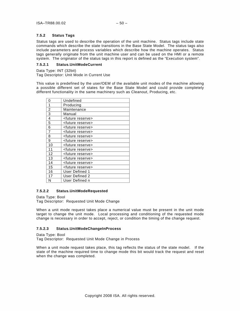
ISA–TR88.00.02 – 50 –


7.5.2 Status Tags Status tags are used to describe the operation of the unit machine. Status tags include state commands which describe the state transitions in the Base State Model. The status tags also include parameters and process variables which describe how the machine operates. Status tags generally originate from the unit machine user and can be used on the HMI or a remote system. The originator of the status tags in this report is defined as the “Execution system”. 7.5.2.1 Status.UnitModeCurrent Data Type: INT (32bit) Tag Descriptor: Unit Mode in Current Use This value is predefined by the user/OEM of the available unit modes of the machine allowing a possible different set of states for the Base State Model and could provide completely different functionality in the same machinery such as Cleanout, Producing, etc.

0 Undefined 1 Producing 2 Maintenance 3 Manual 4 <future reserve> 5 <future reserve> 6 <future reserve> 7 <future reserve> 8 <future reserve> 9 <future reserve> 10 <future reserve> 11 <future reserve> 12 <future reserve> 13 <future reserve> 14 <future reserve> 15 <future reserve> 16 User Defined 1 17 User Defined 2 N User Defined n

7.5.2.2 Status.UnitModeRequested Data Type: Bool Tag Descriptor: Requested Unit Mode Change When a unit mode request takes place a numerical value must be present in the unit mode target to change the unit mode. Local processing and conditioning of the requested mode change is necessary in order to accept, reject, or condition the timing of the change request. 7.5.2.3 Status.UnitModeChangeInProcess Data Type: Bool Tag Descriptor: Requested Unit Mode Change in Process When a unit mode request takes place, this tag reflects the status of the state model. If the state of the machine required time to change mode this bit would track the request and reset when the change was completed.

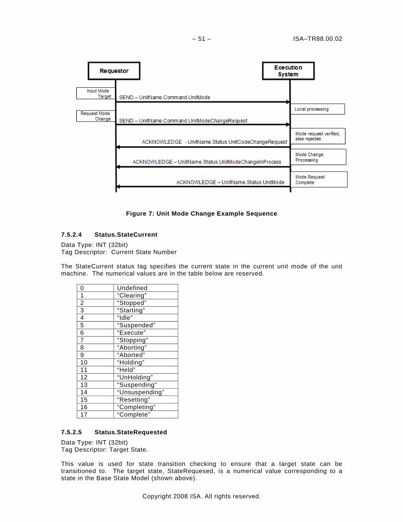
– 51 – ISA–TR88.00.02


Figure 7: Unit Mode Change Example Sequence

7.5.2.4 Status.StateCurrent Data Type: INT (32bit) Tag Descriptor: Current State Number The StateCurrent status tag specifies the current state in the current unit mode of the unit machine. The numerical values are in the table below are reserved.

0 Undefined 1 “Clearing” 2 “Stopped” 3 “Starting” 4 “Idle” 5 “Suspended” 6 “Execute” 7 “Stopping” 8 “Aborting” 9 “Aborted” 10 “Holding” 11 “Held” 12 “UnHolding” 13 “Suspending” 14 “Unsuspending” 15 “Resetting” 16 “Completing” 17 “Complete”

7.5.2.5 Status.StateRequested Data Type: INT (32bit) Tag Descriptor: Target State. This value is used for state transition checking to ensure that a target state can be transitioned to. The target state, StateRequesed, is a numerical value corresponding to a state in the Base State Model (shown above).

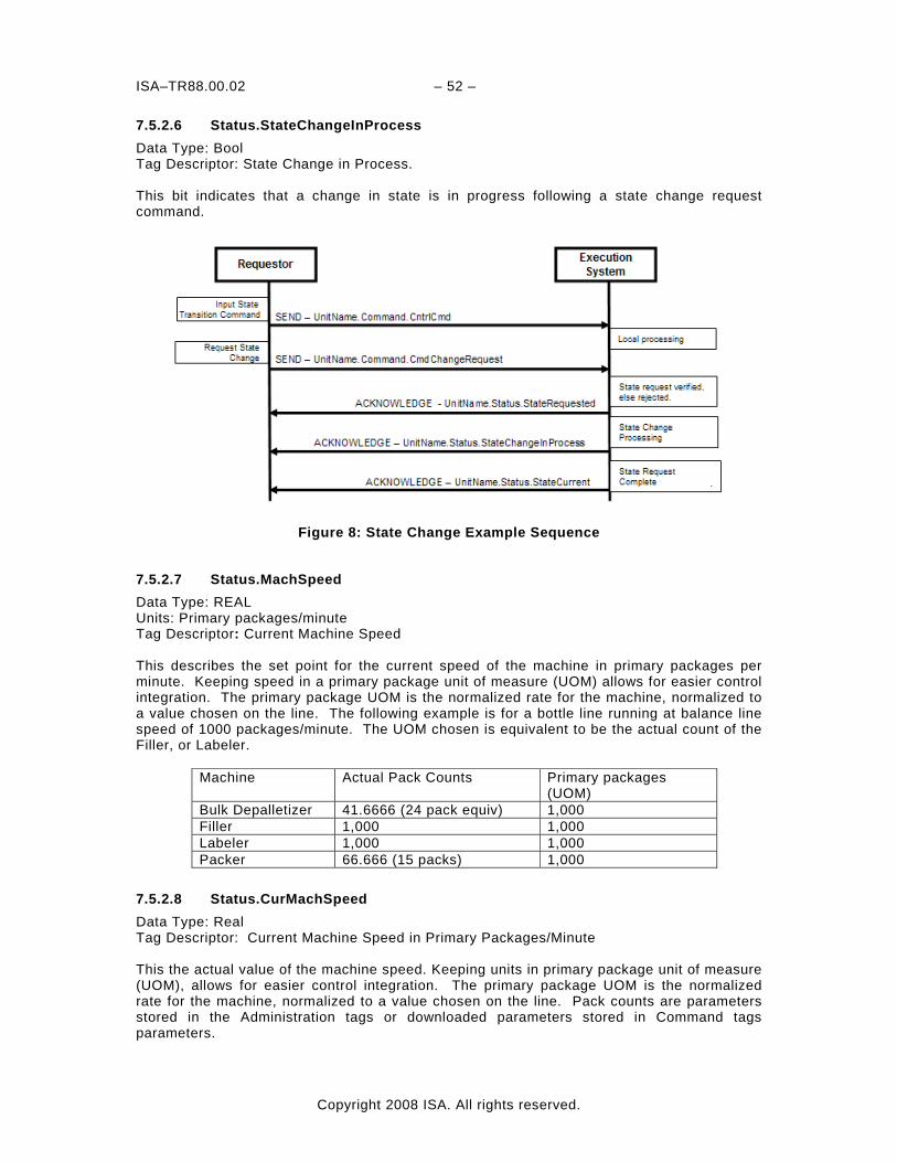
ISA–TR88.00.02 – 52 –


7.5.2.6 Status.StateChangeInProcess Data Type: Bool Tag Descriptor: State Change in Process. This bit indicates that a change in state is in progress following a state change request command.

Figure 8: State Change Example Sequence

7.5.2.7 Status.MachSpeed Data Type: REAL Units: Primary packages/minute Tag Descriptor: Current Machine Speed This describes the set point for the current speed of the machine in primary packages per minute. Keeping speed in a primary package unit of measure (UOM) allows for easier control integration. The primary package UOM is the normalized rate for the machine, normalized to a value chosen on the line. The following example is for a bottle line running at balance line speed of 1000 packages/minute. The UOM chosen is equivalent to be the actual count of the Filler, or Labeler.

Machine Actual Pack Counts Primary packages (UOM)

Bulk Depalletizer 41.6666 (24 pack equiv) 1,000 Filler 1,000 1,000 Labeler 1,000 1,000 Packer 66.666 (15 packs) 1,000

7.5.2.8 Status.CurMachSpeed Data Type: Real Tag Descriptor: Current Machine Speed in Primary Packages/Minute This the actual value of the machine speed. Keeping units in primary package unit of measure (UOM), allows for easier control integration. The primary package UOM is the normalized rate for the machine, normalized to a value chosen on the line. Pack counts are parameters stored in the Administration tags or downloaded parameters stored in Command tags parameters.

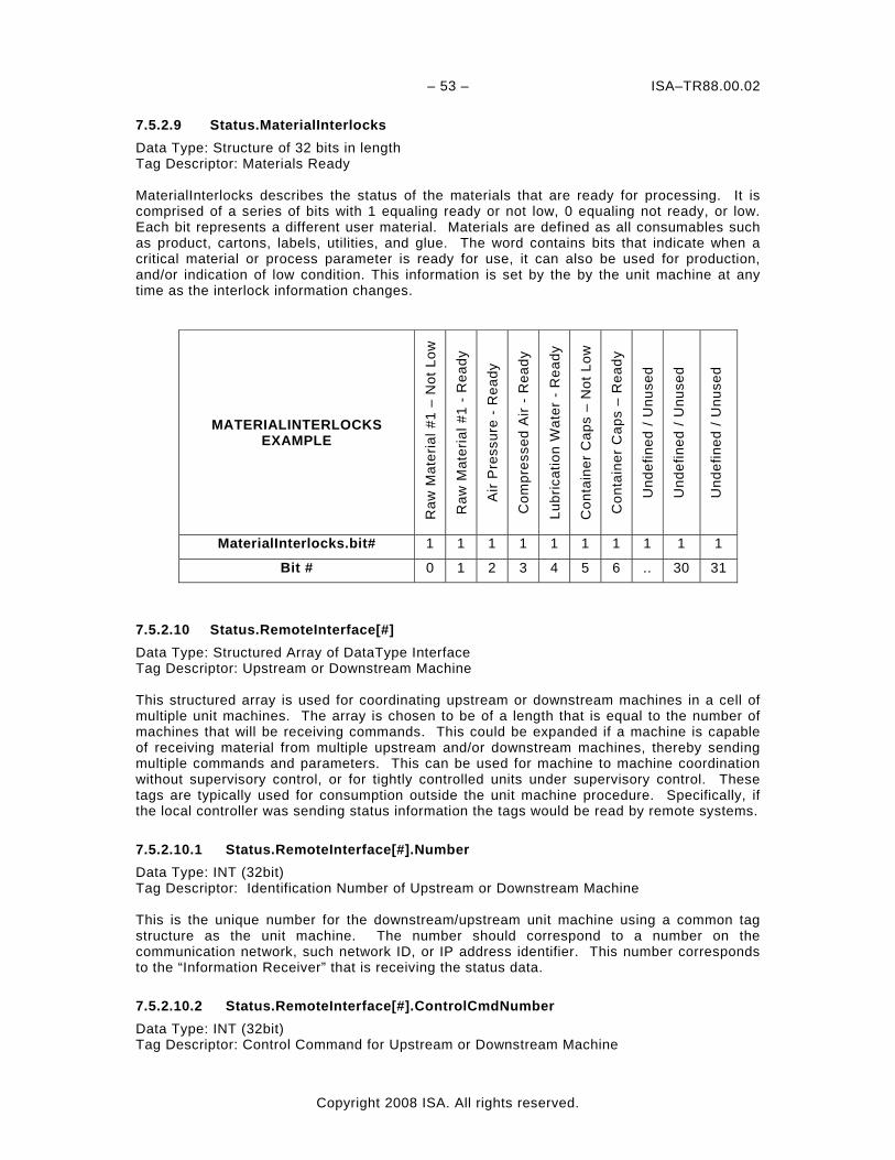
– 53 – ISA–TR88.00.02


7.5.2.9 Status.MaterialInterlocks Data Type: Structure of 32 bits in length Tag Descriptor: Materials Ready MaterialInterlocks describes the status of the materials that are ready for processing. It is comprised of a series of bits with 1 equaling ready or not low, 0 equaling not ready, or low. Each bit represents a different user material. Materials are defined as all consumables such as product, cartons, labels, utilities, and glue. The word contains bits that indicate when a critical material or process parameter is ready for use, it can also be used for production, and/or indication of low condition. This information is set by the by the unit machine at any time as the interlock information changes.

MATERIALINTERLOCKS EXAMPLE

Raw

Mat

eria

l #1

– N

ot L

ow

Raw

Mat

eria

l #1

- R

eady

Air

Pre

ssur

e -

Rea

dy

Com

pres

sed

Air

- R

eady

Lubr

icat

ion

Wat

er -

Rea

dy

Con

tain

er C

aps

– N

ot L

ow

Con

tain

er C

aps

– R

eady

Und

efin

ed /

Unu

sed

Und

efin

ed /

Unu

sed

Und

efin

ed /

Unu

sed

MaterialInterlocks.bit# 1 1 1 1 1 1 1 1 1 1

Bit # 0 1 2 3 4 5 6 .. 30 31

7.5.2.10 Status.RemoteInterface[#] Data Type: Structured Array of DataType Interface Tag Descriptor: Upstream or Downstream Machine This structured array is used for coordinating upstream or downstream machines in a cell of multiple unit machines. The array is chosen to be of a length that is equal to the number of machines that will be receiving commands. This could be expanded if a machine is capable of receiving material from multiple upstream and/or downstream machines, thereby sending multiple commands and parameters. This can be used for machine to machine coordination without supervisory control, or for tightly controlled units under supervisory control. These tags are typically used for consumption outside the unit machine procedure. Specifically, if the local controller was sending status information the tags would be read by remote systems. 7.5.2.10.1 Status.RemoteInterface[#].Number Data Type: INT (32bit) Tag Descriptor: Identification Number of Upstream or Downstream Machine This is the unique number for the downstream/upstream unit machine using a common tag structure as the unit machine. The number should correspond to a number on the communication network, such network ID, or IP address identifier. This number corresponds to the “Information Receiver” that is receiving the status data. 7.5.2.10.2 Status.RemoteInterface[#].ControlCmdNumber Data Type: INT (32bit) Tag Descriptor: Control Command for Upstream or Downstream Machine

ISA–TR88.00.02 – 54 –


A user defined command number associated with coded value to a remote unit. This number is a coded value sent from one node on the network to another. The value can be associated with a unit mode change request, speed change request, a state change request, etc. 7.5.2.10.3 Status.RemoteInterface[#].CmdValue Data Type: INT (32bit) Tag Descriptor: Control Command Value Associated ControlCmdNumber This is the status value associated with the ControlCmdNumber above. The status value may be the speed requested, state change, etc. EXAMPLE: For an upstream machine designated as #2 a control command number of 5 may be related to a speed setting value from machine #2. A value of 400 can be used to modify the current machine setpoint. Status.RemoteInterface[1].Number = 2 Status.RemoteInterface[1].ControlCmdNumber = 5 Status.RemoteInterface[1].CmdValue = 400 For a downstream machine designated as #4 the control command number of 0 can be used to read the command of a state transition from machine #4. The value of 2 is the command value for start. Status.RemoteInterface[1].Number = 4 Status.RemoteInterface[1].ControlCmdNumber = 0 Status.RemoteInterface[1].CmdValue = 2 7.5.2.10.4 Status.RemoteInterface[#].Parameter[#] Data Type: Structured Array of Data Type Descriptor The status Parameter tags are associated with the Remote Interface and are typically used for parameters that are sent to the remote machine(s) from the unit machine. The parameters are typically needed for coordinating the unit with other machines. The parameter value may be anything from machine limit parameters to temperatures and counter presets. The parameters are typically limited to machine parameters as product and process parameters are describe in later tags. 7.5.2.10.4.1 Status.RemoteInterface[#].Parameter[#].ID Data Type: INT (32bit) Tag Descriptor: ID Value of Parameter This is the arbitrary (user defined) ID value assigned to the parameter. This is non-descript value that can be used for user tag requirements. 7.5.2.10.4.2 Status.RemoteInterface[#].Parameter[#].Name Data Type: String Tag Descriptor: String Value Assigned to Parameter The literal parameter name is used to describe the parameter variable number, and its associated value from the unit machine. An example parameter name may be GLUE TEMP, BEARING TEMP, OVERLOAD TIME, etc. This is also could be displayed on HMI screens. 7.5.2.10.4.3 Status.RemoteInterface[#].Parameter[#].Unit Data Type: String[5] Tag Descriptor: String Value of Parameter Unit of Measure Unit is a string that describes the unit of measure associated with the parameter’s value (i.e., secs, deg, rpm, ppm, etc.). This tag describes the unit of measure associated with the following tag value that is sent from the unit machine.

– 55 – ISA–TR88.00.02


7.5.2.10.4.4 Status.RemoteInterface[#].Parameter[#].Value Data Type: REAL Tag Descriptor: Numeric Value of Parameter This is the numeric value of the parameter. The value is described by the Parameter[#].ID, Parameter[#].Name, and is of unit of measure that is parameterized by the Parameter[#].Unit. The value can be sent by the unit machine as information to a remote machine. 7.5.2.11 Status.Parameter[#] Data Type: Array of Data Type Descriptor The Parameter tags are associated with the local Interface and are typically used for parameters that are displayed or used on the unit locally, for example an HMI. These parameters can be a reflection of the command parameter tags or used to display any machine parameter. The parameters are typically needed for running the unit machine. The parameter value may be anything from machine limit parameters to temperatures and counter presets. The parameters are typically limited to machine parameters, as product and process parameters are described in later tags. The extent of the array is dependent on the number of parameters needed. 7.5.2.11.1 Status.Parameter[#].ID Data Type: INT (32bit) Tag Descriptor: ID Value of Parameter This is the arbitrary (user defined) ID value of the parameter. This is non-descript value that can be used for any user tag requirements. 7.5.2.11.2 Status.Parameter[#].Name Data Type: STRING Tag Descriptor: Structured Array of Parameter Variable Names for the Machine Unit The literal parameter name is used to describe the parameter number, and its associated value. An example parameter name may be GLUE TEMP, BEARING TEMP, OVERLOAD TIME, etc. This is also could be displayed on HMI screens. 7.5.2.11.3 Status.Parameter#].Unit Data Type: STRING[5] Tag Descriptor: Structured Array of Parameter Unit of Measure for the Machine Unit The parameter unit is used to describe the unit of measure of the parameter, and its associated value. An example parameter unit of measure may be DegF, secs, PPM, revs, mm, etc. This also could be displayed on HMI screens. 7.5.2.11.4 Status.Parameter[#].Value Data Type: Real Tag Descriptor: Structured Array of Parameter Values This is the numeric value of the parameter. The value is described by the Parameter[#].ID, Parameter[#].Name, and is a unit of measure described by the Parameter[#].Unit on the local machine. An example is the following: Status.Parameter[1].Value = 22.5 Status.Parameter[2].Value = 12 An example of a machine unit process variable:

ISA–TR88.00.02 – 56 –


Status.Parameter[1].Name = BEARING_1_OVERTEMP Status.Parameter[1].Unit = DegC Status.Parameter[1].Value = 350.00 This defines the temperature of a Bearing Overtemp alarm of the #1 bearing is to be set at 350.0 Degrees C for all products.

– 57 – ISA–TR88.00.02


7.5.2.12 Status.Product[#] Data Type: Array of Data Type Product The Product data type can be used for displaying product and product processing parameter variables. The status tags can come from either a local HMI or remote systems, and are used to display or send information on the product(s) on the unit machine. The array is typically needed for machines that run multiple products. 7.5.2.12.1 Status.Product[#].ProductID Data Type: INT (32bit) Tag Descriptor: Structured Array of Product ID# This Product ID is used to indicate to the machine which product it is producing (i.e., SKU or UPC). This can also be displayed on all HMI screens. The array can be used for machines that run multiple products. 7.5.2.12.2 Status.Product[#].ProcessVariables[#] Data Type: Array of Data Type Descriptor The ProcessVaribles structured array can be used to display specific process variables used by the unit machine for the processing of a specific product. Process variables include set points, limits, quality parameters, etc., that are displayed to produce a particular product on a unit machine. The number of tags for this array will be the maximum number of needed process variables for any particular product defined on the unit machine. 7.5.2.12.3 Status.Product[#].ProcessVariables[#].ID Data Type: INT (32bit) Tag Descriptor: ID Value of Parameter This is the arbitrary (user defined) process variable ID value assigned to the process variable. 7.5.2.12.4 Status.Product[#].ProcessVariables[#].Name Data Type: STRING Tag Descriptor: Structured Array of Process Variable Names for Multiple Product ID#s The process variable literal name is used to describe the process variable number, and its associated value. An example process variable name may be GLUE TEMP, MaxTimeInMachine, MixingTime, KnifeSpeed, ChillRollPhaseOffset, etc. This also could be displayed on HMI screens. 7.5.2.12.5 Status.Product[#].ProcessVariables[#].Unit Data Type: STRING[5] Tag Descriptor: Structured Array of Process Variable Unit of Measure for Multiple Product ID#s The process variable unit is used to describe the units of the process variable number, and its associated value. An example process unit name may be DegF, secs, PPM, revs, mm, etc. This also could be displayed on HMI screens. The array is typically needed for machines that run multiple products. 7.5.2.12.6 Status.Product[#].ProcessVariables[#].Value Data Type: Real Tag Descriptor: Structured array of Process Variable values

ISA–TR88.00.02 – 58 –


The process variable value is used to specify a process variable for the Product[#] specified by the ProcessVariable[#].ID, ProcessVariables[#].Name, and ProcessVariables[#].Unit. This also could be displayed on HMI screens. Status.Product[1].ProcessVariables[1].Value = 22.5 Status.Product[1].ProcessVariables[2].Value = 12 Combined with other examples of Product[#] Status.Product[1].ProcessVariables[1].Name = Glue1Temp Status.Product[1].ProcessVariables[1].Unit = DegF Status.Product[1].ProcessVariables[1].Value = 356.4 Meaning the temperature of at Glue station 1 is to be controlled at 356.4 Degrees F for product number 1. Other Examples of Process Variable Name For Products: Name = ProductMaxTimeInMachine Name = ProductMinTimeInMachine Name = ByproductID Name = ByproductsMaxTimeInMachine 7.5.2.12.7 Status.Product[#].Ingredients[#] Data Type: Array of Data Type Ingredient This array serves to hold the information needed for the raw materials that are used by the unit machine in the processing of a particular product. The extent of this array will be the maximum number of ingredients used in the processing of any particular product. 7.5.2.12.7.1 Status.Product[#].Ingredients[#].IngredientID Data Type: INT (32bit) Tag Descriptor: Structured Array of Ingredient IDs The IngredientID is an arbitrary number associated with the raw material, or ingredient for a particular product number. The user will define the value associated to the ingredient IDs that are used in the operation of the machine for a particular product. Each ingredient should have a distinct ID (SKU or UPC). 7.5.2.12.7.2 Status.Product[#].Ingredients[#].Parameter[#] Data Type: Array of Data Type Descriptor This array of structures is used for parameters associated with a particular ingredient or raw material used the processing of a particular product number. This status tag is typically set by the unit machine controller. The extent of this array is the maximum number of parameters associated with any ingredient in any product that is defined on the unit machine. 7.5.2.12.7.2.1 Status.Product[#].Ingredients[#].Parameter[#].ID Data Type: INT (32bit) Tag Descriptor: ID Value of Parameter This is the arbitrary (user defined) ID value assigned to one of the parameters for the ingredient or raw material, needed for the processing of the product defined by the product number. 7.5.2.12.7.2.2 Status.Product[#].Ingredients[#].Parameter[#].Name Data Type: STRING

– 59 – ISA–TR88.00.02


Tag Descriptor: Structured Array of Ingredient Parameter Names The parameter variable name in the parameter array is used to describe the parameter names associated with a specific ingredient number in a specific product number. An example parameter name may be SETUP TIME, TEMP, TAB POSITION, etc. This also could be displayed on HMI screens. The array is typically needed for machines that run multiple ingredients with multiple parameters with multiple products. 7.5.2.12.7.2.3 Status.Product[#].Ingredients[#].Parameter[#].Unit Data Type: STRING[5] Tag Descriptor: Structured Array of Unit of Measure The parameter unit tag is used to describe the parameter names associated with a specific parameter in a specific ingredient in a specific product. An example process unit of measure name may be DegF, secs, PPM, revs, mm, etc. This also could be displayed on HMI screens. The array is typically needed for unit machines that run multiple products with multiple ingredients with multiple processing parameters. 7.5.2.12.7.2.4 Status.Product[#].Ingredients[#].Parameter[#].Value Data Type: Real Tag Descriptor: Structured array of values The ingredient parameter value is used to specify a parameter variable for displaying information about the process. This also could be displayed on HMI screens. The array is typically needed for unit machines that run multiple products with multiple ingredients with multiple processing parameters. As an example with Ingredient number 1 in Product number 1: Status.Product[1].Ingredients[1].Parameter[1].Value = 225 Status.Product[1].Ingredients[1].Parameter[2].Value = 12 Combined with other examples of Product[#] Status.Product[1].Ingredients[1].Parameter[1].Name = KNIFE_OFFSET Status.Product[1].Ingredients[1].Parameter[1].Unit = degrees Status.Product[1].Ingredients[1].Parameter[1].Value = 3.564 Meaning the offset of the knife is to be controlled at 3.564 Degrees for Parameter variable number 1, on ingredient 1 for product number 1.

ISA–TR88.00.02 – 60 –


7.5.3 Administration Tags Administration tags are used to describe the quality and alarm information of the unit machine. Administration tags include alarm parameters which describe the conditions within the Base State model typically for production data acquisition (PDA) systems. The administration tags also include parameters which can describe how well the machine operates, or specifically information on the product quality produced by the machine. Administration tags generally originate from the unit machine and can be used on the HMI or a remote system. 7.5.3.1 Admin.Parameter[#] Data Type: Array of Data Type Descriptor The Parameter tags associated to the local interface are typically used for as parameters that are displayed or used on the unit locally, for example from an HMI. These parameters can be used to display any quality, alarm, or machine downtime parameter. The parameters are typically limited to parameters related the unit. The extent of the array is the maximum number of parameters needed. 7.5.3.1.1 Admin.Parameter[#].ID Data Type: INT (32bit) Tag Descriptor: ID Value of Parameter This is the arbitrary (user defined) ID value of the parameter. This is non-descript value that can be used for any user tag requirements 7.5.3.1.2 Admin.Parameter[#].Name Data Type: STRING Tag Descriptor: Structured Array of Parameter Names for the Machine Unit The parameter name is used to describe the parameter number, and its associated value. An example parameter name may be CASES MADE, OPERATOR SHIFT, REJECTED PRODUCTS, etc. This also could be displayed on HMI screens. The array is typically needed for machines that have quality reporting or PDA (Production Data Acquisition) needs. 7.5.3.1.3 Admin.Parameter[#].Unit Data Type: STRING[5] Tag Descriptor: Structured Array of Parameter Variable Unit of Measure for the Machine Unit The administration parameter unit of measure is used to describe the unit of measure of the parameter, and its associated value. An example parameter unit of measure may be CASES, PROD, PPM, etc. This also could be displayed on HMI screens. 7.5.3.1.4 Admin.Parameter[#].Value Data Type: Real Tag Descriptor: Structured Array of Parameter Values The parameter value is used to specify a unit machine variable for use in the PDA or to be sent to an “information receiver”. This is also could be displayed on HMI screens. As an example: Admin.Parameter[1].Value = 50019 An example of a machine unit process variable: Admin.Parameter[1].Name = TOTAL PRODUCTION Admin.Parameter[1].Unit = STAT

– 61 – ISA–TR88.00.02


Admin.Parameter[1].Value = 50010. 7.5.3.2 Admin.Alarm[#] Data Type: Alarm Descriptor: Array of Given Size for Machine Fault Number and Messaging The Alarm tags associated with the local interface are typically used as parameters that are displayed or used on the unit locally, for example from a HMI. These alarm parameters can be used to display any alarm, or machine downtime cause that is currently occurring in the system. The alarms are typically limited to the machine unit. The extent of the array is the maximum number of alarms needed to be annunciated. 7.5.3.2.1 Admin.Alarm[#].ID Data Type: INT (32bit) Tag Descriptor: Alarm Message Identification Number The Alarm ID number is an unique value assigned to each alarm. The ID can be used for any general alarms and faults (alarms detailed in Appendix A). 7.5.3.2.2 Admin.Alarm[#].Value Data Type: INT (32bit) Tag Descriptor: Alarm Message Number The Alarm Message number is a value that is associated with the alarm allowing for user specific detail, or to break down the Alarm.ID to greater detail (alarms detailed in Appendix A). For instance an Alarm[#].ID value of 4 from Appendix A may require a more detailed breakdown as shown in Appendix A. 7.5.3.2.3 Admin.Alarm[#].Message Data Type: String Tag Descriptor: Alarm Message The alarm message is the actual text of the alarm for those machines capable of reading the string information. 7.5.3.2.4 Admin.Alarm[#].TimeEvent Data Type: TimeStamp Structure of date and time in the alarm array to detail the date and time the alarm occurred. 7.5.3.2.4.1 Admin.Alarm[#].TimeEvent.AlmDate Data Type: Date Tag Descriptor: ISO Date Data type Defines the date the alarm has occurred in ISO 8601:1988 format (defines as seconds from January 1, 1970 at 12:00am). 7.5.3.2.4.2 Admin.Alarm[#].TimeEvent.AlmTime Data Type: Time Tag Descriptor: ISO Time Data Type Defines the time the alarm has occurred in ISO 8601:1988 format (defines as seconds from January 1, 1970 at 12:00am).

ISA–TR88.00.02 – 62 –


7.5.3.2.5 Admin.Alarm[#].TimeAck Data Type: TimeStamp Structure of date and time in the alarm array to detail the date and time the alarm was acknowledged. 7.5.3.2.5.1 Admin.Alarm[#].TimeAck.AlmDate Data Type: Date Tag Descriptor: ISO Date Data type Defines the time the alarm was acknowledged in ISO 8601:1988 format (defines as seconds from January 1, 1970 at 12:00am). 7.5.3.2.5.2 Admin.Alarm[#].TimeAck.AlmTime Data Type: Time Tag Descriptor: ISO Time Data Type Defines the date the alarm was acknowledged in ISO 8601:1988 format (defines as seconds from January 1, 1970 at 12:00am). The following is an example of how the Alarm structure may appear: The alarm array is for currently occurring alarms and will can be sorted in chronological order with the most recently occurring alarmed indexed as Admin.Alarm[0]. Any unused elements in the array should be set to the following values:

Admin.Alarm[#].ID 0 Admin.Alarm[#].Value 0 Admin.Alarm[#].Message “” Admin.Alarm[#].TimeEvent.AlmDate 0 Admin.Alarm[#].TimeEvent.AlmTime 0 Admin.Alarm[#].TimeAck.AlmDate 0 Admin.Alarm[#].TimeAck.AlmTime 0

7.5.3.3 Admin.AlarmExtent Data Type: INT (32bit) Tag Descriptor: Extent of Alarm Array The alarm extent is associated with the maximum number of alarms needed for the machine annunciation or reporting. This tag can be used by a remote machine to understand the extent of the alarm array, or locally to manage the use of the array.

7.5.3.4 Admin.AlarmHistory[#] Data Type: Alarm Descriptor: Array of Given Size for Machine Fault Number and Messaging History The Alarm tags associated to the local interface are typically used for parameters that are displayed or used on the unit locally, for example for a HMI. These alarm history parameters can be used to display any alarm history, or machine downtime cause. The historical alarms are typically limited to the machine unit. The extent of the array is the maximum number of historical alarms needed. 7.5.3.4.1 Admin.AlarmHistory[#].ID Data Type: INT (32bit) Tag Descriptor: Alarm Message Identification Number

– 63 – ISA–TR88.00.02


The Alarm ID number is an unique value assigned to each alarm. The ID can be used for any general alarms and faults (alarms detailed in Appendix A). 7.5.3.4.2 Admin.AlarmHistory[#].Value Data Type: INT (32bit) Tag Descriptor: Alarm Message Number The Alarm Message number is a value that is associated with the alarm allowing for user specific detail, or to break down the Alarm.ID to greater detail (alarms detailed in Appendix A). For instance an Alarm[#].ID value of 4 from Appendix A may require a more detailed breakdown as shown in Appendix A. 7.5.3.4.3 Admin.AlarmHistory[#].Message Data Type: String Tag Descriptor: Alarm Message The alarm message is the actual text of the alarm for those machines capable of reading the string information. 7.5.3.4.4 Admin.AlarmHistory[#].TimeEvent Data Type: TimeStamp Structure of date and time in the alarm array to detail the date and time the alarm occurred. 7.5.3.4.4.1 Admin.AlarmHistory[#].TimeEvent.AlmDate Data Type: Date Tag Descriptor: ISO Date Data Type Defines the date the alarm has occurred in ISO 8601:1988 format (defines as seconds from January 1, 1970 at 12:00am). 7.5.3.4.4.2 Admin.AlarmHistory[#].TimeEvent.AlmTime Data Type: Date Tag Descriptor: ISO Time Data Type Defines the Time the alarm has occurred in ISO 8601:1988 format (defines as seconds from January 1, 1970 at 12:00am). 7.5.3.4.5 Admin.AlarmHistory[#].TimeAck Data Type: TimeStamp Structure of date and time in the alarm array to detail the date and time the alarm was acknowledged. 7.5.3.4.5.1 Admin.AlarmHistory[#].TimeAck.AlmDate Data Type: Date Tag Descriptor: ISO Date Data Type Defines the date the alarm has occurred in ISO 8601:1988 format (defines as seconds from January 1, 1970 at 12:00am). 7.5.3.4.5.2 Admin.AlarmHistory[#].TimeAck.AlmTime Data Type: Date Tag Descriptor: ISO Time Data Type

ISA–TR88.00.02 – 64 –


Defines the Time the alarm has occurred in ISO 8601:1988 format (defines as seconds from January 1, 1970 at 12:00am). The following is an example of how the AlarmHistory structure may appear: The AlarmHistory array is reserved for alarms that have occurred and can be sorted in chronological order with the most recently occurring alarmed indexed as Admin.AlarmHistory[0].

Any unused elements should be set to the following values

Admin.AlarmHistory[#].ID 0 Admin.AlarmHistory[#].Value 0 Admin.AlarmHistory[#].Message “” Admin.AlarmHistory[#].TimeEvent.AlmDate 0 Admin.AlarmHistory[#].TimeEvent.AlmTime 0 Admin.AlarmHistory[#].TimeAck.AlmDate 0 Admin.AlarmHistory[#].TimeAck.AlmTime 0

7.5.3.5 Admin.AlarmHistoryExtent Data Type: INT (32bit) Tag Descriptor: Extent of Alarm History Array The alarm history extent is associated with the maximum number of alarms needed to be archived or tagged as alarm history for the machine. This tag can be used by a remote machine to understand the extent of the alarm array, or locally to manage the array.

7.5.3.6 Admin.ModeCurrentTime[#] Data Type: INT (32bit) Unit of Measure: sec Tag Descriptor: Array of Timer Values This tag represents the current amount of time (in sec) in any defined unit mode. The array index is equal to the designation of the of the unit machine mode values – defined in Status.UnitModeCurrent. The values roll over to 0 at 2,147,483,647. 7.5.3.7 Admin.ModeCumulativeTime[#] Data Type: INT (32bit) Unit of Measure: sec Tag Descriptor: Array of Timer Values This tag represents the cumulative amount of time (in sec) in any defined unit mode. The array index is equal to the designation of the of the unit machine mode values – defined in Status.UnitModeCurrent. The value is the cumulative elapsed time the machine has spent in each mode since its timers and counters were reset. The values roll over to 0 at 2,147,483,647. 7.5.3.8 Admin.StateCurrentTime[#,#] Data Type: INT (32bit) Unit of Measure: sec Tag Descriptor: Array of Timer Values This tag represents the current amount of time (in sec) in any defined state in any particular mode. The array index is equal to the designation of the of the unit machine mode values defined in Status.UnitModeCurrent, and the state values defined in Status.StateCurrent; such that the array index is [Status.UnitModeCurrent, Status.StateCurrent]. The values roll over to 0 at 2,147,483,647.

– 65 – ISA–TR88.00.02


7.5.3.9 Admin.StateCumulativeTime[#,#] Data Type: INT (32bit) Unit of Measure: sec Tag Descriptor: Array of Timer Values This tag represents the cumulative amount of time (in sec) in any defined state in any particular mode since the last timer and counter reset was executed. The array index is equal to the designation of the of the unit machine mode values defined in Status.UnitModeCurrent, and the state values defined in Status.StateCurrent; such that the array index is [Status.UnitModeCurrent, Status.StateCurrent]. The values roll over to 0 at 2,147,483,647. 7.5.3.10 Admin.ProdConsumedCount[#] Data Type: Array of Data Type ProdCount This tag represents the material used/consumed in the production machine. An example of tag usage would be the number of bags consumed in a Filler, or bagger packaging machine, or the amount of linear length used, or the number caps used. This tag can be used locally or remotely if needed. The extent of the array is typically limited to the number of raw materials needed to be counted. The array is typically used for unit machines that run multiple raw materials. This array may also be used to track the number of unfinished products entering a machine for processing, but typically Admin.ProdProcessedCount[#] is used for this. 7.5.3.10.1 Admin.ProdConsumedCount[#].ID Data Type: INT (32bit) Tag Descriptor: ID Value of ProdConsumedCount This is the arbitrary (user defined) ID value of the consumed production material. This is non-descript value that can be used for any user tag requirements. The ID value can be SKU or a user specific material identifier. 7.5.3.10.2 Admin.ProdConsumedCount[#].Name Data Type: STRING Tag Descriptor: Structured Array of Names in ProdConsumedCount The name is used to literally describe the material ID, and its associated material. An example parameter name may be PRODUCT A BAGS, XYZ CAPS FOR ABC PRODUCT, etc. This also could be displayed on HMI screens. The array is typically needed for machines that have quality reporting or PDA (Production Data Acquisition) needs. 7.5.3.10.3 Admin.ProdConsumedCount[#].Unit Data Type: STRING[5] Tag Descriptor: Structured Array of Units in ProdConsumedCount The unit tag is used to describe the names associated with a specific material used by the machine. An example process unit of measure name may be FT, CNT, KG, etc. This also could be displayed on HMI screens. 7.5.3.10.4 Admin.ProdConsumedCount[#].Count Data Type: Int(32bit) Tag Descriptor: Structured Array of Values The count value is used as a variable for displaying information about the amount of consumed production material. The value is indexed upon the machine consuming a unit of the material defined by the ID and NAME. This could be displayed on HMI screens or higher level PDA systems. The counter rolls over to 0 at 2,147,483,648.

ISA–TR88.00.02 – 66 –


7.5.3.10.5 Admin.ProdConsumedCount[#].AccCount Data Type: Int(32bit) Tag Descriptor: Structured Array of Values The accumulative count value is used as a variable for displaying information about the total amount of consumed production material. The value is indexed upon the machine consuming a unit of the material defined by the ID and NAME. This could be displayed on HMI screens or higher level PDA systems. This counter gives the user a non-resetting counter that may be used for OEE calculations. The counter rolls over to 0 at 2,147,483,648. An example of the Production Consumption counter is the following: Admin.ProdConsumedCount[1].ID = 546732 Admin.ProdConsumedCount[1].Name = LABELS FOR XYZ Admin.ProdConsumedCount[1].Units = CNT Admin.ProdConsumedCount[1].Count = 2305 Admin.ProdConsumedCount[1].AccCount = 14,995,100 The above describes consumed labels used by the machine for product XYZ as being 2305 since the last operator reset and 14,995,100 since the last accumulative counter reset. 7.5.3.11 Admin.ProdProcessedCount[#] Data Type: Array of Data Type ProdCount This tag represents the number of products processed by the production machine. An example of tag usage would be the number of products that were made, including all good and defective products. This tag can be used locally or remotely if needed. The extent of the array is typically limited to the number of products needed to be counted. The number of products processed minus the defective count is the number of products made by the machine. The array index of # = 0 can be reserved for the count of the number of units from the primary production stream. 7.5.3.11.1 Admin.ProdProcessedCount[#].ID Data Type: INT (32bit) Tag Descriptor: ID Value of ProdProcessedCount This is the arbitrary (user defined) ID value of the processed products. This is non-descript value that can be used for any user tag requirements. The ID value can be SKU or a user specific product identifier. 7.5.3.11.2 Admin.ProdProcessedCount[#].Name Data Type: STRING Tag Descriptor: Structured Array of Names in ProdProcessedCount The name is used to literally describe the product ID. An example parameter name may be PRODUCT A, ABC PRODUCT, etc. This also could be displayed on HMI screens. The array is typically needed for machines that have quality reporting or PDA (Production Data Acquisition) needs. 7.5.3.11.3 Admin.ProdProcessedCount[#].Unit Data Type: STRING[5] Tag Descriptor: Structured Array of Units in ProdProcessedCount The unit tag is used to describe the names associated with a specific product used by the machine. An example process unit of measure name may be FT, CNT, KG, etc. This also could be displayed on HMI screens.

– 67 – ISA–TR88.00.02


7.5.3.11.4 Admin.ProdProcessedCount[#].Count Data Type: Int(32bit) Tag Descriptor: Structured Array of Values The count value is used as a variable for displaying information about the amount of processed product. The value is indexed upon the machine processing a unit of the product defined by the ID and NAME. This could be displayed on HMI screens or higher level PDA systems. The counter rolls over to 0 at 2,147,483,648. 7.5.3.11.5 Admin.ProdProcessedCount[#].AccCount Data Type: Int(32bit) Tag Descriptor: Structured Array of Values The accumulative count value is used as a variable for displaying information about the amount of processed product. The value is indexed upon the machine processing a unit of the product defined by the ID and NAME. This could be displayed on HMI screens or higher level PDA systems. This counter gives the user a non-resetting counter that may be used for OEE calculations. The counter rolls over to 0 at 2,147,483,648. An example of the production processed counter is the following: Admin.ProdProcessedCount[1].ID = 546732 Admin.ProdProcessedCount[1].Name = XYZ Product Admin.ProdProcessedCount[1].Units = CNT Admin.ProdProcessedCount[1].Count = 2305 Admin.ProdProcessedCount[1].AccCount = 2305 This describes the number of processed products the machine has made for product XYZ, i.e., 2305 products were processed by the machine. 7.5.3.12 Admin.ProdDefectiveCount[#] Data Type: Array of Data Type ProdCount This tag represents the product that is marked as defective in the production machine, to be used if applicable. An example of tag usage would be the number of products rejected or products that are termed defective. This tag can be used locally or remotely if needed. The extent of the array is typically limited to the number of products needed to be counted as defective. When this tag is used with Admin.ProdProcessedCount[#], the number of good products/well formed cycles made by the machine can be calculated. The array index of # = 0 can be reserved for the total cumulative rejected units from the primary production stream. 7.5.3.12.1 Admin.ProdDefectiveCount[#].ID Data Type: INT (32bit) Tag Descriptor: ID Value of ProdDefectiveCount This is the arbitrary (user defined) ID value of the defective production material. This is non-descript value that can be used for any user tag requirements. The ID value can be SKU or a user specific material identifier. 7.5.3.12.2 Admin.ProdDefectiveCount[#].Name Data Type: STRING Tag Descriptor: Structured Array of Names in ProdDefectiveCount The name is used to literally describe the product ID, and its associated material. An example parameter name may be PRODUCT A, XYZ PRODUCT, etc. This also could be displayed on

ISA–TR88.00.02 – 68 –


HMI screens. The array is typically needed for machines that have quality reporting or PDA (Production Data Acquisition) needs. 7.5.3.12.3 Admin.ProdDefectiveCount[#].Unit Data Type: STRING[5] Tag Descriptor: Structured Array of Units in ProdDefectiveCount The unit tag is used to describe the names associated with a specific product processed by the machine. An example process unit of measure name may be FT, CNT, KG, etc. This also could be displayed on HMI screens. The array is typically used for unit machines that run multiple products. 7.5.3.12.4 Admin.ProdDefectiveCount[#].Count Data Type: Int(32bit) Tag Descriptor: Structured Array of Values The count value is used as a variable for displaying information about the amount of defective product. The value is indexed upon the machine using a unit of the material defined by the ID and NAME. This could be displayed on HMI screens or higher level PDA systems. The counter rolls over to 0 at 2,147,483,648. 7.5.3.12.5 Admin.ProdDefectiveCount[#].AccCount Data Type: Int(32bit) Tag Descriptor: Structured Array of Values The accumulative count value is used as a variable for displaying information about the amount of defective product. The value is indexed upon the machine using a unit of the material defined by the ID and NAME. This could be displayed on HMI screens or higher level PDA systems. This counter gives the user a non-resetting counter that may be used for OEE calculations. The counter rolls over to 0 at 2,147,483,648. An example of the production defective counter is the following: Admin.ProdDefectiveCount[1].ID = 546732 Admin.ProdDefectiveCount[1].Name = XYZ Product Admin.ProdDefectiveCount[1].Units = CNT Admin.ProdDefectiveCount[1].Count = 1005 Admin.ProdDefectiveCount[1].AccCount = 3001 This describes defective products made by the machine (i.e., 1005 defective products made since the last reset of count and 3001 defective products since the last reset of AccCount). 7.5.3.13 Admin.AccTimeSinceReset Data Type: Int(32bit) Unit of Measure: Secs Tag Descriptor: Accumulative Time Since Last Reset The tag represents the amount of time since the reset has been triggered. When a reset is triggered all resettable tags are reset which can include: UnitName.Admin.ModeCurrentTime[#] UnitName.Admin.ModeCumulativeTime[#] UnitName.Admin.StateCurrentTime[#,#] UnitName.Admin.StateCumulativeTime[#,#] UnitName.Admin.ProdConsumedCount[#].Count UnitName.Admin.ProdProcessedCount[#].Count UnitName.Admin.ProdDefectiveCount[#].Count UnitName.Admin.AccTimeSinceReset.

– 69 – ISA–TR88.00.02


This value rolls over at 2,147,483,648 to 0. The tag can be used for simple OEE calculations as the definition of “scheduled production time”. The simple OEE calculation is the total amount of good products divided by the total amount of good products that can be produced with the unit time, with the unit of time being scheduled production time. 7.5.3.14 Admin.MachDesignSpeed Data Type: Real Unit of Measure: Primary Packages/minute Tag Descriptor: Machine Design Speed This tag represents the maximum design speed of the machine in primary packages per minute for the package configuration being run. This speed is NOT the maximum speed as specified by the manufacturer, but rather the speed the machine is designed to run in its installed environment. NOTE: In practice the maximum speed of the machine as used for efficiency calculations will be a function of how it is set up and what products it is producing. 7.5.3.15 Admin.PACDateTime Data Type: TimeStamp This tag defines the structure of date and time of the Programmable Automation Controller (PAC). The tag can be used to synchronize the clock with the PAC to the higher level systems used for OEE calculations. 7.5.3.15.1 Admin.PACDateTime.Date Data Type: Date Tag Descriptor: ISO Date Data Type Defines the date within the PAC in ISO 8601:1988 format (defines as seconds from January 1, 1970 at 12:00am). 7.5.3.15.2 Admin.PACDateTime.Time Data Type: Time Tag Descriptor: ISO Time Data Type Defines the time within the PAC in ISO 8601:1988 format (defines as seconds from January 1, 1970 at 12:00am).

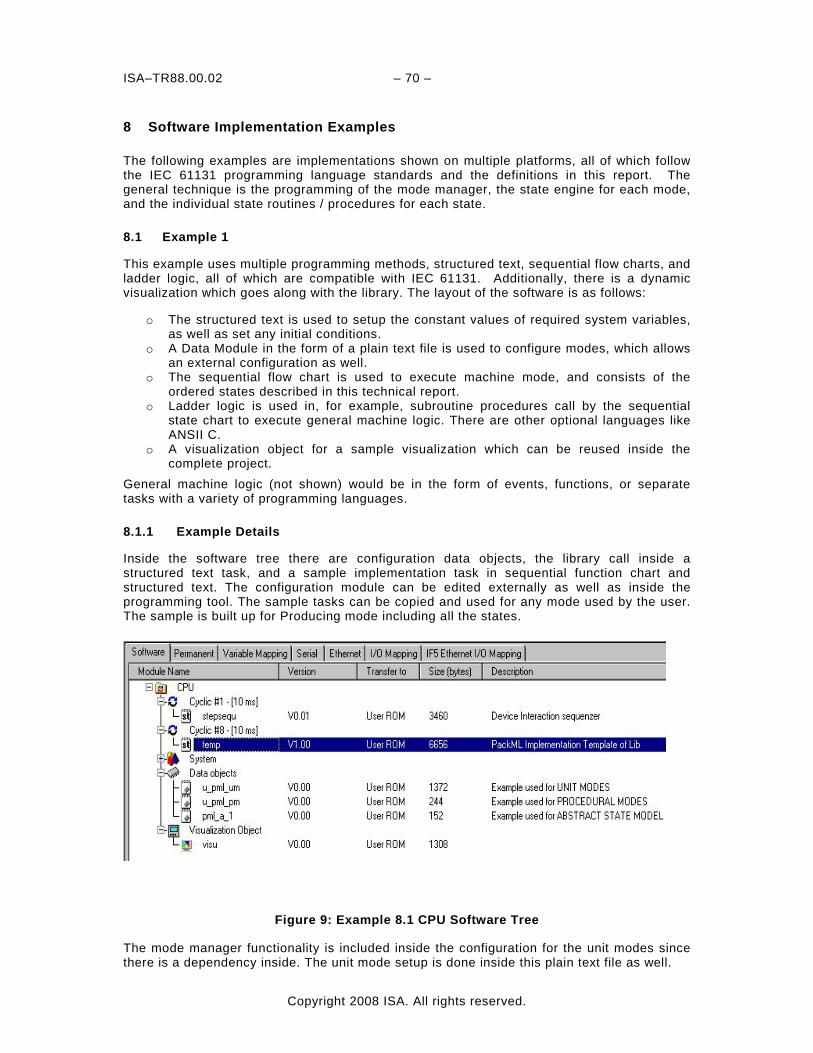
ISA–TR88.00.02 – 70 –


8 Software Implementation Examples

The following examples are implementations shown on multiple platforms, all of which follow the IEC 61131 programming language standards and the definitions in this report. The general technique is the programming of the mode manager, the state engine for each mode, and the individual state routines / procedures for each state.

8.1 Example 1

This example uses multiple programming methods, structured text, sequential flow charts, and ladder logic, all of which are compatible with IEC 61131. Additionally, there is a dynamic visualization which goes along with the library. The layout of the software is as follows:

o The structured text is used to setup the constant values of required system variables, as well as set any initial conditions.

o A Data Module in the form of a plain text file is used to configure modes, which allows an external configuration as well.

o The sequential flow chart is used to execute machine mode, and consists of the ordered states described in this technical report.

o Ladder logic is used in, for example, subroutine procedures call by the sequential state chart to execute general machine logic. There are other optional languages like ANSII C.

o A visualization object for a sample visualization which can be reused inside the complete project.

General machine logic (not shown) would be in the form of events, functions, or separate tasks with a variety of programming languages.

8.1.1 Example Details

Inside the software tree there are configuration data objects, the library call inside a structured text task, and a sample implementation task in sequential function chart and structured text. The configuration module can be edited externally as well as inside the programming tool. The sample tasks can be copied and used for any mode used by the user. The sample is built up for Producing mode including all the states.

Figure 9: Example 8.1 CPU Software Tree

The mode manager functionality is included inside the configuration for the unit modes since there is a dependency inside. The unit mode setup is done inside this plain text file as well.

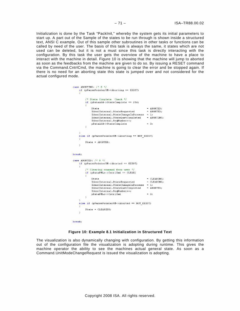
– 71 – ISA–TR88.00.02


Initialization is done by the Task “PackInit,” whereby the system gets its initial parameters to start up. A part out of the Sample of the states to be run through is shown inside a structured text, ANSI C example. Out of this sample other subroutines in other tasks or functions can be called by need of the user. The basis of this task is always the same, it states which are not used can be deleted, but it is not a must since this task is directly interacting with the configuration. By this task the user gets the overview of the machine to have a place to interact with the machine in detail. Figure 10 is showing that the machine will jump to aborted as soon as the feedbacks from the machine are given to do so. By issuing a RESET command via the Command.CntrlCmd, the machine is going to clear the error and be stopped again. If there is no need for an aborting state this state is jumped over and not considered for the actual configured mode.

Figure 10: Example 8.1 Initialization in Structured Text

The visualization is also dynamically changing with configuration. By getting this information out of the configuration file the visualization is adopting during runtime. This gives the machine operator the ability to see the machines actual general state. As soon as a Command.UnitModeChangeRequest is issued the visualization is adopting.

ISA–TR88.00.02 – 72 –


Figure 11: Example 8.1 Visualization Sample of Operator Interface

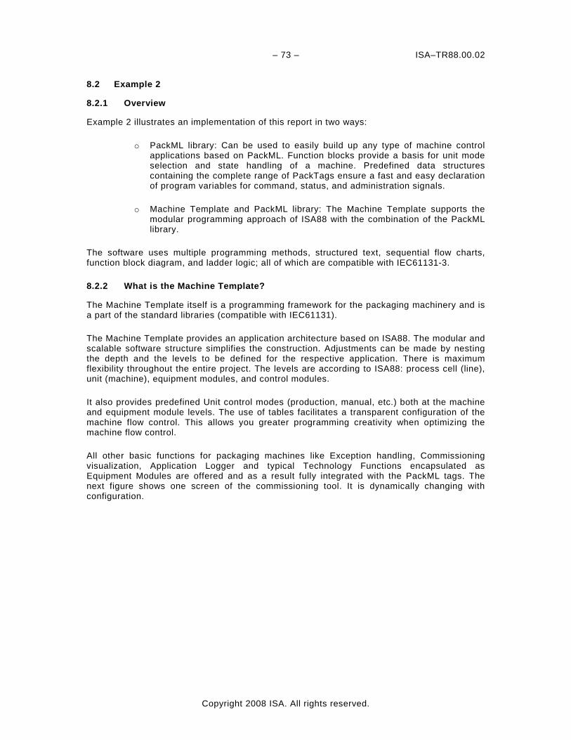
– 73 – ISA–TR88.00.02


8.2 Example 2

8.2.1 Overview

Example 2 illustrates an implementation of this report in two ways:

o PackML library: Can be used to easily build up any type of machine control applications based on PackML. Function blocks provide a basis for unit mode selection and state handling of a machine. Predefined data structures containing the complete range of PackTags ensure a fast and easy declaration of program variables for command, status, and administration signals.

o Machine Template and PackML library: The Machine Template supports the modular programming approach of ISA88 with the combination of the PackML library.

The software uses multiple programming methods, structured text, sequential flow charts, function block diagram, and ladder logic; all of which are compatible with IEC61131-3.

8.2.2 What is the Machine Template?

The Machine Template itself is a programming framework for the packaging machinery and is a part of the standard libraries (compatible with IEC61131).

The Machine Template provides an application architecture based on ISA88. The modular and scalable software structure simplifies the construction. Adjustments can be made by nesting the depth and the levels to be defined for the respective application. There is maximum flexibility throughout the entire project. The levels are according to ISA88: process cell (line), unit (machine), equipment modules, and control modules.

It also provides predefined Unit control modes (production, manual, etc.) both at the machine and equipment module levels. The use of tables facilitates a transparent configuration of the machine flow control. This allows you greater programming creativity when optimizing the machine flow control.

All other basic functions for packaging machines like Exception handling, Commissioning visualization, Application Logger and typical Technology Functions encapsulated as Equipment Modules are offered and as a result fully integrated with the PackML tags. The next figure shows one screen of the commissioning tool. It is dynamically changing with configuration.

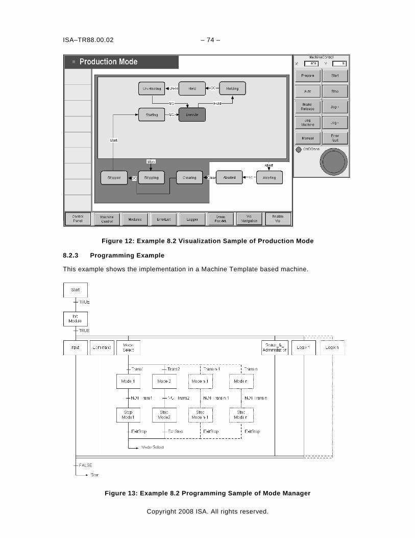
ISA–TR88.00.02 – 74 –


Figure 12: Example 8.2 Visualization Sample of Production Mode

8.2.3 Programming Example

This example shows the implementation in a Machine Template based machine.

Figure 13: Example 8.2 Programming Sample of Mode Manager

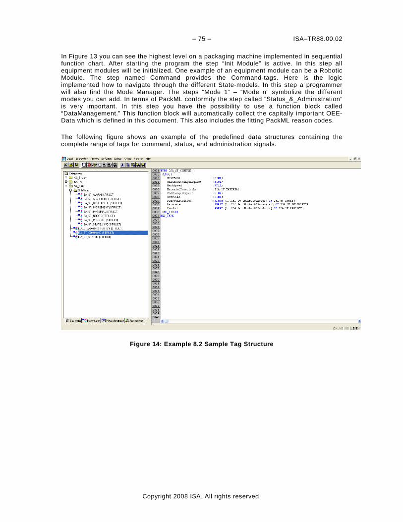
– 75 – ISA–TR88.00.02


In Figure 13 you can see the highest level on a packaging machine implemented in sequential function chart. After starting the program the step “Init Module” is active. In this step all equipment modules will be initialized. One example of an equipment module can be a Robotic Module. The step named Command provides the Command-tags. Here is the logic implemented how to navigate through the different State-models. In this step a programmer will also find the Mode Manager. The steps “Mode 1” – “Mode n” symbolize the different modes you can add. In terms of PackML conformity the step called ”Status_&_Administration“ is very important. In this step you have the possibility to use a function block called “DataManagement.” This function block will automatically collect the capitally important OEE-Data which is defined in this document. This also includes the fitting PackML reason codes.

The following figure shows an example of the predefined data structures containing the complete range of tags for command, status, and administration signals.

Figure 14: Example 8.2 Sample Tag Structure

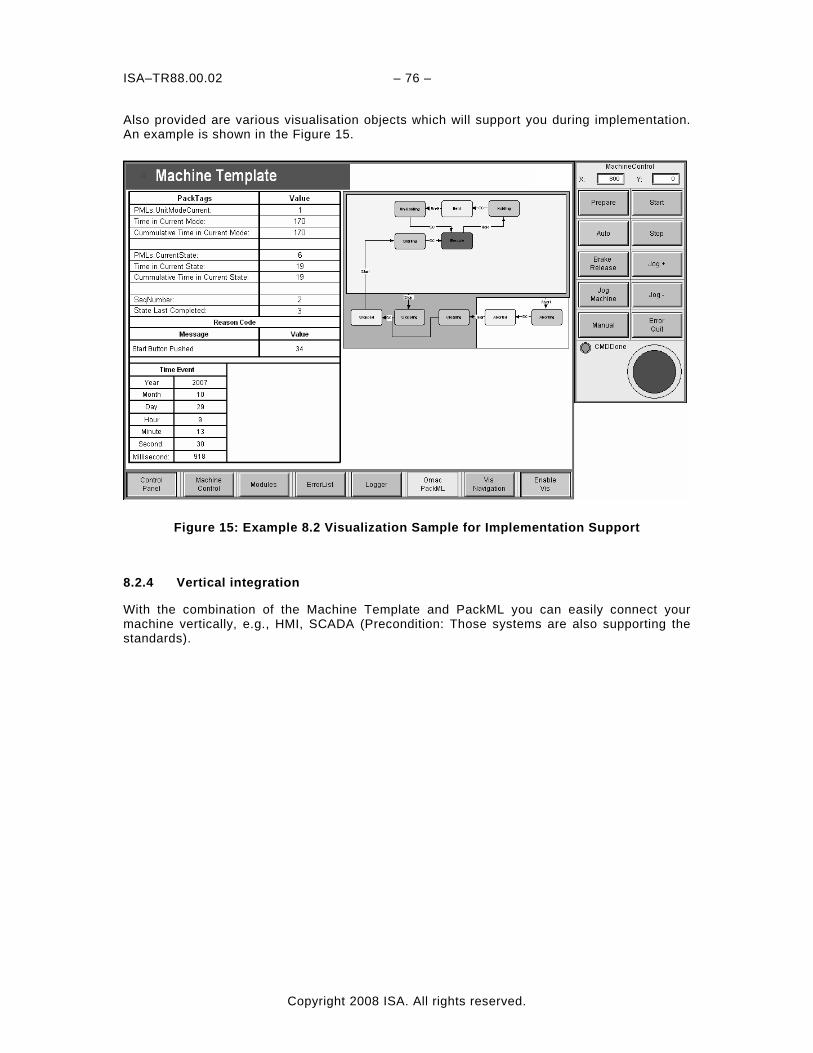
ISA–TR88.00.02 – 76 –


Also provided are various visualisation objects which will support you during implementation. An example is shown in the Figure 15.

Figure 15: Example 8.2 Visualization Sample for Implementation Support

8.2.4 Vertical integration

With the combination of the Machine Template and PackML you can easily connect your machine vertically, e.g., HMI, SCADA (Precondition: Those systems are also supporting the standards).

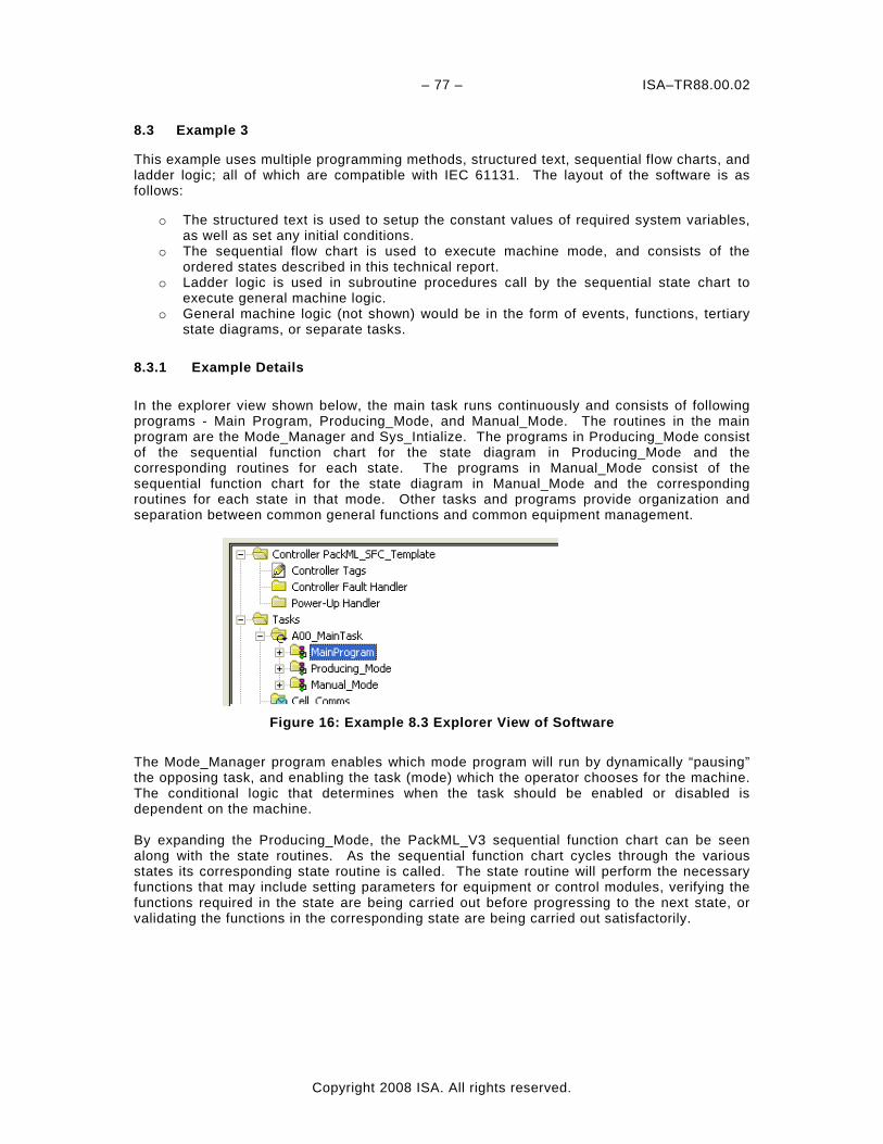
– 77 – ISA–TR88.00.02


8.3 Example 3

This example uses multiple programming methods, structured text, sequential flow charts, and ladder logic; all of which are compatible with IEC 61131. The layout of the software is as follows:

o The structured text is used to setup the constant values of required system variables, as well as set any initial conditions.

o The sequential flow chart is used to execute machine mode, and consists of the ordered states described in this technical report.

o Ladder logic is used in subroutine procedures call by the sequential state chart to execute general machine logic.

o General machine logic (not shown) would be in the form of events, functions, tertiary state diagrams, or separate tasks.

8.3.1 Example Details In the explorer view shown below, the main task runs continuously and consists of following programs - Main Program, Producing_Mode, and Manual_Mode. The routines in the main program are the Mode_Manager and Sys_Intialize. The programs in Producing_Mode consist of the sequential function chart for the state diagram in Producing_Mode and the corresponding routines for each state. The programs in Manual_Mode consist of the sequential function chart for the state diagram in Manual_Mode and the corresponding routines for each state in that mode. Other tasks and programs provide organization and separation between common general functions and common equipment management.

Figure 16: Example 8.3 Explorer View of Software

The Mode_Manager program enables which mode program will run by dynamically “pausing” the opposing task, and enabling the task (mode) which the operator chooses for the machine. The conditional logic that determines when the task should be enabled or disabled is dependent on the machine. By expanding the Producing_Mode, the PackML_V3 sequential function chart can be seen along with the state routines. As the sequential function chart cycles through the various states its corresponding state routine is called. The state routine will perform the necessary functions that may include setting parameters for equipment or control modules, verifying the functions required in the state are being carried out before progressing to the next state, or validating the functions in the corresponding state are being carried out satisfactorily.

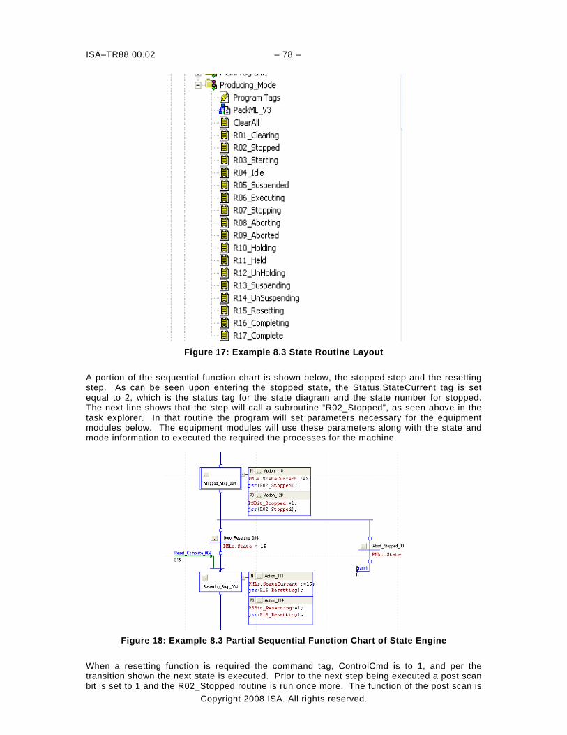
ISA–TR88.00.02 – 78 –


Figure 17: Example 8.3 State Routine Layout

A portion of the sequential function chart is shown below, the stopped step and the resetting step. As can be seen upon entering the stopped state, the Status.StateCurrent tag is set equal to 2, which is the status tag for the state diagram and the state number for stopped. The next line shows that the step will call a subroutine “R02_Stopped”, as seen above in the task explorer. In that routine the program will set parameters necessary for the equipment modules below. The equipment modules will use these parameters along with the state and mode information to executed the required the processes for the machine.

Figure 18: Example 8.3 Partial Sequential Function Chart of State Engine

When a resetting function is required the command tag, ControlCmd is to 1, and per the transition shown the next state is executed. Prior to the next step being executed a post scan bit is set to 1 and the R02_Stopped routine is run once more. The function of the post scan is

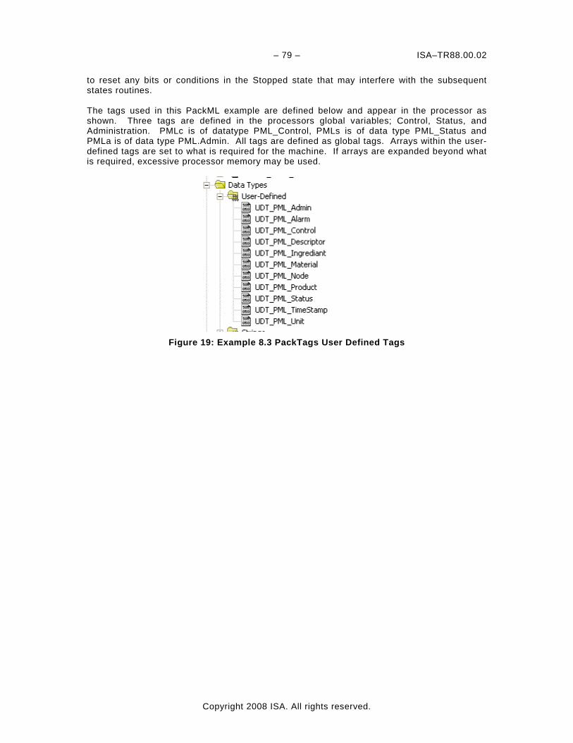
– 79 – ISA–TR88.00.02


to reset any bits or conditions in the Stopped state that may interfere with the subsequent states routines. The tags used in this PackML example are defined below and appear in the processor as shown. Three tags are defined in the processors global variables; Control, Status, and Administration. PMLc is of datatype PML_Control, PMLs is of data type PML_Status and PMLa is of data type PML.Admin. All tags are defined as global tags. Arrays within the user-defined tags are set to what is required for the machine. If arrays are expanded beyond what is required, excessive processor memory may be used.

Figure 19: Example 8.3 PackTags User Defined Tags

ISA–TR88.00.02 – 80 –


8.4 Example 4

8.4.1 Overview

To support implementation of PackML standards into machine control applications there are various software modules and templates available for the many different automation systems. Examples of the latest developments are as follows:

• Function Blocks provide a basis for unit mode selection and state handling of a machine. They represent a useful frame for the machine dependent application code, ensuring that mode and state management is realized according to PackML guidelines.

• Predefined data structures containing the complete range of PackTags ensure a fast and easy declaration of program variables for command, status, and administration signals.

. 8.4.2 Automation Templates

The Example Automation Templates, also called Libraries, delivers OMAC PackML solutions in the form of example control code and data areas. The control code consists of the Unit Mode Manager, Base State Model, the full PackTags data area, and other OMAC support code (Alarm Management, etc.). Furthermore, since these templates are programmed using our standard, modular programming techniques can be used on the newest machines or in retrofit applications. The control code is written in the IEC-61131 languages of Ladder Logic (LAD) & Structured Text (ST).

For the template below, the main folder contains the central logic and function calls for the machine. The “ModeMgr”, being this example’s version of the OMAC “Mode Management” routine, is used to control the machines’ Unit Control Mode. This template has three (3) Unit Control Modes: Cleaning Mode (“UC_Clean”), Maintenance Mode (“UC_Maint”), and Production Mode (“UC_Prod”). All of the Unit Control Modes are based upon the OMAC Base State Model. Each Unit Control Mode consists of its’ own individual State Functions. The Production Mode (“UC_Prod”), shown expanded, clearly shows the entire subset of states of the Base State Model (clearing, stopped, starting, etc.)

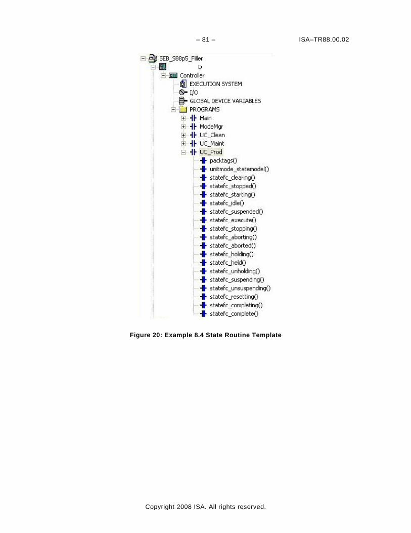
– 81 – ISA–TR88.00.02


Figure 20: Example 8.4 State Routine Template

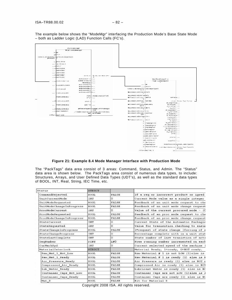
ISA–TR88.00.02 – 82 –


The example below shows the “ModeMgr” interfacing the Production Mode’s Base State Mode – both as Ladder Logic (LAD) Function Calls (FC’s).

Figure 21: Example 8.4 Mode Manager Interface with Production Mode

The “PackTags” data area consist of 3 areas: Command, Status, and Admin. The “Status” data area is shown below. The PackTags area consist of numerous data types, to include: Structures, Arrays, and User Defined Data Types (UDT’s), as well as the standard data types of BOOL, INT, Real, String, IEC Time, etc.

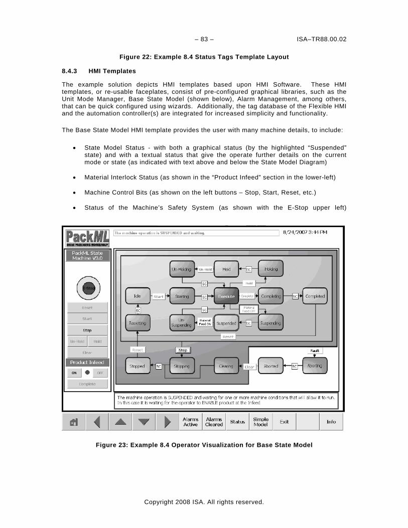
– 83 – ISA–TR88.00.02


Figure 22: Example 8.4 Status Tags Template Layout

8.4.3 HMI Templates

The example solution depicts HMI templates based upon HMI Software. These HMI templates, or re-usable faceplates, consist of pre-configured graphical libraries, such as the Unit Mode Manager, Base State Model (shown below), Alarm Management, among others, that can be quick configured using wizards. Additionally, the tag database of the Flexible HMI and the automation controller(s) are integrated for increased simplicity and functionality.

The Base State Model HMI template provides the user with many machine details, to include:

• State Model Status - with both a graphical status (by the highlighted “Suspended” state) and with a textual status that give the operate further details on the current mode or state (as indicated with text above and below the State Model Diagram)

• Material Interlock Status (as shown in the “Product Infeed” section in the lower-left)

• Machine Control Bits (as shown on the left buttons – Stop, Start, Reset, etc.)

• Status of the Machine’s Safety System (as shown with the E-Stop upper left)

Figure 23: Example 8.4 Operator Visualization for Base State Model

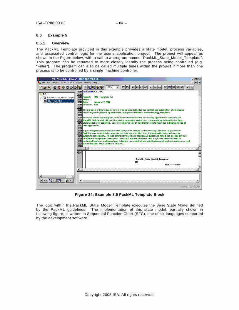
ISA–TR88.00.02 – 84 –


8.5 Example 5

8.5.1 Overview The PackML Template provided in this example provides a state model, process variables, and associated control logic for the user’s application project. The project will appear as shown in the Figure below, with a call to a program named “PackML_State_Model_Template”. This program can be renamed to more closely identify the process being controlled (e.g. “Filler”). The program can also be called multiple times within the project if more than one process is to be controlled by a single machine controller.

Figure 24: Example 8.5 PackML Template Block

The logic within the PackML_State_Model_Template executes the Base State Model defined by the PackML guidelines. The implementation of this state model, partially shown in following figure, is written in Sequential Function Chart (SFC), one of six languages supported by the development software.

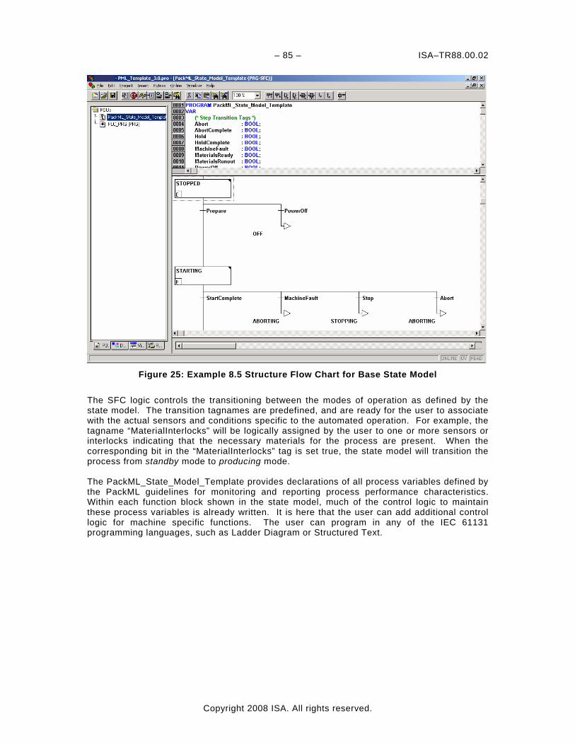
– 85 – ISA–TR88.00.02


Figure 25: Example 8.5 Structure Flow Chart for Base State Model

The SFC logic controls the transitioning between the modes of operation as defined by the state model. The transition tagnames are predefined, and are ready for the user to associate with the actual sensors and conditions specific to the automated operation. For example, the tagname “MaterialInterlocks” will be logically assigned by the user to one or more sensors or interlocks indicating that the necessary materials for the process are present. When the corresponding bit in the “MaterialInterlocks” tag is set true, the state model will transition the process from standby mode to producing mode. The PackML_State_Model_Template provides declarations of all process variables defined by the PackML guidelines for monitoring and reporting process performance characteristics. Within each function block shown in the state model, much of the control logic to maintain these process variables is already written. It is here that the user can add additional control logic for machine specific functions. The user can program in any of the IEC 61131 programming languages, such as Ladder Diagram or Structured Text.

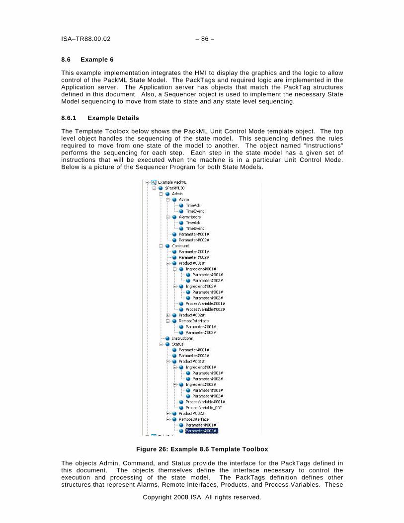
ISA–TR88.00.02 – 86 –


8.6 Example 6

This example implementation integrates the HMI to display the graphics and the logic to allow control of the PackML State Model. The PackTags and required logic are implemented in the Application server. The Application server has objects that match the PackTag structures defined in this document. Also, a Sequencer object is used to implement the necessary State Model sequencing to move from state to state and any state level sequencing.

8.6.1 Example Details

The Template Toolbox below shows the PackML Unit Control Mode template object. The top level object handles the sequencing of the state model. This sequencing defines the rules required to move from one state of the model to another. The object named “Instructions” performs the sequencing for each step. Each step in the state model has a given set of instructions that will be executed when the machine is in a particular Unit Control Mode. Below is a picture of the Sequencer Program for both State Models.

Figure 26: Example 8.6 Template Toolbox

The objects Admin, Command, and Status provide the interface for the PackTags defined in this document. The objects themselves define the interface necessary to control the execution and processing of the state model. The PackTags definition defines other structures that represent Alarms, Remote Interfaces, Products, and Process Variables. These

– 87 – ISA–TR88.00.02


structures are defined in objects that have the same name as the structure type. The definition allows for multiple copies of the structure to be used in the system. The example shows only two of each kind of object, but is capable of supporting any number of objects.

These templates are created and tested to verify their functionality works correctly. Then these templates can be used to make instances for each Unit or Supervisory system in the application. The templates are designed to allow quick and easy implementation without all the added work of I/O mapping and testing. These templates are designed to interact with the data from any available Unit according to the PackML guidelines.

The example is designed to be a Supervisory State Model. The templates are designed and will function as the Equipment State Model if necessary. Depending on your need for your project you can implement the solution without requiring the definition of a State Model in the machine controller.

Figure 27: Example 8.6 Sequencer Program for Automatic Mode State Model

8.6.2 Graphic Example

To provide the user of the equipment or system the capability to interact with the State Model, there are graphic symbols defined using the example program. These graphical symbols will work with the Application Server as shown in this example, but can also be used stand alone. Here is the graphical symbol for the State Model interface.

ISA–TR88.00.02 – 88 –


Figure 28: Example 8.6 Graphic Example of User Interface

Each state will change colour to indicate which state the system is running in. This diagram shows the colour of each state when it is active. The lighter shaded states are defined as a “Wait” state. The darker shaded states are defined as an “Acting” state. The “Execute” state is defined as a “Dual” state. The arrows with a label can be used to move from a “Wait” state to an “Acting” state.

The graphic below can be used to view and control the current execution of the State Model. The six buttons on the right allow control of the State Model. This object can be used instead of the graphic above. This example graphic only provides the six commands listed, but could be modified to include all nine commands if desired.

Figure 29: Example 8.6 Unit Control

– 89 – ISA–TR88.00.02


The graphic below is used to view the Parameter array structure. There can be any number of parameters and each parameter will have an ID, Name, Value, and Units of Measure. If desired this graphic could be expanded to show more than the 8 lines of information. The scroll bar at the right would allow the graphic to show more than the 8 lines of information.

Figure 30: Example 8.6 Parameter Array Structure

This graphic shows how the Product array structure might be viewed. There can be any number of products. Each product will have an ID, Process Variables, and Ingredients. There can be any number of Process Variables and Ingredients. Ingredients can have any number of parameters. This graphic could be expanded to show more than the 8 lines of information. The scroll bar at the right of each object allows the graphic to show more than the 8 pieces of information.

Figure 31: Example 8.6 Product Array Structure

ISA–TR88.00.02 – 90 –


9 OEE Implementation Examples

This example illustrates the use of PackTags in calculating OEE, Overal Equipment Effectiveness. The scope of this example is broken into four sections. The first section is to define OEE and explain the basic theory of OEE. The next two sections will show two different examples of how OEE could be calculated. One example will show how an HMI or machine controller could calculate a real-time OEE. The second example will show how a higher level system could perform a more complex historical OEE calculation. The last example is a PackTags OEE harmonization with the European DIN 8782 standard on Beverage Packaging Technology. 9.1 OEE Definition Overall Equipment Effectiveness (OEE) is a measure comparing how well manufacturing equipment is running compared to the ideal plant. The resulting measurement is expressed as the ratio of the actual output of the equipment divided by the maximum possible output of the equipment under ideal conditions. OEE is calculated by multiplying three independently measured values: Availability, Performance Rate, and Quality Rate. The fundamental OEE definition is defined as an availability ratio multiplied by a performance ratio multiplied by a quality ratio.

OEE = Availability x Performance x Quality

Where each component is defined as the following: Availability = Operating Time / Planned Production Time

Performance = Total Pieces / (Operating Time* Ideal Run Rate)

Quality = Good Pieces / Total Pieces OEE is often displayed as a waterfall object in which the major components of Availability, Performance, and Quality are displayed graphically. Losses are further subdivided into categories within the OEE sections.

Figure 39: OEE Waterfall Diagram

– 91 – ISA–TR88.00.02


9.1.1 Availability Definition Availability is defined as operating time divided by planned production time. The basic concept behind availability is to show the time the machine has been running divided by the time that the machine has been planned to run. Typical losses in this area are losses to unplanned maintenance, cleaning, changeovers, and breakdowns. Availability = Operating Time / Planned Production Time Operating Time is defined as the amount of time the machine has been attempting to produce parts. Planned Production Time is defined as the total amount of time the machine has been scheduled to run. The availability category is designed to capture the following losses:

1. Unplanned Maintenance 2. Breakdowns

a. Tooling Failures b. General Breakdowns c. Equipment Failure

3. Setup and Adjustments a. Setup/Changeover b. Operator Shortages c. Major Adjustments d. Warm-Up Time

4. Unable to Run Equipment a. Material Shortages b. Labor Shortages

9.1.2 Performance Definition Performance is defined as the total number of pieces on which the machine operated divided by the ideal production if a machine ran perfectly for the allocated amount of operating time. Performance = Total Pieces / (Operating Time* Ideal Run Rate) Total Pieces is defined as good pieces and bad pieces during the production run. This should be linked to the main consumed count of the machine. If a filler, this should be bottles into the filler. Operating Time is defined as the amount of time the machine has been attempting to produce parts. (Same as above) Ideal Run Rate is defined as the ideal rate that the machine can run for the product that is being run on the machine and the way the machine is configured. The performance category is designed to capture the following losses:

1. Small Stops a. Obstructed Product Flow b. Component Jams c. Misfeeds d. Sensor Blocked e. Delivery Blocked f. Cleaning/Checking

2. Reduced Speed

a. Rough Running b. Under Nameplate Capacity

ISA–TR88.00.02 – 92 –


c. Equipment Wear d. Operator Inefficiency

9.1.3 Quality Definition Quality is defined as the total number of good pieces divided by the total number of pieces on which the machine operated. Quality = Good Pieces / Total Pieces Good Pieces is defined as only good pieces processed during the production run. So this is the main production processed count of the machine. If a filler, this should be bottles out of the filler. Total Pieces includes good pieces and bad pieces during the production run. This should be linked to the main consumed count of the machine. If a filler, this should be bottles into the filler. This should be the same count as used in the performance definition. The quality category is designed to capture the following losses:

1. Startup Rejects a. Scrap b. Rework c. In-Process Damage d. In-Process Expiration e. Incorrect Assembly

2. Production Rejects a. Scrap b. Rework c. In-Process Damage d. In-Process Expiration e. Incorrect Assembly

9.2 Calculating a Real-Time OEE in a Machine Controller or HMI The first example is a simple real-time calculation based upon PackTags with data originating from the machine controller. This example will not require historical tracking of information and will show a calculation of OEE since the last time the machine counts and timers were reset in the machine controller. This example is recommended for machine builders and control vendors that want to show a basic OEE on their HMI systems. The limitation of this calculation will be that it will only be valid for the time period since the last time the counts and times were reset in the machine controller. It will also be invalid if the setup or product of the machine causes the design speed of the machine to change.

OEE = Availability x Performance x Quality 9.2.1 Availability Availability = Operating Time / Planned Production Time Planned Production Time is defined as the amount of time that the machine is scheduled to run production. This includes time such as changeover time, unplanned maintenance time, and major breakdowns. For this implementation, it will be assumed that the machine is always scheduled to run. The number of total seconds since the last reset occurred can be obtained using the following tag: UnitName.Admin.AccTimeSinceReset

Operating Time is defined as the time the machine has been attempting to run production. This should be linked to the time that the machine has been in production mode. The number of seconds in production mode since the last reset occurred can be typically obtained using the following tag: UnitName.Admin.ModeCumulativeTime[#] where the # is typically 1 for Producing Mode.

– 93 – ISA–TR88.00.02


9.2.2 Performance

Performance = Total Pieces / (Operating Time * Ideal Run Rate / 60)

Total Pieces is defined as the total pieces that have been brought into the machine from the primary production path. The number of units that have been brought into the machine since the last reset can typically be obtained through the following tag: UnitName.Admin.ProdProcessedCount[#].Count where the # is typically 1. Ideal Run Rate is defined as the maximum rate the machine can run given the current product and setup of the machine. This number may change based upon a product being run on the machine. Should this number change, then the OEE calculation will become invalid. It is suggested that if this number ever change, that a reset on the count and timers should occur. The number of units per minute for the ideal run rate can be obtained using the following tag: UnitName.Admin.MachDesignSpeed. NOTE: Because the unit of time for MachDesignSpeed is in minutes and the operating time is in seconds, there needs to be a unit correction factor in the above equation. We have chosen to divide the MachDesignSpeed by 60 to convert it into units per second. This will keep units consistent in the above equation.

9.2.3 Quality Quality = Good Pieces / Total Pieces Good Pieces – This includes only good pieces during the production run. This is the main production processed count of the machine. If a filler, this should be bottles out of the filler. The number of good pieces of production that have been run since the last count reset can be obtained by subtracting the total products processed minus the products that were defective: UnitName.Admin.ProdProcessedCount[#].Count - UnitName.Admin.ProdDefectiveCount[#].Count where the # is typically 0 for both counters as a default. If multiple products are being tracked the index may change. Total Pieces is defined as the total pieces that have been brought into the machine from the primary production path. The number of units that have been brought into the machine since the last reset can typically be obtained through the following tag: UnitName.Admin.ProdProcessedCount[#].Count where the # is typically 0 as a default. If multiple products are being tracked the index may change. 9.2.4 Overall Real-Time OEE Calculation When multiplying Availability, Performance, and Quality the following equation for OEE is produced:

UnitName.Admin.ProdProcessedCount[#].Count - UnitName.Admin.ProdDefectCount[#].Count UnitName.Admin.AccTimeSinceLastReset * UnitName.Admin.MachDesignSpeed / 60

OEE =

9.2.5 Limitations of Real-Time OEE Equation The above real-time OEE equation is only valid for the time period since the times and counts were last reset in the machine controller. It also becomes invalid if the MachDesignSpeed is ever changed. Should there be desire to compute a more detailed OEE equation or an OEE equation over a different time period, then please examine the second example that involves keeping track of historical data in a higher level system. 9.3 Calculating a Complex Historical OEE Using a Historical Database Based System This second example will assume a higher level system such as an OEE tracking system or an MES system has been installed and is capable of storing information into a database. The higher level system should also be capable of performing complex calculations. In this example, information will retrieved from the machine controller using PackTags, but will be stored and calculated in a higher level system. This example is recommended for advanced

ISA–TR88.00.02 – 94 –


users who need to analyze OEE over an arbitrary time period and who need to be detailed analysis of their OEE losses. OEE = Availability x Performance x Quality Availability = Operating Time / Planned Production Time Planned Production Time is defined as the amount of time that the machine is scheduled to run production. This includes time such as changeover time, unplanned maintenance time, and major breakdowns. It should subtract out time that the machine is not planned to run for such times as planned maintenance and curtailment. This time should come from a higher level planning system such as an MES or ERP system. Operating Time is defined as the amount of time the machine has been attempting to produce parts while the machine is scheduled to run production. This time should be computed in a higher level system by monitoring the following tags: UnitName.Status.UnitModeCurrent and the UnitName.Status.StateCurrent Through monitoring the above tags, a higher level system should keep track of the exact time that each of these tags change. By keeping track of the time that these tags change, a higher level system can compute the amount of operating time a machine has occurred. It is important to note that a higher level system should only compute the time for operating time while the machine is scheduled to run production. The periods of time the machine is scheduled to run production will need to be obtained from an MES or ERP system. Performance = Total Pieces / (Operating Time * Ideal Run Rate) Total Pieces includes good pieces and bad pieces during the production run. This should be linked to the main consumed count of the machine. If a filler, this should be bottles into the filler. This should come from the following tag:

UnitName.Admin.ProdProcessedCount[#].AccCount This value rolls over to 0 at the user defined maximum count of 2,147,483,647 and doesn’t reset. A higher level system should be continually monitoring this count and then storing the count delta at some interval period. An example of this would be to monitor this count and then to store the count delta every minute into a database. A higher level system could then use this information to compute an OEE count for an arbitrary time period. The resolution of storage will determine the resolution of accuracy on the boundary conditions of the times. Operating Time is defined in availability above and is the same equation. Ideal Run Rate is the ideal rate that the machine can run for the product that is being run on the machine and the way the machine is configured. This is read through the tag:

UnitName.Admin.MachDesignSpeed.

Because the ideal run rate changes over time based upon setup of the machine and the product that is currently being run, the value must be tracked in the higher level system every time it changes. Then the time weighted average of the MachDesignSpeed must be computed. It is important to only take into account the time periods for which the operating time is applied when computing the time weighted average for the ideal run rate. Quality =Good Pieces / Total Pieces Good Pieces includes only good pieces during the production run. This should be linked to the main produced count of the machine. If a filler, this should be bottles out of the filler. This should come from the following derivation:

– 95 – ISA–TR88.00.02


UnitName.Admin.ProdProcessedCount[#].AccCount - UnitName.Admin.ProdDefectiveCount[#].AccCount where, typically, the main cycle count or total number of products processed by the machine is indexed at 0 and the total number of culled or rejected products for the main path of the machine is also indexed at 0 for default products numbers. If multiple products are being tracked the index can vary. A higher level system should be continually executing this calculation and then storing the count delta at some interval period. An example of this would be to monitor these tag counts and then to store the resultant and continue to compute a delta every minute into a database. A higher level system could then use this information to compute an OEE count for an arbitrary time period. The resolution of storage will determine the resolution of accuracy on the boundary conditions of the times. Total Pieces is defined in the performance section above. It is very common for OEE analysis to divide quality losses between startup losses and non-startup losses. Should this be a concern, a higher level system can simply monitor the mode and state tags to determine the mode and state of the machine.

UnitName.Status.UnitModeCurrent and the UnitName.Status.StateCurrent By monitoring the two tags and defining the definition of startup losses, a higher level system can look at the counts above during the time period to determine startup losses. 9.3.1 Further Analysis of Performance It is extremely common to monitor the subcomponents of performance to try and understand the main causes for OEE loss in performance. The two most common losses to be monitored are low speed loss and small stop loses. This example will discuss how both of these losses can be further monitored using PackTags. 9.3.1.1 Low Speed Losses The current machine speed can be read through the tag UnitName.Status.CurMachSpeed and the designed speed for the machine for the current product and current setup is in the tag UnitName.Admin.MachDesignSpeed. Both of these tags can be monitored and their values can be stored in a database on a periodic basis. When computing a low speed loss, we can integrate these two curves over a given time period and then subtract the two. It is important to once again, only take into account the time the machine was accumulating operating time and the time that a small stop event was not occurring. 9.3.1.2 Small Stop Losses Small stop losses are one of the largest reasons for OEE losses and include such events as jams and material blockages. Automating the collection of small stop losses through a standard interface is one of the main value propositions of PackTags. Clause 9.3.1.3 describes the process by which information should be collected. 9.3.1.3 Mode or State Transition When a machine changes mode or state, we can monitor the state that the machine goes into and then capture all active alarms when the state transition occurred. While in production mode, it is important to track why the machine leaves Execute mode. In particular, it is good to know why a machine would go into Held, Suspended, Aborted or Stopped. By monitoring the following two tags, we can determine the current mode and the current state: UnitName.Status.UnitModeCurrent and the UnitName.Status.StateCurrent

ISA–TR88.00.02 – 96 –


Typically the UnitName.Status.UnitModeCurrent has a value of 1 when the machine is Producing mode and the UnitName.Status.StateCurrent has a value of 6 when the machine is executing. Whenever the transition from executing happens, the following algorithm should be run to determine the cause of the machine stoppage. 9.3.1.4 Loop through the Active Alarm File Through monitoring the Admin.Alarm[#] array, a program can determine the cause of the machine changing states if the state is automatically changed. This can be done by looking up the alarms that are active. If more than one alarm is active, then we can resolve the reason the machine stopped to the alarm that occurred most recently. This is done by looking at the time the state or mode transition occurred and then looking at the alarm file for the first event that occurred before the machine stopped. The following is an example determining a small stop cause:

1. A higher level system should be constantly scanning the fault array to have the current state of all currently occurring alarms. The higher level system will have the alarm state of all alarms prior to receive a state or mode transition.

2. When a machine transitions from Executing to Suspended because a jam sensor goes off,

the state status UnitName.Status.StateCurrent, goes from 6 to 13.

3. The higher level system receives the OPC change event from the OPC Server that the value of the status word changed from 6 to 13.

4. The higher level system should immediately perform a synchronous read of the alarm file to

read the entire alarm file.

5. The higher level system will compare the previous alarm file with the alarm file that was just read. Because the alarm file only contains active alarms and the alarm file is sorted in chronological order, the higher level system should be able to identify the alarm that caused the shutdown.

The reason we cannot just take the first alarm in the alarm file as a cause is because not all alarms may cause a state transition, although this is machine dependent. If a machine chooses to implement an Alarm file that only transitions the machine, then the above logic will work in that case as well. 9.3.2 Limitations of a Historical OEE Calculation If a higher level MES system or an OEE tracking system can save all of the data generated through a PackML interface, there are very few limitations that can be calculated using the above methods to determine OEE. It is recommended that a high speed OEE solution or high speed historian be used to accurately store all of the high speed high resolution values directly from the plant floor into a modern higher level system for analysis. The complexity is high for the above calculations, but is required for an accurate calculation of OEE and all of the areas of loss.

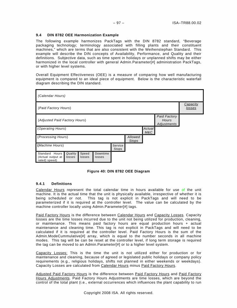
– 97 – ISA–TR88.00.02


9.4 DIN 8782 OEE Harmonization Example The following example harmonizes PackTags with the DIN 8782 standard, “Beverage packaging technology; terminology associated with filling plants and their constituent machines,” which are terms that are also consistent with the Weihenstephan Standard. This example will describe the DIN concepts of Availability, Performance, and Quality and their definitions. Subjective data, such as time spent in holidays or unplanned shifts may be either harmonized in the local controller with general Admin.Parameter[#] administration PackTags, or with higher level systems. Overall Equipment Effectiveness (OEE) is a measure of comparing how well manufacturing equipment is compared to an ideal piece of equipment. Below is the characteristic waterfall diagram describing the DIN standard.

(Calendar Hours)

(Paid Factory Hours) Capacity

losses

(Adjusted Paid Factory Hours) Paid Factory

Hours Adjustments

(Operating Hours)

Actual M&C

(Processing Hours)

Allowed Stops

(Machine Hours)

Service Stops

Standard Hours (Actual output at rated) speed)

Quality losses

Speed losses

Downtime losses

Figure 40: DIN 8782 OEE Diagram

9.4.1 Definitions Calendar Hours represent the total calendar time in hours available for use of the unit machine. It is the actual time that the unit is physically available, irrespective of whether it is being scheduled or not. This tag is not explicit in PackTags and will need to be parameterized if it is required at the controller level. The value can be calculated by the machine controller locally using Admin.Parameter[#] tags. Paid Factory Hours is the difference between Calendar Hours and Capacity Losses. Capacity losses are the time losses incurred due to the unit not being utilized for production, cleaning, or maintenance. This means paid factory hours are equal production hours + actual maintenance and cleaning time. This tag is not explicit in PackTags and will need to be calculated if it is required at the controller level. Paid Factory Hours is the sum of the Admin.ModeCummulative[#] array, which is equal to the number seconds in all machine modes. This tag will be can be reset at the controller level, if long term storage is required the tag can be moved to an Admin.Parameter[#] or to a higher level system. Capacity Losses: This is the time the unit is not utilized either for production or for maintenance and cleaning, because of agreed or legislated public holidays or company policy requirements (e.g., religious holidays, shifts not planned in either weekends or weekdays). Capacity Losses are calculated from Calendar Hours minus Paid Factory Hours. Adjusted Paid Factory Hours is the difference between Paid Factory Hours and Paid Factory Hours Adjustments. Paid Factory Hours Adjustments are time losses, which are beyond the control of the total plant (i.e., external occurrences which influences the plant capability to run

ISA–TR88.00.02 – 98 –


or produce). The value can be stored locally in the Admin.Parameter[#] or by the higher level system. Operating Hours are the difference between Adjusted Paid Factory Hours and Planned Maintenance and Cleaning Hours (M&C Hours). A recommended guideline for maintenance and cleaning as a percentage of paid factory hours is ±10 percent. When recording maintenance and cleaning, the actual time used for these activities, irrespective of whether the time falls in or out of the planned shift hours, and irrespective of who and how many people are used for maintenance and cleaning, should be recorded and reported. To track using PackTags the relative Admin.ModeCummulative[#] tags that are associated with cleaning and maintenance activities can be summed, and scaled. Processing Hours are the difference between Operating Hours and Allowed Stops. Allowed Stops are machine downtime allowances that result from specific operating requirements for a packaging line. These could be brand, pack, shift pattern, or technology related. The Allow Stops are based on the time the unit was stopped, however if the time taken to do a changeover is longer than the specified time, that actual time should be recorded against the machine. Allowed Stops are not tracked within PackTags. If Allowed Stops are to be tracked and Processing Hours calculated, stop codes may need to be examined and time spent for specific stops relating to downtime allowances will need to be accumulated and managed within Admin.Parameter[#] or the higher level system. Machine Hours are the difference between Processing Hours and Service Stops. Service stops are time lost on a unit due to factors that are external to the unit, but that are plant controllable. Service Stops are not tracked within PackTags. If Service Stops are to be tracked and Machine Hours calculated, stop codes may need to be examined and time spent for specific stops relating to downtime allowances will need to be accumulated and managed within Admin.Parameter[#] or the higher level system. Quality Loss is loss that is incurred when a unit produces poor quality products or the process is out of spec (impact on product quality) i.e., raw material quality/out of spec. problem. Examples of quality losses are as follows:

o Product rejects o Product rework o Frozen product that is not fit for commercial use sale o Stoppages due to the process or product that is not within the quality specification

Quality losses can be parameterized to time values by using the defective count divided by machine speed to calculate the time due to quality losses. PackTags use the tags Admin.ProdDefective[#] for defective products and Status.CurMachSpeed for the current machine speed.

Speed losses are performance related losses. Examples of speed losses are as follows:

o Rated speed variations o Machine ramp up and slow downs

Speed losses are normally recorded, but may be classified as “unidentified” or “unaccountable” if they are not fully assignable – usually calculated as the difference between the calculated stoppage time and the captured time. Speed losses can be parameterized in terms of proportional time as well by assuming the speed difference is lost product and therefore lost time. The quantity of Admin.MachDesignSpeed minus Status.CurMachSpeed divided by the time at Status.CurMachSpeed will yield the lost product opportunity. Using the lost product and dividing by the Admin.MachDesignSpeed will yield the lost machine time.

Standard Hours (Actual output at rated speed) is Actual Saleable Product (Units) / Rated Speed of the Line (Units/Hour). The Accumulated Actual Saleable time is Admin.ProdProcessedCount[#].AccCount – Admin.ProdDefectiveCount[#].AccCount. Rated Line Speed from PackTags is the Admin.MachDesignSpeed.

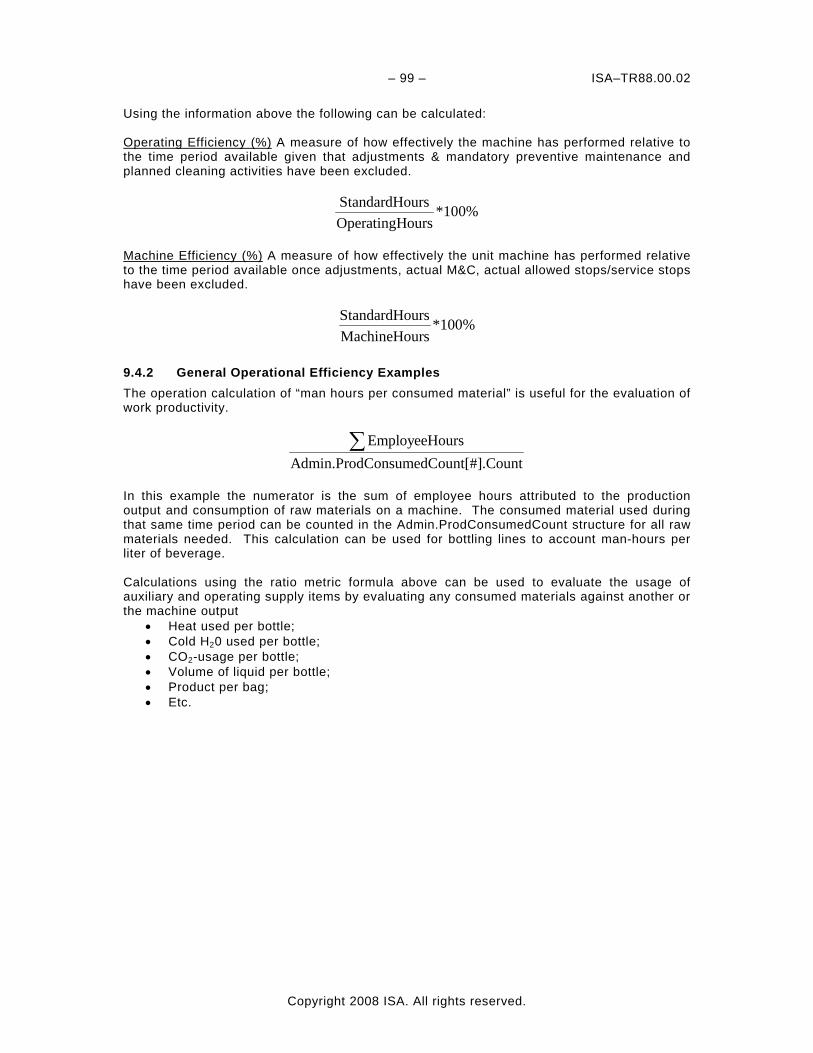
– 99 – ISA–TR88.00.02


Using the information above the following can be calculated: Operating Efficiency (%) A measure of how effectively the machine has performed relative to the time period available given that adjustments & mandatory preventive maintenance and planned cleaning activities have been excluded.

StandardHours *100%OperatingHours

Machine Efficiency (%) A measure of how effectively the unit machine has performed relative to the time period available once adjustments, actual M&C, actual allowed stops/service stops have been excluded.

StandardHours *100%MachineHours

9.4.2 General Operational Efficiency Examples The operation calculation of “man hours per consumed material” is useful for the evaluation of work productivity.

EmployeeHoursAdmin.ProdConsumedCount[#].Count

∑

In this example the numerator is the sum of employee hours attributed to the production output and consumption of raw materials on a machine. The consumed material used during that same time period can be counted in the Admin.ProdConsumedCount structure for all raw materials needed. This calculation can be used for bottling lines to account man-hours per liter of beverage. Calculations using the ratio metric formula above can be used to evaluate the usage of auxiliary and operating supply items by evaluating any consumed materials against another or the machine output

• Heat used per bottle; • Cold H20 used per bottle; • CO2-usage per bottle; • Volume of liquid per bottle; • Product per bag; • Etc.

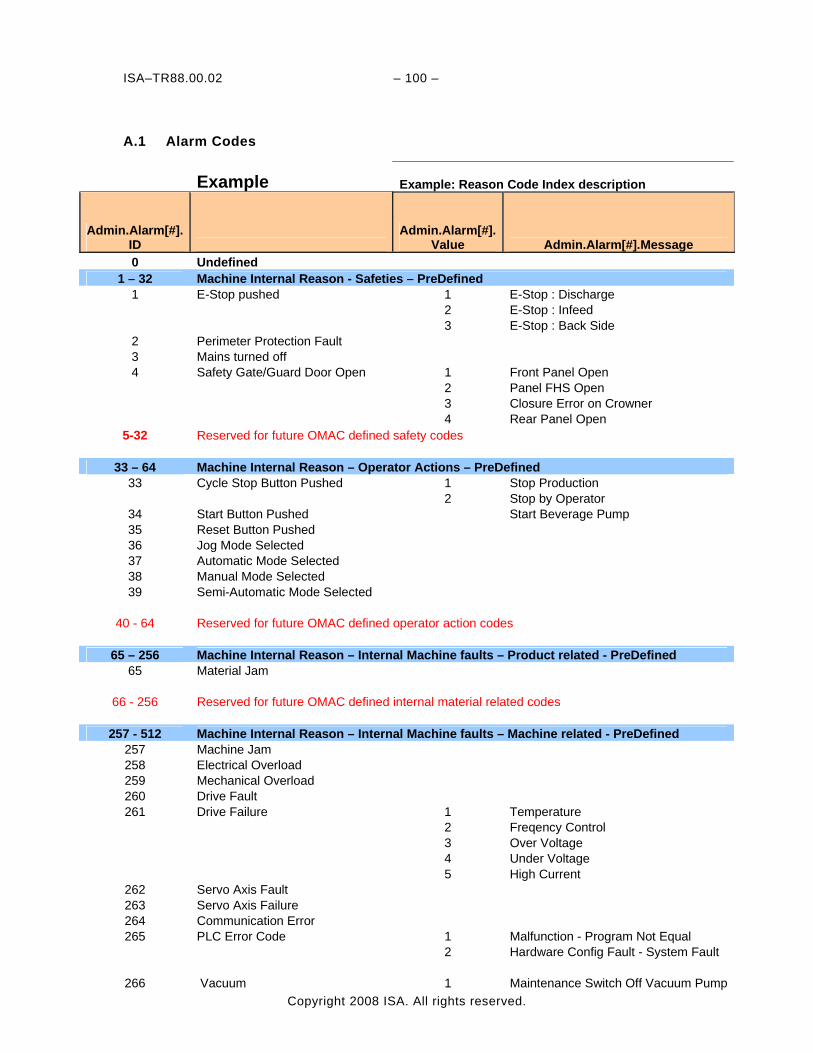
ISA–TR88.00.02 – 100 –


A.1 Alarm Codes

Example Example: Reason Code Index description

Admin.Alarm[#]. ID

Admin.Alarm[#].Value Admin.Alarm[#].Message

0 Undefined 1 – 32 Machine Internal Reason - Safeties – PreDefined

1 E-Stop pushed 1 E-Stop : Discharge 2 E-Stop : Infeed 3 E-Stop : Back Side 2 Perimeter Protection Fault 3 Mains turned off 4 Safety Gate/Guard Door Open 1 Front Panel Open 2 Panel FHS Open 3 Closure Error on Crowner 4 Rear Panel Open

5-32 Reserved for future OMAC defined safety codes

33 – 64 Machine Internal Reason – Operator Actions – PreDefined 33 Cycle Stop Button Pushed 1 Stop Production 2 Stop by Operator

34 Start Button Pushed Start Beverage Pump 35 Reset Button Pushed 36 Jog Mode Selected 37 Automatic Mode Selected 38 Manual Mode Selected 39 Semi-Automatic Mode Selected

40 - 64 Reserved for future OMAC defined operator action codes

65 – 256 Machine Internal Reason – Internal Machine faults – Product related - PreDefined 65 Material Jam

66 - 256 Reserved for future OMAC defined internal material related codes

257 - 512 Machine Internal Reason – Internal Machine faults – Machine related - PreDefined 257 Machine Jam 258 Electrical Overload 259 Mechanical Overload 260 Drive Fault 261 Drive Failure 1 Temperature

2 Freqency Control 3 Over Voltage 4 Under Voltage 5 High Current

262 Servo Axis Fault 263 Servo Axis Failure 264 Communication Error 265 PLC Error Code 1 Malfunction - Program Not Equal

2 Hardware Config Fault - System Fault

266 Vacuum 1 Maintenance Switch Off Vacuum Pump

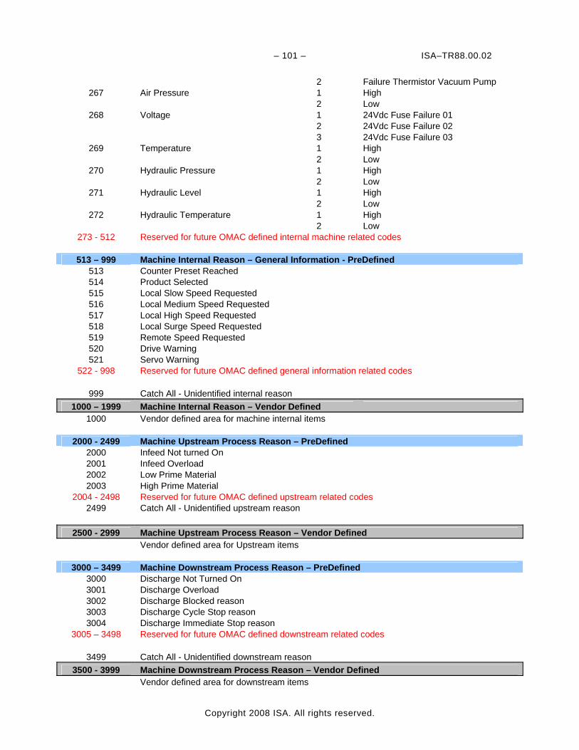
– 101 – ISA–TR88.00.02


2 Failure Thermistor Vacuum Pump 267 Air Pressure 1 High

2 Low 268 Voltage 1 24Vdc Fuse Failure 01

2 24Vdc Fuse Failure 02 3 24Vdc Fuse Failure 03

269 Temperature 1 High 2 Low

270 Hydraulic Pressure 1 High 2 Low

271 Hydraulic Level 1 High 2 Low

272 Hydraulic Temperature 1 High 2 Low

273 - 512 Reserved for future OMAC defined internal machine related codes

513 – 999 Machine Internal Reason – General Information - PreDefined 513 Counter Preset Reached 514 Product Selected 515 Local Slow Speed Requested 516 Local Medium Speed Requested 517 Local High Speed Requested 518 Local Surge Speed Requested 519 Remote Speed Requested 520 Drive Warning 521 Servo Warning

522 - 998 Reserved for future OMAC defined general information related codes

999 Catch All - Unidentified internal reason 1000 – 1999 Machine Internal Reason – Vendor Defined

1000 Vendor defined area for machine internal items

2000 - 2499 Machine Upstream Process Reason – PreDefined 2000 Infeed Not turned On 2001 Infeed Overload 2002 Low Prime Material 2003 High Prime Material

2004 - 2498 Reserved for future OMAC defined upstream related codes 2499 Catch All - Unidentified upstream reason

2500 - 2999 Machine Upstream Process Reason – Vendor Defined

Vendor defined area for Upstream items

3000 – 3499 Machine Downstream Process Reason – PreDefined 3000 Discharge Not Turned On 3001 Discharge Overload 3002 Discharge Blocked reason 3003 Discharge Cycle Stop reason 3004 Discharge Immediate Stop reason

3005 – 3498 Reserved for future OMAC defined downstream related codes

3499 Catch All - Unidentified downstream reason 3500 - 3999 Machine Downstream Process Reason – Vendor Defined

Vendor defined area for downstream items

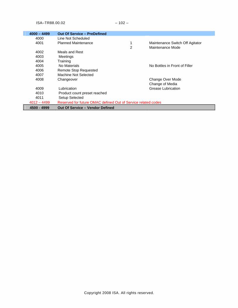
ISA–TR88.00.02 – 102 –


4000 – 4499 Out Of Service – PreDefined 4000 Line Not Scheduled 4001 Planned Maintenance 1 Maintenance Switch Off Agitator

2 Maintenance Mode 4002 Meals and Rest 4003 Meetings 4004 Training 4005 No Materials No Bottles in Front of Filler 4006 Remote Stop Requested 4007 Machine Not Selected 4008 Changeover Change Over Mode

Change of Media 4009 Lubrication Grease Lubrication 4010 Product count preset reached 4011 Setup Selected

4012 – 4499 Reserved for future OMAC defined Out of Service related codes 4500 - 4999 Out Of Service – Vendor Defined

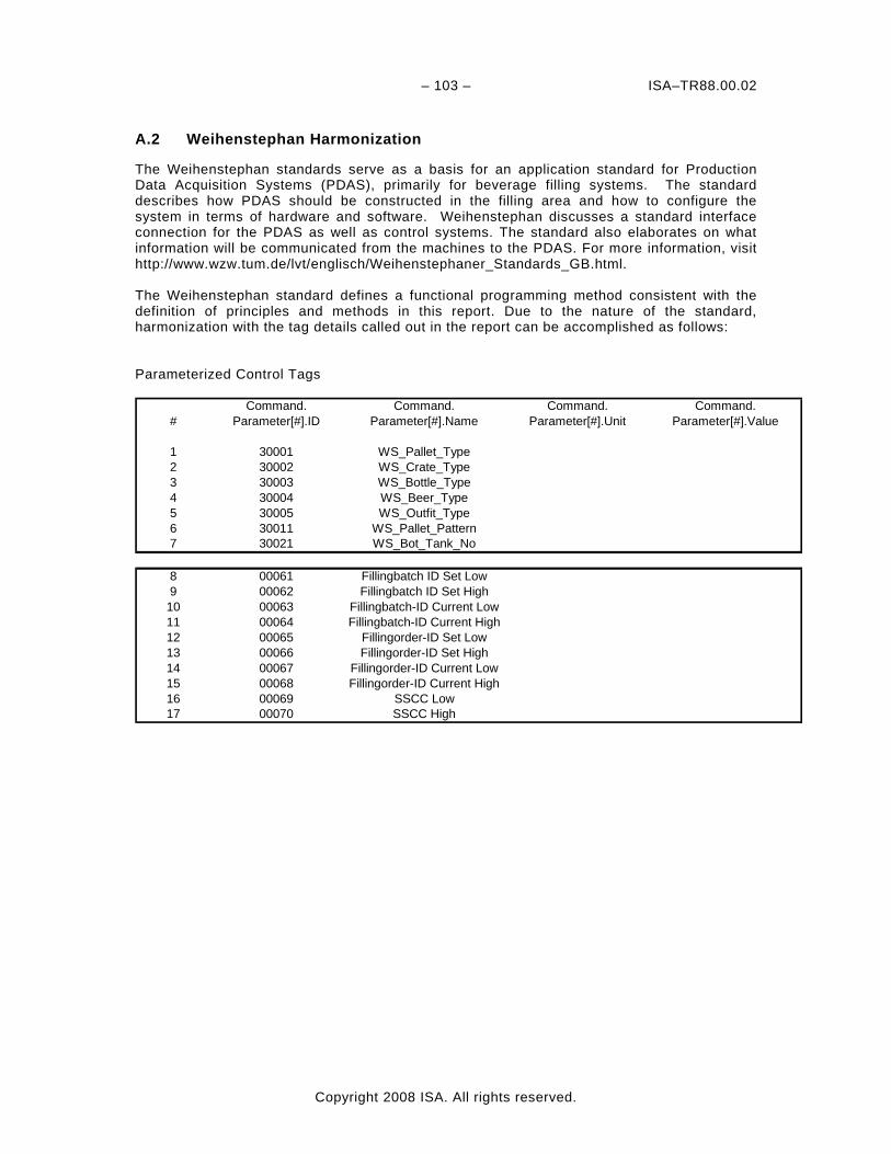
– 103 – ISA–TR88.00.02


A.2 Weihenstephan Harmonization

The Weihenstephan standards serve as a basis for an application standard for Production Data Acquisition Systems (PDAS), primarily for beverage filling systems. The standard describes how PDAS should be constructed in the filling area and how to configure the system in terms of hardware and software. Weihenstephan discusses a standard interface connection for the PDAS as well as control systems. The standard also elaborates on what information will be communicated from the machines to the PDAS. For more information, visit http://www.wzw.tum.de/lvt/englisch/Weihenstephaner_Standards_GB.html. The Weihenstephan standard defines a functional programming method consistent with the definition of principles and methods in this report. Due to the nature of the standard, harmonization with the tag details called out in the report can be accomplished as follows: Parameterized Control Tags

Command. Command. Command. Command.# Parameter[#].ID Parameter[#].Name Parameter[#].Unit Parameter[#].Value

1 30001 WS_Pallet_Type2 30002 WS_Crate_Type3 30003 WS_Bottle_Type4 30004 WS_Beer_Type5 30005 WS_Outfit_Type6 30011 WS_Pallet_Pattern7 30021 WS_Bot_Tank_No

8 00061 Fillingbatch ID Set Low9 00062 Fillingbatch ID Set High10 00063 Fillingbatch-ID Current Low11 00064 Fillingbatch-ID Current High12 00065 Fillingorder-ID Set Low13 00066 Fillingorder-ID Set High14 00067 Fillingorder-ID Current Low15 00068 Fillingorder-ID Current High16 00069 SSCC Low17 00070 SSCC High

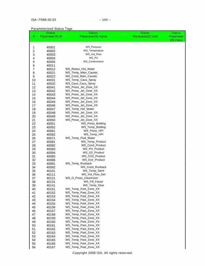
ISA–TR88.00.02 – 104 –


Parameterized Status Tags Status. Status. Status. Status. # Parameter[#].ID Parameter[#].Name Parameter[#].Unit Parameter

[#].Value 1 40001 WS_Pressure 2 40002 WS_Temperature 3 40003 WS_Vol_Flow 4 40004 WS_PU 5 40005 WS_Conductance 6 40011 7 40012 WS_Redox_Hot_Water 8 40021 WS_Temp_Main_Caustic 9 40022 WS_Cond_Main_Caustic

10 40031 WS_Temp_Caus_Spray 11 40032 WS_Caus_Caus_Spray 12 40041 WS_Press_Jet_Zone_XX 13 40042 WS_Press_Jet_Zone_XX 14 40043 WS_Press_Jet_Zone_XX 15 40044 WS_Press_Jet_Zone_XX 16 40045 WS_Press_Jet_Zone_XX 17 40046 WS_Press_Jet_Zone_XX 18 40047 WS_Temp_Hot_Water 19 40048 WS_Press_Jet_Zone_XX 20 40049 WS_Press_Jet_Zone_XX 21 40050 WS_Press_Jet_Zone_XX 22 40051 WS_Press_Bottling 23 40052 WS_Temp_Bottling 24 40061 WS_Press_HPI 25 40062 WS_Temp_HPI 26 40071 WS_Temp_Flod_Water 27 40081 WS_Temp_Product 28 40082 WS_Cond_Product 29 40083 WS_PH_Product 30 40084 WS_O2_Product 31 40085 WS_CO2_Product 32 40086 WS_Extr_Product 33 40091 WS_Temp_Runback 34 40092 WS_Cond_Runback 35 40101 WS_Temp_Steril 36 40111 WS_Vol_Flow_Det 37 40121 WS_O_Press_Cleanroom 38 40131 WS_Fill_Factor 39 40141 WS_Temp_Glue 40 40151 WS_Temp_Past_Zone_XX 41 40152 WS_Temp_Past_Zone_XX 42 40153 WS_Temp_Past_Zone_XX 43 40154 WS_Temp_Past_Zone_XX 44 40155 WS_Temp_Past_Zone_XX 45 40156 WS_Temp_Past_Zone_XX 46 40157 WS_Temp_Past_Zone_XX 47 40158 WS_Temp_Past_Zone_XX 48 40159 WS_Temp_Past_Zone_XX 49 40160 WS_Temp_Past_Zone_XX 50 40161 WS_Temp_Past_Zone_XX 51 40162 WS_Temp_Past_Zone_XX 52 40163 WS_Temp_Past_Zone_XX 53 40164 WS_Temp_Past_Zone_XX 54 40165 WS_Temp_Past_Zone_XX 55 40166 WS_Temp_Past_Zone_XX 56 40167 WS_Temp_Past_Zone_XX

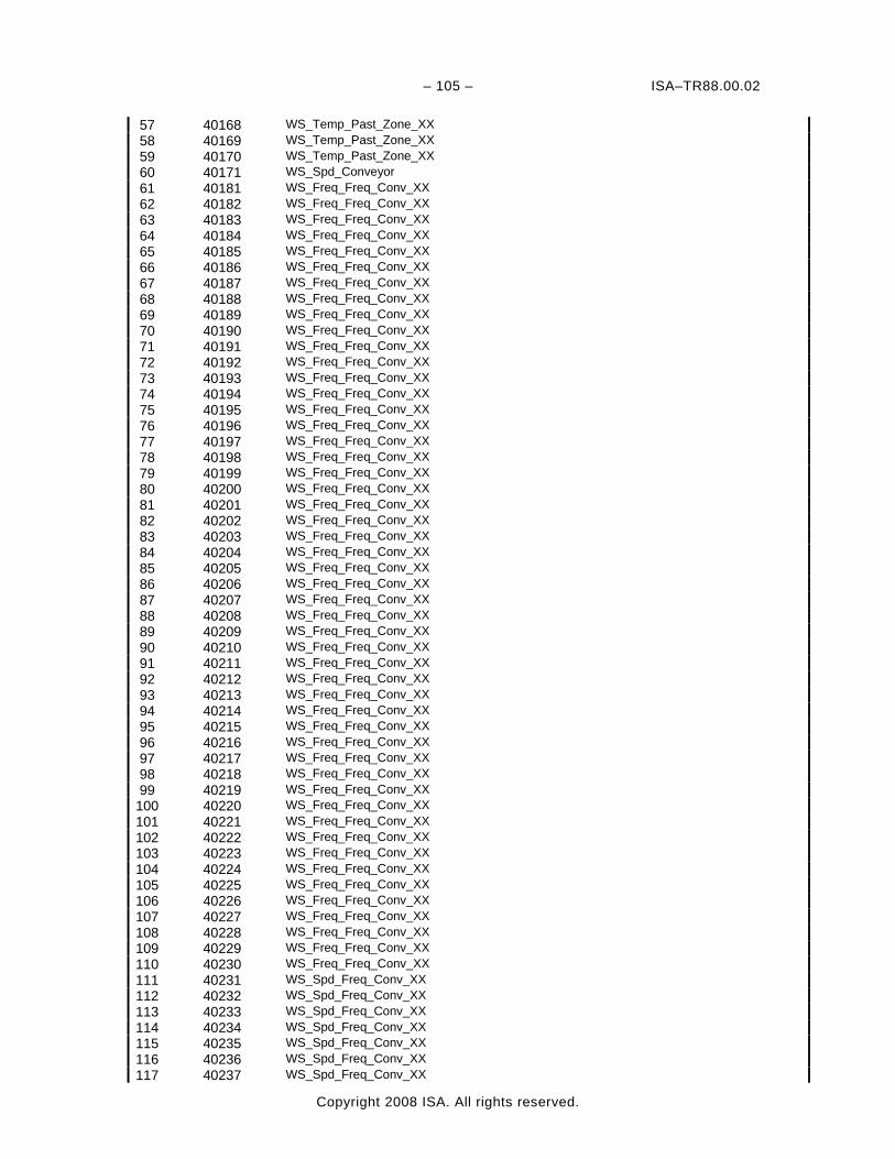
– 105 – ISA–TR88.00.02


57 40168 WS_Temp_Past_Zone_XX 58 40169 WS_Temp_Past_Zone_XX 59 40170 WS_Temp_Past_Zone_XX 60 40171 WS_Spd_Conveyor 61 40181 WS_Freq_Freq_Conv_XX 62 40182 WS_Freq_Freq_Conv_XX 63 40183 WS_Freq_Freq_Conv_XX 64 40184 WS_Freq_Freq_Conv_XX 65 40185 WS_Freq_Freq_Conv_XX 66 40186 WS_Freq_Freq_Conv_XX 67 40187 WS_Freq_Freq_Conv_XX 68 40188 WS_Freq_Freq_Conv_XX 69 40189 WS_Freq_Freq_Conv_XX 70 40190 WS_Freq_Freq_Conv_XX 71 40191 WS_Freq_Freq_Conv_XX 72 40192 WS_Freq_Freq_Conv_XX 73 40193 WS_Freq_Freq_Conv_XX 74 40194 WS_Freq_Freq_Conv_XX 75 40195 WS_Freq_Freq_Conv_XX 76 40196 WS_Freq_Freq_Conv_XX 77 40197 WS_Freq_Freq_Conv_XX 78 40198 WS_Freq_Freq_Conv_XX 79 40199 WS_Freq_Freq_Conv_XX 80 40200 WS_Freq_Freq_Conv_XX 81 40201 WS_Freq_Freq_Conv_XX 82 40202 WS_Freq_Freq_Conv_XX 83 40203 WS_Freq_Freq_Conv_XX 84 40204 WS_Freq_Freq_Conv_XX 85 40205 WS_Freq_Freq_Conv_XX 86 40206 WS_Freq_Freq_Conv_XX 87 40207 WS_Freq_Freq_Conv_XX 88 40208 WS_Freq_Freq_Conv_XX 89 40209 WS_Freq_Freq_Conv_XX 90 40210 WS_Freq_Freq_Conv_XX 91 40211 WS_Freq_Freq_Conv_XX 92 40212 WS_Freq_Freq_Conv_XX 93 40213 WS_Freq_Freq_Conv_XX 94 40214 WS_Freq_Freq_Conv_XX 95 40215 WS_Freq_Freq_Conv_XX 96 40216 WS_Freq_Freq_Conv_XX 97 40217 WS_Freq_Freq_Conv_XX 98 40218 WS_Freq_Freq_Conv_XX 99 40219 WS_Freq_Freq_Conv_XX

100 40220 WS_Freq_Freq_Conv_XX 101 40221 WS_Freq_Freq_Conv_XX 102 40222 WS_Freq_Freq_Conv_XX 103 40223 WS_Freq_Freq_Conv_XX 104 40224 WS_Freq_Freq_Conv_XX 105 40225 WS_Freq_Freq_Conv_XX 106 40226 WS_Freq_Freq_Conv_XX 107 40227 WS_Freq_Freq_Conv_XX 108 40228 WS_Freq_Freq_Conv_XX 109 40229 WS_Freq_Freq_Conv_XX 110 40230 WS_Freq_Freq_Conv_XX 111 40231 WS_Spd_Freq_Conv_XX 112 40232 WS_Spd_Freq_Conv_XX 113 40233 WS_Spd_Freq_Conv_XX 114 40234 WS_Spd_Freq_Conv_XX 115 40235 WS_Spd_Freq_Conv_XX 116 40236 WS_Spd_Freq_Conv_XX 117 40237 WS_Spd_Freq_Conv_XX

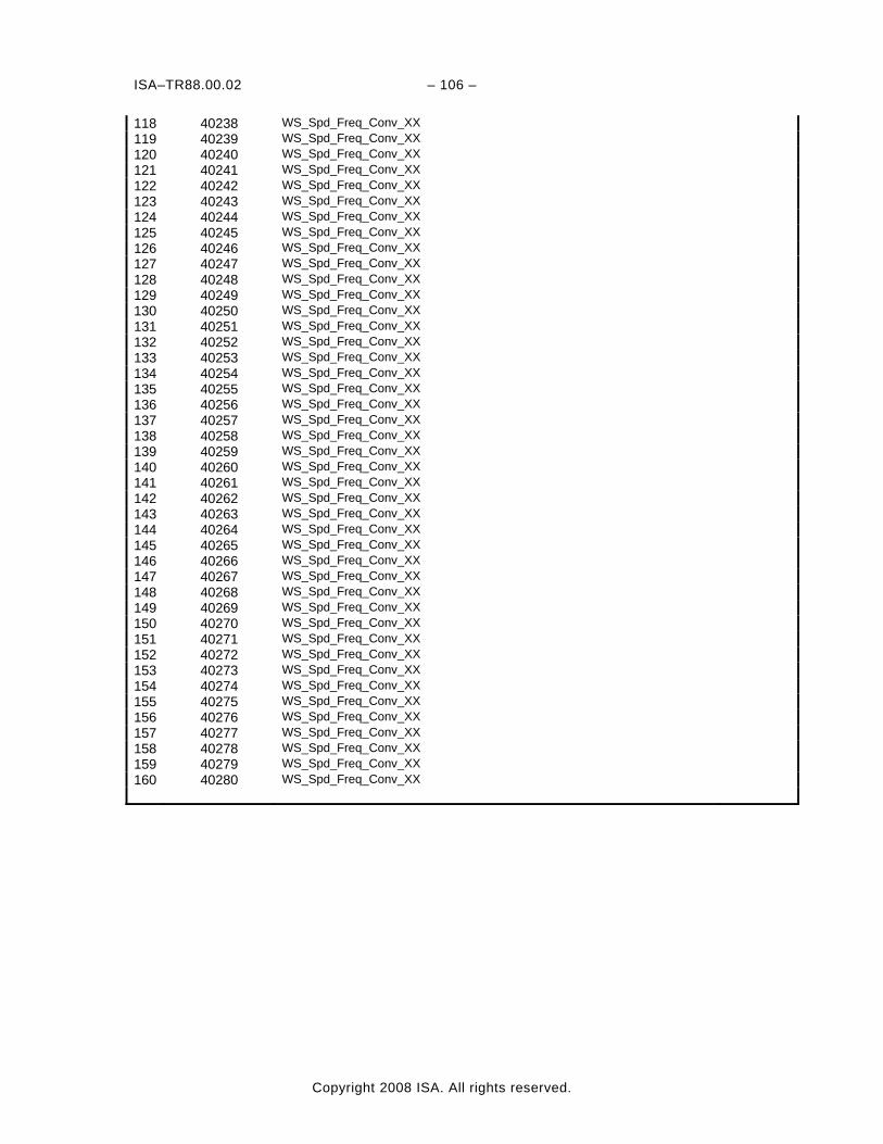
ISA–TR88.00.02 – 106 –


118 40238 WS_Spd_Freq_Conv_XX 119 40239 WS_Spd_Freq_Conv_XX 120 40240 WS_Spd_Freq_Conv_XX 121 40241 WS_Spd_Freq_Conv_XX 122 40242 WS_Spd_Freq_Conv_XX 123 40243 WS_Spd_Freq_Conv_XX 124 40244 WS_Spd_Freq_Conv_XX 125 40245 WS_Spd_Freq_Conv_XX 126 40246 WS_Spd_Freq_Conv_XX 127 40247 WS_Spd_Freq_Conv_XX 128 40248 WS_Spd_Freq_Conv_XX 129 40249 WS_Spd_Freq_Conv_XX 130 40250 WS_Spd_Freq_Conv_XX 131 40251 WS_Spd_Freq_Conv_XX 132 40252 WS_Spd_Freq_Conv_XX 133 40253 WS_Spd_Freq_Conv_XX 134 40254 WS_Spd_Freq_Conv_XX 135 40255 WS_Spd_Freq_Conv_XX 136 40256 WS_Spd_Freq_Conv_XX 137 40257 WS_Spd_Freq_Conv_XX 138 40258 WS_Spd_Freq_Conv_XX 139 40259 WS_Spd_Freq_Conv_XX 140 40260 WS_Spd_Freq_Conv_XX 141 40261 WS_Spd_Freq_Conv_XX 142 40262 WS_Spd_Freq_Conv_XX 143 40263 WS_Spd_Freq_Conv_XX 144 40264 WS_Spd_Freq_Conv_XX 145 40265 WS_Spd_Freq_Conv_XX 146 40266 WS_Spd_Freq_Conv_XX 147 40267 WS_Spd_Freq_Conv_XX 148 40268 WS_Spd_Freq_Conv_XX 149 40269 WS_Spd_Freq_Conv_XX 150 40270 WS_Spd_Freq_Conv_XX 151 40271 WS_Spd_Freq_Conv_XX 152 40272 WS_Spd_Freq_Conv_XX 153 40273 WS_Spd_Freq_Conv_XX 154 40274 WS_Spd_Freq_Conv_XX 155 40275 WS_Spd_Freq_Conv_XX 156 40276 WS_Spd_Freq_Conv_XX 157 40277 WS_Spd_Freq_Conv_XX 158 40278 WS_Spd_Freq_Conv_XX 159 40279 WS_Spd_Freq_Conv_XX 160 40280 WS_Spd_Freq_Conv_XX

– 107 – ISA–TR88.00.02


Parameterized Adminstration Tags Admin. Admin. Admin. Admin. # Parameter[#].ID Parameter[#].Name Parameter[#].Unit Parameter[#].Value 1 50001 WS_Tot_Pallets 2 50002 WS_Tot_Crates 3 50003 WS_Tot_Crates_Full 4 50004 WS_Tot_Crates_Empty 5 50005 WS_Tot_Bottles 6 50006 WS_Good_Bottles 7 50007 WS_Dis_Bott_Cont 8 50008 WS_Dis_Bott_Return 9 50009 WS_Burst_Bottles 10 50010 WS_Label 11 50011 WS_Tot_Rej 12 50012 WS_Rej_Wrong_Bottle 13 50013 WS_Rej_Bottle_High 14 50014 WS_Rej_Bottle_Low 15 50015 WS_Rej_Bottle_Colour 16 50016 WS_Rej_Def_Opening 17 50017 WS_Rej_Def_Botton 18 50018 WS_Rej_Scuffing 19 50019 WS_Rej_Bottle_Closed 20 50020 WS_Rej_Caustic 21 50021 WS_Rej_Foreign_Obj 22 50022 WS_Rej_Bottle_Under 23 50023 WS_Rej_Bottle_Over 24 50024 WS_Rej_Bottle_Clos 25 50025 WS_Rej_Date_Coding 26 50026 WS_Rej_Label_Fault 27 50027 WS_Rej_Crate_Defect 28 50028 WS_Rej_Crate_Colour 29 50029 WS_Rej_Crate_Logo 30 50030 WS_Rej_Comp_Empty

31-100 50031-50100 OTHER REJECT CAUSES 101 50101 WS_Cons_Clean_Water 102 50102 WS_Cons_Hot_Water 103 50103 WS_Cons_Steam 104 50104 WS_Cons_Sterile_Air 105 50105 WS_Cons_CO2 106 50106 WS_Cons_Detergents 107 50107 WS_Cons_Additives 108 50108 WS_Cons_Lubricant

109-150 50109-50150 OTHER CONSUMPTIONS 151 50151 WS_Tot_Crates_Bad 152 50152 WS_Bad_Cr_Miss_Bott 153 50153 WS_Bad_Cr_High_Bott 154 50154 WS_Bad_Cr_Low_Bott 155 50155 WS_Bad_Cr_Colour 156 50156 WS_Bad_Cr_Def_Handle

157-200 50157-50200 OTHER REASONS BAD CRATES 201 50201 WS_Pallets_Not_Comp 202 50202 WS_Def_Pallets 203 50203 WS_Not_Def_Pallets 204 50211 WS_Quantity_Product

ISA–TR88.00.02 – 108 –


205 50212 WS_Prod_Flow_Rate 206-905 50301-50999 WS_Fill_Valve_XXX_YYY

ISA–TR88.00.02 – 109 –


This page intentionally left blank.

Developing and promulgating sound consensus standards, recommended practices, and technical reports is one of ISA’s primary goals. To achieve this goal the Standards and Practices Department relies on the technical expertise and efforts of volunteer committee members, chairmen and reviewers. ISA is an American National Standards Institute (ANSI) accredited organization. ISA administers United States Technical Advisory Groups (USTAGs) and provides secretariat support for International Electrotechnical Commission (IEC) and International Organization for Standardization (ISO) committees that develop process measurement and control standards. To obtain additional information on the Society’s standards program, please write: ISA

Attn: Standards Department P.O. Box 12277 Research Triangle Park, NC 27709

ISBN: 978-1-934394-81-6

MAchine and Unite States Implementation

Documents

Transcript of MAchine and Unite States Implementation