MA, AR and ARMA Matthieu Stigler November 14, 2008...

Stationary modelsMA, AR and ARMA

Matthieu Stigler

November 14, 2008

Version 1.1

This document is released under the Creative Commons Attribution-Noncommercial 2.5 India

license.

Matthieu Stigler () Stationary models November 14, 2008 1 / 65

http://creativecommons.org/licenses/by-nc/2.5/in/

http://creativecommons.org/licenses/by-nc/2.5/in/

Lectures list

1 Stationarity

2 ARMA models for stationary variables

3 Seasonality

4 Non-stationarity

5 Non-linearities

6 Multivariate models

7 Structural VAR models

8 Cointegration the Engle and Granger approach

9 Cointegration 2: The Johansen Methodology

10 Multivariate Nonlinearities in VAR models

11 Multivariate Nonlinearities in VECM models


Outline

1 Last Lecture

2 AR(p) modelsAutocorrelation of AR(1)Stationarity ConditionsEstimation

3 MA modelsARMA(p,q)The Box-Jenkins approach

4 Forecasting


Recall: auto-covariance

Definition (autocovariance)

Cov(Xt ,Xt−k) ≡ γk(t) ≡ E [(Xt − µ)(Xt−k − µ)]

Definition (Autocorrelation)

Corr(Xt ,Xt−k) ≡ ρk(t) ≡ Cov(Xt ,Xt−k )Var(Xt)

Proposition

Corr(Xt ,Xt−0) = Var(Xt)

Corr(Xt ,Xt−j) = φj depend on the lage: plot its values at each lag.


Recall: stationarity

The stationarity is an essential property to define a time series process:

Definition

A process is said to be covariance-stationary, or weakly stationary, ifits first and second moments are time invariant.

E(Yt) = E[Yt−1] = µ ∀ tVar(Yt) = γ0 <∞ ∀ tCov(Yt ,Yt−k) = γk ∀ t, ∀ k


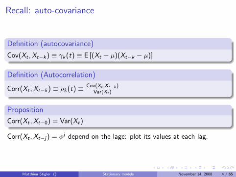
Recall: The AR(1)

The AR(1): Yt = c + ϕYt−1 + εt εt ∼ iid(0, σ2)with |ϕ| < 1, it can be can be written as:

Yt =c

1− ϕ+

t−1∑i=0

ϕiεt−i

Its ’moments’ do not depend on the time: :

E(Xt) = c1−ϕ

Var(Xt) = σ2

1−ϕ2

Cov(Xt ,Xt−j) = ϕj

1−ϕ2σ2

Corr(Xt ,Xt−j) = φj


Outline

1 Last Lecture



4 Forecasting


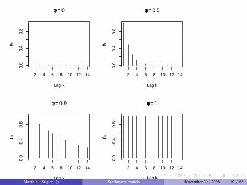
Autocorrelation function

A usefull plot to understand the dynamic of a process is theautocorrelation function:Plot the autocorrelation value for different lags.


2 4 6 8 10 12 14

0.0

0.4

0.8

Lag k

ρρ kφφ == 0

2 4 6 8 10 12 14

0.0

0.4

0.8

Lag k

ρρ k

φφ == 0.5

2 4 6 8 10 12 14

0.0

0.4

0.8

Lag k

ρρ k

φφ == 0.9

2 4 6 8 10 12 14

0.0

0.4

0.8

Lag k

ρρ kφφ == 1


AR(1) with −1 < φ < 0

in the AR(1): Yt = c + ϕYt−1 + εt εt ∼ iid(0, σ2)with −1 < φ < 0we have negative autocorrelation.


phi=−0.2

Time

ar

0 20 40 60 80 100

−2

−1

01

23

phi=−0.7

Time

ar

0 20 40 60 80 100

−3

−1

13

2 4 6 8 10 12 14

−1.

00.

00.

51.

0

Lag k

ρρ k

φφ == −0.2

2 4 6 8 10 12 14

−1.

00.

00.

51.

0

Lag k

ρρ kφφ == −0.7


Definition (AR(p))

yt = c + φ1yt−1 + φ2yt−2 + . . .+ φpyt−p + εt

Expectation?

Variance?

Auto-covariance?

Stationary conditions?


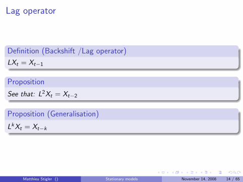
Lag operator

Definition (Backshift /Lag operator)

LXt = Xt−1

Proposition

See that: L2Xt = Xt−2

Proposition (Generalisation)

LkXt = Xt−k


Lag polynomial

We can thus rewrite:

Example (AR(2))

Xt = c + ϕ1Xt−1 + ϕ2Xt−2 + εt

(1− ϕ1L− ϕ2L2)Xt = c + εt

Definition (lag polynomial)

We call lag polynomial: Φ(L) = (1− ϕ1L− ϕ2L2 − . . .− φpLp)

So we write compactly:

Example (AR(2))

Φ(L)Xt = c + εt


Outline

1 Last Lecture



4 Forecasting


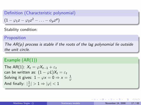
Definition (Characteristic polynomial)

(1− ϕ1z − ϕ2z2 − . . .− φpzp)

Stability condition:

Proposition

The AR(p) process is stable if the roots of the lag polynomial lie outsidethe unit circle.

Example (AR(1))

The AR(1): Xt = ϕXt−1 + εtcan be written as: (1− ϕL)Xt = εtSolving it gives: 1− ϕx = 0⇒ x = 1

ϕ

And finally: | 1ϕ | > 1⇒ |ϕ| < 1


Proof.1 Write an AR(p) as AR(1)

2 Show conditions for the augmented AR(1)

3 Transpose the result to the AR(p)


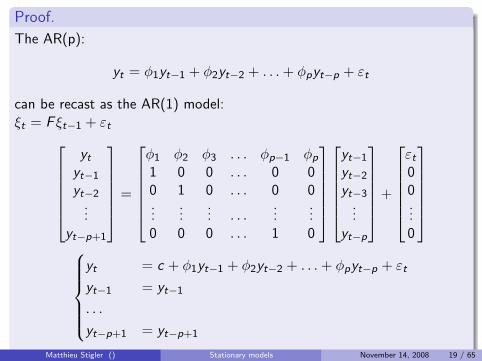
Proof.

The AR(p):

yt = φ1yt−1 + φ2yt−2 + . . .+ φpyt−p + εt

can be recast as the AR(1) model:ξt = F ξt−1 + εt

yt

yt−1

yt−2...

yt−p+1

=

φ1 φ2 φ3 . . . φp−1 φp

1 0 0 . . . 0 00 1 0 . . . 0 0...

...... . . .

......

0 0 0 . . . 1 0

yt−1

yt−2

yt−3...

yt−p

+

εt00...0

yt = c + φ1yt−1 + φ2yt−2 + . . .+ φpyt−p + εt

yt−1 = yt−1

. . .

yt−p+1 = yt−p+1


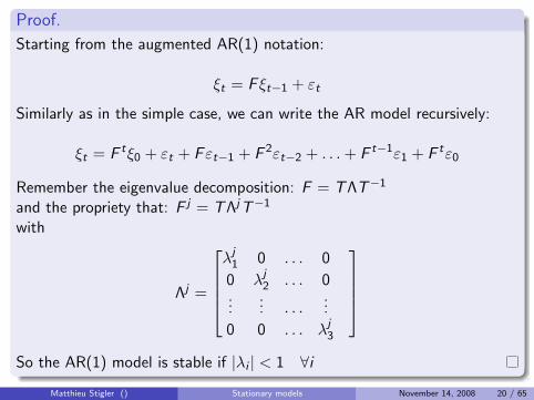
Proof.

Starting from the augmented AR(1) notation:

ξt = F ξt−1 + εt

Similarly as in the simple case, we can write the AR model recursively:

ξt = F tξ0 + εt + Fεt−1 + F 2εt−2 + . . .+ F t−1ε1 + F tε0

Remember the eigenvalue decomposition: F = T ΛT−1

and the propriety that: F j = T ΛjT−1

with

Λj =

λj

1 0 . . . 0

0 λj2 . . . 0

...... . . .

...

0 0 . . . λj3

So the AR(1) model is stable if |λi | < 1 ∀i


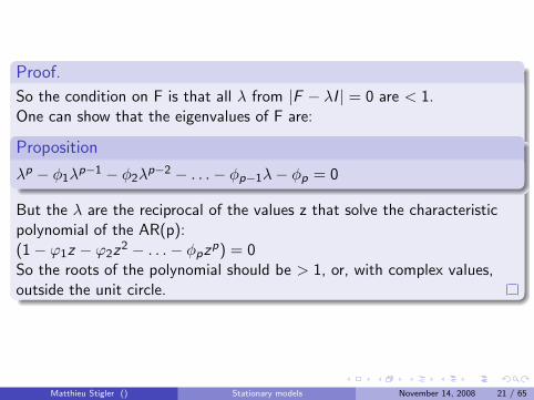
Proof.

So the condition on F is that all λ from |F − λI | = 0 are < 1.One can show that the eigenvalues of F are:

Proposition

λp − φ1λp−1 − φ2λ

p−2 − . . .− φp−1λ− φp = 0

But the λ are the reciprocal of the values z that solve the characteristicpolynomial of the AR(p):(1− ϕ1z − ϕ2z2 − . . .− φpzp) = 0So the roots of the polynomial should be > 1, or, with complex values,outside the unit circle.


Stationarity conditions

The conditions of roots outside the unit circle lead to:

AR(1): |φ| < 1

AR(2):I φ1 + φ2 < 1I φ1 − φ2 < 1I |φ2| < 1


Example

Consider the AR(2) model:

Yt = 0.8Yt−1 + 0.09Yt−2 + εt

Its AR(1) representation is:[yt

yt−1

]=

[0.8 0.091 0

] [yt−1

yt−2

]+

[εt0

]Hence its eigenvalues are taken from:∣∣∣∣0.8− λ 0.09

1 0− λ

∣∣∣∣ = λ2 − 0.8λ− 0.09 = 0

And the eigenvalues are smaller than one:

> Re(polyroot(c(-0.09, -0.8, 1)))

[1] -0.1 0.9


Example

Yt = 0.8Yt−1 + 0.09Yt−2 + εt

Its lag polynomial representation is: (1− 0.8L− 0.09L2)Xt = εtIts characteristic polynomial is hence: (1− 0.8x − 0.09x2) = 0whose solutions lie outside the unit circle:

> Re(polyroot(c(1, -0.8, -0.09)))

[1] 1.111111 -10.000000

And it is the inverse of the previous solutions:

> all.equal(sort(1/Re(polyroot(c(1, -0.8, -0.09)))), Re(polyroot(c(-0.09,

+ -0.8, 1))))

[1] TRUE


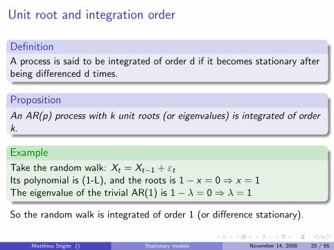
Unit root and integration order

Definition

A process is said to be integrated of order d if it becomes stationary afterbeing differenced d times.

Proposition

An AR(p) process with k unit roots (or eigenvalues) is integrated of orderk.

Example

Take the random walk: Xt = Xt−1 + εtIts polynomial is (1-L), and the roots is 1− x = 0⇒ x = 1The eigenvalue of the trivial AR(1) is 1− λ = 0⇒ λ = 1

So the random walk is integrated of order 1 (or difference stationary).


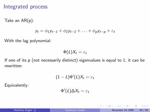
Integrated process

Take an AR(p):

yt = φ1yt−1 + φ2yt−2 + . . .+ φpyt−p + εt

With the lag polynomial:

Φ(L)Xt = εt

If one of its p (not necessarily distinct) eigenvalues is equal to 1, it can berewritten:

(1− L)Φ′(L)Xt = εt

Equivalently:Φ′(L)∆Xt = εt


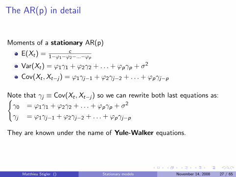
The AR(p) in detail

Moments of a stationary AR(p)

E(Xt) = c1−ϕ1−ϕ2−...−ϕp

Var(Xt) = ϕ1γ1 + ϕ2γ2 + . . .+ ϕpγp + σ2

Cov(Xt ,Xt−j) = ϕ1γj−1 + ϕ2γj−2 + . . .+ ϕpγj−p

Note that γj ≡ Cov(Xt ,Xt−j) so we can rewrite both last equations as:{γ0 = ϕ1γ1 + ϕ2γ2 + . . .+ ϕpγp + σ2

γj = ϕ1γj−1 + ϕ2γj−2 + . . .+ ϕpγj−p

They are known under the name of Yule-Walker equations.


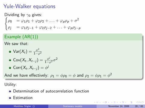
Yule-Walker equations

Dividing by γ0 gives:{ρ0 = ϕ1ρ1 + ϕ2ρ2 + . . .+ ϕpρp + σ2

ρj = ϕ1ρj−1 + ϕ2ρj−2 + . . .+ ϕpρj−p

Example (AR(1))

We saw that:

Var(Xt) = σ2

1−ϕ2

Cov(Xt ,Xt−j) = ϕj

1−ϕ2σ2

Corr(Xt ,Xt−j) = φj

And we have effectively: ρ1 = φρ0 = φ and ρ2 = φρ1 = φ2

Utility:

Determination of autocorrelation function

Estimation


Outline

1 Last Lecture



4 Forecasting


To estimate a AR(p) model from a sample of T we take t=T-p

Methods of moments: estimate sample moments (the γi ), and findparameters (the φ) correspondly

Unconditional ML: assume yp, . . . , y1 ∼ N (0, σ2). Need numericaloptimisation methods.

Conditional Maximum likelihood (=OLS): estimatef (yT , tT−1, . . . , yp+1|yp, . . . , y1; θ) and assume εt ∼ N (0, σ2) andthat yp, . . . , y1 are given

What if errors are not normally distributed? Quasi-maximum likelihoodestimator, is still consistent (in this case) but standard erros need to becorrected.


Outline

1 Last Lecture



4 Forecasting


Moving average models

Two significations!

regression model

Smoothing technique!


MA(1)

Definition (MA(1))

Yt = c + εt + θεt−1

E(Yt) = c

Var(Yt) = (1 + θ2)σ2

Cov(Xt ,Xt−j) =

{θσ2 if j = 1

0 if j > 1

Corr(Xt ,Xt−j) =

{θ

(1+θ2)if j = 1

0 if j > 1

Proposition

A MA(1) is stationnary for every θ


Time

0 20 40 60 80 100

−2

01

2

θθ == 0.5

Time

0 20 40 60 80 100

−4

02

46

8

θθ == 2

Time

0 20 40 60 80 100

−3

−1

12

3

θθ == −0.5

Time

0 20 40 60 80 100

−4

02

46

θθ == −2


2 4 6 8 10

0.0

0.4

0.8

Lag k

ρρ kθθ == 0.5

2 4 6 8 10

0.0

0.4

0.8

Lag k

ρρ k

θθ == 3

2 4 6 8 10

−1.

00.

00.

51.

0

Lag k

ρρ k

θθ == −0.5

2 4 6 8 10

−1.

00.

00.

51.

0

Lag k

ρρ kθθ == −3


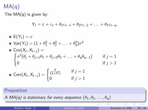
MA(q)

The MA(q) is given by:

Yt = c + εt + θ1εt−1 + θ2εt−2 + . . .+ θ1εt−q

E(Yt) = c

Var(Yt) = (1 + θ21 + θ2

2 + . . .+ θ2q)σ2

Cov(Xt ,Xt−j) ={σ2(θj + θj+1θ1 + θj+2θ2 + . . .+ θqθq−1) if j = 1

0 if j > 1

Corr(Xt ,Xt−j) =

{θ

(1+θ2)if j = 1

0 if j > 1

Proposition

A MA(q) is stationary for every sequence {θ1, θ2, . . . , θq}


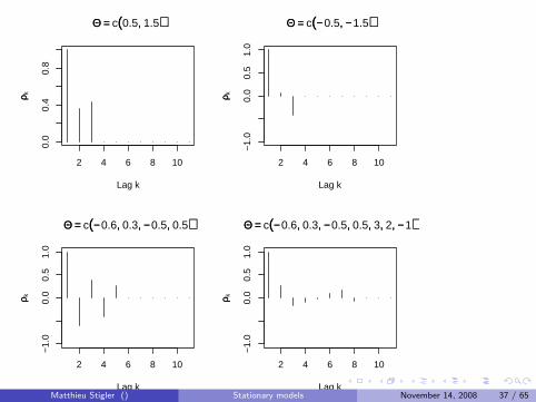
2 4 6 8 10

0.0

0.4

0.8

Lag k

ρρ kΘΘ == c((0.5,, 1.5))

2 4 6 8 10

−1.

00.

00.

51.

0

Lag k

ρρ k

ΘΘ == c((−− 0.5,, −− 1.5))

2 4 6 8 10

−1.

00.

00.

51.

0

Lag k

ρρ k

ΘΘ == c((−− 0.6,, 0.3,, −− 0.5,, 0.5))

2 4 6 8 10

−1.

00.

00.

51.

0

Lag k

ρρ kΘΘ == c((−− 0.6,, 0.3,, −− 0.5,, 0.5,, 3,, 2,, −− 1))


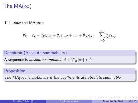
The MA(∞)

Take now the MA(∞):

Yt = εt + θ1εt−1 + θ2εt−2 + . . .+ θ∞ε∞ =∞∑j=0

θjεt−j

Definition (Absolute summability)

A sequence is absolute summable if∑∞

i=0 |αi | < 0

Proposition

The MA(∞) is stationary if the coefficients are absolute summable.


Back to AR(p)

Recall:

Proposition

If the characteristic polynomial of a AR(p) has roots =1, it is notstationary.

See that:(1− φ1yt−1 − φ2yt−2 − . . .− φpyt−p)yt =(1− α1L)(1− α2L) . . . (1− αpL)yt = εtIt has a MA(∞) representation if: α1 6= 1:yt = 1

(1−α1L)(1−α2L)...(1−αpL)εtFurthermore, if the αi (the eigenvalues of the augmented AR(1)) aresmaller than 1, we can write it:

yt =∞∑i=0

βiεt


Estimation of a MA(1)

We do not observe neither εt nor εt−1

But if we know ε0, we know ε1 = Yt − θε0So obtain them recursively and minimize the conditional SSR:S(θ) =

∑Tt=1(yt − εt−1)2

This recquires numerical optimization and works only if |θ| < 1.


Outline

1 Last Lecture



4 Forecasting


ARMA models

The ARMA model is a composite of AR and MA:

Definition (ARMA(p,q))

Xt = c+φ1Xt−1+φ2Xt−2+. . .+φpXt−p+εt−1+θ1εt−1+θ2εt−2+. . .+θεt−q

It can be rewritten properly as:

Φ(L)Yt = c + Θ(L)εt

Theorem

The ARMA(p,q) model is stationary provided the roots of the Φ(L)polynomial lie outside the unit circle.

So only the AR part is involved!


Autocorrelation function of a ARMA(p,q)

Proposition

After q lags, the autocorrelation function follows the pattern of the ARcomponent.

Remember: this is then given by the Yule-Walker equations.


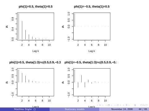
2 4 6 8 10

0.0

0.4

0.8

Lag k

ρρ kphi(1)=0.5, theta(1)=0.5

2 4 6 8 10

−1.

00.

00.

51.

0

Lag k

ρρ k

phi(1)=−0.5, theta(1)=0.5

2 4 6 8 10

−1.

00.

00.

51.

0

Lag k

ρρ k

phi(1)=0.5, theta(1:3)=c(0.5,0.9,−0.3)

2 4 6 8 10

−1.

00.

00.

51.

0

Lag k

ρρ kphi(1)=−0.5, theta(1:3)=c(0.5,0.9,−0.3)


ARIMA(p,d,q)

Now we add a parameter d representing the order of integration (so the Iin ARIMA)

Definition (ARIMA(p,d,q))

ARIMA(p,d,q): Φ(L)∆dYt = Θ(L)εt

Example (Special cases)

White noise: ARIMA(0,0,0) Xt = εt

Random walk : ARIMA(0,1,0): ∆Xt = εt ⇒ Xt = Xt−1 + εt


Estimation and inference

The MLE estimator has to be found numerically.Provided the errors are normaly distributed, the estimator has the usualasymptotical properties:

Consistent

Asymptotically efficients

Normally distributed

If we take into account that the variance had to be estimated, one canrather use the T distribution in small samples.


Outline

1 Last Lecture



4 Forecasting


The Box-Jenkins approach

1 Transform data to achieve stationarity

2 Identify the model, i.e. the parameters of ARMA(p,d,q)

3 Estimation

4 Diagnostic analysis: test residuals


Step 1

Transformations:

Log

Square root

Differenciation

Box-Cox transformation: Y(λ)t

{Y λ

t −1λ for λ 6= 0

log(Y − t) for λ = 0

Is log legitimate?

Process is: yteδt Then zt = log(yt) = δt and remove trend

Process is yt = yt−1 + εt Then (by log(1 + x) ∼= x)∆ log(yt) = yt−yt−1

yt


Step 2

Identification of p,q (d should now be 0 after convenient transformation)Principle of parsimony: prefer small models Recall that

incoporating variables increases fit (R2) but reduces the degrees offreedom and hence precision of estimation and tests.

A AR(1) has a MA(∞) representation

If the MA(q) and AR(p) polynomials have a common root, theARMA(p,q) is similar to ARMA(p-1,q-1).

Usual techniques recquire that the MA polynomial has roots outsidethe unit circle (i.e. is invertible)


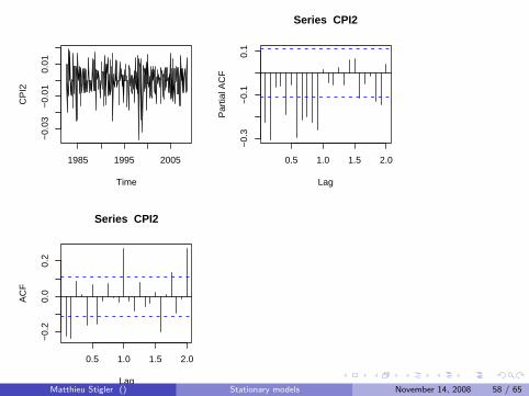
Step 2: identification

How can we determine the parameters p,q?

Look at ACF and PACF with confidence interval

Use information criteriaI Akaike Criterion (AIC)I Schwarz criterion (BIC)

Definition (IC)

AIC (p) = n log σ2 + 2pBIC (p) = n log σ2 + p log n


Step 3: estimation

Estimate the model...R function: arima() argument: order=c(p,d,q)


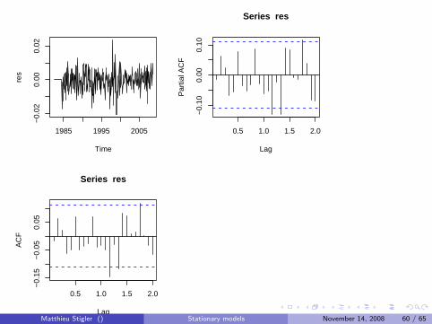
Step 4: diagnostic checks

Test if the residuals are white noise:

1 Autocorrelation

2 Heteroscedasticity

3 Normality


CPI

Time

CP

I

1985 1990 1995 2000 2005

2040

6080

100

120

140


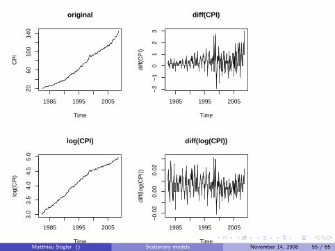
original

Time

CP

I

1985 1995 2005

2060

100

140

diff(CPI)

Time

diff(

CP

I)

1985 1995 2005

−2

−1

01

23

log(CPI)

Time

log(

CP

I)

1985 1995 2005

3.0

3.5

4.0

4.5

5.0

diff(log(CPI))

Time

diff(

log(

CP

I))

1985 1995 2005

−0.

020.

000.

02


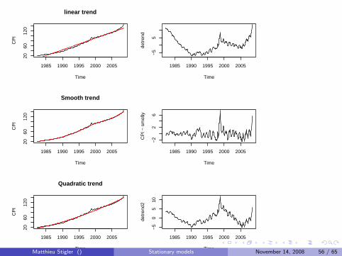
linear trend

Time

CP

I

1985 1990 1995 2000 2005

2060

120

Time

detr

end

1985 1990 1995 2000 2005

−5

5

Smooth trend

Time

CP

I

1985 1990 1995 2000 2005

2060

120

Time

CP

I − s

mo$

y

1985 1990 1995 2000 2005−

22

6

Quadratic trend

Time

CP

I

1985 1990 1995 2000 2005

2060

120

Time

detr

end2

1985 1990 1995 2000 2005

−5

05

10


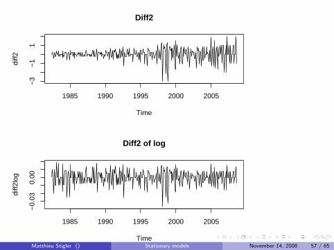
Diff2

Time

diff2

1985 1990 1995 2000 2005

−3

−1

1

Diff2 of log

Time

diff2

log

1985 1990 1995 2000 2005

−0.

030.

00


Time

CP

I2

1985 1995 2005

−0.

03−

0.01

0.01

0.5 1.0 1.5 2.0

−0.

20.

00.

2

Lag

AC

F

Series CPI2

0.5 1.0 1.5 2.0

−0.

3−

0.1

0.1

Lag

Par

tial A

CF

Series CPI2


> library(forecast)

This is forecast 1.17

> fit <- auto.arima(CPI2, start.p = 1, start.q = 1)

> fit

Series: CPI2ARIMA(2,0,1)(2,0,2)[12] with zero mean

Coefficients:ar1 ar2 ma1 sar1 sar2 sma1 sma2

0.2953 -0.2658 -0.9011 0.6021 0.3516 -0.5400 -0.2850s.e. 0.0630 0.0578 0.0304 0.1067 0.1051 0.1286 0.1212

sigma^2 estimated as 4.031e-05: log likelihood = 1146.75AIC = -2277.46 AICc = -2276.99 BIC = -2247.44

> res <- residuals(fit)


Time

res

1985 1995 2005

−0.

020.

000.

02

0.5 1.0 1.5 2.0

−0.

15−

0.05

0.05

Lag

AC

F

Series res

0.5 1.0 1.5 2.0

−0.

100.

000.

10

Lag

Par

tial A

CF

Series res


> Box.test(res)

Box-Pierce test

data: resX-squared = 0.0736, df = 1, p-value = 0.7862


●●●●●●●●●●●●●●●●●●●●●●●●●●

●

●●●

●

●

●

● ●●

●

●

●

●

●●

●

●

●

●

●●

●●●

●●

●

●

●●

●●

●

●●

●●

●●

●

●●

●

●

●

●

●

●●

●

●●

●

●●

● ●

●●

●●

●

●●

●

●● ●

●

●●

●

●

●

●

●●

●●●

●

●

●●

●

●

●●

●

●●●

●●

●

●

●

● ●

●

●

●

●●

●

●

●

●●●

●

●●

●

●● ●●

●

●●

●

●

●

●●●

●

●● ●

●●

●●

●

●

●●

●

●●● ●

●

● ●●

● ● ● ●

●

●

●

●●

●

●

● ●

●

●●●

● ●

●

●●

●

●●

●

● ●

●

●

●●●

●

●●

●

●

●

●●

●●●

●●

● ● ●●

●●●

●●

●

●

●●

●●● ●

●

●●●

●

● ●●

●

●●●

●

●

●●

●

● ●●

● ●●●

●

●

●●

●

●●

●

●

●

●

● ●

●

●

●

●

● ●●

●●

●●

●●

●

●●

●●

●

●

●

●

●

●

●●

●●

●

●

●

●

●

● ●

●

●

●

●

●

−3 −2 −1 0 1 2 3

−0.

020.

01

Normal Q−Q Plot

Theoretical Quantiles

Sam

ple

Qua

ntile

s

−0.02 −0.01 0.00 0.01 0.02

040

80

density.default(x = res)

N = 315 Bandwidth = 0.001481

Den

sity


Outline

1 Last Lecture



4 Forecasting


Notation (Forecast)

yt+j ≡ Et(yt+j) = E(yt+j |yt , yt−1, . . . , εt , εt−1, . . .) is the conditionalexpectation of yt+j given the information available at t.

Definition (J-step-ahead forecast error)

et(j) ≡ yt+j − yt+j

Definition (Mean square prediction error)

MSPE ≡ 1H

∑Hi=1 e2

i


R implementation

To run this file you will need:

R Package forecast

R Package TSA

Data file AjaySeries2.csv put it in a folder called Datasets in the samelevel than your.Rnw file

(Optional) File Sweave.sty which change output style: result is inblue, R commands are smaller. Also in same folder as .Rnw file.


MA, AR and ARMA Matthieu Stigler November 14, 2008...

Documents

Transcript of MA, AR and ARMA Matthieu Stigler November 14, 2008...