MA Advanced Macroeconomics: 6. Solving Models with …karlwhelan.com/MAMacro/part6.pdf · MA...

MA Advanced Macroeconomics:6. Solving Models with Rational Expectations

Karl Whelan

School of Economics, UCD

Spring 2016

Karl Whelan (UCD) Models with Rational Expectations Spring 2016 1 / 36

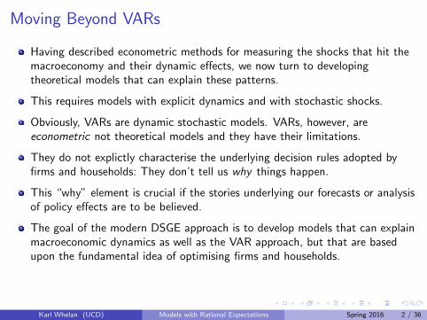
Moving Beyond VARs

Having described econometric methods for measuring the shocks that hit themacroeconomy and their dynamic effects, we now turn to developingtheoretical models that can explain these patterns.

This requires models with explicit dynamics and with stochastic shocks.

Obviously, VARs are dynamic stochastic models. VARs, however, areeconometric not theoretical models and they have their limitations.

They do not explictly characterise the underlying decision rules adopted byfirms and households: They don’t tell us why things happen.

This “why” element is crucial if the stories underlying our forecasts or analysisof policy effects are to be believed.

The goal of the modern DSGE approach is to develop models that can explainmacroeconomic dynamics as well as the VAR approach, but that are basedupon the fundamental idea of optimising firms and households.


Part I

Introduction to Rational Expectations


Introducing Expectations

A key sense in which DSGE models differ from VARs is that while VARs justhave backward-looking dynamics, DSGE models backward-loking andforward-looking dynamics.

The backward-looking dynamics stem, for instance, from identities linkingtoday’s capital stock with last period’s capital stock and this period’sinvestment, i.e. Kt = (1− δ)Kt−1 + It .

The forward-looking dynamics stem from optimising behaviour: What agentsexpect to happen tomorrow is very important for what they decide to dotoday.

Modelling this idea requires an assumption about how people formulateexpectations.

The DSGE approach relies on the idea that people have so-called rationalexpectations.

I will first introduce the idea of rational expectations and describe how tosolve and simulate linear rational expecations models that have both backwardand forward-looking components.


Rational Expectations

Almost all economic transactions rely crucially on the fact that the economy isnot a “one-period game.” Economic decisions have an intertemporal elementto them.

A key issue in macroeconomics is how people formulate expectations aboutthe in the presence of uncertainty.

Prior to the 1970s, this aspect of macro theory was largely ad hoc. Generally,it was assumed that agents used some simple extrapolative rule whereby theexpected future value of a variable was close to some weighted average of itsrecent past values.

This approach criticised in the 1970s by economists such as Robert Lucas andThomas Sargent. Lucas and Sargent instead promoted the use of analternative approach which they called “rational expectations.”

In economics, rational expectations usually means two things:

1 They use publicly available information in an efficient manner. Thus,they do not make systematic mistakes when formulating expectations.

2 They understand the structure of the model economy and base theirexpectations of variables on this knowledge.


Rational Expectations as a Baseline

Rational expectations is clearly a strong assumption.

The structure of the economy is complex and in truth nobody truly knowshow everything works.

But one reason for using rational expectations as a baseline assumption is thatonce one has specified a particular model of the economy, any otherassumption about expectations means that people are making systematicerrors, which seems inconsistent with rationality.

Still, behavioural economists have now found lots of examples of deviationsfrom rationality in people’s economic behaviour.

But rational expectations requires one to be explicit about the full limitationsof people’s knowledge and exactly what kind of mistakes they make. Andwhile rational expectations is a clear baseline, once one moves away from itthere are lots of essentially ad hoc potential alternatives.

At least at present, the profession has no clear agreed alternative to rationalexpectations as a baseline assumption.

And like all models, rational expectations models need to be assessed on thebasis of their ability to fit the data.


Part II

Single Stochastic Difference Equations


First-Order Stochastic Difference Equations

Lots of models in economics take the form

yt = xt + aEtyt+1

The equation just says that y today is determined by x and by tomorrow’sexpected value of y . But what determines this expected value? Rationalexpectations implies a very specific answer.

Under rational expectations, the agents in the economy understand theequation and formulate their expectation in a way that is consistent with it:

Etyt+1 = Etxt+1 + aEtEt+1yt+2

This last term can be simplified to

Etyt+1 = Etxt+1 + aEtyt+2

because EtEt+1yt+2 = Etyt+2.

This is known as the Law of Iterated Expectations: It is not rational for me toexpect to have a different expectation next period for yt+2 than the one that Ihave today.


Repeated Substitution

Substituting this into the previous equation, we get

yt = xt + aEtxt+1 + a2Etyt+2

Repeating this by substituting for Etyt+2, and then Etyt+3 and so on gives

yt = xt + aEtxt+1 + a2Etxt+2 + ....+ aN−1Etxt+N−1 + aNEtyt+N

Which can be written in more compact form as

yt =N−1∑k=0

akEtxt+k + aNEtyt+N

Usually, it is assumed that

limN→∞

aNEtyt+N = 0

So the solution is

yt =∞∑k=0

akEtxt+k

This solution underlies the logic of a very large amount of modernmacroeconomics.


Example: Asset Pricing

Consider an asset that can be purchased today for price Pt and which yields adividend of Dt . Suppose there is a close alternative to this asset that will yielda guaranteed rate of return of r .

Then, for a risk neutral investor will only hold the asset if it yields the samerate of return, i.e. if

Dt + EtPt+1

Pt= 1 + r

This can be re-arranged to give

Pt =Dt

1 + r+

EtPt+1

1 + r

The repeated substitution solution is

Pt =∞∑k=0

(1

1 + r

)k+1

EtDt+k

This equation, which states that asset prices should equal a discountedpresent-value sum of expected future dividends, is usually known as thedividend-discount model.


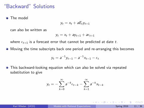
“Backward” Solutions

The modelyt = xt + aEtyt+1

can also be written asyt = xt + ayt+1 + aεt+1

where εt+1 is a forecast error that cannot be predicted at date t.

Moving the time subscripts back one period and re-arranging this becomes

yt = a−1yt−1 − a−1xt−1 − εt

This backward-looking equation which can also be solved via repeatedsubstitution to give

yt = −∞∑k=0

a−kεt−k −∞∑k=1

a−kxt−k


Choosing Between Forward and Backward Solutions

The forward and backward solutions are both correct solutions to thefirst-order stochastic difference equation (as are all linear combinations ofthem). Which solution we choose to work with depends on the value of theparameter a.

If |a| > 1, then the weights on future values of xt in the forward solution willexplode. In this case, it is most likely that the forward solution will notconverge to a finite sum. Even if it does, the idea that today’s value of ytdepends more on values of xt far in the distant future than it does on today’svalues is not one that we would be comfortable with. In this case, practicalapplications should focus on the backwards solution.

However, the equation holds for any set of shocks εt such that Et−1εt = 0. Sothe solution is indeterminate: We can’t actually predict what will happen withyt even if we know the full path for xt .

But if |a| < 1 then the weights in the backwards solution are explosive and theforward solution is the one to focus on. Also, this solution is determinate.Knowing the path of xt will tell you the path of yt .


Rational Bubbles

In most cases, it is assumed that |a| < 1.

In this case, the assumption that

limN→∞

aNEtyt+N = 0

amounts to a statement that yt can’t grow too fast.

What if it doesn’t hold? Then the solution can have other elements.

Let

y∗t =∞∑k=0

akEtxt+k

And let yt = y∗t + bt be any other solution. The solution must satisfy

y∗t + bt = xt + aEty∗t+1 + aEtbt+1

By construction, one can show that y∗t = xt + aEty∗t+1.


Rational Bubbles, Continued

This means the additional component satisfies

bt = aEtbt+1

Because |a| < 1, this means b is always expected to get bigger in absolutevalue, going to infinity in expectation. This is a bubble.

Note that the term bubbles is usually associated with irrational behaviour byinvestors. But, in this model, the agents have rational expectations. This is arational bubble.

There may be restrictions in the real economy that stop b growing forever.But constant growth is not the only way to satisfy bt = aEtbt+1. Thefollowing process also works:

bt+1 =

(aq)−1 bt + et+1 with probability qet+1 with probability 1− q

where Etet+1 = 0.

This is a bubble that everyone knows is going to crash eventually. And eventhen, a new bubble can get going. Imposing limN→∞ aNEtyt+N = 0 rules outbubbles of this (or any other) form.


From Structural to Reduced Form Relationships

The solution

yt =∞∑k=0

akEtxt+k

provides useful insights into how the variable yt is determined.

However, without some assumptions about how xt evolves over time, itcannot be used to give precise predictions about they dynamics of yt .

Ideally, we want to be able to simulate the behaviour of yt on the computer.

One reason there is a strong linkage between DSGE modelling and VARs isthat this question is usually addressed by assuming that the exogenous“driving variables” such as xt are generated by backward-looking time seriesmodels like VARs.

Consider for instance the case where the process driving xt is

xt = ρxt−1 + εt

where |ρ| < 1.


From Structural to Reduced Form Relationships, Continued

In this case, we haveEtxt+k = ρkxt

Now the model’s solution can be written as

yt =

[ ∞∑k=0

(aρ)k]xt

Because |aρ| < 1, the infinite sum converges to∞∑k=0

(aρ)k =1

1− aρ

Remember this identity from the famous Keynesian multiplier formula.

So, in this case, the model solution is

yt =1

1− aρxt

Macroeconomists call this a reduced-form solution for the model: Togetherwith the equation descrining the evolution of xt , it can easily be simulated ona computer.


The DSGE Recipe

While this example is obviously a relatively simple one, it illustrates thegeneral principal for getting predictions from DSGE models:

1 Obtain structural equations involving expectations of future drivingvariables, (in this case the Etxt+k terms).

2 Make assumptions about the time series process for the driving variables(in this case xt)

3 Solve for a reduced-form solution than can be simulated on thecomputer along with the driving variables.

Finally, note that the reduced-form of this model also has a VAR-likerepresentation, which can be shown as follows:

yt =1

1− aρ(ρxt−1 + εt)

= ρyt−1 +1

1− aρεt

So both the xt and yt series have purely backward-looking representations.Even this simple model helps to explain how theoretical models tend topredict that the data can be described well using a VAR.


Another Example: The Permanent Income Hypothesis

Consider, for example, a simple “permanent income” model in whichconsumption depends on a present discounted value of after-tax income

ct = γ

∞∑k=0

βkEtyt+k

Suppose that income has followed the process

yt = (1 + g) yt−1 + εt

In this case, we haveEtyt+k = (1 + g)k yt

So the reduced-form representation is

ct = γ

[ ∞∑k=0

(β (1 + g))k]yt

Assuming that β (1 + g) < 1, this becomes

ct =γ

1− β (1 + g)yt


The Lucas Critique

Think about this example. The structural equation

ct = γ

∞∑k=0

βkEtyt+k

is always true for this model

But the reduced-form representation

ct =γ

1− β (1 + g)yt

depends on the process for yt taking a particular form. Should that processchange, the reduced-form process will change.

In a famous 1976 paper, Robert Lucas pointed out that the assumption ofrational expectations implied that the coefficients in reduced-form modelswould change if expectations about the future changed.

Lucas stressed that this could make reduced-form econometric models basedon historical data useless for policy analysis. This problem is now known asthe Lucas critique of econometric models.


An Example: Temporary Tax Cuts

Suppose the government is thinking about a temporary one-period income taxcut. Consider yt to be after-tax labour income, so it would be temporarilyboosted by the tax cut.

They ask their economic advisers for an estimate of the effect on consumptionof the tax cut. The advisers run a regression of consumption on after-taxincome.

If, in the past, consumers had generally expected income growth of g , thenthese regressions will produce a coefficient of approximately γ

1−β(1+g) on

income. So, the advisers conclude that for each €1 of income produced bythe tax cut, there will be an increase in consumption of € γ

1−β(1+g) .

But if the households have rational expectations, then then each €1 of taxcut will produce only €γ of extra consumption.

Suppose β = 0.95 and g = 0.02. In this case, the advisor concludes that eachunit of tax cuts is worth extra 32γ (= γ

1−β(1+g) ) in consumption. In reality, the

tax cut will produce only γ units of extra consumption. Being off by a factorof 32 constitutes a big mistake in assessing the effect of this policy.


The Lucas Critique and the Limitations of VAR Analysis

The tax cut example gets the logic of the critique across but perhaps not itsgenerality.

Today’s DSGE models feature policy equations that describe how monetarypolicy is set via rules relating interest rates to inflation and unemployment;how fiscal variables depends on other macro variables; what the exchange rateregime is.

These models all feature rational expectations, so changes to these policyrules will be expected to alter the reduced-form VAR-like structures associatedwith these economies.

This is an important “selling point” for modern DSGE models. These modelscan explain why VARs fit the data well, but they can be considered superiortools for policy analysis.

They explain how reduced-form VAR-like equations are generated by theprocesses underlying policy and other driving variables. However, while VARmodels do not allow reduced-form correlations change over time, a fullyspecified DSGE model can explain such patterns as the result of structuralchanges in policy rules.


Second-Order Stochastic Difference Equations

Variables that are characterized by

yt =∞∑k=0

akEtxt+k

are jump variables. They only depends on what’s happening today and what’sexpected to happen tomorrow. If expectations about the future change, theywill jump. Nothing that happened in the past will restrict their movement.

This may be an ok characterization of financial variables like stock prices butit’s harder to argue with it as a description of variables in the real economylike employment, consumption or investment.

Many models in macroeconomics feature variables which depend on both theexpected future values and their past values. They are characterized bysecond-order difference equations of the form

yt = ayt−1 + bEtyt+1 + xt


Solving Second-Order Stochastic Difference Equations

Here’s one way of solving second-order SDEs. Suppose there was a value λsuch that

vt = yt − λyt−1followed a first-order stochastic difference equation of the form

vt = αEtvt+1 + βxt

We’d know how to solve that for vt and then back out the values for yt .

From the fact that yt = vt + λyt−1, we can re-write the original equation as

vt + λyt−1 = ayt−1 + b (Etvt+1 + λyt) + xt

= ayt−1 + bEtvt+1 + bλ (vt + λyt−1) + xt

This re-arranges to give

(1− bλ)vt = bEtvt+1 + xt +(bλ2 − λ+ a

)yt−1


Solving Second-Order Stochastic Difference Equations

By definition, λ was a number such that the vt it defined followed a first-orderstochastic difference equation. This means that λ satisfies:

bλ2 − λ+ a = 0

This is a quadratic equation, so there are two values of λ that satisfy it. Foreither of these values, we can characterize vt by

vt =b

1− bλEtvt+1 +

1

1− bλxt

=1

1− bλ

∞∑k=0

(b

1− bλ

)k

Etxt+k

And yt obeys

yt = λyt−1 +1

1− bλ

∞∑k=0

(b

1− bλ

)k

Etxt+k

Usually, only one of the potential values of λ is less than one in absolutevalue, so this delivers the unique stable solution.


Example: A Hybrid New Keynesian Phillips Curve

Last term, we introduced the so-called New Keynesian Phillips curve

πt = βEtπt+1 + νxt ,

where xt is a measure of inflationary pressures.

Many empirical studies have suggested that this formulation has difficulty inexplaining the persistence observed in the inflation data.

Some have proposed a “hybrid” variant:

πt = γf Etπt+1 + γbπt−1 + κxt

with the lagged element coming from some fraction of the population beingnon-rational price-setters who rely on past inflation for their current behaviour.

The solution for this model takes the form

πt = λπt−1 +κ

1− γf λ

∞∑k=0

(γf

1− γf λ

)k

Etxt+k

where λ is a solution toγf λ

2 − λ+ γb = 0


Example: A Hybrid New Keynesian Phillips Curve

In general, there will be two possible values of λ to solve the so-calledcharacteristic equation of the model. Usually, only one of these values willwork as the λ in this formulation.

Consider the case where the model is

πt = θEtπt+1 + (1− θ)πt−1 + κxt

In this case, the possible solutions of the characteristic equation are λ1 = 1and λ2 = 1−θ

θ .

If 0 < θ ≤ 0.5, then the stable solution is

πt = πt−1 +κ

1− θ

∞∑k=0

(θ

1− θ

)k

Etxt+k

Alternatively if 0.5 ≤ θ < 1, then the stable solution is

πt =

(1− θθ

)πt−1 +

κ

θ

∞∑k=0

Etxt+k


Part III

Systems of Stochastic Difference Equations


Systems of Rational Expectations Equations

So far, we have only looked at a single equation linking two variables.However, it turns out that the logic of the first-order stochastic differenceequation underlies the solution methodology for just about all rationalexpectations models.

Suppose one has a vector of variables

Zt =

z1tz2t.znt

It turns out that a lot of macroeconomic models can be represented by anequation of the form

Zt = BEtZt+1 + Xt

where B is an n × n matrix. The logic of repeated substitution can also beapplied to this model, to give a solution of the form

Zt =∞∑k=0

BkEtXt+k


Eigenvalues

As with the single-equation model, this will only give a stable non-explosivesolution under certain conditions.

A value λi is an eigenvalue of the matrix B if there exists a vector ei (knownas an eigenvector) such that

Bei = λiei

Many n × n matrices have n distinct eigenvalues. Denote by P the matrixthat has as its columns n eigenvectors corresponding to these eigenvalues. Inthis case,

BP = PΩ

where

Ω =

λ1 0 0 00 λ2 0 00 0 00 0 0 λn

is a diagonal matrix of eigenvalues.


Stability Condition

Note now that this equation implies that

B = PΩP−1

This tells us something about the relationship between eigenvalues and higherpowers of B because

Bn = PΩnP−1 = P

λn1 0 0 00 λn2 0 00 0 00 0 0 λnn

P−1

So, the difference between lower and higher powers of B is that the higherpowers depend on the eigenvalues taken to the power of n. If all of theeigenvalues are inside the unit circle (i.e. less than one in absolute value) thenall of the entries in Bn will tend towards zero as n→∞.

So, a condition that ensures that a model of the form Zt = BEtZt+1 + Xt hasa unique stable forward-looking solution is that the eigenvalues of B are allinside the unit circle.


How Are Eigenvalues Calculated

Consider, for example, a 2× 2 matrix.

A =

(a11 a12a21 a22

)Suppose A has two eigenvalues, λ1 and λ2 and define λ as the vector

λ =

(λ1λ2

)The fact that there are eigenvectors which when multiplied by A− λI equal avector of zeros means that the determinant of the matrix

A− λI =

(a11 − λ1 a12

a21 a22 − λ2

)equals zero.

So solving the quadratic formula

(a11 − λ1a12) (a22 − λ2)− a12a21 = 0

gives the two eigenvalues of A.


More General Models: The Binder-Pesaran Method

Consider a vector Zt characterized by

Zt = AZt−1 + BEtZt+1 + HXt

The restriction to one-lag one-lead form is only apparent, and the companionmatrix trick can be used to allow this model to represent models with n leadsand lags. In this sense, this equation summarizes all possible linear rationalexpectations models.

Binder and Pesaran (1996) solved this model in a manner exactly analagousto the second-order difference equation discussed earlier. Find a matrix Csuch that Wt = Zt − CZt−1 obeys a first-order matrix equation of the form

Wt = FEtWt+1 + GXt

In other words, we transform the problem of solving the “second-order”system in equation into a simpler first-order system.


More General Models: The Binder-Pesaran Method

What must the matrix C be? Using the fact that

Zt = Wt + CZt−1

The model can be re-written as

Wt + CZt−1 = AZt−1 + B (EtWt+1 + CZt) + HXt

= AZt−1 + B (EtWt+1 + C (Wt + CZt−1)) + HXt

This re-arranges to

(I − BC )Wt = BEtWt+1 +(BC 2 − C + A

)Zt−1 + HXt

Because C is the matrix that such that Wt follows a first-orderforward-looking matrix equation (with no extra Zt−1 terms) it follows that

BC 2 − C + A = 0

This “matrix quadratic equation” can be solved to give C . Solving theseequations is non-trivial (see paper on the website). One method uses the factthat C = BC 2 + A, to solve for it iteratively as follows. Provide an initialguess, say C0 = I , and then iterate on Cn = BC 2

n−1 + A until all the entries inCn converge.


Model Solution

Once we know C , we have

Wt = FEtWt+1 + GXt

where

F = (I − BC )−1 B

G = (I − BC )−1 H

Assuming the all the eigenvalues of F are inside the unit circle, this has astable forward-looking solution

Wt =∞∑k=0

F kEt (GXt+k)

which can be written in terms of the original equation as

Zt = CZt−1 +∞∑k=0

F kEt (GXt+k)


Reduced-Form Representation

Suppose we assume that the driving variables Xt follow a VAR representationof the form

Xt = DXt−1 + εt

where D has eigenvalues inside the unit circle.

This implies EtXt+k = DkXt , so the model solution is

Zt = CZt−1 +

[ ∞∑k=0

F kGDk

]Xt

The infinite sum in this equation will converge to a matrix P, so the modelhas a reduced-form representation

Zt = CZt−1 + PXt

which can be simulated along with the VAR process for the driving variables.

This provides a relatively simple recipe for simulating DSGE models: Specifythe A, B and H matrices; solve for C , F and G ; specify a VAR process for thedriving variables; and then obtain the reduced-form representations.


General Formulation

The equations we get from models will often contain multiple values ofdifferent variables at time t.

This isn’t a problem. We can plug the model into a computer program as

KZt = AZt−1 + BEtZt+1 + HXt

Then the program can multiply both sides by K−1 to give

Zt = K−1AZt−1 + K−1BEtZt+1 + K−1HXt

Which is a format that can be solved using the Binder-Pesaran method.

All of this seems a bit complicated. In practice, it’s not so hard. You figureout what your model implies in terms of the K , A, B and H matrices (most ofthe entries are usually zero). Then the computer gives you representation ofthe form

Zt = CZt−1 + PXt

Xt = DXt−1 + εt

which you can start to do calculations with.


MA Advanced Macroeconomics: 6. Solving Models with …karlwhelan.com/MAMacro/part6.pdf · MA...

Documents

Transcript of MA Advanced Macroeconomics: 6. Solving Models with …karlwhelan.com/MAMacro/part6.pdf · MA...