MA 554: Homework 1
59
MA 554: Homework 1 Yingwei Wang ∗ Department of Mathematics, Purdue University, West Lafayette, IN, USA 1 The induction of Japanese empire succession Theorem 1.1. Let S = ∞ i=1 S i , where means disjoint union. Suppose the cardinality ¯ ¯ S i < ∞, ∀i. Let f i : S i → S i−1 , ∀i =2, 3, ··· . If ¯ ¯ S i > 0, ∀i, then ∃a i ∈ S i such that f i (a i )= a i−1 . Proof. 1. Step I. Consider the image of S 2 in S 1 under the map f 2 : f 2 : S 2 → f 2 (S 2 ) ⊂ S 1 . Choose a 1 ∈ f 2 (S 2 ) and a 2 ∈ f −1 2 (a 1 ) ∈ S 2 . 2. Step II. Consider the image of S 3 in S 2 under the map f 3 : f 3 : S 3 → f 3 (S 3 ) ⊂ S 2 . If a 2 ∈ f 3 (S 3 ), then it is fine. We can choose a 3 ∈ S 3 such that a 3 ∈ f −1 3 (a 2 ). If not, we have to choose another a ′ 1 ∈ f 2 (S 2 ) and a ′ 2 ∈ f −1 2 (a ′ 1 ) ∈ S 2 in Step I. Since 0 < ¯ ¯ S i < ∞, ∀i, we can always find proper a 1 and a 2 such that a 2 ∈ f 3 (S 3 ). Keep doing the Step I and Step II, we can get a sequence {a i } ∞ i=1 such that f i (a i )= a i−1 , where a i ∈ S i . * E-mail address : [email protected]; Tel : 765 237 7149 1
-
Upload
nguyenquynh -
Category
Documents
-
view
233 -
download
1
Transcript of MA 554: Homework 1
MA 554: Homework 1
Yingwei Wang ∗
Department of Mathematics, Purdue University, West Lafayette, IN, USA
1 The induction of Japanese empire succession
Theorem 1.1. Let S =∐
∞
i=1 Si, where∐
means disjoint union. Suppose the cardinality¯Si < ∞, ∀i. Let
fi : Si → Si−1, ∀i = 2, 3, · · · .
If ¯Si > 0, ∀i, then ∃ai ∈ Si such that fi(ai) = ai−1.
Proof. 1. Step I.
Consider the image of S2 in S1 under the map f2:
f2 : S2 → f2(S2) ⊂ S1.
Choose a1 ∈ f2(S2) and a2 ∈ f−12 (a1) ∈ S2.
2. Step II.
Consider the image of S3 in S2 under the map f3:
f3 : S3 → f3(S3) ⊂ S2.
If a2 ∈ f3(S3), then it is fine. We can choose a3 ∈ S3 such that a3 ∈ f−13 (a2).
If not, we have to choose another a′1 ∈ f2(S2) and a′2 ∈ f−12 (a′1) ∈ S2 in Step I. Since
0 < ¯Si < ∞, ∀i, we can always find proper a1 and a2 such that a2 ∈ f3(S3).Keep doing the Step I and Step II, we can get a sequence {ai}
∞
i=1 such that
fi(ai) = ai−1,
where ai ∈ Si.
∗E-mail address : [email protected]; Tel : 765 237 7149
1
Yingwei Wang Linear Algebra
2 Notherian Ring
Definition 2.1. Let R be a ring. If every ideal can be generated by finitely many elements,
then say R is notherian.
Theorem 2.1. If R is noethrian, then every element r ∈ R can be written as
r = Πni=1qi,
where q′is are irreducible.
Proof. First, claim that in the Definition 2.1, “finitely generated”⇔ “ascending chaincondition”.
(⇐) : For any ideal I ⊂ R, let us choose a1 ∈ I such that (a1) ⊂ I; If (a1) 6= I, thenchoose a2 ∈ I \ (a1); If (a1, a2) & I, then we can choose a3 ∈ I \ (a1, a2). Keep dong this,we can get an ascending chain:
(a1) ⊂ (a1, a2) ⊂ (a1, a2, a3) ⊂ · · · ⊂ I.
This chain should satisfy the “ascending chain condition”. Thus, there exists j such that
(a1, a2, · · · , aj) = (a1, a2, · · · , aj, aj+1) = · · · = I.
It follows that I is finitely generated.(⇒) : Consider any ascending chain
I1 & I2 & · · · Ii & Ii+1 · · ·
Suppose
I1 = (a1, · · · , ak1),
I2 = (a1, · · · , ak1, · · · , ak2),
· · ·
Ii = (a1, · · · , ak1, · · · , ak2, · · · , aki),
· · · .
Since for ∀i, Ii is finitely generated, there exists j such that
Ij = Ij+1 = · · · .
It follows that R satisfy the “ascending chain condition”.Second, let us prove this theorem.Let r ∈ R, a 6= 0. If r is irreducible, then we are done.If r is reducible, then r = r1r2, where r1 and r2 are non-unit. If both r1, r2 are
irreducible, then we are done. If not, let us suppose r2 is reducible, then we have r2 = r3r4.
2
Yingwei Wang Linear Algebra
Keep doing this, by Theorem 1.1, we can get a sequence {r2k}∞
k=1, such that
· · · r2k | r2(k−1) | · · · r4 | r2 | r.
Now we have an ascending chain
(r) ⊂ (r2) ⊂ (r4) · · · .
Since R is notherian, then there exists j such that
(r2j) = (r2(j+1)) = · · · .
It implies that r2j is irreducible.Besides, if r1 is reducible at the beginning, then we can also get an ascending chain,
and get the same conclusion.It follows that finally, r can be written as
r = Πni=1qi,
where q′is are irreducible.
3
MA 554: Homework 2
Yingwei Wang ∗
Department of Mathematics, Purdue University, West Lafayette, IN, USA
1 The Chinese Remainder Theorem
Lemma 1.1. Suppose q1, q2, · · · , qn be pairwise coprime positive integers, i.e.
(qi, qj) = 1, ∀i 6= j, i, j = 1, 2, · · · , n.
Let
di =∏
j 6=i
qj.
Then
(d1, d2, · · · , dn) = 1. (1.1)
Proof. First, claim that
(di, qi) = 1, ∀i = 1, 2, · · · , n. (1.2)
Without loss of generality, assume there exists a prime p1 such that
(d1, q1) = p1 6= 1.
Then on one hand,
p1 | d1 = q2q3 · · · qn,
⇒ p1 | qk, for some k = 2, 3, · · ·n. (1.3)
∗E-mail address : [email protected]; Tel : 765 237 7149
1
Yingwei Wang Linear Algebra
On the other hand,p1 | q1. (1.4)
By Eqs.(1.3)-(1.4), we can get
(p1, pk) = p1 6= 1,
which contradicts with the fact that p1 and pk are coprime.Now we have proved that (1.2) is true.Second, claim that (1.1) is true.Assume there exists a prime p such that
(d1, d2, · · · , dn) = p 6= 1.
Then we havep | di, ∀i = 1, 2, · · · , n. (1.5)
In addition, by (1.2), we have
p ∤ qi, ∀i = 1, 2, · · · , n. (1.6)
It is obvious that (1.5) contradicts with (1.6) by the definition of di and the factthat p is a prime hence irreducible.
2 RSA algorithm
The keys for the RSA algorithm are generated the following way:
1. Choose two distinct large prime numbers p and q;
2. Compute n = pq;
3. Compute ϕ(n) = (p− 1)(q − 1), where ϕ(n) is Euler’s totient function;
4. Choose an integer e such that 1 < e < ϕ(n) and greatest common denominatorof (e, ϕ(n)) = 1, i.e. e and ϕ(n) are coprime;
5. Determine de = 1 mod ϕ(n), i.e. d is the multiplicative inverse of e mod ϕ(n).
How to use the RSA algorithm?
2
Yingwei Wang Linear Algebra
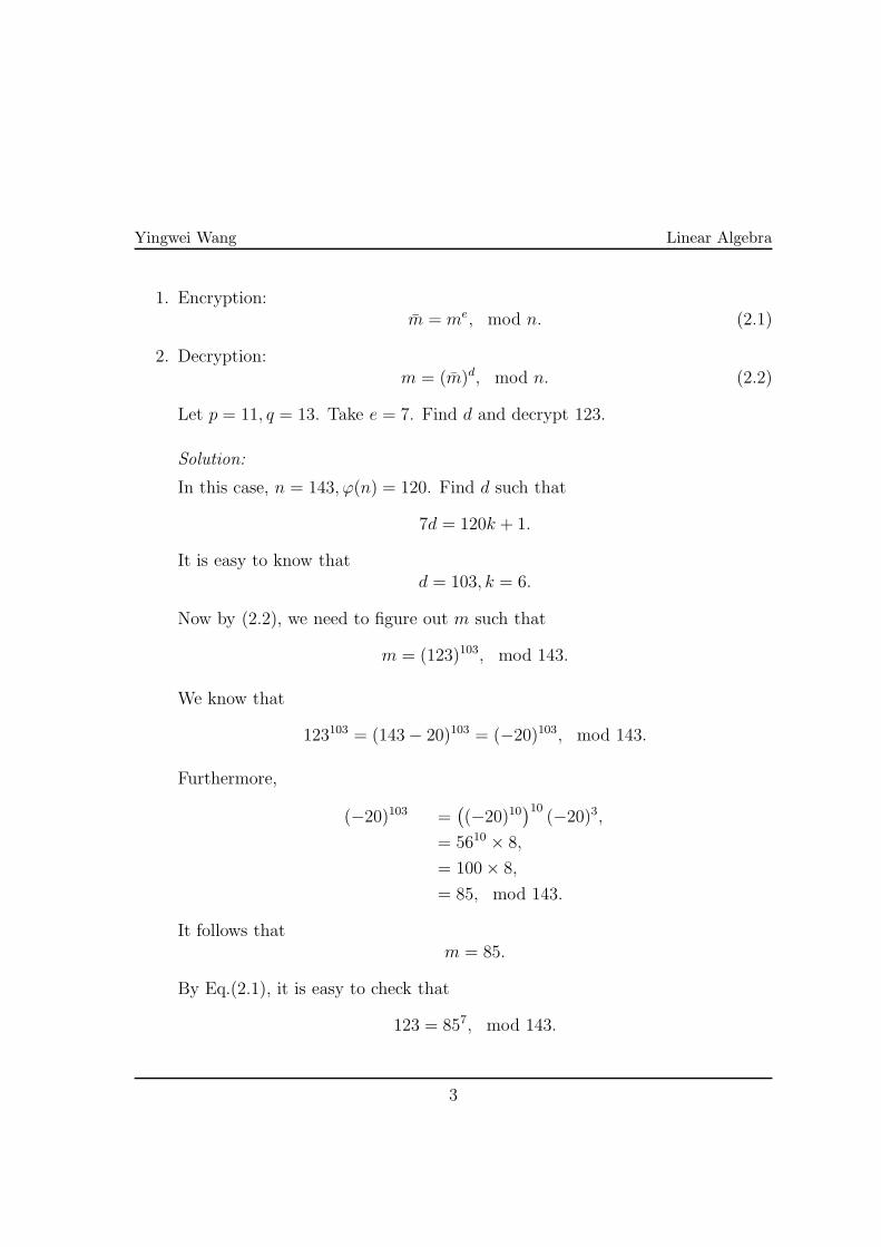
1. Encryption:m = me, mod n. (2.1)
2. Decryption:m = (m)d, mod n. (2.2)
Let p = 11, q = 13. Take e = 7. Find d and decrypt 123.
Solution:
In this case, n = 143, ϕ(n) = 120. Find d such that
7d = 120k + 1.
It is easy to know thatd = 103, k = 6.
Now by (2.2), we need to figure out m such that
m = (123)103, mod 143.
We know that
123103 = (143− 20)103 = (−20)103, mod 143.
Furthermore,
(−20)103 =(
(−20)10)10
(−20)3,
= 5610 × 8,
= 100× 8,
= 85, mod 143.
It follows thatm = 85.
By Eq.(2.1), it is easy to check that
123 = 857, mod 143.
3
MA 554: Homework 3
Yingwei Wang ∗
Department of Mathematics, Purdue University, West Lafayette, IN, USA
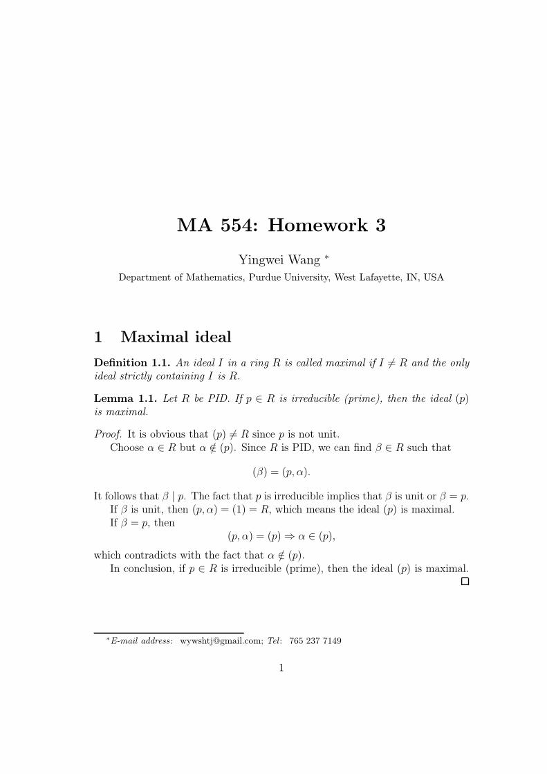
1 Maximal ideal
Definition 1.1. An ideal I in a ring R is called maximal if I 6= R and the onlyideal strictly containing I is R.
Lemma 1.1. Let R be PID. If p ∈ R is irreducible (prime), then the ideal (p)is maximal.
Proof. It is obvious that (p) 6= R since p is not unit.Choose α ∈ R but α /∈ (p). Since R is PID, we can find β ∈ R such that
(β) = (p, α).
It follows that β | p. The fact that p is irreducible implies that β is unit or β = p.If β is unit, then (p, α) = (1) = R, which means the ideal (p) is maximal.If β = p, then
(p, α) = (p) ⇒ α ∈ (p),
which contradicts with the fact that α /∈ (p).In conclusion, if p ∈ R is irreducible (prime), then the ideal (p) is maximal.
∗E-mail address : [email protected]; Tel : 765 237 7149
1
Yingwei Wang Linear Algebra
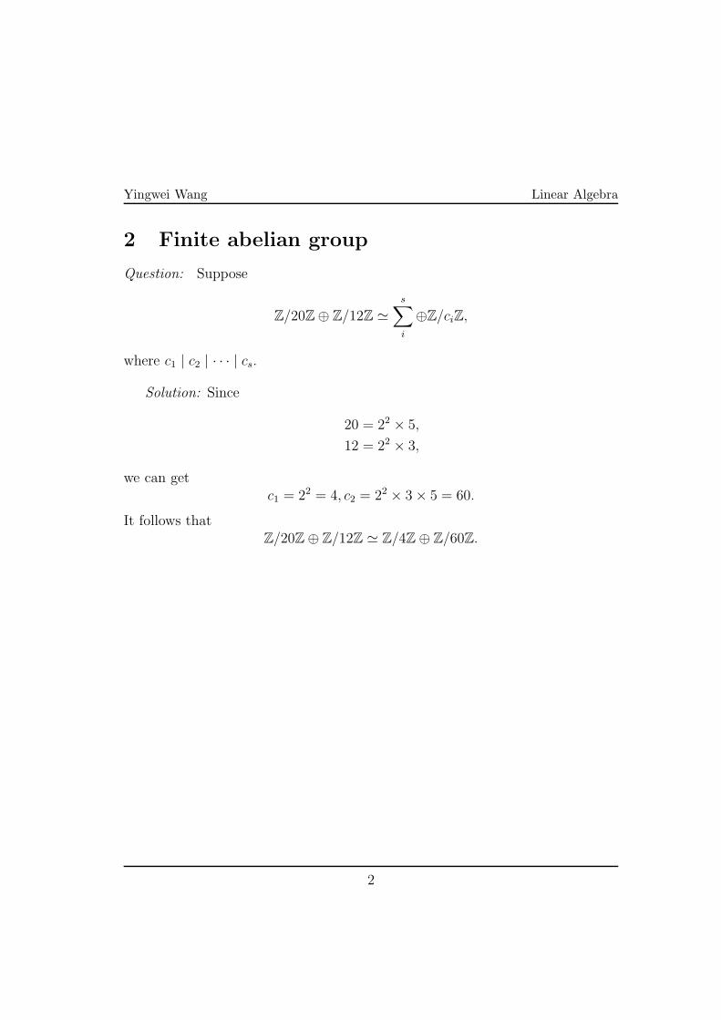
2 Finite abelian group
Question: Suppose
Z/20Z⊕ Z/12Z ≃s∑
i
⊕Z/ciZ,
where c1 | c2 | · · · | cs.
Solution: Since
20 = 22 × 5,
12 = 22 × 3,
we can getc1 = 22 = 4, c2 = 22 × 3× 5 = 60.
It follows thatZ/20Z⊕ Z/12Z ≃ Z/4Z⊕ Z/60Z.
2
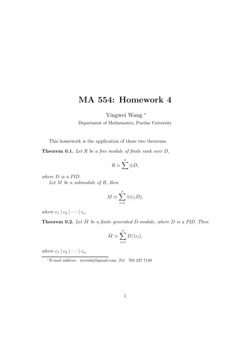
MA 554: Homework 4
Yingwei Wang ∗
Department of Mathematics, Purdue University
This homework is the application of these two theorems.
Theorem 0.1. Let R be a free module of finite rank over D,
R ≃
n∑
⊕D,
where D is a PID.
Let M be a submodule of R, then
M ≃
s∑
i=1
⊕(ciD),
where c1 | c2 | · · · | cs.
Theorem 0.2. Let M be a finite generated D-module, where D is a PID. Then
M ≃n
∑
i=1
D/(ci),
where c1 | c2 | · · · | cn.
∗E-mail address : [email protected]; Tel : 765 237 7149
1
Yingwei Wang Linear Algebra
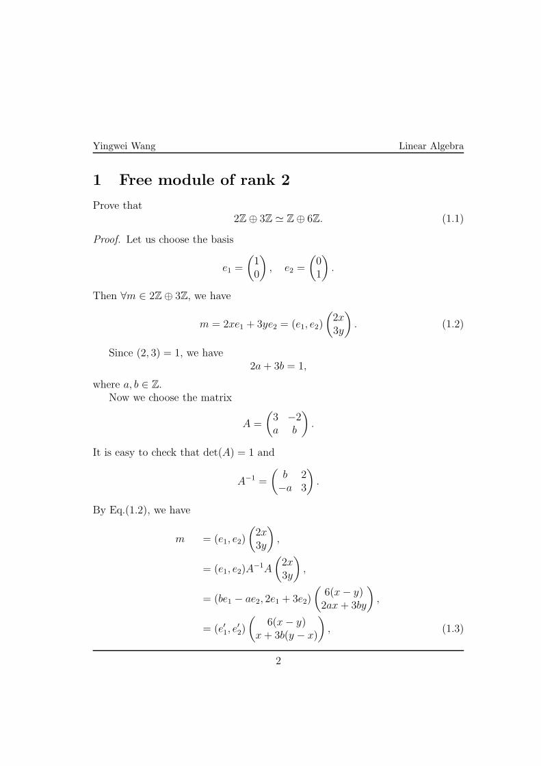
1 Free module of rank 2
Prove that2Z⊕ 3Z ≃ Z⊕ 6Z. (1.1)
Proof. Let us choose the basis
e1 =
(
10
)
, e2 =
(
01
)
.
Then ∀m ∈ 2Z⊕ 3Z, we have
m = 2xe1 + 3ye2 = (e1, e2)
(
2x3y
)
. (1.2)
Since (2, 3) = 1, we have2a+ 3b = 1,
where a, b ∈ Z.Now we choose the matrix
A =
(
3 −2a b
)
.
It is easy to check that det(A) = 1 and
A−1 =
(
b 2−a 3
)
.
By Eq.(1.2), we have
m = (e1, e2)
(
2x3y
)
,
= (e1, e2)A−1A
(
2x3y
)
,
= (be1 − ae2, 2e1 + 3e2)
(
6(x− y)2ax+ 3by
)
,
= (e′1, e′
2)
(
6(x− y)x+ 3b(y − x)
)
, (1.3)
2
Yingwei Wang Linear Algebra
where
e′1= be1 − ae2,
e′2= 2e1 + 3e2.
Since 6(x − y) ∈ 6Z, x + 3b(y − x) ∈ Z, we know that under the new basis{e′
1, e′
2}, the element m can be written in the form (1.3). It follows that m ∈
Z⊕ 6Z.Similarly, it also can be shown that if n ∈ Z⊕ 6Z, then n ∈ 2Z⊕ 3Z.In conclusion, we can get Eq.(1.1)
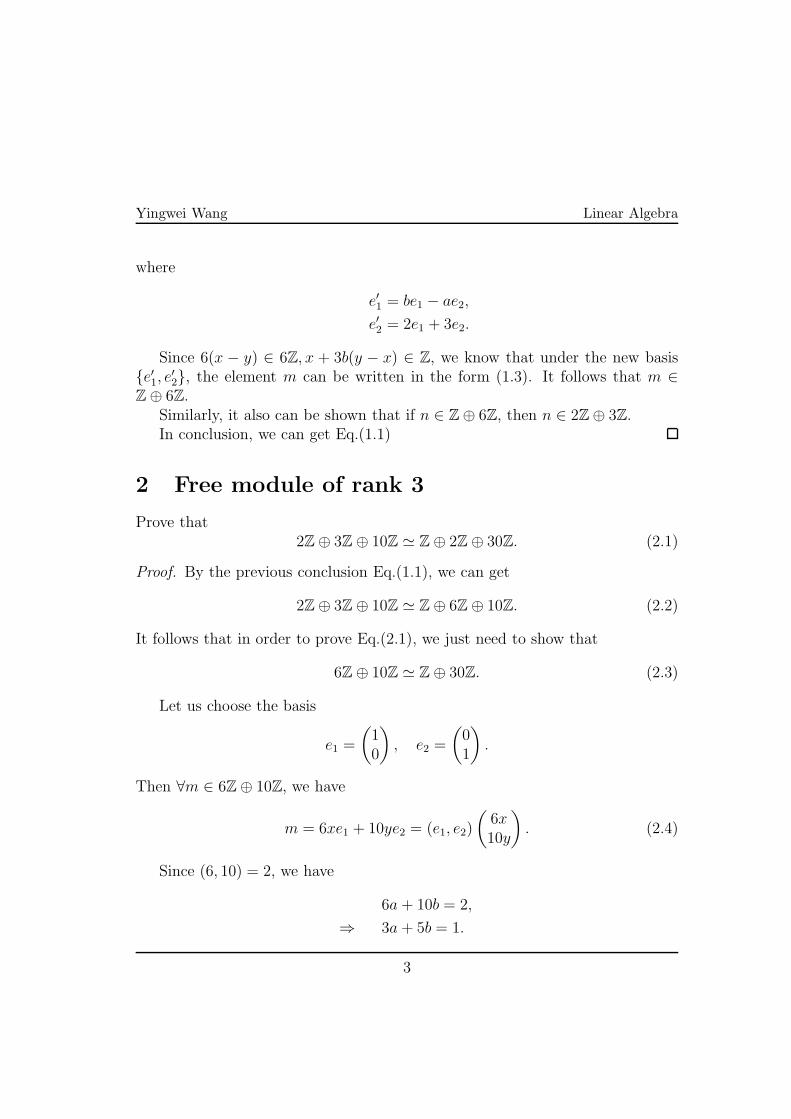
2 Free module of rank 3
Prove that2Z⊕ 3Z⊕ 10Z ≃ Z⊕ 2Z⊕ 30Z. (2.1)
Proof. By the previous conclusion Eq.(1.1), we can get
2Z⊕ 3Z⊕ 10Z ≃ Z⊕ 6Z⊕ 10Z. (2.2)
It follows that in order to prove Eq.(2.1), we just need to show that
6Z⊕ 10Z ≃ Z⊕ 30Z. (2.3)
Let us choose the basis
e1 =
(
10
)
, e2 =
(
01
)
.
Then ∀m ∈ 6Z⊕ 10Z, we have
m = 6xe1 + 10ye2 = (e1, e2)
(
6x10y
)
. (2.4)
Since (6, 10) = 2, we have
6a + 10b = 2,
⇒ 3a + 5b = 1.
3
Yingwei Wang Linear Algebra
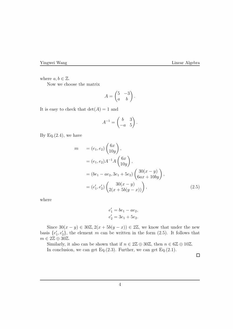
where a, b ∈ Z.Now we choose the matrix
A =
(
5 −3a b
)
.
It is easy to check that det(A) = 1 and
A−1 =
(
b 3−a 5
)
.
By Eq.(2.4), we have
m = (e1, e2)
(
6x10y
)
,
= (e1, e2)A−1A
(
6x10y
)
,
= (be1 − ae2, 3e1 + 5e2)
(
30(x− y)6ax+ 10by
)
,
= (e′1, e′
2)
(
30(x− y)2(x+ 5b(y − x))
)
, (2.5)
where
e′1= be1 − ae2,
e′2= 3e1 + 5e2.
Since 30(x − y) ∈ 30Z, 2(x + 5b(y − x)) ∈ 2Z, we know that under the newbasis {e′
1, e′
2}, the element m can be written in the form (2.5). It follows that
m ∈ 2Z⊕ 30Z.Similarly, it also can be shown that if n ∈ 2Z⊕ 30Z, then n ∈ 6Z⊕ 10Z.In conclusion, we can get Eq.(2.3). Further, we can get Eq.(2.1).
4
Yingwei Wang Linear Algebra
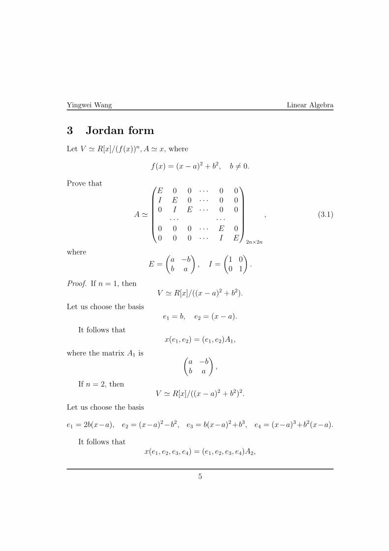
3 Jordan form
Let V ≃ R[x]/(f(x))n, A ≃ x, where
f(x) = (x− a)2 + b2, b 6= 0.
Prove that
A ≃
E 0 0 · · · 0 0I E 0 · · · 0 00 I E · · · 0 0
· · · · · ·0 0 0 · · · E 00 0 0 · · · I E
2n×2n
, (3.1)
where
E =
(
a −bb a
)
, I =
(
1 00 1
)
.
Proof. If n = 1, thenV ≃ R[x]/((x− a)2 + b2).
Let us choose the basise1 = b, e2 = (x− a).
It follows thatx(e1, e2) = (e1, e2)A1,
where the matrix A1 is(
a −bb a
)
,
If n = 2, thenV ≃ R[x]/((x− a)2 + b2)2.
Let us choose the basis
e1 = 2b(x−a), e2 = (x−a)2−b2, e3 = b(x−a)2+b3, e4 = (x−a)3+b2(x−a).
It follows thatx(e1, e2, e3, e4) = (e1, e2, e3, e4)A2,
5
Yingwei Wang Linear Algebra
where the matrix A2 is(
E 0I E
)
.
By induction, for n ∈ N, A should be in the form (3.1).
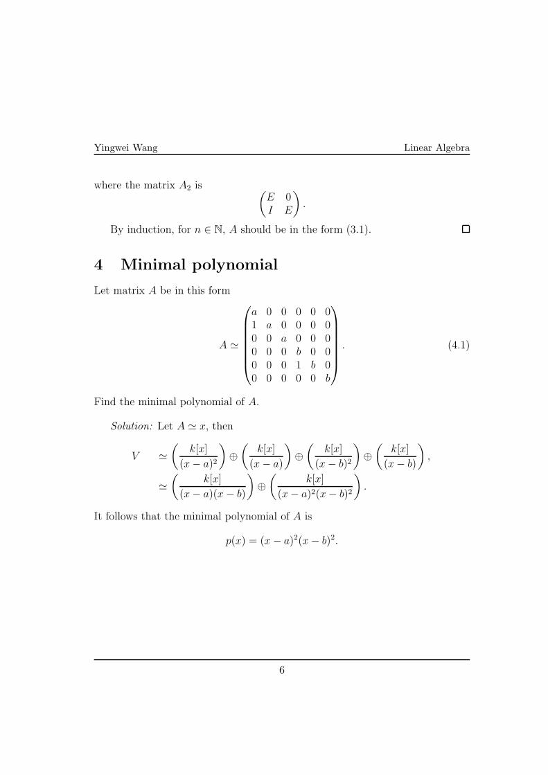
4 Minimal polynomial
Let matrix A be in this form
A ≃
a 0 0 0 0 01 a 0 0 0 00 0 a 0 0 00 0 0 b 0 00 0 0 1 b 00 0 0 0 0 b
. (4.1)
Find the minimal polynomial of A.
Solution: Let A ≃ x, then
V ≃
(
k[x]
(x− a)2
)
⊕
(
k[x]
(x− a)
)
⊕
(
k[x]
(x− b)2
)
⊕
(
k[x]
(x− b)
)
,
≃
(
k[x]
(x− a)(x− b)
)
⊕
(
k[x]
(x− a)2(x− b)2
)
.
It follows that the minimal polynomial of A is
p(x) = (x− a)2(x− b)2.
6
MA 554: Homework 5
Yingwei Wang ∗
Department of Mathematics, Purdue University
1 Reflection
Definition 1.1. A matrix A is said to be a reflection matrix iff
AAT = ATA = I, (1.1)
det(A) = −1. (1.2)
Theorem 1.1. Let A be a 3 × 3 reflection matrix. Then −1 is one of the
eigenvalues.
Proof. Consider the characteristic polynomial
χA(λ) = det(A− λI),
= −λ3 + a2λ2 + a1λ+ det(A),
= −λ3 + a2λ2 + a1λ− 1. (1.3)
On one hand, it is easy to know that χA(0) = −1 and χA(−∞) = ∞, whichimplies that χA(λ) = 0 must have at least one root in (−∞, 0).
On the other hand, due to the property Eq.(1.1), all of the eigenvalues of Ashould satisfy
|λ| = 1 ⇒ λ = ±1.
Now it is clear that λ = −1 must be one of the eigenvalues of A.
∗E-mail address : [email protected]; Tel : 765 237 7149
1

Yingwei Wang Linear Algebra
2 Characteristic polynomial
Let a, b and c be elements of a field F , and let A be the following 3 × 3 matrixover F :
A =
0 0 c
1 0 b
0 1 a
. (2.1)
Show that the characteristic polynomial for A is
x3 − ax2 − bx− c, (2.2)
and that this is also the minimal polynomial for A.
Proof. It is easy to know that
det(λI −A) =
λ 0 −c
−1 λ −b
0 −1 λ− a
= (λ− a)λ2 + b(−λ)− c,
= λ3 − aλ2 − bλ− c.
It follows that the characteristic polynomial for A is Eq.(2.2).Besides, it is easy to know that
A2 =
0 c ac
0 b c+ ab
1 a b+ a2
. (2.3)
Suppose there exist a polynomial of degree 2
p(x) = dx2 + ex+ f (2.4)
such that p(A) = 0.Assume the 3× 3 matrix B = (bij) = p(A), then
b11 = 0 ⇒ f = 0,
b31 = 0 ⇒ d+ f = 0 ⇒ d = 0,
b21 = 0 ⇒ e+ f = 0 ⇒ e = 0.
2
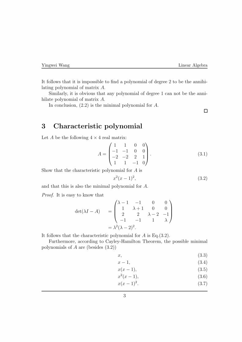
Yingwei Wang Linear Algebra
It follows that it is impossible to find a polynomial of degree 2 to be the annihi-lating polynomial of matrix A.
Similarly, it is obvious that any polynomial of degree 1 can not be the anni-hilate polynomial of matrix A.
In conclusion, (2.2) is the minimal polynomial for A.
3 Characteristic polynomial
Let A be the following 4× 4 real matrix:
A =
1 1 0 0−1 −1 0 0−2 −2 2 11 1 −1 0
. (3.1)
Show that the characteristic polynomial for A is
x2(x− 1)2, (3.2)
and that this is also the minimal polynomial for A.
Proof. It is easy to know that
det(λI − A) =
λ− 1 −1 0 01 λ+ 1 0 02 2 λ− 2 −1−1 −1 1 λ
= λ2(λ− 2)2.
It follows that the characteristic polynomial for A is Eq.(3.2).Furthermore, according to Cayley-Hamilton Theorem, the possible minimal
polynomials of A are (besides (3.2))
x, (3.3)
x− 1, (3.4)
x(x− 1), (3.5)
x2(x− 1), (3.6)
x(x− 1)2. (3.7)
3
Yingwei Wang Linear Algebra
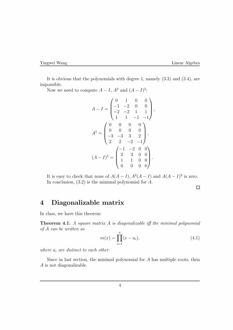
It is obvious that the polynomials with degree 1, namely (3.3) and (3.4), areimpossible.
Now we need to compute A− I, A2 and (A− I)2:
A− I =
0 1 0 0−1 −2 0 0−2 −2 1 11 1 −1 −1
,
A2 =
0 0 0 00 0 0 0−3 −3 3 22 2 −2 −1
,
(A− I)2 =
−1 −2 0 02 3 0 01 1 0 00 0 0 0
.
It is easy to check that none of A(A− I), A2(A− I) and A(A− I)2 is zero.In conclusion, (3.2) is the minimal polynomial for A.
4 Diagonalizable matrix
In class, we have this theorem:
Theorem 4.1. A square matrix A is diagonalizable iff the minimal polynomial
of A can be written as
m(x) =
n∏
i=1
(x− ai), (4.1)
where ai are distinct to each other.
Since in last section, the minimal polynomial for A has multiple roots, thenA is not diagonalizable.
4
Yingwei Wang Linear Algebra
5 Nilpotent matrix
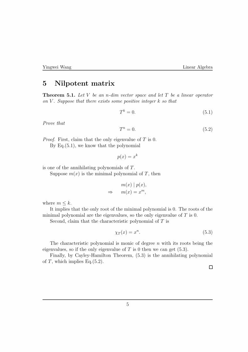
Theorem 5.1. Let V be an n-dim vector space and let T be a linear operator
on V . Suppose that there exists some positive integer k so that
T k = 0. (5.1)
Prove that
T n = 0. (5.2)
Proof. First, claim that the only eigenvalue of T is 0.By Eq.(5.1), we know that the polynomial
p(x) = xk
is one of the annihilating polynomials of T .Suppose m(x) is the minimal polynomial of T , then
m(x) | p(x),
⇒ m(x) = xm,
where m ≤ k.It implies that the only root of the minimal polynomial is 0. The roots of the
minimal polynomial are the eigenvalues, so the only eigenvalue of T is 0.Second, claim that the characteristic polynomial of T is
χT (x) = xn. (5.3)
The characteristic polynomial is monic of degree n with its roots being theeigenvalues, so if the only eigenvalue of T is 0 then we can get (5.3).
Finally, by Cayley-Hamilton Theorem, (5.3) is the annihilating polynomialof T , which implies Eq.(5.2).
5
MA 554: Homework 6
Yingwei Wang ∗
Department of Mathematics, Purdue University
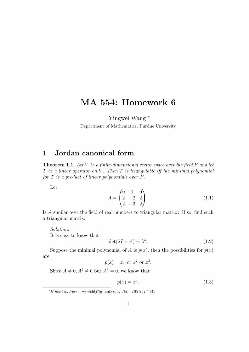
1 Jordan canonical form
Theorem 1.1. Let V be a finite-dimensional vector space over the field F and let
T be a linear operator on V . Then T is triangulable iff the minimal polynomial
for T is a product of linear polynomials over F .
Let
A =
0 1 02 −2 22 −3 2
. (1.1)
Is A similar over the field of real numbers to triangular matrix? If so, find sucha triangular matrix.
Solution:
It is easy to know thatdet(λI − A) = λ3. (1.2)
Suppose the minimal polynomial of A is p(x), then the possibilities for p(x)are
p(x) = x, or x2 or x3.
Since A 6= 0, A2 6= 0 but A3 = 0, we know that
p(x) = x3. (1.3)
∗E-mail address : [email protected]; Tel : 765 237 7149
1
Yingwei Wang Linear Algebra
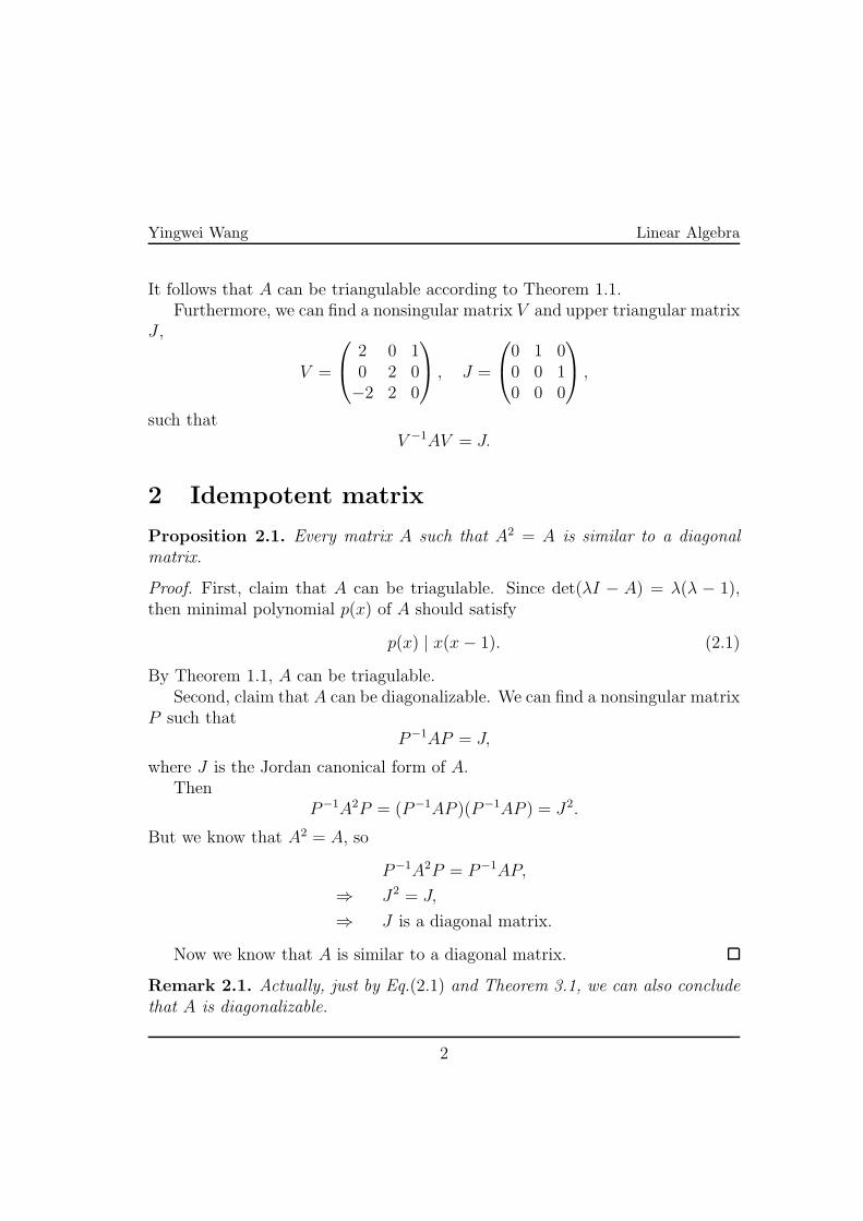
It follows that A can be triangulable according to Theorem 1.1.Furthermore, we can find a nonsingular matrix V and upper triangular matrix
J ,
V =
2 0 10 2 0−2 2 0
, J =
0 1 00 0 10 0 0
,
such thatV −1AV = J.
2 Idempotent matrix
Proposition 2.1. Every matrix A such that A2 = A is similar to a diagonal
matrix.
Proof. First, claim that A can be triagulable. Since det(λI − A) = λ(λ − 1),then minimal polynomial p(x) of A should satisfy
p(x) | x(x− 1). (2.1)
By Theorem 1.1, A can be triagulable.Second, claim that A can be diagonalizable. We can find a nonsingular matrix
P such thatP−1AP = J,
where J is the Jordan canonical form of A.Then
P−1A2P = (P−1AP )(P−1AP ) = J2.
But we know that A2 = A, so
P−1A2P = P−1AP,
⇒ J2 = J,
⇒ J is a diagonal matrix.
Now we know that A is similar to a diagonal matrix.
Remark 2.1. Actually, just by Eq.(2.1) and Theorem 3.1, we can also conclude
that A is diagonalizable.
2
Yingwei Wang Linear Algebra
3 Diagonalizable matrix
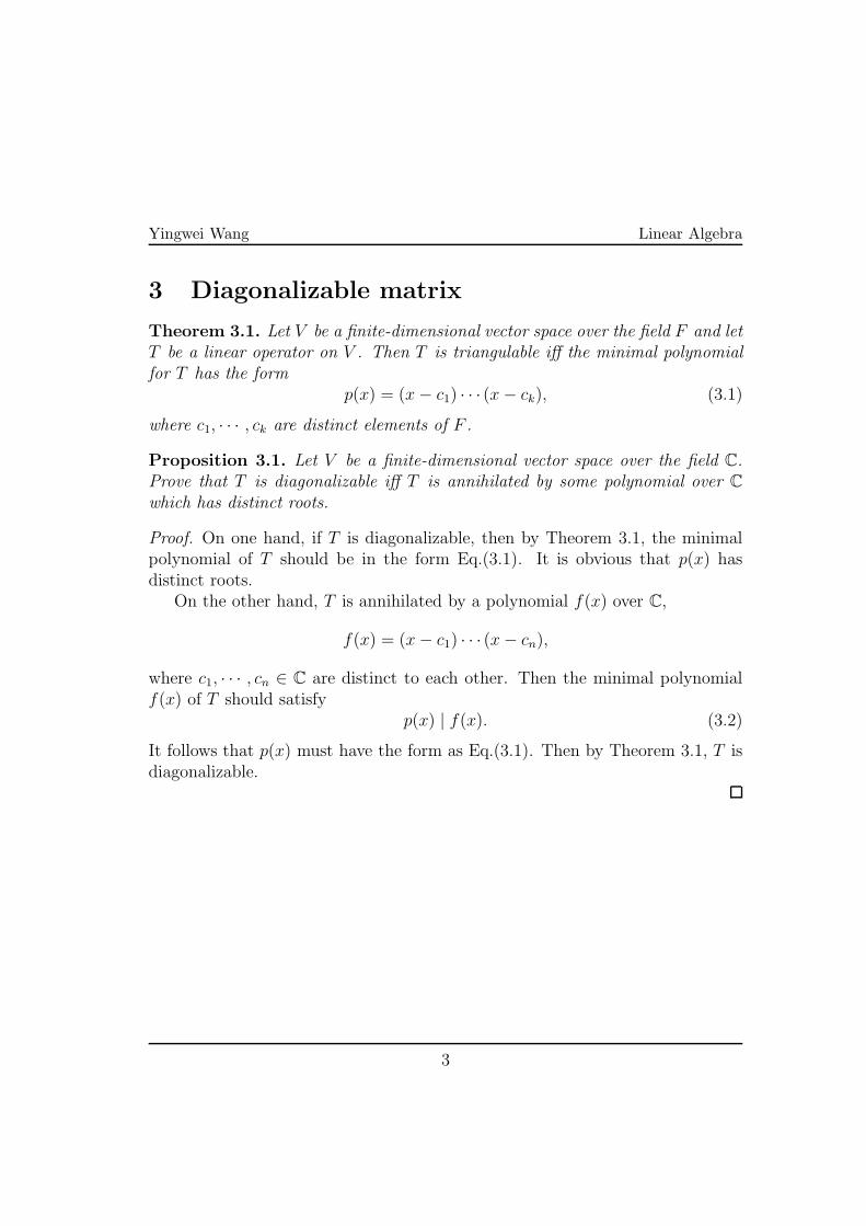
Theorem 3.1. Let V be a finite-dimensional vector space over the field F and let
T be a linear operator on V . Then T is triangulable iff the minimal polynomial
for T has the form
p(x) = (x− c1) · · · (x− ck), (3.1)
where c1, · · · , ck are distinct elements of F .
Proposition 3.1. Let V be a finite-dimensional vector space over the field C.
Prove that T is diagonalizable iff T is annihilated by some polynomial over C
which has distinct roots.
Proof. On one hand, if T is diagonalizable, then by Theorem 3.1, the minimalpolynomial of T should be in the form Eq.(3.1). It is obvious that p(x) hasdistinct roots.
On the other hand, T is annihilated by a polynomial f(x) over C,
f(x) = (x− c1) · · · (x− cn),
where c1, · · · , cn ∈ C are distinct to each other. Then the minimal polynomialf(x) of T should satisfy
p(x) | f(x). (3.2)
It follows that p(x) must have the form as Eq.(3.1). Then by Theorem 3.1, T isdiagonalizable.
3
Yingwei Wang Linear Algebra
4 3 dimensional matrix
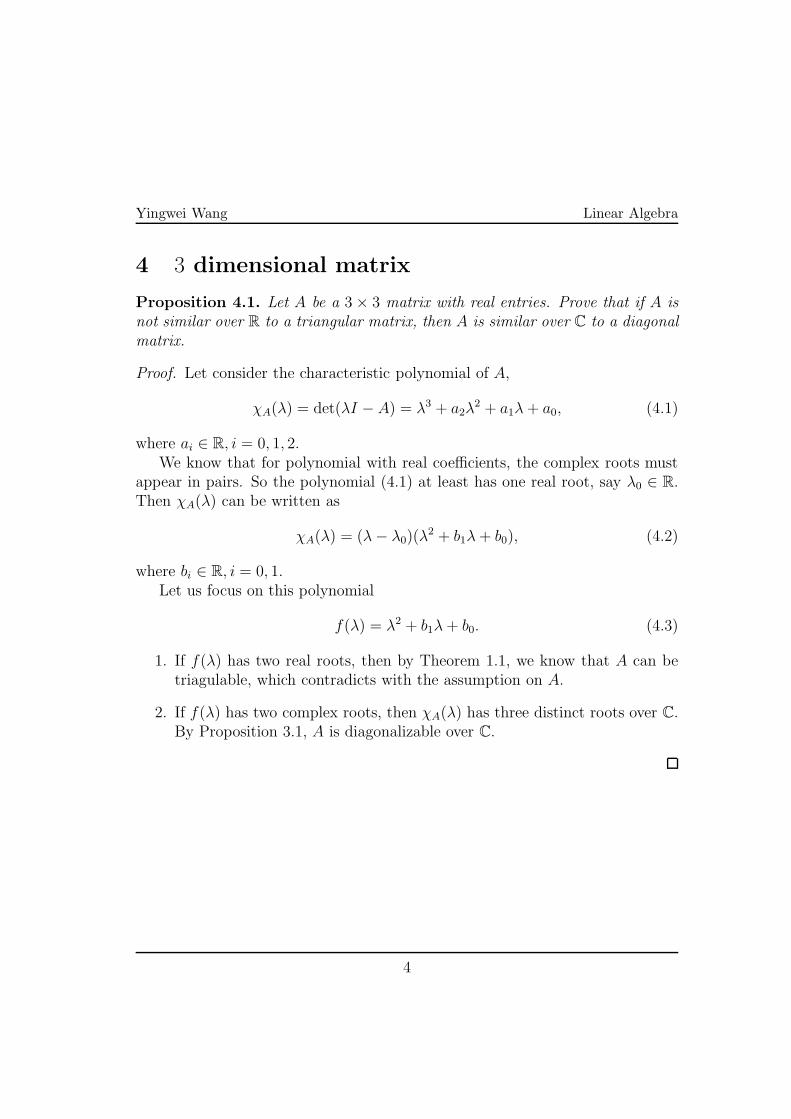
Proposition 4.1. Let A be a 3 × 3 matrix with real entries. Prove that if A is
not similar over R to a triangular matrix, then A is similar over C to a diagonal
matrix.
Proof. Let consider the characteristic polynomial of A,
χA(λ) = det(λI − A) = λ3 + a2λ2 + a1λ+ a0, (4.1)
where ai ∈ R, i = 0, 1, 2.We know that for polynomial with real coefficients, the complex roots must
appear in pairs. So the polynomial (4.1) at least has one real root, say λ0 ∈ R.Then χA(λ) can be written as
χA(λ) = (λ− λ0)(λ2 + b1λ+ b0), (4.2)
where bi ∈ R, i = 0, 1.Let us focus on this polynomial
f(λ) = λ2 + b1λ+ b0. (4.3)
1. If f(λ) has two real roots, then by Theorem 1.1, we know that A can betriagulable, which contradicts with the assumption on A.
2. If f(λ) has two complex roots, then χA(λ) has three distinct roots over C.By Proposition 3.1, A is diagonalizable over C.
4
MA 554: Homework 7
Yingwei Wang ∗
Department of Mathematics, Purdue University
1 Powers of triangular matrices
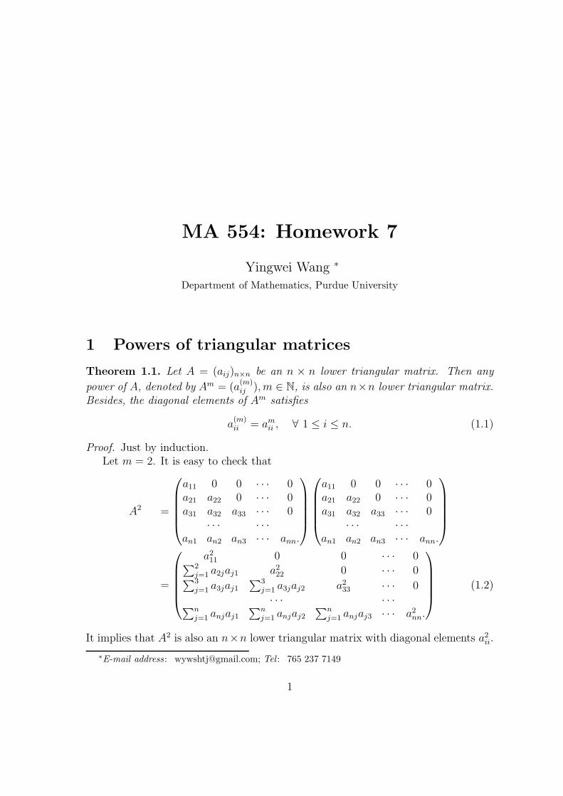
Theorem 1.1. Let A = (aij)n×n be an n × n lower triangular matrix. Then any
power of A, denoted by Am = (a(m)ij ), m ∈ N, is also an n×n lower triangular matrix.
Besides, the diagonal elements of Am satisfies
a(m)ii = amii , ∀ 1 ≤ i ≤ n. (1.1)
Proof. Just by induction.Let m = 2. It is easy to check that
A2 =
a11 0 0 · · · 0a21 a22 0 · · · 0a31 a32 a33 · · · 0
· · · · · ·
an1 an2 an3 · · · ann.
a11 0 0 · · · 0a21 a22 0 · · · 0a31 a32 a33 · · · 0
· · · · · ·
an1 an2 an3 · · · ann.
=
a211 0 0 · · · 0∑2
j=1 a2jaj1 a222 0 · · · 0∑3
j=1 a3jaj1∑3
j=1 a3jaj2 a233 · · · 0
· · · · · ·∑n
j=1 anjaj1∑n
j=1 anjaj2∑n
j=1 anjaj3 · · · a2nn.
(1.2)
It implies that A2 is also an n×n lower triangular matrix with diagonal elements a2ii.
∗E-mail address : [email protected]; Tel : 765 237 7149
1
Yingwei Wang Linear Algebra
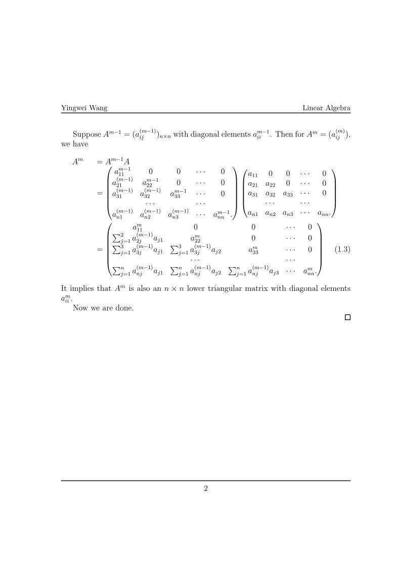
Suppose Am−1 = (a(m−1)ij )n×n with diagonal elements am−1
ii . Then for Am = (a(m)ij ),
we have
Am = Am−1A
=
am−111 0 0 · · · 0
a(m−1)21 am−1
22 0 · · · 0
a(m−1)31 a
(m−1)32 am−1
33 · · · 0· · · · · ·
a(m−1)n1 a
(m−1)n2 a
(m−1)n3 · · · am−1
nn .
a11 0 0 · · · 0a21 a22 0 · · · 0a31 a32 a33 · · · 0
· · · · · ·
an1 an2 an3 · · · ann.
=
am11 0 0 · · · 0∑2
j=1 a(m−1)2j aj1 am22 0 · · · 0
∑3j=1 a
(m−1)3j aj1
∑3j=1 a
(m−1)3j aj2 am33 · · · 0
· · · · · ·∑n
j=1 a(m−1)nj aj1
∑n
j=1 a(m−1)nj aj2
∑n
j=1 a(m−1)nj aj3 · · · amnn.
(1.3)
It implies that Am is also an n × n lower triangular matrix with diagonal elementsamii .
Now we are done.
2
MA 554: Homework 7
Yingwei Wang ∗
Department of Mathematics, Purdue University
1 Projective resolution of polynomial module
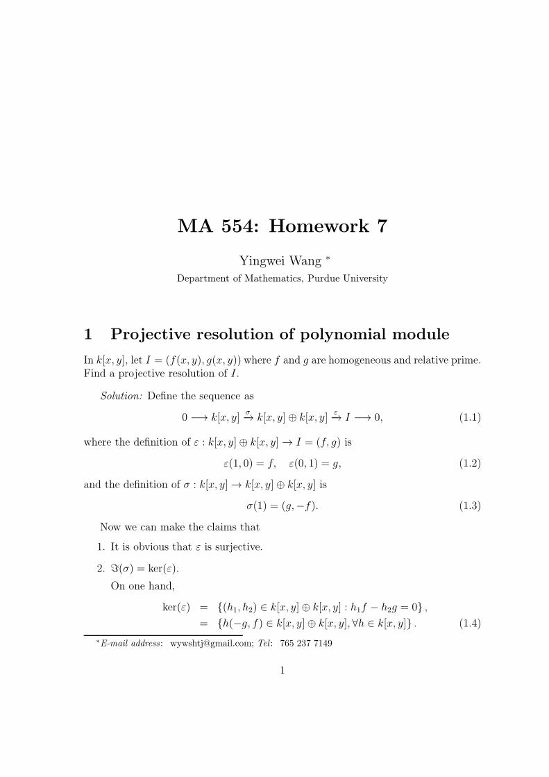
In k[x, y], let I = (f(x, y), g(x, y)) where f and g are homogeneous and relative prime.Find a projective resolution of I.
Solution: Define the sequence as
0 −→ k[x, y]σ
−→ k[x, y]⊕ k[x, y]ε
−→ I −→ 0, (1.1)
where the definition of ε : k[x, y]⊕ k[x, y] → I = (f, g) is
ε(1, 0) = f, ε(0, 1) = g, (1.2)
and the definition of σ : k[x, y] → k[x, y]⊕ k[x, y] is
σ(1) = (g,−f). (1.3)
Now we can make the claims that
1. It is obvious that ε is surjective.
2. ℑ(σ) = ker(ε).
On one hand,
ker(ε) = {(h1, h2) ∈ k[x, y]⊕ k[x, y] : h1f − h2g = 0} ,
= {h(−g, f) ∈ k[x, y]⊕ k[x, y], ∀h ∈ k[x, y]} . (1.4)
∗E-mail address : [email protected]; Tel : 765 237 7149
1
Yingwei Wang Linear Algebra
One the other hand,
ℑ(σ) = {h(−g, f) ∈ k[x, y]⊕ k[x, y], ∀h ∈ k[x, y]} . (1.5)
3. It is obvious that both k[x, y] and k[x, y]⊕ k[x, y] are projective.
Now we know that (1.1) is a projective resolution of I.
2 Idempotent
Proposition 2.1. Let e be idempotent, i.e. e2 = e. Then eR is a projective module.
Proof. Just need to show that
eR ⊕ (1− e)R ≃ R. (2.1)
1. ∀r ∈ R, r = er + (1− e)r
2. eR ∩ (1− e)R = {0}.
Since ∀x ∈ eR ∩ (1− e)R, we have
ex = (1− e)x,
⇒ e2x = e(1− e)x = (e− e2)x = 0,
⇒ x = 0.
Now we are done.
3 Z-module
Proposition 3.1. The Q is not a projective Z-module.
Proof. Let us take the first step in the free resolution of Q:
f0 : M ։ Q, (3.1)
where M is a free Z-module. Besides, let
i : Q → Q. (3.2)
be the identity map. Then we have the following diagram:
2
Yingwei Wang Linear Algebra
Now we just need to show that there is no map
φ : Q → M, (3.3)
(as indicated by the dashed arrow in the following diagram) such that the diagramcommutes.
Let us prove this by contradiction. Suppose φ : Q → M were such a map. Then
φ(1) = (a1, a2, · · · , an, 0, · · · ),
for some a1, a2, · · · , an ∈ Z. Let
a = max{a1, a2, · · · , an}.
Then
(a1, a2, · · · , an, 0, · · · ) = φ(1) = φ
(
a+ 1
a+ 1
)
= (a+ 1)φ
(
1
a + 1
)
.
It indicates that a + 1 must divide each of a1, a2, · · · , an. However, since a + 1 > aifor each i = 1, 2, · · · , n, this is impossible.
Therefore, there is no such φ. Hence, Q is not a projective Z module.
3
MA 554: Homework 9
Yingwei Wang ∗
Department of Mathematics, Purdue University
1 Baer sum
Definition 1.1. Given two extensions
0 −→ Dσ1−→ E1
µ1
−→ M −→ 0, (1.1)
0 −→ Dσ2−→ E2
µ2
−→ M −→ 0, (1.2)
(1.3)
we can construct the Baer sum as following.
Let
A = {(a1, a2) : µ1(a1) = µ2(a2)} ⊂ E1 ⊕ E2, (1.4)
B = {(d1, d2) : ∃d ∈ D such that σ1(d) = d1, σ2(−d) = d2} , (1.5)
C = σ1D ⊕ σ2D. (1.6)
Then
C/B ≃ D, A/C ≃M. (1.7)
And the extension
0 −→ C/B −→ A/B −→ A/C −→ 0 (1.8)
is called the Baer sum of the extensions E1 and E2.
Proposition 1.1. Consider the extension
0 −→ Z2−→ Z
π−→ Z/2Z −→ 0. (1.9)
∗E-mail address : [email protected]; Tel : 765 237 7149
1
Yingwei Wang Linear Algebra
Let E1 = E2 = Z, then the Baer sum of extensions E1 and E2 is
0 −→ Z −→ Z⊕ Z/2Z −→ Z/2Z −→ 0. (1.10)
Proof. By Definition 1.1, we can define
A = {(even, even)} ∪ {(odd, odd)} ⊂ Z⊕ Z, (1.11)
B = {(2n,−2n) : n ∈ Z} , (1.12)
C = 2Z⊕ 2Z. (1.13)
1. Claim that C/B ≃ Z.
Define the map ϕ1 : C −→ Z as
ϕ1(2n, 2m) = 2n− 2m. (1.14)
It is easy to know that ϕ1 is a surjective homomorphism and kerϕ1 = B. Itfollows that
C/B ≃ Z. (1.15)
2. Claim that A/C ≃ Z/2Z.
Define the map ϕ2 : A −→ Z/2Z as
ϕ2(n,m) = n, mod 2. (1.16)
It is easy to know that ϕ2 is a surjective homomorphism and kerϕ2 = C. Itfollows that
A/C ≃ Z/2Z. (1.17)
3. Claim that A/B ≃ Z⊕ Z/2Z.
Define the map ϕ3 : A −→ Z⊕ Z/2Z as
ϕ3(a1, a2) =
(
a1 + a22
, a1 mod 2
)
. (1.18)
It is easy to know that ϕ3 is a surjective homomorphism and kerϕ3 = B. Itfollows that
A/B ≃ Z/2Z. (1.19)
Now it is clear that the Baer sum of extensions E1 and E2 is
0 −→ Z −→ Z⊕ Z/2Z −→ Z/2Z −→ 0. (1.20)
2
Yingwei Wang Linear Algebra
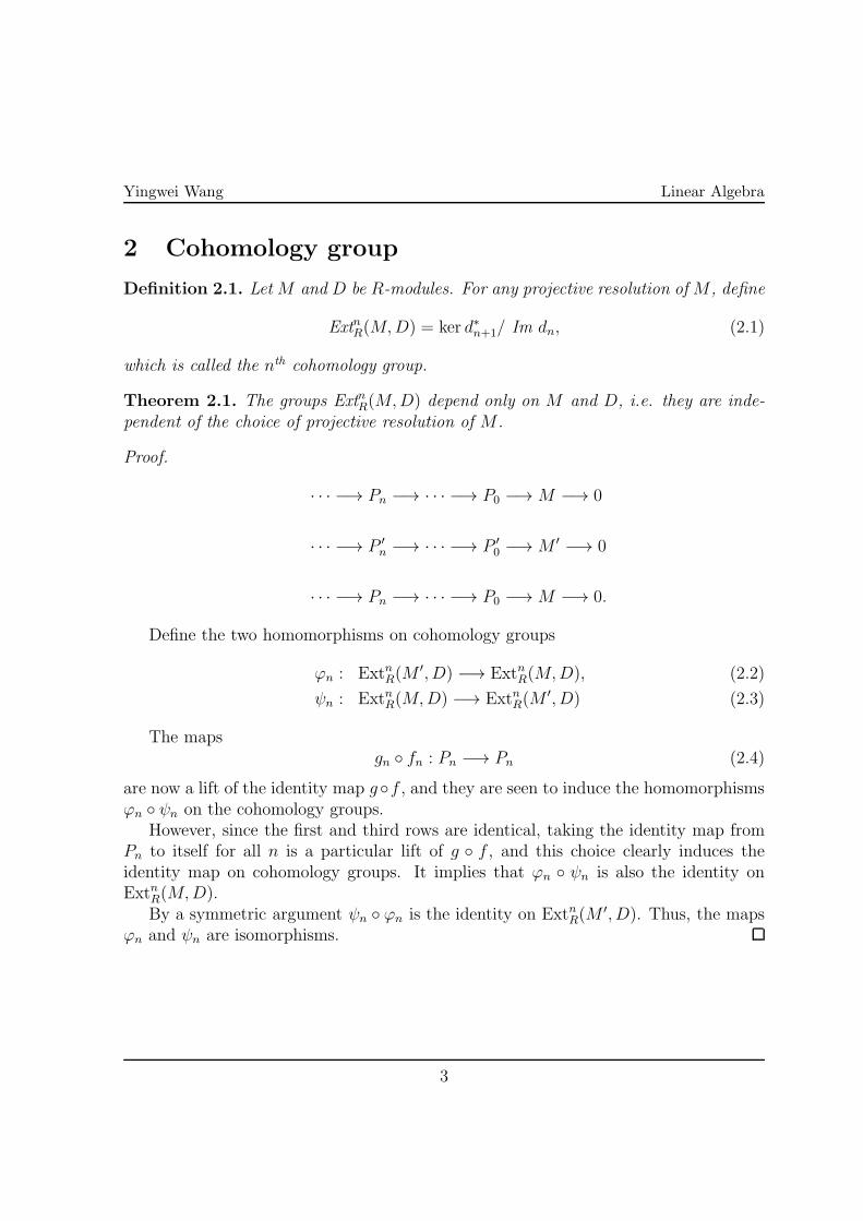
2 Cohomology group
Definition 2.1. LetM and D be R-modules. For any projective resolution ofM , define
ExtnR(M,D) = ker d∗n+1/ Im dn, (2.1)
which is called the nth cohomology group.
Theorem 2.1. The groups ExtnR(M,D) depend only on M and D, i.e. they are inde-
pendent of the choice of projective resolution of M .
Proof.
· · · −→ Pn −→ · · · −→ P0 −→ M −→ 0
· · · −→ P ′
n −→ · · · −→ P ′
0 −→ M ′ −→ 0
· · · −→ Pn −→ · · · −→ P0 −→ M −→ 0.
Define the two homomorphisms on cohomology groups
ϕn : ExtnR(M′, D) −→ ExtnR(M,D), (2.2)
ψn : ExtnR(M,D) −→ ExtnR(M′, D) (2.3)
The mapsgn ◦ fn : Pn −→ Pn (2.4)
are now a lift of the identity map g◦f , and they are seen to induce the homomorphismsϕn ◦ ψn on the cohomology groups.
However, since the first and third rows are identical, taking the identity map fromPn to itself for all n is a particular lift of g ◦ f , and this choice clearly induces theidentity map on cohomology groups. It implies that ϕn ◦ ψn is also the identity onExtnR(M,D).
By a symmetric argument ψn ◦ ϕn is the identity on ExtnR(M′, D). Thus, the maps
ϕn and ψn are isomorphisms.
3
MA 554: Homework 10
Yingwei Wang ∗
Department of Mathematics, Purdue University
1 x-adic norm
Definition 1.1 (Formal power series ring). Define the formal power series ring over
the field k as follows
k[[x]] = {∑
j≥0
ajxj , aj ∈ k}. (1.1)
Definition 1.2 (x-adic norm). Define the x-adic norm over the ring k[[x]] as follows
∀f(x) ∈ k[[x]], |f(x)| = 2−ordxf , (1.2)
where ordxf is the maximum integer such that xe divides the polynomial f(x).
Remark 1.1. In the definition (1.2), the constant 2 is irrelevant, and could be replaced
by any real number greater than 1.
Definition 1.3 (x-adic distance). Define the x-adic distance between two elements
f, g ∈ k[[x]] as follows
d(f, g) = |f − g| = 2−ordx(f−g). (1.3)
Remark 1.2. It is easy to know that
d(0, f) = |f |, ∀f(x) ∈ k[[x]]. (1.4)
∗E-mail address : [email protected]; Tel : 765 237 7149
1
Yingwei Wang Linear Algebra
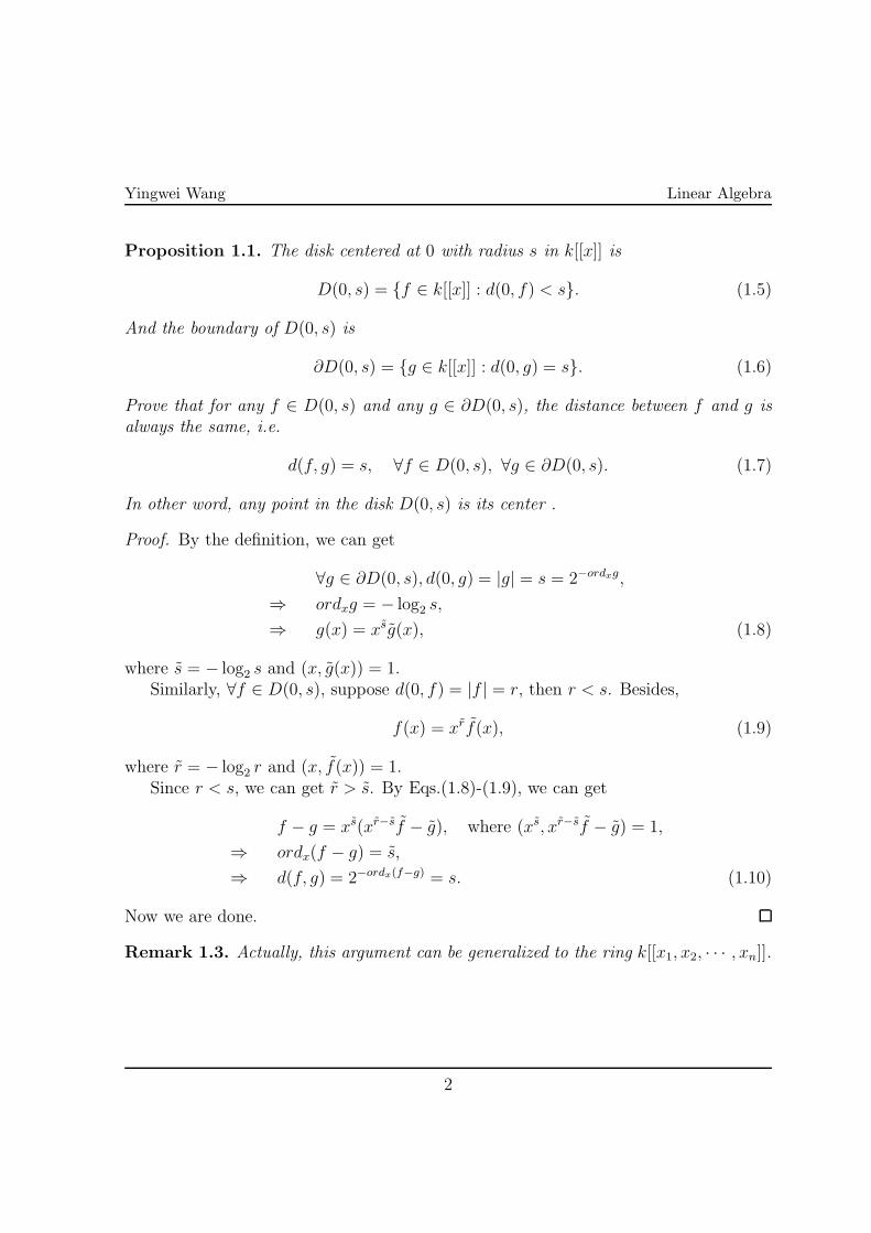
Proposition 1.1. The disk centered at 0 with radius s in k[[x]] is
D(0, s) = {f ∈ k[[x]] : d(0, f) < s}. (1.5)
And the boundary of D(0, s) is
∂D(0, s) = {g ∈ k[[x]] : d(0, g) = s}. (1.6)
Prove that for any f ∈ D(0, s) and any g ∈ ∂D(0, s), the distance between f and g is
always the same, i.e.
d(f, g) = s, ∀f ∈ D(0, s), ∀g ∈ ∂D(0, s). (1.7)
In other word, any point in the disk D(0, s) is its center .
Proof. By the definition, we can get
∀g ∈ ∂D(0, s), d(0, g) = |g| = s = 2−ordxg,
⇒ ordxg = − log2 s,
⇒ g(x) = xsg(x), (1.8)
where s = − log2 s and (x, g(x)) = 1.Similarly, ∀f ∈ D(0, s), suppose d(0, f) = |f | = r, then r < s. Besides,
f(x) = xrf(x), (1.9)
where r = − log2 r and (x, f(x)) = 1.Since r < s, we can get r > s. By Eqs.(1.8)-(1.9), we can get
f − g = xs(xr−sf − g), where (xs, xr−sf − g) = 1,
⇒ ordx(f − g) = s,
⇒ d(f, g) = 2−ordx(f−g) = s. (1.10)
Now we are done.
Remark 1.3. Actually, this argument can be generalized to the ring k[[x1, x2, · · · , xn]].
2
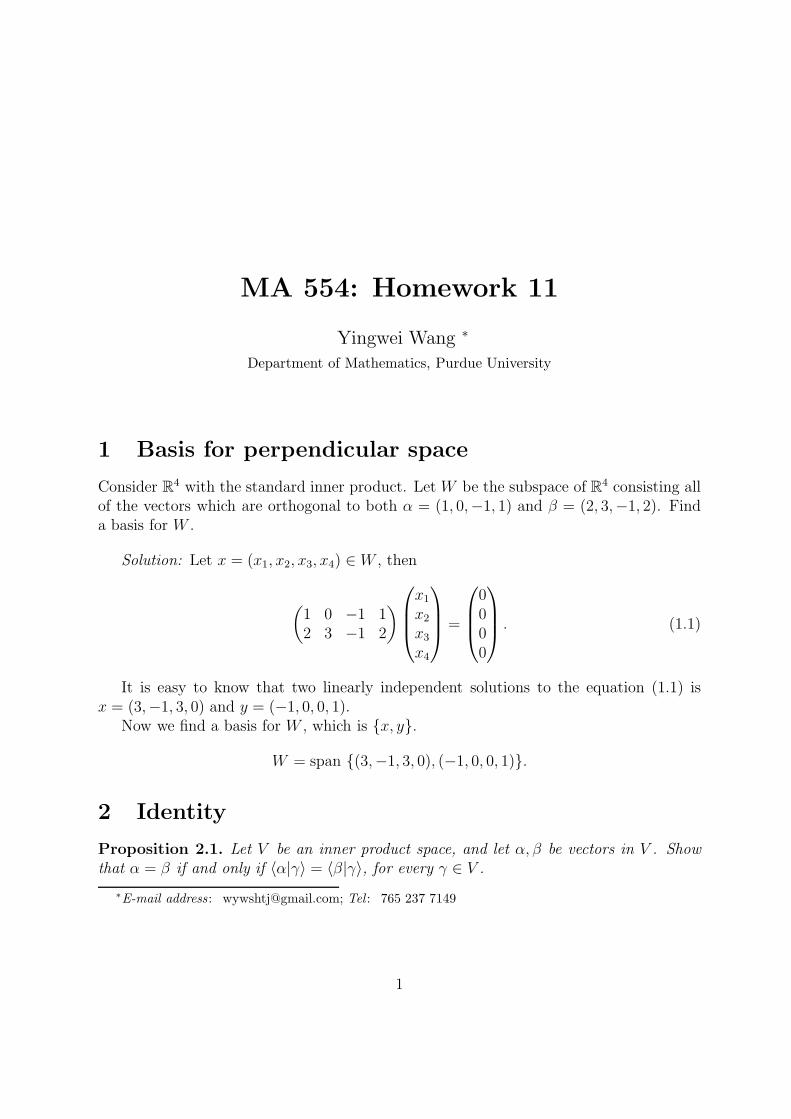
MA 554: Homework 11
Yingwei Wang ∗
Department of Mathematics, Purdue University
1 Basis for perpendicular space
Consider R4 with the standard inner product. Let W be the subspace of R4 consisting allof the vectors which are orthogonal to both α = (1, 0,−1, 1) and β = (2, 3,−1, 2). Finda basis for W .
Solution: Let x = (x1, x2, x3, x4) ∈ W , then
(
1 0 −1 12 3 −1 2
)
x1
x2
x3
x4
=
0000
. (1.1)
It is easy to know that two linearly independent solutions to the equation (1.1) isx = (3,−1, 3, 0) and y = (−1, 0, 0, 1).
Now we find a basis for W , which is {x, y}.
W = span {(3,−1, 3, 0), (−1, 0, 0, 1)}.
2 Identity
Proposition 2.1. Let V be an inner product space, and let α, β be vectors in V . Show
that α = β if and only if 〈α|γ〉 = 〈β|γ〉, for every γ ∈ V .
∗E-mail address : [email protected]; Tel : 765 237 7149
1
Yingwei Wang Linear Algebra
Proof. 1. ⇒): Suppose α = β, then
α = β,
⇒ α− β = 0,
⇒ 〈α− β|γ〉 = 0, ∀γ ∈ V,
⇒ 〈α|γ〉 − 〈β|γ〉 = 0, ∀γ ∈ V,
⇒ 〈α|γ〉 = 〈β|γ〉, ∀γ ∈ V.
2. Suppose 〈α|γ〉 = 〈β|γ〉, for every γ ∈ V , then
〈α|γ〉 = 〈β|γ〉, ∀γ ∈ V,
⇒ 〈α|γ〉 − 〈β|γ〉 = 0, ∀γ ∈ V,
⇒ 〈α− β|γ〉 = 0, ∀γ ∈ V,
⇒ α− β = 0,
⇒ α = β.
3 New inner product in R2
Let V be the inner product space consisting of R2 and the inner product whose quadraticform is defined by
‖(x1, x2)‖2 = (x1 − x2)2 + 3x2
2. (3.1)
The inner product consisting of this norm is
〈x|y〉 = (x1 − x2)(y1 − y2) + 3x2y2, (3.2)
where x = (x1, x2), y = (y1, y2) ∈ V .Let E be the orthogonal projection of V onto the subspace W spanned by the vector
(3, 4). Now do the following things.
1. Find a formula for E(x1, x2).
By Eq.(3.1), it is easy to know that ‖(3, 4)‖ = 7. Let e1 =(3,4)
‖(3,4)‖ =(
37, 47
)
, which isa normalized basis for W .
2

Yingwei Wang Linear Algebra
Now let us do the projection.
E(x1, x2) = 〈x|e1〉e1,
=
(
(x1 − x2)
(
3
7− 4
7
)
+ 3x24
7
)(
3
7,4
7
)
,
=
(
−1
7x1 +
13
7x2
)(
3
7,4
7
)
,
=
(
− 3
49x1 +
39
49x2,−
4
49x1 +
52
49x2
)
. (3.3)
2. Find the matrix of E in the standard ordered basis.
By Eq.(3.3), we know that
[
− 349
3949
− 449
5249
](
x1
x2
)
=
(
− 349x1 +
3949x2
− 449x1 +
5249x2
)
. (3.4)
It follows that the matrix form of E is[
− 349
3949
− 449
5249
]
. (3.5)
3. Find W⊥.
We just need to find e2 ∈ V such that 〈e1|e2〉 = 0 and ‖e2‖ = 1.
Let e2 = (z1, z2), then 〈e1|e2〉 = 0 implies that −(z1 − z2)17+ 3z2
47= 0, which leads
to z1 = 13z2. After normalization, we can get e2 =1√147
(13, 1).
Now we know that W⊥ = span {e2}, where e2 =1√147
(13, 1).
4. Find an orthonormal basis in which E is represented by the matrix
[
1 00 0
]
. (3.6)
Just choose the set {e1, e2} as an orthonormal basis of V . Then E is equivalent tothe matrix (3.6).
3
Yingwei Wang Linear Algebra
4 Polynomial space
Let V be the subspace of R[x] of polynomials of degree at most 3. Equip V with theinner product
〈f |g〉 =∫ 1
0
f(t)g(t)dt. (4.1)
1. Find the orthogonal complement of the subspace of scalar polynomial.
Let W = span {1} be the scalar polynomial space and p(x) ∈ W⊥, where p(x) =a3x
3 + a2x2 + a1x+ a0. Then
〈p|1〉 =∫ 1
0
p(x)dx = 0,
⇒ 1
4a3 +
1
3a2 +
1
2a1 + a0 = 0,
⇒ a0 = −1
4a3 −
1
3a2 −
1
2a1.
It follows that the basis for W⊥ can be chosen as
p1(x) = x− 1
2, p2(x) = x2 − 1
3, p3(x) = x3 − 1
4.
That is to say, W⊥ = {x− 12, x2 − 1
3, x3 − 1
4}.
2. Apply the Gram-Schmidt process to the basis {1, x, x2, x3}.
(a) Let v1 = 1, then w1 =v1
‖v1‖ = 1.
(b) Let v2 = x, then
v2 − 〈v2|w1〉w1 = x− 1
2,
⇒ w2 =x− 1
2
‖x− 12‖ = 2
√3
(
x− 1
2
)
.
(c) Let v3 = x2, then
v3 − 〈v3|w1〉w1 − 〈v3|w2〉w2 = x2 − x+1
6,
⇒ w3 =x2 − x+ 1
6
‖x2 − x+ 16‖ = 6
√5
(
x2 − x+1
6
)
.
4
Yingwei Wang Linear Algebra
(d) Let v4 = x3, then
v4 − 〈v4|w1〉w1 − 〈v4|w2〉w2 − 〈v4|w3〉w3 = x3 − 3
2x2 +
3
5x− 1
20,
⇒ w4 =x3 − 3
2x2 + 3
5x− 1
20
‖x3 − 32x2 + 3
5x− 1
20‖ = 20
√7
(
x3 − 3
2x2 +
3
5x− 1
20
)
.
In conclusion, we get an orthonormal basis, V = span {w1, w2, w3, w4}.
5 Perpendicular space
Proposition 5.1. Let S be a subset of an inner product space V . Show that (S⊥)⊥
contains the subspace spanned by S. When V is finite-dimensional, show that (S⊥)⊥ is
the subspace spanned by S.
Proof. Let S = span{S}.
1. Claim that (S⊥)⊥ ⊃ S.
For ∀α ∈ S, ∀β ∈ S⊥,
β ∈ S⊥,
⇒ 〈β|s〉 = 0, ∀s ∈ S,
⇒ 〈β|α〉 = 0, ∀α ∈ S,
⇒ α ∈ (S⊥)⊥.
It follows that (S⊥)⊥ ⊃ S.
2. Claim that if V is finite-dimensional, then (S⊥)⊥ = S.
Suppose dim(V ) = n and dim(S) = k, where k ≤ n. By theorem 5 in the textbook,we know that
dim(S⊥) = n− k,
⇒ dim((S⊥)⊥) = n− (n− k) = k.
It follows that dim((S⊥)⊥) = dim(S). Besides, since we know that (S⊥)⊥ ⊃ S, thenwe can conclude that (S⊥)⊥ = S.
5
Yingwei Wang Linear Algebra
6 Odd and even functions
Let V be the real value inner product space consisting of the space of real-valued contin-uous functions on the interval −1 ≤ t ≤ 1, with the inner product
〈f |g〉 =∫ 1
−1
f(t)g(t)dt. (6.1)
Let W be the subspace of odd functions, i.e. functions satisfying f(−t) = f(t). Find theorthogonal complement of W .
Solution:
Choose ∀g ∈ W⊥ and define the two functions
g1(t) =g(t) + g(−t)
2,
g2(t) =g(t)− g(−t)
2.
It is easy to know that g1(t) is an even function and g2(t) is an odd function. Besides,g(t) can be written as the sum of two parts, i.e.
g(t) = g1(t) + g2(t). (6.2)
Let f ∈ W , then
〈f |g〉 = 0,
⇒∫ 1
−1
f(t)g1(t)dt+
∫ 1
−1
f(t)g2(t)dt = 0,
⇒∫ 1
−1
f(t)g2(t)dt = 0, (since f(t)g1(t) is odd),
⇒ f(t)g2(t) = 0, (since f(t)g2(t) is even),
⇒ g2(t) = 0, (since f(t) is arbitrary).
Now it is clear that ∀g ∈ W⊥, g must be an even function. In other word, W⊥ is thesubspace of odd functions.
6

MA 554: Homework 12
Yingwei Wang ∗
Department of Mathematics, Purdue University
1 Adjoint operator
Proposition 1.1. Let V be an inner product space and β, γ fixed vectors in V . Show that
Tα = 〈α|β〉γ defines a linear operator on V . Show that T has an adjoint, and describe
T ∗ explicitly.
Now suppose V is Cn with the standard inner product, β = (y1, · · · , yn) be row vectors,
and γ = (z1, · · · , zn). What is the j, k entry of the matrix of T in the standard ordered
basis? What is the rank of the matrix?
Proof. On one hand, by the definition of adjoint operator, we can get
〈Tα|w〉 = 〈α|T ∗w〉, (1.1)
for any α,w ∈ V .On the other hand, by the definition of T , we can get
〈Tα|w〉 = 〈α|β〉〈γ|w〉,
= 〈α|(
〈γ|w〉)
β〉,
= 〈α| (〈w|γ〉) β〉. (1.2)
By Eqs.(1.1)-(1.2), we can get
T ∗w = 〈w|γ〉β, ∀w ∈ V. (1.3)
Furthermore, let {e1, e2, · · · , en} be the standard ordered basis. Then
Tej = 〈ej|β〉γ = yjγ,
⇒ the matrix of T = βTγ.
Besides, the rank of this matrix is 1.
∗E-mail address : [email protected]; Tel : 765 237 7149
1
Yingwei Wang Linear Algebra
2 Self-adjoint operators
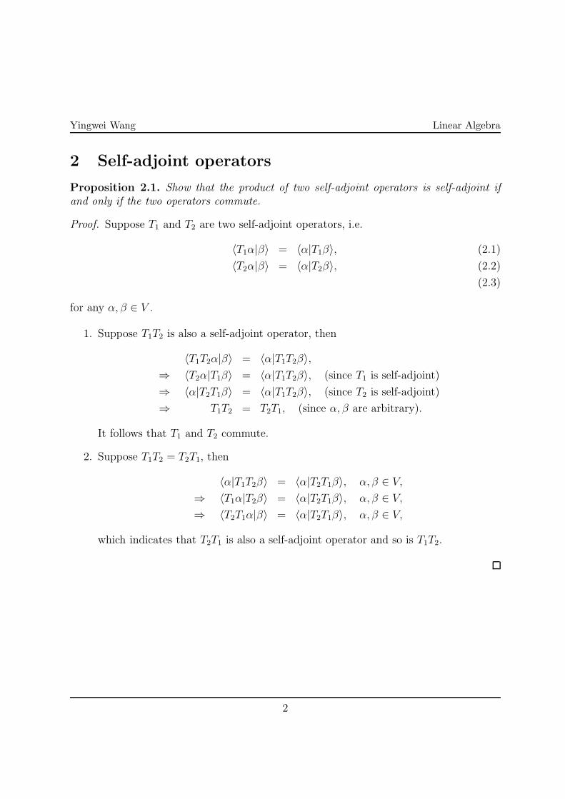
Proposition 2.1. Show that the product of two self-adjoint operators is self-adjoint if
and only if the two operators commute.
Proof. Suppose T1 and T2 are two self-adjoint operators, i.e.
〈T1α|β〉 = 〈α|T1β〉, (2.1)
〈T2α|β〉 = 〈α|T2β〉, (2.2)
(2.3)
for any α, β ∈ V .
1. Suppose T1T2 is also a self-adjoint operator, then
〈T1T2α|β〉 = 〈α|T1T2β〉,
⇒ 〈T2α|T1β〉 = 〈α|T1T2β〉, (since T1 is self-adjoint)
⇒ 〈α|T2T1β〉 = 〈α|T1T2β〉, (since T2 is self-adjoint)
⇒ T1T2 = T2T1, (since α, β are arbitrary).
It follows that T1 and T2 commute.
2. Suppose T1T2 = T2T1, then
〈α|T1T2β〉 = 〈α|T2T1β〉, α, β ∈ V,
⇒ 〈T1α|T2β〉 = 〈α|T2T1β〉, α, β ∈ V,
⇒ 〈T2T1α|β〉 = 〈α|T2T1β〉, α, β ∈ V,
which indicates that T2T1 is also a self-adjoint operator and so is T1T2.
2
Yingwei Wang Linear Algebra
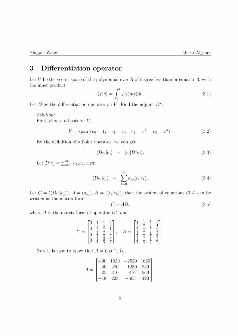
3 Differentiation operator
Let V be the vector space of the polynomial over R of degree less than or equal to 3, withthe inner product
〈f |g〉 =
∫
1
0
f(t)g(t)dt. (3.1)
Let D be the differentiation operator on V . Find the adjoint D∗.
Solution:
First, choose a basis for V ,
V = span {e0 = 1, e1 = x, e2 = x2, e3 = x3}. (3.2)
By the definition of adjoint operator, we can get
〈Dei|ej〉 = 〈ei|D∗ej〉. (3.3)
Let D∗ej =∑
3
k=0akjek, then
〈Dei|ej〉 =3
∑
k=0
akj〈ei|ek〉. (3.4)
Let C = (〈Dei|ej〉), A = (akj), B = (〈ei|ek〉), then the system of equations (3.4) can bewritten as the matrix form
C = AB, (3.5)
where A is the matrix form of operator D∗, and
C =
0 1 1 3
2
0 1
2
2
31
0 1
3
1
2
3
4
0 1
4
2
5
3
5
, B =
1 1
2
1
3
1
41
2
1
3
1
4
1
51
3
1
4
1
5
1
61
4
1
5
1
6
1
7
.
Now it is easy to know that A = CB−1, i.e.
A =
−90 1020 −2520 1680−40 480 −1230 840−25 310 −810 560−18 228 −603 420
.
3
Yingwei Wang Linear Algebra
4 Self-adjoint unitary operator: a particular case
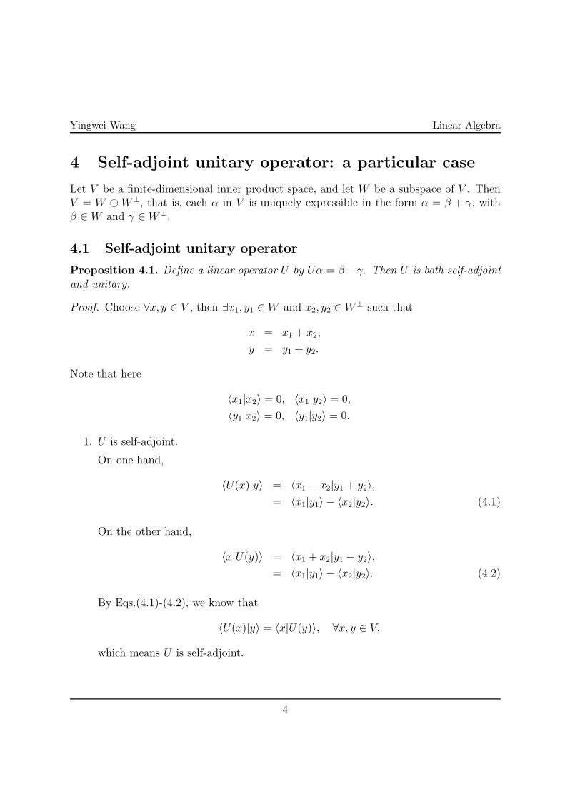
Let V be a finite-dimensional inner product space, and let W be a subspace of V . ThenV = W ⊕W⊥, that is, each α in V is uniquely expressible in the form α = β + γ, withβ ∈ W and γ ∈ W⊥.
4.1 Self-adjoint unitary operator
Proposition 4.1. Define a linear operator U by Uα = β−γ. Then U is both self-adjoint
and unitary.
Proof. Choose ∀x, y ∈ V , then ∃x1, y1 ∈ W and x2, y2 ∈ W⊥ such that
x = x1 + x2,
y = y1 + y2.
Note that here
〈x1|x2〉 = 0, 〈x1|y2〉 = 0,
〈y1|x2〉 = 0, 〈y1|y2〉 = 0.
1. U is self-adjoint.
On one hand,
〈U(x)|y〉 = 〈x1 − x2|y1 + y2〉,
= 〈x1|y1〉 − 〈x2|y2〉. (4.1)
On the other hand,
〈x|U(y)〉 = 〈x1 + x2|y1 − y2〉,
= 〈x1|y1〉 − 〈x2|y2〉. (4.2)
By Eqs.(4.1)-(4.2), we know that
〈U(x)|y〉 = 〈x|U(y)〉, ∀x, y ∈ V,
which means U is self-adjoint.
4
Yingwei Wang Linear Algebra
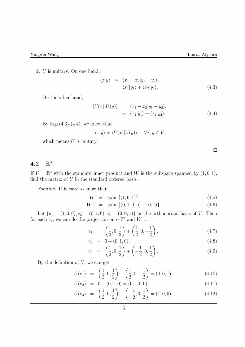
2. U is unitary. On one hand,
〈x|y〉 = 〈x1 + x2|y1 + y2〉,
= 〈x1|y1〉+ 〈x2|y2〉. (4.3)
On the other hand,
〈U(x)|U(y)〉 = 〈x1 − x2|y1 − y2〉,
= 〈x1|y1〉+ 〈x2|y2〉. (4.4)
By Eqs.(4.3)-(4.4), we know that
〈x|y〉 = 〈U(x)|U(y)〉, ∀x, y ∈ V,
which means U is unitary.
4.2 R3
If V = R3 with the standard inner product and W is the subspace spanned by (1, 0, 1),
find the matrix of U in the standard ordered basis.
Solution: It is easy to know that
W = span {(1, 0, 1)}, (4.5)
W⊥ = span {(0, 1, 0), (−1, 0, 1)}. (4.6)
Let {e1 = (1, 0, 0), e2 = (0, 1, 0), e3 = (0, 0, 1)} be the orthonormal basis of V . Thenfor each ej, we can do the projection onto W and W⊥:
e1 =
(
1
2, 0,
1
2
)
+
(
1
2, 0,−
1
2
)
, (4.7)
e2 = 0 + (0, 1, 0), (4.8)
e3 =
(
1
2, 0,
1
2
)
+
(
−1
2, 0,
1
2
)
. (4.9)
By the definition of U , we can get
U(e1) =
(
1
2, 0,
1
2
)
−
(
1
2, 0,−
1
2
)
= (0, 0, 1), (4.10)
U(e2) = 0− (0, 1, 0) = (0,−1, 0), (4.11)
U(e3) =
(
1
2, 0,
1
2
)
−
(
−1
2, 0,
1
2
)
= (1, 0, 0). (4.12)
5
Yingwei Wang Linear Algebra
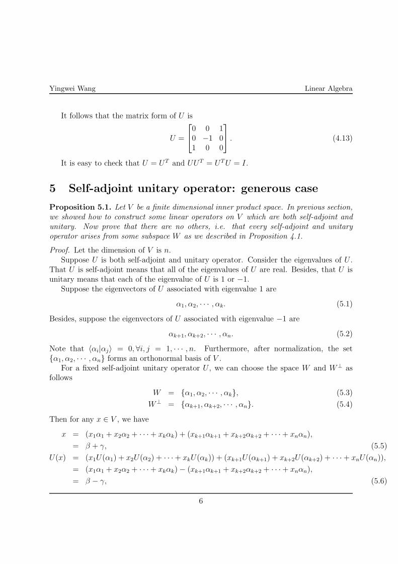
It follows that the matrix form of U is
U =
0 0 10 −1 01 0 0
. (4.13)
It is easy to check that U = UT and UUT = UTU = I.
5 Self-adjoint unitary operator: generous case
Proposition 5.1. Let V be a finite dimensional inner product space. In previous section,
we showed how to construct some linear operators on V which are both self-adjoint and
unitary. Now prove that there are no others, i.e. that every self-adjoint and unitary
operator arises from some subspace W as we described in Proposition 4.1.
Proof. Let the dimension of V is n.Suppose U is both self-adjoint and unitary operator. Consider the eigenvalues of U .
That U is self-adjoint means that all of the eigenvalues of U are real. Besides, that U isunitary means that each of the eigenvalue of U is 1 or −1.
Suppose the eigenvectors of U associated with eigenvalue 1 are
α1, α2, · · · , αk. (5.1)
Besides, suppose the eigenvectors of U associated with eigenvalue −1 are
αk+1, αk+2, · · · , αn. (5.2)
Note that 〈αi|αj〉 = 0, ∀i, j = 1, · · · , n. Furthermore, after normalization, the set{α1, α2, · · · , αn} forms an orthonormal basis of V .
For a fixed self-adjoint unitary operator U , we can choose the space W and W⊥ asfollows
W = {α1, α2, · · · , αk}, (5.3)
W⊥ = {αk+1, αk+2, · · · , αn}. (5.4)
Then for any x ∈ V , we have
x = (x1α1 + x2α2 + · · ·+ xkαk) + (xk+1αk+1 + xk+2αk+2 + · · ·+ xnαn),
= β + γ, (5.5)
U(x) = (x1U(α1) + x2U(α2) + · · ·+ xkU(αk)) + (xk+1U(αk+1) + xk+2U(αk+2) + · · ·+ xnU(αn)),
= (x1α1 + x2α2 + · · ·+ xkαk)− (xk+1αk+1 + xk+2αk+2 + · · ·+ xnαn),
= β − γ, (5.6)
6
Yingwei Wang Linear Algebra
where β ∈ W and γ ∈ W⊥.In conclusion, every self-adjoint and unitary operator arises from some subspace W
as we described in Proposition 4.1.
6 Rigid motion
If V is an inner product space, a rigid motion is any function T from V into V (notnecessary linear) such that
‖Tα− Tβ‖ = ‖α− β‖, ∀α, β ∈ V. (6.1)
One example of a rigid motion is a linear unitary operator. Another example istranslation by a fixed vector γ:
Tγ(α) = α + γ. (6.2)
6.1 Linear and unitary
Proposition 6.1. Let V be R2 with the standard inner product. Suppose T is a rigid
motion of V and that T (0) = 0. Prove that T is linear and a unitary operator.
Proof. 1. Claim that T preserve the inner product.
In Eq.(6.1), choosing β = 0 and thanks to the fact that T (0) = 0, we can get
‖Tα‖ = ‖α‖, ∀α ∈ V. (6.3)
Recall the formula
‖x− y‖2 = ‖x‖2 + ‖y‖2 − 2〈x|y〉, ∀x, y ∈ V. (6.4)
Now we can get
2〈Tx|Ty〉 = ‖Tx‖2 + ‖Ty‖2 − ‖Tx− Ty‖2,
= ‖x‖2 + ‖y‖2 − ‖x− y‖2,
= 2〈x|y〉, ∀x, y ∈ V.
7
Yingwei Wang Linear Algebra
2. T is linear.
Let us choose the standard basis in R2,
e1 = (1, 0), e2 = (0, 1).
Then, for ∀x, y ∈ V , we have
〈T (x+ y)|Tei〉 = 〈x+ y|ei〉,
= 〈x|ei〉+ 〈y|ei〉,
= 〈Tx|Tei〉+ 〈Ty|Tei〉,
= 〈Tx+ Ty|Tei〉, i = 1, 2.
It follows thatT (x+ y) = Tx+ Ty, ∀x, y ∈ V. (6.5)
Similarly, for any constant c, we have
〈T (cx)|Tei〉 = 〈cx|ei〉,
= c〈x|ei〉,
= c〈Tx|Tei〉,
which in turn yields that
T (cx) = cTx ∀ constant c and ∀x ∈ V. (6.6)
In conclusion, T is linear and a unitary operator.
6.2 Generalization
Proposition 6.2. Use the result we just proved to show that every rigid motion of R2 is
composed of a translation, followed by a unitary operator.
Proof. Let f be a rigid motion of R2, then
f(x) = f(0) + (f(x)− f(0)) . (6.7)
By Proposition 6.1, we know that g(x) = f(x)− f(0) is a unitary operator. Besides,h(x) = x+ f(0) can be view as a translation. Now by Eq.(6.7), it is clear that
f = h ◦ g, (6.8)
where h is a translation and g is a unitary operator.
8
Yingwei Wang Linear Algebra
6.3 Further generalization
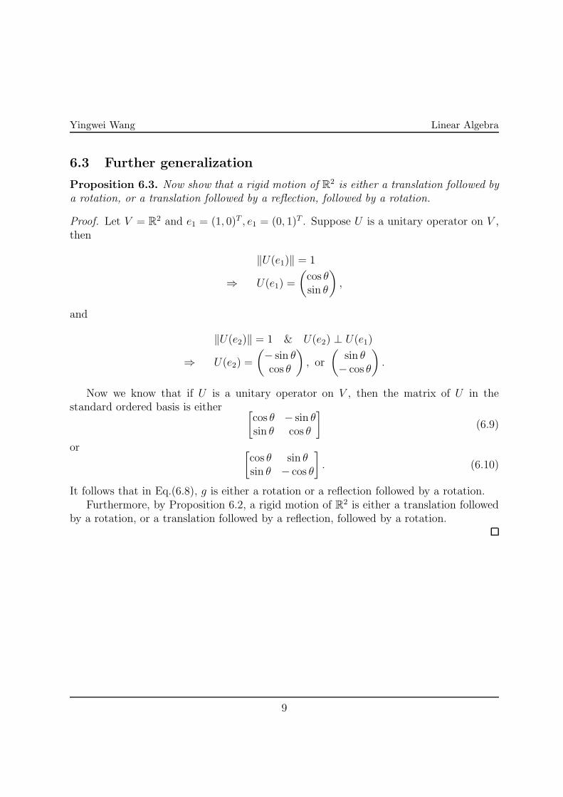
Proposition 6.3. Now show that a rigid motion of R2 is either a translation followed by
a rotation, or a translation followed by a reflection, followed by a rotation.
Proof. Let V = R2 and e1 = (1, 0)T , e1 = (0, 1)T . Suppose U is a unitary operator on V ,
then
‖U(e1)‖ = 1
⇒ U(e1) =
(
cos θsin θ
)
,
and
‖U(e2)‖ = 1 & U(e2) ⊥ U(e1)
⇒ U(e2) =
(
− sin θcos θ
)
, or
(
sin θ− cos θ
)
.
Now we know that if U is a unitary operator on V , then the matrix of U in thestandard ordered basis is either
[
cos θ − sin θsin θ cos θ
]
(6.9)
or[
cos θ sin θsin θ − cos θ
]
. (6.10)
It follows that in Eq.(6.8), g is either a rotation or a reflection followed by a rotation.Furthermore, by Proposition 6.2, a rigid motion of R2 is either a translation followed
by a rotation, or a translation followed by a reflection, followed by a rotation.
9
MA 554: Homework 13
Yingwei Wang ∗
Department of Mathematics, Purdue University
1 Diagonal matrix
For
A =
1 2 32 3 43 4 5
,
there is a real orthogonal matrix P such that P tAP = D is diagonal. Find such a diagonalmatrix D.
Solution: Since A is hermitian, the elements of D should be the eigenvalues of A.The characteristic polynomial of A is
χA(λ) = det(λI − A),
= λ3 − 9λ2 − 6λ,
= λ
(
λ− 9 +√105
2
)(
λ− 9−√105
2
)
. (1.1)
Hence, the matrix D is
D =
0 0 0
0 9+√105
20
0 0 9−√105
2
.
∗E-mail address : [email protected]; Tel : 765 237 7149
1
Yingwei Wang Linear Algebra
2 Normal operator
Proposition 2.1. Prove T is normal if and only if T = T1 + iT2 where T1 and T2 are
self-adjoint operators which commutes.
Proof. 1. Suppose T = T1 + iT2 is normal, where
T1 =1
2(T + T ∗),
T2 =1
2i(T − T ∗).
Then we have
TT ∗ = T ∗T,
⇒ (T1 + iT2)(Tt1 − iT t
2) = (T t1 − iT t
2)(T1 + iT2),
⇒ (T1Tt1 + T2T
t2) + i(T2T
t1 − T1T
t2) = (T t
1T1 + T t2T2) + i(T t
1T2 − T t2T1),
⇒{
T1Tt1 + T2T
t2 = T t
1T1 + T t2T2
T2Tt1 − T1T
t2 = T t
1T2 − T t2T1,
⇒ T1Tt1 = T t
1T1 = I, T2Tt2 = T t
2T2 = I, T1T2 = T2T1.
It follows that T1 and T2 are self-adjoint operators which commutes.
2. Suppose T = T1 + iT2, where T1 and T2 are self-adjoint operators and commuteswith each other. Then
T1Tt1 = T t
1T1 = I, T2Tt2 = T t
2T2 = I, T1T2 = T2T1. (2.1)
On one hand,
TT ∗ = (T1 + iT2)(Tt1 − iT t
2),
= (T1Tt1 + T2T
t2) + i(T2T
t1 − T1T
t2). (2.2)
On the other hand,
T ∗T = (T t1 − iT t
2)(T1 + iT2),
= (T t1T1 + T t
2T2) + i(T t1T2 − T t
2T1). (2.3)
By Eqs.(2.1)-(2.3), we can getTT ∗ = T ∗T. (2.4)
It follows that T is normal.
2
Yingwei Wang Linear Algebra
3 Normal operator
Proposition 3.1. Let T be a normal operator on a finite-dimensional complex inner
product space. Prove that there is a polynomial f , with complex coefficients, such that
T ∗ = f(T ).
Proof. 1. Assume T is an n× n diagonal matrix, i.e.
T =
z1. . .
zn
, T ∗ =
z1. . .
zn
.
It is obvious that TT ∗ = T ∗T .
We need find a polynomial f(z) of degree n− 1 such that T ∗ = f(T ).
We can use the so called “Lagrange interpolating polynomial”. Let us define
fk(z) =∏
j 6=k
zkzj
z − zj,
then it is easy to know that
fk(zj) = δkj, ∀k, j = 1, 2, · · ·n.
Let
f(z) =
n∑
k=1
zkfk(z). (3.1)
Then f(z) is a polynomial of degree n− 1 which satisfies
f(zk) = zk, ∀1 < k < n.
Now we know that
f(T ) =
f(z1). . .
f(zn)
=
z1. . .
zn
= T ∗.
3
Yingwei Wang Linear Algebra
2. Assume T is not a diagonal matrix. By theorem 22 on page 317 of the textbook,we can find a unitary matrix P such that
P−1TP = Λ = diag(λ1, λ2, · · · , λn),
P−1T ∗P = Λ∗ = diag(λ1, λ2, · · · , λn).
By Part 1, we know that there exists a polynomial of degree n− 1,
f(z) = an−1zn−1 + · · ·a1z + a0,
such that
Λ∗ = f(Λ) = an−1Λn−1 + · · · a1Λ + a0,
⇒ P−1T ∗P = an−1P−1Λn−1P + · · ·a1P−1ΛP + a0,
⇒ T ∗ = an−1Tn−1 + · · · a1T + a0 = f(T ).
Now we are done.
4 Quadratic form
Let f be the form on R2 given by
f((x1, x2), (y1, y2)) = x1y1 + 4x2y2 + 2x1y2 + 2x2y1. (4.1)
Find an ordered basis in which f is represented by a diagonal matrix.
Solution: Let
A =
[
1 22 4
]
,
thenf((x1, x2), (y1, y2)) = (x1, x2)A(y1, y2)
t.
The characteristic polynomial of A is
χA(λ) = det(λI −A),
= λ2 − 5λ,
= λ(λ− 5). (4.2)
4
Yingwei Wang Linear Algebra
It is easy to know that the eigenvalues and associated eigenvectors are
λ1 = 0, v1 =1√5(−2, 1)t,
λ2 = 5, v2 =1√5(1, 2)t.
Let
P =1√5
[
−2 11 2
]
, Λ =
[
0 00 5
]
,
then
P t = P−1,
A = PΛP t.
Let x = xP, y = yP , thenf(x, y) = xΛyt. (4.3)
Then f is represented by a diagonal matrix for the basis {v1, v2}.
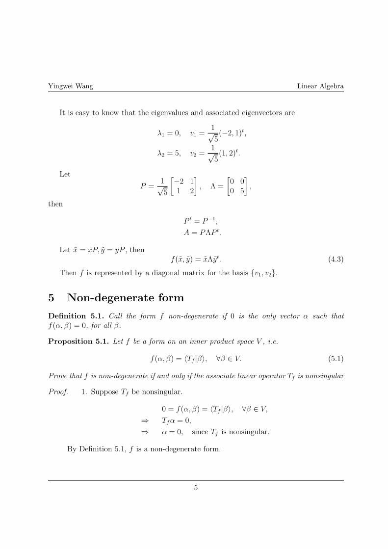
5 Non-degenerate form
Definition 5.1. Call the form f non-degenerate if 0 is the only vector α such that
f(α, β) = 0, for all β.
Proposition 5.1. Let f be a form on an inner product space V , i.e.
f(α, β) = 〈Tf |β〉, ∀β ∈ V. (5.1)
Prove that f is non-degenerate if and only if the associate linear operator Tf is nonsingular
Proof. 1. Suppose Tf be nonsingular.
0 = f(α, β) = 〈Tf |β〉, ∀β ∈ V,
⇒ Tfα = 0,
⇒ α = 0, since Tf is nonsingular.
By Definition 5.1, f is a non-degenerate form.
5
Yingwei Wang Linear Algebra
2. Let f be a non-degenerate form.
Assume Tf is singular, then we have
∃α 6= 0, such that Tfα = 0,
⇒ 〈Tf |β〉, ∀β ∈ V,
⇒ f(α, β) = 〈Tf |β〉, ∀β ∈ V.
This contradicts the fact that f is a non-degenerate form.
Hence, Tf should be nonsingular.
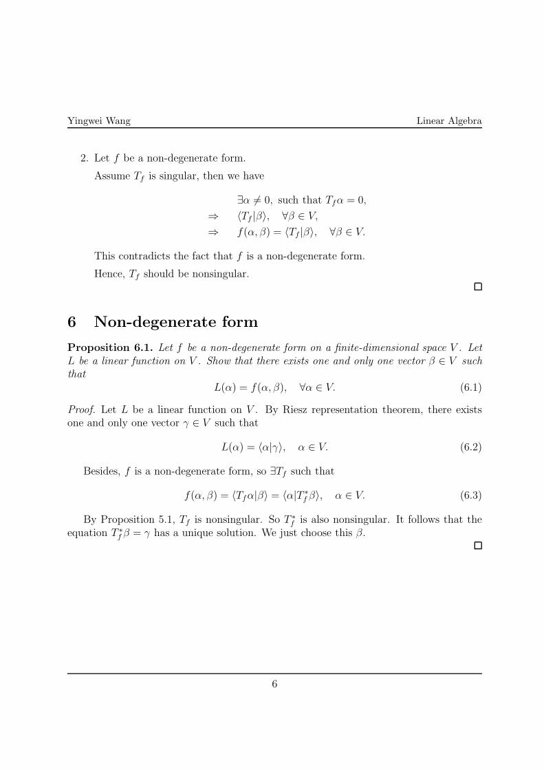
6 Non-degenerate form
Proposition 6.1. Let f be a non-degenerate form on a finite-dimensional space V . Let
L be a linear function on V . Show that there exists one and only one vector β ∈ V such
that
L(α) = f(α, β), ∀α ∈ V. (6.1)
Proof. Let L be a linear function on V . By Riesz representation theorem, there existsone and only one vector γ ∈ V such that
L(α) = 〈α|γ〉, α ∈ V. (6.2)
Besides, f is a non-degenerate form, so ∃Tf such that
f(α, β) = 〈Tfα|β〉 = 〈α|T ∗f β〉, α ∈ V. (6.3)
By Proposition 5.1, Tf is nonsingular. So T ∗f is also nonsingular. It follows that the
equation T ∗f β = γ has a unique solution. We just choose this β.
6
MA 554: Homework 14
Yingwei Wang ∗
Department of Mathematics, Purdue University
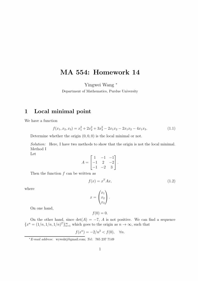
1 Local minimal point
We have a function
f(x1, x2, x3) = x2
1+ 2x2
2+ 3x2
3− 2x1x2 − 2x1x2 − 4x1x3. (1.1)
Determine whether the origin (0, 0, 0) is the local minimal or not.
Solution: Here, I have two methods to show that the origin is not the local minimal.Method ILet
A =
1 −1 −1−1 2 −2−1 −2 3
.
Then the function f can be written as
f(x) = xTAx, (1.2)
where
x =
x1
x2
x3
.
On one hand,f(0) = 0.
On the other hand, since det(A) = −7, A is not positive. We can find a sequence{xn = (1/n, 1/n, 1/n)T}∞n=1
which goes to the origin as n → ∞, such that
f(xn) = −2/n2 < f(0), ∀n.∗E-mail address : [email protected]; Tel : 765 237 7149
1
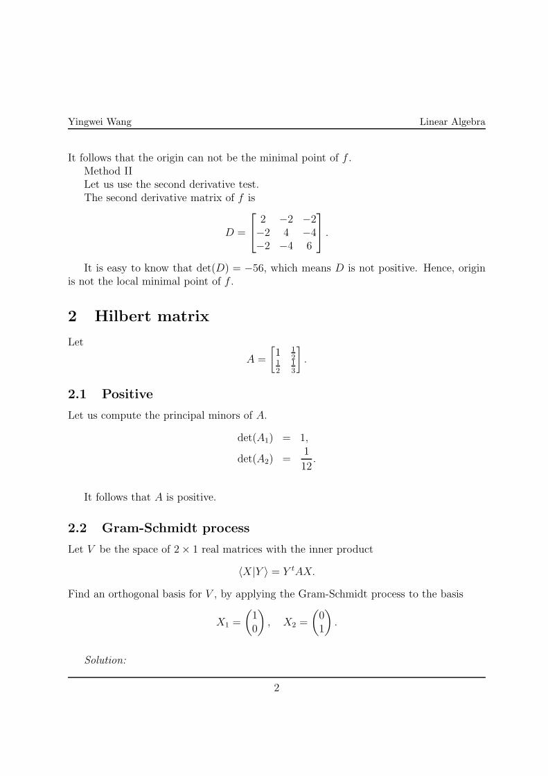
Yingwei Wang Linear Algebra
It follows that the origin can not be the minimal point of f .Method IILet us use the second derivative test.The second derivative matrix of f is
D =
2 −2 −2−2 4 −4−2 −4 6
.
It is easy to know that det(D) = −56, which means D is not positive. Hence, originis not the local minimal point of f .
2 Hilbert matrix
Let
A =
[
1 1
21
2
1
3
]
.
2.1 Positive
Let us compute the principal minors of A.
det(A1) = 1,
det(A2) =1
12.
It follows that A is positive.
2.2 Gram-Schmidt process
Let V be the space of 2× 1 real matrices with the inner product
〈X|Y 〉 = Y tAX.
Find an orthogonal basis for V , by applying the Gram-Schmidt process to the basis
X1 =
(
10
)
, X2 =
(
01
)
.
Solution:
2
Yingwei Wang Linear Algebra
e1 = X1 =
(
10
)
,
v2 = X2 − 〈X2|e1〉e1,
=
(
01
)
− 1
2
(
10
)
,
=
(
−1
2
1
)
,
e2 =v2
‖v2‖,
=
(
−√3
2√3
)
.
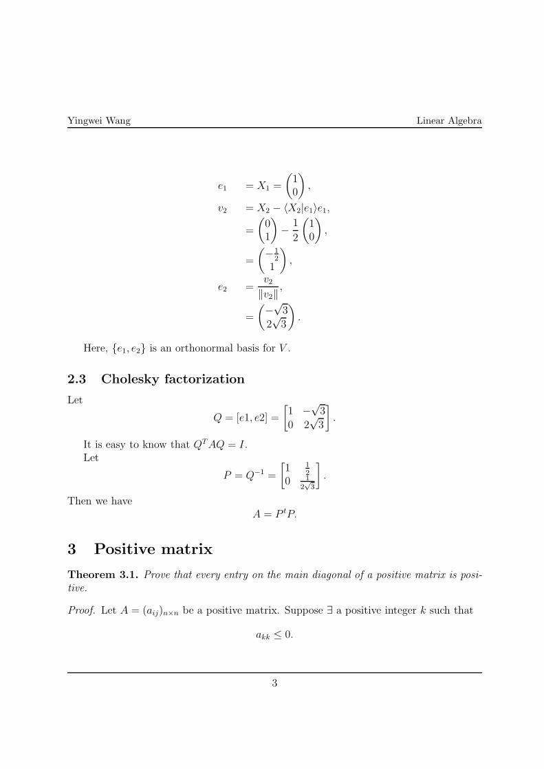
Here, {e1, e2} is an orthonormal basis for V .
2.3 Cholesky factorization
Let
Q = [e1, e2] =
[
1 −√3
0 2√3
]
.
It is easy to know that QTAQ = I.Let
P = Q−1 =
[
1 1
2
0 1
2√3
]
.
Then we haveA = P tP.
3 Positive matrix
Theorem 3.1. Prove that every entry on the main diagonal of a positive matrix is posi-tive.
Proof. Let A = (aij)n×n be a positive matrix. Suppose ∃ a positive integer k such that
akk ≤ 0.
3
Yingwei Wang Linear Algebra
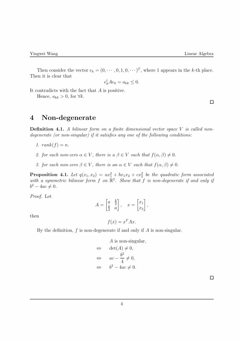
Then consider the vector ek = (0, · · · , 0, 1, 0, · · · )T , where 1 appears in the k-th place.Then it is clear that
etkAek = akk ≤ 0.
It contradicts with the fact that A is positive.Hence, akk > 0, for ∀k.
4 Non-degenerate
Definition 4.1. A bilinear form on a finite dimensional vector space V is called non-degenerate (or non-singular) if it satisfies any one of the following conditions:
1. rank(f) = n.
2. for each non-zero α ∈ V , there is a β ∈ V such that f(α, β) 6= 0.
3. for each non-zero β ∈ V , there is an α ∈ V such that f(α, β) 6= 0.
Proposition 4.1. Let q(x1, x2) = ax2
1+ bx1x2 + cx2
2be the quadratic form associated
with a symmetric bilinear form f on R2. Show that f is non-degenerate if and only if
b2 − 4ac 6= 0.
Proof. Let
A =
[
a b2
b2
a
]
, x =
[
x1
x2
]
,
thenf(x) = xTAx.
By the definition, f is non-degenerate if and only if A is non-singular.
A is non-singular,
⇔ det(A) 6= 0,
⇔ ac− b2
46= 0,
⇔ b2 − 4ac 6= 0.
4
Yingwei Wang Linear Algebra
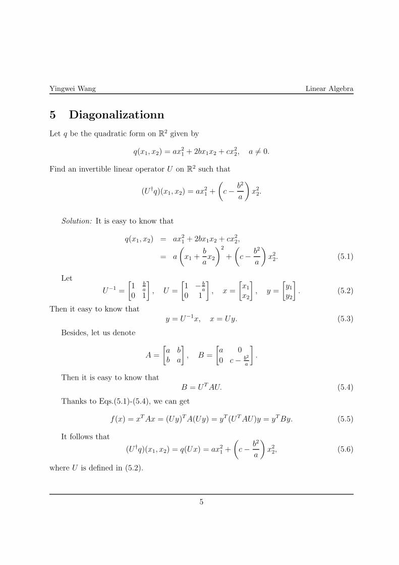
5 Diagonalizationn
Let q be the quadratic form on R2 given by
q(x1, x2) = ax2
1+ 2bx1x2 + cx2
2, a 6= 0.
Find an invertible linear operator U on R2 such that
(U †q)(x1, x2) = ax2
1+
(
c− b2
a
)
x2
2.
Solution: It is easy to know that
q(x1, x2) = ax2
1+ 2bx1x2 + cx2
2,
= a
(
x1 +b
ax2
)2
+
(
c− b2
a
)
x2
2. (5.1)
Let
U−1 =
[
1 ba
0 1
]
, U =
[
1 − ba
0 1
]
, x =
[
x1
x2
]
, y =
[
y1y2
]
. (5.2)
Then it easy to know thaty = U−1x, x = Uy. (5.3)
Besides, let us denote
A =
[
a bb a
]
, B =
[
a 0
0 c− b2
a
]
.
Then it is easy to know thatB = UTAU. (5.4)
Thanks to Eqs.(5.1)-(5.4), we can get
f(x) = xTAx = (Uy)TA(Uy) = yT (UTAU)y = yTBy. (5.5)
It follows that
(U †q)(x1, x2) = q(Ux) = ax2
1+
(
c− b2
a
)
x2
2, (5.6)
where U is defined in (5.2).
5