MA 105 : Calculus Division 1, Lecture 7

MA 105 : Calculus

Division 1, Lecture 7

Prof. Sudhir R. GhorpadeIIT Bombay

Prof. Sudhir R. Ghorpade, IIT Bombay MA 105 Calculus: Division 1, Lecture 7

Recap of the previous lecture

Convexity and concavity, revisited

Derivative Tests for Convexity and concavity

Critical points and global extrema

Local extrema and derivatives

First Derivative Test and Second Derivative Test for LocalExtrema

Point of inflection. Derivative Tests

Necessary condition for a point of inflection

Sufficient condition for a point of inflection

Summary of geometric properties of functions

Brief discussion of asymptotes and ”infinite limits”


‘Infinite limits’ and ‘limits at infinity’

Definition

Let (an) be a sequence of real numbers. We say that (an)tends to infinity and write an →∞ if for every α > 0, thereis n0 ∈ N such that an > α for all n ≥ n0.

We say that (an) tends to minus infinity and writean → −∞ if for every β < 0, there is n0 ∈ N such that an < βfor all n ≥ n0.

Note: Since ∞ and −∞ are not numbers, we avoid writinglimn→∞

an =∞ when an →∞. Likewise when an → −∞.

Examples: (i) Let an := n2 for n ∈ N. To see that an →∞,let α > 0. Then n2 > α if n > α1/2. So take n0 := [α1/2] + 1.

(ii) Let an := −n1/3 for n ∈ N. To see that an → −∞, letβ < 0. Then −n1/3 < β if n > −β3. So take n0 := [−β3] + 1.


Limits as x →∞ and as x → −∞

Definition

Suppose D ⊂ R is such that (a,∞) ⊂ D for some a ∈ R. Fora function f : D → R, we say that a limit of f (x) exists asx →∞ if there is ` ∈ R such that(xn) is a sequence in D and xn →∞ =⇒ f (xn)→ `.

Notation: f (x)→ ` as x →∞ or limx→∞

f (x) = `.

Similarly, we define f (x)→ ` as x → −∞ or limx→−∞

f (x) = `.

Examples:

Let f (x) :=1

xfor x > 0. Then f (x)→ 0 as x →∞.

Let f (x) :=x + 1

x − 1for x < 1. Then f (x)→ 1 as x → −∞.


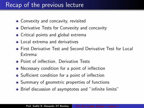
f (x)→∞ and f (x)→ −∞Definition

Let f : D → R and c ∈ R be such that there is r > 0 with(c − r , c) ∪ (c , c + r) ⊂ D. We say that f (x) tends to ∞ asx → c , and write f (x)→∞ as x → c if(xn) is a sequence in D, xn 6= c and xn → c =⇒ f (xn)→∞.

By restricting to sequences (xn) in D with xn < c for alln ∈ N, we can define f (x)→∞ as x → c−. Similarly, we candefine f (x)→∞ as x → c+, and furthermore, we can alsodefine f (x)→ −∞ as x → c (or as x → c− or as x → c+).

Note: As in the case of sequences, we shall not writelimx→c

f (x) =∞ when f (x)→∞ as x → c . Likewise, we shall

not write limx→c

f (x) = −∞ when f (x)→ −∞ as x → c .

Example: Let f (x) := 1/x for x ∈ R \ {0}. Then f (x)→∞as x → 0+ and f (x)→ −∞ as x → 0−.


Asymptotes

Let D ⊂ R, and let f : D → R. There are three possible typesof asymptotes: horizontal, oblique and vertical. They all implynearness of the curve y = f (x) to a straight line.

A straight line y = b is called a horizontal asymptoteof the curve y = f (x) if

limx→∞

f (x) = b or limx→−∞

f (x) = b.

A straight line y = ax + b, where a 6= 0, is called anoblique asymptote of the curve y = f (x) if

limx→∞

(f (x)− ax − b) = 0 or limx→−∞

(f (x)− ax − b) = 0.

A line x = a is called a vertical asymptote of the curvey = f (x) iff (x)→∞ as x → a−, or f (x)→ −∞ as x → a−, orf (x)→∞ as x → a+, or f (x)→ −∞ as x → a+.


Illustrations of asymptotes


Examples of asymptotesExample: Consider f : (−∞, 0) ∪ (1,∞)→ R defined by

f (x) :=

{(3x2 + 4x + 1)/x if x < 0,(2x − 1)/(x − 1) if x > 1.

For x > 1, we have f (x) = 2 + 1/(x − 1), and solimx→∞

f (x) = 2. Hence the straight line y = 2 is a

horizontal asymptote of the curve y = f (x).

For x < 0, f (x) = 3x + 4 + (1/x), and solim

x→−∞(f (x)− (3x + 4)) = 0. Hence the straight line

y = 3x + 4 is an oblique asymptote of the curve y = f (x).

f (x)→∞ as x → 1+. Hence the straight line x = 1 is avertical asymptote of the curve y = f (x).

f (x)→ −∞ as x → 0−. Hence the straight line x = 0 isa vertical asymptote of the curve y = f (x).

Exercise: Sketch the graph of f .Prof. Sudhir R. Ghorpade, IIT Bombay MA 105 Calculus: Division 1, Lecture 7

Even, odd and periodic functions

A function f : (−a, a)→ R is called even if f (−x) = f (x),and it is called odd if f (−x) = −f (x) for all x ∈ (−a, a).

If f : R→ R and f (x) = f (x + p) for a fixed p > 0 and allx ∈ R, then f is called periodic and p is called a period of f .


Curve Sketching: Tips

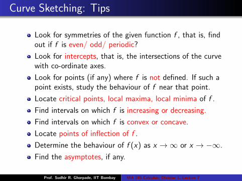
Look for symmetries of the given function f , that is, findout if f is even/ odd/ periodic?

Look for intercepts, that is, the intersections of the curvewith co-ordinate axes.

Look for points (if any) where f is not defined. If such apoint exists, study the behaviour of f near that point.

Locate critical points, local maxima, local minima of f .

Find intervals on which f is increasing or decreasing.

Find intervals on which f is convex or concave.

Locate points of inflection of f .

Determine the behaviour of f (x) as x →∞ or x → −∞.

Find the asymptotes, if any.


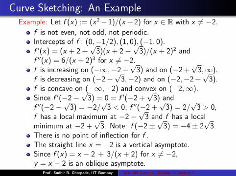
Curve Sketching: An ExampleExample: Let f (x) := (x2−1)/(x + 2) for x ∈ R with x 6= −2.

f is not even, not odd, not periodic.Intercepts of f : (0,−1/2), (1, 0), (−1, 0).f ′(x) = (x + 2 +

√3)(x + 2−

√3)/(x + 2)2 and

f ′′(x) = 6/(x + 2)3 for x 6= −2.f is increasing on (−∞,−2−

√3) and on (−2 +

√3,∞).

f is decreasing on (−2−√

3,−2) and on (−2,−2 +√

3).f is concave on (−∞,−2) and convex on (−2,∞).Since f ′(−2−

√3) = 0 = f ′(−2 +

√3) and

f ′′(−2−√

3) = −2/√

3 < 0, f ′′(−2 +√

3) = 2/√

3 > 0,f has a local maximum at −2−

√3 and f has a local

minimum at −2 +√

3. Note: f (−2±√

3) = −4± 2√

3.There is no point of inflection for f .The straight line x = −2 is a vertical asymptote.Since f (x) = x − 2 + 3/(x + 2) for x 6= −2,y = x − 2 is an oblique asymptote.


Mean Value Theorem Revisited

Recall the most important result in differential calculus whichwe proved in Lecture 7:

Theorem (Mean Value Theorem: MVT)

Let a < b and let f : [a, b]→ R be continuous on [a, b] anddifferentiable on (a, b). Then there exists c ∈ (a, b) such that

f (b) = f (a) + f ′(c)(b − a).

Let us now consider an extension of the above result.

Theorem (Extended Mean Value Theorem)

Let a < b and f : [a, b]→ R be such that f ′ exists on [a, b].Suppose f ′ is continuous on [a, b] and differentiable on (a, b).Then there exists c ∈ (a, b) such that

f (b) = f (a) + f ′(a)(b − a) +f ′′(c)

2(b − a)2.


Proof: For x ∈ [a, b], let P(x) := f (a) + f ′(a)(x − a). Define

F (x) := f (x)− P(x)− f (b)− P(b)

(b − a)2(x − a)2 for x ∈ [a, b].

Then F (a) = 0 = F (b). By the Rolle theorem, there existsc1 ∈ (a, b) such that F ′(c1) = 0. Since F ′(a) = 0 also, there isc ∈ (a, c1) such that F ′′(c) = 0. This gives the desired result.

More generally, we can obtain the following important result.

Theorem (Taylor Theorem)

Let a < b and n ∈ N. Let f : [a, b]→ R be such thatf ′, . . . , f (n) exist on [a, b]. Suppose f (n) is continuous on [a, b]and differentiable on (a, b). Then there exists c ∈ (a, b) such

that f (b) = f (a) + f ′(a)(b − a) + · · ·+ f (n)(a)

n!(b − a)n + Rn

where Rn := f (n+1)(c)(b − a)n+1/(n + 1)!.


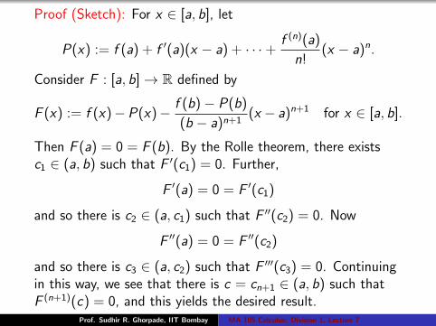
Proof (Sketch): For x ∈ [a, b], let

P(x) := f (a) + f ′(a)(x − a) + · · ·+ f (n)(a)

n!(x − a)n.

Consider F : [a, b]→ R defined by

F (x) := f (x)−P(x)− f (b)− P(b)

(b − a)n+1(x − a)n+1 for x ∈ [a, b].

Then F (a) = 0 = F (b). By the Rolle theorem, there existsc1 ∈ (a, b) such that F ′(c1) = 0. Further,

F ′(a) = 0 = F ′(c1)

and so there is c2 ∈ (a, c1) such that F ′′(c2) = 0. Now

F ′′(a) = 0 = F ′′(c2)

and so there is c3 ∈ (a, c2) such that F ′′′(c3) = 0. Continuingin this way, we see that there is c = cn+1 ∈ (a, b) such thatF (n+1)(c) = 0, and this yields the desired result.


A result similar to Taylor’s theorem holds with a and binterchanged. [This can be seen by applying Taylor’s Theoremto g : [a, b]→ R defined by g(x) := f (a + b − x).] As aconsequence, we obtain the following result.

Taylor Formula: Let n ∈ N. If I is an interval, a ∈ I , andf : I → R is such that f ′, f ′′, . . . , f (n) exist on I and f (n+1)

exists at every interior point of I , then for x ∈ I , x 6= a, thereis cx between a and x such that f (x) = Pn(x) + Rn(x), where

Pn(x) := f (a) + f ′(a)(x − a) + · · ·+ f (n)(a)

n!(x − a)n,

Rn(x) :=f (n+1)(cx)

(n + 1)!(x − a)n+1.

Here the polynomial Pn(x) is of degree ≤ n, and it can beconsidered as an ‘approximation’ of f (x) of order n. It iscalled the nth Taylor polynomial of f around a, and Rn(x) iscalled the nth Lagrange remainder of f around a.


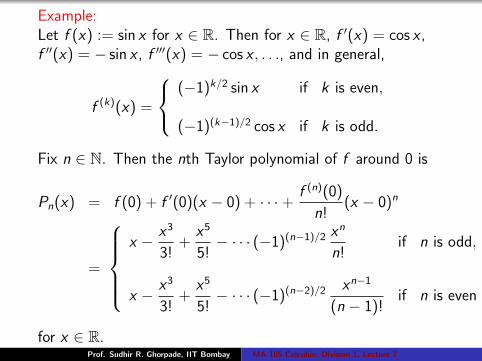
Example:Let f (x) := sin x for x ∈ R. Then for x ∈ R, f ′(x) = cos x ,f ′′(x) = − sin x , f ′′′(x) = − cos x , . . ., and in general,

f (k)(x) =

(−1)k/2 sin x if k is even,

(−1)(k−1)/2 cos x if k is odd.

Fix n ∈ N. Then the nth Taylor polynomial of f around 0 is

Pn(x) = f (0) + f ′(0)(x − 0) + · · ·+ f (n)(0)

n!(x − 0)n

=

x − x3

3!+

x5

5!− · · · (−1)(n−1)/2

xn

n!if n is odd,

x − x3

3!+

x5

5!− · · · (−1)(n−2)/2

xn−1

(n − 1)!if n is even

for x ∈ R.Prof. Sudhir R. Ghorpade, IIT Bombay MA 105 Calculus: Division 1, Lecture 7

Let x ∈ R. Then the nth Lagrange remainder around 0 is

Rn(x) =

(−1)n/2

xn+1

(n + 1)!cos cx if n is even,

(−1)(n+1)/2 xn+1

(n + 1)!sin cx if n is odd,

where cx is between 0 and x . As | cos cx | ≤ 1 & | sin cx | ≤ 1,

|Rn(x)| ≤ |x |n+1

(n + 1)!→ 0 as n→∞.

Hence for x ∈ R,

sin x = limn→∞

Pn(x) = limn→∞

n∑k=1

(−1)(k−1)x2k−1

(2k − 1)!, that is,

sin x =∞∑k=1

(−1)(k−1)x2k−1

(2k − 1)!= x − x3

3!+

x5

5!− x7

7!+ · · · .

The RHS is the Taylor series of the function sin around 0.Prof. Sudhir R. Ghorpade, IIT Bombay MA 105 Calculus: Division 1, Lecture 7

Riemann Integration

Let a, b ∈ R with a < b, and let f be a bounded functiondefined on [a, b]. Let us first assume that f ≥ 0 on [a, b].We are interested in assigning a meaning to the concept of‘area’ of the region that lies under the graph of f , between thelines x = a, x = b, and above the x-axis, that is, of the region

Rf := {(x , y) ∈ R2 : a ≤ x ≤ b and 0 ≤ y ≤ f (x)}.

A partition of [a, b] is a finite ordered setP := {x0, x1, . . . , xn} of points in [a, b] such thata = x0 < x1 < x2 < · · · < xn = b, where n ∈ N.

The points in a partition divide the interval [a, b] intononoverlapping subintervals, [x0, x1], . . . , [xn−1, xn]. We call[xi−1, xi ] the ith subinterval of the partition P .


Example: For n ∈ N, the set

Pn :=

{a, a +

(b − a)

n, . . . , a +

(n − 1)(b − a)

n, b

}is a partition of [a, b] into n equal parts, each of length(b − a)/n. If n := 1, then P1 := {a, b} is the trivial partition.

Let f : [a, b]→ R be any bounded function, and define

m(f ) := inf{f (x) : x ∈ [a, b]} and M(f ) := sup{f (x) : x ∈ [a, b]}.

Given a partition P := {x0, x1, . . . , xn} of [a, b], let us define

mi(f ) := inf{f (x) : x ∈ [xi−1, xi ]}

andMi(f ) := sup{f (x) : x ∈ [xi−1, xi ]}

for i = 1, . . . , n.Prof. Sudhir R. Ghorpade, IIT Bombay MA 105 Calculus: Division 1, Lecture 7

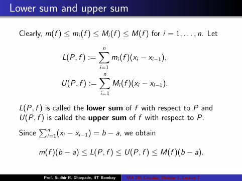
Lower sum and upper sum

Clearly, m(f ) ≤ mi(f ) ≤ Mi(f ) ≤ M(f ) for i = 1, . . . , n. Let

L(P , f ) :=n∑

i=1

mi(f )(xi − xi−1),

U(P , f ) :=n∑

i=1

Mi(f )(xi − xi−1).

L(P , f ) is called the lower sum of f with respect to P andU(P , f ) is called the upper sum of f with respect to P .

Since∑n

i=1(xi − xi−1) = b − a, we obtain

m(f )(b − a) ≤ L(P , f ) ≤ U(P , f ) ≤ M(f )(b − a).


Underlying assumption: The area of a rectangle[xi−1, xi ]× [yi−1, yi ] is equal to (xi − xi−1)(yi − yi−1).

x

y

a xi−1 xi bx

y

a xi−1 xi b

Figure: Approximating the ‘area’ under a curve by a lower sumwhich is sum of the areas of the inscribed rectangles, and by anupper sum which is the sum of the areas of the circumscribingrectangles.


MA 105 : Calculus Division 1, Lecture 7

Documents

Transcript of MA 105 : Calculus Division 1, Lecture 7