M4 Macros for Electric Circuit Diagrams in LATEX Documents

Dwight Aplevich

Version 5.97

Contents

1 Introduction . . . . . . . . . . . . . . . . . . . . . . . . . . . . . . . . . . . . . . . . . . . . . . . . . . . . . . . . . . . . . . . . . 2

2 Using the macros . . . . . . . . . . . . . . . . . . . . . . . . . . . . . . . . . . . . . . . . . . . . . . . . . . . . . . . . . . . . 22.1 Quick start . . . . . . . . . . . . . . . . . . . . . . . . . . . . . . . . . . . . . . . . . 2

2.1.1 Processing with gpic . . . . . . . . . . . . . . . . . . . . . . . . . . . . . . . . 32.1.2 Processing with dpic and PSTricks or Tikz PGF . . . . . . . . . . . . . . . 32.1.3 Simplifications . . . . . . . . . . . . . . . . . . . . . . . . . . . . . . . . . . . 4

3 Pic essentials . . . . . . . . . . . . . . . . . . . . . . . . . . . . . . . . . . . . . . . . . . . . . . . . . . . . . . . . . . . . . . . . 43.1 Manuals . . . . . . . . . . . . . . . . . . . . . . . . . . . . . . . . . . . . . . . . . . . 53.2 The linear objects: line, arrow, spline, arc . . . . . . . . . . . . . . . . . . . . 53.3 The planar objects: box, circle, ellipse, and text . . . . . . . . . . . . . . . . . 63.4 Compound objects . . . . . . . . . . . . . . . . . . . . . . . . . . . . . . . . . . . . . 73.5 Other language elements . . . . . . . . . . . . . . . . . . . . . . . . . . . . . . . . . . 7

4 Two-terminal elements . . . . . . . . . . . . . . . . . . . . . . . . . . . . . . . . . . . . . . . . . . . . . . . . . . . . . . 74.1 Circuit and element basics . . . . . . . . . . . . . . . . . . . . . . . . . . . . . . . . . 84.2 The two-terminal elements . . . . . . . . . . . . . . . . . . . . . . . . . . . . . . . . . 94.3 Branch-current arrows . . . . . . . . . . . . . . . . . . . . . . . . . . . . . . . . . . . 124.4 Labels . . . . . . . . . . . . . . . . . . . . . . . . . . . . . . . . . . . . . . . . . . . . 12

5 Other circuit elements . . . . . . . . . . . . . . . . . . . . . . . . . . . . . . . . . . . . . . . . . . . . . . . . . . . . . . . 13

6 Directions and macro-level looping . . . . . . . . . . . . . . . . . . . . . . . . . . . . . . . . . . . . . . . . . . . 18

7 Logic gates . . . . . . . . . . . . . . . . . . . . . . . . . . . . . . . . . . . . . . . . . . . . . . . . . . . . . . . . . . . . . . . . . . 19

8 Element and diagram scaling . . . . . . . . . . . . . . . . . . . . . . . . . . . . . . . . . . . . . . . . . . . . . . . . 228.1 Circuit scaling . . . . . . . . . . . . . . . . . . . . . . . . . . . . . . . . . . . . . . . 228.2 Pic scaling . . . . . . . . . . . . . . . . . . . . . . . . . . . . . . . . . . . . . . . . . . 22

9 Writing macros . . . . . . . . . . . . . . . . . . . . . . . . . . . . . . . . . . . . . . . . . . . . . . . . . . . . . . . . . . . . . . 23

10 Interaction with LATEX . . . . . . . . . . . . . . . . . . . . . . . . . . . . . . . . . . . . . . . . . . . . . . . . . . . . . . . 24

11 PSTricks tricks . . . . . . . . . . . . . . . . . . . . . . . . . . . . . . . . . . . . . . . . . . . . . . . . . . . . . . . . . . . . . . 26

12 Web documents, pdf, and alternative output formats . . . . . . . . . . . . . . . . . . . . . . . . . 26

13 Developer’s notes . . . . . . . . . . . . . . . . . . . . . . . . . . . . . . . . . . . . . . . . . . . . . . . . . . . . . . . . . . . . 27

14 Bugs . . . . . . . . . . . . . . . . . . . . . . . . . . . . . . . . . . . . . . . . . . . . . . . . . . . . . . . . . . . . . . . . . . . . . . . . 28

15 List of macros . . . . . . . . . . . . . . . . . . . . . . . . . . . . . . . . . . . . . . . . . . . . . . . . . . . . . . . . . . . . . . . 30

1

1 Introduction

Before every conference, I find Ph.D.s in on weekends running back and forth fromtheir offices to the printer. It appears that people who are unable to execute prettypictures with pen and paper find it gratifying to try with a computer [9].

This document describes a set of macros, written in the m4 macro language [7], for producingelectric circuits and other diagrams in LATEX documents. The macros evaluate to drawing commandsin pic, a line-drawing language [8] that is readily available and quite simple to learn. The resultis a system with the advantages and disadvantages of TEX itself, since it is macro-based and non-wysiwyg, and since it uses ordinary character input. The book from which the above quotation istaken correctly points out that the payoff can be in quality of diagrams at the price of the timespent in learning how to draw them.

A collection of basic components and conventions for their internal structure are described. Forparticular drawings it is often convenient to customize elements or to package combinations of them,so macros such as these are only a starting point. The IEEE standard [6] has been followed mostof the time. The macros described here make extensive use of the characteristics of pic and havebeen designed, where possible, to be an extension of the language.

2 Using the macros

The diagram source file is preprocessed as illustrated in Figure 1. The predefined macros, followedby the diagram source, are read by m4. The result is passed through a pic interpreter to produce.tex output that can be inserted into a .tex document using the \input command.

.m4diagram

.m4macros

m4pic

interpreter

.texfiles

LATEX .dvifile

Figure 1: Inclusion of figures and macros in the LATEX document. Replacing LATEX with PDFlatexto produce pdf directly is also possible.

Depending on the pic interpreter chosen and choice of options, the interpreter output may containtpic specials, LATEX graphics, PSTricks [14] commands, Tikz PGF commands, or other formats,which LATEX or PDFlatex will process. These variations are described in Section 12.

There are two principal choices of pic interpreter. One is [3] gpic -t together with a printerdriver that understands tpic specials, typically [11] dvips. In some installations, gpic is simplynamed pic, but make sure that GNU pic [3] is being invoked rather than the older Unix pic. Analternative is dpic, described later in this document. Pic processors contain basic macro facilities,so some of the concepts applied here require only a pic processor.

By judicious use of macros, features of both m4 and pic can be exploited. The fastidious readermight observe that there are three languages being scrambled: m4, pic, and the tpic, tex or otheroutput, not to mention the meta-language of the macros, and that this mixture might be a problem,but experience implies otherwise.

2.1 Quick start

The contents of file quick.m4 and resulting diagram are shown in Figure 2 to illustrate the language,to show several ways for placing circuit elements, and to provide information sufficient for producingbasic labeled circuits.

2

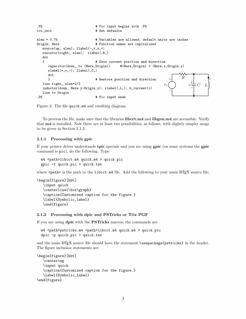
.PS # Pic input begins with .PS

cct_init # Set defaults

elen = 0.75 # Variables are allowed; default units are inches

Origin: Here # Position names are capitalized

source(up_ elen); llabel(-,v_s,+)

resistor(right_ elen); rlabel(,R,)

dot

{ # Save current position and direction

capacitor(down_ to (Here,Origin)) #(Here,Origin) = (Here.x,Origin.y)

rlabel(+,v,-); llabel(,C,)

dot

} # Restore position and direction

line right_ elen*2/3

inductor(down_ Here.y-Origin.y); rlabel(,L,); b_current(i)

line to Origin

.PE # Pic input ends

−vs

+ R+

v− C L

i

Figure 2: The file quick.m4 and resulting diagram.

To process the file, make sure that the libraries libcct.m4 and libgen.m4 are accessible. Verifythat m4 is installed. Now there are at least two possibilities, as follows, with slightly simpler usageto be given in Section 2.1.3.

2.1.1 Processing with gpic

If your printer driver understands tpic specials and you are using gpic (on some systems the gpiccommand is pic), do the following. Type

m4 <path>libcct.m4 quick.m4 > quick.picgpic -t quick.pic > quick.tex

where <path> is the path to the libcct.m4 file. Add the following to your main LATEX source file:

\begin{figure}[hbt]\input quick\centerline{\box\graph}\caption{Customized caption for the figure.}\label{Symbolic_label}\end{figure}

2.1.2 Processing with dpic and PSTricks or Tikz PGF

If you are using dpic with the PSTricks macros, the commands are

m4 <path>pstricks.m4 <path>libcct.m4 quick.m4 > quick.picdpic -p quick.pic > quick.tex

and the main LATEX source file should have the statement \usepackage{pstricks} in the header.The figure inclusion statements are

\begin{figure}[hbt]\centering\input quick\caption{Customized caption for the figure.}\label{Symbolic_label}

\end{figure}

3

This distribution is compatible with the Tikz PGF drawing commands, which have nearly the powerof the PSTricks package with the ability to produce pdf output by running the pdflatex commandinstead of latex on the input file. The commands are modified to read pgf.m4 and invoke the -gdpic option as follows:

m4 <path>pgf.m4 <path>libcct.m4 quick.m4 > quick.picdpic -g quick.pic > quick.tex

The header should contain \usepackage{tikz}, but the inclusion statemensts are the same as forPSTricks input.

In all cases the essential line is \input quick, which inserts the previously created file quick.tex.Then LATEX the document, convert to postscript typically using dvips, and print the result or viewit using Ghostview. The alternative for Tikz PGF output of dpic -g is to invoke PDFlatex.

2.1.3 Simplifications

If appropriate include() statements are placed at the top of the file quick.m4, then the m4commands illustrated above can be shortened to

m4 quick.m4 > quick.picFor example, the following two lines can be inserted before the line containing .PS:

include(<path>pstricks.m4)include(<path>libcct.m4)

where <path> is the path to the folder containing the libraries. Only the second line is necessaryif gpic is used or if the libraries were installed so that PSTricks is assumed by default. On somesystems, setting the environment variable M4PATH to the library folder allows the above lines to besimplified to

include(pstricks.m4)include(libcct.m4)In the absence of a need to examine the file quick.pic, the commands for producing the .tex

file can be reduced tom4 quick.m4 | dpic -p > quick.texWhen many files are to be processed, then a facility such as Unix make, which is also available

in several PC versions, can be employed to automate the manual commands given above. Onsystems without such a facility, a scripting language can be used. Alternatively, you can put severaldiagrams into a single source file so that they can be processed together, as follows. Put eachdiagram in the body of a LATEX macro, as shown:

\newcommand{\diaA}{%.PSdrawing commands.PE\box\graph }% \box\graph not required for dpic\newcommand{\diaB}{%.PSdrawing commands.PE\box\graph }% \box\graph not required for dpicProcess the file using m4 and dpic or gpic to produce a .tex file, insert this into the LATEX

source using \input, and invoke the macros at the appropriate places.

3 Pic essentials

Pic source is a sequence of lines in a file. The first line of a diagram begins with .PS with optionalfollowing arguments, and the last line is normally .PE. Lines outside of these pass through the picprocessor unchanged.

The visible objects can be divided conveniently into two classes, the linear objects line, arrow,spline, arc, and the planar objects box, circle, ellipse.

4

The object move is linear but draws nothing. A composite object, or block, is planar andconsists of a pair of square brackets enclosing other objects, as described in Section 3.4. Objectscan be placed using absolute coordinates or relative to other objects.

Pic allows the definition of real-valued variables, which are alphameric names beginning withlower-case letters, and computations using them. Objects or locations on the diagram can be givensymbolic names beginning with an upper-case first letter.

3.1 Manuals

At the time of writing, the classic pic manual [8] can be obtained from URL:http://www.cs.bell-labs.com/10thEdMan/pic.pdfA more complete manual [10] is included in the GNU groff package. A compressed postscript

versions is available, at least temporarily, with these circuit files.In both of the above manuals, explicit use of *roff string and font constructs should be replaced

by their LATEX equivalents as necessary. Further explanation is available, for example, from thegpic ‘man’ page, part of the GNU groff package.

Examples of use of the circuit macros in an electronics course are available on the web [2].For a discussion of “little languages” for document production, and of pic in particular, see

Chapter 9 of [1]. Chapter 1 of [4] also contains a brief discussion of this and other languages.

3.2 The linear objects: line, arrow, spline, arc

A line can be drawn as follows:line from position to position

where position is defined below orline direction distance

where direction is one of up, down, left, right. When used with the m4 macros described here,it is preferable to add an underscore: up , down , left , right . The distance is a number orexpression and the units are inches, but the assignment

scale = 25.4has the effect of changing the units to millimetres, as described in Section 8.

Lines can also be drawn to any distance in any direction. The example,line up 3/sqrt(2) right 3/sqrt(2)

draws a line 3 units long from the current location, at a 45◦ angle above horizontal.The constructionline from A to B chop x

truncates the line at each end by x or, if x is omitted, by the current circle radius, which is convenentwhen A and B are symbolic names for circular graph nodes, for example. Otherwise

line from A to B chop x chop ytruncates the line ends by x and and y, which may be negative.

The above methods of specifying the direction and length of a line are referred to as a linespec.Lines can be concatenated. For example, to draw a triangle:line up sqrt(3) right 1 then down sqrt(3) right 1 then left 2A position can be defined by a coordinate pair, e.g. 3,2.5, more generally using parentheses

by (expression, expression), or by the construction (position, position), the latter taking the x-coordinate from the first position and the y-coordinate from the second. A position can be givena symbolic name beginning with an upper-case letter, e.g. Top: (0.5,4.5). Such a definitiondoes not affect the calculated figure boundaries. The current position Here is always defined. Thecoordinates of a position are accessible, e.g. Top.x and Top.y can be used in expressions. Thecenter, start, and end of linear objects are valid positions, as shown in the following example, whichalso illustrates how to refer to a previously-drawn element if it has not been given a name:

line from last line.start to 2nd last arrow.end then to 3rd line.centerObjects can be named (using a name commencing with an upper-case letter), for example:Bus23: line up right

after which, positions associated with the object can be referenced using the name; for example:

5

arc cw from Bus23.start to Bus23.end with .center at Bus23.centerAn arc is drawn by specifying its rotation, starting point, end point, and center, but sensible

defaults are assumed if any of these are omitted. Note thatarc cw from Bus23.start to Bus23.end

does not define the arc uniquely; there are two arcs that satisfy this specification. This distributionincludes the m4 macros

arcr( position, radius, start radians, end radians)arcd( position, radius, start degrees, end degrees)arca( chord linespec, ccw|cw, radius, modifiers)

to draw uniquely defined arcs. For example,arcd((1,1),2,0,-90) -> dashed cw

draws a clockwise arc with centre at (1, 1), radius 2, from (3, 1) to (1,−1), andarca(from (1,1) to (2,2),,1,->)

draws an acute-angled arc with arrowhead on the chord defined by the first argument.The linear objects can be given arrowheads at the start, end, or both ends, for example:line dashed <- right 0.5arc <-> height 0.06 width 0.03 ccw from Here to Here+(0.5,0) \

with .center at Here+(0.25,0)spline -> right 0.5 then down 0.2 left 0.3 then right 0.4The arrowheads on the arc above have had their shape adjusted using the height and width

parameters.Finally, lines can be specified as dotted, dashed, or invisible, as in the above example.

3.3 The planar objects: box, circle, ellipse, and text

The planar objects are drawn by specifying the width, height, and center position, thus:A: box ht 0.6 wid 0.8 at (1,1)

after which, in this example, the position A.center is defined, and can be referenced simply as A.In addition, the compass corners A.n, A.s, A.e, A.w, A.ne, A.se, A.sw, A.nw are automaticallydefined, as are the dimensions A.height and A.width. For example, two touching circles can bedrawn as shown:

circle radius 0.2circle diameter (last circle.width * 1.2) with .sw at last circle.neThe planar objects can be filled with gray or colour; thusbox dashed fill

produces a dashed box filled with a medium gray by default. The gray density can be controlledusing the fill_(number) macro, where 0 ≤ number ≤ 1, with 0 and 1 meaning respectively blackand white.

Basic colours for lines and fills are provided by gpic and dpic, but more elaborate line and fillstyles can be incorporated, depending on the printing device, by inserting \special commands orother lines beginning with a backslash in the drawing code. In fact, arbitrary lines can be insertedinto the output using

command "string"where string is the line to be inserted.

Arbitrary text strings, typically meant to be typeset by LATEX, are delimited by double-quotecharacters and occur in two ways. The first way is illustrated by

"\large Resonances of $C_{20}H_{42}$" wid x ht y at positionwhich writes the typeset result, like a box, at position and tells pic its size. The default size assumedby pic is given by parameters textwid and textht if it is not specified as above. The exact typesetsize of formatted text can be obtained as described in Section 10. The second way of occurrenceassociates strings with an object, e.g., the following writes two words, one above the other, at thecentre of an ellipse:

ellipse "\bf Stop" "\bf here"The C-like pic function sprintf("format string",numerical arguments) is equivalent to a string.

6

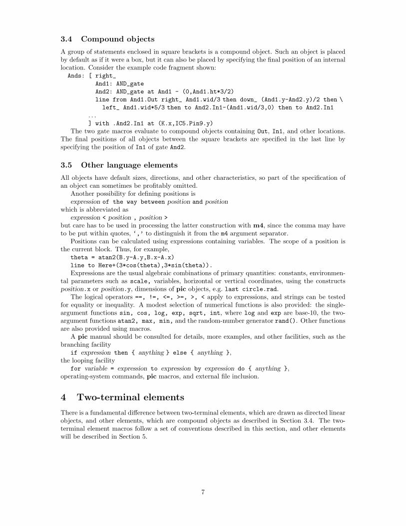
3.4 Compound objects

A group of statements enclosed in square brackets is a compound object. Such an object is placedby default as if it were a box, but it can also be placed by specifying the final position of an internallocation. Consider the example code fragment shown:Ands: [ right_

And1: AND_gateAnd2: AND_gate at And1 - (0,And1.ht*3/2)line from And1.Out right_ And1.wid/3 then down_ (And1.y-And2.y)/2 then \left_ And1.wid*5/3 then to And2.In1-(And1.wid/3,0) then to And2.In1

. . .] with .And2.In1 at (K.x,IC5.Pin9.y)

The two gate macros evaluate to compound objects containing Out, In1, and other locations.The final positions of all objects between the square brackets are specified in the last line byspecifying the position of In1 of gate And2.

3.5 Other language elements

All objects have default sizes, directions, and other characteristics, so part of the specification ofan object can sometimes be profitably omitted.

Another possibility for defining positions isexpression of the way between position and position

which is abbreviated asexpression < position , position >

but care has to be used in processing the latter construction with m4, since the comma may haveto be put within quotes, ‘,’ to distinguish it from the m4 argument separator.

Positions can be calculated using expressions containing variables. The scope of a position isthe current block. Thus, for example,

theta = atan2(B.y-A.y,B.x-A.x)line to Here+(3*cos(theta),3*sin(theta)).Expressions are the usual algebraic combinations of primary quantities: constants, environmen-

tal parameters such as scale, variables, horizontal or vertical coordinates, using the constructsposition.x or position.y, dimensions of pic objects, e.g. last circle.rad.

The logical operators ==, !=, <=, >=, >, < apply to expressions, and strings can be testedfor equality or inequality. A modest selection of numerical functions is also provided: the single-argument functions sin, cos, log, exp, sqrt, int, where log and exp are base-10, the two-argument functions atan2, max, min, and the random-number generator rand(). Other functionsare also provided using macros.

A pic manual should be consulted for details, more examples, and other facilities, such as thebranching facility

if expression then { anything } else { anything },the looping facility

for variable = expression to expression by expression do { anything },operating-system commands, pic macros, and external file inclusion.

4 Two-terminal elements

There is a fundamental difference between two-terminal elements, which are drawn as directed linearobjects, and other elements, which are compound objects as described in Section 3.4. The two-terminal element macros follow a set of conventions described in this section, and other elementswill be described in Section 5.

7

4.1 Circuit and element basics

First, the arguments of all drawing macros have default values, so that only arguments that differfrom these values need be specified. The arguments are given in Section 15.

Consider the resistor shown in Figure 3, which also serves as an example of pic command; thefirst part of the source is as follows:

.PS

cct_init

linewid = 2.0

linethick_(2.0)

R1: resistor

last []R1.start R1.endR1.centre

elendimen

Figure 3: Resistor named R1, showing the size parameters, enclosing block, and predefined positions.

The lines of Figure 3 and the remaining source lines of the file are explained below:

• The first line invokes an almost-empty macro that initializes local variables needed by somecircuit-element macros. This macro can be customized to set line thicknesses, maximum pagesizes, scale parameters, or other global quantities as desired.

• The body dimensions of two-terminal elements are multiples of the macro dimen , whichevaluates by default to linewid, the pic environment variable with default value 0.5 in. Thedefault length of an element is elen , which is dimen *3/2. For resistors, the length of thebody is dimen /2, and the width is dimen /6. All of these values can be customized. Elementscaling is discussed further in Section 8.

• The macro linethick sets the thickness of subsequent lines (to 2.0 pt in the example).

• The two-terminal element macros expand to sequences of drawing commands that begin with‘line invis linespec’, where linespec is the first argument of the macro if it is non-blank,otherwise by default the line is drawn a distance elen in the current direction, which is tothe right by default. The invisible line is first drawn, then the element is drawn on top of theline. The element—rather the initially-drawn invisible line—can be given a name, R1 in theexample, so that positions R1.start, R1.centre, and R1.end are defined as shown.

• The element body is enclosed by a block, which later can be used to place labels aroundthe element. The block corresponds to an invisible rectangle with horizontal top and bottomlines, regardless of the direction in which the element is drawn. In the diagram a dotted boxhas been drawn to show the block boundaries.

• The last sub-element, identical to the first in each two-terminal element, is an invisible linethat can be referenced later to place labels or other elements. This might be over-kill. If youcreate your own macros you might choose simplicity over generality, and only include visiblelines.

To produce Figure 3, the following embellishments were included after the previously-shownsource:

thinlines_

box dotted wid last [].wid ht last [].ht at last []

8

move to 0.85<last [].sw,last [].se>

spline <- down arrowht*2 right arrowht/2 then right 0.15; "\tt last []" ljust

arrow <- down 0.3 from R1.start chop 0.05; "\tt R1.start" below

arrow <- down 0.3 from R1.end chop 0.05; "\tt R1.end" below

arrow <- down last [].c.y-last arrow.end.y from R1.c; "\tt R1.centre" below

dimension_(from R1.start to R1.end,0.45,\tt elen\_,0.4)

dimension_(right_ dimen_ from R1.c-(dimen_/2,0),0.3,\tt dimen\_,0.5)

.PE

• The line thickness is set to the default thin value of 0.4pt, and the box displaying the elementbody block is drawn. Notice how the width and height can be specified, and the box centrepositioned at the centre of the block.

• The next paragraph draws two objects, a spline with an arrowhead, and a string left justifiedat the end of the spline. Other string-positioning modifiers than ljust are rjust, above,and below. Lines to be read by pic can be continued by putting a backslash as the rightmostcharacter.

• The last paragraph invokes a macro for dimensioning diagrams.

4.2 The two-terminal elements

Figures 4–9 are tables of the two-terminal elements. Several elements are included more than onceto illustrate some of their arguments, which are listed in Section 15. In the m4 language, macroarguments are written within parentheses following the macro name, with no space between thename and the opening parenthesis. Lines can be broken before a macro argument because m4ignores white space before arguments.

The first argument of the two-terminal elements, if included, defines the invisible line alongwhich the element is drawn. The other arguments produce variants of the default elements. Thus,for example,

resistor(up 1.25,7)draws a resistor 1.25 units long up from the current position, with 7 vertices per side. The macroup evaluates to up but also resets the current directional parameters to point up.

resistor

resistor(,E) ≡ ebox

resistor(,,Q)

resistor(,,H)

resistor(,4,QR)

inductor

inductor(,W)

inductor(,,,M)

inductor(,W,6,M)

arrowline

capacitor

capacitor(,C)

capacitor(,E)

capacitor(,K)

xtal

tline

gap

gap(,,A)

ebox(,0.5,0.3)

ebox(,,,0.5)

Figure 4: Two-terminal elements, showing some variations.

9

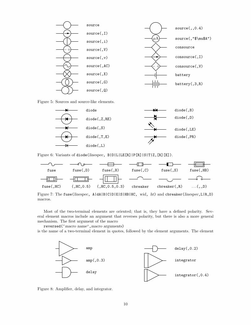
source

source(,I)

source(,i)

−+ source(,V)

source(,v)

source(,AC)

source(,X)

source(,G)

source(,Q)

source(,,0.4)

μA source(,"$\mu$A")

consource

consource(,I)

− + consource(,V)

battery

battery(,3,R)

Figure 5: Sources and source-like elements.

diode

diode(,Z,RE)

diode(,S)

diode(,T,E)

diode(,L)

diode(,B)

diode(,D)

diode(,LE)

diode(,PR)

Figure 6: Variants of diode(linespec, B|D|L|LE[R]|P[R]|S|T|Z,[R][E]).

fuse fuse(,D) fuse(,B) fuse(,C) fuse(,S) fuse(,HB)

fuse(,HC) (,HC,0.5) (,HC,0.5,0.3) cbreaker cbreaker(,R) . . .(,,D)

Figure 7: The fuse(linespec, A|dA|B|C|D|E|S|HB|HC, wid, ht) and cbreaker(linespec,L|R,D)macros.

Most of the two-terminal elements are oriented; that is, they have a defined polarity. Sev-eral element macros include an argument that reverses polarity, but there is also a more generalmechanism. The first argument of the macro

reversed(‘macro name’,macro arguments)is the name of a two-terminal element in quotes, followed by the element arguments. The element

amp

amp(,0.3)

delay

delay(,0.2)

integrator

integrator(,0.4)

Figure 8: Amplifier, delay, and integrator.

10

switch (,,D) (,,OD) (,,C) (,,,B) (,,C,B)

dswitch=switch(,,,D)

W B

(,,WdBK)

dB K

(,,WBD) (,,WBF)(,,WdBKF)

(,,WBL)

(,,WdBKL)(,,WBT)

(,,WdBKC)(,,WBM) (,,WBCO) (,,WBMP)

(,,WBCY) (,,WBCZ) (,,WBCE) (,,WBRH) (,,WBRdH) (,,WBRHH)

(,,WBMMR) (,,WBMM) (,,WBMR) (,,WBEL) (,,WBLE)(,,WdBKEL)

Figure 9: The basic switch(linespec,L|R,[O|C][D],B) and more elabouratedswitch(linespec,R,W[ud]B[K]chars) macros, with drawing direction right . Setting thesecond argument to R produces a mirror image with respect to the drawing direction. The macroswitch(,,,D) is a wrapper for the comprehensive dswitch macro.

C S

A

P

L

N

Figure 10: Illustrating variable(‘element’,[A|P|L|[u]N][C|S],angle,length). For example,variable(‘capacitor(down dimen )’) draws the leftmost capacitor shown above, andvariable(‘resistor(down dimen )’,uN) draws the resistor. The default angle is 45◦, regardlessof the direction of the element. The array on the right shows the effect of the second argument.

is drawn with reversed direction. Thus,diode(right 0.4); reversed(‘diode’,right 0.4)

draws two diodes to the right, but the second one points left.Figure 10 shows some two-terminal elements with arrows or lines overlaid to indicate variability

using the macro variable(‘element’,type,angle,length), where type is one of A, P, L, N, withC or S optionally appended to indicate continuous or stepwise variation. Alternatively, this macrocan be invoked similarly to the label macros in section 4.4 by specifying an empty first argument;thus

resistor(down dimen ); variable(,uN)draws the resistor in Figure 10.

Figure 11 contains arrows for indicating radiation effects. The arrow stems are named A1, A2,and each pair is drawn in a [ ] block, with the names Head and Tail defined to aid placement nearanother device. The second argument specifies absolute angle in degrees (default 135 degrees).

11

Head

Tail

A1

A2

em arrows(N)

em arrows(ND,45) . . .(I) . . .(ID) . . .(E) . . .(ED)

Figure 11: Radiation arrows: em arrows(type, angle, length)

4.3 Branch-current arrows

Arrowheads and labels can be added to conductors using basic pic statements. For example, thefollowing line adds a labeled arrowhead at a distance alpha along a horizontal line that has justbeen drawn. Many variations of this are possible:

arrow right arrowht from last line.start+(alpha,0) "$i_1$" aboveMacros have been defined to simplify the labelling of two-terminal elements. The macrob current(label, above |below , In|O[ut], Start|E[nd], frac)

draws an arrow from the start of the last-drawn two-terminal element frac of the way toward thebody. If the fourth argument is End, the arrow is drawn from the end toward the body. If thethird element is Out, the arrow is drawn outward from the body. The first argument is the desiredlabel, of which the default position is the macro above , which evaluates to above if the currentdirection is right or to ljust, below, rjust if the current direction is respectively down, left, up.The label is assumed to be in math mode unless it begins with sprintf or a double quote, in whichcase it is copied literally. A non-blank second argument specifies the relative position of the labelwith respect to the arrow, for example below , which places the label below with respect to thecurrent direction. Absolute positions, for example below or ljust, also can be specified. Figure 12illustrates the resulting eight possibilities.

i

b current(i)i

. . .(i,below )

i

. . .(i,,O)i

. . .(i,below ,O)

i

b current(i,,,E)i

. . .(i,below ,,E)

i

. . .(i,,O,E,0.2)i

. . .(i,below ,O,E)

Figure 12: Illustrating b current. In all cases the drawing direction is to the right.

For those who prefer a separate arrow to indicate the reference direction for current, the macroslarrow(label, ->|<-,dist) and rarrow(label, ->|<-,dist) are provided. The label is placed out-side the arrow as shown in Figure 13. The first argument is assumed to be in math mode unless itbegins with sprintf or a double quote, in which case the argument is copied literally. The thirdargument specifies the separation from the element.

i

larrow(i)i

rarrow(i)

i

larrow(i,<-)i

rarrow(i,<-)

Figure 13: The larrow and rarrow macros are drawn adjacent to the element to provide a referencedirection.

4.4 Labels

Macros for labeling two-terminal elements are included:llabel( arg1,arg2,arg3 )clabel( arg1,arg2,arg3 )rlabel( arg1,arg2,arg3 )dlabel( long,lat,arg1,arg2,arg3 )

12

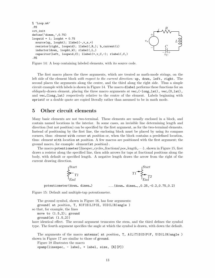
% ‘Loop.m4’

.PS

cct_init

define(‘dimen_’,0.75)

loopwid = 1; loopht = 0.75

source(up_ loopht); llabel(-,v_s,+)

resistor(right_ loopwid); llabel(,R,); b_current(i)

inductor(down_ loopht,W); rlabel(,L,)

capacitor(left_ loopwid,C); llabel(+,v_C,-); rlabel(,C,)

.PE

−vs

+

Ri

L

+vC

−C

Figure 14: A loop containing labeled elements, with its source code.

The first macro places the three arguments, which are treated as math-mode strings, on theleft side of the element block with respect to the current direction: up, down, left, right. Thesecond places the arguments along the centre, and the third along the right side. Thus a simplecircuit example with labels is shown in Figure 14. The macro dlabel performs these functions for anobliquely-drawn element, placing the three macro arguments at vec (-long,lat), vec (0,lat),and vec (long,lat) respectively relative to the centre of the element. Labels beginning withsprintf or a double quote are copied literally rather than assumed to be in math mode.

5 Other circuit elements

Many basic elements are not two-terminal. These elements are usually enclosed in a block, andcontain named locations in the interior. In some cases, an invisible line determining length anddirection (but not position) can be specified by the first argument, as for the two-terminal elements.Instead of positioning by the first line, the enclosing block must be placed by using its compasscorners, thus: element with corner at position or, when the block contains a predefined location,thus: element with location at position. A few macros are positioned with the first argument; theground macro, for example: element(at position).

The macro potentiometer(linespec,cycles,fractional pos,length,· · ·), shown in Figure 15, firstdraws a resistor along the specified line, then adds arrows for taps at fractional positions along thebody, with default or specified length. A negative length draws the arrow from the right of thecurrent drawing direction.

potentiometer(down dimen )

Start

End

T1

...(down dimen ,,0.25,-0.2,0.75,0.2)

Start

End

T1T2

Figure 15: Default and multiple-tap potentiometer.

The ground symbol, shown in Figure 16, has four arguments:ground( at position, T, N|F|S|L|P|E, U|D|L|R|angle )

so that, for example, the linesmove to (1.5,2); groundground(at (1.5,2))

have identical effect. The second argument truncates the stem, and the third defines the symboltype. The fourth argument specifies the angle at which the symbol is drawn, with down the default.

The arguments of the macro antenna( at position, T, A|L|T|S|D|P|F, U|D|L|R|angle )shown in Figure 17 are similar to those of ground.

Figure 18 illustrates the macroopamp(linespec, - label, + label, size, [R][P])

13

ground ground(,T) (,,F) (,,E) (,,S,90) (,,L) (,,P)

Figure 16: Ground symbols.

T

antenna

T

(,T)

T1 T2

(,,L)

T1 T2

(,T,L)

T

(,,T)

T1 T2

(,,S)

T1 T2

(,,D)

T

(,,P)

T

(,,F)

Figure 17: Antenna symbols, with macro arguments shown above and predefined terminal namesbelow.

−

+

opamp

Out

In1

In2

E1

E2

−

+

Point (15); opamp(,,,,PR)

V1

V2 − +

Point (90); opamp

Figure 18: Operational amplifiers. The P option adds power connections. The second and thirdarguments can be used to place and rotate arbitrary text at In1 and In2.

The element is enclosed in a block containing the predefined internal locations shown. Theselocations can be referenced in later commands, for example as ‘last [].Out.’ The first argumentdefines the direction and length of the opamp, but the position is determined either by the enclosingblock of the opamp, or by a construction such as ‘opamp with .In1 at Here’, which places theinternal position In1 at the specified location. There are optional second and third arguments forwhich the defaults are scriptsize$-$ and scriptsize$+$ respectively, and the fourth argumentchanges the size of the opamp. The fifth argument adds a power connection, exchanges the secondand third entries, or both.

Typeset text associated with circuit elements is not rotated by default, as illustrated by thesecond and third opamps in Figure 18. The opamp labels can be rotated if necessary by usingPSTricks \rput commands as second and third arguments, for example.

The code in Figure 19 places an opamp with three connections.

line right 0.2 then up 0.1

A: opamp(up_,,,0.4,R) with .In1 at Here

line right 0.2 from A.Out

line down 0.1 from A.In2 then right 0.2

−+

Figure 19: A code fragment invoking the opamp(linespec,-,+,size,[R][P]) macro.

Figure 20 shows variants of the transformer macro, which has predefined internal locations P1,P2, S1, S2, TP, and TS. The first argument specifies the direction and distance from P1 to P2,with position determined by the enclosing block as for opamps. The second argument places thesecondary side of the transformer to the left or right of the drawing direction. The optional thirdargument specifies the number of primary arcs, the fourth omits the iron core, and the fifth specifiesthe number of secondary arcs.

Figure 21 shows some audio devices, defined in [] blocks, with predefined internal locations asshown. The first argument specifies the device orientation. Thus,

S: speaker(U) with .In2 at Hereplaces an upward-facing speaker with input In2 at the current location.

The seven-argument nport macro is shown in Figure 22. The first argument is a box specifica-tion, such as size or fill parameters, or text. The second to fifth arguments specify the number of

14

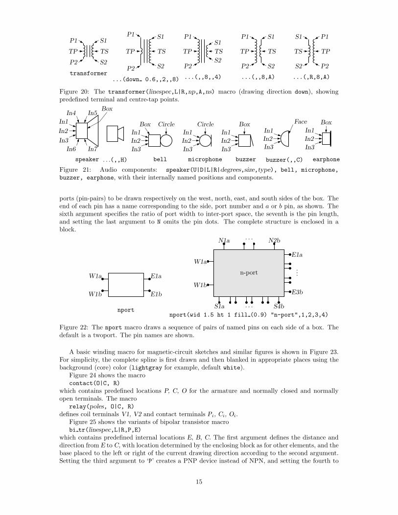
P1

P2

TP

S1

S2

TS

transformer

P1

P2

TP

S1

S2

TS

...(down 0.6,,2,,8)

P1

P2

TP

S1

S2

TS

...(,,8,,4)

P1

P2

TP

S1

S2

TS

...(,,8,A)

P1

P2

TP

S1

S2

TS

...(,R,8,A)

Figure 20: The transformer(linespec,L|R,np,A,ns) macro (drawing direction down), showingpredefined terminal and centre-tap points.

speaker

In1

In2

In3

In4 In5

In6 In7

Box

. . .(,,H) bell

In1

In2

In3

Box Circle

microphone

In1

In2

In3

Circle

buzzer

In1

In2

In3

Box

buzzer(,,C)

In1

In2

In3

Face

earphone

In1

In2

In3

Box

Figure 21: Audio components: speaker(U|D|L|R|degrees,size,type), bell, microphone,buzzer, earphone, with their internally named positions and components.

ports (pin-pairs) to be drawn respectively on the west, north, east, and south sides of the box. Theend of each pin has a name corresponding to the side, port number and a or b pin, as shown. Thesixth argument specifies the ratio of port width to inter-port space, the seventh is the pin length,and setting the last argument to N omits the pin dots. The complete structure is enclosed in ablock.

W1a

W1b

E1a

E1b

n-port

W1a

W1b

E1a

E3b

N1a N2b

S1a S4b

· · ·

· · ·

...

nportnport(wid 1.5 ht 1 fill (0.9) "n-port",1,2,3,4)

Figure 22: The nport macro draws a sequence of pairs of named pins on each side of a box. Thedefault is a twoport. The pin names are shown.

A basic winding macro for magnetic-circuit sketches and similar figures is shown in Figure 23.For simplicity, the complete spline is first drawn and then blanked in appropriate places using thebackground (core) color (lightgray for example, default white).

Figure 24 shows the macrocontact(O|C, R)

which contains predefined locations P, C, O for the armature and normally closed and normallyopen terminals. The macro

relay(poles, O|C, R)defines coil terminals V1, V2 and contact terminals Pi, Ci, Oi.

Figure 25 shows the variants of bipolar transistor macrobi tr(linespec,L|R,P,E)

which contains predefined internal locations E, B, C. The first argument defines the distance anddirection from E to C, with location determined by the enclosing block as for other elements, and thebase placed to the left or right of the current drawing direction according to the second argument.Setting the third argument to ‘P’ creates a PNP device instead of NPN, and setting the fourth to

15

winding

winding(R)

pitch

diam core wid

core color

T1 T2

gi1

−v1

+N1

i2

−v2

+N2

φ

Figure 23: The winding(L|R, diam, pitch, turns, core wid, core color) macro draws acoil with axis along the current drawing direction. Terminals T1 and T2 are defined. Setting thefirst argument to R draws a right-hand winding.

contact

P

O

C

contact(,R)

P

O

Ccontact(O,) contact(C,)

V1 V2

P1

O1

C1

relay

V1 V2

P1

O1

C1

P2

O2

C2

relay(2,,) relay(2,,R) relay(2,O,) relay(2,C,)

Figure 24: The contact(O|C,R) and relay(poles,O|C,R) macros (default direction right).

E

B

C

bi tr(up dimen )E

B

C

bi tr(,R)E

B

C

bi tr(,,P)E

B

C

bi tr(,,,E)E

G

C

igbtE

G

C

igbt(,,LD)

Figure 25: Bipolar transistor variants (current direction upward).

‘E’ draws an envelope around the device. Thus for example, the code fragment in Figure 26 placesa bipolar transistor, connects a ground to the emitter, and connects a resistor to the collector.

The bi tr and igbt macros are wrappers for the macro bi trans(linespec, L|R, chars, E),which draws the components of the transistor according to the characters in its third argument.For example, multiple emitters and collectors can be specified as shown in Figure 27.

Some FETs with predefined internal locations S, D, and G are also included, with similararguments to those of bi tr, as shown in Figure 28. In all cases the first argument is a linespec,and entering R as the second argument orients the G terminal to the right of the current drawingdirection. The macros in the top three rows of the figure are wrappers for the general macromosfet(linespec,R,characters,E). The third argument of this macro is a subset of the characters{BDEFGLQRSTZ}, each letter corresponding to a diagram component as shown in the bottom row ofthe figure. Preceding the characters B, G, and S by u or d adds an up or down arrowhead to thepin, and preceding T by d negates the pin. This system allows considerable freedom in choosing orcustomizing components, as illustrated in Figure 28.

A UJT macro with predefined internal locations B1, B2, and E is illustrated in Figure 29, and anSCR macro with predefined internal locations T1, T2, and G is illustrated in Figure 30. The number

16

S: dot; line left_ 0.1; up_

Q1: bi_tr(,R) with .B at Here

ground(at Q1.E)

line up 0.1 from Q1.C; resistor(right_ S.x-Here.x); dot

Figure 26: The bi tr(linespec,L|R,P,E) macro.

C

B

E

B

C

BU

uES S

bi trans(,,BCuEBUS)

C

B

E0E2 E1

Em2

bi trans(,,BCdE2BU)

E

B

C0 C2C1

Cm2

bi trans(,,BC2dEBU)

Figure 27: The bi trans(linespec,L|R,chars,E) macro. The sub-elements are specified by thethird argument. The substring En creates multiple emitters E0 to En. Collectors are similar.

j fet(right dimen ,,,E)

G

S D

j fet(,,P,)

G

S D

e fet(,R,,)

G

S D

e fet(,,P,)

d fet(,,,)

d fet(,,P,)

e fet(,,,S)

e fet(,,P,S)

d fet(,,,S)

d fet(,,P,S)

c fet(,,,) c fet(,,P)

mosfet(,,dGSDF,)

dG

FS D

. . .(,,LEDSQuB,)

L

EQ

uB

. . .(,,ZSDFdT,)Z

dT

. . .(,,LEDSuB)

G

S DBIRF4905

G

D

S

Figure 28: JFET, insulated-gate enhancement and depletion MOSFETS, and simplified versions,see [12]. These macros are wrappers that invoke the mosfet macro as shown in the bottom row.The two lower-right examples show custom devices, the first defined by omitting the substrateconnection, and the second defined using a wrapper and custom envelope.

of possible semiconductor symbols is very large, so these macros must be regarded as prototypes.Some other non-two-terminal macros are dot, which has an optional argument ‘at location’, theline-thickness macros, the fill macro, and crossover, which is a useful if archaic method to shownon-touching conductor crossovers, as in Figure 31.

B1

E

B2

ujt(up dimen ,,,E)

B1

E B2

ujt(,,P,)

B1

EB2

ujt(,R,,)

B1

EB2

ujt(,R,P,)

Figure 29: UJT devices, with current drawing direction up.

17

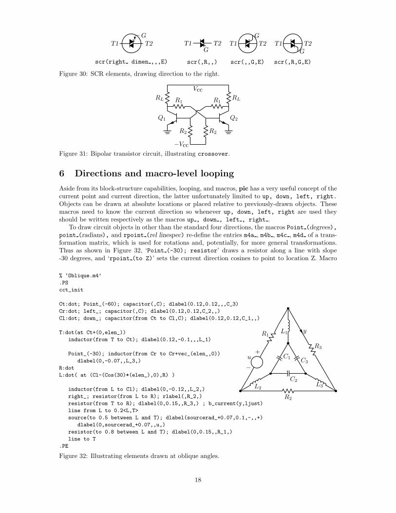
T1 T2G

scr(right dimen ,,,E)

T1 T2G

scr(,R,,)

T1 T2G

scr(,,G,E)

T1 T2G

scr(,R,G,E)

Figure 30: SCR elements, drawing direction to the right.

Q1 Q2

RL

VccRLR1 R1

R2

−Vcc

R2

Figure 31: Bipolar transistor circuit, illustrating crossover.

6 Directions and macro-level looping

Aside from its block-structure capabilities, looping, and macros, pic has a very useful concept of thecurrent point and current direction, the latter unfortunately limited to up, down, left, right.Objects can be drawn at absolute locations or placed relative to previously-drawn objects. Thesemacros need to know the current direction so whenever up, down, left, right are used theyshould be written respectively as the macros up , down , left , right .

To draw circuit objects in other than the standard four directions, the macros Point (degrees),point (radians), and rpoint (rel linespec) re-define the entries m4a , m4b , m4c , m4d of a trans-formation matrix, which is used for rotations and, potentially, for more general transformations.Thus as shown in Figure 32, ‘Point (-30); resistor’ draws a resistor along a line with slope-30 degrees, and ‘rpoint (to Z)’ sets the current direction cosines to point to location Z. Macro

% ‘Oblique.m4’

.PS

cct_init

Ct:dot; Point_(-60); capacitor(,C); dlabel(0.12,0.12,,,C_3)

Cr:dot; left_; capacitor(,C); dlabel(0.12,0.12,C_2,,)

Cl:dot; down_; capacitor(from Ct to Cl,C); dlabel(0.12,0.12,C_1,,)

T:dot(at Ct+(0,elen_))

inductor(from T to Ct); dlabel(0.12,-0.1,,,L_1)

Point_(-30); inductor(from Cr to Cr+vec_(elen_,0))

dlabel(0,-0.07,,L_3,)

R:dot

L:dot( at (Cl-(Cos(30)*(elen_),0),R) )

inductor(from L to Cl); dlabel(0,-0.12,,L_2,)

right_; resistor(from L to R); rlabel(,R_2,)

resistor(from T to R); dlabel(0,0.15,,R_3,) ; b_current(y,ljust)

line from L to 0.2<L,T>

source(to 0.5 between L and T); dlabel(sourcerad_+0.07,0.1,-,,+)

dlabel(0,sourcerad_+0.07,,u,)

resistor(to 0.8 between L and T); dlabel(0,0.15,,R_1,)

line to T

.PE

C3

C2

C1

L1

L3L2

R2

R3

y

−

+u

R1

Figure 32: Illustrating elements drawn at oblique angles.

18

vec (x,y) evaluates to the position (x,y) rotated by the argument of the previous Point , pointor rpoint command. The macro rvec (x,y) evaluates to position Here + vec (x,y) and is theprincipal device used to define relative locations in the circuit macros. Thus, line to rvec (x,0)draws a line of length x in the current direction.

macros. The source for the figure is shown, and illustrates that some hand-placement of labelsusing dlabel may be useful when elements are drawn obliquely. Because m4 macro argumentsare separated by commas, any commas that are integral parts of the arguments must be protected,either by parentheses as illustrated in inductor(from Cr to Cr+vec (elen ,0)), or by multiplesingle quotes, ‘‘,’’, as necessary. Commas also may be avoided by writing 0.5 between L andT instead of 0.5<L,T>.

Sequential location names such as In1, In2, . . . in logic and other diagrams can be generatedautomatically at the m4 processing stage. The libgen library defines the macro

for (start, end, increment, ‘actions’)for this purpose. Nested loops are allowed and the innermost loop index variable is m4x. Thefirst three arguments must be integers and the end value must be reached exactly; for example,for_(1,3,2,‘print In‘’m4x’) prints locations In1 and In3, but for_(1,4,2,‘print In‘’m4x’)does not terminate since the index takes on values 1, 3, 5, . . ..

7 Logic gates

Figure 33 shows the basic logic gates included in library liblog.m4. Gate macros have an optionalargument, an integer N from 0 to 16, defining locations In1, · · · InN, as illustrated for the NORgate in the figure. By default N = 2, except for macros NOT gate and BUFFER gate, which haveone input In1 unless they are given a first argument, which is treated as the line specification of atwo-terminal element.

Negated inputs or outputs are marked by circles drawn by the NOT_circle macro. The namemarks the point at the outer edge of the circle and the circle itself has the same name prefixed byN . For example, the output circle of a nand gate is named N Out and the outermost point of thecircle is named Out. The macro IOdefs creates a sequence of named outputs.

Gates are typically not two-terminal elements and are normally drawn horizontally or vertically(although arbitrary directions may be set with e.g. Point (degrees)). Each gate is contained in ablock of typical height 6*L unit where L unit is a macro intended to establish line separation foran imaginary grid on which the elements are superimposed.

Including an N in the second argument character sequence of any gate negates the inputs, andincluding B in the second argument invokes the general macro BOX gate([P|N]...,[P|N],horizsize,vert size,label), which draws box gates. Thus, BOX gate(PNP,N,,8,\geq 1) creates a gateof default width, eight L units height, negated output, three inputs with the second negated, andinternal label “≥ 1”. If the fifth argument begins with sprintf or a double quote then the argumentis copied literally; otherwise it is treated as scriptsize mathematics.

AND gate

OR gate

BUFFER gate

XOR gate

NAND gate

NOR gate(3)Out

N Out

In1In2In3

NOT gate

NXOR gate

&NAND gate(,B)

≥ 1NOR gate(3,NB)

= 1BOX gate(PN,N,,,=1)

=BOX gate(PP,N,,,=)

Figure 33: Basic logic gates. The input and output locations of a three-input NOR gate are shown.Inputs are negated by including an N in the second argument letter sequence. A B in the secondargument produces a box shape as shown in the rightmost column, where the second example hasAND functionality and the bottom two are examples of exclusive OR functions.

19

Y

Y

E

S0

S1

S2

I0 I1 I2 I3 I4 I5 I6 I7

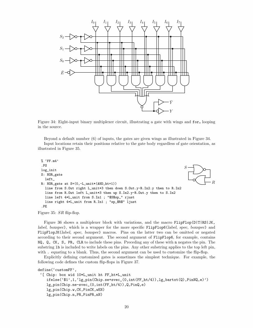
Figure 34: Eight-input binary multiplexer circuit, illustrating a gate with wings and for loopingin the source.

Beyond a default number (6) of inputs, the gates are given wings as illustrated in Figure 34.Input locations retain their positions relative to the gate body regardless of gate orientation, as

illustrated in Figure 35.

% ‘FF.m4’

.PS

log_init

S: NOR_gate

left_

R: NOR_gate at S+(0,-L_unit*(AND_ht+1))

line from S.Out right L_unit*3 then down S.Out.y-R.In2.y then to R.In2

line from R.Out left L_unit*3 then up S.In2.y-R.Out.y then to S.In2

line left 4*L_unit from S.In1 ; "$S$sp_" rjust

line right 4*L_unit from R.In1 ; "sp_$R$" ljust

.PE

S

R

Figure 35: SR flip-flop.

Figure 36 shows a multiplexer block with variations, and the macro FlipFlop(D|T|RS|JK,label, boxspec), which is a wrapper for the more specific FlipFlop6(label, spec, boxspec) andFlipFlopJK(label, spec, boxspec) macros. Pins on the latter two can be omitted or negatedaccording to their second argument. The second argument of FlipFlop6, for example, containsNQ, Q, CK, S, PR, CLR to include these pins. Preceding any of these with n negates the pin. Thesubstring lb is included to write labels on the pins. Any other substring applies to the top left pin,with . equating to a blank. Thus, the second argument can be used to customize the flip-flop.

Explicitly defining customized gates is sometimes the simplest technique. For example, thefollowing code defines the custom flip-flops in Figure 37.

define(‘customFF’,‘[ Chip: box wid 10*L_unit ht FF_ht*L_unit

ifelse(‘$1’,1,‘lg_pin(Chip.se+svec_(0,int(FF_ht/4)),lg_bartxt(Q),PinNQ,e)’)lg_pin(Chip.ne-svec_(0,int(FF_ht/4)),Q,PinQ,e)lg_pin(Chip.w,CK,PinCK,wEN)lg_pin(Chip.n,PR,PinPR,nN)

20

Q1

Q

Q

CK

D

FlipFlop(D,Q1)

Q2

Q

Q

CK

T

FlipFlop(T,Q2,ht h1 wid w1 fill (0.9))

Q

Q

S

R

FlipFlop(RS)

Q

Q

CK

PR

CLR

K

J

FlipFlop(JK)

Q

Q

CK

D

FlipFlop6(,DnCKQNQlb)

Q

CK

T

. . .(,TCKQlb)

Q

CK

CLR

K

J

FlipFlopJK(,JCKKQnCLRlb)

Mx1

Sel

0

1

2

3

Mux(4,Mx1)

In0

In1

In2

In3

Out

Sel

Sel0

1

2

3

Mux(4,,L)

Sel0

1

2

3

Mux(4,,T)

Sel

0

1

2

3

Mux(4,,LT)

Figure 36: The FlipFlop and Mux macros, with variations.

lg_pin(Chip.s,CLR,PinCLR,sN)lg_pin(Chip.sw+svec_(0,int(FF_ht/4)),R,PinR,w)lg_pin(Chip.nw-svec_(0,int(FF_ht/4)),S,PinS,w)

]’)

This definition makes use of macros L_unit and FF_ht that predifine dimensions and the logic-pinmacro lg_pin(location, printed label, pin name, type). The pin Q is drawn only if the macro

CK

PR

Q

Q

CLR

R

SSERIALINPUT

CLEAR

CLOCK

CK

PR

Q

Q

CLR

R

S

CK

PR

Q

Q

CLR

R

S

CK

PR

Q

Q

CLR

R

S

CK

PR

Q

CLR

R

S OUTPUT

PR4 PR3 PR2 PR1 PR0

PRESETENABLE

Figure 37: A 5-bit shift register.

21

argument is 1.A good strategy for drawing complex logic circuits might be summarized as follows:

• Establish the absolute locations of gates and other major components (e.g. chips) relative toa grid of mesh size commensurate with L unit, which is an absolute length.

• Draw minor components or blocks relative to the major ones, using parametrized relativedistances.

• Draw connecting lines relative to the components and previously-drawn lines.

• Write macros for repeated objects.

• Tune the diagram by making absolute locations relative, and by tuning the parameters. Someuseful macros for this are the following, which are in units of L unit:

AND ht, AND wd: the height and width of basic AND and OR gates

BUF ht, BUF wd: the height and width of basic buffers

N diam: the diameter of NOT circles

In addition to the logic gates described here, some experimental IC chip diagrams are included withthe distributed example files.

8 Element and diagram scaling

There are several issues related to scale changes. You may wish to use millimetres, for example,instead of the default inches. You may wish to change the size of a complete diagram while keepingthe relative proportions of objects within it. You may wish to change the sizes or proportionsof individual elements within a diagram. You must take into account that line widths are scaledseparately from drawn objects, and that the size of typeset text is independent of the pic language.

The scaling of circuit elements will be described first, then the pic scaling facilities.

8.1 Circuit scaling

The circuit elements all have default dimensions that are multiples of the pic environmental pa-rameter linewid, so changing this parameter changes default element dimensions. The scope of apic variable is the current block; therefore a sequence such as

resistor[ linewid = linewid*1.5; resistor ]resistor

produces a string of three resistors, the middle one larger than the other two. Alternatively, youmay redefine the default length elen or the body-size parameter dimen . For example, adding theline

define(‘dimen ’,dimen *1.2)after the cct init line of quick.m4 produces slightly larger element body sizes.

8.2 Pic scaling

There are at least three kinds of graphical elements to be considered:

1. The default sizes of linear and planar pic objects can be redefined by assigning values to thebuilt-in pic variables arcrad, arrowht, arrowwid, boxht, boxrad, boxwid, circlerad,dashwid, ellipseht, ellipsewid, lineht, linewid, moveht, movewid, textht, textwid.The · · ·ht and · · ·wid parameters refer to the default sizes of vertical and horizontal lines,moves, etc., except for arrowht and arrowwid, which refer to arrowhead dimensions. Theboxrad parameter can be used to put rounded corners on boxes.

22

Assigning a value to the variable scale multiplies all the built-in pic dimension variablesexcept arrowht, arrowwid, textht, and textwid by the new value of scale (gpic multipliesthem all). Thus the file quick.m4 can be modified to use millimetres as follows:

.PS # Pic input begins with .PSscale = 25.4 # mmcct_init # Set defaults

elen = 19 # Variables are allowed...

The .PS line can be used to scale the entire drawing, regardless of its interior. Thus, forexample, the line .PS 100/25.4 scales the entire drawing to a width of 100 mm. However,this method is not normally suitable for circuits because arrowheads, line widths, and textare treated differently.

If the final picture width exceeds the value of maxpswid, which has a default size of 8.5, thenthe picture is scaled to this value. Similarly if the height exceeds maxpsht, (default 11), thenthe picture is scaled to fit.

2. The finished size of typeset text is independent of pic variables, but can be determined as inSection 10. Thus, once dimensions x and y are known, then "text" wid x ht y assigns thedimensions of text.

3. Line widths are independent of diagram and text scaling, and have to be set independently.For example, the assignment linethick = 1.2 sets the default line width to 1.2 pt. Themacro linethick (points) is also provided, together with default macros thicklines andthinlines .

9 Writing macros

The m4 language is quite simple and is described in numerous documents such as the originalreference [7] or in later manuals [13]. If a new element is required, then modifying and renamingone of the library definitions or simply adding an option to it may suffice. Hints for drawing generaltwo-terminal elements are given in libcct.m4. However, if an element or composite is to be drawnin only one orientation then most of the elaborations used for general two-terminal elements inSection 4 can be dropped.

A macro is defined using quoted name and replacement text as follows:define(‘name’,‘replacement text’)After this line is read by the m4 processor, then whenever name is encountered as a separate

string, it is replaced by its replacement text, which may have multiple lines. The quotation charac-ters are used to defer macro expansion. Macro arguments are referenced inside a macro by number;thus $1 refers to the first argument.

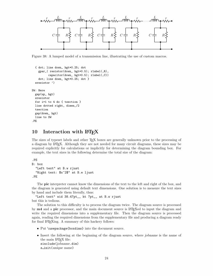
In the following example, two macros are defined to simplify the repeated drawing of a seriesresistor and series inductor, and the macro tsection defines a subcircuit that is replicated severaltimes to generate Figure 38.

% ‘Tline.m4’

.PS

cct_init

hgt = elen_*1.5

ewd = dimen_*0.9

define(‘sresistor’,‘resistor(right_ ewd); llabel(,r)’)

define(‘sinductor’,‘inductor(right_ ewd,W); llabel(,L)’)

define(‘tsection’,‘sinductor

23

r L

RC

r L

RC

r L

RC

r L

RC

r L

RC

r

Figure 38: A lumped model of a transmission line, illustrating the use of custom macros.

{ dot; line down_ hgt*0.25; dot

gpar_( resistor(down_ hgt*0.5); rlabel(,R),

capacitor(down_ hgt*0.5); rlabel(,C))

dot; line down_ hgt*0.25; dot }

sresistor ’)

SW: Here

gap(up_ hgt)

sresistor

for i=1 to 4 do { tsection }

line dotted right_ dimen_/2

tsection

gap(down_ hgt)

line to SW

.PE

10 Interaction with LATEX

The sizes of typeset labels and other TEX boxes are generally unknown prior to the processing ofa diagram by LATEX. Although they are not needed for many circuit diagrams, these sizes may berequired explicitly for calculations or implicitly for determining the diagram bounding box. Forexample, the text sizes in the following determine the total size of the diagram:

.PSB: box"Left text" at B.w rjust"Right text: $x^2$" at B.e ljust

.PE

The pic interpreter cannot know the dimensions of the text to the left and right of the box, andthe diagram is generated using default text dimensions. One solution is to measure the text sizesby hand and include them literally, thus:"Left text" wid 38.47pt__ ht 7pt__ at B.w rjust

but this is tedious.The solution to this difficulty is to process the diagram twice. The diagram source is processed

by m4 and a pic processor, and the main document source is LATEXed to input the diagram andwrite the required dimensions into a supplementary file. Then the diagram source is processedagain, reading the required dimensions from the supplementary file and producing a diagram readyfor final LATEXing. A summary of this hackery follows:

• Put \usepackage{boxdims} into the document source.

• Insert the following at the beginning of the diagram source, where jobname is the name ofthe main LATEX file:sinclude(jobname.dim)s init(unique name)

24

• Use the macro s box(‘text’) to produce typeset text of known size; alternatively, invoke themacros \boxdims and boxdim described below.

The macro s_box(‘text’) evaluates to"\boxdims{name}{text}" wid boxdim(name,w) ht boxdim(name,v)

On the second pass, this is equivalent to"text" wid x ht y

where x and y are the typeset dimensions of the LATEX input text. If s box is given two or morearguments then they are processed by sprintf.

The file boxdims.sty distributed with this package should be installed where LATEX can find it.The essential idea is to define a two-argument macro \boxdims that writes out definitions for thewidth, height and depth of its typeset second argument into file jobname.dim, where jobname is thename of the main source file. The first argument of \boxdims is used to construct unique symbolicnames for these dimensions. Thus, the line

box "\boxdims{Q}{\Huge Hi there!}"has the same effect as

box "\Huge Hi there!"except that the line

define(‘Q w’,77.6077pt )define(‘Q h’,17.27779pt )define(‘Q d’,0.0pt )dnlis written into file jobname.dim (and the numerical values depend on the current font).

Recent versions of boxdims.sty include the macro\boxdimfile{dimension file}

for specifying an alternative to jobname.dim as the dimension file to be written. This simplifiescases where jobname is not known in advance or where an absolute path name is required.

Another simplification is available. Instead of the sinclude(dimension file) line above, thedimension file can be read by m4 before reprocessing the source for the second time:

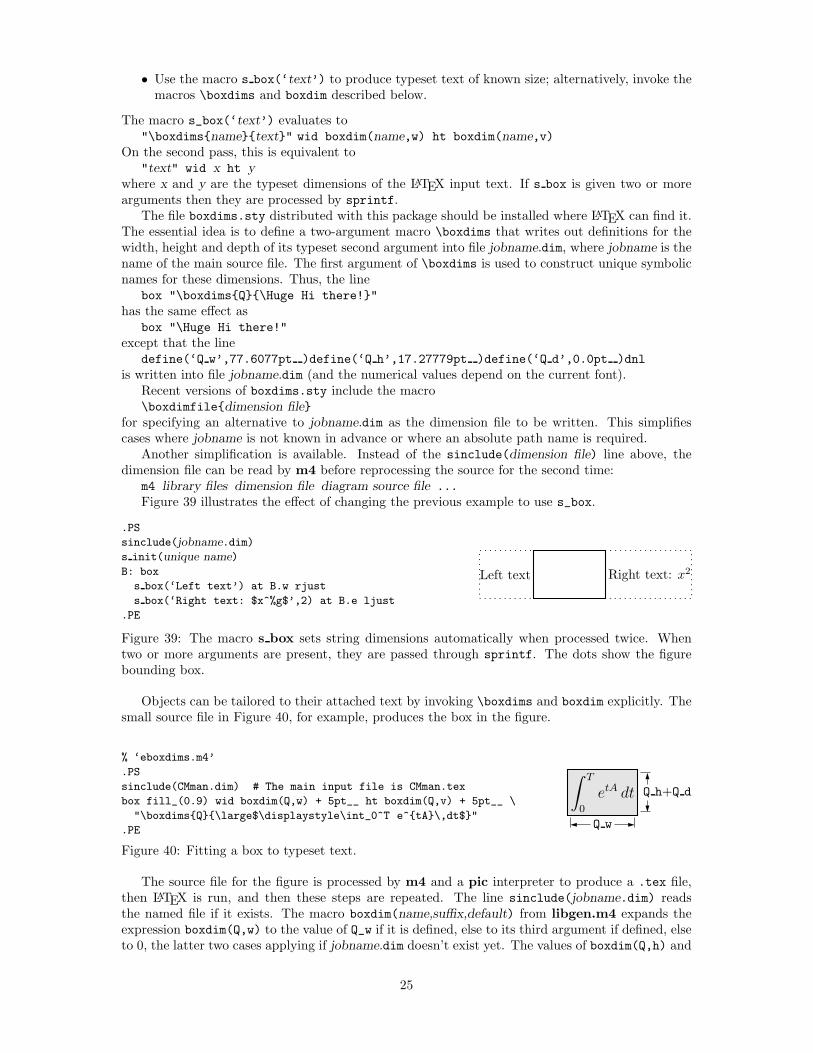
m4 library files dimension file diagram source file ...Figure 39 illustrates the effect of changing the previous example to use s_box.

.PS

sinclude(jobname.dim)s init(unique name)B: box

s box(‘Left text’) at B.w rjust

s box(‘Right text: $x^%g$’,2) at B.e ljust

.PE

Left text Right text: x2

Figure 39: The macro s box sets string dimensions automatically when processed twice. Whentwo or more arguments are present, they are passed through sprintf. The dots show the figurebounding box.

Objects can be tailored to their attached text by invoking \boxdims and boxdim explicitly. Thesmall source file in Figure 40, for example, produces the box in the figure.

% ‘eboxdims.m4’

.PS

sinclude(CMman.dim) # The main input file is CMman.tex

box fill_(0.9) wid boxdim(Q,w) + 5pt__ ht boxdim(Q,v) + 5pt__ \

"\boxdims{Q}{\large$\displaystyle\int_0^T e^{tA}\,dt$}"

.PE

∫ T

0

etA dt

Q w

Q h+Q d

Figure 40: Fitting a box to typeset text.

The source file for the figure is processed by m4 and a pic interpreter to produce a .tex file,then LATEX is run, and then these steps are repeated. The line sinclude(jobname.dim) readsthe named file if it exists. The macro boxdim(name,suffix,default) from libgen.m4 expands theexpression boxdim(Q,w) to the value of Q_w if it is defined, else to its third argument if defined, elseto 0, the latter two cases applying if jobname.dim doesn’t exist yet. The values of boxdim(Q,h) and

25

boxdim(Q,d) are similarly defined, and for convenience, boxdim(Q,v) evaluates to the sum of these.Macro pt__ is defined as *scale/72.27 in libgen.m4, to convert points to drawing coordinates.

The argument of s init, which should be unique within jobname.dim, is used to generate aunique \boxdims first argument for each invocation of s_box in the current file. If s_init has beenomitted, the symbols “!!” are inserted into the text as a warning. Be sure to quote any commasin the arguments. Since the first argument is LATEX source, make a rule of quoting it to avoidcomma and name-clash problems. For convenience, the macros s ht, s wd, and s dp evaluate tothe dimensions of the most recent s box string or to the dimensions of their argument names, ifpresent.

More tricks can be played. The exampleS: s_box(‘\includegraphics{file.eps}’) with .sw at location

shows a nice way of including eps graphics in a diagram. The included picture (named S in theexample) has known position and dimensions, which can be used to add vector graphics or text tothe picture. To aid in overlaying objects, the macro boxcoord(object name, x-fraction, y-fraction)evaluates to a position, with boxcoord(object name,0,0) at the lower left corner of the object,and boxcoord(object name,1,1) at its upper right.

11 PSTricks tricks

This section applies only to a pic processor (dpic) that is capable of producing PSTricks output.Arbitrary PSTricks commands can be mixed with m4 input to create complicated effects, butsome commonly required effects are particularly simple.

The rotation of text is illustrated by the file

% ‘Axes.m4’

.PS

arrow right 0.7 "‘$x$-axis’" below

arrow up 0.7 from 1st arrow.start "‘\rput[B]{90}(0,0){$y$-axis}’" rjust

.PE

which produces horizontal text, and text rotated 90◦ along the vertical line.Another common requirement is the filling of arbitrary shapes, as illustrated by the following

lines within a .m4 file:

command "‘\pscustom[fillstyle=solid,fillcolor=lightgray]{’"drawing commands for an arbitrary closed curvecommand "‘}%’"

The macro shade(gray value,closed line specs) can be invoked to accomplish the same effect asthe above example.

For colour printing or viewing, arbitrary colours can be chosen, as described in the PSTricksmanual. PSTricks parameters can be set by inserting the line

command "‘\psset{option=value, · · ·}’"in the drawing commands or by using the macro psset (PSTricks options).

12 Web documents, pdf, and alternative output formats

Circuit diagrams contain graphics and symbols, and the issues related to web publishing are similarto those for other mathematical documents. Here the important factor is that gpic -t gener-ates output containing tpic \special commands, which must be converted to the desired output,whereas dpic can generate several alternative formats. One of the easiest methods for producingweb documents is to generate postscript as usual and to convert the result to pdf format with AdobeDistiller or equivalent.

PDFlatex produces pdf without first creating a postscript file but does not handle tpic \specials,so dpic must be installed.

26

Most PDFLatex distributions are not directly compatible with PSTricks, but the Tikz PGFoutput of dpic is compatible with both LATEX and PDFLatex. Several alternative dpic outputformats such as mfpic and MetaPost also work well. To test MetaPost, create a file filename.mpcontaining appropriate header lines, for example:

verbatimtex\documentclass[11pt]{article}\usepackage{times,boxdims,graphicx}\boxdimfile{tmp.dim}\begin{document} etex

Then append one or more diagrams by using the equivalent ofm4 <path>mpost.m4 library files diagram.m4 | dpic -s >> filename.mpThe command “mpost --tex=latex filename.mp end” processes this file, formatting the di-

agram text by creating a temporary .tex file, LATEXing it, and recovering the .dvi output tocreate filename.1 and other files. If the boxdims macros are being invoked, this process must berepeated to handle formatted text correctly as described in Section 10. In this case, either putsinclude(tmp.dim) in the diagram .m4 source or read the .dim file at the second invocation ofm4 as follows:

m4 <path>mpost.m4 library files tmp.dim diagram.m4 | dpic -s >> filename.mpOn some operating systems the absolute path name for tmp.dim has to be used to ensure that

the correct dimension file is written and read. This distribution includes a Makefile that simplifiesthe process; otherwise a script can automate it.

Having produced filename.1, rename it to filename.mps and, voila, you can now run PDFlatexon a .tex source that includes the diagram using \includegraphics{filename.mps} in the usualway.

The Dpic processor is capable of other output formats, as illustrated in Figure 41 and in examplefiles included with the distribution. The LATEX drawing commands alone or with eepic or pict2eextensions are suitable only for simple diagrams.

LATEXLATEXpict2e

LATEXPSTricks

LATEXor

PDFlatextikz

LATEXMfpic

Metafont

MetaPost

LATEXor

PDFlatex

LATEXpsfrag

tpic\special

.tex

LATEX.tex

-e

PSTricks.tex

-p

PGF.tex

-g

mfpic.tex

-m

MetaPost.mp

-s

Postscriptpsfrag

.eps

-f

Postscript.eps

-r

Xfig.fig

-x

dpicgpic -t m4

Diagram source Macro libraries

Figure 41: Output formats produced by gpic -t and dpic.

13 Developer’s notes

Several years ago in the course of writing a book, I took a few days off to write a pic-like interpreter(dpic) to automate the tedious coordinate calculations required by LATEX picture objects. Themacros in this distribution and the interpreter are the result of that effort and of drawings I have hadto produce since. The interpreter has been upgraded over time to generate mfpic, MetaPost [5],raw Postscript, Postscript with PSfrag tags, and PSTricks output, the latter my preference

27

because of its quality and flexibility, including facilities for colour and rotations, together withsimple font selection. In addition, xfig-compatible output has been added and, most recently, TikZPGF output, which combines the simplicity of PSTricks with PDFlatex compatibility. Instead ofpic macros I preferred the equally simple but more powerful m4 macro processor, and thereforem4 is required here, although dpic now supports pic-like macros. Free versions of m4 are availablefor Unix, Windows, and other operating systems.

If starting over today would I not just use one of the other drawing packages available thesedays? It would depend on the context, but pic remains a good choice for the geometrical calculationsthat are necessary for precision in line drawings. The language is also simple to learn and, moreimportantly, to read. There are built-in looping and block-structure constructs that combine powerwith simplicity, and the language has stood the test of time. However, no choice of tool is withoutcompromise, and making good graphics is time-consuming no matter how it is done.

The dpic interpreter has several output-format options that may be useful. The eepicemu andpict2e extensions of the primitive LATEX picture objects are supported. The mfpic output allowsthe production of Metafont alphabets of circuit elements or other graphics, thereby essentiallyremoving dependence on device drivers, but with the complication of treating every alphabeticcomponent as a TEX box. The xfig output allows elements to be precisely defined with dpic andinteractively placed with xfig. Dpic will also issue low-level MetaPost or Postscript commands,so that diagrams defined using pic can be manipulated and combined with others. The Postscriptoutput is compatible with CorelDraw r©, and by extension to Adobe Illustrator r©. The user isresponsible for ensuring that the correct fonts are provided and for reformatting labels.

14 Bugs

The distributed macros are not written for maximum robustness. Macro arguments could be testedfor correctness and explanatory error messages could be written as necessary, but that would makethe macros more difficult to read and to write. You will have to read them when unexpected resultsare obtained or when you wish to modify them.

In response to suggestions, some of the macros have been modified to allow easier customizationto forms not originally anticipated, but this process is not complete.

Here are some hints, gleaned from experience and from comments I have received.

1. Initialization: If the first element macro evaluated is non-two-terminal or is within a Picblock, then later macros evaluated outside the block may produce the error message

there is no variable ‘rp ang’

because rp ang is not defined in the outermost scope of the diagram. To cure this problem,put the line

cct init

immediately after the .PS line or prior to the first block. It is entirely permissible to modifycct init to include commonly-used diagram initializations, such as the thicklines state-ment, and to invoke cct init at the beginning of every diagram. For completeness, macrosgen init, log init, darrow init are also provided for cases where the circuit library is notneeded.

2. Pic objects versus macros: A common error is to write something like

line from A to B; resistor from B to C

when it should be

line from A to B; resistor(from B to C)

This error is caused by an unfortunate inconsistency between the linear pic objects and theway m4 passes macro arguments.

3. Commas: Remember that macro arguments are separated by commas, and commas that arepart of an argument must be protected by parentheses or quotes. Thus,

28

shadebox(box with .n at w,h)

produces an error, whereas

shadebox(box with .n at w‘,’h)

and

shadebox(box with .n at (w,h))

do not.

4. Default lengths: Remember that the linespec argument of element macros requires both adirection and a length. Writing

source(up )

draws a source up a distance equal to the current lineht value, which may cause confusion.It is usually better to specify both the direction and length of an element, thus:

source(up elen ).

5. Quotes: Single quote characters are stripped in pairs by m4, so the string

"‘‘inverse’’"

will be typeset as if it were

"‘inverse’".

The cure is to add single quotes.

The most subtle part of writing m4 macros is deciding when to quote arguments. In thecontext of circuits it seemed best to assume that macro arguments would not be protected byquotes at the level of macro invocation, but should be quoted inside each macro. There maybe cases where this rule is not optimal.

6. Dollar signs: The i-th argument of an m4 macro is $i, where i is an integer, so the followingconstruction can cause an error when it is part of a macro,

"$0$" rjust below

since $0 expands to the name of the macro itself. To avoid this problem, put the string inquotes or write "$‘’0$".

7. Name conflicts: Using the name of a macro as part of a comment or string is a simple andcommon error. Thus,

arrow right "$\dot x$" above

produces an error message because dot is a macro name. Macro expansion can be avoided byadding quotes, as follows:

arrow right ‘"$\dot x$"’ above

Library macros intended only for internal use have names that begin with m4 to avoid nameclashes, but in addition, a good rule is to quote all LATEX in the diagram input.

If extensive use of strings that conflict with macro names is required, then one possibility isto replace the strings by macros to be expanded by LATEX, for example the diagram

.PS

box "\stringA"

.PE

with the LaTeX macro

\newcommand{\stringA}{

Circuit containing planar inductor and capacitor}

29

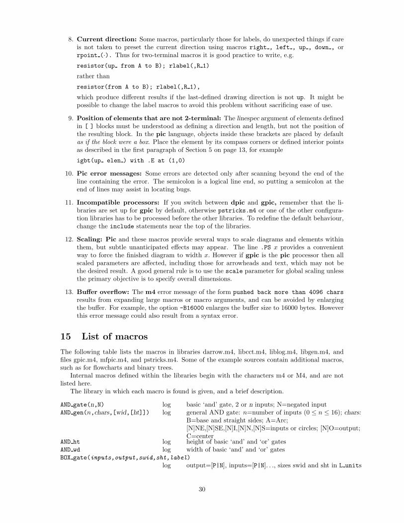
8. Current direction: Some macros, particularly those for labels, do unexpected things if careis not taken to preset the current direction using macros right , left , up , down , orrpoint (·). Thus for two-terminal macros it is good practice to write, e.g.

resistor(up from A to B); rlabel(,R 1)

rather than

resistor(from A to B); rlabel(,R 1),

which produce different results if the last-defined drawing direction is not up. It might bepossible to change the label macros to avoid this problem without sacrificing ease of use.

9. Position of elements that are not 2-terminal: The linespec argument of elements definedin [ ] blocks must be understood as defining a direction and length, but not the position ofthe resulting block. In the pic language, objects inside these brackets are placed by defaultas if the block were a box. Place the element by its compass corners or defined interior pointsas described in the first paragraph of Section 5 on page 13, for example

igbt(up elen ) with .E at (1,0)

10. Pic error messages: Some errors are detected only after scanning beyond the end of theline containing the error. The semicolon is a logical line end, so putting a semicolon at theend of lines may assist in locating bugs.

11. Incompatible processors: If you switch between dpic and gpic, remember that the li-braries are set up for gpic by default, otherwise pstricks.m4 or one of the other configura-tion libraries has to be processed before the other libraries. To redefine the default behaviour,change the include statements near the top of the libraries.

12. Scaling: Pic and these macros provide several ways to scale diagrams and elements withinthem, but subtle unanticipated effects may appear. The line .PS x provides a convenientway to force the finished diagram to width x. However if gpic is the pic processor then allscaled parameters are affected, including those for arrowheads and text, which may not bethe desired result. A good general rule is to use the scale parameter for global scaling unlessthe primary objective is to specify overall dimensions.

13. Buffer overflow: The m4 error message of the form pushed back more than 4096 charsresults from expanding large macros or macro arguments, and can be avoided by enlargingthe buffer. For example, the option -B16000 enlarges the buffer size to 16000 bytes. Howeverthis error message could also result from a syntax error.

15 List of macros

The following table lists the macros in libraries darrow.m4, libcct.m4, liblog.m4, libgen.m4, andfiles gpic.m4, mfpic.m4, and pstricks.m4. Some of the example sources contain additional macros,such as for flowcharts and binary trees.

Internal macros defined within the libraries begin with the characters m4 or M4, and are notlisted here.

The library in which each macro is found is given, and a brief description.

AND gate(n,N) log basic ‘and’ gate, 2 or n inputs; N=negated inputAND gen(n,chars,[wid,[ht]]) log general AND gate: n=number of inputs (0 ≤ n ≤ 16); chars:

B=base and straight sides; A=Arc;[N]NE,[N]SE,[N]I,[N]N,[N]S=inputs or circles; [N]O=output;C=center

AND ht log height of basic ‘and’ and ‘or’ gatesAND wd log width of basic ‘and’ and ‘or’ gatesBOX gate(inputs,output,swid,sht,label)

log output=[P|N], inputs=[P|N]. . ., sizes swid and sht in L units

30

BUFFER gate(linespec, N) log basic buffer, 1 input or as a 2-terminal element, N=negated inputBUFFER gen(chars,wd,ht,[N|P]*,[N|P]*,[N|P]*)

log general buffer, chars: T=triangle, [N]O=output location Out (NOdraws circle N Out); [N]I, [N]N, [N]S, [N]NE, [N]SE inputlocations; C=centre location. Args 4-6 allow alternativedefinitions of respective In, NE, and SE argument sequences

BUF ht log basic buffer gate heightBUF wd log basic buffer gate widthCos(integer) gen cosine function, integer degreesE gen the constant eFector(x1,y1,z1,x2,y2,z2) 3D vector projected on current view plane with top face of

3-dimensonal arrowhead normal to x2,y2,z2FlipFlop(D|T|RS|JK, label, boxspec)

log flip-flops, boxspec=e.g. ht x wid yFlipFlop6(label, spec, boxspec) log 6-input flip-flops, spec=[[n]NQ][[n]Q][[n]CK][[n]PR][lb]

[[n]CLR][[n]S][[n].|D|T|R] to include and negate pins, lb toprint labels

FlipFlopJK(label, spec,boxspec) log JK flip-flop, spec similar to aboveG hht log gate half-heightHOMELIB all directory containing librariesIOdefs(linespec,label,[P|N]*,L|R)

log Define locations label1, . . . labeln along the line; P= label only;N=with NOT circle; R=circle to right of current direction

Intersect (Name1,Name2) gen intersection of two named linesL unit log logic-element grid sizeLH symbol(U|D|L|R|degrees) log logic-gate hysteresis symbolLT symbol(U|D|L|R|degrees) log logic-gate triangle symbolMax(arg, arg, . . .) gen Max of an arbitrary number of inputsMin(arg, arg, . . .) gen Min of an arbitrary number of inputsMux(n, label, [L][T]) gen binary multiplexer, n inputs, L reverses pin numbers, T puts Sel

pin to topNAND gate(n,N) log ‘nand’ gate, 2 or n inputs; N=negated inputNOR gate(n,N) log ‘nor’ gate, 2 or n inputs; N=negated inputNOT gate(linespec,N) log ‘not’ gate, 1 input or as a 2-terminal element, N=negated inputNXOR gate(n,N) log ‘nxor’ gate, 2 or n inputs; N=negated inputNOT circle log ‘not’ circleN diam log diameter of ‘not’ circlesOR gate(n,N) log ‘or’ gate, 2 or n inputs; N=negated inputOR gen(n,chars,[wid,[ht]]) log general OR gate: n=number of inputs (0 ≤ n ≤ 16); chars:

B=base and straight sides; A=Arcs;[N]NE,[N]SE,[N]I,[N]N,[N]S=inputs or circles; [N]P=XOR arc;[N]O=output; C=center

Point (integer) gen sets direction cosines in degreesRect (radius,angle) gen (deg) polar-to-rectangular conversionSin(integer) gen sine function, integer degreesXOR gate(n,N) log ‘xor’ gate, 2 or n inputs; N=negated inputabove gen string position above relative to current directionabs (number) gen absolute value functionamp(linespec,size) cct amplifierantenna(at location, T, A|L|T|S|D|P|F, U|D|L|R|degrees)

cct antenna, without stem for nonblank 2nd arg; A=aerial, L=loop,T=triangle, S=diamond, D=dipole, P=phased, F=fork; up, down,left, right, or angle from horizontal (default -90)

arca(chord linespec, ccw|cw, radius, modifiers)gen arc with acute angle (obtuse if radius is negative)

arcr(center,radius,start angle,end angle)

31

gen arc definition, e.g., arc(A,r,0,pi /2) cw ->arcd(center,radius,start degrees,end degrees)

gen arc definition (see arcr), angles in degreesarrowline(linespec) cct line (dotted, dashed permissible) with centred arrowheadbattery(linespec,n,R) cct n-cell battery: default 1 cell, R=reversed polaritybeginshade(gray value) gen begin gray shading, see shade e.g., beginshade(.5); closed line

specs; endshadebell( U|D|L|R|degrees, size) cct bell, In1 to In3 definedbelow gen string position relative to current directionbi tr(linespec,L|R,P,E) cct left or right, N or P-type bipolar transistor, without or with

envelopebi trans(linespec,L|R,chars,E) cct bipolar transistor core left or right; chars: BU=bulk line; B=base

line and label; S=Schottky base hooks; uEn|dEn=emitters E0 toEn; uE|dE=single emitter; Cn=collectors C0 to Cn; C=singlecollector; G=gate line and location; H=gate line; L=L-gate lineand location; [d]D=named parallel diode, d=dotted connection

boxcoord(planar obj,x fraction,y fraction)gen internal point in a planar object

boxdim(name,h|w|d|v,default) gen evaluate, e.g. name w if defined, else default if given, else 0 v givessum of d and h values

bp gen big-point-size factor, in scaled inches, (*scale/72)buzzer( U|D|L|R|degrees, size,[C])

cct buzzer, In1 to In3 defined, C=curvedb current(label,pos,In|Out,Start|End,frac)

cct labelled branch-current arrow to frac between branch end and bodyc fet(linespec,L|R,P) cct left or right, plain or negated pin simplified MOSFETcapacitor(linespec,C,R) cct capacitor, C=curved-plate, E=polarized boxed plates,

K=filled boxed plates, R=reversed polaritycbreaker(linespec, L|R, D) cct circuit breaker to left or right, D=dottedclabel(label,label,label) cct centre triple labelcontact(O|C,R) cct single-pole contact: default double pole or normally open or

closed, oriented to the left or rightcontline(line) gen evaluates to continue if processor is dpic, otherwise to first arg

(default line)consource(linespec,V|I) cct voltage or current controlled sourcecosd(arg) gen cosine of an expression in degreescross(at location) gen plots a small crosscross3D(x1,y1,z1,x2,y2,z2) 3D cross product of two triplescrossover(linespec, L|R, Line1, ...)

cct line jumping left or right over named linescrosswd gen cross dimensioncsdim cct controlled-source widthd fet(linespec,L|R,P,S,E|S) cct left or right, N or P depletion MOSFET, normal or simplified,

without or with envelope or thick channeldabove(at location) darrow above (displaced dlinewid/2)darrow(linespec,t,t,width,arrowhd wd,arrowhd ht, <- or <-| or |)

darrow double arrow, truncated at beginning or end, specified sizes,reversed arrowhead or closed stem

dashline(linespec,thickness|color|<->,dash len, gap len,G)gen dashed line with dash at end (G ends with gap)

dbelow(at location) darrow below (displaced dlinewid/2)dcosine3D(i,x,y,z) 3D extract i-th entry of triple x,y,zdelay(linespec,size) cct delay elementdelay rad cct delay radiusdend(at location) darrow close (or start) double linediff (a,b) gen difference function

32

diff3D(x1,y1,z1,x2,y2,z2) 3D difference of two triplesdimen cct size parameter for circuit elementsdimension (linespec,offset,label,D|H|W|blank width,tic offset,arrowhead )

gen macro for dimensioning diagrams; arrowhead=-> | <-diode(linespec,B|D|L|LE[R]|P[R]|S|T|Z,[R][E])

cct diode: bi-directional, diac, Schottky, tunnel, zener, LED (right),photodiode (right), open; R=reversed polarity, E=enclosure

direction (U|D|L|R|degrees, default)gen sets current direction up, down, left, right, or angle in degrees.

dlabel(long,lat,label,label,label)cct general triple label

dleft darrow double line left turndline(linespec,t,t,width, |-| or -| or |-)

darrow double line, truncated by half width at either end, closed at eitheror both ends

dlinewid darrow width of double linesdljust(at location) darrow ljust (displaced dlinewid/2)dn gen sets down relative to current-directiondot(at location,radius,fill) gen filled circle (third arg= gray value: 0=black, 1=white)dot3D(x1,y1,z1,x2,y2,z2) 3D dot product of two triplesdotrad gen dot radiusdown gen sets current direction to downdright darrow double arrow right turndrjust(at location) darrow rjust (displaced dlinewid/2)dswitch(linespec,L|R,W[ud]B[K]chars)

cct SPST switch left or right, W=baseline, B=contact blade,dB=contact blade to the right of drawing direction, K=verticalclosing contact line, C = external operating mechanism, D =dotted contact, E = emergency button, EL = early close (or lateopen), LE = late close (or early open), F = fused, H = time delayclosing, uH = time delay opening, HH = time delay opening andclosing, K = vertical closing contact, L = limit, M = maintained(latched), MM = momentary contact on make, MR = momentarycontact on release, MMR = momentary contact on make andrelease, O = hand operation button, P = pushbutton, T =thermal control linkage, Y = pull switch, Z = turn switch

dtee([L|R]) darrow double arrow tee junction with tail to left, right, or (default) backalong current direction

dtor gen degrees to radians conversion constantdturn(degrees ccw) darrow turn dline arg1 degrees left (ccw)e gen .e relative to current directione fet(linespec,L|R,P,S,E|S) cct left or right, N or P enhancement MOSFET, normal or simplified,

without or with envelope or thick channelearphone( U|D|L|R|degrees, size)

cct earphone, In1 to In3 definedebox(linespec,length,ht,fill value)cct two-terminal box element with adjustable dimensions and fill

value 0 (black) to 1 (white)eleminit (linespec) cct internal line initializationelen cct default element lengthem arrows([N|I|E][D],angle,length)

cct radiation arrows N=nonionizing, I=ionizing, E=simple; D=dotendshade gen end gray shading, see beginshadeexpe gen exponential, base efill (number) gen fill macro, 0=black, 1=whitefor (start,end,increment,‘actions’)

gen integer for loop with index variable m4x

33

fuse(linespec, type, wid, ht) cct fuse symbol, type= A|B|C|D|S|HB|HC or dA=Dgap(linespec,fill,A) cct gap with (filled) dots, A=chopped arrow between dotsglabel cct internal general labellergpar (element,element,separation)

cct two same-direction elements in parallelgpic gpic defined to signify gpic is being usedgrid (x,y) log absolute grid locationground(at location, T, N|F|S|L|P|E, U|D|L|R|degrees)

cct ground, without stem for nonblank 2nd arg; N=normal, F=frame,S=signal, L=low-noise, P=protective, E=European; up, down,left, right, or angle from horizontal (default -90)

hop(L|R,at location) cct conductor crossing another to left or righthoprad cct hop radiusht gen height relative to current directionigbt(linespec,L|R,[L][[d]D]) cct left or right IGBT, L=alternate gate type, D=parallel diode,

dD=dotted connectionsinductor(linespec,W,n,M) cct inductor, narrow or wide, 4 or n arcs, without or with magnetic

coreintegrator(linespec,size) cct integrating amplifierintersect (line1.start,line1.end,line2.start,line2.end)

gen intersection of two linesj fet(linespec,L|R,P,E) cct left or right, N or P JFET, without or with envelopelarrow(label,->|<-,dist) cct arrow dist to left of last-drawn 2-terminal elementlbox(wid, ht, type) gen box oriented in current direction, type= e.g. dottedleft gen left with respect to current directionlength3D(x,y,z) 3D Euclidean length of triple x,y,zlg pin(location, logical name, pin label, n|e|s|w[N|L|M][E], pinno, optlen)

log comprehensive logic pin; n|e|s|w=direction, N=negated,L=active low out, M=active low in, E=edge trigger

linethick (number) gen set line thickness in pointslin leng(line-reference) gen calculate the length of a lineljust gen ljust with respect to current directionllabel(label,label,label) cct triple lable on left side of the elementloc (x, y) gen location adjusted for current directionlog10E gen constant log10(e)loge gen logarithm, base elt gen left with respect to current directionmanhattan gen sets direction cosines for left, right, up, downmfpic mfpic defined to signify mfpic is being usedmicrophone( U|D|L|R|degrees, size)

cct microphone, In1 to In3 definedmosfet(linespec,L|R,chars,E) cct MOSFET left or right, included components defined by

characters, envelopem4lstring(arg1,arg2) gen expand arg1 if it begins with sprintf or ", otherwise arg2m4 arrow(linespec,ht,wid) gen arrow with adjustable head, filled when possiblem4xtract(‘string1’,string2) gen delete string2 from string1, return 1 if presentn gen .n with respect to current directionne gen .ne with respect to current directionneg gen unary negationnport(box spec,nw,nn,ne,ns,space ratio,pin lgth,style)

cct nport macro (default 2-port)nw gen .nw with respect to current directionopamp(linespec,label,label,size,[P][R])

cct operational amplifier with −, + or other internal labels, specifiedsize. P adds power connections, R swaps In1, In2 labels

open arrow(linespec,ht,wid) gen arrow with adjustable open head

34

par (element,element,separation) cct two same-direction, same-length elements in parallelpoint (angle) gen (radians) set direction cosinespolar (x,y) gen rectangular-to polar conversionpotentiometer(linespec,cycles,fractional pos,length,· · ·)

cct resistor with taps T1, T2, . . . with specified fractional positionsand lengths (possibly neg)

print3D(x,y,z) 3D write out triple for debuggingprod (a,b) gen binary multiplicationproject(x,(y,(z) 3D 3D to 2D projectionpsset (PSTricks settings) gen set PSTricks parameterspstricks pstricks defined to signify PSTricks is being usedpt gen TEX point-size factor, in scaled inches, (*scale/72.27)rarrow(label,->|<-,dist) cct arrow dist to right of last-drawn 2-terminal elementrect (radius,angle) gen (radians) polar-rectangular conversionrelay(n,O|C,R) cct relay: n poles (default 1), default double throw or normally open

or closed, drawn left or right of current directionresistor(linespec,n|E,chars) cct resistor, n cycles (default 3), chars: E=ebox, Q=offset, H=squared,

R=right-orientedreversed(‘macro name’,args) cct reverse polarity of 2-terminal elementright gen set current direction rightrjust gen right justify with respect to current directionrlabel(label,label,label) cct triple lable on right side of the elementrot3Dx(radians,x,y,z) 3D rotates x,y,z about x axisrot3Dy(radians,x,y,z) 3D rotates x,y,z about y axisrot3Dz(radians,x,y,z) 3D rotates x,y,z about z axisrpoint (linespec) gen set direction cosinesrpos (position) gen Here + positionrt gen right with respect to current directionrtod gen constant, degrees/radianrvec (x,y) gen location relative to current directions gen .s with respect to current directions box(text,expr1,· · ·) gen generate dimensioned text string using \boxdims from

boxdims.sty. Two or more args are passed to sprintf()s dp(name,default) gen depth of the most recent (or named) s boxs ht(name,default) gen height of the most recent (or named) s boxs init(name) gen initialize s box string label to name which should be uniques wd(name,default) gen width of the most recent (or named) s boxscr(linespec,R,G,E) cct triac (scr), right, gated, envelopese gen .se with respect to current directionsetview(azimuth degrees,elevation degrees)

3D set projection viewpointsfg init(default line len, node rad, arrowhd len, arrowhd wid)

cct initialization of signal flow graph macrossfgabove cct like above but with extra spacesfgbelow cct like below but with extra spacesfgarc(linespec,text,text justification,cw|ccw,height scale factor)

cct directed arc drawn between nodes, with text label and aheight-adjustment parameter

sfgline(linespec,text,text justification)cct directed straight line chopped by node radius, with text label

sfgnode(at location,text,above|below)cct white small circle, with text label

sfgself(at location, U|D|L|R|degrees, text, text justification, cw|ccw, scale factor)cct self-loop drawn at angle angle from a node, with text label and a

size-adjustment parametershade(gray value,closed line specs)

35

gen fill arbitrary closed curveshadebox(box specification) gen box with edge shadingsign (number) gen sign functionsind(arg) gen sine of an expression in degreessource(linespec,V|v|I|i|AC|G|Q|X|string,diameter)

cct source, blank or voltage (2 types) or current (2 types) or AC or Gor Q or X or labelled

sourcerad cct default source radiussprod3D(a,x,y,z) 3D scalar product of triple x,y,z by asp gen evaluates to medium space for gpic stringsspeaker( U|D|L|R|degrees,size,H)

cct speaker, In1 to In7 defined; H=hornsum (a,b) gen binary sumsum3D(x1,y1,z1,x2,y2,z2) 3D sum of two triplessvec (x,y) log scaled and rotated grid coordinate vectorsw gen .sw with respect to current directionswitch(linespec,L|R,[C|O][D],B)cct SPST switch left or right, blank or closing or opening arrow, or

button, D=dotsthicklines (number) gen set line thickness in pointsthinlines (number) gen set line thickness in pointstline(linespec,wid,ht) cct transmission line, manhattan directiontransformer(linespec,L|R,np,A,ns)

cct 2-winding transformer: left or right, np primary arcs, air core, nssecondary arcs

twopi gen 2πujt(linespec,R,P,E) cct unijunction transistor, right, P-channel, envelopeunit3D(x,y,z) 3D unit triple in the direction of triple x,y,zup gen set current direction upup gen up with respect to current directionvariable(‘element’,[A|P|L|[u]N][C|S],angle,length)

cct overlaid arrow or line to indicate variable 2-terminal element:A=arrow, P=preset, L=linear, N=nonlinear, C=continuous,S=setpwise

vec (x,y) gen position rotated with respect to current directionvrot (x,y,xcosine,ycosine) gen rotation operatorvlength(x,y) gen vector length

√x2 + y2

vscal (number,x,y) gen vector scale operatorw gen .w with respect to current directionwid gen width with respect to current directionwinding(L|R, diam, pitch, turns, core wid, core color)

cct core winding drawn in the current direction; R=right-handedxtal(linespec) cct quartz crystal

References

[1] J. Bentley. More Programming Pearls. Addison-Wesley, Reading, Massachusetts, 1988.

[2] A. R. Clark. Using circuit macros, 1999. Courtesy of Alan Robert Clark athttp://ytdp.ee.wits.ac.za/cct.html.

[3] The Free Software Foundation. Gpic man page, 1992.

[4] M. Goossens, S. Rahtz, and F. Mittelbach. The LATEXGraphics Companion. Addison-Wesley,Reading, Massachusetts, 1997.

[5] J. D. Hobby. A user’s manual for MetaPost, 1990.

36

[6] IEEE. Graphic symbols for electrical and electronic diagrams, 1975. Std 315-1975, 315A-1986,reaffirmed 1993.

[7] B. W. Kernighan and D. M. Richie. The M4 macro processor. Technical report, Bell Labora-tories, 1977.

[8] B. W. Kernighan and D. M. Richie. PIC—A graphics language for typesetting, user manual.Technical Report 116, AT&T Bell Laboratories, 1991.

[9] Thomas K. Landauer. The Trouble with Computers. MIT Press, Cambridge, 1995.

[10] E. S. Raymond. Making pictures with GNU PIC, 1995. In GNU groff source distribution.

[11] T. Rokicki. DVIPS: A TEX driver. Technical report, Stanford, 1994.

[12] A. S. Sedra and K. C. Smith. Microelectronic Circuits. Oxford University Press, Oxford, 1997.

[13] R. Seindal et al. GNU m4, 1994. http://www.gnu.org/software/m4/manual/m4.html.

[14] T. Van Zandt. PSTricks user’s guide, 1993.

37