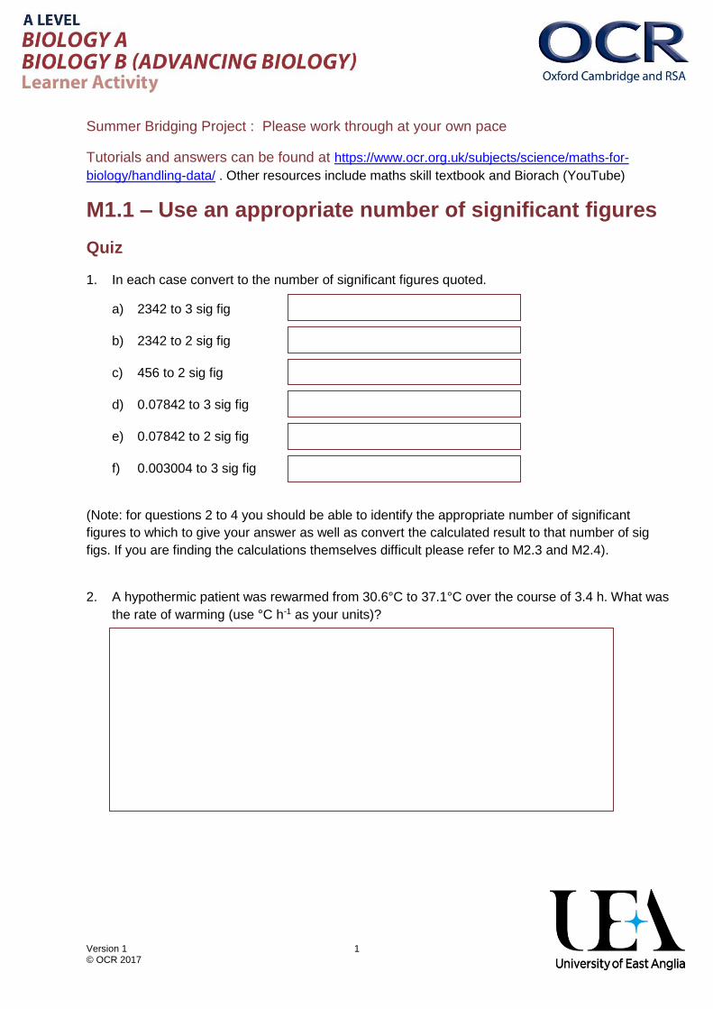
Version 1 1 © OCR 2017

Summer Bridging Project : Please work through at your own pace

Tutorials and answers can be found at https://www.ocr.org.uk/subjects/science/maths-for-

biology/handling-data/ . Other resources include maths skill textbook and Biorach (YouTube)

M1.1 – Use an appropriate number of significant figures

Quiz

1. In each case convert to the number of significant figures quoted.

a) 2342 to 3 sig fig

b) 2342 to 2 sig fig

c) 456 to 2 sig fig

d) 0.07842 to 3 sig fig

e) 0.07842 to 2 sig fig

f) 0.003004 to 3 sig fig

(Note: for questions 2 to 4 you should be able to identify the appropriate number of significant

figures to which to give your answer as well as convert the calculated result to that number of sig

figs. If you are finding the calculations themselves difficult please refer to M2.3 and M2.4).

2. A hypothermic patient was rewarmed from 30.6°C to 37.1°C over the course of 3.4 h. What was

the rate of warming (use °C h-1 as your units)?

Version 1 2 © OCR 2017

3. A willow coppice woodland in the UK has an area of 1.15 ha. (ha is the symbol for heactare

– an area of land equal to 10,000 m2). When the willow harvest is taken each year, and

dried, it yields 9 odt (oven-dry tonnes) of biomass. What is the productivity of the land (the

amount of biomass produced per unit area) in units of odt ha-1?

4. A model cell is made of visking tubing (partially permeable membrane) containing sucrose

solution and is immersed in distilled water. In 23.5 min the volume of the model cell

increases by 1.0 cm3 due to inflow of water by osmosis. What is the rate of osmosis in units

of cm3 min-1?

Version 1 3 © OCR 2017

M1.2 – Find arithmetic means

Quiz - calculate the mean:

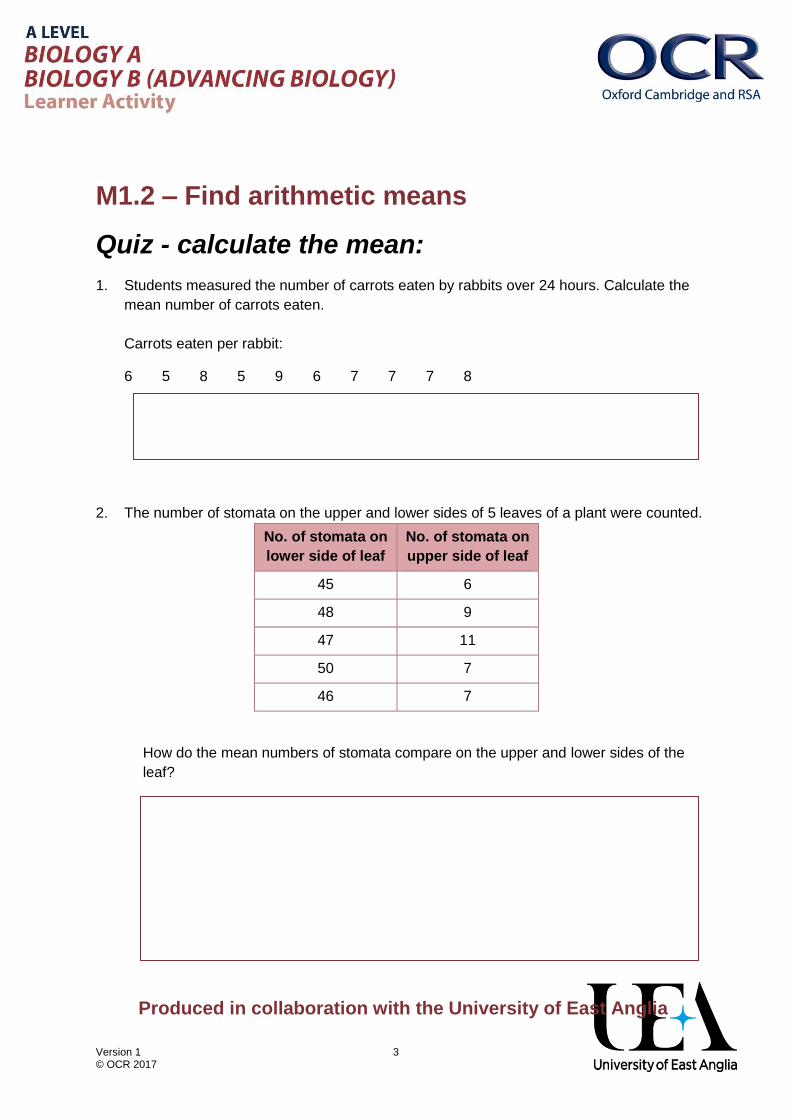
1. Students measured the number of carrots eaten by rabbits over 24 hours. Calculate the

mean number of carrots eaten.

Carrots eaten per rabbit:

6 5 8 5 9 6 7 7 7 8

2. The number of stomata on the upper and lower sides of 5 leaves of a plant were counted.

No. of stomata on

lower side of leaf

No. of stomata on

upper side of leaf

45 6

48 9

47 11

50 7

46 7

How do the mean numbers of stomata compare on the upper and lower sides of the

leaf?

Produced in collaboration with the University of East Anglia

Version 1 4 © OCR 2017

M1.3 – Construct and interpret frequency tables

and diagrams, bar charts and histograms

Quiz

For the below data sets:

a) Determine whether a histogram or bar chart is the more appropriate graph to plot with reasons.

b) Plot the graph.

1. Blood samples were taken from a group of patients and the frequency of blood groups is presented in the table below.

Blood group Frequency

A 40

B 10

AB 5

O 40

2. The ages of teenage boys and men attending at least one hour of gym class in a week were recorded. Process and present these data to show how the numbers doing this kind of exercise vary with age.

Age (years)

Age (years)

Age (years)

Age (years)

Age (years)

Age (years)

Age (years)

Age (years)

Age (years)

Age (years)

15.7 56.1 50.1 34.1 16.4 44.2 65.5 45.0 57.4 22.2

31.7 35.4 17.8 19.2 32.2 62.9 77.0 28.1 33.4 18.8

23.6 25.6 27.7 48.7 39.9 30.9 34.4 77.8 53.7 52.2

27.0 17.2 43.5 21.1 54.2 31.1 24.4 18.1 34.0 21.5

16.3 25.0 20.6 19.9 22.7 64.0 29.9 24.2 32.4 17.7

36.4 22.0 21.0 50.4 18.6 19.6 49.1 38.6 49.9 46.1

48.8 31.1 39.8 57.3 30.1 33.1 23.5 36.1 41.1 43.7

Version 1 5 © OCR 2017

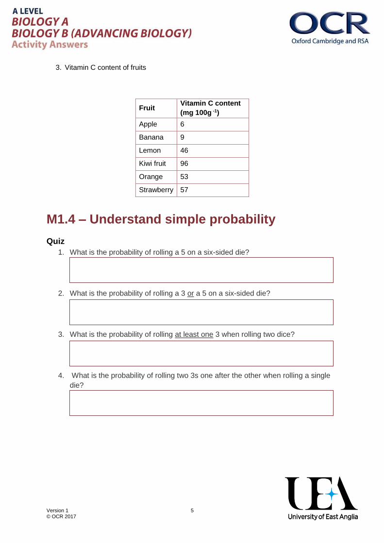
3. Vitamin C content of fruits

M1.4 – Understand simple probability

Quiz

1. What is the probability of rolling a 5 on a six-sided die?

2. What is the probability of rolling a 3 or a 5 on a six-sided die?

3. What is the probability of rolling at least one 3 when rolling two dice?

4. What is the probability of rolling two 3s one after the other when rolling a single

die?

Fruit Vitamin C content

(mg 100g -1)

Apple 6

Banana 9

Lemon 46

Kiwi fruit 96

Orange 53

Strawberry 57

Version 1 6 © OCR 2017

5. We have two cats where one is homozygous for alleles that produce a short tail

which is a recessive trait, while the other is homozygous for alleles that produce a

long tail which is dominant. With this knowledge we can make predictions about

the characteristics of any offspring produced when these two cats are bred

together.

A. What is the probability that offspring would inherit one copy of the short tail

allele?

B. What is the probability that offspring would have short tails?

Version 1 7 © OCR 2017

M1.5 – Understand the principles of sampling

as applied to scientific data

Quiz

1. I want to measure the change in distribution of green alga from the low tide mark to the

high tide mark. Should I use a random or non-random sampling method for choosing

where to place my quadrats?

2. You want to measure the distribution of flowers in a woodland. The woodland has been

divided up into 100 areas of 10 m2. You cannot measure them all and so have to choose

10 sampling points. Should you use random or non-random sampling?

3. If in the previous example 19 of the areas were identified as heavily waterlogged how

might stratified sampling be employed to improve our sampling technique?

4. A rock pool was sampled for species richness.

Calculate Simpsons Index of Diversity for this habitat using the formula:

𝐷 = 1 − ∑(𝑛

𝑁)2

Species Numbers

Common periwinkle 35

Dog whelk 41

Common limpet 8

Sea urchin 4

Top shells 24

Total (N)

Version 1 8 © OCR 2017

M1.6 – Understand the terms mean, mode

and median

Quiz

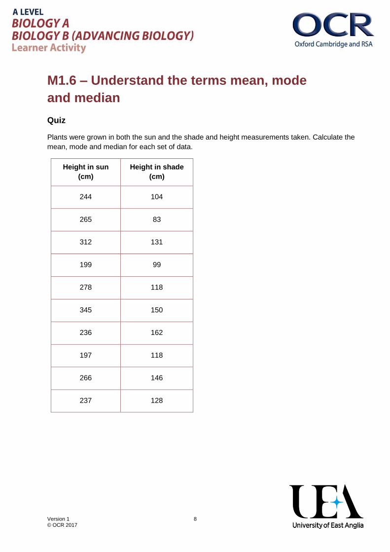
Plants were grown in both the sun and the shade and height measurements taken. Calculate the

mean, mode and median for each set of data.

Height in sun

(cm)

Height in shade

(cm)

244 104

265 83

312 131

199 99

278 118

345 150

236 162

197 118

266 146

237 128

Version 1 9 © OCR 2017

Height in sun (cm) Height in shade (cm)

Mean

Mode

Median

Numbers of mucus-secreting goblet cells were counted per colonic intestinal crypt in patients with

Crohn’s disease and healthy patients. Calculate the mean, mode and median for each set of data.

Number of goblet cells –

Crohn’s disease patients

Number of goblet cells –

Healthy patients

9 15

11 12

7 14

15 9

10 11

8 13

7 12

12 10

13 16

7 11

Crohn’s disease patients

Healthy patients

Mean

Mode

Median

Version 1 10 © OCR 2017

M1.7 – Use a scatter diagram to identify a

correlation between two variables

Quiz

1. Which of the following is/are appropriate to draw as scatterplots?

A. The mean horn length of two populations of African rhinos

B. The frequency of short-haired and long-haired cats from a cross of two long-haired

parents

C. The diameter of oak tree trunks and the average number of leaves per branch

D. The abundance of insects and the fledging weight of lapwing chicks.

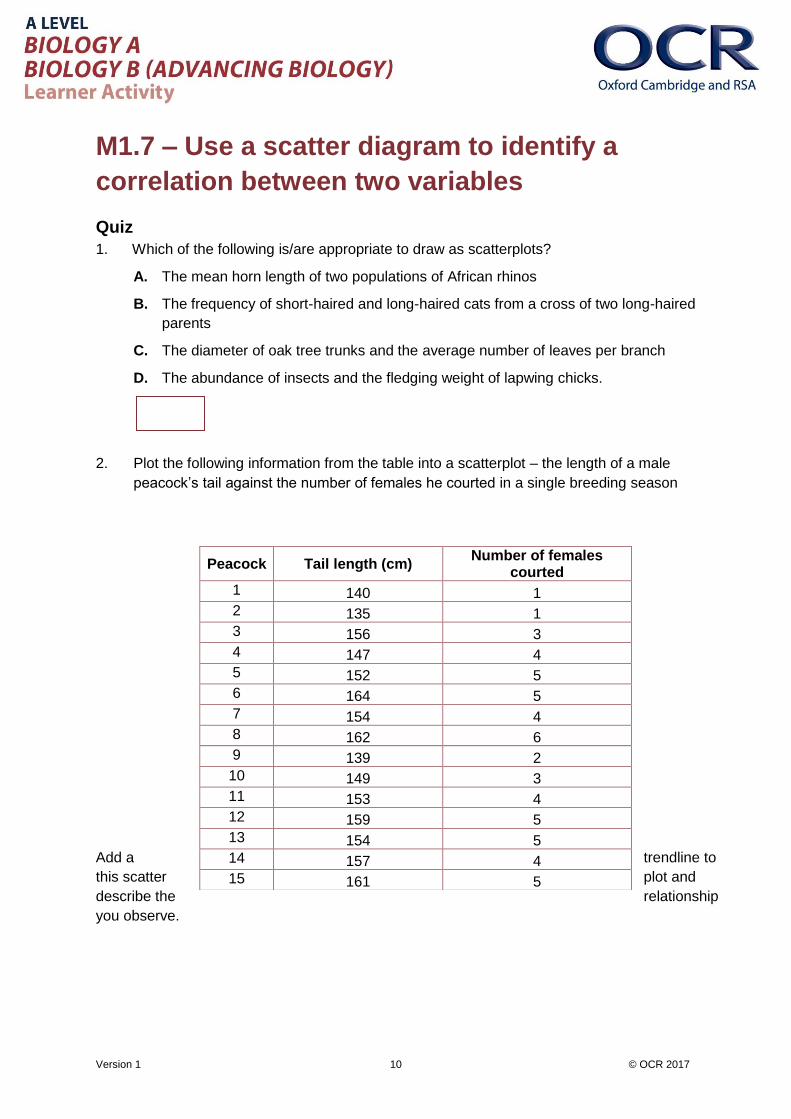
2. Plot the following information from the table into a scatterplot – the length of a male

peacock’s tail against the number of females he courted in a single breeding season

Add a trendline to

this scatter plot and

describe the relationship

you observe.

Peacock Tail length (cm) Number of females

courted

1 140 1

2 135 1

3 156 3

4 147 4

5 152 5

6 164 5

7 154 4

8 162 6

9 139 2

10 149 3

11 153 4

12 159 5

13 154 5

14 157 4

15 161 5

Version 1 11 © OCR 2017

3. Describe the relationship observed in this scatterplot charting the weight of female house

flies against the number of eggs laid per day.

0

20

40

60

80

100

120

140

160

180

0 1 2 3 4 5 6 7

Nu

mb

er

of

egg

s la

id p

er

day

Weight (mg)

Version 1 12 © OCR 2017

M1.8 Make order of magnitude calculations

Quiz

1 This is an electron micrograph of a mitochondrion. Its actual length is 5 μm. Calculate the magnification of the image.

B0000119 Credit Prof. R. Bellairs, Wellcome Images

TEM of a mitochondrion

A transmission electron micrograph of a mitochondrion in a chick embryo cell.

Collection: Wellcome Images

Copyrighted work available under Creative Commons Attribution only licence CC BY

4.0 http://creativecommons.org/licenses/by/4.0/

Version 1 13 © OCR 2017

2 This botanical illustration from about 250 years ago shows a banana plant. The image has a scale line where each division represents 30 cm. What is the magnification?

V0043033 Credit: Wellcome Library, London

Banana plant (Musa species): flowering and fruiting plant with stolons and separate floral segments and

sectioned fruit, also a description of the plant's growth, anatomical labels and a scale bar. Etching by G. D.

Ehret, c. 1742, after himself.

Version 1 14 © OCR 2017

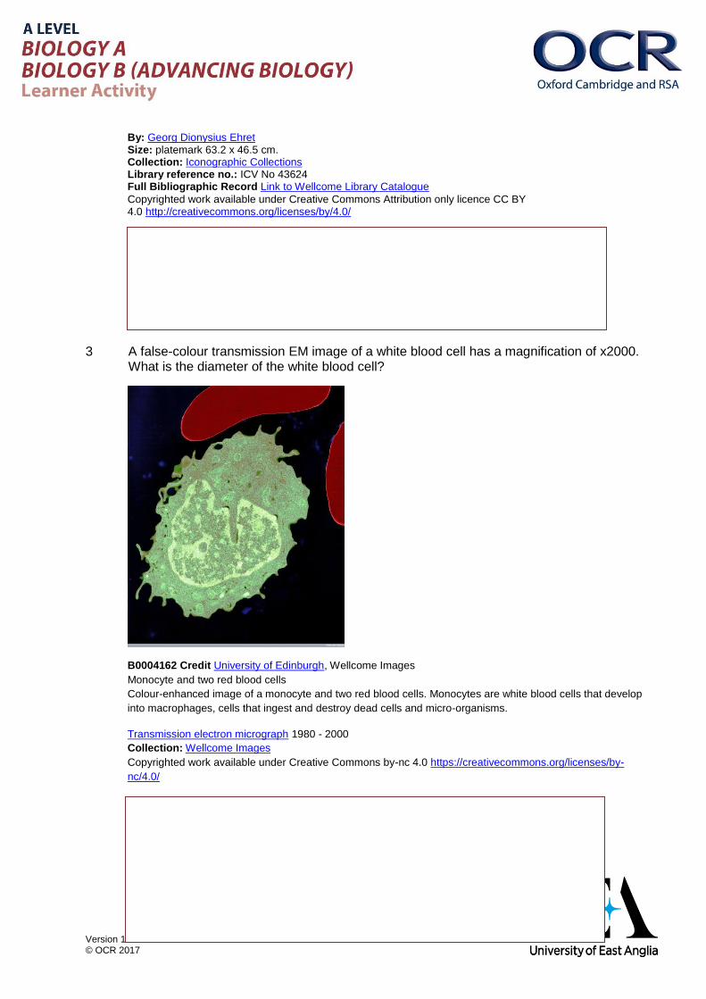
By: Georg Dionysius Ehret Size: platemark 63.2 x 46.5 cm. Collection: Iconographic Collections Library reference no.: ICV No 43624 Full Bibliographic Record Link to Wellcome Library Catalogue

Copyrighted work available under Creative Commons Attribution only licence CC BY 4.0 http://creativecommons.org/licenses/by/4.0/

3 A false-colour transmission EM image of a white blood cell has a magnification of x2000. What is the diameter of the white blood cell?

B0004162 Credit University of Edinburgh, Wellcome Images

Monocyte and two red blood cells

Colour-enhanced image of a monocyte and two red blood cells. Monocytes are white blood cells that develop

into macrophages, cells that ingest and destroy dead cells and micro-organisms.

Transmission electron micrograph 1980 - 2000

Collection: Wellcome Images

Copyrighted work available under Creative Commons by-nc 4.0 https://creativecommons.org/licenses/by-

nc/4.0/

Version 1 15 © OCR 2017

M1.9 – Select and use a statistical test

Quiz

4. We measured the mass of nine sample adult males in each of two separate populations of

elephants (A and B), and want to know if the means of the two populations are different.

Sample number

1 2 3 4 5 6 7 8 9

Population A mass of adult

male (kg) 6000 5590 6124 5800 5987 6020 5900 6143 5699

Population B mass of adult

male (kg) 4100 5900 4867 5010 5534 5321 5987 5350 5478

a) Calculate the means and standard deviations for the two populations

Version 1 16 © OCR 2017

b) Which statistical test is appropriate for testing the hypothesis that there is a

difference in the mean mass of adult male elephants between these two

populations?

c) Calculate whether there is a significant difference between these means

2. For which one or more of the following is a Spearman’s rank correlation coefficient the

appropriate statistical test to use?

A Comparing the relationship between grey seal pup size and fat reserves

B Comparing the frequency of different species of bluebell in a woodland

C Describing the relationship between the numbers of ladybirds and the numbers of

aphids in 10 different meadows

D Comparing the average growth of bacteria on two types of agar plate, where one has

been treated with penicillin

Version 1.1 17 © OCR 2019

3. Equal amounts of two types of the bacteria E.coli are mixed together in a volumetric flask, one

of these populations of E.coli is carrying an antibiotic resistance gene. The mixture is then

poured out onto agar plates that have been inoculated with penicillin and incubated for 24

hours. Based on previous experiments, when we count the bacteria, we expect there to be

twice as many colonies on the plate with the resistance gene as without. If we found 846

colonies on our plates the next day, and 432 of them carried the resistance marker, does this

differ significantly from our expected frequency?

Version 1.1 18 © OCR 2019

M1.10 – Understanding measures of dispersion

including standard deviation and range

Quiz

1. Below are the ages (in months) of Queen ants of the genus Cardiocondyla from two

geographically isolated populations. For each population a random sample of 11 queens

was taken and the ages recorded. Calculate the mean age and standard deviation for

queens from each population. Which of these two populations has the smallest standard

deviation?

Queen ant

1 2 3 4 5 6 7 8 9 10 11

Queen age in months

Population A

6 8 10 8 9 6 7 12 14 11 9

Population B

8 8 9 14 16 9 15 13 12 11 8

Version 1.1 19 © OCR 2019

2. The vertical jump height (mm) was measured of two separate populations (A & B) of fleas.

Below are two histograms of the distributions of jump heights in the two populations. Both

populations had a normal distribution around a common mean jump height of 100 mm.

Which population has the greatest standard deviation?

A)

B)

0

2

4

6

8

10

12

Fre

qu

en

cy

Vertical height (mm)

0

2

4

6

8

10

12

Fre

qu

en

cy

Vertical height (mm)

Version 1.1 20 © OCR 2019

M1.11 Identify uncertainties in measurements and

use simple techniques to determine uncertainty

when data are combined

Quiz

1. A microscope graticule allows fine-scale measurements to be made under a microscope. If

the graticule’s uncertainty is ± 0.5 µm, and a protozoan parasite Trypanosoma is measured

as 50 µm, calculate the percentage error for this measurement.

2. Cell cultures of the bacteria E. coli can be measured by a spectrophotometer to give an

accurate (to within 2%) reading of bacteria cm-3

A sample has been calculated as containing 3 * 109 bacteria cm-3

Calculate the absolute uncertainty of this measurement.

3. A plant shoot is measured for growth over a 5-day time period. Every morning it was

measured with a ruler an uncertainty of ±0.5 mm and the height recorded as show below.

Calculate the difference in height between days 1 and 5 and state the percentage error in

this measurement.

Day 1 2 3 4 5

Height (mm) 8 11 16 21 24

Document updates

v1.0 April 2017 Original version.

v1.1 June 2019 Changed how the word accuracy and uncertainty were used in

order to be in line with the ‘Language of measurement’

Version 1.1 21 © OCR 2019

Maths skills – M1 Handling data

M1.1 – Use an appropriate number of significant figures

Significant figures demonstrate a level of resolution and are important in all sorts of biological

contexts, when reporting experimental data and for any calculation. This means your answer can

only have the same number of significant figures as the piece of data with the lowest number of

significant figures. Reporting significant figures may involve rounding up (5 or above) or down (4 or

below). Be careful of zeros – any at the front of the number are not significant figures. However

zeros must be reported if they occur within or at the end of the number.

M1.2 – Find arithmetic means

The mean is calculated by adding together all the values and dividing by the number of values. As

a formula this is written as:

The calculated value for the mean can be quoted to the same number of decimal places as the

raw data or to one more decimal place.

M1.3 – Construct and interpret frequency tables and diagrams, bar charts and histograms

In biology you need to be able to understand and interpret frequency tables for a variety of

biological contexts. In addition, you must know the difference between histograms and bar charts,

when to use them, how to plot them and how to interpret them.

Below are key factors you need to consider when creating frequency tables, bar charts or

histograms:

Frequency tables Bar charts and histograms

Headings Title

Units Axes labels (with units)

Consistent use of decimal places Independent Variable on x axis

Dependent Variable on y axis

Plot data carefully

Graph is >50% of space available

Version 1 22 © OCR 2017

You also need to remember the important differences between histograms and bar charts:

Bar charts Histogram

Discrete independent

variable data

Continuous independent

variable data

Bars the same width Bar width may differ

Bars not touching Bars touch

Discrete data plotted with bar charts can only take specific values (there are no ‘in between’

values) and may include variables such as eye colour, species name, . On the other hand

continuous data is plotted using histograms for variables measured to a specified resolution such

as height, weight, and age.

For histograms you must make sure that the different category labels do not overlap as your data

cannot be in two different categories. Unlike bar charts, the width of bars in a histogram do not all

need to be the same. This is because it is the area of the bar that needs to be proportional to the

frequency. In situations where the class width of categories differ, you need to calculate the

frequency density, and plot these values on the y axis of your histogram.

M1.4 – Understand simple probability

Estimating probabilities is a fundamental part of working out the likelihood of an event occurring.

By understanding probabilities, we can make inferences about the results we are collecting and

draw conclusions. When an event is random, it does not mean that it is rare, just that it is

unpredictable. Probabilities allow us to predict the likelihood of an event occurring and identify

patterns that occur over time, even if we cannot predict the outcome of a single event.

M1.5 – Understand the principles of sampling as applied to scientific data

Sampling is a way of designing an experiment so that you can measure a representative part of a

population. Sampling can be random, where samples are taken in an unbiased way from the whole

population or system being studied, or non-random where samples are taken in a pre-defined

pattern.

Choosing whether to sample randomly or non-randomly depends on whether distribution is an

important part of the question, such as “how does the density of bluebells change as I move away

from the base of an oak tree”. This is a good example for non-random sampling. Otherwise

random sampling is a good way to avoid bias.

A community dominated by one or two species is considered to be less diverse than one in which

several different species have a similar abundance.

Simpson's Diversity Index is a measure of diversity which takes into account the number of

species present (species richness), as well as the relative abundance of each species (species

evenness). As species richness and evenness increase, so diversity increases.

Version 1 23 © OCR 2017

M1.6 – Understand the terms mean, median and mode

The mean, median and mode are all measures of central tendency and act as representative

values for the whole data set. The mean, mentioned previously in section M1.2, is the sum of the

data values divided by the number of data values. The median is the middle value of a data set

and requires the data to be put in ascending order first. The mode is the most frequently occurring

value and is usually the easiest to spot. Generally the mean is the most useful statistical measure,

except when there are outliers in the data when it may be more appropriate to use the median.

M1.7 – Use a scatter diagram to identify a correlation between two variables

Drawing a scatterplot allows you to see the relationship between two continuous variables. If a

relationship does exist between two continuous variables it can be described as a correlation: a

change in one variable tends to come with a change in the other variable. Correlations can be

linear or non-linear, positive or negative, and strong or weak. A combination of all three of these

terms can be used to describe a correlation e.g. a strong, positive, linear correlation.

Remember correlation does not imply causation!

M1.8 – Make order of magnitude calculations

Orders of magnitude are used to make approximate comparisons of size or quantity. If two

numbers have the same order of magnitude, they are about the same size. If two numbers differ

by one order of magnitude, one is about ten times larger than the other. If they differ by two orders

of magnitude, they differ by a factor of about 100, and so on.

The formula used to calculate magnification is:

objectrealofsize

imageofsizeionMagnificat

You can rearrange the formula to calculate any of the three unknowns, as long as you have the

other two. However for this to work you must make sure that both quantities/sizes are in the same

units.

M1.9 – Select and use a statistical test

Statistical tests allow us to draw conclusions about whether the results we have obtained are likely

to have come about by chance (the null hypothesis) or whether we have discovered a pattern or

process (the alternative hypothesis).

If the data we have gathered allows us to reject the null hypothesis, we do so at a certain

confidence level (usually 95%, also known as p=0.05). So when we reject the null hypothesis it

doesn’t mean our alternative hypothesis is certainly true, just that it is supported by the evidence

collected so far.

On the other hand, if the test we have carried out shows that we cannot reject the null hypothesis,

it does not mean the null hypothesis is true. It just means we have failed to disprove it with the

data under analysis.

Version 1 24 © OCR 2017

In order for our statistical tests to make meaningful inferences about biological systems and

processes, it is important that we use them appropriately.

t-tests can be used for comparing mean differences between groups, the Student’s t-test/ unpaired

t-test if they are two independent groups, or the paired t-test if it is the same group measured

before and after an event/manipulation.

Spearman’s rank correlation coefficient is used to look at relationships between two variables; is

there a consistent pattern where as one value rises the other also tends to rise/fall? Remember a

correlation can be positive or negative.

The chi squared test is used to identify whether frequencies of observations deviate from a pattern

of equal distribution, or another expected distribution.

The value generated by a statistical test can be used to estimate the probability that the results

you have obtained could have occurred by chance. To do this you must use the right table, for

example you must look in a t-value table when using a t-test. By using your test value and the

degrees of freedom you can look up the approximate p-value for your data.

The p-value is the probability from 0 to 1 that your results could have been obtained by chance

(i.e. that the null hypothesis is true), it is generally agreed that the threshold for rejecting the null

hypothesis is set at p<0.05.

M1.10 – Understand measures of dispersion, including standard deviation and range

Dispersion is the variability we find in our data. It can be measured in several different ways. The

simplest is the range, which looks at the difference between the highest and lowest scores in a

dataset. Although the range is easy to calculate, it is heavily influenced by extreme scores.

Another way of analysing dispersion is to calculate the standard deviation. This is the square root

of the average difference between the mean and each of the data points, it is a good measure of

the ‘fit’ of our data and allows us to make quantitative inferences about the population from which a

sample was taken.

M1.11 – Identify uncertainties in measurements and use simple techniques to determine uncertainty when data are combined

It is important to understand the difference between absolute and relative uncertainty.

Absolute uncertainty is a fixed value for any given measuring instrument.

Relative uncertainty is a value that changes dependent on the value of the measurement and the

absolute uncertainty.

When adding or subtracting measurements, you must add the absolute uncertainty values

together, to get an overall measure of the absolute uncertainty. From this absolute uncertainty you

can calculate the relative uncertainty or ‘percentage error’.

Version 1 25 © OCR 2017

Questions:

Questions M1.1

1) 0.30202 to 2 sig fig =

2) 0.675 to 2 sig fig =

3) 7.006 to 3 sig fig =

4) 6.001 to 2 sig fig =

Questions M1.2

Students had a competition to grow the tallest sunflower. Their measurements (in cm) are shown

below. Calculate the mean sunflower height.

102 95 89 110 79 82 94 87 93 81

Mean = …………………. cm

The lengths of mitochondria in a cell were measured (µm) and recorded. What is the mean

mitochondrion length?

2.4 3.4 4.5 7.0 6.8 5.6 5.7 7.0 5.9 6.1

Mean = ……………………….. µm

Version 1 26 © OCR 2017

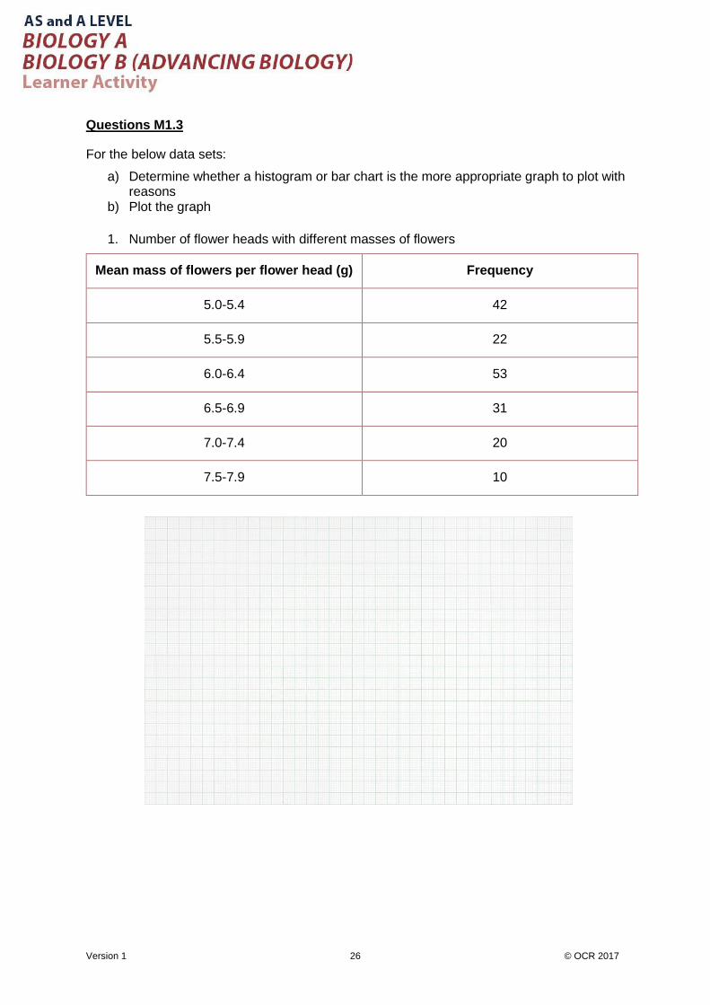
Questions M1.3

For the below data sets:

a) Determine whether a histogram or bar chart is the more appropriate graph to plot with reasons

b) Plot the graph

1. Number of flower heads with different masses of flowers

Mean mass of flowers per flower head (g) Frequency

5.0-5.4 42

5.5-5.9 22

6.0-6.4 53

6.5-6.9 31

7.0-7.4 20

7.5-7.9 10

Version 1 27 © OCR 2017

2. Number of flowers of different colours

Flower colour Frequency

White 46

Pink 92

Red 42

Questions M1.4

1. What is the probability of getting one ‘head’ and two ‘tails’ when three coins are tossed?

2. Two beetles with shiny wings are crossed. The resultant offspring are produced in a ratio of

3:1 shiny to dull wings. If we know a single gene controls this trait, what is the likely reason

for the appearance of the dull wing phenotype and why?

3. A Drosophila melanogaster cross is established with one parent homozygous for the wild

type vestigial allele and the other carrying one copy of the wild type allele and one copy of

the mutant allele.

a) What is the probability of offspring carrying at least one copy of the mutant allele?

b) What is the probability of offspring displaying the mutant vestigial phenotype?

Version 1 28 © OCR 2017

Questions M1.5

1. What are the two main approaches to sampling?

2. We wish to estimate the mean wing length in a population of Drosophila 10% of which

display the curly wing mutation. We aim to measure the wing lengths in 250 flies.

a) What method should be employed to take this sample?

b) What numbers of wildtype and curly wing flies should be included in this sample?

3. Two equal areas of the New Forest and the Forest of Dean were surveyed for numbers and

diversity of tree species.

For both locations calculate the Simpson’s Index of Diversity.

Which of the two forests has the higher biodiversity according to this survey?

Version 1 29 © OCR 2017

Question M1.6

Ecologists wanted to compare the number of buttercups and dandelions in a field. Using quadrats

they counted the numbers of each plant in 10 randomly selected 1 m2 areas. Calculate and

compare the mean, median and modes for each data set. Which is the most appropriate statistical

measure to report for each data set and why?

Number of buttercups Number of dandelions

9 18

15 19

58 16

12 22

10 21

13 16

15 20

11 17

14 20

15 72

Numbers

Species New Forest Forest of Dean

English oak 35 30

Ash 52 48

Beech 59 74

Birch 25 36

Sweet chestnut 5 0

Yew 3 2

Version 1 30 © OCR 2017

Questions M1.7

1. The male gray tree frog produces mating calls at regular intervals, but this interval

frequency is thought to be affected by the air temperature. Plot the data collected, add a

trendline and describe the relationship observed

Male call interval (s)

Temperature (°C)

2 16

4 26

2 18

3 20

3 24

4 19

6 32

3 29

6 30

5 28

3 21

2 16

2 23

1 11

1 16

3 19

2 11

5 26

3 19

5 27

2 12

1 11

2 17

2 11

4 27

3 22

4 18

1 11

1 11

Version 1 31 © OCR 2017

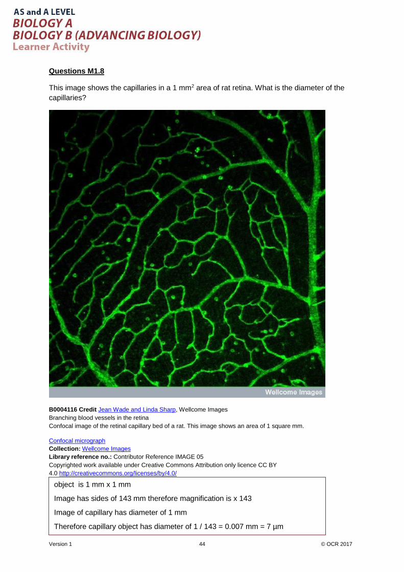
Questions M1.8

This image shows the capillaries in a 1 mm2 area of rat retina. What is the diameter of the

capillaries?

B0004116 Credit Jean Wade and Linda Sharp, Wellcome Images

Branching blood vessels in the retina

Confocal image of the retinal capillary bed of a rat. This image shows an area of 1 square mm.

Confocal micrograph

Collection: Wellcome Images

Library reference no.: Contributor Reference IMAGE 05

Copyrighted work available under Creative Commons Attribution only licence CC BY

4.0 http://creativecommons.org/licenses/by/4.0/

Version 1 32 © OCR 2017

Questions M1.9

1. We are interested in determining whether there is an effect of the addition of nitrate

fertiliser on the mean height of Brassica crops. Two fields are treated identically apart from

the use of fertiliser on one but not the other. Mature plants from each field were then

chosen at random and the heights measured.

a) Generate a null and alternative hypothesis on the effect of fertiliser on crop growth

b) The sample data collected from the two fields is as follows. Calculate the t-value and

determine if there is a significant difference between the two treatments

Height of crop when nitrate

fertiliser added (cm) n = 23

Height of crop when no fertiliser added (cm)

n = 24

Mean 142 101

Standard deviation 23 18

B

B

A

A

BA

n

s

n

s

xxt

22

24

324

23

529

101142

t = 6.8

Version 1 33 © OCR 2017

2. The average time between the production of two RNA transcripts from the same strand of

DNA in a cell is known as the ‘synthesis time’, we wish to know whether products that take

longer to be synthesised by a cell also last longer or whether they are targeted for

degradation at the same rate. To do this the “half-life” (the time needed for half of a batch

of mature RNAs to degrade) was measured for each transcript separately.

RNA molecule Synthesis time (s) “Half-life”(s)

1 240 98

2 230 203

3 1000 180

4 78 226

5 194 162

6 182 173

7 675 156

8 345 146

9 982 186

10 112 178

a) Produce null and alternative hypotheses for this experiment

b) What is the rs value for this data – is this a significant relationship?

c) Describe the results in terms of your hypotheses

Version 1 34 © OCR 2017

RNA molecule

Synthesis time (s)

Rank “Half-life”(s)

Rank Difference in rank

Difference squared

1 240 5 98 10 5 25

2 230 6 203 2 4 16

3 1000 1 180 4 3 9

4 78 10 226 1 9 81

5 194 7 162 7 0 0

6 182 8 173 6 2 4

7 675 3 156 8 5 25

8 345 4 146 9 5 25

9 982 2 186 3 1 1

10 112 9 178 5 4 16

22.0990

12121

)110(10

20261

)1(

61

22

2

nn

drs

Version 1 35 © OCR 2017

Questions M1.10

1. Here is a dataset of the cell sizes of a sample from a population of the single-celled

eukaryote Paramecium bursaria

Sample 1 2 3 4 5 6 7 8 9 10

Size (µm)

80 150 95 110 210 140 97 101 85 134

a) State the interval that covers one standard deviation above and one standard

deviation below the mean.

b) Any scores which lie more than three standard deviations above or below the mean

could be considered extreme scores, are there any scores which fit this criterion?

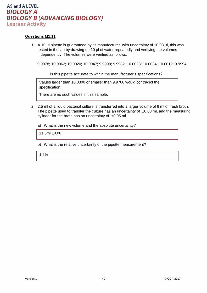
Questions M1.11

1. A 10 µl pipette is guaranteed by its manufacturer with uncertainty of ±0.03 µl, this was

tested in the lab by drawing up 10 µl of water repeatedly and verifying the volumes

independently. The volumes were verified as follows:

9.9978; 10.0062; 10.0020; 10.0047; 9.9998; 9.9982; 10.0023; 10.0034; 10.0012; 9.9994

Is this pipette accurate to within the manufacturer’s specifications?

Version 1 36 © OCR 2017

2. 2.5 ml of a liquid bacterial culture is transferred into a larger volume of 9 ml of fresh broth.

The pipette used to transfer the culture has an uncertainty of ±0.03 ml, and the measuring

cylinder for the broth has an uncertainty of ±0.05 ml.

a) What is the new volume and the absolute uncertainty?

b) What is the relative uncertainty of the pipette measurement?

Version 1 37 © OCR 2017

Answers:

Questions M1.1

1) 0.30202 to 2 sig fig =

2) 0.675 to 2 sig fig =

3) 7.006 to 3 sig fig =

4) 6.001 to 2 sig fig =

Questions M1.2

Students had a competition to grow the tallest sunflower. There measurements (in cm) are shown

below. Calculate the mean sunflower height.

102 95 89 110 79 82 94 87 93 81

Mean = 912/10 = 91.2 cm

The lengths of mitochondria in a cell were measured (µm) and recorded. What is the mean

mitochondria length?

2.4 3.4 4.5 7.0 6.8 5.6 5.7 7.0 5.9 6.1

52/9 = 5.77778

Mean = 5.78 (or 5.8) µm

0.30

0.68

7.01

6.0

Version 1 38 © OCR 2017

Questions M1.3

For the below data sets:

a) Determine whether a histogram or bar chart is the more appropriate graph to plot with reasons

b) Plot the graph

3. Number of flower heads with different masses of flowers

Mean mass of flowers per flower head (g) Frequency

5.0-5.4 42

5.5-5.9 22

6.0-6.4 53

6.5-6.9 31

7.0-7.4 20

7.5-7.9 10

Histogram – continuous data

Version 1 39 © OCR 2017

3/8

The emergence of a new phenotype suggests that the parents were both

carrying a recessive allele for dull wings. 3:1 is the expected ratio that would

result from such a cross – other theorised parental combinations of alleles for a

single gene trait would not produce the ratio of offspring observed.

0.5

4. Number of flowers of different colours

Flower colour Frequency

White 46

Pink 92

Red 42

Bar chart – discrete data

Questions M1.4

1. What is the probability of getting one ‘head’ and two ‘tails’ when three coins are tossed?

2. Two beetles with shiny wings are crossed. The resultant offspring are produced in a ratio of

3:1 shiny to dull wings. If we know a single gene controls this trait, what is the likely reason

for the appearance of the dull wing phenotype and why?

3. A Drosophila melanogaster cross is established with one parent homozygous for the wild

type vestigial allele and the other carrying one copy of the wild type allele and one copy of

the mutant allele.

a. What is the probability of offspring carrying at least one copy of the mutant allele?

0

10

20

30

40

50

60

70

80

90

100

White Pink Red

Nu

mb

er

of

flo

we

rs

Flower colour

Number of flowers of different colours

Version 1 40 © OCR 2017

0

Random and non-random

Stratified random sampling

25 curly wings and 225 wildtype

The New forest has a greater D value – therefore the higher biodiversity

b. What is the probability of offspring displaying the mutant vestigial phenotype?

Questions M1.5

1. What are the two main approaches to sampling?

2. We wish to estimate the mean wing length in a population of Drosophila 10% of which

display the curly wing mutation. We aim to measure the wing lengths in 250 flies.

a) What method should be employed to take these samples?

b) What numbers of wildtype and curly wing flies should be included in this sample?

3. Two equal areas of the New Forest and the Forest of Dean were surveyed for numbers and

diversity of tree species. For both locations calculate the Simpson’s Index of Diversity.

Which of the two forests has the higher biodiversity according to this survey?

Question M1.6:

Numbers

Species New Forest Forest of Dean

English oak 35 30

Ash 52 48

Beech 59 74

Birch 25 36

Sweet chestnut 5 0

Yew 3 2

Simpson’s Index 0.75 0.72

Version 1 41 © OCR 2017

Buttercups Dandelions Mean 17.2 24.1

Median 13.5 19.5 Mode 15 16

There are outliers in both data sets therefore the median is more representative

to report.

Ecologists wanted to compare the number of buttercups and dandelions in a field. Using quadrats

they counted the numbers of each plant in 10 randomly selected 1 m2 areas. Calculate and

compare the mean, median and modes for each data set. Which is the most appropriate statistical

measure to report for each data set and why?

Number of buttercups Number of dandelions

9 18

15 19

58 16

12 22

10 21

13 16

15 20

11 17

14 20

15 72

Version 1 42 © OCR 2017

Questions M1.7

2. The male gray tree frog produces mating calls at regular intervals, but this interval

frequency is thought to be affected by the air temperature. Plot the data collected add a

trendline and describe the relationship observed

Male call interval (s)

Temperature (°C)

2 16

4 26

2 18

3 20

3 24

4 19

6 32

3 29

6 30

5 28

3 21

2 16

2 23

1 11

1 16

3 19

2 11

5 26

3 19

5 27

2 12

1 11

2 17

2 11

4 27

3 22

4 18

1 11

1 11

Version 1 43 © OCR 2017

A strong positive correlation.

0

5

10

15

20

25

30

35

40

0 1 2 3 4 5 6 7

Tem

p (

C)

Male calling interval (s)

Version 1 44 © OCR 2017

object is 1 mm x 1 mm

Image has sides of 143 mm therefore magnification is x 143

Image of capillary has diameter of 1 mm

Therefore capillary object has diameter of 1 / 143 = 0.007 mm = 7 µm

Questions M1.8

This image shows the capillaries in a 1 mm2 area of rat retina. What is the diameter of the

capillaries?

B0004116 Credit Jean Wade and Linda Sharp, Wellcome Images

Branching blood vessels in the retina

Confocal image of the retinal capillary bed of a rat. This image shows an area of 1 square mm.

Confocal micrograph

Collection: Wellcome Images

Library reference no.: Contributor Reference IMAGE 05

Copyrighted work available under Creative Commons Attribution only licence CC BY

4.0 http://creativecommons.org/licenses/by/4.0/

Version 1 45 © OCR 2017

Null – There is no effect of fertiliser application on the mean height of Brassica

crops

Alternative – There is an effect of fertiliser application on the mean height of

Brassica crops or The Brassica crop exposed to fertiliser will be taller than the

brassica not exposed to fertiliser.

Should apply the Student’s t-test – two independent groups

Questions M1.9

1. We are interested in determining whether there is an effect of the addition of nitrate

fertiliser on the mean height of Brassica crops. Two fields are treated identically apart from

the use of fertiliser on one but not the other. Mature plants from each field were then

chosen at random and the heights measured.

a) Generate a null and alternative hypothesis on the effect of fertiliser on crop growth

b) The sample data collected from the two fields is as follows. Calculate the t-value and

determine if there is a significant difference between the two treatments

Height of crop when nitrate

fertiliser added (cm) n = 23

Height of crop when no fertiliser added (cm)

n = 24

Mean 142 101

Standard deviation 23 18

B

B

A

A

BA

n

s

n

s

xxt

22

24

324

23

529

101142

t = 6.8

Version 1 46 © OCR 2017

t = 6.8

degrees of freedom = n1 - 1 + n2 - 1 = 45

6.8 is well in excess of the threshold for p=0.05 and indeed for p=0.01.

Therefore there is a significant difference in the sample means and we can

reject the null hypothesis.

The crop treated with nitrate fertiliser grew taller.

2. The average time between the production of two RNA transcripts from the same strand of

DNA in a cell is known as the ‘synthesis time’, we wish to know whether products that take

longer to be synthesised by a cell also last longer or whether they are targeted for degradation

at the same rate. To do this the “half-life” (the time needed for half of a batch of mature RNAs

to degrade) was measured for each transcript separately.

RNA molecule Synthesis time (s) “Half-life”(s)

1 240 98

2 230 203

3 1000 180

4 78 226

5 194 162

6 182 173

7 675 156

8 345 146

9 982 186

10 112 178

Version 1 47 © OCR 2017

Null – There is no correlation between synthesis time and half-life for RNA

production. Alternative – The synthesis time correlates with the half-life of RNA

molecules

Sum of difference squared = 202

a) Produce null and alternative hypotheses for this experiment

b) What is the rs value for this data – is this a significant relationship?

c) Describe the results in terms of your hypotheses

RNA molecule

Synthesis time (s)

Rank “Half-life”(s)

Rank Difference in rank

Difference squared

1 240 5 98 10 5 25

2 230 6 203 2 4 16

3 1000 1 180 4 3 9

4 78 10 226 1 9 81

5 194 7 162 7 0 0

6 182 8 173 6 2 4

7 675 3 156 8 5 25

8 345 4 146 9 5 25

9 982 2 186 3 1 1

10 112 9 178 5 4 16

22.0990

12121

)110(10

20261

)1(

61

22

2

nn

drs

Version 1 48 © OCR 2017

rs = -0.22

We have a negative correlation coefficient, suggesting the possibility of a

negative correlation between synthesis time and half-life. However, is this

significant or just due to chance? We check the critical value table (ignoring the

negative sign in our result)

The critical value for the Spearman’s rank correlation coefficient at p= 0.05

where n is 10 is 0.6485

The calculated rs value ( 0.22, ignoring the negative) is less than the critical

value so there is no significant correlation

We have failed to reject the null hypothesis that there is no relationship between

synthesis time and half-life of RNA molecules.

80.7-159.7 um

No

Questions M1.10

1. Here is a dataset of the cell sizes of a sample from a population of the single-celled

eukaryote Paramecium bursaria

Sample 1 2 3 4 5 6 7 8 9 10

Size (um)

80 150 95 110 210 140 97 101 85 134

a) State the interval that covers one standard deviation above and one standard

deviation below the mean.

b) Any scores which lie more than three standard deviations above or below the mean

could be considered extreme scores, are there any scores which fit this criterion?

Version 1 49 © OCR 2017

Values larger than 10.0300 or smaller than 9.9700 would contradict the

specification.

There are no such values in this sample.

11.5ml ±0.08

1.2%

Questions M1.11

1. A 10 µl pipette is guaranteed by its manufacturer with uncertainty of ±0.03 µl, this was

tested in the lab by drawing up 10 µl of water repeatedly and verifying the volumes

independently. The volumes were verified as follows:

9.9978; 10.0062; 10.0020; 10.0047; 9.9998; 9.9982; 10.0023; 10.0034; 10.0012; 9.9994

Is this pipette accurate to within the manufacturer’s specifications?

2. 2.5 ml of a liquid bacterial culture is transferred into a larger volume of 9 ml of fresh broth.

The pipette used to transfer the culture has an uncertainty of ±0.03 ml, and the measuring

cylinder for the broth has an uncertainty of ±0.05 ml.

a) What is the new volume and the absolute uncertainty?

b) What is the relative uncertainty of the pipette measurement?

Version 1 50 © OCR 2017

Document updates

v1.0 April 2017 Original version.

v1.1 June 2019 Changed how the word accuracy, resolution and uncertainty were

used in order to be in line with the ‘Language of measurement’.

Clarification on the Student’s t-test.

We’d like to know your view on the resources we produce. By clicking on ‘Like’ or ‘Dislike’ you can help us to ensure that our resources

work for you. When the email template pops up please add additional comments if you wish and then just click ‘Send’. Thank you.

If you do not currently offer this OCR qualification but would like to do so, please complete the Expression of Interest Form which can

be found here: www.ocr.org.uk/expression-of-interest

Looking for a resource? There is now a quick and easy search tool to help find free resources for your qualification:

www.ocr.org.uk/i-want-to/find-resources/

OCR Resources: the small print

OCR’s resources are prvided to support the delivery of OCR qualifications, but in no way constitute an endorsed teaching method that is required by the Board, and the decision to

use them lies with the individual teacher. Whilst every effort is made to ensure the accuracy of the content, OCR cannot be held responsible for any errors or omissions within

these resources.

© OCR 2019 - This resource may be freely copied and distributed, as long as the OCR logo and this message remain intact and OCR is acknowledged as the originator of this work.

OCR acknowledges the use of the following content: M1.8:: B0004116 Credit Jean Wade and Linda Sharp, Wellcome Images, Copyrighted work available under Creative Commons

Attribution only licence CC BY 4.0 htp://creativecommons.org/licenses/by/4.0/

Please get in touch if you want to discuss the accessibility of resources we offer to support delivery of our qualifications: resources.feedback@ocr.org.uk

Produced in collaboration with the University of East Anglia

This resource has been produced as part of our free A Level teaching and learning support package. All the A Level teaching and

learning resources, including delivery guides, topic exploration packs, lesson elements and more are available on the qualification

webpages.

If you are looking for examination practice materials, you can find the Sample Assessment Materials (SAMs) on the qualification

webpages: Biology A / Biology B