M-PERT: manual project-duration estimation technique for ...

M-PERT: manual project-duration estimation technique for teaching scheduling basics

Article

Accepted Version

Ballesteros-Pérez, P. (2017) M-PERT: manual project-duration estimation technique for teaching scheduling basics. Journal of Construction Engineering and Management, 143 (9). 04017063. ISSN 0733-9364 doi: https://doi.org/10.1061/(ASCE)CO.1943-7862.0001358 Available at http://centaur.reading.ac.uk/69858/

It is advisable to refer to the publisher’s version if you intend to cite from the work. See Guidance on citing .Published version at: http://ascelibrary.org/doi/10.1061/%28ASCE%29CO.1943-7862.0001358

To link to this article DOI: http://dx.doi.org/10.1061/(ASCE)CO.1943-7862.0001358

Publisher: American Society of Civil Engineers

All outputs in CentAUR are protected by Intellectual Property Rights law, including copyright law. Copyright and IPR is retained by the creators or other

http://centaur.reading.ac.uk/71187/10/CentAUR%20citing%20guide.pdf

copyright holders. Terms and conditions for use of this material are defined in the End User Agreement .

www.reading.ac.uk/centaur

CentAUR

Central Archive at the University of Reading

Reading’s research outputs online

http://www.reading.ac.uk/centaur

http://centaur.reading.ac.uk/licence

THANKS FOR DOWNLOADING THIS PAPER.

This is a post-refereeing version of a manuscript published by the ASCE.

Please, in order to cite this paper properly:

Ballesteros-Pérez, P. (2017) “M-PERT. A manual project duration estimation

technique for teaching scheduling basics.” Journal of Construction Engineering and

Management. In press.

http://dx.doi.org/10.1061/(ASCE)CO.1943-7862.0001358

The authors recommend going to the publisher’s website in order to access the full paper.

If this paper helped you somehow in your research, feel free to cite it.

1

M-PERT. A manual project duration estimation technique 1

for teaching scheduling basics 2

Pablo Ballesteros-Pérez, Ph.D. 3

Lecturer. School of Construction Management and Engineering. University of Reading, 4

Whiteknights, Reading RG6 6AW, United Kingdom. E-mail: [email protected] 5

ABSTRACT 6

The Program Evaluation and Review Technique (PERT) has become a classic Project 7

Management tool for estimating project duration when the activities have uncertain durations. 8

However, despite its simplicity and widespread adoption, the original PERT, in neglecting 9

the merge event bias, significantly underestimated the duration average and overestimated the 10

duration variance of real-life projects. To avoid these and other shortcomings, many authors 11

have worked over the last 60 years at producing interesting alternative PERT extensions. This 12

paper proposes joining the most relevant of those to create a new reformulated PERT, named 13

M-PERT. 14

M-PERT is quite accurate when estimating real project duration, while also allowing for a 15

number of interesting network modelling features the original PERT lacked: probabilistic 16

alternative paths, activity self-loops, minima of activity sets and correlation between 17

activities. However, unlike similar scheduling methods, M-PERT allows manual calculation 18

through a recursive merging procedure that downsizes the network until the last standing 19

activity represents the whole (or remaining) project duration. Hence, M-PERT constitutes an 20

attractive tool for teaching scheduling basics to engineering students in a more intuitive way, 21

with or without the assistance of computer-based simulations or software. One full case study 22

will also be proposed and future research paths suggested. 23

KEYWORDS 24

Scheduling, PERT; GERT; Stochastic Network Analysis; Project duration. 25

2

Introduction 26

In 1959, an Operations Research team formed by D.G. Malcom, J.H. Roseboom and C.E. 27

Clark from the company Booz, Allen and Hamilton in Chicago, along with W. Fazar, from 28

the US Navy Special Projects Office in Washington, published a technique for measuring and 29

controlling the progress of the Polaris Fleet Ballistic Missile (FBM) program (Malcolm et al. 30

1959). This technique was initially named the Program Evaluation Research Task and later 31

renamed the Program Evaluation and Review Technique (PERT). It has become one of the 32

most popular Project Management (PM) scheduling tools since then. 33

The initial idea was to provide the project manager with an integrated and quantitative 34

management methodology that allowed him/her to evaluate ‘(a) [the] progress to date and 35

[the] outlook for accomplishing the objectives of the FBM program, (b) [the] validity of 36

established plans and schedules for accomplishing the program objectives, and (c) [the] 37

effects of changes proposed in established plans’ (Malcolm et al., 1959, p.646). These three 38

aims were quite ambitious indeed, and despite one imagining PERT doing all of these with a 39

leap of faith, what PERT actually and basically does is to estimate the probabilistic duration 40

of any project or the remaining part of a project when the activities have uncertain (not 41

deterministic) durations. Also, PERT can be implemented for cost estimation purposes with 42

some technical variations (e.g. (Asmar et al. 2011)); however, for the sake of clarity we will 43

just deal with the time dimension in this paper. 44

In its favor, this technique is very easy to implement and was the first of its kind for 45

dealing with projects whose activity durations are modeled by probability distributions, or 46

Stochastic Network Analysis (SNA) as it known as nowadays. Against it, the procedure 47

proposed by PERT underestimates the project duration when there are multiple parallel paths, 48

which unfortunately is the norm in construction projects. Indeed, the authors were aware of 49

this shortcoming since they very briefly mentioned in the original paper that ‘this 50

3

simplification gives biased estimates such that the estimated expected time of events are 51

always too small’ (Malcolm et al. 1959). Two publications by C.E. Clark indeed followed the 52

publication of PERT (Clark 1961, 1962), but the solution proposed was not easy to 53

implement, so it opened interesting avenues of research for the scientific community that 54

have continued to this day, mostly in the Operations Research discipline. 55

Since the inception of PERT almost 60 years ago, the number of fields in which this 56

technique has been applied has been quite varied. It is not only applied to military, research & 57

development and civil engineering projects as was originally intended (Stauber et al. 1959), 58

but also to fields as diverse as medicine (e.g. Woolf et al. (1968)), exports (e.g. Tatterson 59

(1974)), contracting (e.g. Mummolo (1997)) and rural development (e.g. Tavares (2002)), to 60

cite just a few. In fact, its reach and application are virtually unlimited since it is useful for 61

any project duration estimation purposes where activities have non-deterministic durations. 62

However, another collateral problem has been that despite PERT being a celebrated PM 63

technique, it also probably is one of the most widely misunderstood. In particular, many 64

engineering and scheduling students, as well as professionals, still think that PERT is either a 65

type of network representation, as one of the first versions of the Project Management Body 66

of Knowledge (PMBoK) pointed out explicitly (PMI 1996), or that it is just a three-point time 67

and/or cost estimation technique (PMI 2008). The latter misrepresentation is the consequence 68

of the second half of the PERT method, which deals with calculating the expected project 69

duration and its variance by means of critical path project activities, being left out of this 70

publication. 71

The purpose of this paper is to update PERT and propose a newly redefined technique 72

named M-PERT, which deals with the most relevant shortcoming of the original technique 73

(the merge event bias), allows manual calculation, and adds a series of new interesting 74

features that the original technique lacked. M-PERT will allow the modelling of real-life 75

4

projects far more representatively and help scheduling students to understand more intuitively 76

basic concepts of scheduling when activities have uncertain durations. 77

The number of PERT-related publications might be counted in the thousands nowadays, 78

so we cannot reference them all. Instead, as in any other mature fields, we will undertake a 79

systematic review of the most relevant sources that have shaped this new technique. This 80

systematic review will be presented in the Background section under three thematic 81

subsections. Then, an outline of the model will be presented followed by an application in the 82

M-PERT outline and Case study sections. A Results section will gather the application 83

outcomes while comparing the accuracy improvements achieved, whereas a final and brief 84

Discussions and conclusions section will summarize the most important aspects and possible 85

research directions for the model proposed. 86

87

Background 88

An overview of PERT and its limitations 89

In a nutshell, PERT is a scheduling tool that is applied in two stages. First, after 90

identifying all the activities involved in a project and stating their precedence relationships, 91

the first stage comprises modelling their probable durations. For that purpose, the original 92

PERT authors proposed a three-point estimation procedure. The user (or another expert on 93

hand) is asked to state the Optimistic (O), most Likely (L) and Pessimistic (P) durations that 94

each activity is foreseen to have before those activities take place. Then, the mean duration 95

(μ) and the standard deviation (σ) from each activity are calculated by using these three 96

duration estimates (O, L and P) by means of these straightforward expressions: 97

( ) 64 PLO ++= (1) 98

( ) 6OP= (2) 99

5

With the values of μ and σ for each activity, a Beta distribution which varies between 100

[O, P] is fitted for modelling the activity duration. However, despite the highly controversial 101

and still ongoing debate about the accuracy of both the three-point estimate procedure and the 102

choice of the Beta distribution to model the activity durations, the PERT method is only 103

interested in the μ and σ values of each activity for the second stage of the application. This 104

second stage of PERT (not mentioned by any Project Management standard) comprises: (a) 105

identifying the activities that are in the critical path, and (b) assuming that the Project 106

duration mean (μp) and the standard deviation (σp) are equal: 107

=pathcriticaliip (3) 108

=pathcriticaliip2 (4) 109

Now, if the project scheduler wants to know what the probabilities of ending a project in 110

X days are, he/she just needs to know that the project total duration is supposed to be 111

following a Normal distribution with mean μp and standard deviation σp. Then, the specific 112

probability of X happening can be calculated by means of either the mathematical expressions 113

of the cumulative Normal distribution, by resorting to a spreadsheet or, when the calculations 114

are made by hand, by standardizing the project duration as in Equation 5 and then looking up 115

the cumulative probability value of z in a standard Normal table. 116

( ) ppXz = (5) 117

This is the essence of the PERT method. The logical lack of trust displayed by the 118

research community since PERT was published has manifested itself as a determination to 119

see what kind of errors are involved by implementing it. In this regard, MacCrimmon and 120

Ryavec (1964) broke down PERT into every possible piece and developed the most thorough 121

analytical review that anyone has made of PERT since its publication. This piece of research 122

6

was actually outsourced by the US Air Force to the Rand Corporation due to the consistent 123

and systematic errors that PERT was evidencing in their project forecasts, and they divided 124

their memorandum into two main sections. In the first section, they studied the activity 125

duration-level errors, that is, ‘(1) the assumption of the Beta distribution, (2) imprecise time 126

estimates, and (3) the assumption of the standard deviation (one-sixth of the range) and the 127

approximation formula for calculating the mean time’ (MacCrimmon and Ryavec 1964). The 128

second section checked the accuracy of the project duration mean, variance and the (Normal) 129

probability statements. 130

The results summary from the first section was that using the three-point estimates could 131

cause a range estimation error of between 10% and 20% of the range [O, P], but, despite the 132

error of estimation of the mean (µ) and standard deviation (σ) being likely to be bigger (from 133

15% to 30%), a degree of cancellation was expected to occur depending on the network. 134

Indeed, there is generally a high degree of cancellation as will be proven later. But the other 135

noteworthy statement that the authors made at that time was that, to a certain extent, it was 136

pointless having a discussion about what the right kind of distribution is – Beta or another – 137

for modelling an activity duration. Indeed, they reinforced this idea by saying that if PERT 138

had used triangular distributions instead of Beta distributions, their analysis would have given 139

almost identical results (MacCrimmon and Ryavec 1964). A recent study only focusing on 140

determining the importance of the specific distribution selection in PERT also supported this 141

claim and stated that the maximum deviation by using alternative distributions in the project 142

duration an estimation is generally well below 10% (Hajdu and Bokor 2014). 143

Nevertheless, the results from the second section of the PERT model analysis evidenced 144

the real problem. They confirmed that unless there is one clear dominant critical path (a chain 145

of activities whose total duration is significantly longer than the second longest path), the 146

PERT-calculated mean (equation 3) will be biased optimistically (underestimating the real 147

7

project duration), while the PERT-calculated variance (equation 4) will be biased in the other 148

direction (overestimating the actual duration variance). At the time this study was published, 149

Extreme Value theory had not been properly developed, but the authors clearly identified that 150

the higher the number of parallel paths, the more positively skewed the distribution modelling 151

the project duration would become, making the Normally-distributed assumption of the 152

‘total’ project duration of questionable validity with multiple parallel paths. 153

154

What matters and what does not matter in PERT 155

The first part of the systematic review by MacCrimmon and Ryavec (1964) focused on 156

the activity level duration modelling. They stated that the particular choice of the distribution 157

was hardly relevant. Instead, it was the distribution (duration) mean and variance that really 158

matters. This was an important outcome that, apparently, a big part of the research 159

community had tried to ignore due to the extraordinary amount of research focused on 160

improving the particular statistical distribution for better modelling of the activity duration. 161

In a similar vein, a recent study by Herrerías-Velasco et al. (2011), seeking to close the 162

unending debate about whether the approximations originally proposed by the PERT authors 163

to estimate whether the activity duration mean and variance were accurate enough, concluded 164

that, in general, the expression of the mean (Equation 1) is very accurate, whereas the 165

expression for the variance (Equation 2) requires to be multiplied by a correction factor K 166

whose expression is: 167

( )( )( )27

1675

OPLPOLK += (6) 168

Concerning the (un)importance of the specific distribution chosen for modelling the 169

activity duration, Figure 1 is divided into two vertical blocks. The top half shows how the 170

8

statistical distribution resulting from one, two and three activities in series evolves when the 171

activity duration is modeled by a Uniform distribution (first row) or a Beta (PERT-like) 172

distribution (second row). The case with just one activity (first column) illustrates indeed the 173

original distribution, but when more independent and identically distributed (iid) activities are 174

added in series, the resulting distribution quickly changes its shape to resemble a Normal 175

distribution. In fact, if we observed the result for five activities in series, it would be quite 176

difficult to tell them apart from a Normal distribution. Therefore, the particular statistical 177

distribution chosen hardly matters since it is difficult to find more extreme examples than a 178

Uniform and a Beta distribution, both equally and quickly converging to a Normal 179

distribution. 180

<Figure 1> 181

However, what is relevant is the original activity duration mean and standard deviation. 182

Both the Uniform and the Beta distribution had the same duration mean of μ=5 (time units) 183

and it is easy to see that as we add more activities in series, the resulting mean is n·μ, where n 184

is the number of activities in the series (n·μ =10 for two activities, 15 for three activities). On 185

the other hand, the Uniform distribution above has a higher variance (higher standard 186

deviation) compared to the Beta distribution below which, on top of that, is positively skewed 187

and has a range of variation from 0 to 15. It is again evident that as we add more activities in 188

series, the resulting distribution of the Uniform is sparser (since it originally had a bigger 189

variance), whereas the result from the Beta-distributed activities has almost removed the 190

skewness (degree of asymmetry) while it is narrower (duration values are more concentrated 191

near the mean). 192

Therefore, in any project that has three or more activities in series (basically any real 193

project), the selection of the specific statistical distribution is not relevant. What matters is to 194

9

specify as accurately as possible the activity mean and standard deviation. The original PERT 195

technique proposed doing this by a three-point estimate, but this caused an error of between 196

15 and 35%, particularly concentrated in the variance estimation (when departing from the O, 197

L and P estimates). The obvious solution is to get rid of the intermediate step and ask the 198

scheduler (or the field expert) to directly provide a mean and a standard deviation for each 199

activity duration, and if he/she feels unsure about quantifying particularly the variance, then 200

resort to the original PERT expressions (equations 1 and 2) with the correction factor stated 201

in Equation 6. 202

With the activity-level duration issues clarified, it is time to address another PERT 203

shortcoming: the result of having multiple parallel paths in a network. To exemplify this, we 204

will make use of the bottom half of Figure 1. But first, let us propose an example. 205

Imagine that the activity duration can be modeled with a fair six-sided die. Then, the 206

activity duration might be {1, 2, 3, 4, 5, 6}, with equal probability each of 1/6 (a discrete 207

Uniform distribution). The average of these six possible outcomes would be 3.5 (time units), 208

So, if we cast two dice, the average duration would be two times 3.5, that is, 7. If we cast 209

three dice the average duration would be three times 3.5, that is, 10.5. This is the effect of 210

adding activities in series; we are just ‘adding’ distributions (convolution of distributions), as 211

in the upper half of Figure 1. But when there are several parallel paths, we are not doing sums 212

anymore: we are taking the ‘maxima’ (computing the Cumulative Distribution Function of a 213

maximum) of the different path durations. In our dice example, imagine that we have two 214

parallel paths the duration of which are modeled by a six-sided die. The next activity after 215

these two paths merge in one path (gray nodes in Figure 1) will start only after the path with 216

the maximum duration is finished (the one with the maximum die cast value). If two dice are 217

cast, the maximum of both dice will not be 3.5 anymore, it will be higher. Analogously, if we 218

had more and more parallel paths (imagine 10 paths with one activity each, for instance), the 219

10

probabilities of getting at least one six in one of the casts would be quite high. Therefore, 220

what is happening is that when several parallel paths converge, the mean project duration is 221

shifted to the right (the project ends later than expected) and the variance contracts. 222

Additionally, the skewness and kurtosis also momentarily deviate from the Normal 223

distribution (resembling more at that point an Extreme Value distribution). But unlike the 224

mean and the variance, they will dissipate again when more activities in the series are added 225

after the activities merger point or before the paths are separated. 226

This same effect can be visualized in the bottom half of Figure 1. The same two 227

distributions were chosen to illustrate how as more and more paths converge, the resulting 228

distribution (which actually is the highest order statistic of several distributions) shifts its 229

mean towards the right (it is increasingly higher than 5, which was the original mean duration 230

value), whereas the dispersion (variance) also decreases (the distribution becomes more 231

compressed). Overall, this phenomenon has been named merge bias or merge-event bias 232

(Khamooshi and Cioffi 2013; Vanhoucke 2012), and it was the biggest problem that the 233

original PERT had and the one that the scientific community has struggled most to solve. 234

Indeed, this interesting phenomenon is hardly known by most professional construction 235

schedulers nowadays. 236

The reason why this has been an enduring problem (indeed, no exact analytical solution 237

has been found to date) is that despite apparently any distribution could be chosen to model 238

the activity durations, that distribution would need to be sum-stable and max-stable. Sum-239

stable means that the distribution of the convolution (sum) of several activity durations 240

(activities in series) should again belong to the same kind of distribution. An example is the 241

Normal distribution, in which, after being summed, the result is again Normal and with a 242

mean and standard deviation as in equations 3 and 4. Max-stable means that after computing 243

the maximum from some distributions of the same type (activities in parallel), the result is 244

11

again another distribution of the same type. The only two existing max-stable distributions 245

are the Gumbel distribution and the Fréchet distribution, and neither one is sum-stable. 246

Hence, the ideal situation in which both operations can be performed with just one type of 247

distribution is not feasible. 248

To sum up, it is not possible to resort to an exact analytical approach for solving the 249

PERT major shortcoming, and the only alternative is to work with mathematical 250

approximations that keep the mean and variance relatively intact towards the end of the 251

project. The logical alternative will be to resort to the Normal distribution, since at least it is 252

sum-stable (which is the most frequent operation in any network due to the generally 253

dominant number of activities in series), it is very well documented in the PERT-related 254

literature, and it is still easy to handle. 255

256

Review of the most relevant PERT-related extensions 257

The study of project completion times when activities have uncertain durations mostly 258

started attracting interest when PERT was published by Malcolm et al. (1959), but it has 259

continued up to the present. Seminal works that followed PERT publication have been 260

Anklesaria and Drezner’s (1986) multivariate approach to estimating the project completion 261

time for stochastic networks, Elmaghraby’s (1989) study, review and critique of the 262

estimation of activity network parameters, Kamburowski’s (1989) network analysis in 263

situations when probabilistic information is incomplete, and, more recently, the 264

computational studies by Ludwig et al. (2001) on bounding the makespan distribution of 265

stochastic project networks. These works are considered, without exception, classics in the 266

stochastic network analysis (SNA) field and have established the foundations of most of the 267

later PERT-related research. 268

12

However, computer-based (Monte Carlo) simulations have been to date probably the best 269

alternative for obtaining a highly accurate representation of the actual project duration 270

distribution no matter what the SNA topology and size are (e.g. (Douglas 1978; Hajdu 2013; 271

Khamooshi and Cioffi 2013; Nelson et al. 2016)). Simulations will also be used here for 272

comparing M-PERT outputs with the actual solution. But, obviously, the main reason why 273

approximations like M-PERT are developed is because implementing computer simulations 274

in schedule networks with special attributes (e.g., self-loops, alternative paths, correlated 275

activities) is not usually straightforward for most construction students and practitioners 276

(Ballesteros-Pérez et al. 2015). Also, manual procedures like M-PERT allow step-by-step 277

incremental calculations, offering a more intuitive vision than simulation results. 278

Likewise, there have been other attempts to create pieces of software to develop PERT-279

like approaches for Stochastic Network Analysis (SNA) (e.g., Pontrandolfo (2000); Trietsch 280

and Baker (2012)) that basically have the same aim as the Monte Carlo simulation, but allow 281

a higher user interaction mostly oriented to enhancing the Decision Support process and 282

progress monitoring, but with some accuracy loss. 283

In parallel, many recent algorithms (e.g., Mouhoub et al. (2011)) and other more 284

advanced statistical techniques (Cho 2009; Węglarz et al. 2011), mostly involving Markov 285

chains (e.g., Creemers et al. (2010); Magott and Skudlarski (1993); Xiangxing et al. (2010)), 286

have also been developed for handling (optimizing) some project outcomes like activity time-287

cost trade-offs (e.g., Azaron and Tavakkoli-Moghaddam (2007)), the total project duration 288

(e.g., Baradaran et al. (2010)) or the project Net Present Value (NPV) (Creemers et al. 2010) 289

while implementing PERT, but particularly in Resource-Constrained Project Schedules (e.g., 290

Azaron et al. (2006); Baradaran et al. (2012); Yaghoubi et al. (2015)). These extensions, 291

while worth noting, deal with computer implementations, unlike M-PERT, which adopts a 292

manual approach. 293

13

Furthermore, other techniques like fuzzy logic (e.g., Chen (2007)) and Artificial Neural 294

Network (ANN) analysis (e.g., Lu (2002)) have also been applied to improve activity 295

duration estimation and critical path(s) determination for later ranking purposes. We think 296

that these last two techniques and others in a similar fashion (e.g., Kuklan et al. (1993)), 297

despite having proved to be successful in other fields, do not offer a significant advantage 298

versus Monte Carlo simulations – commonly materialized in Schedule Risk Analysis (SRA) 299

(Vanhoucke 2012) – which are equally (or less) computer-intensive and give almost exact 300

results. 301

Also, concerning the monitoring and control dimension of PERT, some research has been 302

carried out to improve PERT for use as a project progress tool (e.g., Castro et al. (2007); 303

Wenying and Xiaojun (2011)), for example, by means of intersecting buffers after key 304

activities in networks considering both the time and cost dimensions (Khamooshi and Cioffi 305

2013), sometimes referred as Dynamic Planning and Scheduling (Azaron and Tavakkoli-306

Moghaddam 2007; Yaghoubi et al. 2015). Also in this vein, some research has been 307

developed connected to crashing the PERT activities in order to fast-track project execution 308

(e.g., Abbasi and Mukattash (2001); Foldes and Soumis (1993)). The scope of these PERT 309

extensions, however, is related to control and schedule compression, which deviates from the 310

aim of the current paper (proposing a technique for estimating the total or remaining project 311

duration). 312

Interesting, but certainly minority research has also been devoted to studying the possible 313

effects of assuming independence versus the existence of (partial) correlation between 314

activities (e.g., Banerjee and Paul (2008); Cho (2009); Mehrotra et al. (1996); Sculli and 315

Shum (1991)). Some of their principles will be used here in M-PERT too, and two brief 316

examples are provided later in Figure 5. 317

14

Concerning the application of PERT to situations where the activities are of a highly 318

repetitive nature, other PERT extensions have been published (e.g., RPERT (Aziz 2014)). 319

Repetition in activities will also be included among the M-PERT modelling capabilities later 320

by means of activities (or groups of activities) self-loops. 321

Concerning the number of point estimates to obtain the activity duration average and 322

standard deviation, as in expressions 1 and 2, extensive research has also been conducted. In 323

particular, the ‘three-point estimates’ from expressions 1 and 2, as this approach is commonly 324

known, make use of the minimum (optimistic), most likely (mode) and maximum 325

(pessimistic) durations that an activity duration following a Beta distribution can have. Other 326

attempts, which are actually as complementary to M-PERT as the original three-point 327

estimate proposal, have been proposed using two parameters (e.g., the mode with either the 328

minimum or the maximum duration (Mohan et al. 2006)), three parameters but with some 329

degree of reparametrization (e.g., Herrerías-Velasco et al. 2011), or even up to four 330

parameters (e.g., (Hahn 2008)). However, normally, when the parameters have been changed, 331

the distribution type modelling the activity duration changes too. 332

Another minor but relevant subfield of research to this study is the work that deals with 333

the PERT network reducibility problem. Essentially, M-PERT is a technique that recursively 334

downsizes the schedule network by merging activities in series and in parallel. With a similar 335

aim, but with a strong emphasis on the computational point of view, the original works by 336

Ringer (1969), Elmaghraby (1989) and Bein et al. (1992) studied this challenging problem in 337

extensive detail. As M-PERT lends itself to a manual reduction approach, the reader 338

interested in computer implementations is referred to these remarkable works. 339

Finally, as was anticipated earlier, an overwhelming amount of research has been devoted 340

to trying to improve the original Beta distribution fitness (Hahn 2008; Premachandra 2001), 341

or just try to find another probability distribution that better fits the activity durations (e.g., 342

15

Lau and Somarajan (1995); López Martín et al. (2012)). The variety of distributions that can 343

be found as an alternative to the Beta distribution is overwhelming. They include the doubly 344

truncated normal distribution (Kotiah and Wallace 1973), the triangular distribution (Johnson 345

1997), the log-normal distribution (Mohan et al. 2006), the mixed beta and uniform 346

distribution (Hahn 2008), and the Parkinson distribution (Trietsch et al. 2012), to cite a few. 347

As expected, however, this line of research has caused quite a lot of controversy, with 348

some researchers in favor of pursuing the fit-for-all distribution (e.g., Clark (1962); Golenko-349

Ginzburg (1989); Grubbs (1962); Healy (1961); Sasieni (1986)) and others against (e.g., 350

Herrerías-Velasco et al. (2011); Kamburowski (1997); Pleguezuelo et al. (2003)). As 351

MacCrimmon and Ryavec (1964) anticipated and we again proved in Figure 1, the particular 352

distribution is hardly relevant, so no more references will be made to this discussion. 353

With the most relevant PERT-related lines of research identified, it is time to identify the 354

subset of works upon which M-PERT has been built, which are those that deal with the 355

merge event bias in some way or another. These works are summarized in Table 1 by 356

columns, and all of them are approximate techniques for solving some flaws that the original 357

PERT technique had. Unfortunately, these works are not widely known by the research 358

community. Even more surprisingly, most of them were unaware of the others, even though 359

all but the first one were contemporaneous. For the sake of brevity, some details have been 360

given by the rows in Table 1 and some more will be specified later in the M-PERT outline 361

section. 362

<Table 1> 363

Of particular interest perhaps, is the work by Pritsker (1966), who developed the 364

Graphical Evaluation and Review Technique (GERT), which would have fulfilled the 365

promise of devising a new PERT without most of its problems if it had not been for the 366

16

mathematical complexity that did not allow the authors to finally implement it without 367

resorting to Monte Carlo simulations. However, this technique introduced very interesting 368

features, some of which M-PERT has inherited, like self-loops and probabilistic (alternative) 369

paths. 370

Last of all, another small subset of approximate PERT variants sought to tackle the merge 371

bias problem by obtaining the upper and/or lower bounds of the project total duration. 372

Without seeking to be exhaustive, maybe some of the most relevant findings were the Clark’s 373

(one of the PERT creators) bias correction procedure (Clark 1961, 1962), the ‘f’ estimate 374

(Fulkerson 1962) and the Modified Network Evaluation Technique (PNET) (Ang et al. 1975). 375

A recent exhaustive study by González et al. (2014) comparing the accuracy achieved by 376

these methods when approximating the Project duration mean and variance in networks with 377

a varied array of topological indicators showed that the best methods were the ‘f’ estimate for 378

the mean (with an average error of 2.6%) and the PNET for the variance (with an average 379

error of 29.8%). Anticipating some results presented later, the methods summarized in Table 380

1, on which M-PERT was built, exhibited smaller errors in the benchmark networks tested, 381

which has allowed M-PERT to currently have average errors below 2% for the mean and 382

below 10% for the variance. Therefore, these methods, despite deserving acknowledgment, 383

will not be referred to any more. 384

385

M-PERT outline 386

M-PERT has been built upon the five models presented in Table 1, most of which shared 387

some common traits (evidenced in lines with several ‘ü’ marks). All five methods made use 388

of Activity-on-Arc (AoA) networks, whereas M-PERT resorts to Activity-on-Node (AoN) 389

representation since nowadays it is more user-friendly for practitioners and more commonly 390

found in software (e.g., Microsoft Project, Oracle Primavera). 391

17

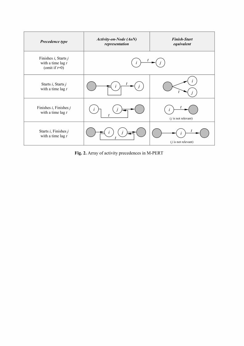
Consequently, the precedence relationships are necessarily represented by means of the 392

arrows connecting the nodes. Initially, it is well known that, given two activities i and j, there 393

can be four precedence relationships: Finishes i – Starts j (the most common by far), Starts i – 394

Starts j, Finishes i – Finishes j, and Starts i – Finishes j, all of them with or without time lags 395

between them. 396

Representation of the last three, despite being possible, significantly complicates the 397

network visualization and the critical path analysis when the number of activities is high 398

since some arrows depart the nodes from their back and/or reach the nodes at their front. 399

Fortunately, as recently found by Lu and Lam (2009), these three precedence types can be 400

reformulated as a Finish-Start relationship, as Figure 2 illustrates, and with which scheduling 401

students can be trained. Hence, from now on, M-PERT will make exclusive use of AoN 402

networks with Finish-Start (FS) precedence relationships, and should the user wish to 403

establish different types of precedence, he/she should refer to Figure 2, or, alternatively, to 404

Lu and Lam’s (2009) comprehensive treatment of non-finish-to-start relationships in project 405

networks, and transform them to FS relationships. 406

<Figure 2> 407

Essentially, M-PERT is a reduction technique in which project activities are merged by 408

groups of two or more, resulting in a new single merged activity, and this process is repeated 409

until there is just one activity left, which represents the total project duration. An idea of this 410

sequential merging procedure can be observed later in Figure 4 and the supplemental data. 411

The merging procedure was proposed by Cox (1995), and it is an intuitive and relatively 412

quick approach for reducing any (complex) network into a simple one. Of course, the 413

challenge is how to exactly merge different activities (which in the end correspond to 414

duration distributions). For that purpose and as justified earlier, it is assumed that the activity 415

durations follow a Normal distribution. Being aware that the specific probability distribution 416

18

was hardly important, the Normal assumption was also made by three out of the five methods 417

stated in Table 1, and this obeys the need of simplifying as much as possible the merging 418

operation of activities in series, which is the most frequent in any network. The merger 419

operations in the serial activities are represented in the first row of Figure 3. 420

<Figure 3> 421

Figure 3 is, in general, quite self-explanatory and basically represents the most common 422

operations (mergers) that can be found in any network – mostly serial activities (first row) 423

and maxima of multiple paths (bottom row) – along with other interesting operations that 424

GERT (Pritsker 1966) proposed (probabilistic paths, self-loops and activity minima) but was 425

not able to implement without ad hoc computational programmes. For illustrative purposes, 426

the case study shown later in Figure 4 will provide examples of these logic operations. 427

Particularly in construction projects, operations like probabilistic (alternative) paths might 428

seem quite straightforward for modelling uncertain courses of action that will mostly depend 429

on information that is still unknown, or at least inaccurate, at the conceptual stage. Examples 430

are the choice between different types of foundations depending on the ground conditions or 431

the soil-bearing capacity, or just the need to take special measures if the project uncovers 432

archeological remains. 433

Self-loops, on the other hand, are helpful for representing activities being repeated after 434

an unsuccessful outcome. These activities can correspond to isolated activities (e.g., a load 435

test, a calibration) or even groups of activities (e.g., a whole project drawing up process, a 436

series of defective structural elements, a non-compliant subnetwork within a water supply 437

system). It is up to the scheduler, however, to decide how many loops, or even how many 438

multiple nested loops, could be feasibly implemented before the construction manager or the 439

client stops the iterations. 440

19

Similarly, activity minima, despite certainly being much less frequent than activity 441

maxima, can also be useful at times to allow the project continuation after one (or some) of 442

the predecessors are finished. A distinctive quality of activity minima versus probabilistic 443

paths is that all the activities involved in the minima merger must be executed at some point 444

before the project finishes, whereas in probabilistic paths only one (or a subset of) path(s) 445

will be finally carried out. Examples of activity minima are the supply of any 446

electromechanical equipment among a series of any other equipment that needs to be 447

received in a worksite before the mechanical engineers can start working, or the clearance of 448

any stocking areas of a linear worksite before a new pipeline section can be supplied. 449

Overall, for every operation by rows in Figure 3, their representation (second column) is 450

shown; the input parameters (third column) necessary for defining the activities and 451

performing the merger into a single activity (which is generically named k) are provided; the 452

output parameters (fourth column) that define the new duration mean and variance of the 453

resulting merged activity k are provided; a representation of the result (fifth column) is 454

shown; and, finally, some observations (last column on the right) that clarify how to apply the 455

merger operations in particular (more complex) contexts. 456

It is worth highlighting that M-PERT requires that the activity duration means (μi) and 457

variances (σi) have been specified for each activity beforehand, a requirement that forces the 458

student or scheduler to elicit them or, if he/she wanted to start from the three-point estimates 459

(O, L and P), it would require a first stage of application of equations 1 and 2 (with the 460

correction proposed in equation 6) for each activity, like the original PERT. 461

Concerning the origin of the mathematical expressions stated for all the mergers (stated in 462

the Output parameters column), the serial activities merger just corresponds to the sum of 463

means and variances of several Normal distributions (as in equations 3 and 4), whereas the 464

expressions for the probabilistic alternative paths and the self-loops are easily derived from 465

20

the mathematical expressions of the mixture (Union) of n non-overlapping (Normal) 466

population samples (Xi=X1 … Xn), which are: 467

=i X

i XXk

i

ii

WW

(7) 468

( )( )2

222 <+=

i X

ji XXXX

i X

i XXk

i

jiji

i

ii

W

WW

WW

(8) 469

Where the WXi are the weights of each Normal population merged, that is, the proportion 470

by which that Normal distribution (representing a set of previously merged activities’ 471

duration) will be present in the resulting distribution after the next merger. For example, for 472

the probabilistic paths, the weights are the probabilities of each path occurring, that is, WX1=p 473

and WX2=1-p for two paths; or WXi=px for i=x=1,2,…n paths, with 11

==

n

xxW always. For the 474

self-loops, an activity i is merged with itself – activity i’s mean µX1=µi and standard deviation 475

σX1=σi when the activity happens just once with probability WX1=1-pi, and µX2=2µi and σX2= 2476

σi when it is repeated with probability WX2=pi. 477

Finally, the case of the maximum from two Normal distributions (the durations of two 478

activities) was coincidentally proposed by Clark (1961) but at that time it required intensive 479

use of tables and did not allow for correlation (ρ) between both activities. In particular, the 480

expression for the maximum was taken from Sculli and Shum (1991) and was also used by 481

Cox (1995), whereas the expression for the minimum was taken from Nadarajah and Kotz 482

(2008). Both expressions, despite looking long, are very easy to calculate. 483

The obvious problem with the maxima and minima from several activities is that the 484

formulae only allow for the merger of two of them at the same time. Then these expressions 485

can be applied recursively until there is just one activity left, a moment in which the activity 486

will be in series again and can keep being merged with its neighbor activities in series. This 487

recursive merging procedure is not new either, as it was successfully applied by Cox (1995), 488

21

Gong and Hugsted (1993) and Sculli and Shum (1991). However, it is also true that when 489

more than two activities are merged, there is a small error in the final mean and variance 490

calculation, which is also dependent (but to a minimum extent) on the exact merger order too. 491

Simulations performed that try to estimate the maximum error magnitude with M-PERT 492

identified how this error is maximized when the different paths’ duration mean is the same, 493

and variances are also identical between the parallel paths. However, even in that case, the 494

error obtained when merging “eight” activities under the same node (which is a higher 495

number than most of the real projects have under one converging node) causes an error of 496

6.7‰ in the mean and 7.3% in the standard deviation, which are considered, in general, good 497

approximations. 498

Therefore, M-PERT consists of merging activities until there is one activity left that 499

models the total project duration by means of μp and σp , which correspond to the project 500

duration mean and standard deviation, respectively. The order in which merger operations are 501

performed is relevant too. For example, if a self-loop comprised several activities, those inner 502

activities should first be merged, and then the self-loop resolved; or, if there are several 503

activities in series within a parallel path, those activities need to be merged before the path 504

can be merged with other paths. Overall, there must be an overriding use of common sense 505

when performing the mergers, and unless there is correlation among activities (a situation that 506

will be treated separately later), the merging procedure is quite straightforward. 507

There is just one last step left in the application of M-PERT. Obviously, the resulting 508

distribution modelling the total project duration is forced to be Normal in M-PERT, but, in 509

reality, this distribution might be more similar to an Extreme Value distribution when there is 510

a “high number of parallel paths converging all of them to the same node (activity)”. This is 511

not a secret, but it was not properly incorporated in a PERT model until Dodin and Sirvanci 512

22

(1990). He proposed using the Gumbel distribution (despite it being generically named the 513

Extreme Value distribution) for modelling the total project duration. 514

In M-PERT, however, we think the Normal distribution constitutes a reasonable 515

approximation. This is because most construction projects, despite usually including multiple 516

paths, they do not “all converge in the same single activity”, rather they have multiple paths 517

which converge at different activities. In other words, there is not a dominance of maxima 518

computation, but some maxima calculations mixed with a high number of activities in series 519

or activity maxima in series, both of which quickly degenerate (as shown in Figure 1) in 520

Normal distributions. Furthermore, students who are exposed to learning M-PERT are much 521

more familiar with the Normal distribution than with Extreme Value distributions. 522

523

Case study 524

A fictitious and simplified bridge project 525

M-PERT can be equally applied to simple and complex networks, the only difference 526

being the number of mergers that are required to be performed before the network is reduced 527

to a single activity representing the project duration. In this regard, Figure 4 presents the 528

application in a simple but representative bridge project construction with three piles (three 529

parallel paths), in which, purposefully, all possible kinds of merging operations have been 530

included. The activities ‘Start’ and ‘End’ are just dummy activities (null duration). 531

<Figure 4> 532

On the lower part of Figure 4, the sequential merging procedure has been exemplified. 533

Note, however, that the activities represent the standard deviation, not the variance, and this 534

is to be considered when applying all the expressions stated in Figure 3. Furthermore, the 535

type of merger operation has been stated in the five-step (solution) reduction procedure, 536

replacing the original activity descriptions and allowing the reader to understand where each 537

23

newly merged activity came from. All these indications however, are not necessary when we 538

try to expedite the manual calculation process. 539

Few explanations are needed at this stage, since the merger procedure just requires the 540

application of simple mathematical expressions already introduced mostly in Figure 3. It is 541

worth highlighting that, unlike the original PERT with fixed paths (in which what was 542

described in the network had to be necessarily carried out and excluded the possibility of 543

going backwards), the introduction of probabilistic paths, minima and self-loops allows for a 544

closer representation of construction projects. In this sense, M-PERT allows for some paths 545

happening while others do not, and that a group (or even the whole project if need be) is 546

repeated thanks to the inclusion of a self-loop. Overall, the modelling possibilities of M-547

PERT are significantly more powerful than the original PERT. 548

549

Networks with correlation between activities 550

Sometimes there are networks (project schedules) in which the merger procedure ends in 551

a knot that cannot be untangled. This is quite usual indeed when there are several parallel 552

paths that do not depart from the same node and/or do not converge in the same node 553

(Mehrotra et al. 1996). In those situations, the partially reduced network can end up in 554

(sub)networks similar to the ones shown in Figure 5, although maybe with more nodes. 555

<Figure 5> 556

For solving these subnetworks that usually represent a small portion of the whole 557

network, authors like Mehrotra et al. (1996) and Sculli and Shum (1991) proposed a 558

sequential recursive procedure that involves calculating all the variance and covariance 559

values between the ‘untangled’ paths. Implementing this procedure basically requires 560

identifying all the possible paths and then merging them, first, two of them, and then one by 561

24

one with the already merged group. However, the user needs to be aware that there is a 562

correlation (ρ≠0) between activities when applying the maxima (or minima) expressions from 563

Figure 3, that is, between paths that have some activities in common (as the covariance 564

between those two paths will not generally be zero). 565

As can be seen in Figure 5, identifying all the possible paths is not difficult unless the 566

network knot size involves a lot of activities and is very dense in precedence relationships 567

(number of arrows). The only tricky part is to calculate the correct value of ρ between the 568

paths. However, Sculli and Shum (1991) derived the generic expression for obtaining it, but 569

since that expression is somehow difficult to understand for the beginner, the ρ expressions 570

for up to four parallel paths (normally ordered from higher to lower mean duration µk and 571

sequentially named A, B, C and D) are given here: 572

BA

ABAB

COV= (9) 573

( ) ( )( )CAB

ABBCABACABC

ΦCOVΦCOV +=

1 (10) 574

( ) ( )( )[ ] ( ) ( )( )DABC

ABCCDABCABBDABADABCD

ΦCOVΦΦCOVΦCOV ++=

11 (11) 575

Where ρAB, ρABC, ρABCD representing, respectively, the correlation coefficients as paths A 576

with B, AB with C, and ABC with D are merged one by one with the previously merged 577

paths. COVXY simply corresponds to the sum of variances of the activities that paths X and Y 578

have in common, and σX and σY, the standard deviations of the paths X and Y respectively, 579

with X,Y=A, B, C, D. Examples of calculation of the variance and covariance values have 580

been provided in Figure 5 in the covariance matrices. 581

Finally, for the sake of clarity, the complete step-by-step procedure for implementing 582

expressions 9 to 11 in a project network with four paths with correlation has been described 583

25

in the supplemental data under Alternative 2 in the example project 0, along with other 584

multiple examples of M-PERT exercises. 585

586

Results 587

The five methods from which M-PERT has been built were tested in several benchmark 588

networks. There is no reason to believe that M-PERT, which makes use of their most 589

meritorious contributions, even including new features for better modelling real-life projects, 590

will have a lower accuracy. Anyhow, M-PERT has been applied to one network in this paper 591

and its accuracy comparison is presented in Figure 6. 592

<Figure 6> 593

It must be borne in mind, though, that Figure 6 shows a comparison of four statistical 594

distributions of which the distribution parameters are perfectly known, not a comparison of 595

datasets against another dataset or a known distribution, as is more usual in research analyses. 596

Hence, we will not be testing how ‘significant’ the difference between any two distributions 597

is, as it is already known that they are different distributions. Instead, a graphical approach is 598

adopted here for illustrating the location and dispersion deviations between the distributions. 599

Figure 6, in particular, shows four curves. The two continuous gray curves show the 600

exact solution of the project duration distribution (obtained through computer simulations) by 601

modelling the activity durations with Normal distributions and Uniform distributions 602

respectively. As stated before, the choice of one or other distribution hardly has any 603

relevance, an outcome proven again by observing how close both gray curves are. The 604

average (project duration) of these two simulated distributions is close to 147.5 days despite 605

they being lightly positively skewed and leptokurtic. 606

The dashed curve, on the other hand, represents the approximation offered by M-PERT 607

by using the Normal distribution modelling the project duration distribution, whose 608

26

parameters were obtained at the bottom of Figure 4. The bridge project, with three dominant 609

parallel paths, does not deviate much from the Normal approximation. It is also easy to 610

appreciate how the M-PERT project duration mean is close to 147 days (estimation error 611

below 1% when compared to the simulated curves, whereas the variance or dispersion error is 612

also below 10%). 613

Last of all, the continuous black curve representing the classical PERT approximation 614

significantly falls behind, with an average project duration of 133 days (error above 10%). 615

Again, this evidences how inaccurate the original PERT is when there are parallel paths and 616

the merge event bias is neglected. 617

Finally, for reassurance, results in other networks exemplifying step-by-step calculations, 618

along with the (simulated) actual project duration distribution, can be found as supplemental 619

data. 620

621

Discussion and conclusions 622

A new scheduling technique named M-PERT has been proposed. This technique takes 623

advantage of several methods that were proposed since PERT was devised for correcting 624

several shortcomings that the original technique had. In particular, in situations with multiple 625

parallel paths (the norm in construction projects), the original PERT resulted in a project 626

duration underestimation and a variance overestimation. 627

A systematic literature review has been developed in order to justify why M-PERT 628

concentrates on the really significant weaknesses of PERT and why, by neglecting other 629

accessorial aspects, the resulting tool is still accurate, but not complex. Indeed, the method 630

proposed is easy to implement and easy to learn due to its intuitive nature and simplifying 631

assumptions. This makes M-PERT an attractive tool for teaching scheduling basics to 632

construction and project management students, especially since its calculations can be 633

27

developed manually or by means of very simple spreadsheets. Finally, an application has 634

been included in which the new features offered by M-PERT, such as the minima of 635

activities, probabilistic (alternative) paths or activity or groups of activities self-loops 636

evidence a higher resemblance between scheduled networks and real construction projects. 637

However, there is still a long way to go. Indeed, despite this tool really departing from the 638

original PERT conception, it is still open to improvement. The cost dimension has not been 639

included in M-PERT, but it should follow a very similar approach. However, the inclusion of 640

resources in the analysis really represents a challenging route that should probably be 641

incorporated in the next versions of this scheduling technique. 642

643

Data availability 644

All data generated or analyzed during the study are included in the submitted article or 645

supplemental materials files. 646

647

References 648

Abbasi, G. Y., and Mukattash, A. M. (2001). “Crashing PERT networks using mathematical 649 programming.” International Journal of Project Management, 19(3), 181–188. 650

Ang, A. H.-S., Chaker, A. A., and Abdelnour, J. (1975). “Analysis of Activity Networks 651 under Uncertainty.” Journal of the Engineering Mechanics Division, 101(4), 373–387. 652

Anklesaria, K. P., and Drezner, Z. (1986). “A Multivariate Approach to Estimating the 653 Completion Time for PERT Networks.” Journal of the Operational Research Society, 654 37(8), 811–815. 655

Asmar, M. El, Hanna, A. S., and Whited, G. C. (2011). “New Approach to Developing 656 Conceptual Cost Estimates for Highway Projects.” Journal of Construction Engineering 657 and Management, American Society of Civil Engineers, 137(11), 942–949. 658

Azaron, A., Katagiri, H., Sakawa, M., Kato, K., and Memariani, A. (2006). “A multi-659 objective resource allocation problem in PERT networks.” European Journal of 660 Operational Research, 172(3), 838–854. 661

Azaron, A., and Tavakkoli-Moghaddam, R. (2007). “Multi-objective time–cost trade-off in 662 dynamic PERT networks using an interactive approach.” European Journal of 663 Operational Research, 180(3), 1186–1200. 664

Aziz, R. F. (2014). “RPERT: Repetitive-Projects Evaluation and Review Technique.” 665

28

Alexandria Engineering Journal, 53(1), 81–93. 666

Ballesteros-Pérez, P., Skitmore, M., Das, R., and del Campo-Hitschfeld, M. L. (2015). 667 “Quick Abnormal-Bid–Detection Method for Construction Contract Auctions.” Journal 668 of Construction Engineering and Management, 141(7), 4015010. 669

Banerjee, A., and Paul, A. (2008). “On path correlation and PERT bias.” European Journal 670 of Operational Research, 189(3), 1208–1216. 671

Baradaran, S., Fatemi Ghomi, S. M. T., Mobini, M., and Hashemin, S. S. (2010). “A hybrid 672 scatter search approach for resource-constrained project scheduling problem in PERT-673 type networks.” Advances in Engineering Software, 41(7–8), 966–975. 674

Baradaran, S., Fatemi Ghomi, S. M. T., Ranjbar, M., and Hashemin, S. S. (2012). “Multi-675 mode renewable resource-constrained allocation in PERT networks.” Applied Soft 676 Computing, 12(1), 82–90. 677

Bein, W. W., Kamburowski, J., and Stallmann, M. F. M. (1992). “Optimal Reduction of 678 Two-Terminal Directed Acyclic Graphs.” SIAM Journal on Computing, 21(6), 1112–679 1129. 680

Castro, J., Gómez, D., and Tejada, J. (2007). “A project game for PERT networks.” 681 Operations Research Letters, 35(6), 791–798. 682

Chen, S.-P. (2007). “Analysis of critical paths in a project network with fuzzy activity times.” 683 European Journal of Operational Research, 183(1), 442–459. 684

Cho, S. (2009). “A linear Bayesian stochastic approximation to update project duration 685 estimates.” European Journal of Operational Research, 196(2), 585–593. 686

Clark, C. E. (1961). “The Greatest of a Finite Set of Random Variables.” Operations 687 Research, INFORMS, 9(2), 145–162. 688

Clark, C. E. (1962). “Letter to the Editor—The PERT Model for the Distribution of an 689 Activity Time.” Operations Research, INFORMS, 10(3), 405–406. 690

Cox, M. (1995). “Simple normal approximation to the completion time distribution for a 691 PERT network.” International Journal of Project Management, 13(4), 265–270. 692

Creemers, S., Leus, R., and Lambrecht, M. (2010). “Scheduling Markovian PERT networks 693 to maximize the net present value.” Operations Research Letters, 38(1), 51–56. 694

Dodin, B., and Sirvanci, M. (1990). “Stochastic networks and the extreme value distribution.” 695 Computers & Operations Research, 17(4), 397–409. 696

Douglas, D. E. (1978). “PERT and simulation.” WSC ’78 Proceedings of the 10th conference 697 on Winter simulation, IEEE, 89–98. 698

Elmaghraby, S. E. (1989). “The estimation of some network parameters in the PERT model 699 of activity networks: review and critique.” Advances in Project Scheduling (eds. 700 Slowinski & Weglarz), Elsevier, 371–432. 701

Foldes, S., and Soumis, F. (1993). “PERT and crashing revisited: Mathematical 702 generalizations.” European Journal of Operational Research, 64(2), 286–294. 703

Fulkerson, D. R. (1962). “Expected Critical Path Lengths in PERT Networks.” Operations 704 Research, 10(6), 808–817. 705

Golenko-Ginzburg, D. (1989). “PERT assumptions revisited.” Omega, 17(4), 393–396. 706

29

Gong, D., and Hugsted, R. (1993). “Time-uncertainty analysis in project networks with a new 707 merge-event time-estimation technique.” International Journal of Project Management, 708 11(3), 165–173. 709

González, G. E. G., Hernández, G. O., and Roldán, F. (2014). “Effect of Network’s 710 Morphology and Merge Bias Correction Procedures on Project Duration Mean and 711 Variance.” Procedia - Social and Behavioral Sciences, 119, 2–11. 712

Grubbs, F. E. (1962). “Attempts to Validate Certain PERT Statistics or ‘Picking on PERT.’” 713 Operations Research, 10(6), 912–915. 714

Hahn, E. D. (2008). “Mixture densities for project management activity times: A robust 715 approach to PERT.” European Journal of Operational Research, 188(2), 450–459. 716

Hajdu, M. (2013). “Effects of the application of activity calendars on the distribution of 717 project duration in PERT networks.” Automation in Construction, Elsevier B.V., 35, 718 397–404. 719

Hajdu, M., and Bokor, O. (2014). “The Effects of Different Activity Distributions on Project 720 Duration in PERT Networks.” Procedia - Social and Behavioral Sciences, 119, 766–721 775. 722

Healy, T. L. (1961). “Activity Subdivision and PERT Probability Statements.” Operations 723 Research, INFORMS, 9(3), 341–348. 724

Herrerías-Velasco, J. M., Herrerías-Pleguezuelo, R., and Van Dorp, J. R. (2011). “Revisiting 725 the PERT mean and variance.” European Journal of Operational Research, 210(2), 726 448–451. 727

Johnson, D. (1997). “The Triangular Distribution as a Proxy for the Beta Distribution in Risk 728 Analysis.” Journal of the Royal Statistical Society: Series D (The Statistician), 46(3), 729 387–398. 730

Kamburowski, J. (1989). “PERT networks under incomplete probabilistic information.” 731 Advances in Project Scheduling (eds. Slowinski & Weglarz), Elsevier, 433–466. 732

Kamburowski, J. (1997). “New validations of PERT Times.” Omega, 25(3), 323–328. 733

Khamooshi, H., and Cioffi, D. F. (2013). “Uncertainty in Task Duration and Cost Estimates: 734 Fusion of Probabilistic Forecasts and Deterministic Scheduling.” Journal of 735 Construction Engineering and Management, American Society of Civil Engineers, 736 139(5), 488–497. 737

Kotiah, T. C. T., and Wallace, N. D. (1973). “Another Look at the PERT Assumptions.” 738 Management Science, INFORMS, 20(1), 44–49. 739

Kuklan, H., Erdem, E., Nasri, F., and Paknejad, M. J. (1993). “Project planning and control: 740 an enhanced PERT network.” International Journal of Project Management, 11(2), 87–741 92. 742

Lau, H.-S., and Somarajan, C. (1995). “A proposal on improved procedures for estimating 743 task-time distributions in PERT.” European Journal of Operational Research, 85(1), 744 39–52. 745

López Martín, M. M., García García, C. B., García Pérez, J., and Sánchez Granero, M. A. 746 (2012). “An alternative for robust estimation in Project Management.” European 747 Journal of Operational Research, 220(2), 443–451. 748

30

Lu, M. (2002). “Enhancing Project Evaluation and Review Technique Simulation through 749 Artificial Neural Network-based Input Modeling.” Journal of Construction Engineering 750 and Management, American Society of Civil Engineers, 128(5), 438–445. 751

Lu, M., and Lam, H.-C. (2009). “Transform Schemes Applied on Non-Finish-to-Start Logical 752 Relationships in Project Network Diagrams.” Journal of Construction Engineering and 753 Management, 135(9), 863–873. 754

Ludwig, A., Möhring, R. H., and Stork, F. (2001). “A Computational Study on Bounding the 755 Makespan.” Annals of Operations Research, 102, 49–64. 756

MacCrimmon, K. R., and Ryavec, C. A. (1964). “An Analytical Study of the PERT 757 Assumptions.” Operations Research, 12(1), 16-37. 758

Magott, J., and Skudlarski, K. (1993). “Estimating the mean completion time of PERT 759 networks with exponentially distributed durations of activities.” European Journal of 760 Operational Research, 71(1), 70–79. 761

Malcolm, D. G., Roseboom, J. H., Clark, C. E., and Fazar, W. (1959). “Application of a 762 Technique for Research and Development Program Evaluation.” Operations Research, 763 7(5), 646-669. 764

Mehrotra, K., Chai, J., and Pillutla, S. (1996). “A study of approximating the moments of the 765 job completion time in PERT networks.” Journal of Operations Management, 14(3), 766 277–289. 767

Mohan, S., Gopalakrishnan, M., Balasubramanian, H., and Chandrashekar, A. (2006). “A 768 lognormal approximation of activity duration in PERT using two time estimates.” 769 Journal of the Operational Research Society, 58(6), 827–831. 770

Mouhoub, N. E., Benhocine, A., and Belouadah, H. (2011). “A new method for constructing 771 a minimal PERT network.” Applied Mathematical Modelling, Elsevier Inc., 35(9), 772 4575–4588. 773

Mummolo, G. (1997). “Measuring uncertainty and criticality in network planning by PERT-774 path technique.” International Journal of Project Management, 15(6), 377–387. 775

Nadarajah, S., and Kotz, S. (2008). “Exact distribution of the max/min of two Gaussian 776 random variables.” IEEE Transactions on Very Large Scale Integration (VLSI) Systems, 777 16(2), 210–212. 778

Nelson, R. G., Azaron, A., and Aref, S. (2016). “The use of a GERT based method to model 779 concurrent product development processes.” European Journal of Operational 780 Research, 250(2), 566–578. 781

Pleguezuelo, R. H., Pérez, J. G., and Rambaud, S. C. (2003). “A note on the reasonableness 782 of PERT hypotheses.” Operations Research Letters, 31(1), 60–62. 783

PMI. (1996). A Guide to the Project Management Body of Knowledge. 1st edition. Project 784 Management Institute. Newton square, USA. 785

PMI. (2008). A Guide to the Project Management Body of Knowledge. 5th edition. (P. M. I. 786 N. square. USA, ed.), Project Management Institute. Newton square, USA. 787

Pontrandolfo, P. (2000). “Project duration in stochastic networks by the PERT-path 788 technique.” International Journal of Project Management, 18, 215–222. 789

Premachandra, I. M. (2001). “An approximate of the activity duration distribution in PERT.” 790

31

Computers and Operations Research, 28(5), 443–452. 791

Pritsker, A. A. B. (1966). GERT: Graphical Evaluation and Review Technique. RM-4973-792 NASA. National Aeronautics and Space Administration under Contract No. NASr-21. 793 Retrieved 2006-12-05. 794

Ringer, L. J. (1969). “Numerical Operators for Statistical Pert Critical Path Analysis.” 795 Management Science, 16(2), 136–143. 796

Sasieni, M. W. (1986). “Note—A Note on Pert Times.” Management Science, INFORMS, 797 32(12), 1652–1653. 798

Sculli, D., and Shum, Y. W. (1991). “An approximate solution to the pert problem.” 799 Computers & Mathematics with Applications, 21(8), 1–7. 800

Stauber, B. R., Douty, H. M., Fazar, W., Jordan, R. H., Weinfeld, W., and Manvel, A. D. 801 (1959). “Federal Statistical Activities.” The American Statistician, 13(2), 9–12. 802

Tatterson, J. (1974). “PERT, CPM and the export process.” Omega, 2(3), 421–426. 803

Tavares, L. V. (2002). “A review of the contribution of Operational Research to Project 804 Management.” European Journal of Operational Research, 136(1), 1–18. 805

Trietsch, D., and Baker, K. R. (2012). “PERT 21: Fitting PERT/CPM for use in the 21st 806 century.” International Journal of Project Management, APM and IPMA and Elsevier 807 Ltd, 30(4), 490–502. 808

Trietsch, D., Mazmanyan, L., Gevorgyan, L., and Baker, K. R. (2012). “Modeling activity 809 times by the Parkinson distribution with a lognormal core: Theory and validation.” 810 European Journal of Operational Research, Elsevier B.V., 216(2), 386–396. 811

Vanhoucke, M. (2012). Project Management with Dynamic Scheduling. Springer Berlin 812 Heidelberg, Berlin, Heidelberg. 813

Węglarz, J., Józefowska, J., Mika, M., and Waligóra, G. (2011). “Project scheduling with 814 finite or infinite number of activity processing modes – A survey.” European Journal of 815 Operational Research, 208(3), 177–205. 816

Wenying, L., and Xiaojun, L. (2011). “Progress Risk Assessment for Spliced Network of 817 Engineering Project Based on Improved PERT.” Systems Engineering Procedia, 1, 271–818 278. 819

Woolf, C. ., Cass, W., and McElroy, J. (1968). “The use of ‘Program Evaluation and Review 820 Technique’ (PERT) in the design and control of a medical research project.” Computers 821 and Biomedical Research, 2(2), 176–186. 822

Xiangxing, K., Xuan, Z., and Zhenting, H. (2010). “Markov skeleton process in PERT 823 networks.” Acta Mathematica Scientia, 30(5), 1440–1448. 824

Yaghoubi, S., Noori, S., Azaron, A., and Fynes, B. (2015). “Resource allocation in multi-825 class dynamic PERT networks with finite capacity.” European Journal of Operational 826 Research, Elsevier B.V., 247(3), 879–894. 827

828

1

▼Highlights Work ► Pritsker (1966)

Sculli and Shum (1991)

Gong & Hugsted (1993)

Cox (1995)

Mehrotra et al.

(1996)

Avoids having to calculate all the possible paths (critical and non-critical) (allows big networks)

ü ü ü

Allows for recursive application of activity maxima and/or minima (time-

saving simplification) ü ü ü

Normal distributions for modelling the activity durations

(only mean and variance matter) ü ü ü

Allows for correlation between different activities

(allows complex projects) ü ü ü ü

Use of simple expressions for solving the activity mergers

(calculation simplicity) ü ü

Allows for extra features (activity minima, self-loops or probabilistic paths, etc) (resemblance to reality)

ü

Number of benchmark networks in which the model was tested (Number

of validation tests) 4 2 3 2 10

Table 1. Key works on which PERT 2.0 has been based

Distribution of activity duration

Uniform (a=0, b=10)

Beta* (α=2.94,β=4.62,

a=0, b=15)

Distribution of activity duration

Uniform (a=0, b=10)

Beta* (α=2.94,β=4.62,

a=0, b=15)

*According to the original PERT, with Optimistic duration: 0, Most likely: 5, and Pessimistic: 15 time units.

Fig. 1. Comparison of two probability distributions alteration as more activities are added

0.000.020.040.060.080.100.12

0 2 4 6 8 10

Prob.

Duration0.000

0.002

0.004

0.006

0.008

0.010

0 5 10 15 20

Prob.

Duration0.000

0.002

0.004

0.006

0.008

0 5 10 15 20 25 30

Prob.

Duration

0.00

0.05

0.10

0.15

0 2 4 6 8 10 12 14 16

Prob.

Duration0.000

0.002

0.004

0.006

0.008

0.010

0 5 10 15 20 25 30

Prob.

Duration0.000

0.002

0.004

0.006

0.008

0 5 10 15 20 25 30 35

Prob.

Duration

0.000.020.040.060.080.100.12

0 2 4 6 8 10

Prob.

Duration0.00

0.05

0.10

0.15

0.20

0 2 4 6 8 10

Prob.

Duration0.00.10.10.20.20.30.3

0 2 4 6 8 10

Prob.

Duration

0.00

0.05

0.10

0.15

0 2 4 6 8 10 12 14 16

Prob.

Duration 0.000

0.005

0.010

0.015

0 2 4 6 8 10 12 14 16

Prob.

Duration0.000

0.005

0.010

0.015

0.020

0 2 4 6 8 10 12 14 16

Prob.

Duration

1

2

1

2

1

3

1

2

1 2

1

3

Precedence type Activity-on-Node (AoN) representation

Finish-Start equivalent

Finishes i, Starts j with a time lag t

(omit if t=0)

Starts i, Starts j with a time lag t

Finishes i, Finishes j with a time lag t

Starts i, Finishes j with a time lag t

Fig. 2. Array of activity precedences in M-PERT

j

i

t

j

i

t j

i

t

j

i t

i

t

( j is not relevant)

j

i t

i

t

( j is not relevant)

Operation AoN Representation Input par. Output parameters Result Observations

Serial activities

μi, σi² μj, σj²

… μn, σn²

¦

njix

xk,...,PP

¦

njix

xk,...,

22 VV

When there is a time lag t between any

two activities, then

μk= μi+μj+t and σk²=σi²+σj²

Probabilistic (alternative)

paths

μi, σi², p μj, σj², q=1-p

μk= p μi + (1-p) μj

σk²= p σi²+ (1-p) σj²+ p(1- p)(μi-μj)²

If there are more activities after any of the first activities from the paths, resolve

those mergers first, then merge into a single activity k

μx, σx², px

for x=1,2,3…n,

with ¦

n

xxp

11

¦

n

xxxk p

1PP

� � 2

1

222k

n

xxxxp

kPPVV �� ¦

Self-loops

μi, σi², pi μk= (1+pi) μi

σk²= (1+pi) σi²+ p(1- p)μi²

When the self-loop comprises more than one activity, resolve (merge) the activities within the loop first.

If there are nested (or multiple) self-loops, resolve inner self-loops first.

(maximum or minimum) Parallel

paths

Maximum (all activities are to finish before

continuing) or

Minimum (just one activity needs to finish

before continuing

μi, σi² μj, σj²

ρ (if i and j are correlated, otherwise ρ=0)

Maximum: � � � �� GITGPGPP �� ΦΦ jik 1 � � � � � � � �� 222222 1 kjijjiik ΦΦ PGITPPGPVGPVV ��

______________________________________

Minimum: � �� GITGPGPP �� ΦΦ jik 1 � � � �� 222222 1 kjijjiik ΦΦ PGITPPGPVGPVV ��

Where � � TPPG ji � ;

jiji VUVVVT 222 �� and φ(·) and Φ(·) are the Probability Density Function (PDF) and Cumulative Distribution Function (CDF) of the Standard Normal distribution (use Supplemental Figure 1 from the Supplemental

Online material for quick calculation)

When there are several activities on, at least, one path, resolve (merge) the

activities within that/those path/s first, then apply the maximum/minimum

merger.

When there are more than two alternative paths, keep recursively resolving

(merging) the paths by groups of two activities, until finishing with just one path (activity k will be then in series)

Fig. 3. Array of activity mergers in M-PERT

n

j

…

i

k

j

i

1-p

p

k

…

1 p…

p1

n

pn

i

pi

k

j

i

max/min

…

k

max/min

…

1+2 Serial merger

(35,5.10)

4

3+6+9 Serial merger

(90,12.25)

= (20,4)

5+8 Serial merger

(60,11.31)

7a+b

(11,12)min Minimum

(9.10,1.30)

10 =

(35,10)

13+14 Serial merger

(15,2.24)

16+17+18 Serial merger

(8,1) Prob. paths merger

(30,18.36)

MAX

0.50

15°

Self-loop (1.25,0.43)

Fig. 4. M-PERT application in a fictitious simplified bridge project

Start

1 Project

(30,5)

2 Site prep.

(5,1)

3 Excavations

(25,5)

4

5

Pile 2

6 Foundations

(25,5)

Excavations (20,4)

Excavations (30,8)

8 Foundations

(30,8)

7a Shallow found.

(20,4) 7b

11 Wind guards

(10,1)

12 Good weather

(10,2)

9 Concrete pile

(40,10)

10 Concrete pile

(35,10)

13 Crane install.

(10,2)

MIN 14 Pile erection

(5,1)

16 Traffic div.

(1,0)

17 Deck install.

(5,1)

1817 Load test

(2,0)

End

Deep foundations (60,10)

MAX 0.50

15

0.25

Pile load test (1,0)

Bridge Project (AoN network)

id Description

(μ,σ)

id: activity identifier μ: duration mean σ: duration std. dev.

Legend

(river)

Step-by-step merger procedure

1+2 =

(35,5.10)

4+7a+b+10+15°

3+6+9 =

(90,12.25)

Serial merger (86.25,21.29)

5+8+(11,12)min+13+14


(16+17+18)° Self-loop (12,4.18)

MAX

1+2 =

(35,5.10)

(3+6+9, 4+7a+b+10+15°)max

Maximum (98.04,13.73) (16+17+18)°

= (12,4.18) 5+8+(11,12)min+13+14

= (84.10,11.61)

1+2 =

(35,5.10)

[(3+6+9, 4+7a+b+10+15°)max , 5+8+(11,12)min+13+14]max

Maximum (100.29,11.84)

(16+17+18)° =

(12,4.18)

1+2+[(3+6+9, 4+7a+b+10+15°)max , 5+8+(11,12)min+13+14]max+(16+17+18)°


Step 1 (8 mergers)

Step 2 (3 mergers)

Step 4 (1 merger)

Step 5 (1 merger)

Step 3 (1 merger)

(final project)

Fig. 5. Two examples of AoN networks with correlation and the calculation of their covariance matrix

Start

1

2

4 5

3

7

6

8

9

End

Start 1

2

5

8

9

End

1

2

4

7

9

1

3

6

8

9

MAX

Path Activities μk A B C

A 1-2-4-7-9 μA=

μ1+μ2+μ4+μ7+μ9

σ2A=

σ21+ σ2

2+ σ24+ σ2

7+ σ29

COVAB=

σ21+ σ2

2+ σ29

COVAC=

σ21+ σ2

9

B 1-2-5-8-9 μB=

μ1+μ2+μ5+μ8+μ9 COVBA = COVAB

σ2B=

σ21+ σ2

2+ σ25+ σ2

8+ σ29

COVBC=

σ21+ σ2

8+σ29

C 1-3-6-8-9 μC=

μ1+μ3+μ6+μ8+μ9 COVCA = COVAC COVCB = COVBC

σ2C=

σ21+ σ2

3+ σ26+ σ2

8+ σ29

1

2

i (μi,σi)

i: activity identifier μi: duration mean

σi: duration std. dev.

Legend Start

3

4

End

1

2

Start

3

3

End 1

4

MAX

Path Activities μk A B C

A 1-3 μA = μ1+μ3 σ2A = σ2

1+ σ23 COVAB=σ2

1 COVAC=σ23

B 1-4 μB = μ1+μ4 COVBA = COVAB σ2B = σ2

1+ σ24 COVBC = 0

C 2-3 μC = μ2+μ3 COVCA = COVAC COVCB = COVBC σ2C = σ2

2+ σ23

Fig. 6. Comparison of project duration estimation accuracy between PERT and M-PERT for the simplified bridge project

0.00.10.20.30.40.50.60.70.80.91.0

100 110 120 130 140 150 160 170 180 190 200

Pro

babi

lity

Project Duration

Simulations (Normal) Simulations (Uniform) PERT M-PERT

- 1 -

Supplemental data

Contents

Detailed step-by-step calculations of the (Sub)network with correlation

Example Project 0 (page 2)

Alternative 1 (page 3)

Alternative 2 (general approach) (page 4)

Sample of 7 beginner-level exercises with increasing difficulty for learning M-PERT








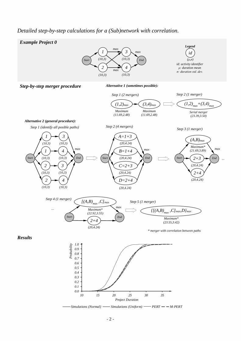
- 2 -

Detailed step-by-step calculations for a (Sub)network with correlation.

Results

0.0

0.1

0.2

0.3

0.4

0.5

0.6

0.7

0.8

0.9

1.0

10 15 20 25 30 35

Pro

ba

bil

ity

Project Duration

0.0

0.1

0.2

0.3

0.4

0.5

0.6

0.7

0.8

0.9

1.0

100 110 120 130 140 150 160 170 180 190 200

Pro

ba

bil

ity

Project Duration


(1,2)max (3,4)max

Maximum

(11.69,2.48) Maximum

(11.69,2.48)

(1,2)max

+(3,4)max


Start

1

(10,3)

3

End

max

2

(10,3)

4

(10,3)

(10,3)

1

4

(10,3) (10,3)

2

3

(10,3) (10,3)

Start

A=1+3

(20,4.24)

End

max

D=2+4

(20,4.24)

B=1+4

(20,4.24)

C=2+3

(20,4.24)

Start

(A,B)max

(20,4.24)

End

max

2+4

Maximum*

(21.69,3.89)

2+3

(20,4.24)

Start

[(A,B)max

,C]max

(20,4.24)

End

max

2+4

Maximum* (22.92,3.55)

{[(A,B)max

,C]max,D}max

Maximum* (23.55,3.42)

Alternative 1 (sometimes possible):

Step 1 (2 mergers) Step 2 (1 merger)

Alternative 2 (general procedure):

Step 1 (identify all posible paths) Step 2 (4 mergers)

…

…

Step 3 (1 merger)

Step 4 (1 merger) Step 5 (1 merger)

* merger with correlation between paths

Step-by-step merger procedure

Start

1

(10,3)

3

End

max

Example Project 0

id

(μ,σ)

id: activity identifier μ: duration mean

σ: duration std. dev.

Legend

2

(10,3)

4

(10,3)

(10,3)

max

max

- 3 -

Alternative 1

This alternative is possible due to the problem symmetry. If, for instance, the Finish-Start precedence

relationship between nodes 2 and 4 had not existed, this alternative would have not been possible, only

Alternative 2. However, when Alternative 1 is possible is always preferable since it is quicker and more

accurate (since normally it entails fewer recursive applications of the maximum merger formulae)

Step 1 (2 mergers)

■ Maximum merger between activities i=1 (with μi=10 and σi=3) and j=2 (with μj=10 and σj=3), then

k=(1,2)max. Values of Φ(·) and φ(·) can be calculated with the Supplemental Figure 1.

243.4183·3·0·2332 2222 jiji (there is no correlation between 1 and 2, i.e. ρ=0)

0243.41010 ji

693.11399.0·243.4

5.01·105.0·100243.401100101max)2,1(

ΦΦΦΦ jik

477.2135.6135.6

726.136399.0·86.845.01·1095.0·109693.110324.4101001103

01031

222

22222222

max)2,1(

2

k

kjijjiik

Φ

ΦΦΦ

■ Maximum merger between activities i=3 (with μi=10 and σi=3) and j=4 (with μj=10 and σj=3), then

k=(3,4)max.

In this case, it is obvious that since the means and variances of all the activities are the same, the result

coincides with the maximum merger for i=1 and j=2. Therefore, μk= μ(3,4)max =11.70 and σk=

σ(3,4)max=2.46

Step 2 (1 mergers)

■ Serial merger between activities i=(1,2)max. (with μi=11.693 and σi=2.477) and j=(3,4)max (with

μj=11.693 and σj=2.477), then k=(1,2)max+(3,4)max.

385.23693.11693.11,...,

max)4,3(max)2,1(

ji

njix

xk →Project Duration mean

503.3270.12270.12477.2477.2 2222

,...,

22

max)4,3(max)2,1(

2

kji

njix

xk →Project

Duration standard deviation

Now that μp=23.385 and σp=3.503 are known, the probabilities of any possible project duration (p) can

be calculated by using the Φ(z) curve in Supplemental Figure 1 with ppDz . Or the other

way around, that is, given a known probability Φ(z)=P (Y axis value), obtain the respective z value and

then pp zD .

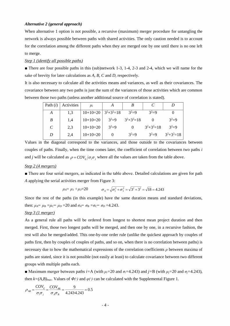
- 4 -

Alternative 2 (general approach)

When alternative 1 option is not possible, a recursive (maximum) merger procedure for untangling the

network is always possible between paths with shared activities. The only caution needed is to account

for the correlation among the different paths when they are merged one by one until there is no one left

to merge.

Step 1 (identify all possible paths)

■ There are four possible paths in this (sub)network 1-3, 1-4, 2-3 and 2-4, which we will name for the

sake of brevity for later calculations as A, B, C and D, respectively.

It is also necessary to calculate all the activities means and variances, as well as their covariances. The

covariance between any two paths is just the sum of the variances of those activities which are common

between those two paths (unless another additional source of correlation is stated).

Path (i) Activities μi A B C D

A 1,3 10+10=20 32+32=18 32=9 32=9 0

B 1,4 10+10=20 32=9 32+32=18 0 32=9

C 2,3 10+10=20 32=9 0 32+32=18 32=9

D 2,4 10+10=20 0 32=9 32=9 32+32=18

Values in the diagonal correspond to the variances, and those outside to the covariances between

couples of paths. Finally, when the time comes later, the coefficient of correlation between two paths i

and j will be calculated as jiijCOV where all the values are taken from the table above.

Step 2 (4 mergers)

■ There are four serial mergers, as indicated in the table above. Detailed calculations are given for path

A applying the serial activities merger from Figure 3:

μA= μ1 +μ3=20 243.41833 222

3

2

1 A

Since the rest of the paths (in this example) have the same duration means and standard deviations,

then: μA= μB =μC= μD =20 and σA= σB =σC= σD =4.243.

Step 3 (1 merger)

As a general rule all paths will be ordered from longest to shortest mean project duration and then

merged. First, those two longest paths will be merged, and then one by one, in a recursive fashion, the

rest will also be merged/added. This one-by-one order rule (unlike the quickest approach by couples of

paths first, then by couples of couples of paths, and so on, when there is no correlation between paths) is

necessary due to how the mathematical expressions of the correlation coefficients ρ between maxima of

paths are stated, since it is not possible (not easily at least) to calculate covariance between two different

groups with multiple paths each.

■ Maximum merger between paths i=A (with μi=20 and σi=4.243) and j=B (with μj=20 and σj=4.243),

then k=(A,B)max. Values of Φ(·) and φ(·) can be calculated with the Supplemental Figure 1.

5.0243.4·243.4

9

BA

AB

ji

ij

AB

COVCOV

- 5 -

243.418243.4·243.4·5.0·2243.4243.422 222222 BAABBAjijiAB

0243.42020 ABBAjiAB

AB

ABABABjABAjiBAk

ΦΦ

ΦΦΦΦ

693.21399.0·243.45.01·205.0·200324.40120020

11max),(

ABk

ABABABBAABBBABAA

kjijjiiBAk

ΦΦ

ΦΦ

ΦΦ

890.3132.15132.15586.470399.0·72.1695.01·4185.0·418

693.210324.420200120243.4020243.4

1

1

22222

22222

222222

max),(

2

Note that, for ease of notation, both results have been renamed as μAB and σAB.

Step 4 (1 merger)

■ Maximum merger between paths i=(A,B)max=AB (with μi=21.693 and σi=3.890) and j=C (with μj=20

and σj=4.243), then k=[(A,B)max ,C]=ABC. The expression for the coefficient of correlation calculation

is derived from Sculli & Shum (1991):

273.0

505.16

05.0·9

243.4·890.3

010091

ΦΦΦCOVΦCOV

CAB

ABBCABACABC

913.4120.24243.4·890.3·273.0·2243.4890.32 2222 CABABCCABABC

345.0913.420693.21 ABCCABABC

ABC

ABCABCABCCABCABABC ΦΦΦΦ

921.22376.0·913.4635.01·20635.0·693.21345.0912.4

345.0120345.0693.211

ABCk

ABCABCABCCABABCCCABCABABABC

ΦΦ

ΦΦ

548.3617.12

617.12372.525376.0·754.204635.01·418635.0·718.485921.22

345.0913.420693.21345.0120243.4345.0693.21890.3

1

2

2222

222222

Step 5 (1 merger)

■ Maximum merger between paths i=[(A,B)max,C]max=ABC (with μi=22.921 and σi=3.548) and j=D

(with μj=20 and σj=4.243), then k={[(A,B)max ,C]max,D}max=ABCD. The expression for the coefficient of

correlation calculation is derived from Sculli & Shum (1991):

408.0

054.15

635.01·9635.0·5.01·9

243.4·548.3

345.019345.001900

11

ΦΦΦΦ

ΦCOVΦΦCOVΦCOV

DABC

ABCCDABCABBDABADABCD

278.4305.18243.4·548.3·408.0·2243.4548.32 2222 DABCABCDDABCABCD

683.0278.420921.22 ABCDDABCABCD

- 6 -

nration meaProject Du

ΦΦΦΦ ABCDABCDABCDDABCDABCABCD

551.23316.0·278.4753.01·20753.0·921.22683.0278.4

683.0120683.0921.221

ationndard deviration staProject Du

ΦΦ

ΦΦ

k

ABCDABCDABCDDABCABCDDDABCDABCABCABCD

420.3695.11

695.11650.554316.0·616.183753.01·418753.0·960.537551.23

683.0278.420921.22683.0120243.4683.0921.22548.3

1

2

2222

222222

It is easy to see that, due to the recursive application of the maximum merger for the four paths, these

results (μp=23.551 and σp=3.420) do not exactly coincide with the previous from alternative 1

(μp=23.385 and σp=3.503), but they are very close. Again, the probabilities of any possible project

duration (p) can be calculated exactly as was explained for the Alternative 1.

0.00

0.05

0.10

0.15

0.20

0.25

0.30

0.35

0.40

0.45

0.50

0.55

0.60

0.65

0.70

0.75

0.80

0.85

0.90

0.95

1.00

0.00

0.05

0.10

0.15

0.20

0.25

0.30

0.35

0.40

0.45

0.50

0.55

0.60

0.65

0.70

0.75

0.80

0.85

0.90

0.95

1.00

-4.0 -3.5 -3.0 -2.5 -2.0 -1.5 -1.0 -0.5 0.0 0.5 1.0 1.5 2.0 2.5 3.0 3.5 4.0

Prob.

z φ(z) Φ(z)

Supplemental Figure 1. Abacus for calculating the probability density function φ(z) and the

cumulative distribution function Φ(z) of the Standard Normal distribution

- 7 -

Sample of 7 exercises (project schedules) of increasing difficulty for learning M-PERT

Note: for the calculations of the original PERT technique, self-loops are ignored (as they cannot be calculated with PERT)

and it has been assumed that the Critical Path goes through the path with higher probabilities of happening in presence of

probabilistic paths.

Results

0

0.1

0.2

0.3

0.4

0.5

0.6

0.7

0.8

0.9

1

80 90 100 110 120 130 140 150

Pro

babil

ity

Project Duration (t)

PERT PERT 2.0 Actual distrib.

0.0

0.1

0.2

0.3

0.4

0.5

0.6

0.7

0.8

0.9

1.0

100 110 120 130 140 150 160 170 180 190 200

Pro

ba

bil

ity

Project Duration


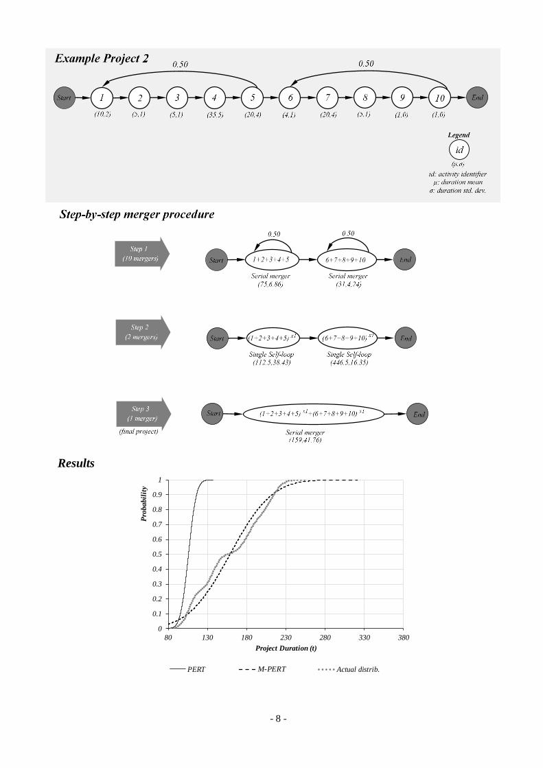
- 8 -

Results

0

0.1

0.2

0.3

0.4

0.5

0.6

0.7

0.8

0.9

1

80 130 180 230 280 330 380

Pro

ba

bil

ity



0.0

0.1

0.2

0.3

0.4

0.5

0.6

0.7

0.8

0.9

1.0

100 110 120 130 140 150 160 170 180 190 200

Pro

ba

bil

ity

Project Duration


- 9 -

Results

0

0.1

0.2

0.3

0.4

0.5

0.6

0.7

0.8

0.9

1

80 90 100 110 120 130 140 150

Pro

babil

ity



0.0

0.1

0.2

0.3

0.4

0.5

0.6

0.7

0.8

0.9

1.0

100 110 120 130 140 150 160 170 180 190 200

Pro

ba

bil

ity

Project Duration


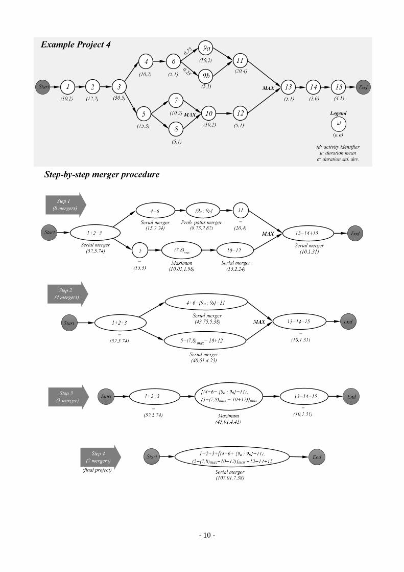
- 10 -

- 11 -

Results

0

0.1

0.2

0.3

0.4

0.5

0.6

0.7

0.8

0.9

1

80 90 100 110 120 130 140 150

Pro

bab

ilit

y



0.0

0.1

0.2

0.3

0.4

0.5

0.6

0.7

0.8

0.9

1.0

100 110 120 130 140 150 160 170 180 190 200

Pro

ba

bil

ity

Project Duration


- 12 -

- 13 -

Results

0

0.1

0.2

0.3

0.4

0.5

0.6

0.7

0.8

0.9

1

110 120 130 140 150 160 170 180 190

Pro

bab

ilit

y



0.0

0.1

0.2

0.3

0.4

0.5

0.6

0.7

0.8

0.9

1.0

100 110 120 130 140 150 160 170 180 190 200

Pro

ba

bil

ity

Project Duration


- 14 -

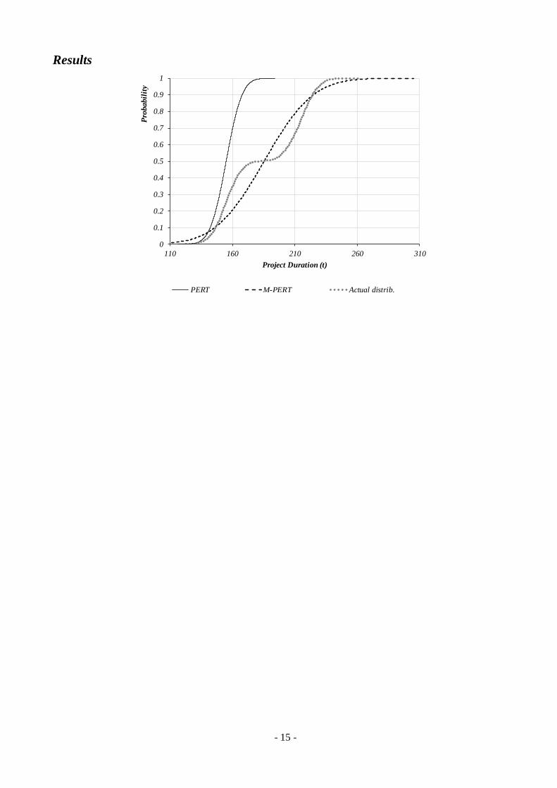
- 15 -

Results

0

0.1

0.2

0.3

0.4

0.5

0.6

0.7

0.8

0.9

1

110 160 210 260 310

Pro

ba

bil

ity



0.0

0.1

0.2

0.3

0.4

0.5

0.6

0.7

0.8

0.9

1.0

100 110 120 130 140 150 160 170 180 190 200

Pro

ba

bil

ity

Project Duration


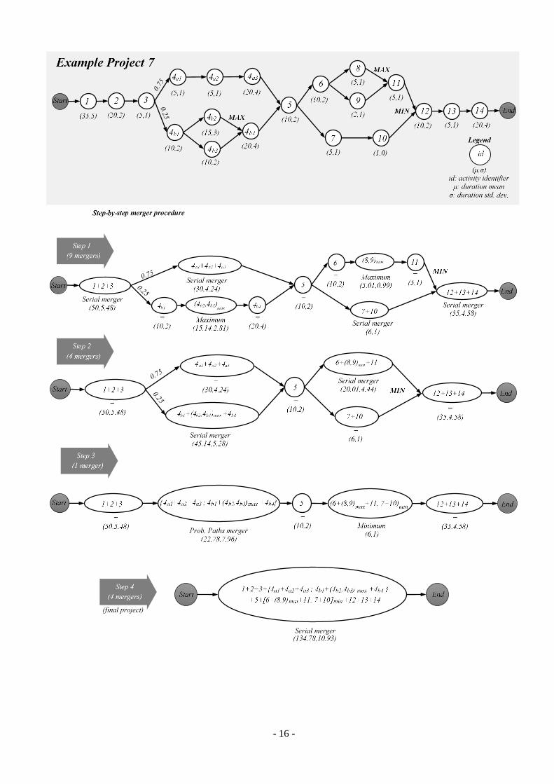
- 16 -

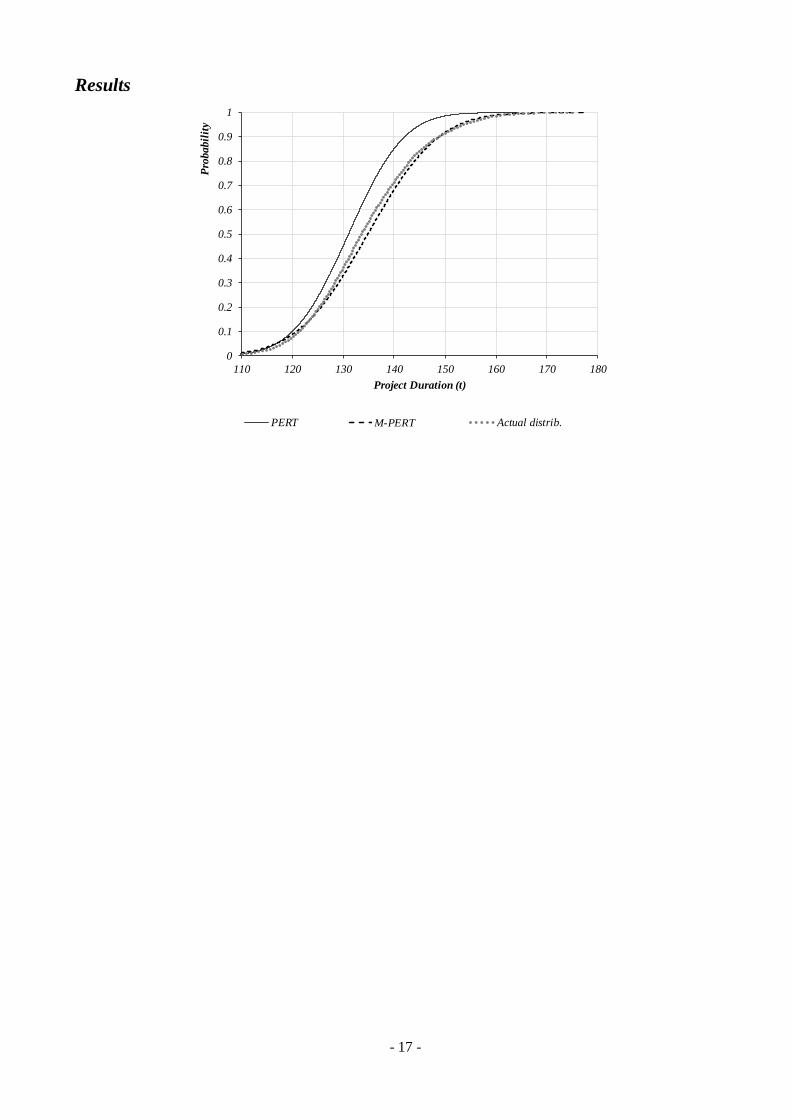
- 17 -

Results

0

0.1

0.2

0.3

0.4

0.5

0.6

0.7

0.8

0.9

1

110 120 130 140 150 160 170 180

Pro

babil

ity



0.0

0.1

0.2

0.3

0.4

0.5

0.6

0.7

0.8

0.9

1.0

100 110 120 130 140 150 160 170 180 190 200

Pro

ba

bil

ity

Project Duration


M-PERT: manual project-duration estimation technique for ...

Documents

Transcript of M-PERT: manual project-duration estimation technique for ...