M odel Selection using Inform ation T heory and …stine/research/smr.pdfM odel Selection using...

Model Selection using

Information Theory and the MDL Principle ∗

Robert A. Stine

Department of Statistics

The Wharton School of the University of Pennsylvania

Philadelphia PA 19104-6340

www-stat.wharton.upenn.edu/∼stine

February 6, 2003

Abstract

Information theory offers a coherent, intuitive view of model selection. This perspective

arises from thinking of a statistical model as a code, an algorithm for compressing data into a

sequence of bits. The description length is the length of this code for the data plus the length

of a description of the model itself. The length of the code for the data measures the fit of

the model to the data, whereas the length of the code for the model measures its complexity.

The minimum description length (MDL) principle picks the model with smallest description

length, balancing fit versus complexity. The conversion of a model into a code is flexible; one

can represent a regression model, for example, with codes that reproduce the AIC and BIC

as well as motivate other model selection criteria. Going further, information theory allows

one to choose from among various types of non-nested models, such as tree-based models and

regressions identified from different sets of predictors. A running example that compares several

models for the well-known Boston housing data illustrates the ideas.

∗I wish to thank Dean Foster and John Fox for many helpful suggestions.

1

Model selection using MDL (February 6, 2003) 2

1 Introduction

What’s the best model? Certainly, the beauty of a model lies in the eyes of the beholder. Perhaps

it’s the “most natural” model, one that embodies our notions of cause and effect, with its form

pre-ordained by our theory. Perhaps instead it’s the “simplest” model, one that is easy to describe

with few features determined from the data at hand. Alternatively, perhaps it’s just the “most

predictive” model, a model that predicts new observations more accurately than any other — a

black box that churns out predictions with no obligation for interpretation.

More likely, the best model blends these attributes — theory, parsimony, and fit. If so, how

should we balance these competing aims? How should we weigh the contribution of a priori theory

versus the fit obtained by an automated search through a large database? Indeed, some criteria offer

no reward for a strong theory. Naive use of the AIC and BIC, for example, implies that all regression

models with the same R2 and the same number of predictors are equivalent. Both measure the

quality of a model from only its fit to the data and the count of its estimated parameters. The

path that led to a model is irrelevant. To these, it does not matter whether we chose the predictors

a priori or discovered them using stepwise regression; theory and explanation can come before or

after estimation. It is little wonder that many view variable selection as mechanical optimization

devoid of substantive content. The criteria described here do reward the investigator with a model

chosen by theory, whether the theory indicate specific features of the model or opinions of what is

expected.

And what of Occam’s razor? Surely, if we have two regressions with the same R2, one with two

predictors and one with 20, common sense leads us to pick the model with just two predictors. But

the catalog of models offered by modern statistics software is much richer than regressions with

differing numbers of slopes. How, for example, can we compare a linear regression to a regression

tree, especially when both obtain comparable fits to the data? We can’t just count “parameters.”

The estimated parameters of these two types of models — estimated slopes in regression versus

group averages and optimal cut-points in trees — are too different.

In what follows, I answer these questions by adopting an information theoretic view of model

selection. Before delving into information theory, however, the next section describes three models

for the well-known Boston housing data. These models illustrate key points throughout this paper.


2 Three Models for Housing Prices

This section describes three models for the median housing price reported in the Boston housing

dataset which was created by Harrison and Rubinfeld (1978) to investigate the effects of pollution

on housing values. This dataset has 14 characteristics of the 506 census tracts with housing units in

the Boston SMSA in 1970. Table 1 lists the variables. The response for all three illustrative models

is the median value of owner-occupied homes. Two of the models are standard OLS regressions.

The third model is a regression tree. This dataset is on-line from Statlib at http://lib.stat.cmu.edu

or with the software package R at http://cran.r-project.org/. I used the data packaged with

R. Belsley, Kuh and Welsch (1980) popularized the use of this data in their study of regression

diagnostics. Others (e.g. Breiman and Friedman, 1985) have used it to illustrate data mining. It

has also been observed to contain censoring; the median value of homes is probably right-censored

at $50,000. I will not explore these issues further.

I fit these models to a subset of 50 tracts selected randomly from the full collection.1 The reason

for restricting the estimation to a subset is to weaken the effects of the predictors and thereby make

the problem of model selection more difficult. When fit to the full dataset, an OLS regression of

MEDV on the 13 remaining variables has an R2 of 74% with 11 predictors having absolute t-ratios

larger than 3. When fit to the subset, the effects become subtle; only three predictors have a t-ratio

larger than 3 in magnitude. Variable selection is more challenging when the effects are subtle;

virtually any method works in the presence of a strong, obvious signal.

The two illustrative regression models are the same, but I want to make a distinction in how they

were found. Suppose that my research concerns determinants of the value of housing. In particular,

I have a theory that proposes that young families with several children drive up demand for larger

houses, and that this group likes to have their big homes near good schools in safe communities.

The model shown in Table 2 embodies these ideas; the interaction between the number of rooms

and the pupil-teacher ratio RM*PTRATIO captures the notion that big houses lose value if they

are near crowded schools. One can imagine that I could have proposed the form of this model (i.e.,

picked the predictors) prior to looking at the data; its form originated in my theory rather than1I used the sample function from R to pick these, avoiding documented outliers. To reduce the effects of outliers,

I set aside 6 tracts (rows 366 and 369 – 373) from the full data set prior to sampling. The 50 sampled tracts are rows

18, 22, 25, 37, 43, 44, 46, 51, 58, 62, 69, 71, 74, 78, 90, 93, 100, 112, 126, 131, 135, 152, ,161, 170, 181, 190, 200,

203, 204, 212, 213, 221, 222, 235, 236, 268, 316 317, 321, 322, 391, 394, 397, 398, 417, 445, 462, 489, 495, 503 in the

Boston data distributed with R.


Table 1: The Boston housing dataset contains 14 variables that describe the 506 census tracts in

the Boston SMSA in 1970, excluding tracts with no housing units. (Harrison and Rubinfeld, 1978;

Belsley et al., 1980). Available on-line from Statlib (http://lib.stat.cmu.edu) or as part of the R

software package (http://cran.r-project.org).

MEDV median value of owner-occupied homes in $1000’s (response)

AGE proportion of owner-occupied units built prior to 1940

BLACK 1000(B − 0.63)2 where B is the proportion of blacks by town

CHAS Charles River dummy variable (1 bounds river; 0 otherwise)

CRIM per capita crime rate by town

DIS weighted distances to five Boston employment centres

INDUS proportion of non-retail business acres per town

LSTAT percentage lower status of the population

NOX nitric oxides concentration (parts per 10 million)

PTRATIO pupil-teacher ratio by town

RAD index of accessibility to radial highways

RM average number of rooms per dwelling

TAX full-value property-tax rate per $10,000

ZN proportion of residential land zoned for lots over 25,000 sq.ft.


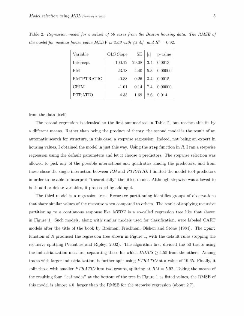
Table 2: Regression model for a subset of 50 cases from the Boston housing data. The RMSE of

the model for median house value MEDV is 2.69 with 45 d.f. and R2 = 0.92.

Variable OLS Slope SE |t| p-value

Intercept -100.12 29.08 3.4 0.0013

RM 23.18 4.40 5.3 0.00000

RM*PTRATIO -0.88 0.26 3.4 0.0015

CRIM -1.01 0.14 7.4 0.00000

PTRATIO 4.33 1.69 2.6 0.014

from the data itself.

The second regression is identical to the first summarized in Table 2, but reaches this fit by

a different means. Rather than being the product of theory, the second model is the result of an

automatic search for structure, in this case, a stepwise regression. Indeed, not being an expert in

housing values, I obtained the model in just this way. Using the step function in R, I ran a stepwise

regression using the default parameters and let it choose 4 predictors. The stepwise selection was

allowed to pick any of the possible interactions and quadratics among the predictors, and from

these chose the single interaction between RM and PTRATIO. I limited the model to 4 predictors

in order to be able to interpret “theoretically” the fitted model. Although stepwise was allowed to

both add or delete variables, it proceeded by adding 4.

The third model is a regression tree. Recursive partitioning identifies groups of observations

that share similar values of the response when compared to others. The result of applying recursive

partitioning to a continuous response like MEDV is a so-called regression tree like that shown

in Figure 1. Such models, along with similar models used for classification, were labeled CART

models after the title of the book by Breiman, Friedman, Olshen and Stone (1984). The rpart

function of R produced the regression tree shown in Figure 1, with the default rules stopping the

recursive splitting (Venables and Ripley, 2002). The algorithm first divided the 50 tracts using

the industrialization measure, separating those for which INDUS ≥ 4.55 from the others. Among

tracts with larger industrialization, it further split using PTRATIO at a value of 19.65. Finally, it

split those with smaller PTRATIO into two groups, splitting at RM = 5.92. Taking the means of

the resulting four “leaf nodes” at the bottom of the tree in Figure 1 as fitted values, the RMSE of

this model is almost 4.0, larger than the RMSE for the stepwise regression (about 2.7).


Figure 1: Regression tree for the median house price, estimated using the rpart function of R. The

collective standard deviation of the residuals about the averages of the 4 leaf nodes is 3.96.

|indus>=4.55

ptratio>=19.65

rm< 5.9215.01 19 23.74

38.21

Which of these three models is the best? Methods that select a model while ignoring how

it came into being cannot distinguish the two regressions. Methods that just count parameters

run into problems when comparing either regression to the tree. How many parameters are in

the regression tree in Figure 1? The fit at each leaf node is an average, but how should we treat

the splitting points that define the groups? Can we treat them like other parameters (slopes and

averages), or should we handle them differently? Research suggests that we need to assess such

split points differently. For example, Hinkley’s early study of inference for the break point in a

segmented model (Hinkley, 1970) suggests that tests for such parameters require more than one

degree of freedom.

The information theoretic view of model selection allows one to compare disparate models as

well as account for the origin of the models. The process leading to the model is, in essence, part of

the model itself, allowing MDL to reward a theoretical model for its a priori choice of predictors.

The information theoretic view is also flexible. One can compare different types of models, such as

the illustrative comparison of a regression equation to a regression tree.

3 A Brief Look at Coding

Good statistical models “fit well.” Although the notion of fit varies from one model to another,

likelihoods offer a consistent measure. By associating each model with a probability distribution,

we can declare the best fitting model as the one that assigns the largest likelihood to the observed


data. If the model has parameters, we set their values at the maximum likelihood estimates.

Coding offers an analogous sense of fit. A good code is an algorithm that offers high rates of

data compression while preserving all of the information in the data. The best code compresses data

into the shortest sequence of bits. If we think of our response as occupying a file on a computer,

then the best code for this response is the algorithm that compresses this file down to the smallest

size — while retaining information that allows us to recover the original data. The trick in seeing

how information theory addresses model selection is to grasp how we can associate a statistical

model with a scheme for coding the response.

Suppose that I want to compress a data file, say prior to sending it as an attachment to an

e-mail message. The heuristic of “sending a message to a receiver” is valuable in thinking about

coding data; it is essential to identify what the receiver already knows about the data and what

I have to tell her. If I can find a way to reduce the number of bits used to represent the most

common patterns in the data, then I can reduce the overall size of the message. Obviously, I have

to be able to do this unambiguously so as not to confuse the recipient of my e-mail; there must be

only one way for her to decode the attachment. Such representations are said to be lossless since

one can recover the exact source file, not just be close. Alternative “lossy” codes are frequently

used to send sounds and images over the Internet. These offer higher rates of compression but do

not allow one to recover the exact source image.

For the example in this section, the data to be compressed is a sequence of n characters drawn

from the abbreviated 4-character alphabet a, b, c, and d. Since coding is done in the digital

domain, I need to represent each character as a sequence of bits, 0s and 1s. The standard ASCII

code for characters uses 8 or 9 bits per letter – quite a bit more than we need here since we have

only 4 possibilities – but a simplified version works quite well. This fixed-length code (Code F)

appears in the second column of Table 3. Code F uses two bits for each of the four possible values.

For example, with n = 5, the attached sequence of 10 bits 0100000011 would be decoded by the

recipient as

0100001100 = 01 00 00 11 00 decode−→ b a a d a

where I use spaces to make the encoded data easier for us to read, but are not part of the code.

With Code F, it takes 2n bits to send n of these letters, and the attached data is easy to recover.

More knowledge of the data allows higher compression with no loss in content. More knowledge

in coding comes in the form of a probability distribution for the data. For example, suppose that


Table 3: Sample codes for compressing a random variable that takes on four possible values a, b, c,

and d with distribution p(y). Code F uses a fixed number of bits to represent each value, whereas

Code V varies the number of bits as given by − log2 p(y).

Symbol y Code F Code V p(y)

a 00 0 1/2 = 1/21

b 01 10 1/4 = 1/22

c 10 110 1/8 = 1/23

d 11 111 1/8 = 1/23

the data are a sample Y1, Y2, . . . , Yn of grades that have the distribution

p(y) =

1/2 if y = a ,

1/4 if y = b ,

1/8 if y = c ,

1/8 if y = d .

(1)

(Evidently, grade inflation is prevalent.) Code V in the third column of Table 3 conforms to these

probabilities. Code V uses a varying number of bits to represent the 4 symbols, with the number

of bits set to the negative of the base 2 log of the probability of each symbol. Thus, characters that

occur with high probability get short codes. For example, Code V uses only 1 bit (1 = − log2 1/2)

to represent the most likely symbol a, but uses three bits for the least likely symbols c and d.

Because of the varying length of the codes assigned by Code V, it may not be clear how to decode

the compressed data. To see how this works, let’s return to the previous example that encodes b, a,

a, d, and a. First, we’ll encode the data, then see how the receiver decodes it. Encoding is simply

a matter of concatenating the bits given in the third column of Table 3:

b a a d aencode−→ 10 0 0 111 0

Notice that the encoded message is shorter than the message obtained with Code F, requiring 8

bits rather than 10. The receiver of the message reverses this process. Basically, she parses the

sequence of bits one at a time until she matches one of the codes in the third column of Table 3.

The first character is a 1, which does not match any of the codes. The first two characters form

the sequence 10 which is the code for b. The next character is a 0, which matches the code for a.


Continuing in this fashion, she can recover the original sequence. Keep in mind, however, that the

receiver has to know Code V for this scheme to work.

Although Code V obtains higher compression for the sequence baada, it should also be apparent

that Code F compresses some other sequences better. For example, to encode dccab requires 10 bits

with Code F but consumes 12 bits for Code V. Code V is two bits better for one data series, but two

bits worse for another. Why bother with Code V? The answer lies in the underlying probabilities.

If the characters to be compressed are indeed a random sample with the distribution p(y) given in

(1), then the probability of the sequence for which Code V compresses better is

P(baada) = p(b) p(a) p(a) p(d) p(a)

= 14

12

12

18

12

= 122

12

12

123

12

= 1/28 .

The probability of the sequence for which Code V does worse is 16 times smaller:

P(dccab) = p(d) p(c) p(c) p(a) p(b)

= 123

123

123

12

122

= 1/212 .

Code V works well for sequences that are more likely according to the associated distribution p(y).

Higher probability means a shorter code. Code V represents baada using 8 bits, which is the

negative of the log (base 2) of the likelihood of this sequence under the model p(y),

Length of Code V for baada = !(baada)

= − log2 P (baada) = 8 .

Similarly, !(dccab) = − log2 P (dccab) = 12.

The Kraft inequality from information theory strengthens the connection between the length

of a code for a sequence of symbols and the probability of those symbols. The Kraft inequality

implies that however we decide to encode the characters in our message, we cannot have too many

short codes because (Section 5.2, Cover and Thomas, 1991)∑y

2−!(y) ≤ 1 , (2)

where the sum runs over all possible values for y and !(y) denotes the number of bits required to

encode y. A code is said to be “Kraft-tight” if it attains this upper bound; both codes in Table 3


are Kraft-tight. We can thus interpret 2−!(y) as a probability. That is, the Kraft inequality allows

us to define a probability from the lengths of a code. If a code is not Kraft-tight, it essentially has

reserved symbols for characters that cannot occur. Such codes can be improved by removing the

unnecessary terms. For example, using the 8-bit ASCII code for our 4 character problem would

not produce a Kraft-tight code.

Codes derived from a probability distribution obtain the best compression of samples from this

distribution. The entropy of a random variable determines the minimum expected code length.

The entropy of a discrete random variable Y ∼ p(y) is

H(Y ) = E log2 1/p(Y ) =∑y∈Y

p(y) log21

p(y). (3)

It can be shown that if !(y) is the length of any lossless code for the random variable Y , then

(Sections 5.3-5.4, Cover and Thomas, 1991)

E !(Y ) ≥ H(Y ) .

Thus the fixed-length Code F is optimal if the 4 values a, b, c and d are equally likely whereas

Code V is optimal if the probabilities for these symbols are 1/2, 1/4, 1/8, and 1/8, respectively.

What happens if one uses a code that does not conform to the underlying probabilities? The code

is longer, on average, than it needs to be.

For the illustrations, both probabilities have the convenient form p(y) = 2−j with j an integer

so that the code lengths are readily apparent and integers. In other cases, the method known

as arithmetic coding allows one to compress data within one bit of the entropy bound even when

the probabilities lack this convenient form. Given that one knows the true generating frequencies,

arithmetic coding allows one to compress Y1, . . . , Yn into a code whose expected length is bounded

by 1 + n H(Yi) (Langdon, 1984). As we continue, I will also ignore the need for an actual code to

have an integer length, using what is often called the idealized length (Barron, Rissanen and Yu,

1998).

To recap, the best code for a random variable Y ∼ p has idealized length

!(y) = − log2 p(y) , (4)

and the length of this code for representing a sample of n independent responses Y1, Y2, . . . , Yn ∼ p

is the negative log-likelihood,

!(y1, . . . , yn) = − log2 L(y1, . . . , yn)


= − log2 p(y1) p(y2) · · · p(yn) . (5)

The expected length of any other code for Y exceeds the resulting entropy bound (3). Analogous

properties hold for continuous random variables like the Gaussian or Cauchy as well. Even though

the likelihood L(y1, . . . , yn) for a continuous random variable no longer gives probabilities, the code

length retains the convenient form seen in (4). To get a sense for how coding applies to continuous

random variables, think of encoding a discrete approximation that rounds the continuous random

variable to a certain precision. Cover and Thomas (1991) (Section 9.3) shows that the length of the

code for the rounded values is the log-likelihood of the continuous data plus a constant that grows

as one keeps more digits. One can handle dependent sequences by factoring the log-likelihood as

!(y1, . . . , yn) = − log2 (p(y1) p(y2 | y1) p(y3 | y1, y2) · · · p(yn | y1, . . . , yn)) .

Thus, we can associate a model with a code by finding a code matched to the likelihood implied

by the model. The best code and the best model share a common heritage – both maximize the

likelihood for the observed data. But this presents a problem for model selection. If coding just

maximizes the likelihood, how does it avoid overfitting? The answer requires that we take a broader

look at our original task.

4 The Minimum Description Length Principle

Just because we can compress data optimally by maximizing its likelihood does not mean that

the recipient of our message can recover the original data. For this task, she needs to know how

we encoded the data — she must know our model. The codes described here convey the model

to her in a straightforward fashion. They include the parameter estimates as part of the message

to the receiver, prefixing the compressed data. Hence, such messages are called two-part codes.

The inclusion of the model as part of our message has a dramatic effect. A regression model with

10 estimated slopes might fit well and offer high compression of the data, but it also requires us

to convey 10 estimated parameters to the receiver. A simpler regression with just two estimated

slopes need only add 2. Unless the gain in compression (i.e., the increase in the likelihood) is

enough to compensate for the 8 additional estimates, the simpler model may in fact produce a

shorter message.

Rissanen’s minimum description length (MDL) principle (Rissanen, 1978) formalizes this idea.

The description length of a fitted model is the sum of two parts.2 The first part of the description2Stochastic complexity, introduced in Rissanen (1986), enhances the MDL principle by removing redundancies


length represents the complexity of the model. This part encodes the parameters of the model itself;

it grows as the model becomes more complex. The second part of the description length represents

the fit of the model to the data; as the model fits better, this term shrinks. A precise definition

requires a bit of notation. Let Mθ denote a parametric model indexed by a parameter vector θ,

and let L(· | Mθ) denote the likelihood implied by this model. Also, let Y denote n observations

y1, y2, . . . , yn of the response. Since we obtain the shortest code for the data by maximizing the

likelihood, the MLE for θ, say θ(Y ), identifies the optimal model. The resulting description length

of such a model is

D(Y ;Mθ(Y )) = !(Mθ(Y ))− log2 L(Y | Mθ(Y )) . (6)

The MDL principle picks the model with the minimum description length. To compute the de-

scription length, though, we need to determine how many bits are required to encode the model

Mθ(Y ) itself.

At this point, the flexibility and Bayesian flavor of coding emerge. Recall that every code

embodies a probability distribution. Thus, any code for the model Mθ(Y ) also implies a probability

distribution, one for the model itself. In the case of parametric models such as regression, the code

must give the parameters that identify the specific model. The length of this code depends on

which values we expect for θ(Y ). Choose poorly and one faces a rather large penalty for adding a

parameter to the model.

Before describing how to encode the whole model, we need to consider first how to encode a

single parameter. Since θ(Y ) is unlikely to be an integer, it is not obvious how to represent θ(Y )

with a discrete code. Fortunately, Rissanen (e.g. Rissanen, 1989, Section 3.1) shows that we can, in

fact, round the MLE with little loss in data compression. The idea is to round θ(Y ) to the nearest

coordinate of the form θ0 + z SE(θ(Y )) for integer z and define the estimator

θ(Y ) = θ0 + SE(θ(Y ))⟨

θ(Y )− θ0

SE(θ(Y ))

⟩= θ0 + SE(θ(Y )) 〈 zθ(Y ) 〉 , (7)

where 〈x 〉 denotes the integer closest to x. The rounded estimator lies within half of a standard

error of the MLE, falling on the grid centered at a default value θ0 (typically zero) plus a multiple

〈 zθ(Y ) 〉 of the standard error. Rounding a vector of estimates is considerably more complex but

follows the this paradigm: approximate the MLE using a grid resolved to the nearest standard

error (Rissanen, 1983).

inherent in a two-part code. While theoretically appealing, the results for model selection are essentially identical.

The accompanying idea, known as parametric complexity, introduces other complications (Foster and Stine, 2003).


This rounding has negligible effect on the length of the second part of the code. If we encode

the data using θ rather than the MLE, the length of the compressed data grows by less than a bit.

(This result is perhaps one of the strongest arguments for showing rounded estimates in presenting

statistical output. All of those superfluous digits offer no help in coding the data.) So, in practice,

the description length is computed not as in (6) but rather using rounded estimates to denote the

model,

D(Y ;Mθ(Y )) ≈ !(Mθ(Y ))− log2 L(Y | Mθ(Y )) . (8)

All that is left is to encode the integer z-score. I will save that for the next section when we consider

regression.

Before moving on to regression, it is worthwhile to step back and note the similarity of MDL

to other methods of model selection. In particular, many criteria, such as AIC and BIC, select the

model that minimizes a penalized likelihood. For example, if dim(θ) denotes the dimension of a

parameter, then AIC picks the model that minimizes

AIC (θ) = dim(θ)− log L(Y | Mθ) . (9)

Comparing (9) to the description length in (8), we see that the code length required to represent

the model, !(Mθ(Y )), plays the role of a penalty factor. In this sense, one can think of information

theory as a means to generating a richer class of penalties.

5 Encoding a Regression Model

Two choices determine the penalty !(Mθ(Y )) for model complexity in the MDL criterion. First, we

have to decide how to encode the rounded z-scores that locate the rounded parameter estimate

θ(Y ). Second, we have to associate the estimates with predictors. This section addresses coding a

parameter, and the next deals with identifying the predictors.

The choice of a code for the rounded estimates is equivalent to the dilemma faced by a Bayesian

who must choose a prior distribution. A large-sample approach leads to the association between

MDL and BIC. Rissanen (Section 3.1, Rissanen, 1989) proposes the following code. If θ = θ0,

then encode θ using 1 bit, say 0. Alternatively, start the code with a 1 and then identify θ by

giving its position in a large, albeit finite, grid that has on the order of√

n positions. To encode

θ += 0 thus requires about 1 + 12 log2 n bits, 1 to say that the estimate is not θ0 and 1

2 log2 n for

the grid position. This coding for θ implies that we have a “spike-and-slab” prior distribution for


the parameter. The code devotes half of its probability (a one-bit code) to the null value θ0 (the

spike) and distributes the other half of the probability uniformly over a large range (the slab). The

resulting MDL criterion for the best model minimizes

Ds(Y ;Mθ(Y )) = dim(θ)(1 + 1

2 log2 n)− log2 L(Y | Mθ(Y )) . (10)

Since the leading complexity term shares the form of the BIC penalty, it may appear that MDL

and BIC are equivalent. They are indeed equivalent under the spike-and-slab prior for θ, but other

priors give different results.

An important theme in the development of coding has been the gradual shift from the use

of optimal priors tailored to specific problems to so-called universal priors that work well over a

wide range of distributions. Analogous to robust estimates in statistics, universal priors encode

about as well as the best prior, but do not require that one know the “true” model. This sense

of robustness makes universal priors well-suited to model selection since we would prefer to make

as few assumptions as possible, but retain whatever efficiencies are possible. Building on the work

of Elias (1975), Rissanen (1983) proposed a universal prior for representing the rounded MLE θ.

Like the spike-and-slab prior, Rissanen’s universal prior also invests half of its probability at the

null value θ0. Rather than evenly dividing the remaining probability over a wide slab, the universal

prior drops off ever so slowly. The idealized length of the universal code for an integer j += 0 is

approximately (Elias, 1975; Rissanen, 1983)

!u(j) = 2 + log+2 |j| + 2 log+

2 log+2 |j| , (11)

where log+2 (x) is the positive part of the log function, so that log+

2 (x) = 0 for |x| ≤ 1. For example,

!u(±1) = 2, !u(±2) = 3, and !u(3) ≈ 4.91. Though it decays slowly (its tail decays like that of

a code designed for representing the log of a Cauchy random variable), !u(j) concentrates more

probability near θ0 than the spike-and-slab prior. If we let

zj = 〈 (θj − θ0,j)/SE(θj) 〉, j = 1, . . . ,dim(θ) (12)

denote the rounded z-scores that locate θ, then we can write this description length as

Du(Y ;Mθ(Y )) =dim(θ)∑j=1

!u(zj)− log2 L(Y | Mθ(Y )) , (13)

The analysis in Foster and Stine (1999) shows that this description length leads to a version of

MDL that resembles AIC, in effect penalizing the likelihood by a multiple of the dimension of the

parameter vector, without the log2 n term appearing in (10).


The universal prior seems more suited to regression than the spike-and-slab prior. With θ

denoting the slopes in a regression, it is natural to set the null value θ0 = 0. The spike-and-slab

prior offers an “all or nothing” representation of the parameter space: either θ is exactly zero or

it could be anywhere. In comparison, the universal prior holds 0 as the most likely coefficient, but

expects non-zero slopes to be relatively close to the null value.

Returning to the original problem of picking the best from among 3 models for the median

housing value, we can now compute description length for the first regression model. Since the

structure of this theoretically-motivated model (i.e., the choice of its predictors) is known in ad-

vance, I can assume that both sender and receiver (in the coding sense) know which variables are

in the model. Thus, the sender need only send the encoded estimates θ in the first part of the code

for Y . Assuming a normal distribution for the errors,3 the length of the second part of the code

(the part that represents the encoded data) is the log-likelihood (omitting constants that do not

affect selection)

− log2 L(Y | Mθ(Y )) = n2 log2(RSS(θ)/n)

= 502 log2(326.9/50)

= 67.7 bits ,

where RSS(θ) is the residual sum-of-squares for the fitted model. To this we have to add the

number of bits required for the model, here a list of the estimated slopes. For this example, I use

universal codes. Including the intercept, this length is the sum of the universal code lengths for

the rounded t-statistics in Table 2,

!(Mθ(Y )) = !u(−3) + !u(5) + · · · + !u(3)

= 4.91 + 6.75 + · · · + 4.91

= 29.3 bits .

The description length for the theoretical regression is then

D(theoretical regression) = 67.7 + 29.3 = 97.0 bits .

The second regression, which results from stepwise selection, introduces a new aspect to the calcu-

lation of the description length, and so I will handle it in the next section.3Coding requires that a model offer a probability distribution for the data. I will use the normal distribution here,

but one can substitute any other likelihood as suits the problem.


6 Allowing for Variable Selection in Regression

The description length obtained in the prior section presumes that the receiver of the encoded data

knows which predictors to associate with the encoded estimates. Otherwise, the first part of the

code is useless. If the choice of regressors is unknown in advance and determined by a search of the

data itself, as in stepwise regression, then we have to identify which predictors have been chosen.

An obvious way to identify the predictors is to include in the message a boolean vector of 0s

and 1s. Suppose that we and the receiver share an ordered list of the p possible variables that we

might choose as predictors. Then, we can further prefix our message to the receiver with p bits,

say γ = {γ1, γ2, . . . , γp}, that identify the q =∑

γj predictors in the model. If γj = 1, then the jth

predictor is in the model; otherwise, γj = 0.

The addition of this prefix rewards models whose predictors have been identified from an a

priori theory rather than a data-driven search. The illustrative stepwise regression picks from

p = 103 = 13 + 12 +(13

2

)possible regressors (13 linear terms, 12 quadratics after removing CHAS

which is a dummy variable, plus the interactions). Taking the direct approach, we have to add 103

bits (consisting of 99 0s and four 1s) to the description length of the theoretical model to identify

the four predictors, and so

D(stepwise, with interactions) = p + D(theoretical regression)

= 103 + 97.0 = 200.0 bits .

The larger the collection one searches, the longer γ becomes and the greater the penalty. MDL

rewards theory by avoiding the need to include γ as part of the model. A stepwise model must fit

far better than the theoretical model to overcome this penalty.

The size of the penalty in this example suggests that perhaps we’d have done better by searching

a smaller subset of predictors. For example, perhaps the description length would have been smaller

had we searched only linear predictors rather than considering second-order effects. If we restrict

the stepwise search to the 13 candidates in the Boston data, the four-predictor model identified

by the step procedure (with predictors RM, CRIM, PTRATIO, and BLACK) has residual sum-

of-squares 371.5 (compared to 326.9 with interactions). Because this search is more restrictive, the

description length for this model is less than that of the previous stepwise regression, even though

the fit deteriorates. This model requires only 13 bits to indicate which predictors appear in the

model,

D(stepwise, no interactions) = 13 + 27.0 + 25 log2(371.5/50)


= 13 + 27.0 + 87.3 = 127.3 bits.

The description length is so much smaller because, although it does not compress the data so well

(it has a larger RSS), the model is easier to describe. We need identify which of the 13 predictors

we used rather than which of the 103 second-order predictors. Notice also how easily we have just

compared two non-nested regression models.

To this point, I have used a simple scheme to indicate which predictors appear in the model:

add the p indicators in γ. While straightforward, this approach implies that we expect fully half

of the p predictors to be in the model. The intuition for this claim again lies in the relationship

between a code and a probability. We can think of each γj as boolean random variable. Our use of

1 bit for γj = 0 and 1 bit for γj = 1 implies that we think the choices are equally likely, occuring

with probability 1/2. From this perspective, the use of the 103 bit prefix for the quadratic stepwise

model seems silly; no one would anticipate 50 of these variables to be in the model.

When we expect few of the possible predictors to join the model (as seems appropriate when

casting a large net), we can identify those chosen in a rather different fashion, one that offers a

shorter code if indeed the predictors are sparse. The scheme is most obvious if we think of encoding

a model that picks just 1 out of a large collection of p possible predictors. Rather than identify

this variable using a long vector of p bits, we can simply encode its index, say j, using about log2 p

bits. That’s a lot shorter code, log2 p versus p, one that reflects our expectation of a model with

few predictors.

Applied to the second-order stepwise model, this approach leads to a smaller description length.

Since p = 103, we can identify each predictor using 7 bits (6 for the index plus 1 to tell if this is

the last predictor in the model). The length of the prefix thus drops from 103 down to 28, and the

description length for the second-order stepwise model becomes less than that of stepwise linear

model and much closer to that obtained by the theoretical model. It would appear that of we use

a better code that recognizes sparseness, we can “afford” to search through second-order features

after all. An asymptotically equivalent criterion for model selection is the risk inflation criterion

RIC (Foster and George, 1994). The motivation for RIC is rather different (a minimax argument);

however, the development of RIC also emphasizes the problem of picking one or two predictors from

a large collection of variables. RIC works particularly well in data-mining applications, allowing

stepwise regression to compete with classification engines such as C4.5 (Foster and Stine, 2002).

Although the search of second-order effects can conceivably pick any of 103 predictors, R ad-

heres to the so-called principle of marginality. This condition requires that a regression with an


interaction, say, X1 ∗ X2, must also include both main effects X1 and X2. For example, the illustra-

tive regression in Section 2 has the interaction RM*PTRATIO as well as both RM and PTRATIO.

Fox (1984) (Section 2.1.3 and elsewhere) discusses the rationale for the principle of marginality.

Because R restricts its search in this way, the 103 bit prefix allows for many models that will never

be identified, such as one that consists only of interactions. The use of a 103-bit prefix is rather

like using the ASCII character code to represent the four symbols a, b, c and d in the example of

Section 3; the prefix has reserved symbols for representing models that cannot occur. Adherence

to the principle of marginality has no effect on the use of AIC or BIC because both count only the

number of parameters, ignoring the number of predictors that have been considered.

As introduced above, RIC shares this flaw. Coding, however, suggests a remedy for this problem

and leads to a yet shorter description length for the model. As we’ll see in Section 8, a shorter prefix

allows us to pick a model with more predictors since the shorter prefix amounts to a smaller penalty

for complexity. RIC identifies the predictors using a sequence of indices, with a continuation bit

indicating if more indices follow. Let p1 denote the number of original predictors; p1 = 13 for the

Boston dataset. To identify one of these requires about log2 p1 bits. For the illustrative model,

we can identify each main effect using 5 bits (4 for the index, one for the continuation bit) rather

than 7. We can then identify the interactions by indicating which, if any, of the prior main effects

form interactions. Since we have only three main effects, we can also identify an interaction using

2(2) + 1 = 5 bits. (We need two bits to identify each of the main effects, plus a continuation bit to

say if more interactions follow.) For the illustrative second-order stepwise model, this code reduces

the length of the RIC prefix from 28 down to 3(5) + 5 = 20 bits. I will denote this variation on

RIC as RIC∗

Table 4 summarizes the description lengths of these regression models (as well as the regression

tree described in the next section). For each model, the table shows the number of bits required to

1. identify which predictors appear in the model,

2. encode the estimated slopes of these predictors, and

3. compress the data for the response itself.

Though none of the models attain the description length of the theoretical model, a stepwise search

can come quite close when the model is represented by a code well matched to the sparseness of

the context and the structure of the fitted model.


Table 4: Components of the description length for 5 models of the value of housing in a sample of 50

tracts from the Boston housing data. For each model, p denotes the number of possible predictors.

The components of description length identify which of the p predictors appear in the model, give

the estimated slopes of these, and finally the length of the compressed data.

Regression Models

Model RSS p D which slopes data

Stepwise, linear 371.5 13 127.3 = 13 + 27.0 + 87.3

Theoretical 240.5 4 97.0 = 0 + 29.3 + 67.7

Stepwise, quadratic, γ 240.5 103 200.0 = 103 + 29.3 + 67.7

Stepwise, quadratic, RIC 240.5 103 125.0 = 28 + 29.3 + 67.7

Stepwise, quadratic, RIC∗ 240.5 103 117.0 = 20 + 29.3 + 67.7

Regression Tree

RSS p D nodes splits means data

768.4 13 136.7 = 7 + 24 + 7.1 + 98.5

7 MDL for a Regression Tree

The code for a regression tree resembles those we have seen for regression. We have to identify

the variables, represent the estimated parameters (here, averages of subsets of the response), and

finally add the length for the compressed data. Trees also require that we locate the split-point for

any groups that are divided. To guide the coding, here is the summary produced by rpart for the

regression tree shown in Figure 1:

1) root 50 3950.0 23.0

2) indus>=4.55 41 951.0 19.6

4) ptratio>=19.6 15 209.0 15.0 *

5) ptratio< 19.6 26 239.0 22.3

6) rm< 5.92 8 24.9 19.0 *

7) rm>=5.92 18 90.1 23.7 *

3) indus< 4.55 9 445.0 38.2 *

The data shown for each node identifies how that node was formed from its parent node and gives

the number of tracts, sum-of-squares, and average of the values in the node. For example, prior


to splitting, the data at the “root node” (Node 1) consists of 50 observations with a total sum of

squares 3950 around a mean value 23.0. Indentation conveys the shape of the tree. The following

description length has many of the features that are used in coding a classification tree (Manish,

Rissanen and Agrawal, 1995), but is adapted to coding a continuous response. A version of MDL

for building classification trees has even been patented (Rissanen and Wax, 1988).

To encode this tree, we begin at the top. The root node splits into two nodes defined by

whether INDUS≤ 4.55. In the same way that we identified the predictors in regression, we can

identify that the variable being split is INDUS using 3 bits, plus one more bit to indicate whether

this is a splitting node or a terminal node. We can locate the split itself by indicating how many

observations fall, say, into the “left” node; that requires 5 bits since log2 64 = 6. Node 3 is terminal,

so we can encode it immediately. We need only indicate that it is a terminal node, identify its mean

to the available accuracy, and compute the number of bits needed for the data. Lacking a sense

for the location of this average (i.e., how would we choose θ0), I use a uniform prior like that

described for the spike-and-slab prior. With only n3 = 9 observations in Node 3, we require on the

order of 12 log2 9 bits to identify the mean to adequate precision. The data for this node require

(again, dropping constants that do not affect the comparison of models and assuming normality)

(9/2) log2(RSS/50) = 4.5 log2 15.4 = 17.8 bits. Since Node 2 is not a terminal node, we move down

to the next level.

We repeat the initial procedure as we work our way down the tree. We identify the next split

again using 8 = 3 + 5 bits (3 to pick the variable, 5 to locate the split). Node 4 is terminal, and

it takes 12 log2 n4 for its average and (15/2) log2 15.4 = 29.6 bits for the data. Node 5 leads to yet

another split, costing 9 more bits. The final terminal nodes require 12 log2(n6 n7) bits for the two

means and (26/2) log2 15.4 = 51.3 bits for the data in both. If we accumulate the steps, we arrive

at the following description length:

D(tree) = 7 + 3(8) + 12

∑log2 nt + (n/2) log2(RSS/n)

= 7 + 24 + 12 log2(9)(15)(8)(18) + (50/2) log2(768.4/50)

= 136.7 bits.

The first summand counts the bits used to indicate if nodes are terminal. The second summand

counts the bits required for the 3 splits. The third summand denotes the cost of coding the means

of the 4 terminal nodes (with nt observations in the tth terminal node), and the last summand is

for coding the data itself.


Though the differences are not large, the MDL principle prefers a regression over this tree,

unless we use the rather crude prefix to identify the predictors. The illustration in the next section

offers further comparison of the methods for selecting regressors.

8 Comparing Nested Regressions

This section focuses on the common problem of picking the best model from a sequence of nested

regressions found by stepwise regression. My aims for this section are two-fold. First, this familiar

setting allows me to contrast several model selection criteria in a context where all of them apply.

The second aim is more subtle and returns to the role of theory in model selection. Surprisingly,

perhaps, theory still plays a role even though we are using an automatic search. The theory,

though, is less specific than the one that motivates the first regression in Section 2. Rather than

indicate a particular model, having a “weak” theory that indicates only whether we expect many

predictors can improve our ability to pick models. Such theories can be hard to come by, and recent

developments in model selection may soon fill this gap.

I use cross validation to show how such weak theory influences the success of model selection.

To gauge “success” here, I will simply measure the out-of-sample mean squared error. Obviously,

other issues, such as interpretation and structure, are relevant in model selection, but I would like to

focus for the moment on prediction. For this cross validation, I divided the Boston data randomly

into 10 samples, each with 50 observations. (Recall that I set aside 6 outlying tracts, leaving 500.)

For each subset, I ran a forward stepwise regression that allows second-order effects. I computed

the associated mean squared error of each model in this sequence when used to predict the 450

observations in the other 9 samples. A “good” model selection criterion ought to identify the most

predictive model in this sequence, allowing the stepwise search to find good predictors but stopping

before overfitting.

Notice that the sample sizes in this cross validation are reversed from the usual partitioning.

This 10-fold cross-validation validates using 9 of the 10 groups, estimating the fit using the single

remaining group. Given 450 observations and a strong signal, most selection procedures would pick

similar models and the validation estimates would be too noisy to discriminate among them. With

samples of 50, the differences among the chosen models are more apparent.

How well can a stepwise regression predict? I do not have a “true model” for this data, but we

can get a sense of what is possible from the cross-validation itself. Figure 2 shows the mean squared


Figure 2: The mean squared error of forward stepwise regressions attains its minimum near 23 for

the models with 6 predictors.

0 2 4 6 8 10 12

2030

4050

60

Number of Predictors (q)

Avg Mean Squared Error

error for sequences of models found by stepwise regression. To obtain this plot, I repeated the cross-

validation randomization 15 times. For each of these randomizations, I performed a 10-fold cross

validation. Thus, I fit 150 sequences of stepwise regressions. Alternatively, one can think of this

as a “balanced” simulation with each of the 500 observations appearing in 15 samples. Figure 2

shows the mean squared error as a function of the model size. Though the averaged models of given

size need not have the same predictors, the out-of-sample error increases once the model includes

more than 6 or 7 predictors. A good model selection procedure should thus pick about this many

predictors. Adding more only increases the variation of the fit; using fewer misses an opportunity.

This comparison uses the 4 criteria introduced in Section 6, the AIC, BIC, RIC and RIC∗. I

implemented these as follows. Let L(Y, βq) denote the normal likelihood obtained by a regression

with an intercept and q slopes, estimated using OLS. In keeping with the usual implementations

for a regression model with q predictors, I computed

AIC(q) = q − lnL(Y, βq)

and

BIC(q) = q2 lnn− lnL(Y, βq) ,


where the log-likelihood is

lnL(Y, βq) = (n/2) [1 + ln(2πRSS(q)/(n− 1− q))] . (14)

The appendix explains the use of the unbiased variable estimator in the likelihood. I defined RIC

as (Foster and George, 1994; Miller, 2002),

RIC(q) = q (1 + ln p)− lnL(Y, βq) .

The penalty q ln p suggests a code that requires on the order of log2 p bits to identify each predictor.

Similarly, with p1 denoting the number of searched main effects and q1 the number of these in the

model, I defined

RIC∗(q) = q1(1 + ln p) + (q − q1)(1 + 2 ln q1)− lnL(Y, βq) .

Figure 3 illustrates AIC, BIC, and RIC for one of the 150 samples in the cross validation. In the

figure, the solid line shows the negative log-likelihoods; sequences of letters show the three penalized

log-likelihoods. For example, the “a” sequence (for AIC) is just the baseline log-likelihood offset

by 1 for q = 1, 2 for q = 2, and so forth. Whereas the negative log-likelihood (being a monotone

function of the residual sum-of-squares) monotonically decreases, each penalized series has a well-

defined minimum. In this case, AIC picks the model with q = 14 predictors whereas RIC, because

of its larger penalty (q versus q + q log p) chooses a parsimonious model with q = 3 predictors and

BIC picks a model with 8.

Figure 4 and Table 5 summarize the the out-of-sample accuracy of the models chosen by these

criteria. Referring back to the plot of the out-of-sample MSE in Figure 2, good models (i.e., models

that predict well out-of-sample) should have about 6 predictors. With the smallest penalty, AIC

chooses excessively large models with about 15 predictors (on average); AIC often overfits and so

has rather large MSE (98 versus a lower bound of about 23). In contrast, BIC picks about 8 and

both versions of RIC pick fewer still. Though its models obtain smaller MSE than those chosen

by BIC, the boxplots in Figure 4 suggest that much of this difference arises from the few samples

when BIC overfits. The boxplots suggest that most of the time, models identified by BIC do well.

The modified criterion RIC∗ lies between these two, with more predictors than RIC but fewer than

BIC. It matches the MSE of models picked by BIC but with fewer predictors.

What happens, though, if the data are simpler than these, with fewer relationships between

predictors and response? To convey what happens in this case, I altered the cross validation. Rather


Figure 3: Negative log-likelihood (solid curve) and penalized likelihoods as used by AIC (a), BIC

(b), and RIC (r) to choose the best model from a sequence of 25 models given by forward stepwise

regression for a random subset of the Boston housing data.

5 10 15 20 25

100

150

200

250

Number of Predictors (q)

Penalized Log Like

aaa a a a a a a a a a a a a a a a a a a a a a a

r rr r r r r r r r r r r r r r r r r r r r r r r

bbb b b b b b b b b b b b b b b b b b b b b b b

Table 5: Average number of predictors q and out-of-sample mean squared error for the selected

regression models chosen by AIC, BIC, RIC, and RIC∗.

Boston data Scrambled Boston data

Criterion q MSE q MSE

AIC 15.0 98.0 4.6 89.2

BIC 7.9 43.1 1.6 39.4

RIC 2.7 28.3 1.0 36.6

RIC∗ 4.2 24.1 1.1 36.3


Figure 4: Mean squared errors of models selected by the AIC, RIC, and RIC∗ in a cross-validation

using the Boston housing data.

AIC BIC RIC RIC*

1050

500

5000

Out−of−sample MSE

than use the actual Boston data, I “scrambled” the values in all of the columns but for MEDV and

RM. I randomly permuted the values in the other columns, leaving these two alone. Consequently,

the other columns have the same marginal distributions, but are no longer associated with either

MEDV or RM. We now know that only one predictor is related to the response. By relating it to a

coding procedure, we noted in Section 6 that RIC was designed for selecting predictors when few

are related to the response. So, it should come as no surprise to see in Figure 5 that RIC produces

models with the smallest MSE when validation analysis is repeated with the scrambled data. AIC

overfits, as does BIC to some extent.

Comparing the results in Figures 4 and 5 suggests a lurking problem: the best criterion depends

upon how many predictors are “useful.” Both BIC and, to a lesser extent, AIC work well in problems

in which many predictors are related to the response, such as the original Boston data. Because

RIC is “tuned” to pick models from data with few useful predictors, it may miss some signal (Figure

4). When there is just one predictor, though, RIC does quite well. So, it would seem we are stuck:

we have to know how many predictors are useful in order to decide which criterion will work best

for us.

Recent research has attempted to remove this “need to know” by offering adaptive criteria


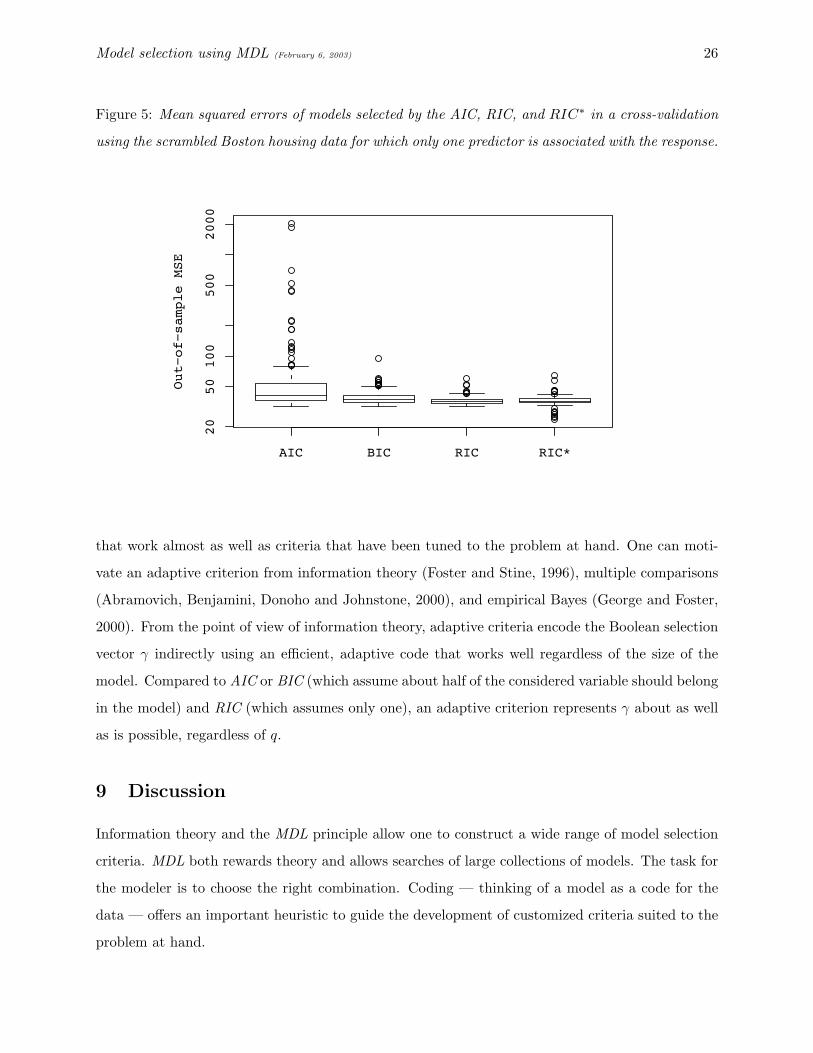
Figure 5: Mean squared errors of models selected by the AIC, RIC, and RIC∗ in a cross-validation

using the scrambled Boston housing data for which only one predictor is associated with the response.

AIC BIC RIC RIC*

2050

100

500

2000

Out−of−sample MSE

that work almost as well as criteria that have been tuned to the problem at hand. One can moti-

vate an adaptive criterion from information theory (Foster and Stine, 1996), multiple comparisons

(Abramovich, Benjamini, Donoho and Johnstone, 2000), and empirical Bayes (George and Foster,

2000). From the point of view of information theory, adaptive criteria encode the Boolean selection

vector γ indirectly using an efficient, adaptive code that works well regardless of the size of the

model. Compared to AIC or BIC (which assume about half of the considered variable should belong

in the model) and RIC (which assumes only one), an adaptive criterion represents γ about as well

as is possible, regardless of q.

9 Discussion

Information theory and the MDL principle allow one to construct a wide range of model selection

criteria. MDL both rewards theory and allows searches of large collections of models. The task for

the modeler is to choose the right combination. Coding — thinking of a model as a code for the

data — offers an important heuristic to guide the development of customized criteria suited to the

problem at hand.


Returning to the question “Which model is best?,” we see that the answer depends on how

we approach the analysis. MDL rewards a theory that generates a model that a less-informed

analyst might need an exhaustive search to discover. The four-predictor regression in Table 2,

when identified a priori, is certainly the best of the illustrative models. Without such a clairvoyant

theory, MDL rates this model highly only if we have chosen to encode the identify of the regression

slopes in a manner suited to searching many possible effects. Again, MDL exploits our knowledge

of the problem at hand, this time in the form of our expectation for how many predictors should

appear in the final model. Codes like those related to the RIC incorporate the notion that the

analyst expects only a few of the searched factors to affect the response. Coding just the index

rather than the long string of bits reflects our expectation of a model with few predictors. Though

the regression tree fairs poorly in this illustration, MDL does allow us to compare it to regression

models.

This discussion of model selection begs the question “What is a model anyway?” Although a

careful answer requires details outside the scope of this paper (e.g. McCullagh, 2002), the essential

properties needed are a likelihood for the data and a “likelihood” for the model as well. This

requirement rules out some popular approaches based on various method-of-moments estimators,

such as GMM. If, however, our theory allows us to express our beliefs asf a probability distribution,

then MDL offers a framework in which we can judge the value of its merits.

One thing that MDL does not ask of us, however, is the existence of a true model. Although

the spike-and-slab formulation leads to a so-called “consistent model selection criterion” (i.e., one

that identifies the true model with probability 1 as the sample size increases), MDL only requires

a probability model for the data. As we have seen, some versions of the MDL behave like AIC and

are thus, like 5% hypothesis tests, not consistent. The better the model that we can write down,

the shorter the code for the data. None have to be the “true model” that generated the data. And,

because the code for the data must describe the model itself, one cannot simply tune the model

ever more closely to a specific sample.

Several reviews of information theory for model selection will be of interest to readers who would

like to learn more about the use of information theory in model selection and statistics. In order

of increasing mathematical sophistication, these are Lee (2001) (which uses polynomial regression

as the motivating example), Bryant and Cordero-Brana (2000) (testing, especially for contingency

tables), Hansen and Yu (2001) (regression and priors), Lanterman (2001) (relationship to Bayesian

methods) and Barron et al. (1998) (coding methods). Rissanen (1989) (Section 3.2) describes the


differences between coding and MDL and the Bayesian approach. As suggested by the number

of citations, the book of Cover and Thomas (1991) gives an excellent introduction to information

theory in general.

Appendix: Estimating σ2

This appendix considers the effects of using an estimate of σ2 when computing description lengths.

The codes described in this paper ignore the fact that σ2 is unknown and must be added to the

code. Since all of the models require such as estimate, adding it as part of the code does not affect

the comparisons. A reduction in the estimated error variance does, however, increase the z-scores of

predictors in the model, and we need to account for this effect. The adjustment essentially replaces

the MLE for σ2 in the likelihood by the familiar unbiased estimator.

Recall that the second part of the two-part code for a regression represents the encoded data.

For a model with q predictors, the MLE for σ2 is

σ2q =

∑i(Yi − β0 − β1X1 − · · ·− βqXq)2

n=

RSS(q)n

. (15)

The description length for the data is then the negative log-likelihood

− log2 L(q) =n

2 ln 2

(1 + ln(2πσ2)

)=

n

2 ln 2ln

RSS(q)RSS(q + 1)

.

Only the leading term affects the comparison of models. The gain in data compression by expanding

a model with q predictors to one with q + 1 is thus

log2 L(q + 1)− log2 L(q) =n

2 ln 2(lnRSS(q)− lnRSS(q + 1)) . (16)

To measure the impact of estimating σ2 on the first part of the code, treat the sequence of

predictors as defining a sequence of orthogonal expansions of the model. The ordered predictors

chosen by forward selection can be converted into an uncorrelated set of predictors, using a method

such as Gram-Schmidt. Further, assume that the resulting orthogonal predictors – which I will

continue to call X1, . . . , Xq – are normalized to have unit length, X ′jXj = 1. Denote the test

statistics for these in a model with q predictors as z0,q, . . . , zq,q for

zj,q = βj/σq ,


and denote those from the model with q + 1 parameters as z0,q+1, . . . , zq,q+1, zq+1,q+1. Because of

orthogonality, only the estimate of the error variance changes in the first q z-scores when Xq+1

joins the model, so

zj,q+1 = zj,qσq

σq+1. (17)

The addition of a predictor then increases the length of the code for the model parameters from

!u(z0,q) + · · ·+ !u(zq,q) to !u(z0,q+1) + · · ·+ !u(zq+1,q+1). If the estimated error variance decreases,

then the test statistics for the first q predictors increase and potentially require longer parameter

codes. We need to capture this effect.

An approximation simplifies the comparison of the description lengths. First, the definition of

the universal length !u(j) given in (11) implies that (ignoring the need for log+2 )

!u(z c) = 2 + log2 z + log2 c + 2 log2(log2 z + log2 c)

= 2 + log2 z + log2 c + 2 log2

(log2(z)

(1 +

log2 c

log2 z

))= log2 z + 2 log2 log2 z + log2 c + 2 log2

(1 +

log2 c

log2 z

).

If c ≈ 1 and z is of moderate size, we can drop the last summand and obtain

!u(z c) ≈ !u(z) + log2 c . (18)

The approximation is justified since we only need it when c = RSS(q)/RSS(q + 1) and z is the

z-score of a predictor in the model (and so is at least 3 to 4).

The approximation (18) leads to an expression for the length of the code for the model param-

eters. Going from a model with q predictors to one with q + 1 increases the length of the model

prefix by about

!u(zq+1,q+1) +q∑

j=0

!u(zj,q+1)− !u(zj,q) = !u(zq+1,q+1) +q∑

j=0

!u(zj,q σq/σq+1)− !u(zj,q)

≈ !u(zq+1,q+1) + (q + 1) log2σq

σq+1

= !u(zq+1,q+1) +q + 12 ln 2

lnRSS(q)

RSS(q + 1). (19)

The MDL principle indicates that one chooses the model with the shorter description length. In this

case, we choose the model with q + 1 predictors if the gain in data compression given in equation

(16) is larger than the increase in the length for the parameters given by (19). That is, we add

Xq+1 to the model if

n

2 ln 2ln

RSS(q)RSS(q + 1)

≥ !u(zq+1,q+1) +q + 12 ln 2

lnRSS(q)

RSS(q + 1),


or equivalently ifn− q − 1

2 ln 2ln

RSS(q)RSS(q + 1)

≥ !u(zq+1,q+1) .

If we assume that the change in fit δ2 = RSS(q)−RSS(q +1) is small relative to RSS(q +1), then

n− q − 12 ln 2

lnRSS(q)

RSS(q + 1)=

n− q − 12 ln 2

lnRSS(q + 1) + δ2

RSS(q + 1)

=n− q − 1

2 ln 2ln(1 + δ2/RSS(q + 1))

≈ n− q − 22 ln 2

δ2

RSS(q + 1)

=1

2 ln 2δ2

s2q+1

=1

2 ln 2t2q+1 ,

where s2q+1 = RSS(q + 1)/(n − q − 2) is the usual unbiased estimate of σ2 and t2q+1 = δ2/s2

q+1 is

the square of the standard t-statistic for the added variable. As a result, the use of the unbiased

estimator s2q allows us to judge the benefit to a model of adding Xj in the same fashion we would

take were we to know σ2.

References

Abramovich, F., Benjamini, Y., Donoho, D. and Johnstone, I. (2000). Adapting to unknown

sparsity by controlling the false discovery rate. Tech. Rep. 2000–19, Dept. of Statistics, Stanford

University, Stanford, CA.

Barron, A. R., Rissanen, J. and Yu, B. (1998). The minimum description length principle in

coding and modeling. IEEE Trans. on Info. Theory 44 2743–2760.

Belsley, D. A., Kuh, E. and Welsch, R. E. (1980). Regression Diagnostics: Identifying

Influential Data and Sources of Collinearity. Wiley, New York.

Breiman, L. and Friedman, J. H. (1985). Estimating optimal transformations for multiple

regression and correlation. Journal of the Amer. Statist. Assoc. 80 580–598.

Breiman, L., Friedman, J. H., Olshen, R. and Stone, C. J. (1984). Classification and

Regression Trees. Wadsworth, Belmon, CA.

Bryant, P. G. and Cordero-Brana, O. I. (2000). Model selection using the minimum descrip-

tion length principle. American Statistician 54 257–268.


Cover, T. M. and Thomas, J. A. (1991). Elements of Information Theory. Wiley, New York.

Elias, P. (1975). Universal codeword sets and representations of the integers. IEEE Trans. on

Info. Theory 21 194–203.

Foster, D. P. and George, E. I. (1994). The risk inflation criterion for multiple regression.

Annals of Statistics 22 1947–1975.

Foster, D. P. and Stine, R. A. (1996). Variable selection via information theory. Tech. Rep.

Discussion Paper 1180, Center for Mathematical Studies in Economics and Management Science,

Northwestern University, Chicago.

Foster, D. P. and Stine, R. A. (1999). Local asymptotic coding. IEEE Trans. on Info. Theory

45 1289–1293.

Foster, D. P. and Stine, R. A. (2002). Variable selection in data mining: Building a predictive

model for bankruptcy. Submitted for publication.

Foster, D. R. and Stine, R. A. (2003). The boundary between parameters and data in stochastic

complexity. In P. Grunwald, I. J. Myung and M. Pitt, eds., Advances in Minimum Description

Length: Theory and Applications. MIT Press, to appear.

Fox, J. (1984). Linear Statistical Models and Related Methods with Applications to Social Research.

Wiley, New York.

George, E. I. and Foster, D. P. (2000). Calibration and empirical bayes variable selection.

Biometrika 87 731–747.

Hansen, M. H. and Yu, B. (2001). Model selection and the principle of minimum description

length. Journal of the Amer. Statist. Assoc. 96 746–774.

Harrison, D. and Rubinfeld, D. L. (1978). Hedonic prices and demand for clean air. J. of

Environmental Economics and Management 5 81–102.

Hinkley, D. V. (1970). Inference about the change-point in a sequence of random variables.

Biometrika 57 1–17.

Langdon, G. G. (1984). An introduction to arithmetic coding. IBM Journal of Research and

Development 28 135–149.


Lanterman, A. D. (2001). Schwarz, Wallace, and Rissanen: Intertwining themes in theories of

model selection. International Statistical Review 69 185–212.

Lee, T. C. M. (2001). An introduction to coding theory and the two-part minimum description

length principle. International Statistical Review 69 169–183.

Manish, M., Rissanen, J. and Agrawal, R. (1995). MDL-based decision tree pruning. In

Proceedings of the First International Conference on Knowledge Discovery and Data Mining

(KDD’95).

McCullagh, P. (2002). What is a statistical model? Annals of Statistics 30 1225–1310.

Miller, A. J. (2002). Subset Selection in Regression (Second Edition). Chapman& Hall, London.

Rissanen, J. (1978). Modeling by shortest data description. Automatica 14 465–471.

Rissanen, J. (1983). A universal prior for integers and estimation by minimum description length.

Annals of Statistics 11 416–431.

Rissanen, J. (1986). Stochastic complexity and modeling. Annals of Statistics 14 1080–1100.

Rissanen, J. (1989). Stochastic Complexity in Statistical Inquiry. World Scientific, Singapore.

Rissanen, J. and Wax, M. (1988). Algorithm for constructing tree structured classifiers. Tech.

Rep. No. 4,719,571, U.S. Patent Office, Washington, DC.

Venables, W. N. and Ripley, B. D. (2002). Modern Applied Statistics with S-PLUS. Springer,

New York, fourth edition ed.

M odel Selection using Inform ation T heory and …stine/research/smr.pdfM odel Selection using...

Documents

Transcript of M odel Selection using Inform ation T heory and …stine/research/smr.pdfM odel Selection using...