^LZ77^AA,V^ - ttu-ir.tdl.org
73
SOLAR CONCENTRATOR WIND LOADINGS by GEOFFREY L. WAGNER, B.S.M.E. A THESIS IN MECHANICAL ENGINEERING Submitted to the Graduate Faculty of Texas Tech University in Partial FulfiUment of the Requirements for the Degree of MASTER OF SCIENCE IN MECHANICAL ENGINEERING Approved Chaj^erson of the Committee <r ^LZ77^AA,V^ ^ Accepted ^^^f/^^J^U. Dean of the Gr December, 1996
Transcript of ^LZ77^AA,V^ - ttu-ir.tdl.org
SOLAR CONCENTRATOR WIND LOADINGS
by
GEOFFREY L. WAGNER, B.S.M.E.
A THESIS
IN
MECHANICAL ENGINEERING
Submitted to the Graduate Faculty of Texas Tech University in
Partial FulfiUment of the Requirements for
the Degree of
MASTER OF SCIENCE
IN
MECHANICAL ENGINEERING
Approved
Chaj^erson of the Committee
<r ^LZ77^AA,V^
^
Accepted
^^^f/^^J^U. Dean of the Gr
December, 1996

ACKNOWLEDGMENTS
Q. ' ^ I would like to extend my special thanks to Dr. Jerry Dunn for all his
help and insight. Without his guidance and assistance this work would not
have been possible. I would also Uke to extend my thanks to Dr. Ertas and
Dr. Oler for their time and expertise as members of my thesis committee.
Your assistance and encouragement helped me to get through my thesis. My
special thanks goes Cummins Power Generation for the support of the project
and for the assistance and direction given throughout the project.
I also would like to extend a warm thank you to my family and friends
that always encouraged me throughout this ordeal. My family has always
been behind me whether it be moral or financial support so I could not have
made it through without them. Thanks also goes to RocheUe Pritchard for
the help on the project, from the beginning to the end. I could not have
finished the project without you. In addition, Uoyd Lacy was a large
contributor to the project through his assistance in the machining and
materials advice.
Most importantly, I would like to thank the Lord for His grace and
mercy. His guidance carried me through the project and without Him, I am
nothing.
11
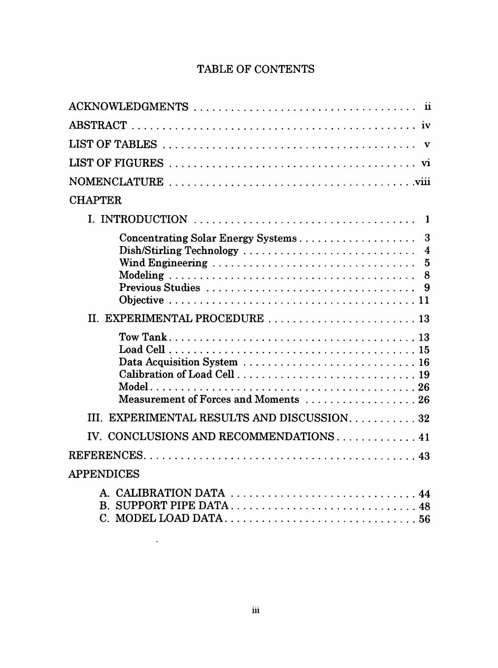
TABLE OF CONTENTS
ACKNOWLEDGMENTS ii
ABSTRACT iv
LIST OF TABLES v
LIST OF FIGURES vi
NOMENCLATURE viii
CHAPTER
I. INTRODUCTION 1
Concentrating Solar Energy Systems 3 Dish/Stirhng Technology 4 Wind Engineering 5 Modeling 8 Previous Studies 9 Objective 11
n. EXPERIMENTAL PROCEDURE 13
Tow Tank 13 Load Cell 15 Data Acquisition System 16 Calibration of Load Cell 19 Model 26 Measurement of Forces and Moments 26
m . EXPERIMENTAL RESULTS AND DISCUSSION 32
IV. CONCLUSIONS AND RECOMMENDATIONS 41
REFERENCES 43
APPENDICES
A. CALIBRATION DATA 44 B. SUPPORT PIPE DATA 48 C. MODEL LOAD DATA 56
111

ABSTRACT
The objective of this project was to determine the maximum wind
loadings on a notched parabohc solar concentrator. To accomplish this
objective, a test program was conducted using the Texas Tech tow tank. The
results from testing a one-tenth scale model were put into nondimensional
force and moment coefficients. The maximum coefficients are as follows: hft,
-0.92; drag, 1.42; side force, 1.05; yaw moment, -0.23; roU moment, 0.72; and
pitch moment, 1.28. These results shovdd be used as a starting estimate for
the beginning stages of the structural design of the solar concentrator
support structure.
IV
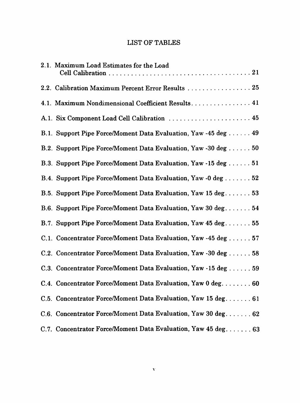
LIST OF TABLES
2.1. Maximum Load Estimates for the Load
CeU CaHbration 21
2.2. Calibration Maximum Percent Error Results 25
4.1. Maximum Nondimensional Coefficient Results 41
A.I. Six Component Load Cell Calibration 45
B.l. Support Pipe Force/Moment Data Evaluation, Yaw -45 deg 49
B.2. Support Pipe Force/Moment Data Evaluation, Yaw -30 deg 50
B.3. Support Pipe Force/Moment Data Evaluation, Yaw -15 deg 51
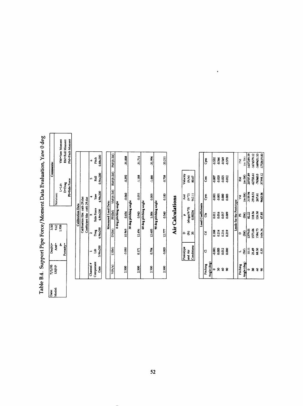
B.4. Support Pipe Force/Moment Data Evaluation, Yaw -0 deg 52
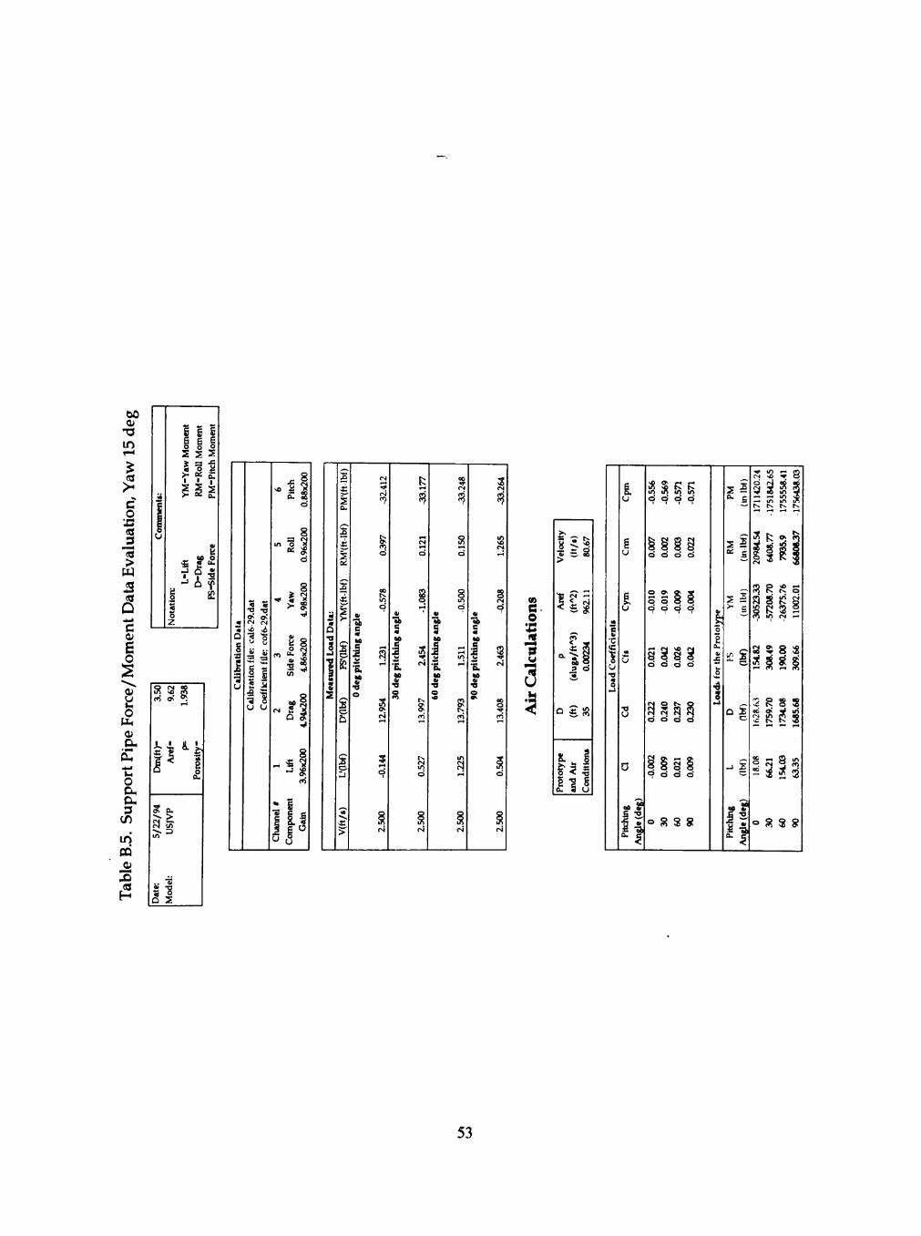
B.5. Support Pipe Force/Moment Data Evaluation, Yaw 15 deg 53
B.6. Support Pipe Force/Moment Data Evaluation, Yaw 30 deg 54
B.7. Support Pipe Force/Moment Data Evaluation, Yaw 45 deg 55
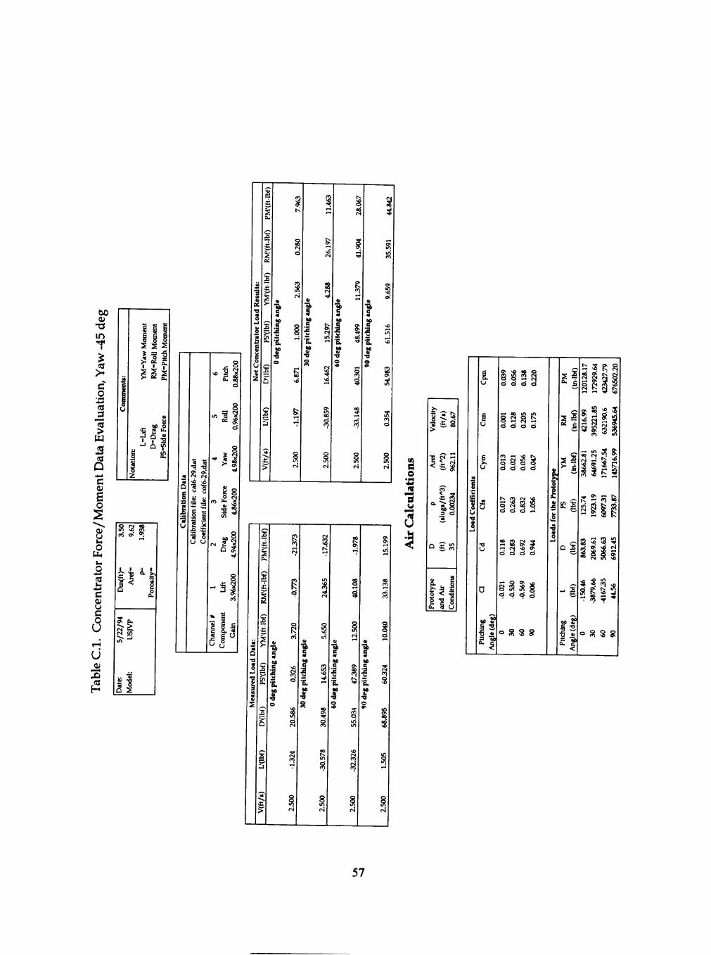
C.l. Concentrator Force/Moment Data Evaluation, Yaw -45 deg 57
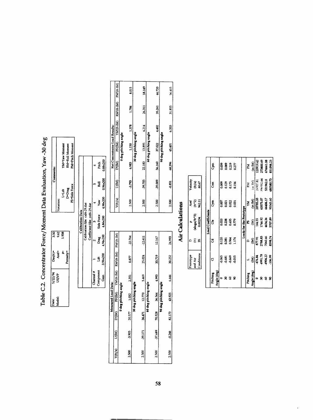
C.2. Concentrator Force/Moment Data Evaluation, Yaw -30 deg 58
C.3. Concentrator Force/Moment Data Evaluation, Yaw -15 deg 59
C.4. Concentrator Force/Moment Data Evaluation, Yaw 0 deg 60
C.5. Concentrator Force/Moment Data Evaluation, Yaw 15 deg 61
C.6. Concentrator Force/Moment Data Evaluation, Yaw 30 deg 62
C.7. Concentrator Force/Moment Data Evaluation, Yaw 45 deg 63
\

LIST OF FIGURES
1.1. Cummins Power Generation 25 kW Solar Concentrating System 2
1.2. Direction of Forces and Angles Relative to the Wind Direction 7
1.3. One-tenth Scale Model of Cummins Power
Generation 25 kW Solar Concentrator 12
2.1. Texas Tech's Tow Tank Facility 14
2.2. Load CeU Illustration 15
2.3. Wheatstone Bridge Configuration 16
2.4. Data Acquisition System 17
2.5. Measurements Group Model 2100 Strain
Gage Amplifier 17
2.6. Controls to Balance Bridges and Setting the Gain 18
2.7. Calibration Setup 20
2.8. Lift Calibration Curve 22
2.9. Drag Calibration Curve 22
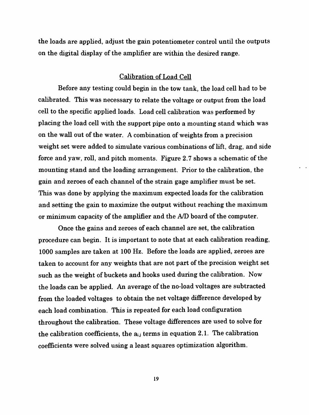
2.10. Side Force Calibration Curve 23
2.11. Yaw Moment Calibration Curve 23
2.12. Roll Moment Calibration Curve 24
2.13. Pitch Moment Calibration Curve 24
2.14. One-tenth Scale Model of Solar Concentrator 27
M
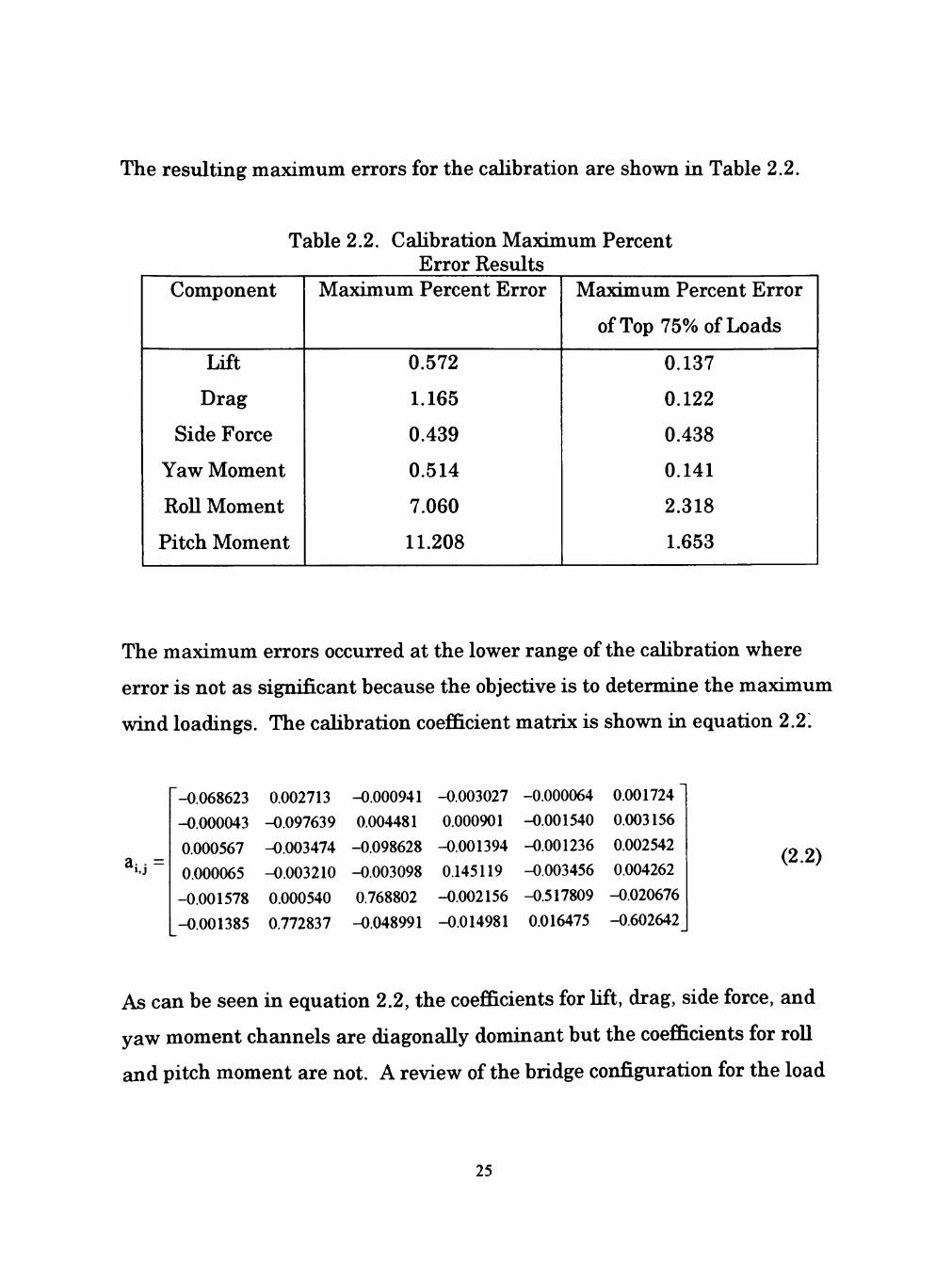
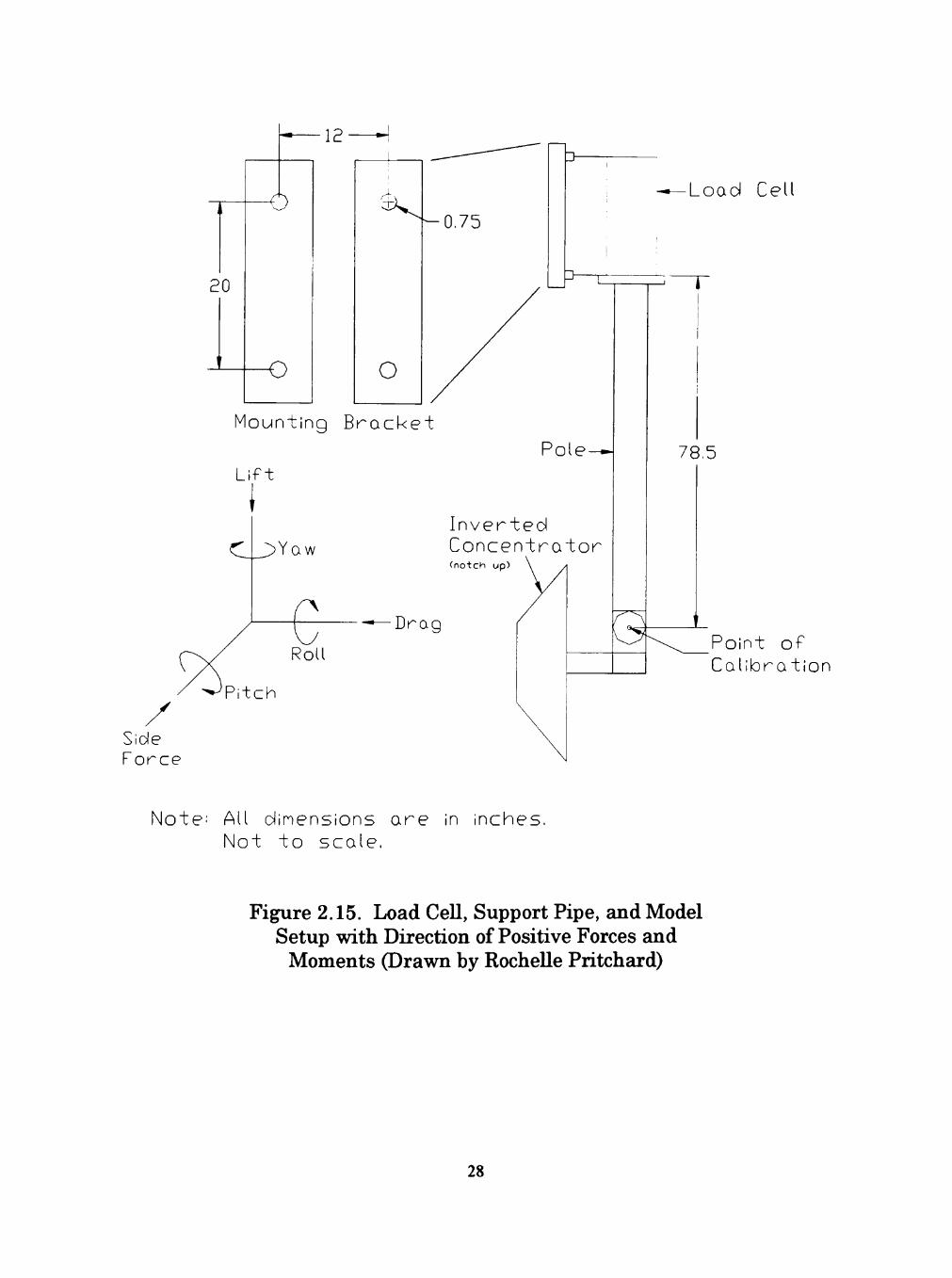
2.15. Load CeU, Support Pipe, and Model Setup with Direction of Positive Forces and Moments 28
2.16. Yaw Angles and Direction of Positive Forces
and Moments 29
3.1. Lift Coefficients for Varying Yaw Angles 33
3.2. Drag Coefficients for Varying Yaw Angles 33
3.3. Side Force Coefficients for Varying Yaw Angles 34
3.4. Yaw Coefficients for Varjdng Yaw Angles 34
3.5. RoU Coefficients for Varying Yaw Angles 35
3.6. Pitch Coefficients for Varying Yaw Angles 35
vu

NOMENCLATURE
A
aij
^
ap
ar
CD
CF
CL
CM
CpM
CRM
CsF
CYM
d
D
F
f
FD ,Di
FL,Li
FsF, SFi
t-Tnodel
t-prototype
t^ratio
MpM , Pi
MRM,Ri
MYM , Yi
Characteristic area
Calibration coefficients
Acceleration of model
Acceleration of prototype
Acceleration ratio
Drag coefficient
Force coefficient
Lift coefficient
Moment coefficient
Pitching moment coefficient
Rolling moment coefficient
Side coefficient
Yawing moment coefficient
Characteristic diameter
Aperture diameter
Force
Focal length
Drag force
Lift force
Side force
Length of model
Length of prototype
Length ratio
Pitching moment
Rolling moment
Yawing moment
Vlll
q
Qm
Qp
Qr
P
Re
Rem
Rcp
Tn,
Tp
T.
V
Voi
Vu
Vn,
Vp
Vpi
V.
VRI
VsFi
Vvi
Dynamic pressure
Volumetric flow rate of model
Volumetric flow rate of prototype *
Volumetric flow rate ratio
Fluid density
Reynolds number
Reynolds number of model
Reynolds number of prototype
Time of model
Time of prototype
Time ratio
Wind velocity
Vohage due to drag force
Voltage due to lift force
Velocity of model
Velocity of prototype
Voltage due to pitching moment
Velocity ratio
Voltage due to rolling moment
Voltage due to side force
Voltage due to yawing moment
IX

CHAPTER I
INTRODUCTION
For the past twenty years, efficient energy management and effective
conservation procedures have been very important considerations for our
society. An oU embargo in the 1970s and early 1980s combined with various
circumstances such as the loss of tax credits and new efficiency standards
imposed by the government brought about a new awareness concerning
energy. The Clean Air Act of 1991 and the Persian Gulf War have spurred a
revival in the need for reUable and environmentaUy friendly energy sources.
One possibility for a renewable energy source is that of solar energy
coUectors.
A United States Joint Venture Program (USJVP) is making an effort
to increase the feasibility of solar coUecting systems. Numerous companies
have been concentrating their efforts in dish/Stirling concentrator
technology. There has already been developed a 7.5-kW free-piston engine
dish/Stirling system and through the efforts of the joint venture program the
development and testing of a 25-kW kinematic-piston Stirling engine, shown
in Figure 1.1, for terrestrial power generation. Some of the controlling
factors in determining the size and power generation of solar concentrators
are the engines and the wind loads on the support structures. With regard to
wind loading, the wind loads affect the accuracy of the reflector as a
paraboloid, pointing accuracy, loads on the drive system, safety in extreme
winds, and freedom from osciUations (Wyatt, 1964). In an effort to determine
the mean wind loads of a 25-kW concentrator, testing of a scale model
concentrator was carried out by Texas Tech University Department of
Mechanical Engineering.

Figure 1.1. Cummins Power Generation 25 kW Solar Concentrating System

Concentrating Solar Energy Systems
Most of the solar energy research done in the past few years has been
focused on intermediate to high temperature technologies, which includes
solar energy concentrating systems. Solar coUectors are essentiaUy heat
exchangers which can vary widely in design and types. Two main
classifications are concentrating and nonconcentrating systems. Their
general design geometry can be cylindrical or paraboloidal, and can be
continuous or faceted. Concentrating coUectors are classffied by their
tracking requirements which can be one-axis tracking, two-axis-tracking or
non-tracking systems. Because concentrating coUectors focus solar radiation,
they provide energy at temperatures higher than that provided by flat-plate
coUectors. The focused solar radiation passes through an aperture onto an
absorber which usuadly requires tracking of the sun. In most concentrating
systems, the concentrated Ught is used to heat a fluid as a source for a
generator. The working fluid is usuaUy a Hquid (plain water), oU, gas (air) or
black Uquids (water and Indian ink mixture) which can use a transparent
glass tube instead of a black-coated copper tube as the receiver (Imadojemu,
1995). Other concentrators use dish-mounted Rankine, Brayton, or StirUng
cycle engines to produce electric power.
One factor that determines the effectiveness of concentrators is the
concentration ratio. Concentration ratios can vary from values sHghtly
greater than unity to high values of the order of 10 . The concentration ratio
is defined as the ratio of the coUector aperture area to the absorber area. As
the ratio increases, the operating temperature increases which emphasizes
the importance of precision in optical quaUty and positioning of the optical
system.

Solar energy usage has enormous potential for a conservation minded
friture. Electricity can be generated through heat coUection/conversion or
from photo conversion. Other uses for solar energy include the production of
fuels and chemical processes, space heating, wood or vegetable drying, and
solar cooking (Imadojemu, 1995).
Dish/Stirling Technology
Solar concentrators and StirUng engines are a perfect match because
concentrators provide the high temperatures needed for power production
from the Stirling engine. A Scottish minister. Rev. Robert StirUng, patented
the Stirling engine in 1816 and the first solar appUcation was by the famous
British/American inventor John Ericsson in 1872. The StirUng engine is the
most efficient device for converting heat into mechanical work (Stine, 1993).
A high efficiency StirUng engine results in more output for a given size
concentrator. To the consumer, this means lower cost electricity. StirUng
engine efficiency increases with operating temperature; and therefore, these
devices are operated up to the thermal limits of the materials used in their
construction. Engine conversion efficiencies are around 30 to 40% for a
temperature range of 650° to 800°C (1200° to 1470°F) (Stine and Diver,
1994). The engines typicaUy operate at high pressure, 5 to 20 MPa (725 to
2900 psi), to maximize the power output (Stine and Diver, 1994).
In order to obtain the high temperatures that are required for StirUng
concentrators, tracking the sun is necessary. Tracking mechanisms are very
expensive and are very sensitive because variations in tracking accuracy can
result in a large increase in temperature, conversely, inaccuracy in the
tracking system could cause lower efficiencies. In addition, inaccuracies
could result in faUure of the receiver because temperatures could be greater

than the thermal Umits of materials not designed to be operated at high
levels of solar heat flux. The largesT mechanical loads on the tracking
mechanisms are those caused by the wind. Therefore, knowing the mean
wind loads is critical in designing the tracking systems for Stirling
concentrators.
Wind Engineering
Wind is caused by atmospheric pressure differences that arise from
unequal heating of the Earth's surface. Some of the important factors that
influence the wind include the Earth's rotation, precipitation, cloud cover,
non-uniform surface temperature and roughness, and topographic reUef
(Roschke, 1984). It is because of the variabUity and randomness of these
factors that makes it very chaUenging to characterize wind mathematicaUy.
The need for wind engineering comes from the fact that moderate to strong
wind conditions can cause extensive damage to structures.
One of the purposes of wind engineering is to determine the resultant
wind forces and moments. By applying BernouUi's principle and dimensional
analysis, the wind force and moment can be expressed in the form of
equations 1.1 and 1.2
F = lpV^ACp (1.1)
M = ipV^AdC^ (1.2)
where p is the mass density of the airstream, V is the wind velocity, A is a
characteristic area of the body, d is a characteristic dimension of the body,

and CF and CM are the dimensionless force and moment coefficients. The
dimensionless coefficients depend on the geometric properties of the body and
on Reynolds number. The term V2pV2 is the dynamic pressure of the
undisturbed flow and is designated as q.
In aerodynamics, the force is usuaUy separated into the three
orthogonal forces of drag, Uft, and side force. Their corresponding coefficients
are CD, CL, and CSF. The moment may also be broken into three orthogonal
moments of yaw, roU, and pitching moments with corresponding coefficients
of CYM, CRM, and CPM. These aerodynamic forces and moments are expressed
in equation form in equations 1.3 through 1.8.
Lift: FL= CL-qA (1.3)
Drag: FD = CoqA (1.4)
Side Force: FSF = CsF-qA (1.5)
Yawing Moment: MYM = CYMdqA (1.6)
RoUingMoment: MRM= CRM-dqA (1.7)
Pitching Moment: MpM=CpMdqA (1.8)
It is important to note that the positive direction of the forces is fixed
relative to the wind direction. Figure 1.2 shows the direction of the forces
relative to the wind direction as weU as the yaw, roU, and pitch angles. Drag
is in the horizontal direction paraUel to the wind and the positive direction is
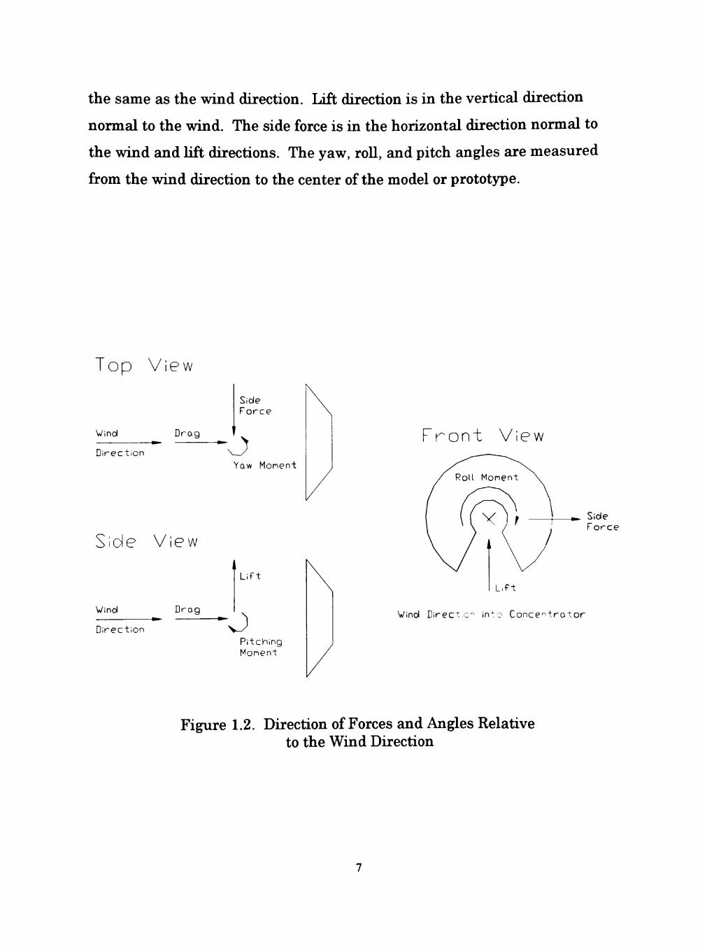
the same as the wind direction. lift direction is in the vertical direction
normal to the wind. The side force is in the horizontal direction normal to
the wind and Uft directions. The yaw, roU, and pitch angles are measured
from the wind direction to the center of the model or prototype.
Top
Wind
D i r e c t i o n
View
Drag 1
Side F o r c e
J Yaw Monent
Side View
Wind
D i r e c t i o n
D r a g
L i f t
O Pi tch ing Monent
F r o n t View
L , f t
Wind D i r ec t , c ^ in^o C o n c e n t r o t o r
Figure 1.2. Direction of Forces and Angles Relative to the Wind Direction

Modeling
Sometimes it is necessary to determine the performance of a structure
through experimental testing of another structure. This is caUed model
testing where the structure being tested is the model and the structure whose
performance is being predicted is the prototype. It is possible for the model
to be smaUer than, the same size as, or even larger than the prototype.
Model experiments of structures have resulted in savings that more than
justified the expenditures of funds for the design, construction, and testing of
the model.
In order for the model and prototype to have similar results, it is
necessary to have geometric, kinematic, and d5niamic simdarity. When the
ratios of aU the corresponding dimensions of the model and the prototype are
equal, it is caUed geometric similarity. These ratios are written in equations
1.9 through 1.11:
Length: 'model
'prototype ~ ^r«tio (1.9)
Area:
Volume:
LJ model
l-< prototype
T 3 LJ model
1-1 prototype
— T 2 . 1^ ntio
T 3 i~) ratio
(1.10)
(1.11)
Kinematic simUarity exists between model and prototype when their
streamlines are geometricaUy sinular. The kinematic ratios from this
condition are shown in equations 1.12 to 1.14.
8

Acceleration: a =?^ = hiL^ (1.12) a„ L T"
p p p
Velocity: V = ^ = 1IHIE_ (1.13) ' V„ L T-'
p p p
O L T ' Volume flow rate: Q =-^= " " (1.14)
' Q„ L' T ' ^ p p p
Dynamic simdarity exists between model and prototype having
geometric and kinematic simdarity when the ratios of aU forces are the same.
For dynamic simUarity, the Reynolds numbers must be equal as shown in
equations 1.15 and 1.16.
pLV Reynolds number Re = (115)
Re„=Rep (1.16)
Previous Studies
Several previous studies have been conducted on wind loadings on
solar concentrators. There is general agreement that wind loads influence
the design, performance, cost, safety, and maintenance and replacement costs
of solar concentrators. Wind loads are functions of wind conditions and the
design and configuration of the concentrator. As shown above, the force and
moments are functions of the square of the mean wind velocity as weU as the

concentrator diameter. Drag force increases as the pitching angle increases
to a maximum of 90°. In addition to drag force, the wind forces and moments
can vary considerably with wind angle of attack and can be either positive or
negative.
E.J. Roshke (1984) has made several general conclusions about wind
loadings on solar concentrators. Roshke stresses that the annual energy
production is related to the wind conditions, which are therefore important to
the design of the concentrator. Roshke points out that there are several
methods to reduce wind loads including introducing or increasing the
porosity of the concentrator, the use of spoUers and fairings, and shifting the
point of rotation forward of the dish vertex. Roshke also notes that to avoid
scale effects, Reynolds numbers must be greater than 10 and preferably 10
(Roshke, 1984).
L.M. Murphy (1981) has made several observations about how solar
coUectors are affected by wind loadings. Murphy has noted that wind forces
are difficult to model because the coUector moves to track the sun. Murphy
(1981) also points out that the pointing accuracy and survival are crucial
design factors, but the slew-to-stow condition is the major design motivator.
Murphy Usts the criteria for the design of solar dishes as the maximum
survival wind speed of 100 mph, design wind speed for normal operation of
36 mph, maximum wind speed during which the coUector must track of 36
mph, and a 100 j ^ mean recurrence interval. Murphy notes that Colorado
State University states that there is a diminishing effect of Reynolds
numbers for Re > 15,000. Murphy also Usts the maximum force and moment
coefficients for a dish coUector with a 75° rim angle and a dish
depth/diameter ratio of 0.2. The results were a maximum drag coefficient of
10
1.5, maximum Uft coefficient of 0.25-0.30, and a maximum pitching moment
coefficient of-0.05 at a pitch angle of 40° (Murphy, 1981).
Objective
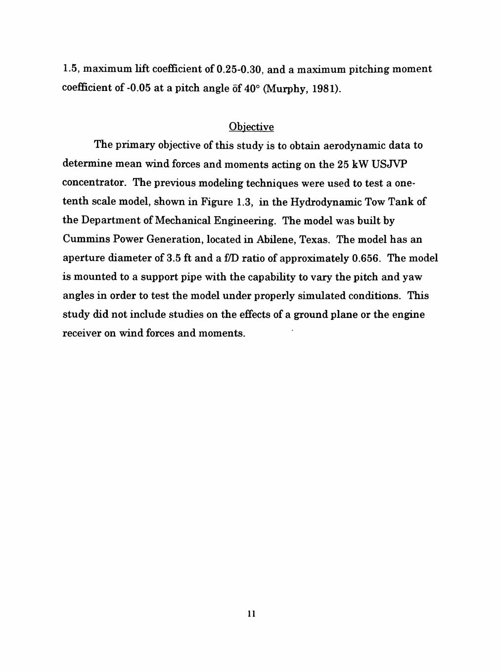
The primary objective of this study is to obtain aerodynamic data to
determine mean wind forces and moments acting on the 25 kW USJVP
concentrator. The previous modeUng techniques were used to test a one-
tenth scale model, shown in Figure 1.3, in the Hydrod5niamic Tow Tank of
the Department of Mechanical Engineering. The model was bmlt by
Cummins Power Generation, located in AbUene, Texas. The model has an
aperture diameter of 3.5 ft and a {/D ratio of approximately 0.656. The model
is mounted to a support pipe with the capabUity to vary the pitch and yaw
angles in order to test the model under properly simulated conditions. This
study did not include studies on the effects of a ground plane or the engine
receiver on wind forces and moments.
11

Figure 1.3. One-tenth Scale Model of Cummins Power Generation 25 kW Solar Concentrator
12

CHAPTER II
EXPERIMENTAL PROCEDURE
In order to complete the objectives of this project, the experiment was
divided into sections where each section must be accompUshed prior to
beginning the next. The first step in the experiment was to become familiar
with the tow tank facUity and measuring equipment. This equipment
included the load ceU and the data acquisition system. The next major step
in the experiment was to caUbrate the load ceU in order to accurately
measure the wind loads appUed to the model. The last step was to perform
the testing of the model in the tow tank.
Tow Tank
The tow tank faciUty at Texas Tech is used to measure aerodynamic
loading and characteristics of large models. The tow tank has the advantage
of being able to test the model at a slower velocity to obtain the same
Reynolds number as in air. Another advantage is that larger models can be
tested in the tow tank than in the Texas Tech wind tunnel. The tow tank is
15 ft wide, 10 ft deep, and 80 ft long and is shown in Figure 2.1. RaUs are
attached to the waUs of the tow tank along the 80 ft span. The raUs support
a moving bridge which spans the tow tank and houses the bridge motor,
computer, strain gage amplifier, bridge control panel, video equipment, and
load ceU. The bridge is able to push or puU models through the water at a
velocity of 0 to 5 feet per second, depending on the model size and the
capabUity of the load ceU. The temperature of the water is approximately 67"=
F year around. The facUity has the capabiUty of providing flow visualization
13
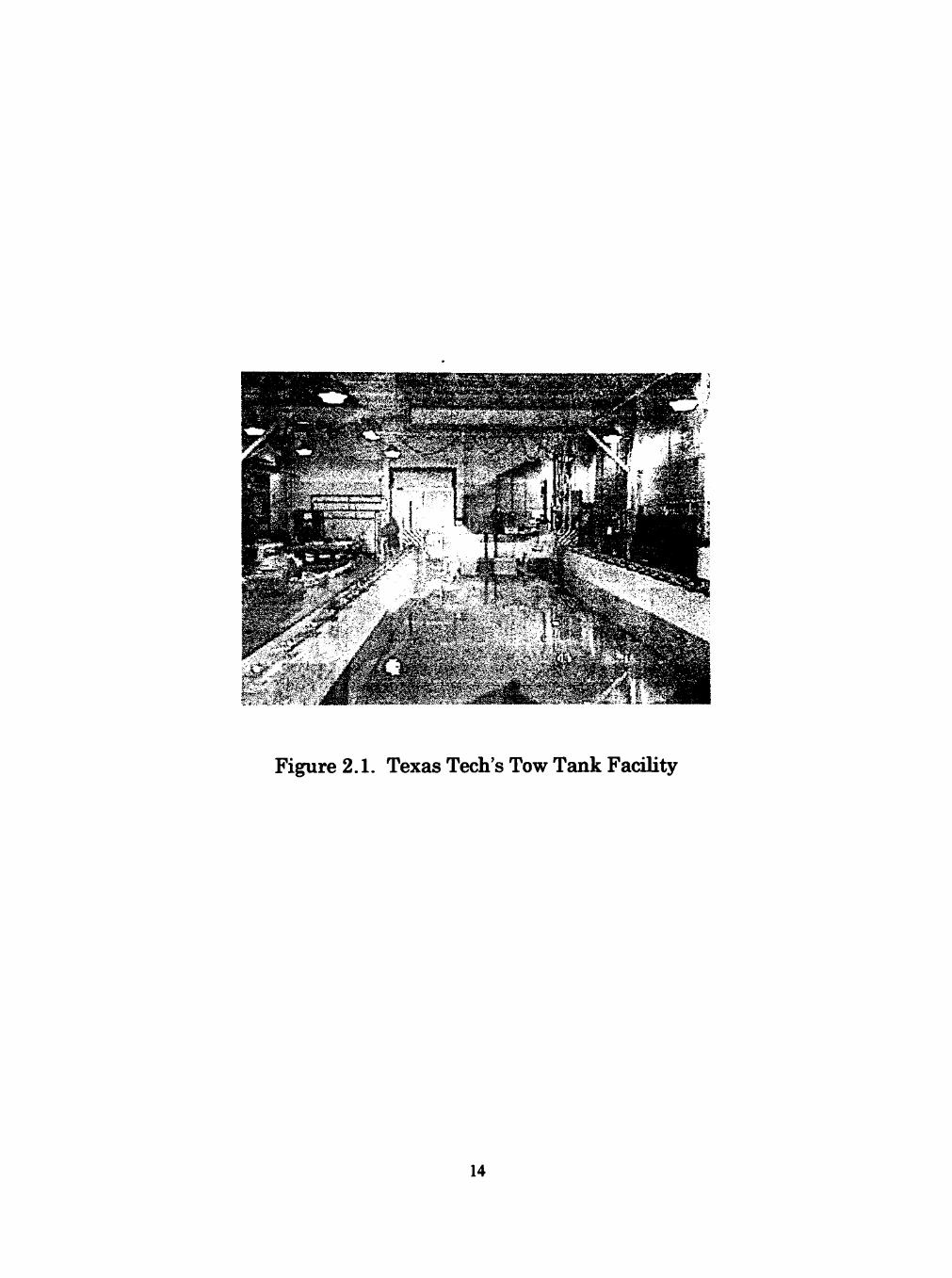
Figure 2.1. Texas Tech's Tow Tank FaciUty
14

using a dye system that injects food dye into the water which can be recorded
using special video cameras that can be located at any depth in the water
Load CeU
The load ceU is the instrument that is used to measure loads on the
models. The load ceU was buUt by Casey Osborne under the supervision of
Dr. J.W. Oler. An Ulustration of the load ceU is shown in Figure 2.2. The
load ceU uses strain gages to provide a voltage output proportional to the
appUed loads. Strain gages are used because their resistance changes as the
appUed strain changes. Since strain gages are sensitive to temperatures, the
readings are compensated by connecting four gages into a Wheatstone bridge
circuit (Figure 2.3). In this configuration, the temperature effects are
canceUed. The load ceU is designed to measure aU six components of force
and moments and has 24 strain gages in 6 Wheatstone bridge circuits, one
for each force and moment.
Lift Gages
Yaw Monent Gages
Drag Gages P i tch Monent Gages
Side Fo rce Gages
J r-f\^—Roll Monent Gages
Figure 2.2. Load CeU lUustration
15
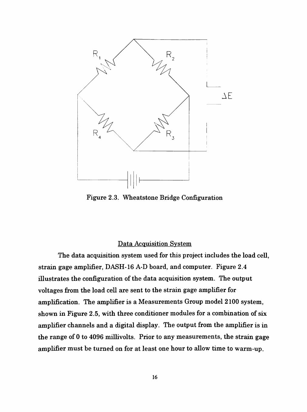
Figure 2.3. Wheatstone Bridge Configuration
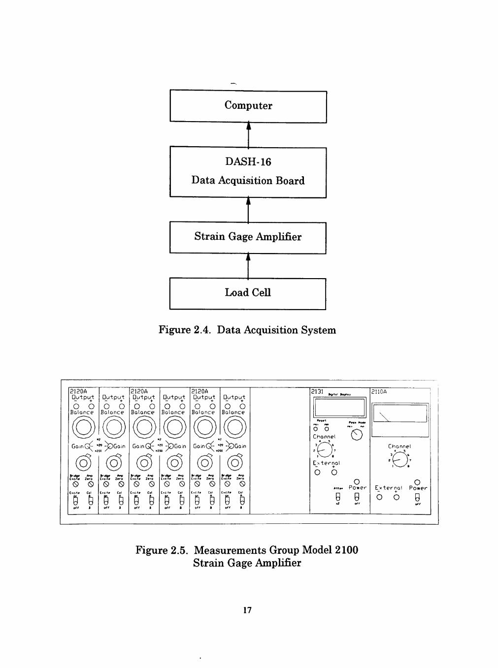
Data Acquisition System
The data acquisition system used for this project includes the load ceU,
strain gage amplifier, DASH-16 A-D board, and computer. Figure 2.4
Ulustrates the configuration of the data acquisition system. The output
voltages from the load ceU are sent to the strain gage amplifier for
amplification. The amplifier is a Measurements Group model 2100 system,
shown in Figure 2.5, with three conditioner modules for a combination of six
ampUfier channels and a digital display. The output from the amplifier is in
the range of 0 to 4096 mUUvolts. Prior to any measurements, the strain gage
amplifier must be turned on for at least one hour to aUow time to warm-up.
16
Computer
1
DASH-16
Data Acquisition Board
Strain Gage AmpUfier
1
Load CeU
Figure 2.4. Data Acquisition System
2120A Output
o o Balonce
Output
o o Bolonce
Citcrt* Z#ro
G G C>c.<> Col C.c.-t* Col
B B
2120A Output
o o Balance
Output
o o Bolonce
GoinGb "' ^ G o i n
Cxcilv 7»ro
G G C>c.t< Col
e B
Br->dgr Anp
G G [•c,1» Col
2120A Output
o o Bolonce
Output
o o Bolonce
^ \ .goo /
E»c.1» Z»ro
G G t»c.-t» Col
B A
0
Br,dO» Anp
G G Cxc.lr Col
B B
2131 IhQi1«< Sisp<*v
o o Chonnel 3 /
o Ex-ternol
6 6 o
•«»« Power
5 0
2nOA
Chonnel
•D: O
Externa l Power
o o 0
Figure 2.5. Measurements Group Model 2100 Strain Gage AmpUfier
17
The output is sent to the DASH-16 data acquisition board inside the
computer. A program written by Dr. Oler is used to read the signal from the
board to determine the resultant loads.
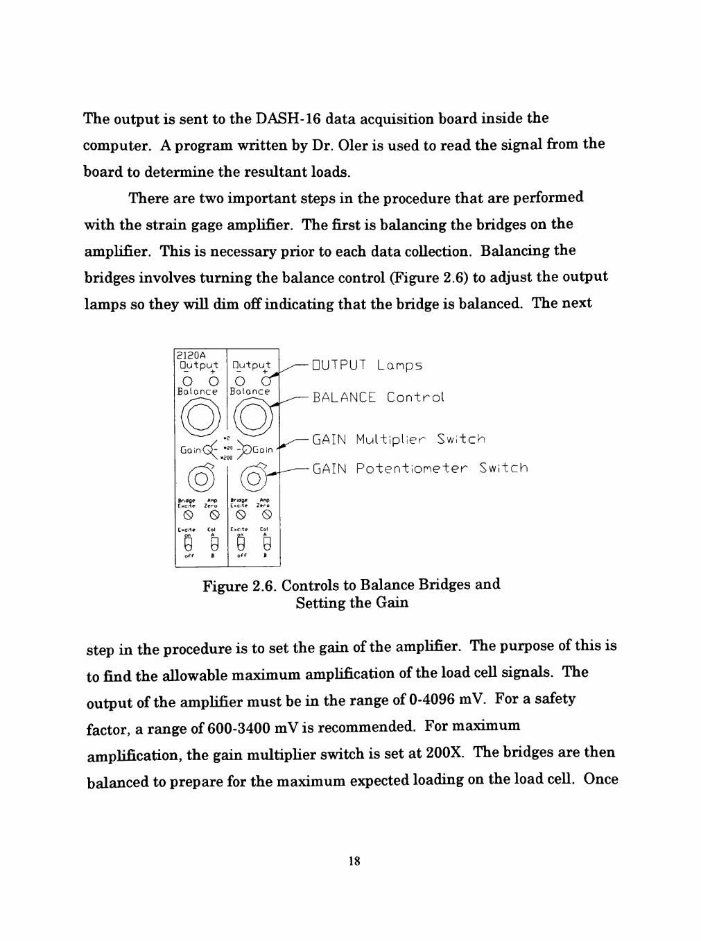
There are two important steps in the procedure that are performed
with the strain gage amplifier. The first is balancing the bridges on the
ampUfier. This is necessary prior to each data coUection. Balancing the
bridges involves turning the balance control (Figure 2.6) to adjust the output
lamps so they wUl dim off indicating that the bridge is balanced. The next
ai20A Output
o o Balance
DutpuJ;
6 Balance
GainG^ "" -feCo in
Br.dge Anp
Exci-t* Zero
G G Exci-tff Col
on A
g B
Bridge ^r*P
E)'Ci*e Z e r o
G G E«citp Col
on A 0 s
OUTPUT L a n p s
BALANCE C o n t r o l
GAIN Mu l t i p l i e r Sw i t ch
GAIN P o t e n t i o n e t e r Sw i t ch
Figure 2.6. Controls to Balance Bridges and Setting the Gain
step in the procedure is to set the gain of the amplifier. The purpose of this is
to find the aUowable maximum amplification of the load ceU signals. The
output of the amplifier must be in the range of 0-4096 mV. For a safety
factor, a range of 600-3400 mV is recommended. For maximum
amplification, the gain multipUer switch is set at 200X. The bridges are then
balanced to prepare for the maximum expected loading on the load ceU. Once
18
the loads are appUed, adjust the gain potentiometer control untU the outputs
on the digital display of the amplifier are within the desired range.
CaUbration of Load CeU
Before any testing could begin in the tow tank, the load ceU had to be
caUbrated. This was necessary to relate the yoltage or output from the load
ceU to the specific appUed loads. Load ceU caUbration was performed by
placing the load ceU with the support pipe onto a mounting stand which was
on the waU out of the water. A combination of weights from a precision
weight set were added to simulate yarious combinations of lift, drag, and side
force and yaw, roU, and pitch moments. Figure 2.7 shows a schematic of the
mounting stand and the loading arrangement. Prior to the caUbration, the
gain and zeroes of each channel of the strain gage ampUfier must be set.
This was done by applying the maximum expected loads for the caUbration
and setting the gain to maximize the output without reaching the maximum
or minimum capacity of the ampUfier and the A/D board of the computer.
Once the gains and zeroes of each channel are set, the caUbration
procedure can begin. It is important to note that at each caUbration reading,
1000 samples are taken at 100 Hz. Before the loads are appUed, zeroes are
taken to account for any weights that are not part of the precision weight set
such as the weight of buckets and hooks used during the caUbration. Now
the loads can be appUed. An ayerage of the no-load yoltages are subtracted
from the loaded yoltages to obtain the net yoltage difference deyeloped by
each load combination. This is repeated for each load configuration
throughout the caUbration. These yoltage differences are used to solye for
the caUbration coefficients, the aij terms in equation 2.1. The caUbration
coefficients were solyed using a least squares optimization algorithm.
19

Yaw Monent
Support Pole
Drag
L i f t and Roil Monent
L i f t and P i t ch Monent
T
Figure 2.7. CaUbration Setup
20

11
•21
31
Ul
'51
'61
'12
'22
'32
'42
a 13
a 32
'62
'23
'33
'43
53
•63
•14
•24
•34
'44
54
•64
•15
'25
a,.
'45
'55
'65
16
26
36
46
56
66 _
[V..] VD,
V
VR,
[\\
* =
[Li] Di
SF,
Yi
Ri
L P i j
(2.1)
Diagonal dominance is desired for the coefficients because this would
minimize the effect of one channel on the other. Howeyer, drag is expected to
haye a large effect on the pitch and the side force on the roU. This is because
of the configuration of the strain gages on the load ceU.
The results of the caUbration are an important part of the experiment.
A summary of the maximum load estimates used in the caUbration is shown
in Table 2.1. These maximum load estimates were used LQ determining the
Table 2.1. Maximum Load Estimates for the Load CeU CaUbration
Force/Moment
Liftabf) Drag abf)
Side Force Qbf) Yaw Moment (ft-lbf) RoU Moment (ft-lbf)
Pitch Moment (ft-lbf)
Maximum Load
55 90 20 20 20 55
gain as weU as in the caUbration loading sequence. This loading
arrangement sequence was performed by starting the caUbration at
minimum loads and graduaUy increasing to the maximums. The caUbration
curyes resulting from the caUbration are shown in Figures 2.8 to Figure 2.13.
21

20 30 40 Lift Measured (Ibf)
Figure 2.8. Lift CaUbration Curye
50 60
100
80
- 6 0 s
< M)40
20 -
: 1 1 1 1 ,.• 1 ! 1 • /
1 1 i j
t
i i
i i . /
\ X :
; : P ^ r 1
.^ ^ ^.. .1 . i 1 . 1 1 1 1 .__1 ^ ^ 1 . ^ . ^ 1 ^ 1 1
20 40 60 Drag Measured (Ibf)
Figure 2.9. Drag CaUbration Curye
80 100
22
25
20
Xfl
5 -
o JD H H |
^ ^ M ^
08 S '*« w
^ 4> O o
b « •o
15
10
-I 1 I I ' ' u
5 10 15 20 Side Force Measured (Ibf)
Figure 2.10. Side Force CaUbration Curye
25
£ v l
2^20 "T £
Act
ual
Mom
ent
o
> 5
n
—
—
_... J — _
: -
— 1 — A 1 ! 1 1 1
\ 1
i i E
: 1
i i t
]•::
.,,•
• t
• i
i , . > , i .
; • y
i>'^
- - • -
. . ! .
5 10 15 20 Yaw Moment Measured (ft-lbf)
Figure 2.11. Yaw Moment CaUbration Curye
25
23

1^20 A
ctua
l O
l
Rol
l M
omen
t
-
• ^ 1 L.
,/''"
:
- -:• ^ X :
i i
i
1 1 1 1 1 i
. •
i
1
j
i 1 1 J i ]
•
> i . , .
5 10 15 20 Roll Moment Measured (ft-lbf)
Figure 2.12. RoU Moment CaUbration Curye
25
10 20 30 40 50 Pitch Moment Measured (ft-lbf)
60
Figure 2.13. Pitch Moment CaUbration Curye
24
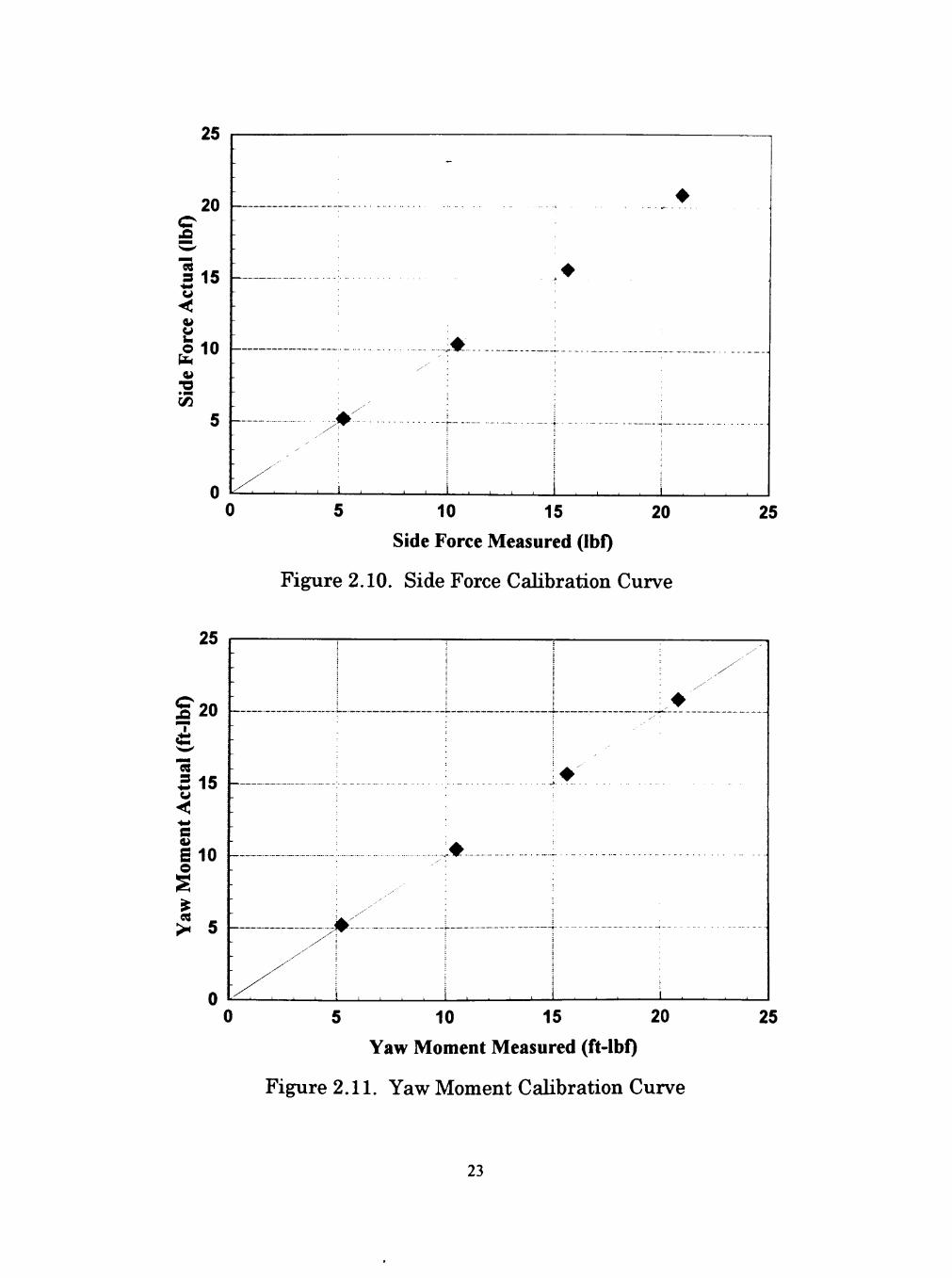
The resulting maximum errors for the caUbration are shown in Table 2.2.
Table 2.2. CaUbration Maximum Percent Error Results
Component
Lift
Drag
Side Force
Yaw Moment
RoU Moment
Pitch Moment
Maximum Percent Error
0.572
1.165
0.439
0.514
7.060
11.208
Maximum Percent Error
ofTop75%ofLoads
0.137
0.122
0.438
0.141
2.318
1.653
The maximum errors occurred at the lower range of the caUbration where
error is not as sigmficant because the objectiye is to determine the maximum
wind loadings. The caUbration coefficient matrix is shown in equation 2.2.
^ i j =
-0.068623
-0.000043
0.000567
0.000065
-0.001578
-0.001385
0.002713
-0.097639
-0.003474
-0.003210
0.000540
0.772837
-0.000941
0.004481
-0.098628
-0.003098
0.768802
-0.048991
-0.003027 0.000901
-0.001394
0.145119
-0.002156
-0.014981
-0.000064 -0.001540
-0.001236
-0.003456
-0.517809
0.016475
0.001724 0.003156
0.002542
0.004262
-0.020676
-0.602642
(2.2)
As can be seen in equation 2.2, the coefficients for Uft, drag, side force, and
yaw moment channels are diagonaUy dominant but the coefficients for roU
and pitch moment are not. A reyiew of the bridge configuration for the load
25

ceU indicated that a significant degree of cross-coupling could be expected for
side force on roU and drag on pitch. This result can be seen in yalues for asa,
ass and a62, ase.
Model
For this experiment, a one tenth scale model was buUt by Cummins
Power Generation to be tested in the tow tank. The model is shown in Figure
2.14. This figure also includes the support pipe and elbow that connects the
model to the load ceU. A fiberglass surface was used to simulate the
paraboUc reflecting surface of the concentrator. A steel rod space frame
backed the fiberglass surface for rigidity and repUcates the actual
concentrator support structure. The concentrator model was attached to a
support pole at a connection which aUows for pitch adjustments up to 360
degrees at increments of 15 degrees. The purpose of the support pole was to
connect the model to the load ceU which would place the center point of the
model at a depth of 5 feet. It is important to note that the model was
attached to the support pole upside down for ease of pitch adjustments. The
flange where the support pole attaches to the load ceU aUows for yaw
adjustments of up to 360 degrees. Figures 2.15 and 2.16 show a schematic of
the model, load ceU, support pole, and the direction of positiye forces and
moments.
Measurement of Forces and Moments
A combination of the aboye systems and setups is necessary for the
measurement the simulated wind forces and moments induced on the
concentrator model. The model and support pole are connected to the load
26

Figure 2.14. One-tenth Scale Model of Solar Concentrator
27
Side Force
Mount ing B r a c k e t
L i f t
i >Yaw
Pole-
I n v e r t e d C o n c e n t r a t o r ( no t ch up")
Drag
Roil
Pi tch
Load Ceil
78.5
Point o f C a l i b r a t i o n
No te : All dimensions a r e in inches, N o t t o sca le ,
Figure 2.15. Load CeU, Support Pipe, and Model Setup with Direction of Positiye Forces and
Moments (Drawn by RocheUe Pritchard)
28
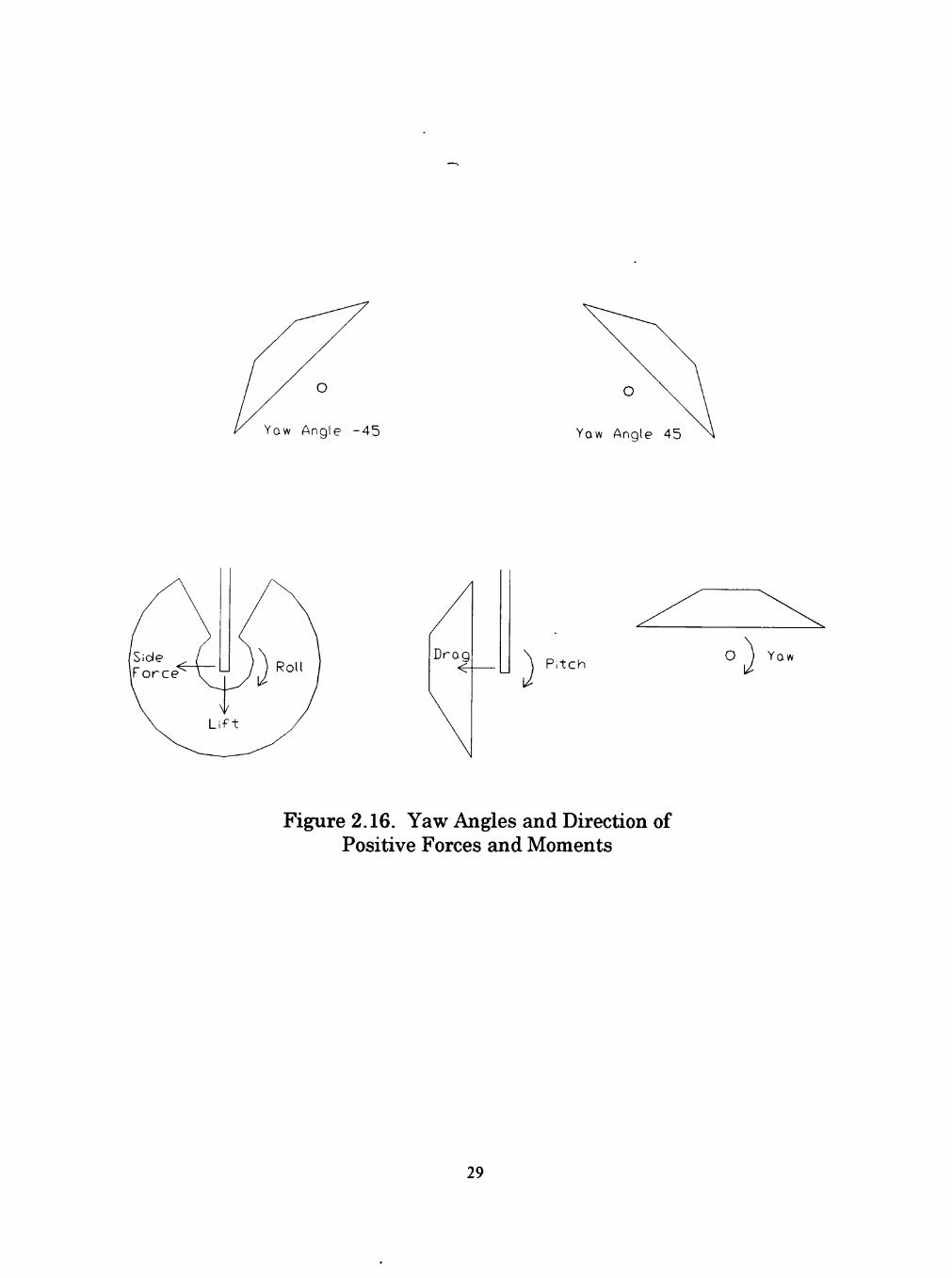
Yaw Angle - 4 5 Yaw Angle 45
P i t ch O Yaw
Figure 2.16. Yaw Angles and Direction of Positiye Forces and Moments
29

ceU which is attached to the front center of the bridge. After the cables are
connected to the data acquisition system, testing can begin. A program
written by Dr. Oler is used to control the data acquisition and measurement
of the forces and moments. The program sayes the model type, date of run,
yelocity, pitch and yaw angles, forces and moments, and yoltage differences.
Before data is taken, the bridges of each channel of the strain gage ampUfier
must be balanced because the initial output is caused by the static weight of
the model and support pole. After the bridges are balanced, the program
begins the data acquisition process with the recording of the zeroes of each
channel. Zeroes are taken at 100 Hz for ten seconds. The program then
requires that the desired run speed be entered. The run begins by
accelerating up to the desired speed in a two second time span. To insure
that the data is taken at the desired speed, once on speed, the bridge trayels
an additional 20 feet (5.72 model diameters) before beginning data
acquisition. Data is now recorded for the desired run speed and
configuration. Two data sampling frequencies were used to eyaluate the
effect of fluid induced oscUlations on the model. Frequencies of 100 Hz for
1000 data points and 150 Hz for 900 data points were used and resulted in
no sigmficant differences between the two frequencies. Zero load yoltages
are subtracted from the ayerage of the data points resulting in the net
yoltage differences caused by the simulated wind loadings on the model. The
net yoltage differences were multipUed by the coefficient matrix to calculate
the resulting loads. Ten runs were made for each configuration and then
ayeraged. It is important to note that these ayeraged loads include the loads
due to both the model and support pole. To obtain the load due to the
support pole solely, the process was repeated at each configuration of the
support pole alone. The ayeraged data of the support pole alone were
30

subtracted from the ayeraged data due to the support pole and model to
result in the net load caused by just the model. This data was used in the
calculations of the coefficients.
The speed of the tests were Umited by the capacity of the load ceU. It
was determined that the maximum safe test yelocity was 2.5 ft/s. This
resulted in a Re5molds number of approximately 808,000. This Re5niolds
number is greater than the Reynolds number that recommended by Roschke.
31

CHAPTER III
EXPERIMENTAL RESULTS AND DISCUSSION
The objectiye of the test program was to determine the maximum wind
loadings on the solar concentrator. To accompUsh this objectiye, a test
program was conducted using the Texas Tech tow tank. It was decided that
the tests should be done at pitch angles of 0, 30, 60, and 90 degrees and yaw
angles of 0, ±15, ±30, and ±45 degrees. Testing of the support pole with the
model was done first to confirm the maximum load estimates that were
assumed in the caUbration. The results showed that the loads measured
whUe testing feU within the caUbration range that was used. To find the
load that was induced by only the model, runs were made of only the support
pole. The model loads were found by subtracting the loads of the support
pole from the measured loads of the support pole and the model. The net
loads for the model were then conyerted into their nondimensional
counterparts. The nondimensional coefficients were plotted to eyaluate the
load characteristics as a function of pitch and yaw angles. Figures 3.1
through 3.6 show these results.
As can be seen from Figure 3.1, the Uft coefficients are symmetrical for
positiye and negatiye yaw angles. For pitching angles of 0 and 90 degrees,
the lift coefficient is relatiyely smaU. The minimum lift occurs at a 90degree
pitch angle which corresponds to a position with a minimum lift area
(maximum drag area). Lift is also smaU for a 0 degree pitch angle because
this position is the stow position or position of minimum loads. Lift increases
at a 30 and 60 degree pitch angles because as the pitch angle increases in the
30 to 60 degree range the area aboye and below the center of pressure
becomes unequal. This causes a pressure (force) difference causing a
32

I -0.3 S-0.4
U-0.5
'T 0 deg. Pitch 30 deg. Pitch 60 deg. Pitch 90 deg. Pitch
h -f—
-15 0 15 Yaw Angle (deg)
Figure 3.1. Lift Coefficients for Varying Yaw Angles
45
-15 0 15 Yaw Angle (deg)
Figure 3.2. Drag Coefficients for Varying Yaw Angles
33
-15 0 15 Yaw Angle (deg)
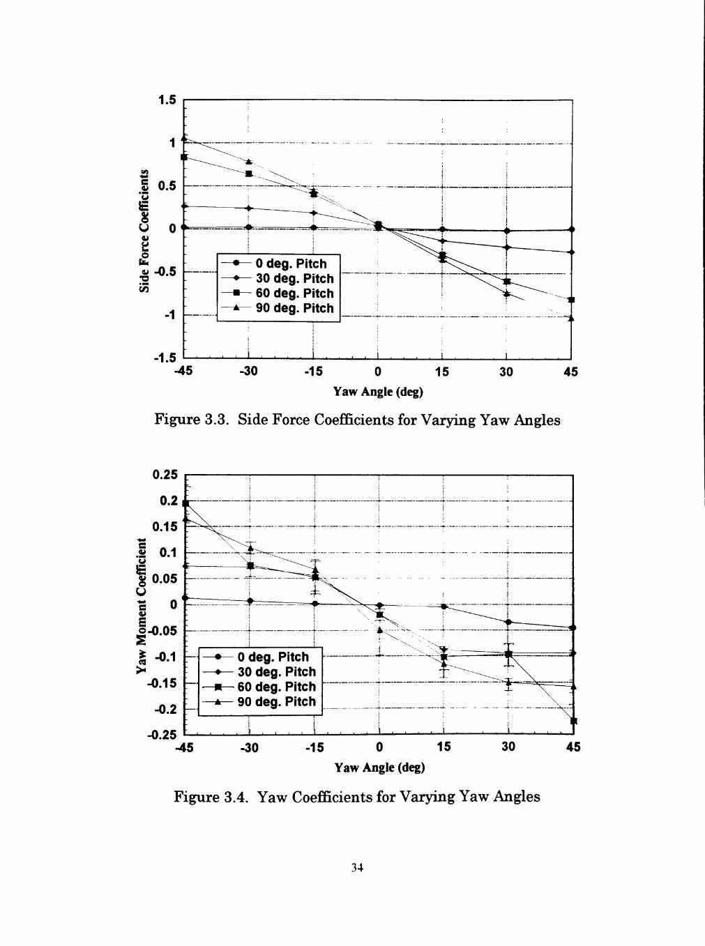
Figure 3.3. Side Force Coefficients for Varying Yaw Angles
-15 0 15 Yaw Angle (deg)
Figure 3.4. Yaw Coefficients for Varying Yaw Angles
34
I 0.4 £ ^ 0.2 ••* c E 0 o
-0.4
-0.6
- K ^
\ \
^— 0 deg. Pitch -•— 30 deg. Pitch ^— 60 deg. Pitch ^— 90 deg. Pitch
' I I I I I I
-45 -30 -15 15 30 45
Yaw Angle (deg)
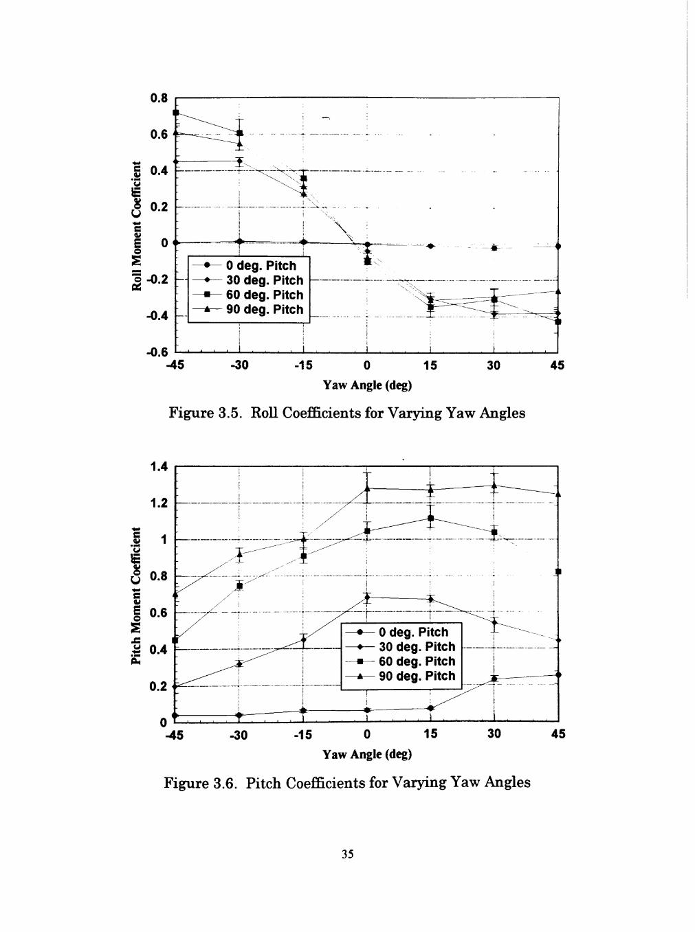
Figure 3.5. RoU Coefficients for Varying Yaw Angles
s .Si 'S €
• * *
e B o 0 deg. Pitch
*— 30 deg. Pitch 60 deg. Pitch
A— 90 deg. Pitch
_L. I I i
-45 -30 •15 0 15
Yaw Angle (deg)
30 45
Figure 3.6. Pitch Coefficients for Varying Yaw Angles
35

negatiye Uft coefficient. The maximum Uft coefficient of -0.92 occurs at a yaw
angle of 0 degrees and 30 degrees pitch. Maximum lift coefficients at each
pitch angle occurred at a yaw angle of 0 degrees. This is apparently due to
the notch in the model which is shown in Figure 2.16. The yariances shown
in the figure shows that data runs were repeatable.
The drag coefficient results are shown in Figure 3.2. The figure shows
that the drag steadUy increases as the pitching angle increases and as the
yaw angle approaches 0 degrees. The trend results from the fact that the
frontal area increases as the pitching angle increases and the yaw angle
approaches 0 degrees, as shown in Figure 2.16. It is logical then that the
point of maximum drag should occur at a 0 degree yaw angle and 90 degrees
of pitch and a minimum drag occurs at a pitch angle of 0 degrees. As the
figure shows, the corresponding maximum drag coefficient of 1.42 occurs at
this point. In addition, the figure shows that whUe the yariation in drag
coefficient data is smaU at 0 and 30 degree pitching angles, the yariance
increases for 60 and 90 degree pitching angles. But since the trends and
symmetry are in agreement with theory and the yariances are relatiyely
smaU, the drag results should be suitable to proyide an estimate for wind
loadings with a low uncertainty.
Side force coefficient results for yarying yaw angles are shown in
Figure 3.3. These results show that the side force loads are symmetrical for
both positiye and negatiye yaw angles. As explained aboye, the opposite
signs for the side force are a result of the center of pressure rotating from one
side of the caUbration point to the other. The side force yariances in the data
are also smaU showing that the data was consistent for multiple runs. A
minimum side force occurs at a yaw angle of 0 degrees for aU the pitch angles
because the center of pressure occurs along the axis of the caUbration point
36
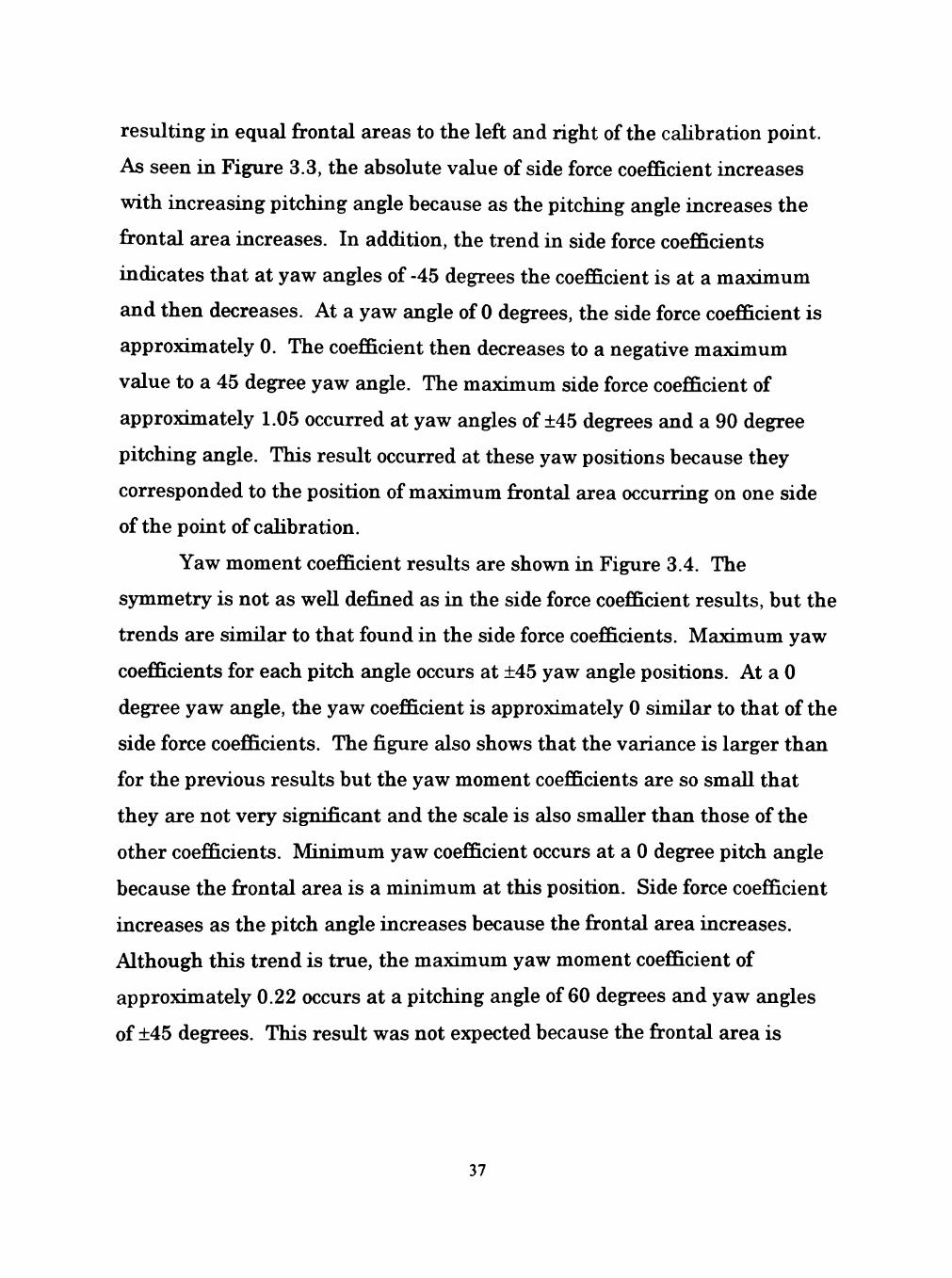
resulting in equal frontal areas to the left and right of the caUbration point.
As seen in Figure 3.3, the absolute yalue of side force coefficient increases
with increasing pitching angle because as the pitching angle increases the
frontal area increases. In addition, the trend in side force coefficients
indicates that at yaw angles of -45 degrees the coefficient is at a maximum
and then decreases. At a yaw angle of 0 degrees, the side force coefficient is
approximately 0. The coefficient then decreases to a negatiye maximum
yalue to a 45 degree yaw angle. The maximum side force coefficient of
approximately 1.05 occurred at yaw angles of ±45 degrees and a 90 degree
pitching angle. This result occurred at these yaw positions because they
corresponded to the position of maximum frontal area occurring on one side
of the point of caUbration.
Yaw moment coefficient results are shown in Figure 3.4. The
S5rmmetry is not as weU defined as in the side force coefficient results, but the
trends are similar to that found in the side force coefficients. Maximum yaw
coefficients for each pitch angle occurs at ±45 yaw angle positions. At a 0
degree yaw angle, the yaw coefficient is approximately 0 simUar to that of the
side force coefficients. The figure also shows that the yariance is larger than
for the preyious results but the yaw moment coefficients are so smaU that
they are not yery significant and the scale is also smaUer than those of the
other coefficients. Minimum yaw coefficient occurs at a 0 degree pitch angle
because the frontal area is a minimum at this position. Side force coefficient
increases as the pitch angle increases because the frontal area increases.
Although this trend is true, the maximum yaw moment coefficient of
approximately 0.22 occurs at a pitching angle of 60 degrees and yaw angles
of ±45 degrees. This result was not expected because the frontal area is
37

maximum at 90 degrees pitch. The effect of the notch and/or the indicated
data yariation may contribute to this result.
Figure 3.5 shows the results of the roU moment coefficients for yarying
yaw angles. Although the figure appears to be symmetrical, the numbers do
not coincide for both positiye and negatiye yaw angles. The trends are
consistent with expectations from -45 to 15 degree yaw angles. Howeyer, at
30 degree yaw angle, the absolute yalue of the 60 and 90 degree pitch angle
roU coefficient data are lower than the 30 degree pitch angle roU coefficients.
If the data was extrapolated from the 15 degree yaw angle to the 45 degree
yaw angle, it appears that the data would correspond to their negatiye yaw
angle positions. The difference of the positiye and negatiye yaw angle roU
coefficients could be caused by seyeral factors including caUbration errors
and the effects of the support pole on the model. Howeyer, the yariances in
the roU coefficients indicate that the runs were repeatable for at least 10 runs
for each point and that this result might be inherent in the solar concentrator
model. The maximum roU moment coefficient occurred at a yaw angle of -45
degrees and a pitch angle of 90 degrees. This maximum yalue was
approximately 0.72.
The pitch moment coefficients are shown in Figure 3.6. As can be
seen, the figure does not appear symmetrical. The expected trend is similar
to that found in the drag coefficients in Figure 3.2. The minimums should
occur at the ±45 yaw angles and the coefficients should increase to a
maximum at a 0 degree yaw angle. Also, the pitch coefficients should
increase as the pitch angle increases. Signs of these trends are eyident in
Figure 3.6. The pitch coefficient does increase as the pitch angle increases
and is a maximum at a 0 degree yaw angle. Howeyer, the yalues at positiye
and corresponding negatiye yaw angles are not equal. Part of this problem
38

could be accounted for as part of a continual problem found in the caUbration
of the pitch moment. The errors in the caUbration could not be reduced in
the pitch moment. The errors are beUeyed to be caused from caUbrating
about a point which is approximately 6.5 ft below the load ceU. The total
pitch moment, as seen from the load ceU, is the appUed moment from the
caUbration and a contributing moment caused by the drag force being appUed
with a 6.5 ft moment arm. Eyen though the trends do not correspond with
expected trends, the maximum pitch moment coefficient seen in Figure 3.6 is
approximately 1.3 at a 90 degree pitch and 0 degree yaw angle. Variances in
the pitch coefficients are significant for the 90 degree pitch angle position.
This position corresponds to the location of the maximum pitch coefficient.
In an effort to find other possible solutions in the errors of sjnnmetry
found in the roU and pitch results, fiirther testing of the load ceU was done.
There could be seyeral possible reasons for this phenomena, such as, there
could be a problem in the caUbration, the model was not buUt symmetricaUy,
or a problem in the design of the load ceU. To rule out the design of the load
ceU, further tests were done. These tests were done with the load ceU in the
caUbration position. Known weights were appUed to determine how, for
example, the roU output yaries as the drag is increased. Initial results haye
shown that the Uft, drag, side force, and the yaw appear to be reasonably
accurate except at loads under 10 pounds. The roU and pitch results showed
that the load ceU was measuring loads which were larger than appUed.
Again this could be from the results of a bad caUbration or from a problem
with the design of the load ceU. The requirement in this test program to
caUbrate at 6.5 ft below the load ceU tended to increase the uncertainty in the
calculated and measured loads. One of the other efforts that was performed
on the load ceU was rotating the load ceU and applying a load. This effort
39

was performed to confirm that the load ceU was aUgned correctly. The
results of this testing showed that the load ceU was aUgned symmetricaUy.
In summary, the trends of affects of yaw and pitch angles were
generaUy consistent with physical expectations. Most components exhibit
symmetrical load characteristics. The Uft, drag, side force, and yaw figures
show that the coefficients are symmetrical with only minor discrepancies.
Howeyer, for the roU and pitch components, the discrepancies became
significant. One significant trend in the symmetry of the Uft, drag, and pitch
moment coefficients is that the coefficients are approximately the same for
both positiye and negatiye yaw angles. This is due to the geometry of the
model and the direction of the forces and moments which can be seen in
Figure 2.16. In the same manner, the side force, yaw moment, and roU
moment coefficients are opposite in sign for positiye and negatiye yaw angles.
40

CHAPTER IV
CONCLUSIONS AND RECOMMENDATIONS
The objectiye of this research project was to determine the wind
loadings on a notched paraboUc solar concentrator. The results from Texas
Tech's tow tank testing of the one tenth scale model were put into
nondimensional force and moment coefficients. Since the nondimensional
coefficients are yaUd for both the model and the actual solar concentrator
prototype, they are the major results of the project. The maximum
coefficients are shown in Table 4.1.
Table 4.1. Maximum Nondimensional Coefficient Results
Component
Lift
Drag
Side Force
Yaw Moment
RoU Moment
Pitch Moment
Coefficient
-0.92
1.42
1.05
-0.23
0.72
1.28
Based on the aboye resiUts, the structural design of the solar concentrator
support structure should use these results for maximum load estimates.
Howeyer, as seen preyiously, the roU and pitch moment coefficients haye
errors in the figures because S5anmetry is not present from negatiye to
positiye yaw angles. These yalues could be only used as a starting estimate
for the beginning stages of the structural design.
41

There are stUl seyeral things that could be done in the future which
would make the work more conclusiye. Some of the things that could be done
include:
• Determine the problem with the roU and pitch measuring false loads.
• If the problem is with the design of the load ceU, then the load ceU must
be redesigned or purchase a new load ceU.
• Retesting of the model in the tow tank for the configurations tested for
this project and for different configurations such as the model being
rotated on one side (the y-notch on one side).
• Flow yisualization can also be performed on the model.
• Computational fluid dynamics program inyestigation of the model.
42
REFERENCES
Imadojemu, H. E., "Literature Suryey of Concentrating Solar CoUectors," Solar Enedneering. Vol. 1, pp. 719-730, 1995.
Murphy, L.M., "Wind Loading on Tracking and Field Mounted Solar CoUectors," Proc. ASME Solar Energy Diyision. Solar Engineering -1981. edited by Reid, R.L., Murphy, L.M., and Ward, D.S., pp. 719-727, April 1981.
Roschke, E. J., Wind Loading on Solar Concentrators: Some General Considerations. U.S. Dept. of Energy DOE/JPL-1060-66, May 1, 1984.
Stine, W. B., "An International Suryey of paraboUc Dish/StirUng Engine Electrical Power Generation Technology," Solar Engineering 1993. pp. 421-427, 1993.
Stine, W. B. and R. B. Diyer, A Compendium of Solar Dish/StirUng Technology. SAND93-7026 UC-236, Albuquerque, NM: Sandia National Laboratories, January 1994.
Wyatt, T. A., "The Aerodynamics of ShaUow Paraboloid Antennas," Annals. New York Academy of Sciences. Vol. 116, pp. 223-238, 1964.
43

APPENDIX A
CALIBRATION DATA
44
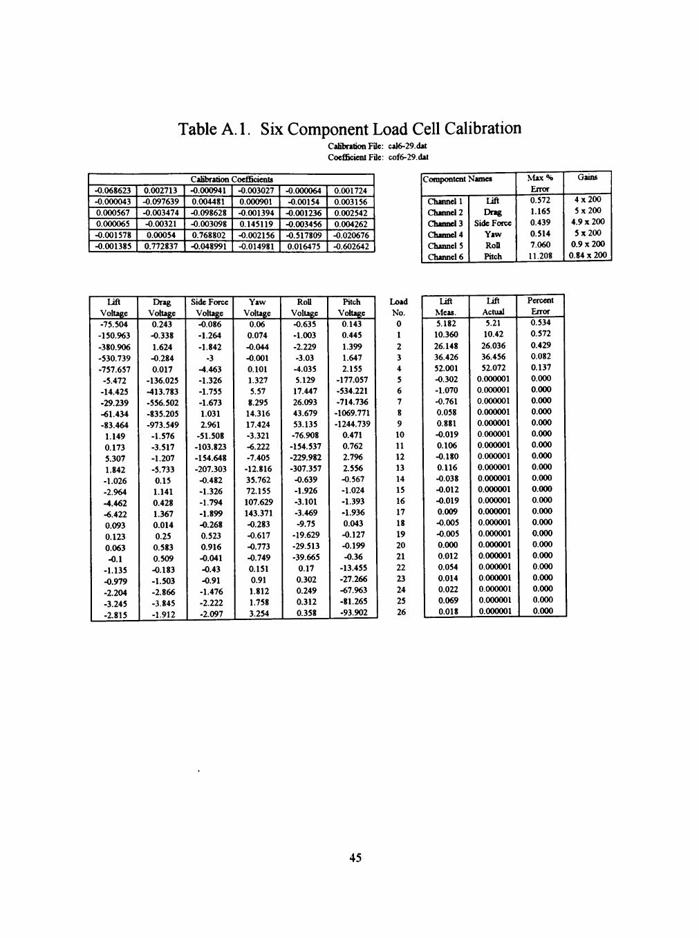
Table A. 1. Six Component Load CeU CaUbration CaUbntkm Fac: cal6-29.dat Coefficient File: cof6-29.dat
Calibration CoefBcients -0.068623 -0.000043 0.000567 0.000065 -0.001578 -0.001385
0.002713 -0.097639 -0.003474 -0.00321 0.00054 0.772837
-0.000941 0.004481 -0.098628 -0.003098 0.768802 •0.048991
-0.003027 0.000901 -0.001394 0.145119 -0.002156 -0.014981
-0.000064 -0.00154 -0.001236 -0.003456 •0.517809 0.016475
0.001724 0.003156 0.002542 0.004262 -0.020676 -0.602642
Compontent
Channel 1 Channel 2 Channel3 Channet4 Channel 5 Channel 6
>iamea
Lift Drag
Side Force Yaw Ron Pitch
Max% Error 0.572 1.165 0.439 0.514 7.060 11.208
Gains
4x200 5x200
4.9 X 200 5x200
0.9 x 200 0.84 X 200
Lift Voltage -75.504 -150.963 -380.906 -530.739 -757.657 -5.472 -14.425 -29.239 -61.434 -83.464
1.149 0.173 5.307 1.842 -1.026 -2.964 •4.462 -6.422 0.093 0.123 0.063 -0.1
-1.135 -0.979 -2.204 -3.245 -2.815
Drag Voltage 0.243 -0.338 1.624 -0.284 0.017
-136.025 •413.783 -556.502 -835.205 -973.549
-1.576 -3.517 •1.207 •5.733 0.15 1.141 0.428 1.367 0.014 0.25 0.583 0.509 •0.183 •1.503 -2.866 •3.845 •1.912
Side Force Voltage •0.086 •1.264 •1.842
•3 •4.463 •1.326 •1.755 •1.673 1.031 2.961
-51.508 •103.823 •154.648 •207.303 •0.482 •1.326 -1.794 •1.899 •0.268 0.523 0.916 •0.041 -0.43 -0.91 •1.476 •2.222 -2.097
Yaw Voltage
0.06 0.074 -0.044 -0.001 0.101 1.327 5.57 8.295 14.316 17.424 -3.321 -6.222 -7.405 •12.816 35.762 72.155 107.629 143.371 -0.283 •0.617 •0.773 -0.749 0.151 0.91 1.812 1.758 3.254
RoU Voltage -0.635 -1.003 -2.229 -3.03 -4.035 5.129 17.447 26.093 43.679 53.135 -76.908 -154.537 -229.982 -307.357 -0.639 -1.926 -3.101 -3.469 -9.75
-19.629 -29.513 -39.665
0.17 0.302 0.249 0.312 0.358
Pitch Vohage 0.143 0.445 1.399 1.647 2.155
-177.057 -534.221 -714.736 -1069.771 -1244.739
0.471 0.762 2.796 2.556 -0.567 -1.024 -1.393 -1.936 0.043 -0.127 •0.199 -0.36
-13.455 -27.266 -67.963 -81.265 -93.902
Load No. 0 1 2 3 4 5 6 7 8 9 10 11 12 13 14 15 16 17 18 19 20 21 22 23 24 25 26
Lift Meas. 5.182 10.360 26.148 36.426 52.001 -0.302 -1.070 -0.761 0.058 0.881 -0.019 0.106 -0.180 0.116 -0.038 -0.012 •0.019 0.009 •0.005 •0.005 0.000 0.012 0.054 0.014 0.022 0.069 0.018
Lift Actual 5.21 10.42
26.036 36.456 52.072
0.000001 0.000001 0.000001 0.000001 0.000001 0.000001 0.000001 0.000001 0.000001 0.000001 0.000001 0.000001 0.000001 0.000001 0.000001 0.000001 0.000001 0.000001 0.000001 0.000001 0.000001 0.000001
Percent Error 0.534 0.572 0.429 0.082 0.137 0.000 0.000 0.000 0.000 0.000 0.000 0.000 0.000 0.000 0.000 0.000 0.000 0.000 0.000 0.000 0.000 0.000 0.000 0.000 0.000 0.000 0.000
45
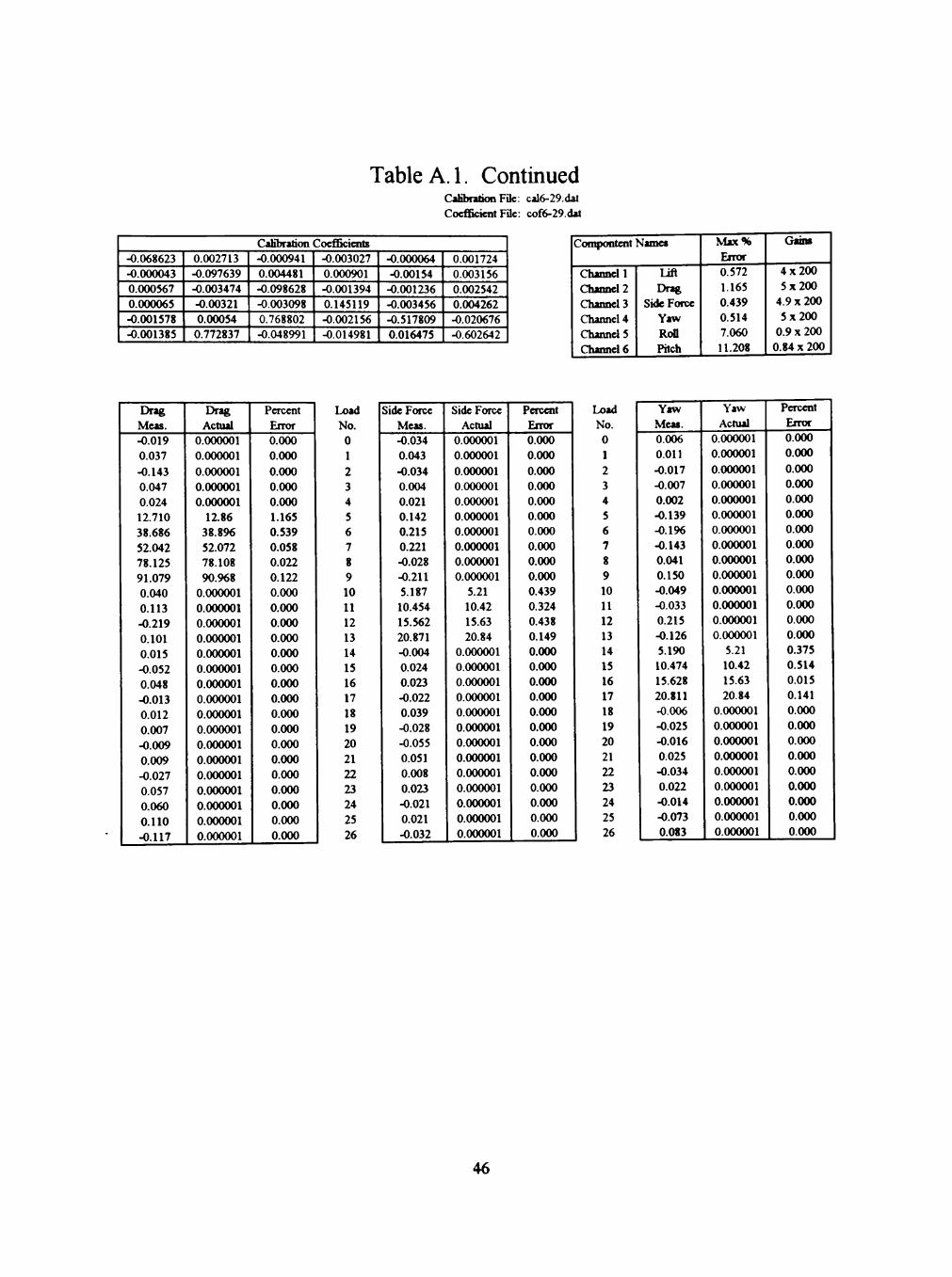
Table A. 1. Continued Calibration File: cal6-29.dat CoefiBcient Ffle: cof6-29.dat
Calibration CoefiBcients •0.068623 -O.000043 0.000567 0.000065 •0.001578 -0.001385
0.002713 •0.097639 -0.003474 -0.00321 0.00054
0.772837
-0.000941 0.004481 -0.098628 -0.003098 0.768802 -0.048991
-0.003027 0.000901 -0.001394 0.145119 -0.002156 -0.014981
-0.000064 -0.00154
-0.001236 -0.003456 -0.517809 0.016475
0.001724 0.003156 0.002542 0.004262 -0.020676 -0.602642
Compontent
Channel 1 Channel 2 Channel 3 Channel 4 Channel 5 Channel 6
Names
Lift Drag
Side Force Yaw Ron Pitch
Max% Enor 0.572 1.165 0.439 0.514 7.060 11.208
Gains
4 x 2 0 0 5 x 2 0 0
4.9 X 200 5 x 2 0 0
0.9 X 200 0.84 X 200
Drag Meas. -0.019 0.037 -0.143 0.047 0.024 12.710 38.686 52.042 78.125 91.079 0.040 0.113 -0.219 0.101 0.015 -0.052 0.048 -0.013 0.012 0.007 -0.009 0.009 -0.027 0.057 0.060 0.110 -0.117
Drag Actual
0.000001 0.000001 0.000001 0.000001 0.000001
12.86 38.896 52.072 78.108 90.968
0.000001 0.000001 0.000001 0.000001 0.000001 0.000001 0.000001 0.000001 0.000001 0.000001 0.000001 0.000001 0.000001 0.000001 0.000001 0.000001 0.000001
Percent Error 0.000 0.000 0.000 0.000 0.000 1.165 0.539 0.058 0.022 0.122 0.000 0.000 0.000 0.000 0.000 0.000 0.000 0.000 0.000 0.000 0.000 0.000 0.000 0.000 0.000 0.000 0.000
Load No.
0 1 2 3 4 5 6 7 8 9 10 11 12 13 14 15 16 17 18 19 20 21 22 23 24 25 26
Side Force Meas. -0.034 0.043 •0.034 0.004 0.021 0.142 0.215 0.221 -0.028 -0.211 5.187 10.454 15.562 20.871 -0.004 0.024 0.023 -0.022 0.039 -0.028 -0.055 0.051 0.008 0.023 -0.021 0.021 •0.032
Side Force Actual
0.000001 0.000001 0.000001 0.000001 0.000001 0.000001 0.000001 0.000001 0.000001 0.000001
5.21 10.42 15.63 20.84
0.000001 0.000001 0.000001 0.000001 0.000001 0.000001 0.000001 0.000001 0.000001 0.000001 0.000001 0.000001 0.000001
Percent Error 0.000 0.000 0.000 0.000 0.000 0.000 0.000 0.000 0.000 0.000 0.439 0.324 0.438 0.149 0.000 0.000 0.000 0.000 0.000 0.000 0.000 0.000 0.000 0.000 0.000 0.000 0.000
Load No.
0 1 2 3 4 5 6 7 8 9 10 11 12 13 14 15 16 17 18 19 20 21 22 23 24 25 26
Yaw Meas. 0.006 0.011 -0.017 -0.007 0.002 •0.139 -0.196 •0.143 0.041 0.150 •0.049 -O.033 0.215 -0.126 5.190 10.474 15.628 20.811 -0.006 -0.025 -0.016 0.025 -0.034 0.022 -0.014 -0.073 0.083
Yaw Actual
0.000001 0.000001 0.000001 0.000001 0.000001 0.000001 0.000001 0.000001 0.000001 0.000001 0.000001 0.000001 0.000001 0.000001
5.21 10.42 15.63 20.84
0.000001 0.000001 0.000001 0.000001 0.000001 0.000001 0.000001 0.000001 0.000001
Percent Error 0.000 0.000 0.000 0.000 0.000 0.000 0.000 0.000 0.000 0.000 0.000 0.000 0.000 0.000 0.375 0.514 0.015 0.141 0.000 0.000 0.000 0.000 0.000 0.000 0.000 0.000 0.000
46

Table A. 1. Continued Calibration File: cal6-29.dat Coefficient File: cof6-29.dat
Calibration Coefficients -0.068623 -0.000043 0.000567 0.000065 -0.001578 -0.001385
0.002713 -0.097639 •0.003474 •0.00321 0.00054
0.772837
•0.000941 0.004481 •0.098628 •0.003098 0.768802 -0.048991
•0.003027 0.000901 -0.001394 0.145119 -0.002156 •0.014981
-0.000064 -0.00154
-0.001236 -0.003456 -0.517809 0.016475
0.001724 0.003156 0.002542 0.004262 -0.020676 -0.602642
Compontent
Channel 1 Channel 2 Channel 3 Channel 4 Channel 5 Channel 6
Names
Lift Drag
Side Force Yaw
Ron Pitch
Max% Error 0.572 1.165 0.439 0.514 7.060 11.208
Gains
4 x 2 0 0 5 x 2 0 0
4 .9x200 5 x 2 0 0
0.9 x 200 0.84 X 200
RoU Meas. 0.379 -0.224 0.311 0.066 -0.191 -0.082 0.449 -0.292 -0.091 0.067 0.219 0.197 0.142 -0.254 -0.103 -0.151 0.031 0.078 4.842 10.570 15.992 20.517 •0.139 •0.293 0.140 •0.190 0.140
RoU Actual
0.000001 0.000001 0.000001 0.000001 0.000001 0.000001 0.000001 0.000001 0.000001 0.000001 0.000001 0.000001 0.000001 0.000001 0.000001 0.000001 0.000001 0.000001
5.21 10.42 15.63 20.84
0.000001 0.000001 0.000001 0.000001 0.000001
Percent Error 0.000 0.000 0.000 0.000 0.000 0.000 0.000 0.000 0.000 0.000 0.000 0.000 0.000 0.000 0.000 0.000 0.000 0.000 7.060 1.440 2.318 1.551 0.000 0.000 0.000 0.000 0.000
Load No. 0 1 2 3 4 5 6 7 8 9 10 11 12 13 14 15 16 17 18 19 20 21 22 23 24 25 26
Pitch Meas. 0.199 •0.276 0.994 •0.380 -0.086 1.714 2.467 1.073 -0.249 -1.678 -0.197 -0.544 1.273 -0.689 -0.064 0.455 -0.399 0.120 -0.158 -0.070 0.051 -0.030 7.990 15.307 38.795 46.094 55.175
Pitch Actual
0.000001 0.000001 0.000001 0.000001 0.000001 0.000001 0.000001 0.000001 0.000001 0.000001 0.000001 0.000001 0.000001 0.000001 0.000001 0.000001 0.000001 0.000001 0.000001 0.000001 0.000001 0.000001
7.185 15.63
39.054 46.869 54.684
Percent Error 0.000 0.000 0.000 0.000 0.000 0.000 0.000 0.000 0.000 0.000 0.000 0.000 0.000 0.000 0.000 0.000 0.000 0.000 0.000 0.000 0.000 0.000 11.208 2.064 0.664 1.653 0.899
47
APPENDIX B
SUPPORT PIPE DATA
48

t l O
o
^^ i i o
CU
CD
CO
(2
3.50
j ^ « •
?
22/9
^
O
9.62
A
ref-
SJV
P
3
•3 •8 2
1.93
8
1
Poi
oiit
y-
m Q
o
a
3 « o> »• <N fS .^ v^ • 3 •« u 8
1^ I i S 33
II u u
a: S o
8 m o 5
»: S o
s J "3
" 1 jg
J* <-. ^ 8
^ ^
2
Dra
g
94x2
00
•«>
s - «"3
-J ;s Cl
* 1 § M
« o
Loa
d
<« S
. .o J .
5 a.
RM
'(
*r?
;- £ V-
^
82
s ^ u
? tr. - J
« >
« '9i B
hing
•R M
"O O
i n
s? 0^
o
tv i n
o
in
•-J o
§ tM
e
1 •B. M
•o
s
s
(
1 o
§ Til
»-«
» fM O
M <s
!3 as
1 •B. ae •a e
3 ^
% r-«
1 - t
1 - t
f^
O i - t
'^
g •qi l - H
?1 00 d
S (N
« -a b
chin
g
-EL as
t l
e
2 ©> M
(N
S a
'?
m i - »
s •
^ CM
OB
o l«
0 u
u
00 7
1 ^
s s ;£ s in ^ in in o o ^ ^
• 1-1 t l fS
5 S S 3 d d e> d
o m » t CJ <3 •-' Q o o o S d ^ d ti
ts ^ » o o o o 8 d d d d
n * in m (M <N H
d d d o
S S S 8 o d d d
<= S 3 8
H
« ! l
C 3
- 5
^ 2 3 ^
8! A
S « ^ S " S S
2 !!5 8 ^
o S S 8
49
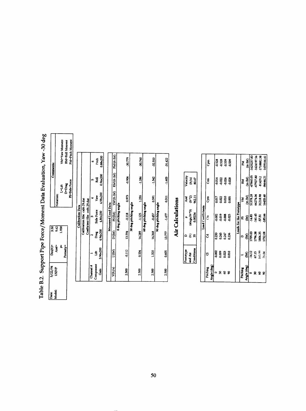
O en
I
o
>
«k
u
•Yaw
Mom
ent
-RoU
Mom
ent
Pitc
h M
omen
t
lis >• BS OL.
Not
atio
n: L
-Lif
t D
-Dra
g F
S-Sl
de F
orce
c s
S ^ rt
g ta
I =3 u
I i
.2 •«
* I 3
s t ^ NO
en
« 8
S „ « "2
5
•B. as
I =
-ab
s
as ai
s5
I S
•S "*
00 e o
u
I
00 _
5 S
fs (N in ft in in in in 9 9 9' 9
NO r4 so «o
5 § 8 S o* o* o c>
tv rsi o in
5 § S S o c> o c>
§ o oo in s i s d d d d
d d d d
o d
<= S S 8
s l
I
^S
i -
a 3? ? 5 a I i I m •« 2 9 (N (N r - m so so tN. sO
S 8 ^ S
5 ^ « s
R Ji :S ." Cl 2 <N ^ in S c> •>
S CO m ao
. m (n q 2; *P ^ <N
8 R S R
2 - ? s =r 5S 2 s
° S S 8
50

to -o ID rH
I
e o
IS >
c a; s o
u o
p a; OH
O
a. 3
CD
CO
s2
3.50
J.
22/9
4
~«.
« (3
9.62
A
ref-
SJV
P
D
•3 ^ S
1.93
8
A.
Por
otit
y-
Q e
ilib
nti
o
(;
9.da
t 9.
dat
<N (N vtb v ^ •3 Tl u 8
tion
file
: le
nt f
ile:
a M
alib
oe
ff
u u
^ 8 >e ^ 2
£ S o
8 in o 5
• * OS o
8
4 Y
aw
4.98
x2
* m
a 8
3 Si
de F
o 4.
86x2
^8
Cha
nnel
* 1
2 C
ompo
nent
Lt
ft D
raj
Gai
n 3.
96x2
00
4.94
x2
Dat
a:
Loa
d
1 (ft
s
c-
-lb
•t;
S a.
9
s 5
(ft-1
H
^
ffi
b
2 ZJ
>
« •all
s
hing
pi
U
as •9 e
Ov
CN
-33
fi o
705
o
498
o
924
( S
.169
o
500
H
angl
e ch
ing
pit
as TJ
s
^ VO
-32
t?
886
o
370
T
958
370
o
500
r4
angl
e ch
ing
pit
as •o e VO
* i n
^
i n i n
o
544
o
101
t - l
095
•fli
714
o
500
CM
angl
e ch
ing
pit
as at Tl
O 9v
i n
»
i n
o • ^
301
120
r H
235
m
380
o
500
(N
to
o
in in in d d 9
§ » o 8 o
d o d
rM in ch in o o 8 8
§ 11 o> » 8 S S
o d ^ ^
a o ^ tx tM CM 9
d d d d
iis o a d d
<= S S 8
s l
EG £ •
_ 2
| 4
2 ^ 8 8 o^ ed so (*5
a 2 £ g ^ S i n I i
^
2 2 9 Ji
R S fe « o • • <s
^ d I
tc {; 8 ^
?l « f: 8 ?? S S 5j
° S S 8
51
Ol •a o as
>^
O
3
>
S <a
O c B o u o a;
1-1 o a. 3
CD
CO
:H i2
s m
J
Dm
(
in
1^
Q
so OS
^
P tn 3
•3 •B
s
00
1 1
Poro
*
m
Q g •r
a
9.da
t 9.
dat
(N CN v ^ ^
•a "R
fUe:
c
file:
c
II S 33
alib
oe
ft
u o
^ 8 - "S 2 £ S
o
8
oi S o
8 s "a "C 00 >* OL
«
3 eFor
c 36
x20C
S ^
„„8
Cha
nnel
#1
2 C
ompo
nent
Li
ft D
ra
Gai
n 3.
96x2
00
4.94
x2
•B. as « •o o
•a, e
S
-ak
s S as
d o
I
ity
H •3 >
Are
f
a.
O
S.
oty
Prot
^ «
CM" <
m < LC
9
-s
(ft)
A
il an
d
tx VO
^
62.1
1
OS
m
^ o
in m
i
ditl
C
on
(N 2| o* o in in in m 9 9 9 9
I o m «N
8 8 S d d d d
8 8 § § 9 o d d
r i VO r » o o o 8 d d d d
S ^ vO » «-• r- l f - l
r« CN CM <N
d d d d
8 § S 9 d d
<= S 3 8
r
s i
S 2
iC i
D S o
«6 . •S s
s q ffl a o ^ ^ ^
1^
CM v ^
9 -< flO o>
7 in
( ^ PsI
<0
•o 5 on "^
5 S Cl m
s S
S5J
R S
5 5 S R O 11 ao -~ CM Si
= ' 8 3 8
52
T3 in r-i S
;2 C o
> w S Hi Q c a; g o
^ ^ <u
o
C l .
o O H a 3
CD
iri CO Ci
s2
«i
u
Mom
ent
Mom
ent
Mom
ent
-Yaw
-R
oU
Pitc
h
lis >. otf o.
L-L
ift
D-D
rag
-Sid
e Fo
rce
Not
atio
n FS
3.50
D
m(f
t)-
22/9
4
• ^
D
9.62
A
ief-
SJV
P
3
"aJ •a a S
1.93
8
A.
Por
osit
y-
m
Q e o
-A • .& g (
- -4 <0
•o -o ^ OL CN rvl vi . i •3 -H u S
2 a
tion
lent
s u
Cal
ib
Coc
ft
^ 8 * ^ 2
s: S o
8 in o 5
« s o
^ 8 - i 3
^ OL
•" r^ O ^
Ci B. 3
2 3 («
Cha
nnel
*
1 2
Com
pone
nt
Lift
Dra
g G
ain
3.%
x200
4.
94x2
00
Q •a
ILoa
1 s s
. £ « s a.
% ai
^ Xi
a ^ ?
^ o e
&
5 o ZJ
>
^ 1 •i •a e
(N
^ CM
Ov m d
OO
m d
2
ov CM
1 o
§ CM
-ab
s as
chin
•B. as ai
•0 S
f; i - <
s
M
« O
s o 1-1
c>i
ci
tv CM in d
§ r l
ai -al)
s as
chin
•B. as
e VO
00
CN n
s » o
8 in d
in
g CO
i n
"
§ CM
e as
chin
•B. as a;
o ov
3 CM
^
in so (S *-H
s CM d
s CN
00 O
cn
g d
§ (N
CO
O
in so r ^ m in m m c> d d d
§ § § § d d d d
o o » 5 ^ ^ O w o o 8 o o o o o d d ^
8 i 8 i d d d d
CM o t^ o
a s a R d d d o
§ 8 . o o ° d d d
o S 3 8
sS
s £
D S
Ii " 5
8 R in (N
S 8
it '^i K
= ^ ^ 2
o S 3 8
53

bo
o CD
a o x:
"is >
S D c Ol
B o 01 u u O
o OH a 3
CD
sd
O)
Ii
u
-Yaw
Mom
ent
-RoU
Mom
ent
•Pitc
h M
omen
t
lis > " * • CL.
Not
atio
n: L
-Ltf
t D
-Dra
g F
S-«l
de F
orce
o
3.5
1
22/9
4
•*»*
o
CM
9.6
Are
f-SJ
VP
3
•3
•s s
00
1.93
A.
Por
osit
y-
II
^ 2
8 04 S
" I 2 'C 00 ' • Ov
8 o »• «
. '»'
8 ^ s "a
s
'&
Cvi
•B. as ai
• a e
? as
I s u
S?
3
? as
I •B. as
cvl
CA
o
ity
X •3 ^
1
a.
D
s.
oty
rot
CL.
^ K
(ft
CN <
•a - v . .
& 9
-3
(ft)
A
ir
and
t^ VO
OO
9621
00
234
o
in m
ons
diti
g u
I' (J
(J
00 00 »
S 5 i n i n
i n i n
d d d d
8 d
8 d
r- g 1-1 a o p O 8 d d d d
t ^ vO OL 11
8 S S S O ^ O Q
3 ^ tv CO i n i n • *
(N rs| fsj *N d d ^ d
^ d d
° S 3 8
S r
s
-.5
?q lq 8 * i n r^ so' 0-'
S i l l S 00 tv S
< ' • s » C S •"
s a Si R r ; tx' O s£ 00 m (-N (A
S ^ ?j 2
3 S Ji? 9 d i-J » t^ ^ vo Fv ^ Fs « 00 00
**; ^ " i ^
=: : S 8!
° S 3 8
54

T3
.o
>
3 <a D c
u
o
u
g 1 e g g H
s s s S a -g « Q i i
^ "i f l i s > . 06 Ol.
« b:
_ 60 O 5 g tt.
f 9 -S • D f g £ « o
2
i-> o a, 3
CD
tN CO
X)
f2
3.50
9.
62
1.93
8
Dm
(ft)
-A
ref- r-
5/2
2/9
4
USJ
VP
Dat
e:
Mod
el:
Por
oslt
y-
0> OL CM CM
S M II
Cl
^2
S3 O
o<:
1
at ^
2 2
,. 5 'iS
g
g o
Dat
a:
^
Loa
1 OD
S
ft-l
bf)
PM'(
s
(ft-1
i "K L I .
^
ffi
D
S
—
»... .e >
angl
e hi
n
•R
deg
o
379
^
CM O
o
o
^
528
CN
i n
•a> I - ^
123
o
R in <N
angl
e
as
chin
pi
t
as
• a
§
302
-31
797
o
00
i n
579
CN
00 00 Ov
^
212
o
8 i n CN
angl
e
as
chin
pi
t
as ai •a
o vO
463
-30
356
'"'
s en
851
rsl
00
in
r-t
743
o
R in CN
angl
e
as
chin
pi
t
as
•o o 9L
693
-31
108
tN
P O
779
(N
a OL
221
I—t
g in (S
CO
C O
u
u
•I
<ty
H >
Are
f
a.
Q
Q.
a.
oty
Prot
• —
CM <
m as 3 -3
(ft)
Air
an
d
1^ vO
00
34
962.
1
o
? <2 •lip
Con
u m i n in in d Q d d
§ • * en ^
;? a Q o o o
d o d d
^ t *• o 8 8 8 S d d d d
d d d d
S t^ tv vO i n LO i n
CM CN CM IN
d d d d
CJ a m .-
8 8 S 8 9 o d d
° S 3 8
s l
s S
J
^ 2
r "ai
"f
3 3 5 ^ S I (*j cn fn
CM r s V ^
9> OO
^ 2 S . 2 S 8 3
° S 3 8
55

APPENDIX C
MODEL LOAD DATA
56
£
S CL,
s
Xi
3 CN
d
s ai -all
s as
I •B. as
o
en •a, S as
I
I s •B. as
« o
VO
s
2
-at)
•B. - as •s s
I 2
i n
s
0 0
3
-al) e
ov
Cvj
o 3«
m d
c o •tl ft
6
§ d
3
>. K •3 >>
1
a.
Q
S.
oty
rot
CL.
'^ ^ (ft
L£
« 00 9
(«
(ft)
A
ir
and
t^ VO
iri
9621
00
234
o
in CO
^
diti
g U
8 8 2 a d d d d
^ eo in in Cs* O tx «-< CN r-l
d d d d 8
6 <n rH vO t ^ ^ r j in s o o o o d d d d
Ji 2 d .-!
S S S 3 rH <N LO »
d d d d
8 § S i
<= S 3 8
S ^
S y i
^1
- s
^ 1
2 S ^ 3 • -< 8 "3
s a s 8 CN -J & * S S S K
• • 2 s 1 ^ ' ^ <*>
2 §
S 3 S «
a l l s £ ^ Q »
« « !«S VO
" <'? r
<= S 3 8
o S
57
T3 O
I
o •X3 <0 3
1 S an O
*•> C a> B o
o u o
c
o U
0 3 E2
u
0
u
1 S 1 >>
5 > j
_ ]
o
IS
o 2
omen
t om
ent
s s ^•§ f 1= i S " ^ CL.
a s o <a 0.,
a ^ o f
ffi
3.50
ft
)-D
m(
22/9
4
"
ii
a
9.62
^
SJV
P
rj
id •8 s
1.93
8
1 1
Poro
s
Q
adon
C
alib
i 9.
dat
9.da
t
CM ( N
•J, ^
•a ~n u 8 M » 2 a
ratio
n ic
ient
al
ib
oeft
(J U
o
>» ^ 2 E S
d
o o
in ^ 2 • * <^
o
o o
4 Y
aw
4.98
x2
* m
H 8 m »• 2
2 *
» 8
Cha
nnel
#1
2 C
ompo
nent
Lift
D
ra
Gai
n 3.
96x2
00
4.94
x2
esul
ls:
o:
oad
8
Ira
once
n
O
•c
£
M'(f
t
a .
'R
(ft-1
^
S
,l'(f
t-l
E
? o b
s o
• * ^
>
-aj)
s
hin
pile
de
g
8.01
;?; t^
1378
15
0
r - t
ffl S LiS
.793
R IN
«l
-a !: as
chin
pi
t de
g
o
(
18.1
4
^ <N
4.21
4 89
5
en
s r H
$i
-39.
705
o o i n CN
ai
-a S as
chin
pi
t de
g
e ve
o
44-7
2
VO CN i n m
4.40
2 02
2
3 r i
S
c •
^ CM
ai
-a S as
:hin
pi
t de
g o «v
in
56.4
1
in
00
C)
6.33
3 40
1
in
^ m
3 -0
.851
R in cs
Dat
a:
• a
Loa
1 « s
ft-l
b
? 0 .
ft-l
bf)
RM
'(
<K
ft-1
^ ^
s 1=. iC
^ D
ft/s
>
ai
hin
•B.
•S o
.764
-2
2 87
7
o
i n en ri
032
l~t
k in o CN
905
<?
500
i-i
angl
e
as
chin
•B. as
e Cl
611
-12
024
in CM
469
i n
770
IN
i - i t^
* S
171
-39
500
IN
angl
e
as
chin
'Sl as
•s e
167
CN
719
iS
993
i J
564
S
00 (S i n
8
689
500
CM
angl
e
as
chin
as
•8 o ov
993
24.
252
S
644
LO
925
9
R 1-1
CN eo
246
d
500
c-j
CO e o
•js
"3 u («
u •I
ity
X "at
>
^
a.
D
K.
oty
rot
a.
^ (ft
IN
<
Cl
as 9
(ft)
Air
an
d
1^ VO
^
rH 00
234
o
in en
o
diti
fi u
I
I
u
00 ai
# "^ ^ ^
ff. O* O^ t s .
S ee rH N
O CS (N
d d d d
M K in
d d d d
8 8 8 S d d d d
o 00 i n OL
8 a 2 f; d d d d
3 SI I ^
i n r i < . i n
O vO VO o
d d d d
o S 3 8
s i
^ — 1 ^ =
?!
i£ 5
D 5
OS tt
5 •"
s; a r « CM S
^ r T "
«= S 3 8
58
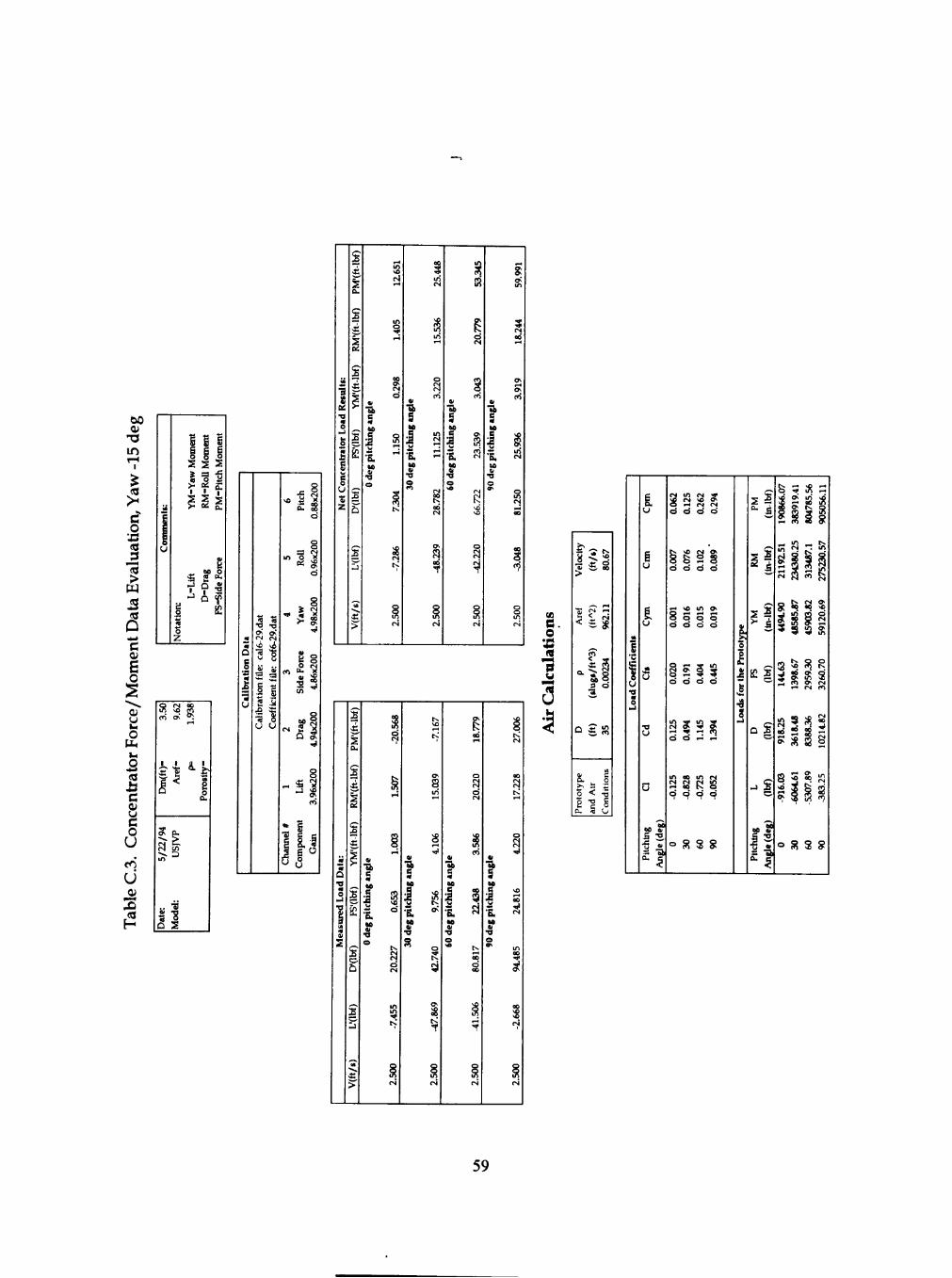
to <ii
in
o •J3 <8 3
1 W B Q *•> c 0)
u 1^ O
U H Wi
(0
C
o U CO
u 3 f2
(0
(J
-Yaw
Mom
ent
-Rol
l M
omen
t •P
itch
Mom
ent
lis >• 06 j i .
Not
atio
n; L
-Lif
t D
-Dra
g F
S-Si
de F
orce
m
Cal
ibra
tion
D
5 S -a -a OL OL IN CN v i vii
ratio
n fil
e: c
al
icie
nt f
ile:
cof
alib
oe
ft
u u
o
^ 2 c: S
o
o o
in ? 2 <« S
o
8
4 Y
aw
4.98
x2
3 Si
de F
orce
4.
86x2
00
o
Cha
nnel
* 1
2 C
ompo
nent
Li
ft D
ra
Gai
n 3.
96x2
00
4.94
x2
esu
lls:
as,
oad
s
Ira
once
n
z
9
CL.
9
(ft-1
s5 ?
(ft-1
^ ***
FS
(Ibf
)
6
Ibf)
J
la
ft/
>
-Sl
S
hin
ri
le
deg
1265
1 40
5 .2
98
o 15
0
r^
304
t^
983 t^
o J?! I N
« -a !: as
chin
pi
l de
g
o
25.4
48
.536
22
0
C l
125
1^ 1-1
.782
0 0 CN
239
-48
ik CM
ai •s, S as
chin
pi
t de
g
o L0
5334
5 77
9
o CN
043
C l
539
S
722
vO vO
220
-42
s I N
ai -a S as
1
pit
ao
o ffL
59.9
91
244
00
919
936
i n CN
250
1^ 0 0
048
*?
o in ( N
It
Q
^
Loa
sure
d
s
ft-l
bf
> > cu
^
ft-
> ^
i « ^ ?
is-1 - .
S£
J b
Ibf)
^
(A
>
•a s
hin|
pi
le
as •fl e
.568
o
^
003
r H
iS d
227
o CN
455
K
500
CM
gle
as
[hin
pi
l<
as •9
s
167
<> 8 i n
106
-i<
« ov
740
9
698
-47
500
cvl
at -ak 1: as
thin
pi
l
as •9 o
779
0 0 1-1
o
Ei o I N
586
en
438
?1
817
o 00
90S
T
500
I N
-ab !3 as
[fain
pi
t
as 01 •« o ov
006
tx I N
00
9 bv r^
220
•«<
816
24.
485
899
rvi
500
I N
o
u
6
ity
X "31 ,>
Are
f
a.
Q
01 a. > O
Prot
^ «
CN
<
cT
ao 9
-3
(ft)
<
and
tv. VO
OO
0023
4
o
in en
? o
Con
I
5 -a
i in CM s -cs o » rH r4 CS
d d d
^O CN o»
8 2 S d d d
1-1 VO i n ^
8 E* 1-" rH
o o o d d d d
o •-• ^ m CN OL O « O - « -W ^
d d d d
S S !Q I f-H ^ rH en d d r r
m flO i n rM s s E: s < 9 =? 9
o S 3 8
s S
82 £ •
o 5 S ^
2
00 ao vo
i §
8 S ffi 3
r - CM C l
m S « 2 8 I
o S 3 8
59

u u O
UH i i 2 <a is c u C o U
U
(2
s Cl
Dm
(ft)
-5/
95
c
ate:
O
VO OL
Are
f-SJ
VP
D
odel
:
S
.938
rH
&.
Por
osit
y-
Q
CaU
brat
ion
^ T3 -o
C-4 CM
'J, ^ •a •«
ratio
n fil
e: c
Ic
ient
file
: c
alib
oe
ft
u u
g
6 Pi
tch
88x2
o
8 in 'S "S
« ^ o
^ 8 " <« i «
-ol
01
3 Si
de F
orc
4.86
x20C
.nS
n\an
nel#
1
2 om
pone
nt
Lift
D
ra
Gai
n 3.
96x2
00
4.94
x2
^ U
(0
3 t
oad
R
lor
I Ir
a 1
Con
cen
« 2
9
ft-l
l M
'(
CL.
9
RM
'(ft-
l
9 r(
ft-i
(I
bf
£
9 f .
b
Ibf)
ZJ
(A
LC
>
Ulg
l •h
in
•R,
deg
e
409
CN 1-1
-0.8
61
0.43
2 84
4
o
662
00
389
t
s in IN
« f as
1 W p
il de
g
s
552
S
-2.3
77
1.20
0
'
501
cvi
o CN VO CM
cn
.524
-5
3
^ in CM
01
? as
chin
pi
l de
g
236
3
-5.6
60
1.18
3
'
823
cn
fS in ON
360
-42
^ in IN
ai
angl
as
chin
pi
t de
g o 9v
076
in
-4.3
83
2906
1
530
cn
o ^0
00 88
2
CN
R in CM
s
S as I
s
-al)
s as
I •Bl as « •a
«
I •B. as
2
ri
c O
u
ity
« •3 >
Are
f
a
D
&
oty
rot
QL.
• ^
(ft
LC
n LC
ao 9 M
(ft)
A
ir
and
t-vo
ii
62.1
OL
0023
4
o
in cn
ons
diti
g u
i.
-I
1.H 9 i n 00
S OO O L ^
- » CM cn d d d d
a CN 00 rH
8 5 8 8 9 ^ d d
CM LO vo > •
8 8 8 S d c <3 d
• * m VO 1 1
s s ^ s d d d d
5 3 S 2 r H iTS r 4 ^ d d 1^ 1^
tN » t>» O.
2 5; K S d c d d
o S 3 8
5? u -
s ^
. |
- ^
CM *0 t^
00 « S Uj rH in ^ "
2 S S 3
I s l 2 8 S S § * •-" ^ 3 v S 2 S g '" " * 2
a § 5; R ^ i ^ ffi <*?
S 3 8
60

to
in r-t
o as 3
1 S & C
U Ui O
IX, I i
2 <s ±s C
o U liS
U (0
H
is
u
III g i 6 S § o s s s %^f >• f E
lis >" * • 0.
01
H ^ as 0 .« 2 B.
L-L
D
-D
-Sid
e
1 e 13 o Z
S C l
-(»
Dm(
22/9
4
^
« D
CN VO OV
1
SJV
P
D
"Z •§
s
.938
L f>
Poro
sI
O e
Ubr
atio
9.
dat
CN
^ •a
ion
f Ue:
ra
t al
ib
u
9.da
t
IN vA
'n U
ent
file:
ic
l
1 u
. 8 ^ •§ s
£ S d
o o
m ? "3 Bi S
O
o o
4 Y
aw
4.98
x2
* m a 8
3 Si
de F
o 4.
86x2
„„8
Cha
nnel
#1
2 C
ompo
nent
Li
ft D
ra
Gai
n 3.
96x2
00
4.94
x2
esu
lls:
K
oad
orL
Ir
al
once
n
elC
X.
v L
M'(
CL,
bf)
ft-
> ^
=? •M
'(ft-1
is i£
5 r-. b
Ibf)
ZJ
• —
L £
>
-ah
s
hin
pi
le
deg
3 r-^
14.
51
-1.0
98
642
o
803
vO
018
K
8 i n I N
01
-ab !3 as
chin
pi
t de
g
o
r H
eo m t^ r-t
-5.1
43
050
K
445
CN
152
-48
8 i n CN
« -a> i as
chin
pi
l d
eg
o «
i n
2
00
o CN
-5.9
65
.635
-1
6 988
i n vO
644
^
g i n CM
01
-ak s ao
rhin
pi
l de
g o ov
i n
R
00
8
-6.7
54
855
-19
790
00
seo
'
s K r4
m
Q •9
Loa
1 s
ft-l
bf)
M'(
Q.
c-
ft-l
b
i
ft-l
bf)
^l"
^
^ g:
. M h
£ ZJ
ft/s
>
s
hing
gp
ilc
•« o
.248
-1
8 02
7
CM
676
r-i
^ t ^
t ^ i n
f-t
161
b v
500
CM
gle
!3 as
hin
•B. as
t l e Cl
«<<
.477
t ^
'
226
VO
597
A.
s 1 - 1 T *
625
500
I N
gle
!3 as
hin
•B. as
•9 e VO
947
ov CM
038
o CV|
465
vO
.124
i n
ov
VO
K
419
-41
500
I N
gle
as
'hin
•iul8
01 •9
O OL
871
cn
.743
vO 1-1
963
vO
392
-17
OO O L f - l
Ov
531
rvi
500
CM
OB
a o
u
6
o
S o c n in
• I Cl Cl o d d
§ i o o o o
m m 9> (o
8 8 8 S d d d d
^ — i n 1-1
S 2 S S
- i fO iC • ^ •"! * "** d r-J i-t
O S.O CN CS CM CM cn i n rH OO K O
d d d d
° S 3 8
=1 5 ; £ S Nil CN i n ^ j ; ^
-: S
^^^s
i 3
iC
8 S
'T •> •? S
a
in t>. C} - -
S I
m cn CM i n
s
« R 2 f-) f ^ ' " .
^ ^
° S 3 8
61
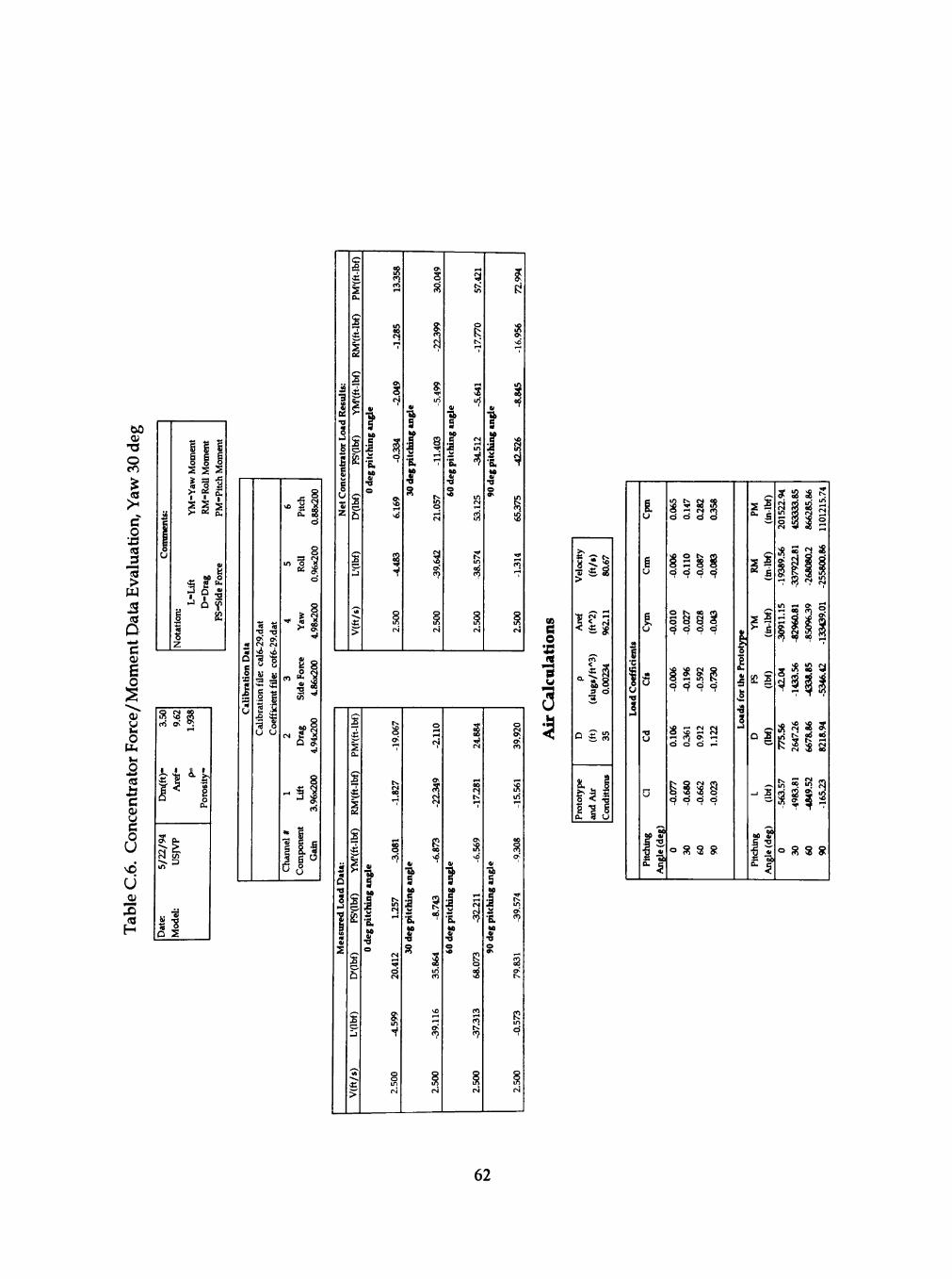
o
I O
•J3 <a 3 I m B «j
D c 0)
u o
OS is c u c O U U X (2
ii
o
-Yaw
Mom
ent
-Rol
l Mom
ent
•Pitc
h M
omen
t
lis > • Otf Cl.
Not
atio
n: L
-Lif
t D
-Dia
g F
S-Si
de F
orce
Cal
ibra
tion
D
^ <a (0
Ov OL' CM CM M!> VA
ratio
n fil
e: c
al
icie
nt fi
le:
cof
Cal
ib
Coe
ff
,. 8 - • ^ 2
0. o8 d
8 in ? "2
« ^ o
8 - ^2 ' * ov
Til
3 Si
de F
orce
4.
86x2
00
Cha
nnel
* 1
2 C
ompo
nent
L
ift
Dra
g G
ain
3.96
x200
4.
94x2
00
s
? I as •8
I V
•B. as
a -a s
I § •B. ^
as •a
R
I as
I •B.
•i ^
-a s
as •s
? as .§ s . 6 CM a CNi
•B. »?
R
§
•I ^
S
OB
o
I
! S S -^ CN cn o d o
9 9 9 9
o r^ 00 m S 8 8 3
9 «^ <=? 9
s s s a rH (TJ O. rH
d o d r
§ §
o S 3 8
I' o I 01 5
s l
1-. 00_ C)
"9 i-J
o6 O. od od K rH
ft • « a
° S 3 8
62
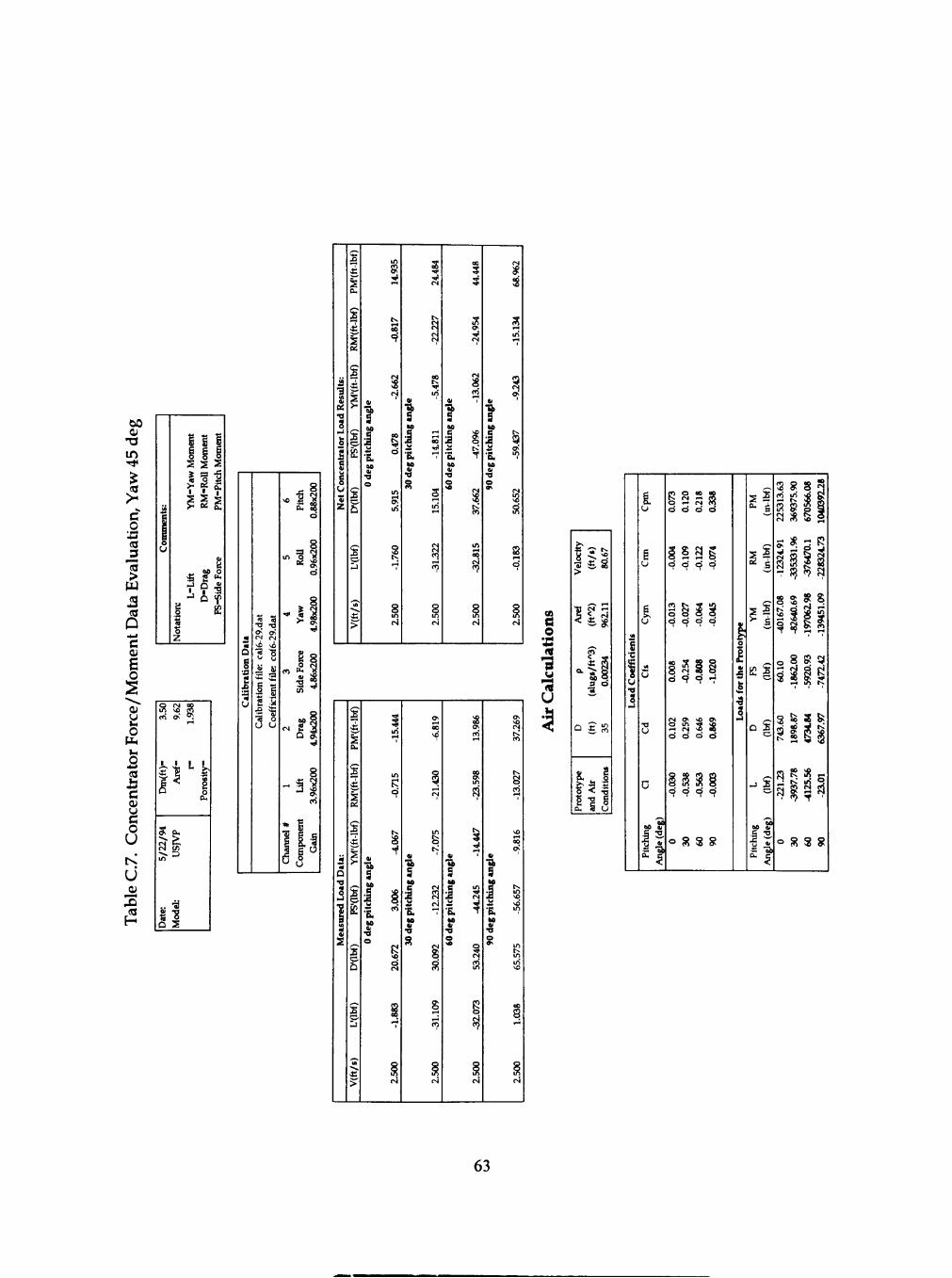
atio
n D
£ t ;
9.da
t 9.
dat
CN CM
vi J>
fUe:
cal
fil
e: c
of
ratio
n ic
ient
al
ib
oeff
U U
8 ^ 1 2
Cu eo o
o o
in f "S •* ov
d
8
4 Y
aw
4.98
x2
3 e Fo
rce
86x2
00
^ ^
. . 8
Cha
nnel
* 1
2 C
ompo
nent
L
ift
Dra
G
ain
3.96
x200
4.
94x2
s
-ab S as
I -B.
-8) S as
I 5 a -t as
TS O
01
-a.
•a -v
s
? as
I
a
•i ^
ffi
I
?;
c O
••c
u
• ^ - r H < •S « >
II c? < £
o - > ao s «
^ £
^ 1 .
^1
Prot
an
d
1 ^ VO
^
r H 96
21
cS y o
i n
^
diti
fi u
00 ai 5 •"
Cl O 00 00 S CM « Q O pH CM M d d d d
< d <3 c
cn t^ * in
S 8 i s CM
o o d d
8 -N o- 9
8
CM 9> ^ » o in ^ \o rH (N ^ OO d d d d
§ S S § Cf d d d
<= S 3 8
s S 2 8 S g f " ^ s .-H t s . sO JK
!S 8! S i < ^ ^ s (N <*i ^o 53 r-*
CJ
vO
<7
00 OL
rJ
9706
R <«• rvi
ffi
-22
S ^
3945
S S S
8 S
3 2
So 2 & «o" V K ^ m ^
2 5i 2
» gaSrf
o S 3 8
63

PERMISSION TO COPY
In presenting this thesis in partial fulfillment of the requirements for a
master's degree at Texas Tech University OP Texas Tech University Health Sciences
Center, I agree that the Library and my major department shall make it freely
available for research purposes. Permission to copy this thesis for scholarly
purposes may be granted by the Director of the Library or my major professor.
It is understood that any copying or publication of this thesis for financial gain
shall not be allowed without my further written permission and that any user
may be liable for copyright infringement.
Agree (Permission is granted.)
student's Signature ^ Date
Disagree (Permission is not granted.)
Student's Signature Date