Lyons_defense

Sediment Dynamics and a Changing

Climate: An integrated model approach to

evaluating the effects of projected

precipitation changes on sediment

production, transport and deposition at

the watershed scale

Kimberly Lyons Graduate Student, USFSP ESPG

Barnali Dixon, Ph.D. Major Professor

Joseph Smoak, Ph.D. Committee Member

Ryan Moyer, Ph.D. Committee Member

1

Presentation Outline

• Introduction

• Research Justification, Goal and Questions

• Study Area and Period

• Research Framework

• Methods

• Results

• Discussion

• Conclusions

• Limitations and Future

• Color Coding

▫ Total Precipitation

▫ High Intensity Precipitation

▫ Current

▫ Future

▫ Change

2

Introduction: Land, Water and Sediment Dynamics

• In the last 50 years ~1 billion hectares of land have been degraded by water driven erosion. (Brady 2008)

▫ Erosion Detached Particles Runoff Aquatic Systems Channel Routing Sediment Delivery

▫ Sediment Dynamics

Production/Supply

Transport

Deposition

Delivery

Supply Limited

Transport Limited

Modified Broz et al, 2003

3

Sediment Delivery

Sedimentation


• Impacts of Anthropogenic Change to Sediment Dynamics

▫ Biogeochemical Cycles

Carbon

Phosphorous and Nitrogen

Physical Properties

Chemicals

▫ Threaten Human Health, Degrade Aquatic Ecosystems and Impose Economic Costs

http://www.sptimes.comPasco/Storm_also_brings_fis.shtml http://soundwaves.usgs.gov/2004/11 http://www.ncbi.nlm.nih.gov/pmc/articles/PMC1448005 http://online.wsj.com/articles/algae-blooms-water-undrinkable-1407107871 http://ecomerge.blogspot.com/2010/05/rosion-leads-to-famine.html

4


• Impacts of Sediment Dynamics ▫ Global Issue

Not Equally Distributed Mediated at a Local Scale

Modeling and Planning

▫ Particularly High Concern in Coastal Watersheds

Meli . et al 2014 NOAA, 2011

5


• “This is further confirmation of the link between upstream nutrient management decisions and the critical habitats and living resources in the Gulf.” – Robert Magnien,

Ph.D. center director at NOAA’s National Centers for Coastal Ocean Science

Hypoxic Zones

Water Erosion http://www.isric .org /projects/global-assessment-human-induced-soil-degration-glaod https://confluence.furman.edu:8443/pages/viewpage.action?pageId=11502753

6

• Despite the distinct connection

▫ Watershed production, transport and deposition coastal sediment delivery

Little systematic research (Slattery and Phillips, 2011)

No one sediment model can simulate all source to sink processes

Modified from William s 2010

7

Introduction: Knowledge Gaps

Oldman et al. 2009

Syvitski, 2003

Precipitation

Soil

Landuse/ Land Cover

Topography

Soil Detachment

Erosion

Runoff

Sediment Delivery

Sediment Yield

Sedimentation

Slattery & Phillips, 2009

Slattery & Phillips, 2009


• In addition to the Source Sink Knowledge Gap, no one model can simulate sediment dynamics at single storm events and annual precipitation

Sediment Model Temporal Resolution

Sediment River Network model (SedNet) Long-term

Universal Soil Loss Equation (USLE) Annual

Revised Universal Soil Loss Equation (RUSLE) Seasonal/ Annual

Environmental Management Support System (EMSS) Daily

Integrated Water Quantity and Quality Model (IQQM) Daily

Productivity Erosion and Runoff Functions to Evaluate Conservation Techniques (PERFECT) Daily

Modified Universal Soil Loss Equation (MUSLE) Event

Griffith University Erosion System Template (GUEST) Event

Limburg Soil Erosion Model (LISEM) Event

Soil and Water Assessment Tool (SWAT) Continuous Time Step

Areal Nonpoint Source Watershed Environmental Response Simulation (ANSWERS) Continuous Time Step

Agricultural Non-Point Source model (AGNPS) Continuous Time Step

8


• Representing precipitation quantity and intensity in sediment modeling is critical ▫ Energy for detachment

▫ Means for transport: particles channels

▫ Stream capacity and competency

USGS, 2006 http://www.acegeography.com/factors-affecting-river-discharge-gcse.html

9


• Creating a framework to address the Source Sink Knowledge that enables total annual and high intensity precipitation sediment dynamics to be understood could:

▫ Facilitate erosion control practices

▫ Aid in short term development

▫ Allow limited resources to be better allocated

10

http://macinctexas.com/?project=waller-creek-erosion-control http://sidestriplesservices.net/erosion-control/ http://www.britannica.com/topic/contour-farming


• Changes in US precipitation patterns

▫ Average rate: +0.15 in/dec

▫ Frequency of >6 in/day: +40%

• Projected Precipitation Changes

▫ Increase in average annual precipitation

▫ Increase in frequency of high intensity precipitation events

Droute et .al, 2015) https://www.ipcc.ch/publications_and_data/ar4/wg1/en/ch10s10-3-6-1.html

11


• Development and planning must consider the relationship between total annual

and high intensity precipitation under future projected climate conditions. (Allan

and Soden, 2008; Bürger et al., 2013; IPCC, 2013; O’Gormana and Schneiderb, 2013; Wang et al., 2013; Wong, 2014)

https://www3.epa.gov/climatechange/impacts/water.html

12

The lack of sediment modeling as a function of climate change is due mostly to the course resolution of Global Circulation Models (GCM). (Xu C et al., 2005; Zhu et al. 2013)

Statistical and dynamic downscaling increases spatial/temporal resolution.

Dynamic downscaling produces more accurate spatial patterns. (Pinto et al.

2014, Syed et al, 2014)

RCMs are created by dynamically downscaling regional appropriate GCM and are readily available as source code downloads

Downscaled data allows catchment scale analysis to be more accurate. (Chandra et

al., 2015; Wang et al., 2013; Xu C et al., 2005; Zhu et al., 2013)

http://climate4impact.eu/impactportal/help/faq.jsp?q=scenarios

13

Research Justification

• Demand for soil and water resources will increase ▫ Current management and future development is imperative

Decision support tool (DST) could facilitate BMPs and climate change mitigation plans Rainfall Quantity and Intensity

Current and Future Climate

Known Knowledge Gaps Publications Addressing Knowledge Gaps Holistic Modeling of Source Sink Relationships

Slattery and Phillips (2006); Williams (2010(

Distinct Differences in the Temporal Resolution of

Sediment Models

Merritt et al (2003); Nearing et al (2005)

Differences in the Response of Sediment Dynamics to

Changes in the Quantity and Intensity of Precipitation

Nearing and Pruski (2003); Hidalgo et al. (2013); Mukundan R et

al (2013)

Integration of Climate Models and Sediment Models

Pruski and Nearing (2003); Hancock (2009); Hancock (2012);

Mukundan R et al (2013)

Accuracy of Climate Models and Downscaling Techniques Xu C et al. (2005); Hancock (2009); Gutmann (2011); Liu et al.

(2011); Teutschbein et al. (2011); Hancock (2012); Mukundan R et

al (2013); Lespinas et al. (2013); Ding and Ke (2013)

14

Research Goal

• Create a DST for quantifying total annual sediment dynamics and sediment dynamics during high intensity events under present climate conditions and projected future conditions

▫ Combining and modifying multiple models/spatial analysis techniques in a model framework

▫ Developing a holistic watershed conceptualization scheme

15

Research Questions

1. How do sediment dynamics as a function of total precipitation and high intensity precipitation vary under current climate conditions?

2. How will sediment dynamics as a function of total precipitation and high intensity precipitation vary under future climate conditions?

3. How will annual sediment dynamics be altered by projected changes in quantity and intensity?

16

Study Area

• Cobb Creek Watershed ▫ Headwaters of the

Altahmaha ▫ 892 km2

▫ Land use Forested: 50.7 %

Agriculture: 27.8%

Wetlands: 14.8%

▫ Elevation 19m-103m

▫ USEPA 305b and 303d lists Fecal Coliform

Dissolved oxygen

17

http://www.ghland.com/listing/toombs-county-ga

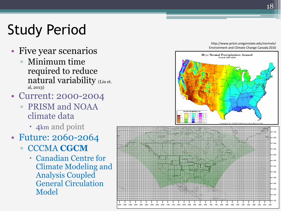
Study Period

• Five year scenarios ▫ Minimum time

required to reduce natural variability (Liu et.

al, 2013)

• Current: 2000-2004 ▫ PRISM and NOAA

climate data

4km and point

• Future: 2060-2064 ▫ CCCMA CGCM

Canadian Centre for Climate Modeling and Analysis Coupled General Circulation Model

18

http://www.prism.oregonstate.edu/normals/ Environment and Climate Change Canada 2016

Research Framework: Model Selection

1. Connect Source to Sink

2. Model Response to Current Total and High Intensity Precipitation

3. Simulate the Effects of Future Climate

4. Holistically Model Sediment Dynamics

19

Research Framework: Source to Sink Models

• Sediment Supply (Terrestrial)

▫ Erosion Model RUSLE Revised Universal Soil

Loss Equation

• Sediment Transport (Terrestrial)

▫ Runoff Model CN Curve Number Method

• Sediment Delivery ▫ In-channel erosion and

routing ▫ Export at watershed

outlet SWAT Soil and Water

Assessment Tool

20

Erosion/Supply/RUSLE

Runoff/ Transport/CN

Sediment Delivery /SWAT

Modified http://www.next.cc/journey/language/watershed

Research Framework: RUSLE Model Description

• Created by the USDA (USDA,

2000)

• Empirical Model

• Based off the well established USLE

▫ Applicable to multiple landuse, topography, and climate (Lu et al. 2004;USDA, 2000)

21

Research Framework: CN Method Description

• Developed by the NRCS

• Empirical equation

▫ Model runoff in ungauged watersheds

22

LanduseHydrologic Soil Group

(HSG)

Empirical Curve Numbers (CN)

(1000/CN)-10

Watershed Storage (S)

Precipitation (P)

(P-0.2S)2 / (P + 0.8S)

Discharge

Research Framework: SWAT Model Description

• Developed by the USDA

▫ Quantify the impact of land management practices

• Two tiered desegregation scheme

• Process/Physical Model

• Continuous Time Step

23

Research Framework: Total and High Intensity

Precipitation Models

24

Process Total Precipitation High Intensity Precipitation

Erosion/Sediment Supply

T-RUSLE (Topographically Modified RUSLE)

I-RUSLE (Intensity Modified T-RUSLE)

Runoff/Sediment Transport

Traditional CN Modified CN

Sediment Delivery SWAT (Annual) SWAT (Daily)

• High Intensity: 50.8 mm/day (Dourte et. al, 2015)

Research Framework: Projected Future Climate

Model

• CGCM ▫ Fourth IPCC Assessment Report

▫ T63 version

▫ Downscaled resolution

.22o lat/lon

12 km

▫ A1B

25

http://sdwebx.worldbank.org/climateppage=country_future_climate_down&ThisRegion=North%20America&ThisCcode=USA

Research Framework: Model Integration

1. Connect Source to Sink

2. Model Response to Current Total and High Intensity Precipitation

3. Simulate the Effects of Future Climate

4. Holistically Model Sediment Dynamics

26

Research Framework: Watershed

Conceptualization

• Terrestrial Sediment Production, Transport and Deposition

• Erosion Detached Particles Runoff Aquatic Systems Channel Routing Sediment Delivery

• Supply/ Transport Potential (Williams et al., 2010)

▫ RUSLE soil loss Sediment Supply Potential

▫ CN Runoff Values Sediment Transport Potential

27

Watershed Supply and Transport Supply and Transport Limitations

• Low Sediment Supply • High Sediment Transport Supply Limited

• High Sediment Supply • Low Sediment Transport Transport Limited

• Low Sediment Supply • Low Sediment Transport Supply and Transport Limited

• High Sediment Supply • High Sediment Transport Not Supply or Transport Limited

Research Framework: Watershed

Conceptualization

• Low/ Moderately Low Redistribution Potential ▫ Minimum Delivery Potential

• Moderate Redistribution Potential

• Moderately High/High Redistribution Potential ▫ Maximum Delivery Potential

28

Combinations of Production and Transport Potentials

Combined Values

Redistribution Potential

• Low Transport + Low Production -2 Low

• Low Transport + Moderate Production • Moderate Transport + Low Production -1 Moderately Low

• Moderate Transport + Moderate Production • High Transport + Low Production • Low Transport + High Production 0 Moderate

• High Transport+ Moderate Production • Moderate Transport + High Production 1 Moderately High

• High Sediment Transport+ High Sediment Production 2 High

Research

Framework: Watershed

Conceptualization

• Linking Terrestrial Sediment Dynamics to Sediment Delivery

▫ Assumption: Combined terrestrial sediment supply and transport (Redistribution Potential) will be reflected temporally in SWAT model results

Quantity= Annual

Intensity= Daily

29

Erosion Detached Particles Runoff Aquatic Systems Channel Routing Sediment Delivery

Topographic Modified: T- RUSLE

Land Cover Factor (C)

Soil Erodiblity Factor (K)

Rainfall/ Runoff Factor

(R)

Soil Conservation

Factor (P) LS Factor

RUSLEA=R*K*LS*C*P

Average Annual Soil Erosion

Slope Curvature Multiplier

(SCM

Intensity Modified: I- RUSLE

Land Cover Factor (C)

Soil Erodiblity Factor (K)

Rainfall/ Runoff Factor

(R)

Soil Conservation

Factor (P) LS Factor

RUSLEA=R*K*LS*C*P

Average Annual Soil Erosion: Emphasis on High Intensity Precipitation

Rainfall Intensity

Multiplier (RIM)

Slope Curvature Multiplier

(SCM

Slope Curvature Multiplier (SCM) Classifications

Slope Curvature Values

Slope Shape Slope Type Slope Effect Rating

<0 Convex Erosional 1.5

0 Flat Transitional 0

>0 Concave Depositional 0.5

Methods: Sediment

Supply Modeling

30

• ArcGIS 10.1

• Traditional Factors

▫ USDA Agricultural Handbook (2000)

• SCM

▫ Slope Curvature Reclassify Slope Effect Rating

• RIM

▫ (Total High Intensity/ Annual Average Total) +1

Matlab 2014R

• Landscape factors held constant

Methods: Sediment

Supply Modeling

• Erosion Model Equations and Precipitation Inputs

31

T-RUSLE and I-RUSLE Equations

Scenarios Model Equations

Current Climate

T- RUSLE LS*K*C*P*SCM*RCURRENT

I-RUSLE LS*K*C*P*SCM*RCURRENT*RIMCURRENT

Future Climate

T- RUSLE LS*K*C*P*SCM*RFUTURE

I-RUSLE LS*K*C*P*SCM*RFUTURE*RIMFUTURE

Methods: Terrestrial Sediment Transport Modeling

• Procedure outlined in NRCS Technical Report-55 (1986) • High Intensity Modified: RIM calculated for I-RUSLE

32

Example CN Workflow: Current Climate Total Precipitation

Methods: Sediment Delivery Model Simulations

• ArcSWAT 2012

▫ Procedure Outlined in SWAT User Manual (2012)

▫ Minor changes to default setting

• Total Precipitation

▫ Annual

• High Intensity Precipitation

▫ Daily

▫ >50.8 mm/day

• Future Climate

▫ Chen et al., 2015

33

Methods: Sediment Delivery Model Calibration/

Validation

• Contour and Test

▫ Adjust parameters

▫ Simulated v Observed

• SWATCup

▫ Semi-automated calibration software

• Daily Discharge

▫ PBIAS: Average tendency of the simulated data to be larger or smaller than observed

0.98/0.99 (Goal 0)

• Monthly Sediment Load

▫ Nash–Sutcliffe Efficiency: Normalized statistic used to compare the residual variance to data variance

0.62/.087 (Goal 1)

34

Parameter Bounds Calibrated Value

Parameters Related to Runoff and Steam Flow

CN2.mgt ± 0.2 +0.174

ALPHA_BF.gw 0.0 - 1.0 0.0404

GW_DELAY.gw 0 – 400 24.76

GWQMN.gw 0 – 500 56.77

ESCO.hru 0.5 - 0.95 0.926

RCHRG_DP.gw 0 – 1 0.544

SURLAG.bsn 0 – 10 6.56

GW_REVAP.gw 0.02 – 2 0.077

REVAPMN.gw 0 – 500 195.33

SOL_AWC().sol ±0.2 -0.055

CH_K2.rte 0.01 – 150 11.08

Parameters Related to Sediments

SPCON 0.001- 0.002 0.004

CH_EROMO 0.12-0.14 .127

SPEXP 1.35-1.47 1.37

Methods: Sediment Delivery Model Calibration/

Validation

• Example of Model Performance

▫ Observed

▫ Simulated

▫ Model Uncertainty

• “Satisfactory” to “Good”

35

Methods: Terrestrial Model Integration Baseline

• Baseline for Classifications ▫ Current Total Precipitation Model

Jenks Natural Breaks

Modified Baseline: Future CN

36

Classification

Sediment Supply/Transport

Potential Definition

-1 Low Sediment Supply/

Transport

0 Moderate Sediment Supply/Transport

1 High Sediment Supply/

Transport

CN TP Current

Jenks Natural Breals

Baseline CN Current

Classification

Baseline CN Future

Classification

Magnitude adjustment

(1.7)

RUS TP FCurrent

Jenks Natural Breals

Baseline RUSLE

Classification

37

-2

2

-1

0

1

-1

-1

0

0

1

1

Methods: Terrestrial Model Integration

Methods: Statistical Analysis

• Matlab 2014R

• Assumptions

▫ All Models: Non-Parametric: Shapiro-Wilks (a0.05)

▫ Terrestrial Models: Paired- Dependent

38

Statistical Test Compared Data

Mann–Whitney (SWAT) H0: There is no significant difference in the central tendency of model values under total and high intensity precipitation simulations

• Total v High Intensity Sediment Delivery

Wilcoxon Sign Rank (Terrestrial Models) H0: There is no statistical difference in the central tendency of model values under total and high intensity precipitation simulations

• Total v High Intensity Sediment Supply Classifications

• Total v High Intensity Sediment Transport Classifications

• Total v High Intensity Source/ Sink Classifications

Current Climate: Total v High Intensity Precipitation Sediment Dynamics AND Future Climate: Total v High Intensity Precipitation Sediment Dynamics

Methods: Statistical Analysis

39

Statistical Test Compared Data

Mann–Whitney (SWAT) H0: There is no significant difference in the central tendency of model values under current and future climate conditions

• Current v Future Total Precipitation Sediment Delivery • Current v Future High Intensity Sediment Delivery

Wilcoxon Sign Rank (Terrestrial Models) H0: There is no statistical difference in the central tendency of model values under current and future climate conditions

• Current v Future T-RUSLE • Current v Future I-RUSLE • Current v Future Annual CN • Current v Future Modified CN • Current v Future Total Precipitation Sediment Supply

Classifications • Current v Future High Intensity Sediment Supply Classifications • Current v Future Total Precipitation Sediment Transport

Classifications • Current v Future High Intensity Sediment Transport Classifications • Current v Future Total Precipitation Sorce/Sink Classifications • Current v Future High Intensity Source/Sink Classifications

Current v Future Total Precipitation Sediment Dynamics AND Current v Future High Intensity Precipitation Sediment Dynamics

Methods: Spatial Analysis

• Terrestrial Models

▫ ArcGIS 10.1

▫ Watershed Classification Differences

Statistically Significant

Spatial Distribution of Change

▫ Percentage Change Analysis

40

Model A

Model B

Increase

High Intensity – Total Future Climate – Current Climate

Erosion/Supply/RUSLE

Runoff/ Transport/CN

Sediment Delivery /SWAT

Methods: Temporal Analysis

• SWAT Model

▫ Graphical Analysis

Excel 2013

▫ Visualize ‘event’ based nature of watershed sediment dynamics

Current and Future Climate Sediment Delivery Patterns in the temporal distribution

Contribution of high intensity precipitation

Compare current and future sediment delivery Magnitude, variability and temporal distribution

41

Methods: Primary Data

• Landscape Features

42

Methods: Primary Data

43

• Precipitation

Results: Ho- There is no significant difference in the central

tendency of model values under total and high intensity

precipitation simulations

Current Climate

Pairwise Comparison Test Statistic P-value

Wilcoxon Matched Pairs Analysis

T-RUSLE v I-RUSLE 2.33 0.02

Annual CN v Modified CN 120.53 <0.001

Total v High Intensity Sediment Supply Classifications 1.42 0.15

Total v High Intensity Sediment Transport Classifications 54.99 <0.001

Total v High Intensity Redistribution Classifications 47.21 <0.001

Mann–Whitney Analysis

Total v High Intensity Sediment Delivery 17.6 0.015

44

Future Climate Analysis

Pairwise Comparison Test Statistic P-value

Wilcoxon Matched Pairs Analysis

T-RUSLE v I-RUSLE 25.55 <0.001

Annual CN v Modified CN 930.15 <0.001

Total v High Intensity Sediment Supply Classifications 11.42 <0.001

Total v High Intensity Sediment Transport Classifications 388.39 <0.001

Total v High Intensity Redistribution Classifications 286.4 <0.001


Total v High Intensity Sediment Delivery 18.7 0.01

Results: H0- There is no significant difference in the central

tendency of model values under current and future climate

conditions

45

Current and Future Climate Matched Pairs Analysis

Pairwise Comparison Test Statistic P-value Wilcoxon Matched Pairs Analysis

Current v Future T-RUSLE 60.22 <0.001

Current v Future I-RUSLE 81.65 <0.001

Current v Future Annual CN 1055.4 <0.001

Current v Future Modified CN 1055.6 <0.001

Current v Future Total Precipitation Sediment Supply Classifications 37.66 <0.001

Current v Future High Intensity Sediment Supply Classifications 47.5 <0.001

Current v Future Total Precipitation Sediment Transport Classifications 65.57 <0.001

Current v Future High Intensity Sediment Transport Classifications 385.95 <0.001

Current v Future Total Precipitation Redistribution Classifications 80.45 <0.001

Current v Future High Intensity Redistribution Classifications 319.67 <0.001


Current v Future Total Annual Precipitation Sediment Delivery 20.4 0.001

Current v Future High Intensity Sediment Delivery 20.1 0.001

Results: RQ-1 Current Climate

• Sediment Supply Potential

▫ Total Precipitation and High Intensity Precipitation

Low Potential

46

T-RUSLE I-RUSLE


• Sediment Transport Potential


High/ Moderately High Potential

▫ Increase in 4.2% Watershed: ~37 km2

Localized to SW

47



• Sediment Transport Potential


High/ Moderately High Potential

▫ Increase in 4.2% Watershed: ~37 km2

Localized to SW

48


• Sediment Redistribution Potential


Few ‘Hotspots’ or Terrestrial ‘Stores’

Moderately Low to Moderate Potential

▫ Up to 2 Class Increase

3.9% Watershed: ~35 km2

49

T-RUSLE and Traditional CN I-RUSLE and Modified CN


Results: RQ-1 Current

Climate

• Sediment Delivery


Average Annual: ~130,000 tonnes/yr

▫ High Intensity Precipitation (Contribution)

9 Events

Late Summer / Early Fall

Average Annual: ~37,000 tonnes/yr (29%)

2001: No Events = No Contribution

6%-65%

Max Event: 111,000

tonnes/day

50

Results: RQ-2 Future Climate

• Sediment Supply Potential ▫ Total Precipitation and High

Intensity Precipitation

Low Potential

▫ Patchy Increase in 0.8% Watershed: ~7 km2

S bank of main channel

51

T-RUSLE I-RUSLE


• Sediment Transport

Potential

▫ Total Precipitation: High/ Moderately High Potential

▫ High Intensity: High Potential

▫ Increase in 23.1% watershed: ~206 km2

High change density NW

Area of no supply change effected

52



• Sediment Redistribution

Potential ▫ Total Precipitation: Moderately Low/

Moderate

▫ High Intensity: Moderate 3% ‘Hotspot’:~ 33 km2

No Terrestrial ‘Stores’

▫ Increase in 20.4% watershed: ~182 km2

Most Prevalent in NW

53

T-RUSLE and Traditional CN I-RUSLE and Modified CN

Results: RQ-2 Future

Climate

• Sediment Delivery


Average Annual: ~ 350,000 tonnes/yr


(Contribution)

11 Events

Winter

Multiple Storms/ yr

Average Annual:

150,000 tonnes/yr (43%)

2062: No events= no contribution

20%-60%

Max Event:

148,000 tonnes/day

54

Results: RQ-3 Climate Change

• Total Precipitation Sediment Supply

▫ Increase in Soil Erosion

Max: +814 tonnes ha-1 yr-1

Mean: +2.5 tonnes ha-1 yr-1

▫ Increase in Potential

1.9% Watershed Area

~17 km2

Primarily

N Main Channel

Row Crop Landuse

55

Current and Future T-RUSLE


• Total Precipitation Sediment Transport ▫ Increase in Runoff

Max: +608 mm/yr

Mean: +547.7 mm/yr

▫ Change in Potential

4.0% Watershed Area

~34 km2 Increase/~2 km2

decrease

Primarily E Edge

Decrease NE and SW edges

56

Current and Future Traditional CN


• Total Precipitation Sediment Transport ▫ Increase in Runoff

Max: +608 mm/yr

Mean: +547.7 mm/yr

▫ Change in Potential

4.0% Watershed Area

~34 km2 Increase/~2 km2

decrease

Primarily E Edge

Decrease NE and SW edges

57

Current and Future Traditional CN

Results: RQ-3 Climate

Change

• Total Precipitation Sediment Redistribution Potential

▫ Change in 4.3% Land Area

~36 km2 increase/2 km2 decrease

▫ Primary E Edge

58

Current and Future T-RUSLE and Traditional CN

Results: RQ-3 Climate

Change

59

• Total Precipitation Sediment Delivery ▫ Average Annual

Future ~2.7x Current

▫ Max Annual

Future ~3x Current

▫ Increased Variability

Current and Future Annual SWAT

Annual Sediment Delivery for Five Years of Simulation (Tonnes/Year)

Simulation Current Future

Year 1 172,800 517,200

Year 2 74,560 256,900

Year 3 103,100 149,700

Year 4 184,900 452,400

Year 5 109,300 380,600

Average 128,932 351,360


• High Intensity Precipitation Sediment Supply

▫ Soil Erosion Increase

Max: +510 tonnes ha-1 yr-1

Mean: +15.21 tonnes ha-1 yr-1


2.4% of Watershed

~21 km2

Primarily

N Main Channel

Row Crop and

Hay Pasture

60

Current and Future I-RUSLE


• High Intensity Precipitation Sediment Transport Potential

▫ Increase in Runoff

Max: +935 mm/yr

Mean: +681.2 mm/yr


21.1% Watershed Area

~188 km2

Least Dense NE and SW

61

Current and Future Modified CN


• High Intensity Precipitation Sediment Redistribution Potential

▫ 22.8% Watershed Area

~203 km2

▫ Least Change in SW

Already Impacted by High Intensity

62

Current and Future I-RUSLE and Modified CN


63

• High Intensity Precipitation Sediment Delivery ▫ Average Annual: Future~4x Current

▫ Event Max: Future ~1.7x Current

▫ Shift in dominate season

▫ Increased frequency of high sediment delivery events

Sediment Delivery from High Intensity

Precipitation for Five Years of Simulations

Date Tonnes/ Day

Date Tonnes/ Day

3/30/00 111,000 2/7/60 64,740

8/30/02 6,274 2/17/60 96,150

6/17/03 4,362 12/18/60 68,030

7/24/03 5,989 12/31/60 67,250

9/6/03 16,360 12/22/61 6,633

10/26/03 6,487 1/9/63 13,630

9/6/04 15,390 1/23/63 66,860

9/7/04 8,317 7/16/63 39,220

9/27/04 10,950 7/17/63 49,200

12/11/64 147,600

12/23/64 130,000

Average 20,570 Average 68,119

Current and Future Daily SWAT

Discussion: RQ-1 and RQ-2

• How do sediment dynamics as a function of total precipitation and high intensity precipitation compare under current climate conditions? ▫ SW Watershed

▫ Fall

• How will sediment dynamics as a function of total precipitation and high intensity precipitation vary under future climate conditions? ▫ Entire watershed: Most prevalent NW

watershed

▫ Winter

• Hydrography ▫ Distance Buffers

▫ Within Watershed Aquatic Sinks

▫ In Stream Travel Distance

64

Area Most Effected by High Intensity: Future

Area Most Effected by High Intensity: Current


• Landuse/ Land Cover

▫ Vegetation Buffers

▫ Variations in BMPs

▫ Seasonality Temporal Variation of

Landuse NOT simulated

Tillage, Irrigation, Offseason Erosion Controls, Temperature, Leaf Loss

65

Area Most Effected by High Intensity: Future

Area Most Effected by High Intensity: Current


• High intensity precipitation will play a greater role in annual sediment dynamics under future projected climate conditions

66

Differences in Total and High Intensity Precipitation Sediment Dynamics

Sediment Process Current Climate Future Climate Comparison of Area Effected by

High Intensity Precipitation

Supply Not Significant 0.08% Watershed

Area Future ~8x (6 km2) current area

affected

Transport 4.2% Watershed

Area 23.1% Watershed

Area ~6x (150 km2) more than current

climate conditions

Supply and

Transport 3.9% Watershed

Area 20.4% Watershed

Area Future ~5x (145 km2) more than

current climate conditions

Sediment Delivery 29% of Average

Annual Sediment

Delivery

43% of Average

Annual Sediment

Delivery

14% more contribution than current

climate conditions

Discussion: RQ-3

• How will total annual sediment dynamics and sediment dynamics during high intensity precipitation events be affected by climate change?

▫ Total precipitation sediment dynamics will increase

E Watershed

▫ High intensity precipitation sediment dynamics will increase

N and E Watershed

Fall to Winter

67

Differences in Current and Future Sediment Dynamics

Sediment Process Total Precipitation High Intensity Precipitation

Supply 1.9% Watershed Area 2.4% Watershed Area

Transport 4.0% Watershed Area 21.1% Watershed Area

Supply and Transport 4.3% Watershed Area 22.8% Watershed Area

Discussion: RQ-3

• Total Precipitation

▫ Already Area of High Sediment Potential

▫ Hydrography

High Channel Density

In Watershed Aquatic Sinks

▫ Landsue

Only Urbanized Area

Urban Runoff and Flashiness

• High Intensity Precipitation

▫ Entire Watershed Area

68

Discussion: Implications

• Watershed has large potential for development

▫ >60% undeveloped

• Under current landuse climate change could

1. Reduce agricultural productivity

2. Degrade water quality

3. Negatively impact watershed wetlands

4. Increase export of sediments, nutrients and chemicals to downstream waters

Altahmaha 3rd largest contributor to Atlantic in N. America

1/3 of GA fisheries (Isley, 2003; USDI et al., 2011)

2nd largest waterfowl management area in eastern US (GADNR, 2011)

69

Discussion: Management Suggestions

• Current Practices

▫ Total Precipitation BMPs

NE part of watershed

High total precipitation, midrange elevation, agriculture

▫ High Intensity Precipitation BMPs

SW watershed

Late summer and early fall

• Future Practices

▫ Total precipitation BMPs

E half watershed

▫ High Intensity Precipitation BMPs

Entirety of watershed

Winter

▫ N focus on erosion control

▫ Long term infrastructure development

Larger annual

More extreme sediment loads

70

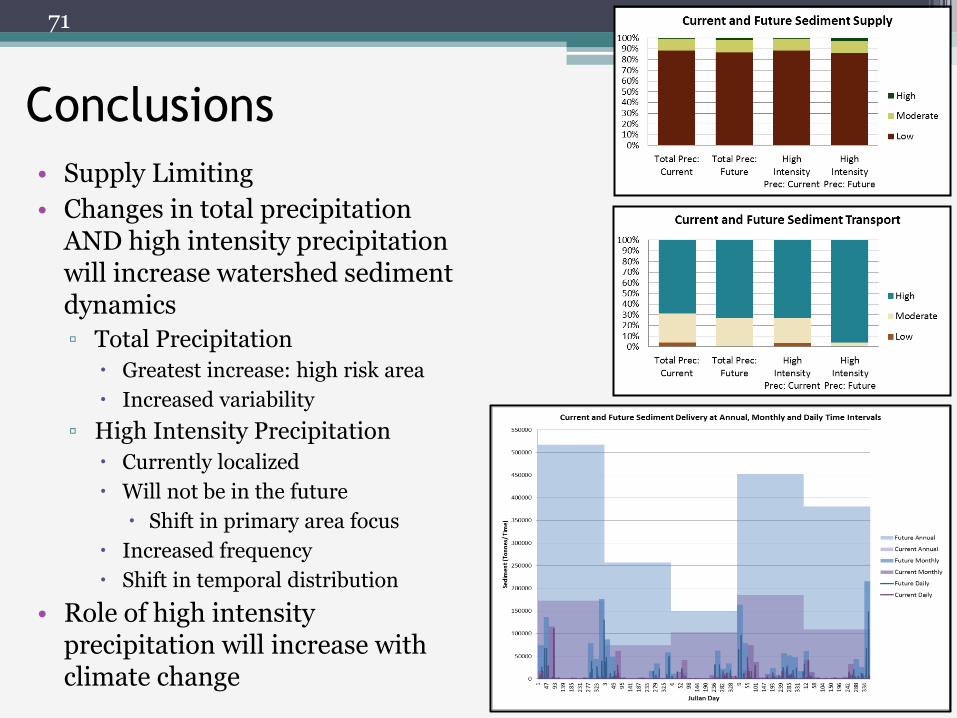
Conclusions

• Supply Limiting

• Changes in total precipitation AND high intensity precipitation will increase watershed sediment dynamics


Greatest increase: high risk area

Increased variability


Currently localized

Will not be in the future

Shift in primary area focus

Increased frequency

Shift in temporal distribution

• Role of high intensity precipitation will increase with climate change

71

Conclusions

• Sediment Dynamics

▫ Are different under total precipitation and high intensity precipitation

▫ Respond differently to projected changes in total precipitation and the frequency and intensity of rainfall

• Results (Cobb Creek Watershed)

▫ Current climate BPMs

▫ Develop climate change adaptation and mitigation strategies

• Model framework /watershed conceptualization scheme could be used as a DST in other watersheds

72

Framework Limitations and Future Research

73

Representation of Time

High Intensity Modifications ≠ Single Storm Event

Event Models in Place of Modified Models

Definition of High Intensity Modify Time Intervals • Include Lag Time Multiple Subbasin Analysis Different Definitions

Land Cover/ Landuse: Seasonality Seasonally Contour SWAT Inputs

Land Cover/ Landuse: Development Incorporate Land Change Model

Data Availability

Calibration/Validation Data Collection for Terrestrial Component Validation

User Exclusions

Data Resolution

Landscape parameters: 30mx30m

Precipitation • Current: 4kmx4km

• Future: 12kmx12km

Additional Downscaling

Future Climate Model Compounding Uncertainty

GCM + Downscaling + Emission Scenario Multiple Emission Scenarios and RCMs

Acknowledgements

• USF Environmental Science and Policy Program

• Advisor and Mentor: Dr. Barnali Dixon

• The Geospatial Analytics Lab

• Committee Members: Joseph aka “Donny” Smoak and Ryan Moyer

• My loving family and dear friends

74

75

?????

References • Abell, R. A. (2000). Freshwater ecoregions of North America : A conservation assessment. Washington, D.C.: Island Press.

• Adams, H. D., Williams, A., Xu, C., Rauscher, S., Jiang, X., & McDowell, N. (2013). Empirical and process-based approaches to climate-induced forest mortality models. Frontiers in Plant Science, 4, 438.

• Ahmadi, S. H., Amin, S., Reza Keshavarzi, A., & Mirzamostafa, N. (2006). Simulating watershed outlet sediment concentration using the ANSWERS model by applying two sediment transport capacity equations. Biosystems Engineering, 94, 615-626.

• Aksoy, H., & Kavvas, M. (2005). A review of hillslope and watershed scale erosion and sediment transport models. Catena, 64(25), 247-271.

• Allan, R. P. & Soden, B. J. (2008). Atmospheric warming and the amplification of precipitation extremes. Science, 321.

• Andersson, J., & Nyberg, L. (2008). Relations between topography, wetlands, vegetation cover and stream water chemistry in boreal headwater catchments in Sweden. Hydrology & Earth System Sciences Discussions, 5(3), 1191-1226.

• Anthony, E. J., & Julian, M. (1999). Source-to-sink sediment transfers, environmental engineering and hazard mitigation in the steep river catchment, French Riviera, southeastern France. Geomorphology, 31(1–4), 337-354.

• ArcSWAT 2012.10.15 [Computer software]. (2014). College Station, TX: Texas A&M University. Retrieved from http://swat.tamu.edu/software/arcswat.

• Arienzo, M., Masuccio, A., & Ferrara, L. (2013). Evaluation of sediment contamination by heavy metals, organochlorinated pesticides, and polycyclic aromatic hydrocarbons in the Berre coastal lagoon (southeast France). Archives of Environmental Contamination & Toxicology, 65(3), 396-406.

• Arnbjerg-Nielsen, K., Willems, P., Olsson, J., Beecham, S., Pathirana, A., Bülow Gregersen, I., & Nguyen, V. (2013). Impacts of climate change on rainfall extremes and urban drainage systems: A review. Water Science & Technology, 68(1), 16-28.

• Arnold, J.G., Kiniry, J., Srinivasan, R., Williams, J., Haney, & E., Neitsch, S. (2011). Soil and Water Assessment Tool "SWAT". Texas Water Resources Institute TR- 439.

• Bauer, J. E., Cai, W., Raymond, P., Bianchi, T., Hopkinson, C., & Regnier, P. (2013). The changing carbon cycle of the coastal ocean. Nature, 504(7478), 61-70.

• Bennett, N. D., Croke, B., Guariso, G., Guillaume, J., Hamilton, S., Jakeman, A., & Andreassian, V. (2013). Characterizing performance of environmental models. Environmental Modelling and Software, 40, 1-20.

• Bianchi, T. S., Garcia-Tigreros, F., Yvon-Lewis, S., Shields, M., Mills, H., Butman, D., & Grossman, E. (2013). Enhanced transfer of terrestrially derived carbon to the atmosphere in a flooding event. Geophysical Research Letters, 40(1), 116-122.

• Booij, M. J., Tollenaar, D., van Beek, E., & Kwadijk, J. (2011). Simulating impacts of climate change on river discharges in the Nile basin. Physics and Chemistry of the Earth, 36, 696-709.

• Brady, N. C. & Weil, R. R. (2008) Nature and Properties of Soil. Pearson.

• Brierley, G. J., & Fryirs, K. A. (2008). River futures: An integrative scientific approach to river repair. Washington D.C.: Island Press.

• Bürger, G., Sobie, S., Cannon, A., Werner, A., & Murdock, T. (2013). Downscaling extremes: An intercomparison of multiple methods for future climate. Journal of Climate, 26(10), 3429-3449.

• Cao, W., Bowden, W., Davie, T., & Fenemor, A. (2006). Multi-variable and multi-site calibration and validation of SWAT in a large mountainous catchment with high spatial variability. Hydrological Processes, 20(5), 1057-1073.

• Chandra, R., Saha, U., & Mujumdar, P. (2015). Model and parameter uncertainty in IDF relationships under climate change. Advances in Water Resources, 79, 127-139.

• Chandramohan, T., Venkatesh, B., & Balchand, A. (2015). Evaluation of three soil erosion models for small watersheds. Aquatic Procedia, 4, 1227-1234.

• Chen, X., Alizad, K., Wang, D., & Hagen, S. (2014). Climate change impact on runoff and sediment loads to the Apalachicola river at seasonal and event scales. Journal of Coastal Research, 68, 35-42.

• Daniels, J. A. (2012). Advances in environmental research. New York: Nova Science Publishers, Inc.

• Ding, T., & Ke, Z. (2013). A comparison of statistical approaches for seasonal precipitation prediction in Pakistan. Weather & Forecasting, 28(5), 1116-1132.

• Diplas, P., Kuhnle, R., Gray, J., Glysson, D., & Edwards, T. (2008). Sediment Transport Measurements. Water Resources: United States Geologic Survey.

• Dourte, D. R., Fraisse, C., & Bartels, W. (2015). Exploring changes in rainfall intensity and seasonal variability in the southeastern U.S.: Stakeholder engagement, observations, and adaptation. Climate Risk Management, 7, 11-19.

• Dumas, P., Printemps, J., Mangeas, M., & Luneau, G. (2010). Developing erosion models for integrated coastal zone management: A case study of the New Caledonia west coast. Marine Pollution Bulletin, 61, 519-529.

76

References • Eslamian, S. (2014). Handbook of engineering hydrology : Environmental hydrology and water management. Boca Raton, FL: CRC Press.

• Feiner, P., Dlugo, V., & Van Oost, K. (2015). Erosion-induced carbon redistribution, burial and mineralisation — is the episodic nature of erosion processes important? Catena, 133, 282-292.

• Feser, F., Rockel, B., von Storch, H., Winterfeldt, J., & Zahn, M. (2011). Regional climate models add value to global model data: A review and selected examples. Bulletin of the American Meteorological Society, 92(9), 1181-1192.

• Fu, B., Chen, L., Ma, K., Zhou, H., & Wang, J. (2000). The relationships between land use and soil conditions in the hilly area of the loess plateau in northern Shaanxi, China. Catena, 39, 69-78.

• Fujita, M., Yamanoi, K., & Izumiyama, H. (2014). A combined model of sediment production, supply and transport. Iahs Publication, 367357-36.

• Furl, C., Sharif, H., & Jeong, J. (2015). Analysis and simulation of large erosion events at central texas unit source watersheds. Journal of Hydrology, 527, 494-504.

• Gajbhiye, S., & Mishra, S. K. (2012). Application of NRSC-SCS curve number model in runoff estimation using RS & GIS. IEEE-International Conference on Advances in Engineering, Science & Management (ICAESM -2012), 346.

• Gao, P. (2011). An equation for bed-load transport capacities in gravel-bed rivers. Journal of Hydrology, 402, 297-305.

• GDNREPD & USUSEPA. (2002). Fecal Coliform TMDLs: Altamaha River Basin.

• Georgia Department of Natural Resources Environmental Protection Division and U.S. Environmental Protection Agency, Region 4.

• GDNREPD & USEPA. (2002). Total Mercury TMDLs: Altamaha River Basin.

• Georgia Department of Natural Resources Environmental Protection Division and U.S. Environmental Protection Agency, Region 4.

• GDNREPD & USEPA. (2002). Total Mercury in Fish Tissue Residue: Altamaha River Basin. Georgia Department of Natural Resources Environmental Protection Division and U.S. Environmental Protection Agency, Region 4.

• GDNREPD & USEPA. (2007). Dissolved Oxygen TMDLs. Altamaha River Basin Impaired Streams Evaluation. Georgia Department of Natural Resources Environmental Protection Division and U.S. Environmental Protection Agency, Region 4.

• eorgia Department of Natural Resources Environmental Protection Division and U.S. Environmental Protection Agency, Region 4.

• GDNREPD & USEPA. (2012). Fecal Coliform TMDLs. Altamaha River Basin Impaired Streams Evaluation. Georgia Department of Natural Resources Environmental Protection Division and U.S. Environmental Protection Agency, Region 4.

• GDNREPD & USEPA. (2012). Sediment (Biota Impacted) TMDLs. Altamaha River Basin Impaired Streams Evaluation. Georgia Department of Natural Resources Environmental Protection Division and U.S. Environmental Protection Agency, Region 4.

• Gebremariam, S. Y., Martin, J., DeMarchi, C., Bosch, N., Confesor, R., & Ludsin, S. (2014). A comprehensive approach to evaluating watershed models for predicting river flow regimes critical to downstream ecosystem services. Environmental Modelling and Software, 61, 121-134.

• Guntermann, K. L., Lee, M., & Swanson, E. (1976). The economics of off-site erosion. Annals of Regional Science, 10(3), 117.

• Hargreaves, G. H., & Allen, R. G. (2003). History and evaluation of Hargreaves evapotranspiration equation. Journal Of Irrigation & Drainage Engineering, 129(1), 53.

• SWAT Check 1.1.15 [Computer software]. (2014). College Station, TX: Texas A&M University. Retrieved from http://swat.tamu.edu/software/swat-check.

• SWAT-Cup 5.1.6.1 [Computer software]. (2014). College Station, TX: Texas A&M University. Retrieved from http://swat.tamu.edu/software/swat-cup.

• Swiss Federal Institute of Aquatic Science and Technology. (2015). SWAT-Cup: SWAT calibration and uncertainty programs- a user manual. EAWAG.

• Syed, F., Iqbal, W., Syed, A., & Rasul, G. (2014). Uncertainties in the regional climate models simulations of South-Asian summer monsoon and climate change. Climate Dynamics, 42(7), 2079-2097.

• Teng, J., Potter, N., Chiew, F., Zhang, L., Vaze, J., & Evans, J. (2014). How does bias correction of RCM precipitation affect modelled runoff? Hydrology & Earth System Sciences Discussions, 11(9), 10683-10724.

77

References • Teutschbein, C., Wetterhall, F., & Seibert, J. (2011). Evaluation of different downscaling techniques for hydrological climate-change impact studies at the catchment scale.

Climate Dynamics, 37(9), 2087-2105.

• Thrush, S. F., Hewitt, J., Cummings, V., Ellis, J., Hatton, C., Lohrer, A., & Norkko, A. (2004). Muddy waters: Elevating sediment input to coastal and estuarine habitats. Ecological Society of America.

• Tian, D., Martinez, C., Graham, W., & Hwang, S. (2014). Statistical downscaling multimodel forecasts for seasonal precipitation and surface temperature over the southeastern United States. Journal of Climate, 27(22), 8384-8411.

• Timbal, B., Hope, P., & Charles, S. (2008). Evaluating the consistency between statistically downscaled and global dynamical model climate change projections. Journal of Climate, 21(22), 6052-6059.

• USDA. (1978). Predicting Rainfall Erosion losses: A guide to Conservation Planning. Agricultural Handbook. 139. United States Department of Agriculture.

• USDA-NRCS. (2000). Predicting Soil Erosion by Water: A Guide to Conservation Planning with the Revised Universal Soil Loss Equation (RUSLE). Agricultural Handbook. 703. USDA: National Resource Conservation Service.

• USDA-NRCS. 2006b. Soil Survey Geographic (SSURGO) database. National Resources Conservation Service. Data retrieved from https://gdg.sc.egov.usda.gov.

• USDA-NRCS. 2014. National Landuse and Land Cover database. USDA: National Resource Conservation Service. Data retrieved from https://gdg.sc.egov.usda.gov.

• USDI, USFWS, USDC & USCB. (2011) National Survey of Fishing, Hunting, and Wildlife-Associated Recreation Report: Georgia. U.S. Department of the Interior, U.S. Fish and Wildlife Service, U.S. Department of Commerce, and U.S. Census Bureau.

• USEPA. (2012). Altamaha River Basin Streams Supporting Designated Uses. Integrated 305(b)/303(d) List. Environmental Protection Agency.

• USGS. (2015). National Stream-flow Information Program. United States Geological Survey. Data retrieved from http://waterdata.usgs.gov/nwis/rt.

• Van Rompaey, Anton J., & Govers, G. (2002). Data quality and model complexity for regional scale soil erosion prediction. International Journal of Geographical Information Science, 16(7), 663-680.

• Walling, D. E. (1983). The sediment delivery problem. Journal of Hydrology, 65(1–3), 209-237.

• Wang, D., Hagen, S., & Alizad, K. (2013). Climate change impact and uncertainty analysis of extreme rainfall events in the Apalachicola river basin, Florida. Journal of Hydrology, 480, 125-135.

• Williams, N. B. (2010). Linking soil loss to sediment delivery in two estuaries in Puerto Rico. Graduate thesis and dissertations. USF Graduate School at Scholar Commons.

• Wong, G., Maraun, D., Vrac, M., Widmann, M., Eden, J., & Kent, T. (2014). Stochastic model output statistics for bias correcting and downscaling precipitation including extremes. Journal of Climate, 27(18), 6940-6959.

• Yan, D., Werners, S., Ludwig, F., & Huang, H.(2015). Hydrological response to climate change: The Pearl River, China under different RCP scenarios. Journal of Hydrology: Regional Studies.

• Yilmaz, A. G., Hossain, I., & Perera, B.(2014). Effect of climate change and variability on extreme rainfall intensity--frequency--duration relationships: A case study of Melbourne. Hydrology and Earth System Sciences, 18, 4065-4076.

• Zapata, F. (2003). The use of environmental radionuclides as tracers in soil erosion and sedimentation investigations: Recent advances and future developments. Soil & Tillage Research, 69(-137), 3-13.

• Zhang, H., Yang, Q., Li, R., Liu, Q., Moore, D., He, P., & Geissen, V. (2013). Extension of a GIS procedure for calculating the RUSLE equation LS factor. Elsevier Ltd.

• Zhang, X. C., Friedrich, J., Nearing, M., & Norton, L. (2001). Potential use of rare earth oxides as tracers for soil erosion and aggregation studies. Soil Science Society of America Journal, 65(5), 1508.

• Zhu, J., Forsee, W., Schumer, R., & Gautam, M. (2013). Future projections and uncertainty assessment of extreme rainfall intensity in the united states from an ensemble of climate models. Climatic Change, (2), 469.

78

Additional Information

• SWAT Calibration and Validation

▫ Discharge (daily)

Cal: 2011-2015

PBIAS: 0.98

Val: 2009-2010

PBIAS: 0.99

Global Sensitivity

GW Delay and SURGLAG- Not Significant

CN2, REVAMN, ESCO: (-)

GWQMN: (+)

Figure 53: Global parameter sensitivity analysis of discharge related parameters Figure 54a and 54b: PPU 95 plots for discharge calibration and validation

79

Additional

Information

• SWAT Calibration and Validation

▫ TSS Sediment Load (monthly)

Cal: 2011-2014

NS: 0.62

Val: 2007-2008

NS: 0.87

Global Sensitivity

CN2 and ESCO: (-)

SPCON largest effect of sediment only parameters

Figure 55: Global parameter sensitivity analysis of sediment related parameters Figure 56a and 56b: PPU 95 plots for sediment calibration and validation

80

Lyons_defense

Documents

Transcript of Lyons_defense