L.Vandenberghe ECE236C(Spring2019) 4.Proximalgradientmethodvandenbe/236C/lectures/proxgrad.pdf ·...

L. Vandenberghe ECE236C (Spring 2019)

4. Proximal gradient method

• motivation

• proximal mapping

• proximal gradient method with fixed step size

• proximal gradient method with line search

4.1

Proximal mapping

the proximal mapping (or prox-operator) of a convex function h is defined as

proxh(x) = argminu

(h(u) + 1

2‖u − x‖22

)Examples

• h(x) = 0: proxh(x) = x

• h(x) is indicator function of closed convex set C: proxh is projection on C

proxh(x) = argminu∈C

‖u − x‖22 = PC(x)

• h(x) = ‖x‖1: proxh is the “soft-threshold” (shrinkage) operation

proxh(x)i =

xi − 1 xi ≥ 10 |xi | ≤ 1xi + 1 xi ≤ −1

Proximal gradient method 4.2

Proximal gradient method

unconstrained optimization with objective split in two components

minimize f (x) = g(x) + h(x)

• g convex, differentiable, dom g = Rn

• h convex with inexpensive prox-operator

Proximal gradient algorithm

xk+1 = proxtk h (xk − tk∇g(xk))

• tk > 0 is step size, constant or determined by line search

• can start at infeasible x0 (however xk ∈ dom f = dom h for k ≥ 1)


Interpretation

x+ = proxth (x − t∇g(x))

from definition of proximal mapping:

x+ = argminu

(h(u) + 1

2t‖u − x + t∇g(x)‖22

)= argmin

u

(h(u) + g(x) + ∇g(x)T(u − x) + 1

2t‖u − x‖22

)

x+ minimizes h(u) plus a simple quadratic local model of g(u) around x


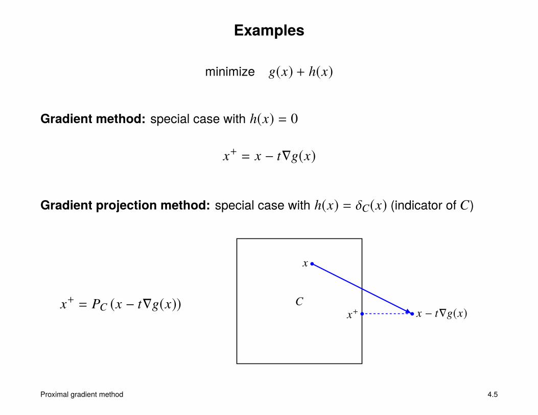
Examples

minimize g(x) + h(x)

Gradient method: special case with h(x) = 0

x+ = x − t∇g(x)

Gradient projection method: special case with h(x) = δC(x) (indicator of C)

x+ = PC (x − t∇g(x)) C

x

x − t∇g(x)x+


Examples

Soft-thresholding: special case with h(x) = ‖x‖1

x+ = proxth (x − t∇g(x))

where

(proxth(u))i =

ui − t ui ≥ t0 −t ≤ ui ≤ tui + t ui ≤ −t ui

(proxth(u))i

t−t


Outline

• motivation




Proximal mapping

if h is convex and closed (has a closed epigraph), then

proxh(x) = argminu

(h(u) + 1

2‖u − x‖22

)exists and is unique for all x

• will be studied in more detail in one of the next lectures

• from optimality conditions of minimization in the definition:

u = proxh(x) ⇐⇒ x − u ∈ ∂h(u)⇐⇒ h(z) ≥ h(u) + (x − u)T(z − u) for all z


Projection on closed convex set

proximal mapping of indicator function δC is Euclidean projection on C

proxδC(x) = argmin

u∈C‖u − x‖22 = PC(x)

u = PC(x)m

(x − u)T(z − u) ≤ 0 ∀z ∈ C

C

x

u

we will see that proximal mappings have many properties of projections


Firm nonexpansiveness

proximal mappings are firmly nonexpansive (co-coercive with constant 1):

(proxh(x) − proxh(y))T(x − y) ≥ ‖proxh(x) − proxh(y)‖22

• follows from page 4.7: if u = proxh(x), v = proxh(y), then

x − u ∈ ∂h(u), y − v ∈ ∂h(v)

combining this with monotonicity of subdifferential (page 2.9) gives

(x − u − y + v)T(u − v) ≥ 0

• a weaker property is nonexpansiveness (Lipschitz continuity with constant 1): proxh(x) − proxh(y)

2 ≤ ‖x − y‖2

follows from firm nonexpansiveness and Cauchy–Schwarz inequality


Outline

• motivation




Assumptions

minimize f (x) = g(x) + h(x)

• h is closed and convex (so that proxth is well defined)

• g is differentiable with dom g = Rn, and L-smooth for the Euclidean norm, i.e.,

L2

xT x − g(x) is convex

• there exists a constant m ≥ 0 such that

g(x) − m2

xT x is convex

when m > 0 this is m-strong convexity for the Euclidean norm

• the optimal value f? is finite and attained at x? (not necessarily unique)


Implications of assumptions on g

Lower bound

• convexity of the the function g(x) − (m/2)xT x implies (page 1.19):

g(y) ≥ g(x) + ∇g(x)T(y − x) + m2‖y − x‖22 for all x, y (1)

• if m = 0, this means g is convex; if m > 0, strongly convex (lecture 1)

Upper bound

• convexity of the function (L/2)xT x − g(x) implies (page 1.12):

g(y) ≤ g(x) + ∇g(x)T(y − x) + L2‖y − x‖22 for all x, y (2)

• this is equivalent to Lipschitz continuity and co-coercivity of gradient (lecture 1)


Gradient map

Gt(x) = 1t(x − proxth(x − t∇g(x)))

Gt(x) is the negative “step” in the proximal gradient update

x+ = proxth (x − t∇g(x))= x − tGt(x)

• Gt(x) is not a gradient or subgradient of f = g + h

• from subgradient definition of prox-operator (page 4.7),

Gt(x) ∈ ∇g(x) + ∂h (x − tGt(x))

• Gt(x) = 0 if and only if x minimizes f (x) = g(x) + h(x)


Consequences of quadratic bounds on g

substitute y = x − tGt(x) in the bounds (1) and (2): for all t,

mt2

2‖Gt(x)‖22 ≤ g (x − tGt(x)) − g(x) + t∇g(x)TGt(x) ≤ Lt2

2‖Gt(x)‖22

• if 0 < t ≤ 1/L, then the upper bound implies

g(x − tGt(x)) ≤ g(x) − t∇g(x)TGt(x) + t2‖Gt(x)‖22 (3)

• if the inequality (3) is satisfied and tGt(x) , 0, then mt ≤ 1

• if the inequality (3) is satisfied, then for all z,

f (x − tGt(x)) ≤ f (z) + Gt(x)T(x − z) − t2‖Gt(x)‖22 −

m2‖x − z‖22 (4)

(proof on next page)


Proof of (4):

f (x − tGt(x))≤ g(x) − t∇g(x)TGt(x) + t

2‖Gt(x)‖22 + h(x − tGt(x))

≤ g(z) − ∇g(x)T(z − x) − m2‖z − x‖22 − t∇g(x)TGt(x) + t

2‖Gt(x)‖22

+ h(x − tGt(x))≤ g(z) − ∇g(x)T(z − x) − m

2‖z − x‖22 − t∇g(x)TGt(x) + t

2‖Gt(x)‖22

+ h(z) − (Gt(x) − ∇g(x))T(z − x + tGt(x))= g(z) + h(z) + Gt(x)T(x − z) − t

2‖Gt(x)‖22 −

m2‖x − z‖22

• in the first step we add h(x − tGt(x)) to both sides of the inequality (3)

• in the next step we use the lower bound on g(z) from (1)

• in step 3, we use Gt(x) − ∇g(x) ∈ ∂h(x − tGt(x)) (see page 4.12)


Progress in one iteration

for a step size t that satisfies the inequality (3), define

x+ = x − tGt(x)

• inequality (4) with z = x shows that the algorithm is a descent method:

f (x+) ≤ f (x) − t2‖Gt(x)‖22

• inequality (4) with z = x? shows that

f (x+) − f? ≤ Gt(x)T(x − x?) − t2‖Gt(x)‖22 −

m2‖x − x?‖22

=12t

( x − x? 2

2 − x − x? − tGt(x)

22

)− m

2‖x − x?‖22

=12t

((1 − mt)‖x − x?‖22 − ‖x+ − x?‖22

)(5)

≤ 12t

(‖x − x?‖22 − ‖x+ − x?‖22

)(6)


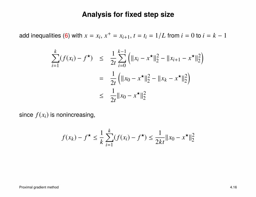
Analysis for fixed step size

add inequalities (6) with x = xi, x+ = xi+1, t = ti = 1/L from i = 0 to i = k − 1

k∑i=1( f (xi) − f?) ≤ 1

2t

k−1∑i=0

(‖xi − x?‖22 − ‖xi+1 − x?‖22

)=

12t

(‖x0 − x?‖22 − ‖xk − x?‖22

)≤ 1

2t‖x0 − x?‖22

since f (xi) is nonincreasing,

f (xk) − f? ≤ 1k

k∑i=1( f (xi) − f?) ≤ 1

2kt‖x0 − x?‖22


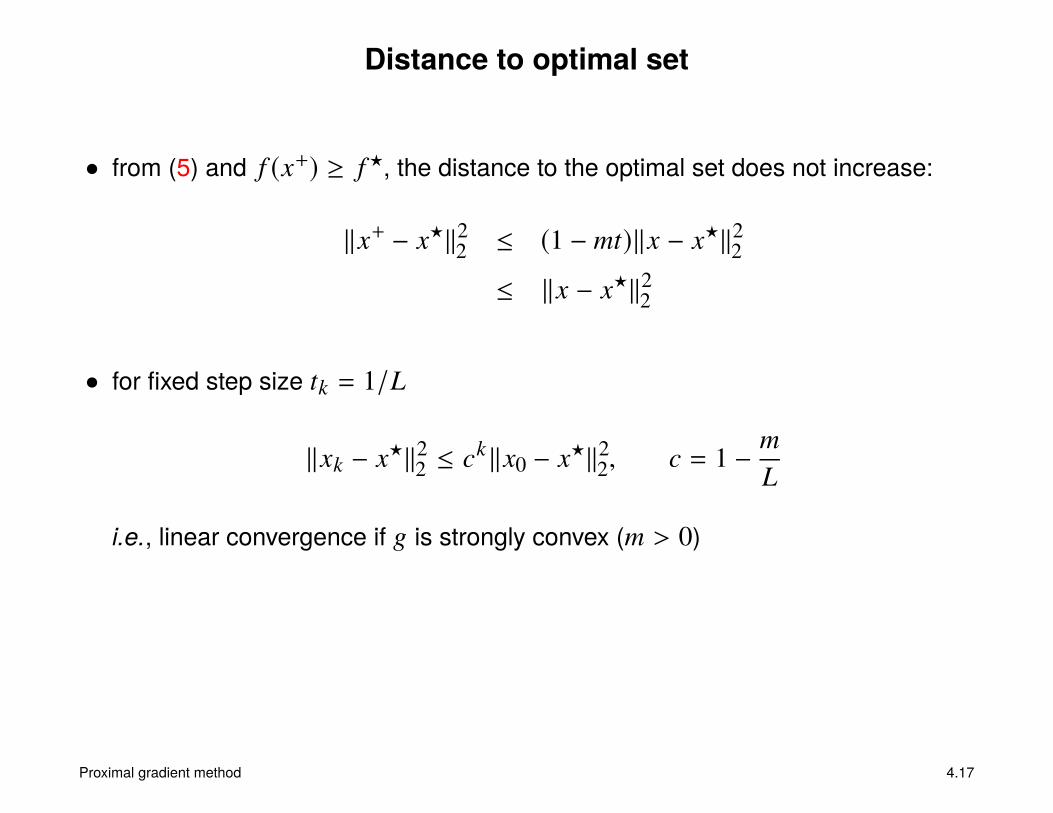
Distance to optimal set

• from (5) and f (x+) ≥ f?, the distance to the optimal set does not increase:

‖x+ − x?‖22 ≤ (1 − mt)‖x − x?‖22≤ ‖x − x?‖22

• for fixed step size tk = 1/L

‖xk − x?‖22 ≤ ck ‖x0 − x?‖22, c = 1 − mL

i.e., linear convergence if g is strongly convex (m > 0)


Example: quadratic program with box constraints

minimize (1/2)xT Ax + bT xsubject to 0 � x � 1

0 5 10 15 20 25 30 35 40 45 50

10−6

10−5

10−4

10−3

10−2

10−1

100

k

(f(x

k)−

f?)/

f?

n = 3000; fixed step size t = 1/λmax(A)Proximal gradient method 4.18

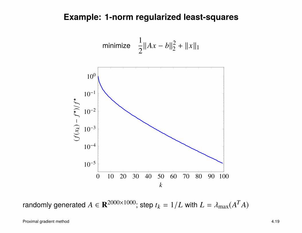
Example: 1-norm regularized least-squares

minimize12‖Ax − b‖22 + ‖x‖1

0 10 20 30 40 50 60 70 80 90 100

10−5

10−4

10−3

10−2

10−1

100

k

(f(x

k)−

f?)/

f?

randomly generated A ∈ R2000×1000; step tk = 1/L with L = λmax(AT A)Proximal gradient method 4.19

Outline

• introduction




Line search

• the analysis for fixed step size (page 4.13) starts with the inequality

g(x − tGt(x)) ≤ g(x) − t∇g(x)TGt(x) + t2‖Gt(x)‖22 (3)

this inequality is known to hold for 0 < t ≤ 1/L

• if L is not known, we can satisfy (3) by a backtracking line search:

start at some t := t̂ > 0 and backtrack (t := βt) until (3) holds

• step size t selected by the line search satisfies t ≥ tmin = min{t̂, β/L}

• requires one evaluation of g and proxth per line search iteration

several other types of line search work


Example

line search for gradient projection method

x+ = PC (x − t∇g(x)) = x − tGt(x)

C

x − t̂∇g(x) PC(x − t̂∇g(x))

x − βt̂∇g(x) PC(x − βt̂∇g(x))

x

backtrack until PC(x − t∇g(x)) satisfies the “sufficient decrease” inequality (3)


Analysis with line search

from page 4.15, if (3) holds in iteration i, then f (xi+1) < f (xi) and

ti( f (xi+1) − f?) ≤ 12

(‖xi − x?‖22 − ‖xi+1 − x?‖22

)• adding inequalities for i = 0 to i = k − 1 gives

(k−1∑i=0

ti) ( f (xk) − f?) ≤k−1∑i=0

ti( f (xi+1) − f?) ≤ 12‖x0 − x?‖22

first inequality holds because f (xi) is nonincreasing

• since ti ≥ tmin, we obtain a similar 1/k bound as for fixed step size

f (xk) − f? ≤ 12 ∑k−1

i=0 ti‖x0 − x?‖22 ≤

12ktmin

‖x0 − x?‖22


Distance to optimal set

from page 4.15, if (3) holds in iteration i, then

‖xi+1 − x?‖22 ≤ (1 − mti)‖xi − x?‖22≤ (1 − mtmin) ‖xi − x?‖22= c ‖xi − x?‖22

‖xk − x?‖22 ≤ ck ‖x0 − x?‖22

withc = 1 − mtmin = max{1 − βm

L, 1 − mt̂}

hence linear convergence if m > 0


Summary: proximal gradient method

• minimizes sums of differentiable and non-differentiable convex functions

f (x) = g(x) + h(x)

• useful when nondifferentiable term h is simple (has inexpensive prox-operator)

• convergence properties are similar to standard gradient method (h(x) = 0)

• less general but faster than subgradient method


References

• A. Beck, First-Order Methods in Optimization (2017), §10.4 and §10.6.

• A. Beck and M. Teboulle, A fast iterative shrinkage-thresholding algorithm forlinear inverse problems, SIAM Journal on Imaging Sciences (2009).

• A. Beck and M. Teboulle, Gradient-based algorithms with applications to signalrecovery, in: Y. Eldar and D. Palomar (Eds.), Convex Optimization in SignalProcessing and Communications (2009).

• Yu. Nesterov, Lectures on Convex Optimization (2018), §2.2.3–2.2.4.

• B. T. Polyak, Introduction to Optimization (1987), §7.2.1.


https://doi.org/10.1137/1.9781611974997

https://doi.org/10.1007/978-3-319-91578-4

L.Vandenberghe ECE236C(Spring2019) 4.Proximalgradientmethodvandenbe/236C/lectures/proxgrad.pdf ·...

Documents

Transcript of L.Vandenberghe ECE236C(Spring2019) 4.Proximalgradientmethodvandenbe/236C/lectures/proxgrad.pdf ·...