|

Lund University

Lund University, with eight faculties and a number of research centres and specialized institutes, is the largest establishment for research and higher education in Scandinavia. The main part of the University is situated in the small city of Lund which has about 112 000 inhabitants. A number of departments for research and education are, however, located in Malmö. Lund University was founded in 1666 and has today a total staff of 6 000 employees and 47 000 students attending 280 degree programmes and 2 300 subject courses offered by 63 departments.

Master Programme in Energy-efficient and Environmental Building Design

This international programme provides knowledge, skills and competencies within the area of energy-efficient and environmental building design in cold climates. The goal is to train highly skilled professionals, who will significantly contribute to and influence the design, building or renovation of energy-efficient buildings, taking into consideration the architecture and environment, the inhabitants’ behaviour and needs, their health and comfort as well as the overall economy.

The degree project is the final part of the master programme leading to a Master of Science (120 credits) in Energy-efficient and Environmental Buildings.

Examiner: Maria Wall Supervisor: Marie-Claude Dubois

Keywords: light pipe; tubular daylight guiding systems; daylighting; hollow light guides; tubular skylight; forward raytracing simulation; building energy; sustainable technology; interior illuminance; raytracing; TracePro; mirrored light pipe; light pipe aspect ratio; solar elevation; roof tilt; specular reflectance; light pipe reflectance; light pipe design.

Thesis: EEBD-14/02

1

Abstract Daylighting usage is an effective way to reduce energy consumption in buildings.

Light pipes are effective devices used to bring daylight to the back of deep plan buildings. However, there is a lack of reliable methods to predict their performance due to their optical complexity. This paper evaluates the suitability of a forward raytracing tool to predict light pipes performance. Simulation results are compared to illuminance measurements done in two pig stables equipped with light pipes near Lund, in Sweden. The results for overcast skies show an acceptable level of accuracy, given the high levels of uncertainty (discrepancies were lower than 22% for 95% of the cases assessed). The results with direct sunlight show similar trends and values at low solar altitudes for measurements and simulation results. However, as the solar altitude is raised the discrepancies increase. This is caused by a certain overestimation of direct sunlight and the lack of optical characterization of the light-bending properties of the dome collectors in some of the light pipes.

In the second part of the thesis, the forward raytracing tool is used to achieve a parametric study of some key design parameters of simple light pipes, including location, aspect ratio, pipe reflectance and roof tilt orientation. The results demonstrate the importance of location and cloud coverage for the light pipe performance. They suggest that simple light pipes are best suited for mid or low latitudes with prevalence of clear skies, although the use of optical redirecting systems (ORS) could improve the performance for higher latitudes. Aspect ratio and specular reflectance of the pipe were found to be the most important design parameters of light pipes.

2

Acknowledgements I would like to thank Marie-Claude Dubois, my research supervisor, for her

professional guidance, enthusiastic encouragement and valuable and useful critiques of this research project. Special thanks should be given to Hans von Wachenfelt and Niko Gentile for their valuable support; with the collection of onsite measurements. I also thank Maria Wall, for her advice and assistance in keeping my progress on schedule. My gratitude is also extended to Jouri Kanters, Henrik Davidsson, Ricardo Bernardo and Eja Pederson for their help and guidance in completing some of the tasks included in this project. Their willingness to give their time so generously has been very much appreciated. I give special thanks to the Eliasson Foundation for funding me during my master studies. I Lastly, I acknowledge the help and moral support from my classmates and friends Thorunn Arnardottir and Ariane Hartmann.

3

Table of Contents Abstract ................................................................................................................................... 1

Acknowledgements ................................................................................................................. 2

Definitions/Acronyms ............................................................................................................. 5

1 Introduction ..................................................................................................................... 8

1.1 Background and problem motivation .................................................................... 10

1.2 Overall aims ........................................................................................................... 19

1.3 Scope and limitations............................................................................................. 20

1.3.1 Evaluation of the simulation method ................................................................. 20

1.3.2 Parametric study ................................................................................................ 20

2 Methodology ................................................................................................................. 22

2.1 Presentation of the ‘pig stables’ case study ........................................................... 23

2.2 Field measurements ............................................................................................... 32

2.3 Selection of raytracing method .............................................................................. 35

2.4 Description of the simulation method utilized ....................................................... 38

2.5 Sources of error ..................................................................................................... 43

A. Variability of the measurements ....................................................................... 43

B. Dirtiness deposition on the indoor sensors ....................................................... 44 C. Daylight on/off sensor....................................................................................... 43

D. Inaccuracies in the virtual model ...................................................................... 43

E. Optical characterization of the light pipes......................................................... 43

F. Location of the ports.......................................................................................... 43

G. Use of generic sky models ................................................................................ 43

2.6 Parametric study .................................................................................................... 52

3 Results ........................................................................................................................... 55

3.1 Evaluation of the simulation method ..................................................................... 55

3.2 Parametric study results ......................................................................................... 63

4 Discussion ..................................................................................................................... 73

4.1 Evaluation of the simulation method ..................................................................... 73

4.2 Parametric study .................................................................................................... 77

4.2.1 Solar altitude ...................................................................................................... 77

4.2.2 Aspect ratio ........................................................................................................ 78

4

4.2.3 Light pipe illuminance ....................................................................................... 79

4.2.4 Roof tilt .............................................................................................................. 79

5 Conclusions ................................................................................................................... 81

5.1 Forward raytracing as simulation method for light pipes ...................................... 81

5.2 Guidelines for light pipe design ............................................................................. 82

5.3 Future research ...................................................................................................... 83

6 References ..................................................................................................................... 84

Appendix A: Simulation methodology evaluation detailed results ....................................... 88

Appendix B: calculation of the average absolute deviation (AAD) of the measurements .... 95

Appendix C: Luminance distribution assessment of the parametric study ............................ 97

5

Definitions/Acronyms

The list below gives the definition of some technical concepts and specific terms included in this paper:

Light absorptance: surface optical property that expresses the fraction of the incident light that is absorbed in a material.

Aspect ratio: applied to light pipes, the aspect ratio is the diameter of the pipe divided by the total length from collector to diffuser and expressed as a ratio. It is a crucial factor in light pipe performance.

Average absolute deviation (AAD): statistical value used to express how a set of data differs from its mean value.

Bi-directional scattering distribution function (BSDF): is an advanced and detailed optical characterization of a surface. It defines the direction and intensity of the outgoing light rays (reflected or transmitted) as a function of sets of incident rays at given incident angles on a certain point in the surface.

Clear sky: at least 7/8 of the sky must be uncovered for the sky to be considered clear, and the covered patch of the sky must not cover the sun or be seen from the interior.

Commission Internationale de l’Éclairage (CIE): In English, International Commission on Illumination. According to their website (www.cie.co.at), the CIE is an organization devoted to worldwide cooperation and the exchange of information on all matters relating to the science and art of light and lighting, color and vision, photobiology and image technology.

Core daylighting: techniques aiming to bring natural light to indoor spaces located far from the building exterior envelope.

Daylight factor (DF): used to express indoor daylight levels. It is a ratio that defines the indoor horizontal illuminance at a given point at work plane height compared to the simultaneous unshaded outdoor horizontal global illuminance under a CIE overcast sky.

Daylight on/off system: control system that turns the lights on when daylight does not reach a certain threshold and turns them off when the threshold is exceeded.

Diffuse light reflectance: portion of the reflectance that is diffuse, not specular.

Fresnel lens: specially designed lens that allow relatively short focal length and high aperture but requires less volume and material than a conventional lens of similar characteristics.

Global horizontal illuminance (GHI): total outdoor illuminance measured on a horizontal plane pointing upwards in an unobstructed environment.

Goniophotometry: technique that measures the angular distribution of scattered light - either transmitted or reflected - as a function of the incident angle.

Illuminance (E): photometric property that defines the luminous flux incident on a surface, per unit area. It is usually measured in lux (lx).

6

Intermediate sky: sky characterized by a mixture of sun and clouds i.e., sky with cloud coverage higher than clear skies and lower than overcast skies.

International Energy Agency (IEA): established in 1974 within the framework of the Organization for Economic Co-operation and Development (OECD) to implement an international energy program. A basic aim of the IEA is to foster co-operation among the twenty-eight IEA participating countries and to increase energy security through energy conservation, development of alternative energy sources and energy research, development and demonstration (RD&D).

Light loss factor (LLF): proportion of daylight lost in a light pipe for a given solar position and sky type. It is expressed as the amount of light that does not reach the interior space in relation to the total incident light on the collector.

Light transmission factor (LTF): denotes the percentage of light that goes through a light pipe for a given solar position and sky type. It is expressed as the proportion of daylight emitted by the diffuser in relation to the total incident light on the collector.

Mirrored light pipe (MLP): highly reflective pipe, usually cylindrical, used in light pipes to transport daylight from the collector to the diffuser.

National Fenestration Rating Council (NFRC) American entity responsible for determining standards and ratings for fenestration products in terms of energy performance, wind and moisture resistance, daylighting, etc.

Optical redirecting systems (ORS): innovative systems that deflect light to focus it where most needed, spread it or avoid glare. Some samples of ORS in light pipes are: special dome collectors designed to redirect low solar angles into the pipe, special reflectors in the collector or diffusers.

Overcast sky: sky entirely or mostly covered by clouds.

Light reflectance: optical property of surfaces that expresses the fraction of the incident light that is reflected from the surface.

Light refraction: alteration of the direction of light propagation produced at the boundary between two media with different refraction index.

Raytracing: it is a technique for generating an image by tracing the path of light through pixels in an image plane and simulating the effects of its encounters with virtual objects.

Light scatter: random reflection of light rays from their straight path when propagating though a medium due to irregularities on its surface.

Sensor dirt factor (SDF): factor used in this research project to consider the effect of dirt deposition on the sensors.

Sky clearness index (Kt): factor that expresses the proportion of sky covered by clouds at a given location and time. It ranges from 0 (total absence of clouds) to 1 (completely covered). Clear skies are usually defined by Kt lower than 0.18 and overcast skies by Kt higher than 0.7. Values in between these two figures correspond to intermediate skies.

7

Solar altitude: angle that defines the position of the sun in the sky in reference to its closest point of horizon.

Specular light reflectance: optical property of surfaces that expresses the fraction of the incident light that is reflected at an angle with the surface normal equal to the angle of the incident light with respect to the normal.

Light transmittance: optical property of materials that expresses the fraction of the incident light that passes through it.

Tubular daylight guiding systems (TDGS): more commonly called light pipes, these innovative systems are used to bring daylight though the roof into indoor spaces distant from facades.

8

1 Introduction This master thesis is part of larger project on the potential of light pipes to reduce

electric light dependency in pig stables. This larger project, called Can new technologies reduce the use of electricity and improve daylight in pig houses?, is currently achieved by Alnarp University in collaboration with Lund University’s Division of Energy and Building Design. In this larger project, indoor illuminance levels are measured in two pig stables equipped with light pipes to assess the daylight levels attained. An automatic on/off daylight switch is installed to save electricity when there is sufficient daylight. Electric light consumption is monitored to calculate yearly electricity savings.

The first part of this master thesis compares the illuminance values measured in the pig stables with the values obtained with forward raytracing simulations. The main goal of this part is to assess the accuracy of the forward raytracing simulation method applied to light pipes. The results of this comparison indicate that the forward raytracing program predicts correctly illuminance levels under overcast skies but overpredicts them under clear skies. A continuation of this research project will be undertaken after the completion of this thesis to solve this problem and find a way to apply forward raytracing to climate based annual simulations. This will permit the estimation of annual electricity savings obtained with the use of light pipes.

The second part of this thesis uses the forward raytracing method to carry out a parametric study concerning the relative importance of key configuration parameters for the performance of simple light pipes. Four parameters are assessed: solar elevation, aspect ratio, reflectance, and roof tilt orientation. The results indicate that sky clearness, solar elevation and specular reflectance of the pipe are the most important parameters affecting light pipe performance.

Figure 1.1 summarizes the method used in this thesis.

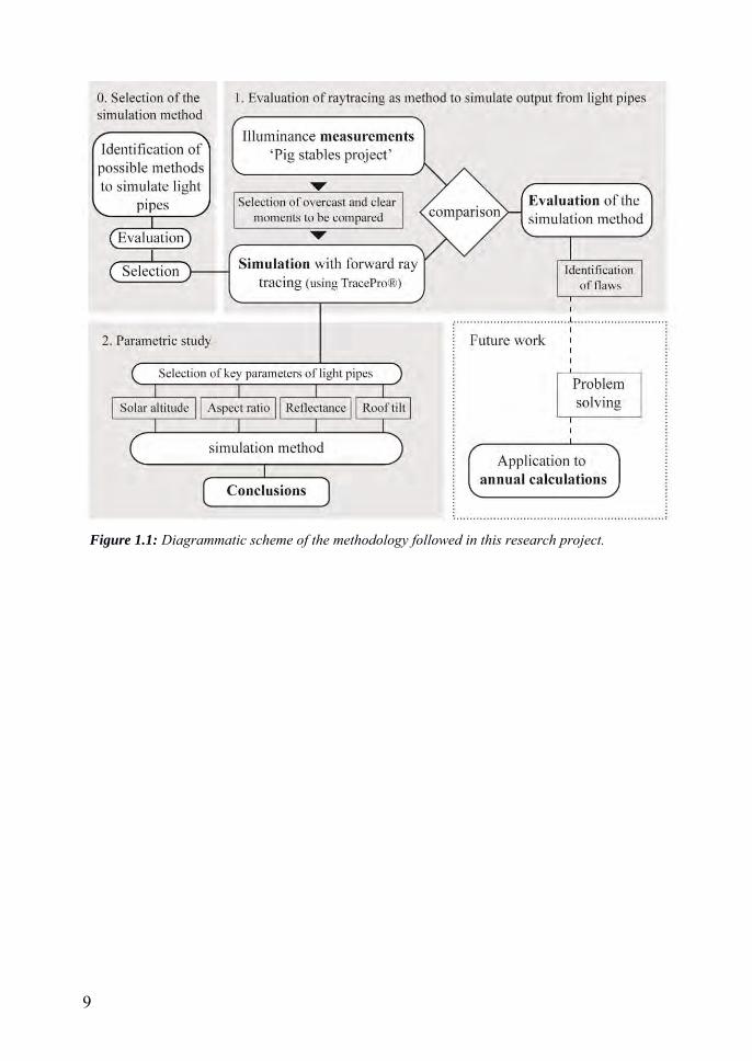
9

Figure 1.1: Diagrammatic scheme of the methodology followed in this research project.

10

1.1 Background and problem motivation

Light pipes have a great potential to reduce of electricity use in buildings. However, there is a lack of reliable simulation methods to predict their performance. Intensive energy use implies negative environmental impacts. Electric lighting is directly responsible for 7% of the total CO2 global emissions and 19% of the world’s electricity consumption (Energy Information Administration, 2007). Daylight usage is a cost efficient strategy to reduce electric lighting consumption. The use of daylight is also proven to increase occupants’ sociability, well-being productivity and health (Dehoff, 2002) (Harteb Puleo & Leslie, 1991) (Figueiro, 2002). Rear spaces in deep plan buildings usually have scarce access to daylight. Light pipes are an effective passive way to bring daylight to these spaces and are ideal for retrofit situations. They are composed of 3 parts: collector, mirrored light pipe (MLP) and diffuser. They can bring daylight to deep spaces without producing glare or increasing the cooling needs. They are complex systems usually fitted with Optical Redirecting Systems (ORS), which makes their light output difficult to predict. Numerical methods, based on raytracing computational software, are a promising method to simulate light pipes. This paper evaluates the accuracy of a commercial forward raytracer to simulate the output from light pipes by comparing the simulation results to illuminance measurements in two pig stables near Lund, (Sweden).

The importance of reducing electricity consumption

About 40% of the world’s primary energy is devoted to produce electricity (International Energy Agency, 2006). A significant abatement of the global electricity consumption is essential to tackle the reduction of environmental impacts.

Environmental impacts are an issue of major concern worldwide. The intensive release of greenhouse gases (GHG), especially CO2, has already produced a global warming of half a degree Celsius and is expected to increase an additional half a degree in the next few decades (Stern, 2007). Energy use is responsible for the great majority of GHG emissions (International Energy Agency, 2006). In the member countries of the European Union about half of the energy consumed is imported. This energy dependence from other countries can lead to diplomatic tensions and security issues. For these reasons the EU has the target of reducing its GHG emissions by 20% and improving energy efficiency by another 20% by year 2020.

Electricity is a large and fast growing cause of GHG emissions. The environmental impact of that electricity consumption is equivalent to about 70% of the GHG emissions of light passenger vehicles globally, i.e 1,900 Mt of CO2 per year (International Energy Agency, 2006). Foreseeably, the distribution of that electricity consumption for lighting presents an uneven distribution from traditionally developed to developing countries. However, the latter are rapidly urbanising and, by 2030, most predictions indicate a global demand increase of 80% for electric lighting (Energy Information Administration, 2007) mainly due to the growth of those developing countries.

Electricity consumption is directly responsible for a large share of the world primary energy production. Primary energy can be defined as the energy that has not been subjected to transformations. The environmental impacts of electricity consumption depend – to a large extent – on the way that electricity is produced. In Europe, as an average, 2.5 kWh of

11

primary energy are required to produce 1 kWh of electricity (Eurostat, 2009). This offset is caused by the fact that it takes into account the energy losses due to the generation and delivery processes. For this reason, although electricity consumption was ‘only’ 11.8% of the global energy consumption in 2005 (International Energy Agency, 2006), the actual primary energy used to produce that electricity has risen to 40% (Hore-Lacy, 2003).

The abatement potential of electric light

Lighting is a major and fast growing electricity consuming sector and GHG source. About 99% of the light consumed globally is powered by electricity (International Energy Agency, 2006). Almost a fifth of the electricity produced globally is consumed by the lighting sector (International Energy Agency, 2006). In view of this, lighting is a key sector to improve in terms of energy-efficiency in order to reduce global electricity demand.

Electric light consumption is expected to continue growing in the decades to come, mainly due to urbanization trends occurring in developing countries. In the IEA countries, which mostly include industrialized countries; electric light demand grew only by 1.8% in the last decade (International Energy Agency, 2006). This might be a sign of saturation in the traditionally industrialized countries. On the other hand, developing countries are rapidly increasing their lighting demand. A quick urbanization process, demographic growth and the rise of the illuminance levels are leading causes of this increase (International Energy Agency, 2006).

Electric light is mostly consumed in buildings. In Europe, buildings are responsible for about 40% of the total energy consumption (International Energy Agency, 2006). Most of that energy is devoted to lighting: 50% in office buildings, 20-30% in hospitals, 15% in factories, 10-15% in schools and 10% in dwellings (Energy Information Administration, 2007). Another indirect impact of lighting is that it produces heat as a side effect, which increases cooling loads. That additional heat also contributes to reduce the heating demand in cold climates. However, heating systems produce heat more efficiently than lighting, and at the right place (e.g. near the feet). It is in fact more beneficial, in terms of thermal comfort, to produce heat with a proper heating system instead of lighting.

Traditionally, the efforts to make buildings more energy efficient were focused in the heating and cooling needs, leaving electric lighting as a secondary issue. Even countries with strong interest and long tradition in environmental building design such as Sweden have failed to invest in lighting. Sweden has made important achievements in energy efficiency by promoting adequate policies such as passive house renovations or stricter regulations. However, most of this was oriented to reducing heating loads and/or providing greener heat sources. Electricity bills and environmental impacts are now dominated by lighting which still has a large potential of optimization. The commercial building sector in Sweden has especially been characterized by reduction in heating demand over the last decades but a great increase in electricity demand. Today an ordinary office building uses half of its energy as electricity (Flodberg, 2013).

Besides being an energy consuming sector, electric lighting is also quite costly. Its total annual cost represented in 2006 about 1% of the global GDP, i.e. USD 360 billion; electricity use being directly responsible for two thirds of that value (International Energy Agency, 2006).

12

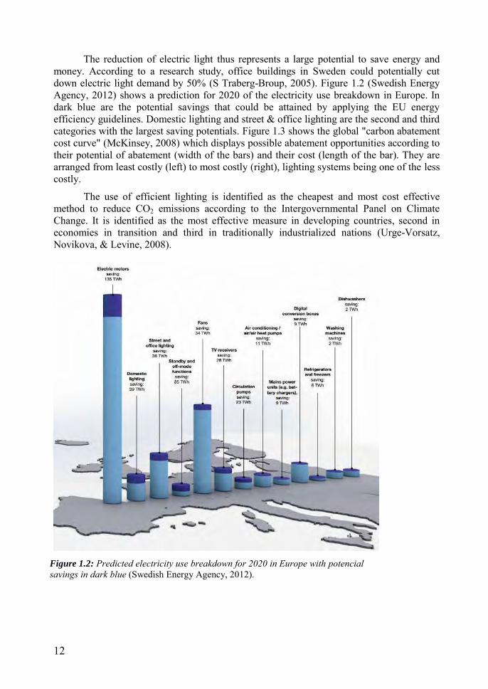
The reduction of electric light thus represents a large potential to save energy and money. According to a research study, office buildings in Sweden could potentially cut down electric light demand by 50% (S Traberg-Broup, 2005). Figure 1.2 (Swedish Energy Agency, 2012) shows a prediction for 2020 of the electricity use breakdown in Europe. In dark blue are the potential savings that could be attained by applying the EU energy efficiency guidelines. Domestic lighting and street & office lighting are the second and third categories with the largest saving potentials. Figure 1.3 shows the global "carbon abatement cost curve" (McKinsey, 2008) which displays possible abatement opportunities according to their potential of abatement (width of the bars) and their cost (length of the bar). They are arranged from least costly (left) to most costly (right), lighting systems being one of the less costly.

The use of efficient lighting is identified as the cheapest and most cost effective method to reduce CO2 emissions according to the Intergovernmental Panel on Climate Change. It is identified as the most effective measure in developing countries, second in economies in transition and third in traditionally industrialized nations (Urge-Vorsatz, Novikova, & Levine, 2008).

Figure 1.2: Predicted electricity use breakdown for 2020 in Europe with potencial savings in dark blue (Swedish Energy Agency, 2012).

13

Figure 1.3: Carbon abatement cost curve (McKinsey, 2008).

Daylight usage

One of the most obvious way to reduce electric light consumption is the optimization of the daylight usage. The biggest challenge of daylighting is to reach deep spaces far from the façades. This is called core daylighting. Light pipes are one of the most common core daylighting systems.

Daylight usage optimization a cost efficient strategy to reduce electric lighting needs and the most user friendly. It was ranked among the six strategies with significant potential identified in 2006 by the IAE (International Energy Agency, 2006). Daylight is free and requires no energy to be produced. Furthermore, daylight use can contribute to reduce not only total energy needs but also peak energy loads since it is most available right during working hours.

Other benefits of daylight are listed below:

- It is much preferred to electric light by building users (Dehoff, 2002). - It improves the mood and the vigilance in humans as it is directly linked to the

circadian cycle. - It has similar effects for many animal species (Ashkenazy, Einat, & Kronfeld-

Schor, 2009). - Its continuous spectral distribution provides optimal color rendering. - Daylight – especially skylight – has a better luminous efficacy than most electric

light sources. This means it has less associated heat. - It enhances the motivation and productivity of the workers (Harteb Puleo &

Leslie, 1991). - Increases significantly sales in retail spaces (Heschong Mahone Group, 2003).

14

Daylight also has some drawbacks and limitations. It can produce inconveniences such as glare or high cooling loads if not properly handled. Some conventional strategies linked to daylight are: good shading device design; appropriate window size, position and orientation; increase of the reflectance of the interior surfaces and reduction of partition height.

Windows are the most common daylighting system but they are limited to serve peripheral area of buildings. The great majority of buildings uses windows as the main daylighting system. Windows allow visual connections with the outdoor context and are good at lighting vertical surfaces, which makes spaces look brighter. However, they are usually insufficient to bring daylight to the rear of deep building plans. In spaces with side daylighting (windows), the daylight levels decrease rapidly with the distance from the windows. The floor area lit by windows is limited to about 1.5 times the window’s head height (IESNA, 1999). As a consequence, additional lighting, using electric lighting or core daylighting systems is required to keep suitable light levels and to provide an even light distribution within deep spaces.

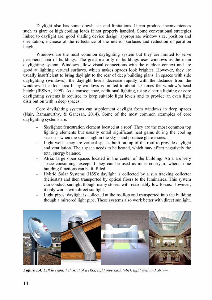
Core daylighting systems can supplement daylight from windows in deep spaces (Nair, Ramamurthy, & Ganesan, 2014). Some of the most common examples of core daylighting systems are:

- Skylights: fenestration element located at a roof. They are the most common top lighting elements but usually entail significant heat gains during the cooling season – when the sun is high in the sky – and produce glare issues.

- Light wells: they are vertical spaces built on top of the roof to provide daylight and ventilation. Their space needs to be heated, which may affect negatively the total energy balance.

- Atria: large open spaces located in the center of the building. Atria are very space consuming, except if they can be used as inner courtyard where some building functions can be fulfilled.

- Hybrid Solar Systems (HSS): daylight is collected by a sun tracking collector (heliostat) and then transported by optical fibers to the luminaires. This system can conduct sunlight though many stories with reasonably low losses. However, it only works with direct sunlight.

- Light pipes: daylight is collected at the rooftop and transported into the building though a mirrored light pipe. These systems also work better with direct sunlight.

Figure 1.4: Left to right: heliostat of a HSS, light pipe (Solatube), light well and atrium.

15

Light pipe

Light pipes can bring daylight to deep spaces without producing glare or increasing the cooling needs. However, their performance is very limited under overcast skies and their use is usually restricted to the two top floors. They are usually fitted with complex ORS such as light redirecting collectors, reflectors or light diffusers, which makes their light output difficult to predict. This lack of predictability hinders their widespread use and effective implementation.

Light pipes or TDGS are vertical, roof-mounted systems that use MLP and sophisticated optical devices to bring daylight into deep interior spaces. Although light pipes cannot replace traditional windows, they can be used as the supplementary daylight system in deeper rooms and therefore reduce electric light dependency (Mohelnikova, 2009). Their use achieves energy savings and provides a natural spectrum and dynamic variations of daylight. Light pipes are, after skylights, the most common roof-mounted daylighting system (Nilsson, 2012). Compared to skylights, light pipes present the advantage of effectively capturing direct beam radiation from the sun while avoiding excessive heat gains and glare patches. Light pipes have the advantage of being ideal in retrofit situations, an issue which is very relevant since most building that existing today will still be there in 2050.

Their main drawback is that their performance is much affected by sky-clearness (Zhang & Muneer, 2000). They are efficient in capturing direct sunlight but produce much lower light levels under overcast sky conditions (Mohelnikova, 2009). They are thus better suited for climates with abundance of clear skies (Nilsson, 2012). This is a matter of great concern in Sweden where the climate presents a very high proportion of overcast skies (Figure 1.5) (The European Database of Daylight and Solar Radiation). It should be noted that the proportion of direct/diffuse radiation in Sweden is only about 1/1 (Khellsson, 2002), which is quite low compared to most countries. In an experiment run in Hong Kong with light pipes (Danny, Ernest, Cheung, & Tam, 2010) sky clearness indexes (Kt) below 0.18 gave out illuminance levels between 8 and 55 lx indoors, while a sky clearness index above 0.7 produced in all cases an interior illuminance above 200 lx.

16

Light pipe technology cannot be used in all types of spaces. Their use is usually recommended for top floors. They could also serve the second highest story if a poorer performance is accepted. One of the main light pipe manufacturers is called Solatube. Solatube’s website states (Solatube International, Inc.) that the space served by the light pipes should not be further than 9 meters from the rooftop. Their use is therefore very suitable for large one-story buildings like industrial units, sheds or livestock houses. These flat building typologies can hardly be properly lit relying only on windows and generally top daylighting or electric lights are required.

In the last few decades, light pipes have firmly set foot in many markets around the globe. However, there is still a considerable lack of know-how, standardization or rating systems for light pipes according to the American National Fenestration Rating Council (NFRC) (National Fenestration Rating Council, 2008). The uncertainty associated with their use needs to be reduced by means of accurate performance prediction methods. The availability of such methods would promote their wider acceptance and use (Dutton & Shao, 2007).

Figure 1.5: Frequency of sunny skies in Europe (The European Database of Daylight and Solar Radiation). In Scandinavian countries they represent only 10-30% of the annual sky distribution.

17

Simulation methodologies for light pipes

Light pipes are usually equipped with complex ORS, which makes it difficult to estimate their light output. Scaled physical models, empirical methods and analytical methods are limited in terms of accuracy, applicability to various sky conditions and adaptability to different light pipe models and configurations. Numerical methods, based on raytracing computational software, are a much more promising method to predict the performance of light pipes.

Light pipes are complex daylighting systems and as such it is hard to estimate their performance. Daylight has to go through many bounces inside a light pipe before reaching the interior space. Moreover, they are often equipped with several sophisticated Optical Redirecting Systems (ORS). Due to that complexity, it is difficult to create a simple method to predict their light output or estimate the number of light pipes required to comply with a certain daylight requirement. Overcoming these limitations will help to guide architects and light designers at the early stages of a project.

One way to simulate performance of daylighting systems is by building scale models. However, this is usually expensive, laborious and unreliable as it is difficult to accurately reproduce the building and its light pipes. Scale models tend to overestimate the daylight performance; errors of 30-50% have been reported (Thanachareonkit, Scartezzini, & Andersen, 2005).

Spencer Dutton and Li Shao differentiated in 2013 (Dutton & Shao, 2007) three types of methods to assess light pipe performance: empirical, analytical and numerical methods.

- A. Empirical methods: are based on experimental results but their application is limited to the specific conditions in which the experiment was conducted. They provide a series of formulas to calculate light output in determined conditions. Its applicability to other locations or climates is thus very limited.

- B. Analytical methods: are based on a purely mathematical approach which is also limited to respond to the great variability of sky conditions and the geometrical complexity of light pipes.

Kómar and Darula (Kómar & Darula, 2011) presented theoretical calculations of the LTF of light pipes using an analytical prediction method compared with measurement results obtained under an artificial sky. The main aim of their work was to offer a method to determine MLP reflectance and mathematically prove that light guide transmission efficiency is different for various standardized overcast sky types. They concluded that theories with constant inner reflectance of the pipe are not sufficient for accurate prediction of light guide transmission efficiency and proved the importance of accurately simulating the sky luminance distribution to predict the light pipe performance.

Other examples of analytical prediction methods for light pipes were presented by (Jenkins & Muneer, 2003), (Jenkins, Munner, & Kubie, 2005), (Mohelníková & Vajkay, 2009) and (Swift, Lawlor, Smith, & Gentle, 2008). These methods will not be developed here as this project is focused on numerical methods.

18

- C. Numerical methods: are based on computer simulations using raytracing software. It is so far the best method to predict light pipe performance, because of its accuracy, adaptability and inclusion of different variables (sky type, sun position, system geometry, ect.) (Kohler, 2010) (Dutton & Shao, 2007). However, its implementation requires a good knowledge of raytracing software. So far, there are few examples of light pipes simulation using raytracing software.

Kocifaj, Darula and Kittler developed HOLIGILM in 2007 (Kocifaj, Darula, & Kittler, 2007) which is a raytracing based program to predict light pipe performance. However, this software is quite limited in its possibilities to modify the geometry of the room and the light pipes and simulate ORS. Furthermore, no evaluation of the accuracy of this method has been presented so far.

Only one article comparing real light measurements with raytracing simulations with light pipes was found. In it, Farrell et al. (Farrel, Norton, & Kennedy, 2004) compared the daylight factors measured at the base of two light pipes to simulation results. They used the simulation program Radiance and combined the two variants of raytracing (forward and backward raytracing). Their results show high discrepancies of 40-75%.

19

1.2 Overall aims

1.2.1 Evaluate forward raytracing as a suitable prediction tool for light pipes

Light pipes are complex optical systems, which is why it is hard to estimate their light output. The lack of performance predictability methods hinders the widespread use of light pipes. It is necessary to allow an accurate assessment of the number and arrangement of light pipes in order to reach specific light levels at given situations. The lack of simulation tools yields a situation where light pipes’ benefits cannot be quantified and considered in environmental building rating systems, such as LEED or BREEAM.

This thesis thus pursues the aim of evaluating a forward raytracing tool for light pipes and compares the output to illuminance measurements in a full-scale pig stable located near Lund, Sweden.

1.2.2 Analyze the effect on performance of some key parameters of light pipe configuration

Architects and light designers require a basic knowledge of the principles of light pipes and their key design factors in order to be able to use them correctly. The raytracing tool is used to carry out a parametric study that assesses the influence of some key parameters of the light pipe design. This comparison aims to provide guidelines to architects and designers, which will result in a better understanding of the consequences of design choices concerning light pipes. The effect of light pipe aspect ratio and reflectance, roof tilt and solar altitude is thus investigated.

20

1.3 Scope and limitations

1.3.1 Evaluation of the simulation method

Two identical pig stables are assessed. Each of the stables is equipped with a different type of light pipe. Both types are included in this study to facilitate the extrapolation of the results to other cases. Both flat (Velux) and dome (Solatube) collectors are studied. Both light pipes with a straight (Solatube) and a bent (Velux) pipe are studied.

This project has at least four limitations described in the following:

All components in the Velux light pipes were correctly characterized by the data provided by the manufacturer, including goniophotometric information for the diffuser. However, in the case of the other manufacturer (Solatube) simulations do not integrate the special optical data (goniophotometric data) required for the complex components of the Solatube light pipe (dome collector and diffuser). This is due to the refusal of the manufacturing company to provide this data and the lack of means to develop own goniophotometric measurements.

In raytracing simulations the rays can be traced from the source to the point of view (forward raytracing) or from the point of view to the source (backward raytracing). In this forward raytracing was used. The other variant – backward raytracing – is excluded from the scope of this research project. This decision is based on the limitations of that method to accurately account for direct sunlight. These limitations and possible workarounds to it are described further on in this text.

Skies are divided in three groups according to their cloud coverage: overcast, intermediate and clear. Intermediate skies were not tested due to their great variability and complexity. The study covers only clear and overcast skies. These types of sky present a higher degree of homogeneity and predictability, which makes them more suitable for comparison with computer simulations. However, as they are complex elements subject to constant change, their representation still entails an intrinsic error source.

Finally, this study only covers solar altitudes below 28° due to the availability of measurements from December to the beginning of March. It would have been desirable to have data for the summer months as well in order to be able to verify the correspondence of the simulation results with the measurements for higher solar altitudes.

1.3.2 Parametric study

The parametric study was based on prevailing conditions in the context of the EU. Therefore, the highest solar altitude considered is 76°, corresponding to the highest solar altitude in Malaga (Southern Spain).

The light pipes simulated in this parametric study are very simple: they all have a flat collector and a straight pipe. It should be noted that this parametric study might not be relevant for systems using innovative dome collectors or more complex pipe geometries.

The effect varying collector and diffuser light transmittance on the LFT was overlooked as it is obviously directly proportional. Other parameters that could have been

21

included are: pipe shape, pipe bends, pipe tilt, use of reflectors, collector type and diffuser type.

The base case location for all the simulations was Malmö, except evidently for the parametric study on location. Therefore, the applicability of some of the simulation results is restricted to Northern European latitudes, i.e. 50°-60°, although in most other cases the trends should be similar to the ones showed in this study.

The range of reflectance assessed was limited to the common values used in MLP, i.e. 96% to 99.7%. Lower values are usually considered too low for this purpose and higher values would be unrealistic.

In the section on roof tilt only horizontal and 30° roofs are analyzed for different orientations when relevant. As so, the evolution of the light output for different tilt angles was not included within the scope of this study.

22

2 Methodology This section is organized according to the following six subsections. Subsections 1 to

5 describe the methodology followed to evaluate the suitability of forward raytracing as a simulation method for light pipes using the case study of the pig stables. Subsection 6 presents the method relating to the parametric study.

23

2.1 Presentation of the ‘pig stables’ case study

This subsection presents a description of the two stables used in this study as a case study for the evaluation of forward raytracing to predict the performance of light pipes. Two identical stables near Lund were fitted with 4 light pipes each. Light pipes in stable 1 (Velux Sun Tunnel®) have a bent and a flat collector while as the ones in Stable 2 (Solatube Brighten Up®) are straight and have an innovative dome collector equipped with a reflector to redirect low-angle sunlight. Two illuminance sensors were placed in each of the stables: one right below a light pipe and another one between two light pipes. A fifth sensor was located outdoors to measure the global horizontal illuminance. The geometry and optical properties of the stable were measured and modelled in TracePro. The light pipes were characterized with information provided by the manufacturing companies. Eleven different times were selected to compare simulation and measurements: 5 corresponding to overcast skies and 6 to clear skies.

2.1.1 The stables Two identical stables located in Odarslöv (Sweden) fitted with light pipes and

illuminance sensors are studied in this project. Odarslöv (55°45' North, 13°15' East) is a small rural community located near Lund, Sweden. The stables are identical spaces placed next to each other (Figure 2.2). Stable 1, located on the eastern side, was fitted with four Velux Sun Tunnel® light pipes. The western stable was fitted with four Solatube Brighten Up® light pipes in the same positions as in the eastern stable.

The climate of Ödaslöv is predominantly overcast in the winter and mixed the rest of the year. Midday solar altitude ranges from 11º on December 21st to 58º on June 21st. All the pipes were installed on a pitched roof. The roof’s slopes face approximately North and South with a 22º-tilt angle with respect to horizontal. Half the light pipes in each stable were located in the southern slope and the other half in the northern slope.

The stables have an electric light system controlled by an automatic daylighting on/off system that keeps the lights on only when daylight is insufficient. A system of illuminance sensors and electricity meters for the electric lights was installed to keep track of the illuminance levels indoors and electricity consumption of the lighting system. This data was collected at the logger room located next to the stables as shown in Figure 2.1.

Figure 2.2 shows the plan of the stables. The interior floor dimensions of the stables are approximately 13.8m by 6.1m and 3m high. Each stable has an aisle and six pens with a capacity to host 15 pigs each. Two illuminance sensors were located inside of each stable: sensor 1 (s1) and sensor 2 (s2). S1 was placed between the diffusers of light pipes 1 and 2 (lp1 and lp2) and s2 was placed right below the diffuser of light pipe 3 (lp3). Apart from the light pipes, each stable has a window on the North façade to provide some daylight. All sensors are located far enough from the windows so that their daylight contribution may generally be neglected.

24

Figure 2.1: Bird’s-eye view of the stables.

Figure 2.2: Plan of the stables.

25

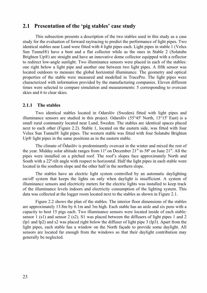
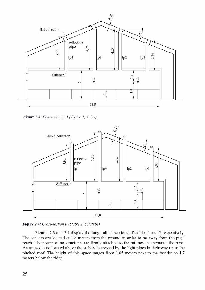
Figures 2.3 and 2.4 display the longitudinal sections of stables 1 and 2 respectively. The sensors are located at 1.8 meters from the ground in order to be away from the pigs’ reach. Their supporting structures are firmly attached to the railings that separate the pens. An unused attic located above the stables is crossed by the light pipes in their way up to the pitched roof. The height of this space ranges from 1.65 meters next to the facades to 4.7 meters below the ridge.

Figure 2.3: Cross-section A ( Stable 1, Velux).

Figure 2.4: Cross-section B (Stable 2, Solatube).

26

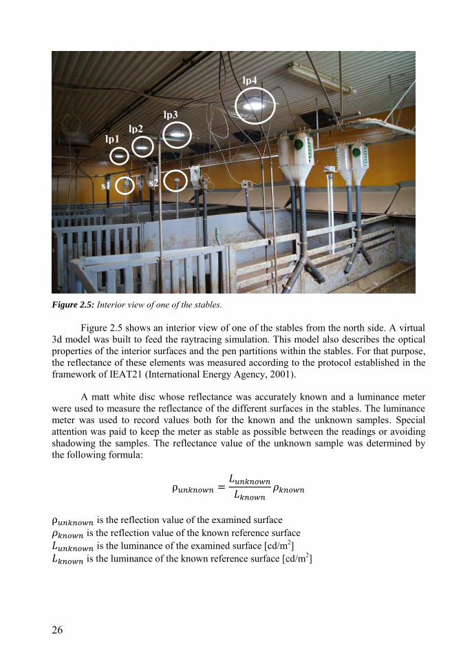
Figure 2.5 shows an interior view of one of the stables from the north side. A virtual 3d model was built to feed the raytracing simulation. This model also describes the optical properties of the interior surfaces and the pen partitions within the stables. For that purpose, the reflectance of these elements was measured according to the protocol established in the framework of IEAT21 (International Energy Agency, 2001).

A matt white disc whose reflectance was accurately known and a luminance meter were used to measure the reflectance of the different surfaces in the stables. The luminance meter was used to record values both for the known and the unknown samples. Special attention was paid to keep the meter as stable as possible between the readings or avoiding shadowing the samples. The reflectance value of the unknown sample was determined by the following formula:

is the reflection value of the examined surface is the reflection value of the known reference surface is the luminance of the examined surface [cd/m2] is the luminance of the known reference surface [cd/m2]

Figure 2.5: Interior view of one of the stables.

s1 s2

lp1 lp2

lp3

lp4

27

The results of the reflectance measurements are summarized in Table 2.1.

Table 2.1: Measured light reflectance of surfaces in the stable.

Partitions between pens (lower part) 22% Partitions between pens (upper part) 30% Pen floor (no straw) 14% Pen floor (some straw) 30% Pen floor (a lot of straw) 24% Pen floor (new straw) 32% Concrete floor 12% Slatted concrete floor 9% Concrete floor outside pen 19% Yellow walls 40% Ceiling (white corrugated steel plates) 65%

2.1.2 The light pipes This section addresses general aspects about light pipes and describes the specific

characteristics of the models used in these pig stables: Velux Sun Tunnel® and Solatube Brighten Up®.

Light pipes or TDGS consist of three main components: the collector, the reflective pipe caleed MLP and the diffuser (Figure 2.6). Table 2.2 displays the optical properties of both light pipe models used in this study. The function and main features of each of these components is further described below.

Figure 2.6: Diagrammatic representations of a Solatube light pipe (left) and scheme of a simple light pipe with its main components defined (right). Source: Solatube website.

28

Table 2.2: Optical properties of the assessed light pipe models.

Velux Sun Tunnel® (Rigid bend, Ø35cm)

Solatube Brighten Up® 290 DS (Ø35cm)

Source

Collector type Flat Dome Data provided by the manufacturing companies: Solatube® and Velux®

Collector light transmittance

87% 92%

Pipe light reflectance 98% (6% diffuse) 99% (fully specular) Diffuser light transmittance

81% 92%

Deflector light reflectance - 99% (fully specular)

Collectors:

The collector is a transparent element located at the external aperture of the pipe. Its main functions are daylight collection and protection of the light pipe from the impact of weather and dirt. It is usually made of a highly transmitting material, which can be flat or dome-shaped. In this case the light pipes in stable 1 (Velux) are provided with a flat collector while the ones in stable 2 (Solatube) have a dome collector.

The flat collector of Velux consists of a simple clear glass pane fastened at the light pipe upper aperture.

Figure 2.7 shows the dome-shaped collector of Solatube, which is molded with a variable prism optic that redirects sunlight from low solar altitudes into the pipe. This feature is proven to enhance the light efficiency of the light pipe for such conditions of low sun (Zhang, Muneer, & Kubie, 2002) (Lo Verso, Pellegrino, & Serra, 2011). This is an beneficial feature in the Scandinavian context. However, the predominance of overcast skies in winter, when the sun is lowest, substantially limits the advantages of using this system. Besides optimizing the collection of low sunlight these types of dome usually limit high angle sunlight to avoid visual discomfort from sunlight patches. In this case such high solar angles are inexistent, which might make this feature rather disadvantageous, as it is blocking part of the diffuse light from the sky.

Figure 2.7: Solatube dome collector fitted with reflector. Source: Solatube website.

29

The Solatube dome collector is equipped with a light deflector, which can be classified as an optical redirecting system (ORS). It is a laser-cut panel located within the dome collector and oriented towards the equator. Its purpose is to redirect low angle incident beam light into the pipe. Light penetration for low solar altitude angles (below 60º) is thus enhanced further (Lo Verso, Pellegrino, & Serra, 2011) (Edmonds, Moore, Smith, & Swift, 1995). This is advantageous for Southern Sweden where midday solar altitude in varies between 11º and 58º. However, the light deflector partly blocks the penetration of the diffuse light from the North. This is a critical point for the Scandinavian context where diffuse radiation accounts for about 50% the total annual radiation (Khellsson, 2002). It should be noted that the northernmost light pipe of stable 2 (lp4) was not fitted with a light deflector as direct sunlight is blocked from it by the pitched roof most of the year.

Both the collector dome and the reflector are ORS. Goniophotometric measurements are usually needed to define the light redirecting properties of ORS. In this case that information was not provided by the manufacturer. Given the lack of BTDF data their light deflective properties were not considered in the computer simulation. This simplification has a significant impact in the simulation results, which is discussed in a later chapter.

Mirrored Light Pipe (MLP):

The MLP is the pipe that transports daylight from the collector to the diffuser. Its design and optical properties are optimized to minimize the light losses. In this case, both assessed light pipe models have circular cross-sections, since this is the most common shape on the market. However, some studies recommend flattened cross-section pipes, which enhance the system performance at low solar altitudes (Swift, 2010).

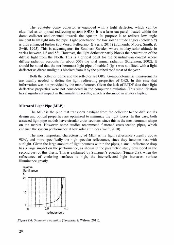
The most important characteristic of MLP is its light reflectance (usually above 98%), and more specifically the high specular reflectance, since they function best with sunlight. Given the large amount of light bounces within the pipes, a small reflectance drop has a large impact on the performance, as shown in the parametric study developed in the second part of this thesis. This is explained by Sumpner’s equation (Figure 2.8): when the reflectance of enclosing surfaces is high, the interreflected light increases surface illuminance greatly.

Figure 2.8: Sumpner’s equation (Tregenza & Wilson, 2011).

30

Another important characteristic for the performance of a light pipe is its aspect ratio, i.e. the diameter to length ratio. It determines the amount of light bounces in the light pipe. The recommended aspect ratio is < 1/10 and, according to some authors, it should never exceed 1/20 in order no reach a minimum light output (Mohelnikova, 2009). The conclusions of the parametric study are that this limit should be 1/15 in the Scandinavian context, due to the predominance of low solar altitudes. The aspect ratio of the light pipes installed in the pig stables ranged from 1/9 to 1/15. Cross-sections should never be less that 200 mm in diameter to avoid excessive light losses along the light guide. In this case, both models have a diameter of 350 mm.

Diffusers:

The light pipe diffuser is installed on the ceiling of the room to be illuminated and usually takes the form of an opal dome or a white, flat polycarbonate. Along with solar altitude, the diffuser choice determines the light output distribution of light pipes (Mohelnikova, 2009).

The exiting light distribution is affected by the shape and texture or pattern on the diffuser. Flat diffusers produce a narrower light beam while convex shapes allow for wider angles of light diffusion (Zhang, Muneer, & Kubie, 2002). On the other hand, the total light output from a flat diffuser is approximately 10-12% better than for a curved one (Robertson, Hedges, & Rideout, 2010). Fresnel diffusers or two component diffusers are intermediate solutions. They are especially beneficial for clear sky conditions only with modest disadvantages for diffuse incident light. They are equipped with a diffuse central part and clear rim area around it (Kocifaj, 2009). Lighting vertical surfaces can increase the perception of brightness in a space. Anisotropic diffusers can produce that effect (Akashi, Tanabe, Akashi, & Mukai, 2000) by spreading out the light beam.

The diffusers of the light pipes in the pig stables are flat and prismatic. Solatube’s diffuser produces a wider beam compared to Velux. This is suspected to be due to the OCS included in the Solatube collector, which is explained in further chapters.

Diffusers are also a type of OCS. As in the case of the dome collector, it is important to have the goniophotometric properties in order to accurately simulate the way light is scattered in space. Unfortunately this type of data is not always provided by the manufacturers. In this case it was only available for the diffuser of the Velux devices. The scattering properties of the Solatube diffusers were selected by choosing a default scheme from the simulation program (TracePro®) material library that roughly matched the light scattering pattern measured onsite.

31

Figure 2.8: Interior view of a light pipe diffuser.

32

2.2 Field measurements

This subsection describes how the illuminance and electricity consumption logging systems installed in the pig stables work. Three variables were logged constantly from December 2013 to March 2014 in the stables:

- Exterior illuminance (GHI): using a sensor located at an unobstructed area near the stable.

- Interior illuminance: using two sensors in each stable. Normally interior illuminance is measured horizontally at desk height (about 0.8 meters from the floor). In this case the sensors had to be placed higher (1.8 meters from the ground), i.e. away from the pigs reach.

- Electricity consumption of electric light system in each of the stables to assess the savings achieved by the installed light pipes.

The data logging system was connected to five illuminance meters (two in each stable and one outdoors) and two electricity meters (Figure 2.9). The data-logger acquires signal from the different sensors every 10 seconds. These values are stored in a cache memory (temporary memory). This type of data storage deletes the data used to calculate periodic averages once this average was calculated. Then this data is averaged every six minutes and each hour. These averaged values are saved in a non-volatile (permanent) storage.

Figure 2.9: Schematic representation of the data logging system.

33

The indoor illuminance at three points of each stable is retrieved using Hagner sensors TWP01T/SD2 (Figure 2.10). These are standard, cosine corrected illuminance sensors calibrated according to human eye sensitivity. Each sensor has an absolute sensitivity of about 120 pA/lux. The sensor is mounted in a water proof, (IP65) heated casing to avoid condensation and frost due to the low temperature in the stable. The casing also includes a built-in 8.5 W heater which prevents the formation of condensation on the surface. The sensors were bought for this project and calibrated in a certified laboratory with a stated accuracy ±3%. The current signal from each sensor goes to a signal amplifier (Hagner MCA-1600) which stabilizes and converts the amperage to a 0-2 VDC voltage. Each of the amplifier ports is specifically calibrated for a single sensor, so that the 0-2 VDC is proportionally adjusted to the range 0-2000 lux (e.g., 100 mV corresponds to 100 lux)

The horizontal global illuminance (GHI) is measured outdoors by a Hagner ELV-841 sensor. It consists of a Vλ-filtered and cosine corrected sensor and an amplifier with regulated current output (4-20 mA). It includes a waterproof case (IP65) and a heater to prevent condensation and to melt snow and ice in extreme meteorological conditions, supplied with 24V AC. The current output, which is already amplified, is then converted to a voltage through a 800 Ω external resistance. The Hagner ELV-841 was also bought for this project and calibrated in a certified laboratory. The range 4-20 mA corresponds to 0 – 200000 lux (non-linear) with an accuracy of ±3%.

Each stable was equipped with an individual electricity meter connected to the electric lighting system. The electrical light consumption was thus accounted for separately in the data logger. The output from the electricity meters was provided by both an LCD display plus a digital output which provided 1000 pulses/kWh. The digital output was connected to the digital ports of the central data logger, so that the electricity use was recorded in correlation to the illuminance. Each electricity meter was integrated with a daylight on/off switch. The daylight on/off switch used was a commercial product allowing the adjustment of an illuminance threshold below which the electric lighting is switched on. This threshold can be set at a value from 10-500 lux. The time delay for the switching was

Figure 2.11: Indoor illuminance sensor in one of the stables

34

also adjustable and it was set to a minute for this study. Both the illuminance threshold and time delay were analogically adjusted through a potentiometer.

The data logger is a Campbell Scientific CR1000. The logger receives voltage input from the lux meters while getting a pulse from the electricity meters. None of the output voltage ports are used to supply the sensors’ heaters, which are, instead, connected to specific transformer connected to the electricity network. The data logger is provided with the interface software LoggerNet 3.1.4., which allows the communication between the computer and data logger through a serial port. The voltages are read by the differential ports. The reading range is set to ±2500 mV with 250 µs of integration time. The resolution is 333 µV, with an accuracy of about ±1,5 mV.

35

2.3 Selection of raytracing method

This subsection describes general features of raytracing and its two versions: backward and forward raytracing. Then it states the limitations of backward raytracing to be applied to light pipes and some possible workarounds considered at the beginning of this study. Finally, the choice of forward raytracing is justified.

Raytracing consists in the simulation of light rays that are randomly sent in space to predict light levels or create realistic images. The physical context needs to be defined by a model specifying the geometry as well as the optical properties of surfaces: i.e. absorption, reflection, refraction, scatter and diffraction (Kolås, 2013). Light sources in this model also need to be defined and characterized.

The principles behind raytracing were stated by Albrecht Dürer in the 16th century applied to perspective on paintings. The first raytracing software dates back to the 1960s. It was developed by the Ballistic Research Laboratory (later the U.S. Army Research Laboratory). It was developed to assist the enormous bookkeeping required for shotline calculations. This early software was actually the computerization of an earlier research that set the foundation of raytracing developed in the 1950s by hand by Davidson C. Hardison. In 1979 Turner Whitted developed the first raytracing system to simulate global illumination. This system already included the possibility to generate reflections, refractions and shadows. In the last decades of the 20th century the development of raytracing techniques was increasingly applied to computer animations and to the film industry as a way to create photorealistic images. It is also widely used by the building design industry to generate photorealistic images (renderings) of prospective buildings or to predict lighting conditions from daylight and/or electric lights.

The interest of raytracing as a tool to evaluate complex optical systems has increased notably lately (Lo Verso, Pellegrino, & Serra, 2011) (Kolås, 2013). The increasing power of commercial computers has made it possible to spread the access to these new tools and significantly reduce simulation times. Many experts defend the suitability and accuracy of raytracing software to simulate complex daylighting systems like light pipes (Dutton & Shao, 2007) (Kohler, 2010) (Farrel, Norton, & Kennedy, 2004). This method can handle simultaneously many more variables than other methods: different locations and sky conditions, diffuser and collector geometry, complex optical properties, bends in the pipe, etc.

The application of raytracing requires a detailed characterization of the optical properties of all relevant elements, which cannot always be done in the case of light pipes due to lack of information from manufacturers. Light pipes are frequently fitted with ORS to redirect the light into the pipe (collector) or spread it out into a space (diffuser). All of this requires a meticulous characterization of these elements though goniophotometric measurements and resulting BSDF data. Raytracing simulation programs can use the output of these measurements to simulate the light pipes performance (De Boer, 2003).

However, goniophotometric measurements are expensive and require specialized instruments and laboratories. However, it is important that this data is provided by the manufacturer (Lo Verso, Pellegrino, & Serra, 2011) as it will make it possible for prospective buyers to estimate the system’s performance.

36

Raytracing can be applied in two different ways: backward and/or forward. Backward raytracing is much more common. It is called ‘backward’ because the rays are emitted from the end point or point of view instead of the light source. The scattered rays thus go through a limited number of bounces (usually 3 to 5) throughout the model (Kolås, 2013), which greatly reduces the number of rays needed since all light rays falling outside the main view are not simulated. If they hit a light source, the light contribution of that source is added up in the point of view. The accuracy of the results depends on the amount of rays traced. Backward raytracing is usually preferred because in most applications it requires fewer rays to reach the same accuracy as forward raytracing.

However, many authors advice against the use of backward raytracing to analyze complex daylighting systems like light pipes, where many light bounces are expected (Kolås, 2013) (Mardaljevic, Heschong, & Lee, 2009). In order to be able to simulate light pipes, the number of light bounces needs to be increased significantly, with consequent lengthening of simulation times. Moreover, in backward raytracing, the chance of a ray hitting the sun in these conditions is very low. Direct sunlight is therefore not properly simulated with this technique.

At the beginning of this study, two different approaches were considered to work around the problem of accounting for direct sunlight in these complex systems using backward raytracing. Both approaches were dismissed for different reasons and finally forward raytracing was selected as the most suitable option. The two options considered were the following:

- 1. Using a discrete sky patch subdivision, such as the Tregenza scheme (Figure 2.12), with the sun contribution distributed over the nearest patches. This way the direct sunlight is more effectively represented, and ‘finding the sun’ less of a problem. A disadvantage of this method is that it implies a more smoothed out distribution of the contribution of the direct sun. However, in this case this should not be crucial. Nonetheless, this system still requires a large amount of bounces to go through the pipe, with the subsequent increase in simulation times, which is why it was dismissed as a suitable method in the present study.

Figure 2.12: Example of a Tregenza patch subdivision of a sky dome.

37

- 2. Calculating the BTDF function of each light pipe and replacing it in the model by a diffuser with these bi-directional optical properties. This method avoids the need to increase the ambient bounces and permits a more accurate representation of direct sunlight. Nonetheless, this method was discarded for being too complex and requiring a very advanced knowledge of computer daylight simulation, which limits its actual applicability.

Finally, forward raytracing was selected as the most suitable method to simulate light output from light pipes on account of its relative simplicity, good accuracy – also of the direct sun contribution – and its capacity to simulate large amounts of light bounces keeping reasonable simulation times.

Forward raytracing sends rays from light sources and through multiple bounces in the virtual model to determine luminance of illuminance (Figure 2.12). At each interaction with the model, rays can be subject to absorption, reflection, refraction, diffraction and scatter. As the rays spread through the model, the program keeps track of the optical flux associated with each ray (Lambda Research Corporation, 2014). It uses virtual surfaces called pupils to reduce the total number of rays going from the light source (the sun or the sky) to the model.

The program used in this case was TracePro® Expert 7.4.1 Release (TracePro®), which is the most advanced forward raytracer at the moment. Originally the software was designed to simulate electric light and presented some limitations to simulate daylight, since sky-light distributions had to be defined manually (Kolås, 2013). However, this hindrance was overcome in latest version, which is equipped with a new capability called solar emulator. This new capability permits to simulate direct sunlight as well as diffuse light from a variety of sky types.

One of the main advantages of the solar emulator is that it can simulate large amounts of light bounces keeping reasonably short simulation times. This is achieved by simulating only the rays directed towards the openings of the virtual model of the building. The targets placed over the openings where rays are directed to are called pupils or ports. The remaining rays that would never enter the building are thus not simulated.

Forward raytracing does not create the problem of ‘not finding the sun’, which was one of the main drawbacks of backward raytracing. In theory, the sun contribution is correctly simulated as rays are directly casted from the sun. In this case, the results show a certain overestimation of sun contribution for high solar altitudes, which might be caused by the system used to size the sun contribution. A future work will be undertaken to solve this issue.

38

2.4 Description of the simulation method utilized

This subsection describes the way forward raytracing was applied in this particular case using TracePro® following three steps:

- A. Building the virtual model - B. Defining the light sources - C. Defining the pupils (targets where light rays from sun and sky are aimed at) and

sensors (areas where the illuminance is assessed)

A. Building the virtual model:

The virtual model needs to include the most relevant elements in the model. Figure 2.14 shows an axonometric view of the virtual model of stable 2. The room envelope, the pens partitions, and the pens covers were modeled. Figure 2.13 shows an interior view of one of the stables. Some elements that can be seen in the picture, like feeding systems for the pigs and several other pipes hanging from the ceiling, were not considered in the virtual model. This might entail some error in the simulation results. However, this error might not be substantial given the size and position of the omitted elements with respect to the sensors. The 3d models of the stables were modelled using Rhinoceros® and then exported to TracePro® through an ACIS (*.sat) file. Light pipes were modeled as accurately as possible including the collectors, MLP and diffusers.

Figure 2.13: Interior view of one of the stables fitted with light pipes.

Feeding system

Pen covers

Sensor 1

39

The optical properties of the modelled elements also need to be specified in the program to account for the light interactions with these elements. The elements of the light pipes require accurate optical characterization as they are determinant for the amount of daylight reaching the room and the way this light is distributed.

In the case of complex optical systems like ORS a goniophotometric specification is also required though a BSDF file. BSDF information for the ORS included in the light pipes was only available in the case of the Velux diffuser. The BSDF data provided by the manufacturer was introduced in the program using the BSDF Converter utility of TracePro®. The rest of the transparent elements in the light pipes were defined using the fraction of absorbed/transmitted light (Table 2.3). This information was provided by the manufacturers. In the case of the Velux flat collector this information was sufficient to characterize it. In the case of the dome collectors and diffusers of the Solatube light pipes, this information does not suffice to accurately reproduce their interaction with light. As previously stated, a BSDF file would be needed for that purpose. Instead, a standard diffuser surface property from the program library was applied to the Solatube diffuser. No BSDF properties were applied to the collector dome for the same reason. This limitation in available information had a significant effect on the results, which is discussed further down in this document.

Table 2.3: Optical characterization of the translucent and transparent materials in TracePro®.

Material Elements Thickness (mm)

Light transmittance

Absorption Coef. (per mm)

Acrylic plastic Solatube diffuser and collector

3 92% 0.001

SGG Bioclean Velux collector and diffuser (lower pane)

4 87% 0.04

PET GAG plastic

Velux diffuser (upper pane) 1 92% 0.001

Figure 2.14: TracePro® model of one of the stables.

40

The reflectance of the elements included in the model was specified. All the elements in the stables were treated as Lambertian reflectors. This means that the reflectance data previously measured was introduced as being 100% diffuse. This is a common simplification that normally does not introduce significant errors. The MLPs, however, require a more detailed characterization, specifying separately diffuse and specular reflectance. The absence of this specific data was found to cause large discrepancies between simulation and measurements.

B. Defining the light sources:

The solar emulator utility of TracePro® is used to simulate daylight from both the sky dome and the sun. Latitude, longitude, date, time, time zone, north vector and zenith vector need to be specified to locate the sun position and sky luminance distribution in reference to the model.

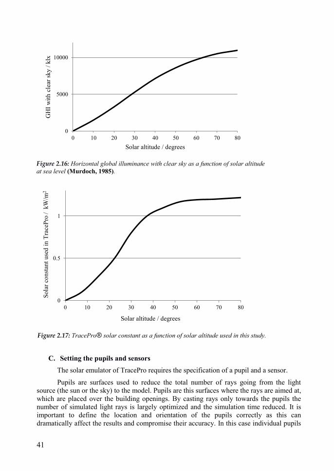
The sky luminance distribution is defined by selecting from a catalogue of predefined sky models (Figure 2.15). In this case, the overcast and clear skies of the Igawa all-sky models are used. In addition, a range of 50,000-80,000 rays were used in the different simulations as a sufficient number of rays to reach accurate results.

The solar model is defined by a solar constant expressed in W/m2. The default value (1,067 W/m2) needs to be adapted for each specific location according to elevation and solar altitude. Figure 2.16 displays the GHI at sea level according to the solar elevation angle. Lund has low elevation of about 60m above sea level and can therefore be assimilated to a place at sea level. The solar constant values introduced in TracePro® for a place located at sea level were estimated as follows. GHIs for different solar altitudes on a clear day were simulated in the program. The solar constant was then adjusted for each solar altitude to reach the targeted GHIs shown in Figure 2.16. The resulting values for the solar constant introduced in TracePro® are plotted in Figure 2.17. This method to calculate the solar constant will be reexamined in the future as it is suspected to have caused some overestimation of direct sunlight for high solar altitudes.

A range of 10,000-30,000 rays was used in the simulations in order to reach a sufficient level of accuracy.

Figure 2.15: Example of clear (right) and overcast (left) Iwaga all-sky model luminance distribution.

41

C. Setting the pupils and sensors

The solar emulator of TracePro requires the specification of a pupil and a sensor.

Pupils are surfaces used to reduce the total number of rays going from the light source (the sun or the sky) to the model. Pupils are this surfaces where the rays are aimed at, which are placed over the building openings. By casting rays only towards the pupils the number of simulated light rays is largely optimized and the simulation time reduced. It is important to define the location and orientation of the pupils correctly as this can dramatically affect the results and compromise their accuracy. In this case individual pupils

0

5000

10000

0 10 20 30 40 50 60 70 80

GH

I with

cle

ar sk

y / k

lx

Solar altitude / degrees

0

0.5

1

0 10 20 30 40 50 60 70 80

Sola

r con

stan

t use

d in

Tra

cePr

o /

kW/m

2

Solar altitude / degrees

Figure 2.16: Horizontal global illuminance with clear sky as a function of solar altitude at sea level (Murdoch, 1985).

Figure 2.17: TracePro® solar constant as a function of solar altitude used in this study.

42

are placed over the exterior apertures of each of the four pipes in each stable. This way the light contribution of each of them on the sensors was considered separately.

The sensors were modelled as 300x300mm horizontal squares located in the virtual model in the same position as the actual sensors. Forward raytracing estimates the illuminance on a surface by adding up the contribution of all light rays meeting that surface Figure 2.18 shows rays traced (red dots) on one of the sensors (dotted square). This image was obtained from one of the simulations launched with TracePro. This size was considered large enough to be hit by a sufficient amount of light rays so their value can be averaged to a reasonably accurate value. The actual sensors only ‘sees’ the light coming from their upper hemisphere, light coming below is not captured. For this reason only the rays hitting the top side of the square were considered here.

Figure 2.18: Example of simulation result of TracePro® for one of the sensors.

43

2.5 Sources of error

This subsection discusses the error sources encountered during the course of this research project and how the sensor readings and the simulation results were handled to minimize these errors. In most cases the simulation results and the measurements showed discrepancies between 10% and 20%. It should be pointed out that the accumulation of error sources encountered might create uncertainties close to those values. The acknowledgement of the number and magnitude of errors is required to judge the accuracy of the comparison. A list of acknowledged error sources follows:

- A. Variability of measurements

- B. Dirtiness deposition on the indoor sensors

- C. Daylight on/off sensor

- D. ‘Inaccuracies’ in the virtual model

- E. Optical characterization of the light pipes

- F. Location of the ports

- G. Use of generic sky models

A. Variability of measurements

A total number of eleven different times were picked to compare measurements and simulation results. The readings of the sensors, averaged every 6 minutes, show high levels of variability over time, especially with overcast skies. To try to minimize these fluctuations three consecutive measurements were averaged in each of the times picked to be compared to the simulation results.

Table 2.4 displays the eleven times selected, of which five correspond overcast skies (OC) and six to clear skies (CL). The measurement data available during this research project corresponds to the period between the end of December 2013 and mid-March 2014. Two criteria were used to select the eleven selected times. The first one is that they should be as close as possible to either pure overcast or clear skies. It should be noted that TracePro only simulates generic sky types. This means that their sky clearness indexes (Kt) of the selected times (Kt) should be close to 0 (purely clear) or 1 (purely overcast). The sky clearness data were provided by the Swedish Meteorological and Hydrological Institute (SMHI). The second criterion was that they correspond to different times during the day and different solar altitudes in the case of clear skies. This variety of sun positions was considered important for the evaluation.

Significant fluctuations between consecutive measurements were noticed in most cases. That is why it was considered appropriate to average three consecutive measurements (five in OC1) to reduce the uncertainty caused by the fluctuations observed in the readings. For instance, for the moment OC2 (February 19th at 16:12), the values considered were 16:06, 16:12 and 16:18.

44

Table 2.4: List of times considered (OC stands for overcast and CL for clear sky). Name Kt Date Time Solar altitude OC1 0.92 11-Feb-2014 14:12 - OC2 1 19-Feb-2014 16:12 - OC3 1 03-Feb-2014 15:00 - OC4 1 21-Jan-2014 10:00 - OC5 1 01-Jan-2014 12:00 - CL1 0.14 04-Feb-2014 12:00 17.45˚ CL2 0 10-Feb-2014 15:30 9.06˚ CL3 0.01 10-Feb-2014 13:00 18.90˚ CL4 0.03 25-Feb-2014 14:12 21.30˚ CL5 0.03 25-Feb-2014 17:00 2.92˚ CL6 0.01 12-Mar-2014 10:48 28.16˚

B. Dirtiness deposition on the indoor sensors

Sensor dirt factors (SDF) were calculated to account for dirt accumulation on the sensors located in the pig stables. Pigs cause a significant dirt accumulation on the sensors dome. After cleaning the sensors, the dirt continues to accumulate on the sensors until a staff member cleans them again. These fluctuations of dirt levels are considerable. This is why it was important to assess the dirt levels individually at each of the four indoor sensors for each of the days of the eleven times compared.

The dirt sensor factors were calculated taking as reference the moment OC1 (February 11th), when the sensors had just been thoroughly cleaned. This is why this moment is the only one that does not use a SDF. For the other ten measurement times, the SDF was calculated taking as reference the reading corresponding to February 12th at 09:18 AM, which is shortly after the OC1. This specific moment was picked as reference because it has light conditions that happen each day: the electric lights were on and the daylight levels outdoor were low, (GHI = 8,081 lux). The GHI is measured by a fifth sensor located near the stables at an unobstructed area. A similar situation (lights on and about 8,000 GHI) was picked for each of the days considered. Then, the SDF was calculated according to the following formula:

is the dirt sensor factor on a chosen day

is the illuminance reading from the sensor at the reference moment (February 12th at 09:18; lights were on and the GHI was 8,018 lux)

is the illuminance reading from the sensor on the chosen day at a moment when the electric lights were on and the GHI was approximately 8,000 lux.

45

Table 2.5 displays the SDF calculated for each of the eleven times considered and each of the four indoor sensors.

Table 2.5: Sensor Dirt factors (SDF) of the illuminance sensors for each considered time.

Moment Date Sensor 1a Sensor 1b Sensor 2a Sensor 2b E(lx) SDF E(lx) SDF E(lx) SDF E(lx) SDF

OC1* 11-Feb 620.5 - 346.5 - 340.0 - 97.3 - OC2 19-Feb 514.8 1.21 301.5 1.15 277.4 1.23 85.9 1.13 OC3 03-Feb 439.9 1.41 224.2 1.55 232.6 1.46 70.2 1.39 OC4 21-Jan 490.2 1.27 306.9 1.13 280.4 1.21 96.8 1.01 OC5 01-Jan 526.2 1.20 293.1 1.18 272.9 1.25 93.7 1.04 CL1 04-Feb 433.6 1.43 224.2 1.55 232.6 1.46 70.2 1.39 CL2,3 10-Feb 442.4 1.40 270.2 1.28 247.7 1.37 76.1 1.28 CL4,5 25-Feb 432.2 1.44 230.0 1.51 200.2 1.70 92.1 1.06 CL6 12-Mar 440.3 1.41 210.1 1.65 218.0 1.56 60.2 1.62 (*) reference value (clean sensors)

C. Daylight on/off sensor

The daylight on/off sensor consists of a commercial photodiode connected directly to the electric light switch. It presents two main issues in this particular installation: In the first place, the threshold value is much lower than the light levels provided by the lighting systems, which creates a problem of instability in the system. This was solved by placing the daylight on/off sensors in the attic instead of in the stables. The switch threshold was set at a low value for indoor environment (40 lux), which was considered sufficient for pigs. On the other hand, the electric lighting provides a much higher value of around 600 lux at pig height.

If the photodiodes were placed in the stable, they would be affected inevitably by the electric lights by producing a senseless loop of on/off states of the electric lights (Figure 2.19-2.21). The low illuminance levels reaching the sensors would activate the lights, and this activation would in turn produce a high light level in the sensor that would lead to the lights being turned off shortly afterwards, starting the loop again. This anomaly would not happen in normal applications, e.g. offices with threshold matching the light levels given by the electric light system (about 500 lux). In this particular case this problem is solved by placing the photodiodes of both stables in the attic right above the stables (Figure 2.22). This space relies exclusively on daylight and is not affected by the stable electric lights (Figure 2.23). The sensor threshold was set by calculating the illuminance ratio between the photodiode position and a representative point in the stable.

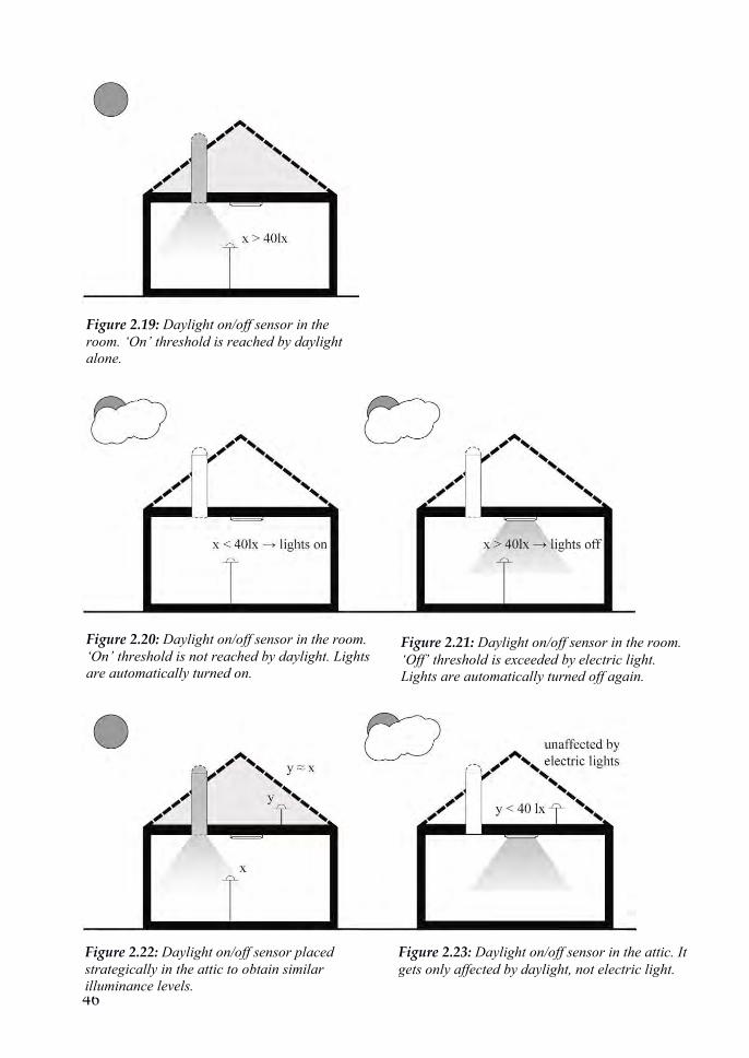
46

Figure 2.19: Daylight on/off sensor in the room. ‘On’ threshold is reached by daylight alone.

Figure 2.20: Daylight on/off sensor in the room. ‘On’ threshold is not reached by daylight. Lights are automatically turned on.

Figure 2.21: Daylight on/off sensor in the room. ‘Off’ threshold is exceeded by electric light. Lights are automatically turned off again.

Figure 2.23: Daylight on/off sensor in the attic. It gets only affected by daylight, not electric light.

Figure 2.22: Daylight on/off sensor placed strategically in the attic to obtain similar illuminance levels.

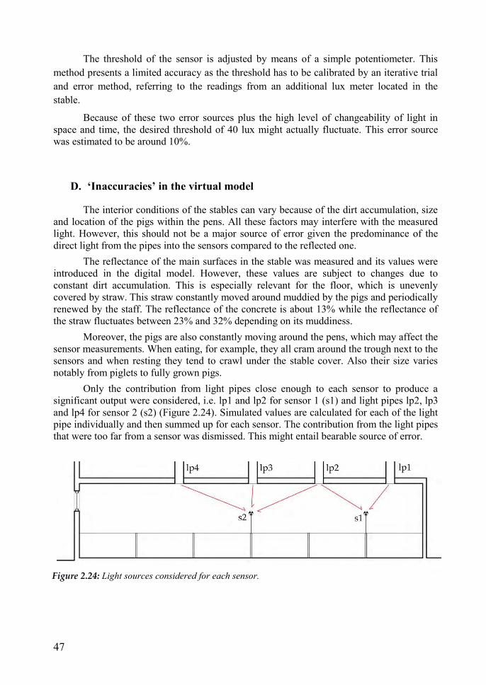
47

The threshold of the sensor is adjusted by means of a simple potentiometer. This method presents a limited accuracy as the threshold has to be calibrated by an iterative trial and error method, referring to the readings from an additional lux meter located in the stable.

Because of these two error sources plus the high level of changeability of light in space and time, the desired threshold of 40 lux might actually fluctuate. This error source was estimated to be around 10%.

D. ‘Inaccuracies’ in the virtual model The interior conditions of the stables can vary because of the dirt accumulation, size and location of the pigs within the pens. All these factors may interfere with the measured light. However, this should not be a major source of error given the predominance of the direct light from the pipes into the sensors compared to the reflected one. The reflectance of the main surfaces in the stable was measured and its values were introduced in the digital model. However, these values are subject to changes due to constant dirt accumulation. This is especially relevant for the floor, which is unevenly covered by straw. This straw constantly moved around muddied by the pigs and periodically renewed by the staff. The reflectance of the concrete is about 13% while the reflectance of the straw fluctuates between 23% and 32% depending on its muddiness. Moreover, the pigs are also constantly moving around the pens, which may affect the sensor measurements. When eating, for example, they all cram around the trough next to the sensors and when resting they tend to crawl under the stable cover. Also their size varies notably from piglets to fully grown pigs.

Only the contribution from light pipes close enough to each sensor to produce a significant output were considered, i.e. lp1 and lp2 for sensor 1 (s1) and light pipes lp2, lp3 and lp4 for sensor 2 (s2) (Figure 2.24). Simulated values are calculated for each of the light pipe individually and then summed up for each sensor. The contribution from the light pipes that were too far from a sensor was dismissed. This might entail bearable source of error.

Figure 2.24: Light sources considered for each sensor.

48

E. Source of error due to the optical characterization of the light pipes

An accurate characterization of geometry and optical properties of all the light pipes’ components is essential to reach simulation results reasonably close to the measurements. Goniophotometric properties of the diffusers and collectors (if provided with light bending properties) are needed to increase the reliability of the simulations. Unfortunately, this information is not always provided, as was the case for the components of the Solatube light pipes under investigation. This had a clear effect on the results that will be discussed later on in this thesis. Light pipe reflectance is normally provided by the manufacturers based on laboratory measurements performed in optimal conditions. However, the conditions of the product may not be as good in real projects due to a less careful construction and handling of the materials. Small variations in the reflectance of the interior coating largely affect the system total LLF because of the large amount of light bounces in the pipes. Note that a reduction factor of 5% was applied to take consideration of dirt accumulation in the light pipe.

F. Source of error due to the location of the ports The ports or pupils are the targets where rays are aimed at in forward raytracing

simulations. In the case of this study, the pupils were placed over the collectors of each of the light pipes. This worked well for the flat collector of Velux (Figure 2.25). However, due to the convex shape of its collector in the case of Solatube, it was a challenging task to accurately gather all rays from both sun and sky with a satisfying accuracy and reasonable simulation time. Placing a horizontal surface aligned with top aperture of the pipe resulted in having the sun rays missing the reflector (dashed lines in Figure 2.26).

Two different approaches were tried to solve this. Each of them produced unwanted effects like missing part of the sky rays or large increases in the simulation time. Finally, a combination of both approaches was used to minimize negative side effects.

The first approach consisted of tilting the pupil towards the South. This way, the rays hitting the reflector were traced by the program. However, the rays from the North of the sky dome on the sides of the reflector were missed (Figure 2.27). The second approach consisted of increasing the size of the pupil (Figure 2.28). However, this largely increased the simulation time required. As the diameter of the pupil was increased the amount of rays required to reach the same accuracy rised up rapidly because most of the rays never reached the light pipe and were thus wasted. Finally, a combination of both approaches was chosen to minimize the amount of missed and wasted rays, see Figure 2.29.

49

Figure 2.25: pupil (dotted line) over Velux flat collector.

Figure 2.26: pupil located at the base of the Solatube dome collector.

Figure 2.27: pupil turned to capture the sun rays reflected on the reflector.

Figure 2.28: pupil enlarged to capture the sun rays reflected on the reflector.

SELECTED OPTION for the flat collector

(Velux)

Discarded option for the dome collector

(Solatube): the rays that are supposed to

hit the reflector are not traced.

Discarded option for the dome collector

(Solatube): although the rays that hit the

reflector are traced, a large number of the

casted rays do not enter the light pipe.

Discarded option for the dome collector

(Solatube): although the rays that hit the

reflector are traced, a part of the rays

from the sky dome are missed.

50

G. Use of generic sky models

This project uses generic sky models of clear and overcast skies (Iwaga all-sky model) to simulate luminance from the sky dome. This entails an intrinsic error source, as the actual GHI and the luminance distribution is unique for each time and location. Intermediate skies were not simulated because of their high level of variability, which makes generic models very different from actual conditions.

The difference in GHI between the actual and simulated sky was adjusted using a correction factor according to the following formula:

The measured GHI was obtained from a 5th illuminance sensor located outdoors.

Even though a GHI correction factor was used, the accuracy of the generic sky models to simulate the actual sky conditions is not perfect. These models represent ideal luminance distributions that very seldom occur in reality. This adds a certain level of uncertainty to this validation process. For this reason, the times used in the comparisons of this study were selected according to how close they were to pure overcast or clear skies. This was done by picking the times with sky clearness indexes closer to 1 or 0 respectively. The sky clearness indexes (Kt) were provided by the Swedish Meteorological and Hydrological Institute (SMHI) for Lund.

An alternative to generic sky models are actual HDR images of the simulated skies (Inanici, 2010). This method allows an accurate representation of the exact luminance distribution of each specific sky. Figure 2.30 shows some examples of HDR images of real skies. This method was not used in this study but could be tested in future validation work.

Figure 2.29: pupil enlarged and turned to capture the sun rays on the collector minimizing wasted rays and missed rays from the sky dome.

SELECTED OPTION for the dome

collector (Solatube): the rays that hit the

reflector are traced, the amount of

wasted rays is much less than in Figure

2.26 and the amount of rays from the sky

dome missed are less that in Figure 2.27.

51

Figure 2.30: examples of conventional sky images (above) and their respective HDR images (below) (Inanici, 2010).

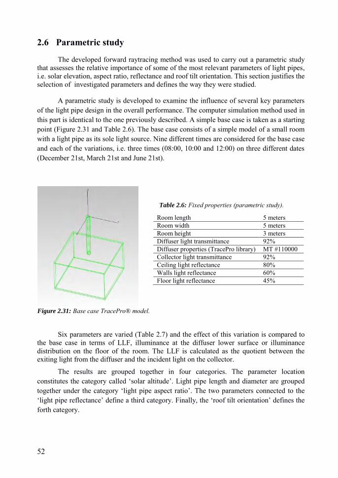
52

2.6 Parametric study

The developed forward raytracing method was used to carry out a parametric study that assesses the relative importance of some of the most relevant parameters of light pipes, i.e. solar elevation, aspect ratio, reflectance and roof tilt orientation. This section justifies the selection of investigated parameters and defines the way they were studied.

A parametric study is developed to examine the influence of several key parameters of the light pipe design in the overall performance. The computer simulation method used in this part is identical to the one previously described. A simple base case is taken as a starting point (Figure 2.31 and Table 2.6). The base case consists of a simple model of a small room with a light pipe as its sole light source. Nine different times are considered for the base case and each of the variations, i.e. three times (08:00, 10:00 and 12:00) on three different dates (December 21st, March 21st and June 21st).

Table 2.6: Fixed properties (parametric study).

Room length 5 meters Room width 5 meters Room height 3 meters Diffuser light transmittance 92% Diffuser properties (TracePro library) MT #110000 Collector light transmittance 92% Ceiling light reflectance 80% Walls light reflectance 60% Floor light reflectance 45%

Six parameters are varied (Table 2.7) and the effect of this variation is compared to the base case in terms of LLF, illuminance at the diffuser lower surface or illuminance distribution on the floor of the room. The LLF is calculated as the quotient between the exiting light from the diffuser and the incident light on the collector.

The results are grouped together in four categories. The parameter location constitutes the category called ‘solar altitude’. Light pipe length and diameter are grouped together under the category ‘light pipe aspect ratio’. The two parameters connected to the ‘light pipe reflectance’ define a third category. Finally, the ‘roof tilt orientation’ defines the forth category.

Figure 2.31: Base case TracePro® model.

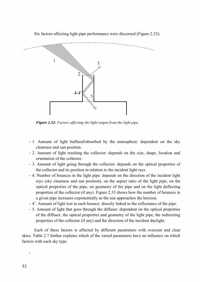
53

Six factors affecting light pipe performance were discerned (Figure 2.32):

- 1. Amount of light buffered/absorbed by the atmosphere: dependent on the sky clearness and sun position.

- 2. Amount of light reaching the collector: depends on the size, shape, location and orientation of the collector.

- 3. Amount of light going through the collector: depends on the optical properties of the collector and its position in relation to the incident light rays.

- 4. Number of bounces in the light pipe: depends on the direction of the incident light rays (sky clearness and sun position), on the aspect ratio of the light pipe, on the optical properties of the pipe, on geometry of the pipe and on the light deflecting properties of the collector (if any). Figure 2.33 shows how the number of bounces in a given pipe increases exponentially as the sun approaches the horizon.

- 4’. Amount of light lost in each bounce: directly linked to the reflectance of the pipe. - 5. Amount of light that goes through the diffuser: dependent on the optical properties

of the diffuser, the optical properties and geometry of the light pipe, the redirecting properties of the collector (if any) and the direction of the incident daylight.

Each of these factors is affected by different parameters with overcast and clear skies. Table 2.7 further explains which of the varied parameters have an influence on which factors with each sky type.

-

Figure 2.32: Factors affecting the light output from the light pipe.

54

Figure 2.33: Dependence of the number of reflections in a pipe (aspect ratio 1/11.25) on the zenith angle. Zenith angle = 90 – solar altitude (Kómar & Darula, 2012).

Parameter varied

Base case value Variations

Factors influenced (clear sky)

Factors influenced (overcast)

Category

Location (latitude)

Lund (56°N)

Helsinki (60°N) Frankfurt (50°N) Bordeaux (45°N) Barcelona (41°N) Malaga (37°N)

1, 2, 3, 4, 5 1

Solar altitude

Light pipe length

4.5m 3m 6m

2, 4 2, 4 Light pipe aspect ratio Light pipe

diameter 350mm 200mm

500mm 2,4 2,4

Total pipe reflectance

98% 99.7% 96.3%

4’ 4’ Light pipe reflectance Spec. refl. +

diff. refl. 92%+6% 98%+0%

86%+12% 4, 4’, 5 4, 4’, 5

Roof tilt orientation

Horizontal 30° South 30° East 30° West 30° North

2 2

Roof pitch

Table 2.7: Varied parameters, categories and affected factors.

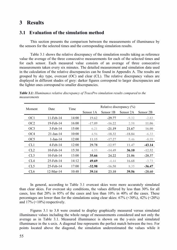
55

3 Results

3.1 Evaluation of the simulation method

This section presents the comparison between the measurements of illuminance by the sensors for the selected times and the corresponding simulation results.

Table 3.1 shows the relative discrepancy of the simulation results taking as reference value the average of the three consecutive measurements for each of the selected times and for each sensor. Each measured value consists of an average of three consecutive measurements taken every six minutes. The detailed measurement and simulation data used in the calculation of the relative discrepancies can be found in Appendix A. The results are grouped by sky type, overcast (OC) and clear (CL). The relative discrepancy values are displayed in different shades of grey: darker figures correspond to larger discrepancies and the lighter ones correspond to smaller discrepancies.

Table 3.1: Illuminance relative discrepancy of TracePro simulation results compared to the measurements

In general, according to Table 3.1 overcast skies were more accurately simulated than clear skies. For overcast sky conditions, the values differed by less than 30% for all cases, less that 20% in 85% of the cases and less than 10% in 40% of the cases. These percentages are lower than for the simulations using clear skies: 67% (<30%), 42% (<20%) and 17% (<10%) respectively.

Figures 3.1 to 3.8 were created to display graphically measured versus simulated illuminance values including the whole range of measurements considered and not only the average as in Table 3.1. Measured illuminance is shown on the y-axis and simulated illuminance in the x-axis. A diagonal line represents the perfect match between the two. For points located above the diagonal, the simulation underestimated the values while it

Moment Date Time Relative discrepancy (%) Sensor 1A Sensor 1B Sensor 2A Sensor 2B

OC1 11-Feb-14 14:00 19.62 -29.77 -9.32 -2.83 OC2 19-Feb-14 16:00 -17.09 -16.22 2.58 11.06 OC3 3-Feb-14 15:00 6.21 -21.19 21.67 16.00 OC4 21-Jan-14 10:00 4.56 -18.32 -18.84 -6.33 OC5 1-Jan-14 12:00 11.15 -17.27 5.46 -8.59 CL1 4-Feb-14 12:00 29.78 -12.97 11.47 -43.14 CL2 10-Feb-14 15:30 4.55 -14.49 36.10 -12.52 CL3 10-Feb-14 13:00 35.66 24.22 21.06 -20.37 CL4 25-Feb-14 14:12 49.69 -4.44 16.68 -3.73 CL5 25-Feb-14 17:00 -32.98 -16.50 8.35 -36.47 CL6 12-Mar-14 10:48 39.14 23.10 39.56 -28.60

56

overestimated the values for points located below the diagonal. Individual measurements are shown as black crosses. In contrast to the previous table, this way to display the results allows the comparison of the simulation with the whole range of measurements.

The range of measurement values is higher for overcast conditions compared to clear sky conditions. It is also higher for sensors located between two light pipes (1A and 2A) than for sensors located right below the light pipes (1B and 2B).

In spite of that high variability, the trend of the measurements seems to match that of the simulation results for overcast conditions on all sensors (Figures 3.1 to 3.4).

In the case of clear skies, the trend of the simulated illuminance seems to differ from that of the measured one for three of the four sensors. In sensors 1A and 2A (Figures 3.5 and 3.7 respectively), there is a trend to overestimate the values for higher illuminances. In the case of sensor 2B an inverse trend (progressive underestimation) is seen on Figure 3.8. The trend for the simulations in Sensor 1B (Figure 3.6) seems to approximately follow that of the measurements.

Figure 3.1: Comparison of measured and simulated illuminance in sensor 1A with overcast conditions. Simulation launched with TracePro.

0

50

0 50

Mea

sure

d ill

umin

ance

/ lx

Simulated illuminance / lx

Sensor 1A - overcast

57

Figure 3.2: Comparison of measured and simulated illuminance in sensor 1B with overcast conditions. Simulation launched with TracePro.

Figure 3.3: Comparison of measured and simulated illuminance in sensor 2A with overcast conditions. Simulation launched with TracePro.

0

50

100

0 50 100

Mea

sure

d ill

umin

ance

/ lx

Simulated illuminance / lx

Sensor 1B - overcast

0

50

0 50

Mea

sure

d ill

umin

ance

/ lx

Simulated illuminance / lx

Sensor 2A - overcast

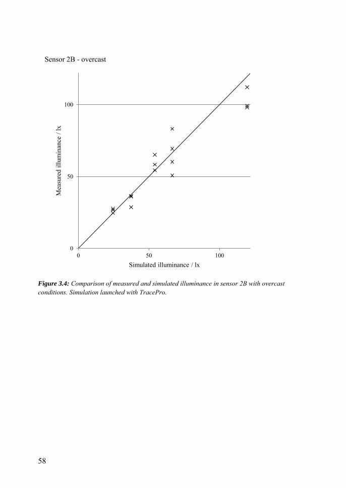
58

Figure 3.4: Comparison of measured and simulated illuminance in sensor 2B with overcast conditions. Simulation launched with TracePro.

0

50

100

0 50 100

Mea

sure

d ill

umin

ance

/ lx

Simulated illuminance / lx

Sensor 2B - overcast

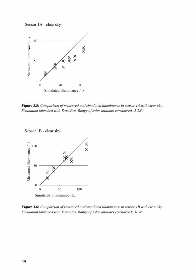
59

Figure 3.5: Comparison of measured and simulated illuminance in sensor 1A with clear sky. Simulation launched with TracePro. Range of solar altitudes considered: 3-28°.

Figure 3.6: Comparison of measured and simulated illuminance in sensor 1B with clear sky. Simulation launched with TracePro. Range of solar altitudes considered: 3-28°.

0

50

100

0 50 100

Mea

sure

d ill

umin

ance

/ lx

Simulated illuminance / lx

Sensor 1A - clear sky

0

50

100

0 50 100

Mea

sure

d ill

umin

ance

/ lx

Simulated illuminance / lx

Sensor 1B - clear sky

60

Figure 3.7: Comparison of measured and simulated illuminance in sensor 2A with clear sky. Simulation launched with TracePro. Range of solar altitudes considered: 3-28°.

0

50

100

150

200

0 50 100 150 200

Mea

sure

d ill

umin

ance

/ lx

Simulated illuminance / lx

Sensor 2A - clear sky

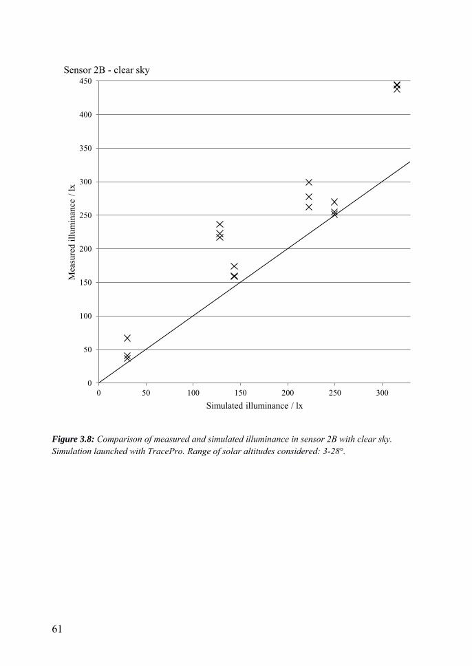
61

Figure 3.8: Comparison of measured and simulated illuminance in sensor 2B with clear sky. Simulation launched with TracePro. Range of solar altitudes considered: 3-28°.

0

50

100

150

200

250

300

350

400

450

0 50 100 150 200 250 300

Mea

sure

d ill

umin

ance

/ lx

Simulated illuminance / lx

Sensor 2B - clear sky

62

The average absolute deviation (AAD) for the measured values was calculated to estimate the variability of light levels at each of the sensors and sky types. This value was expressed as a percentage of the mean of the three measurements according to the following formula:

∑

AAD = absolute average deviation expressed as a percentage Xn = each measurement considered m(X) = mean of the measurements considered n = number of measurements considered (n = 3 in all cases except in moment OC1 where n = 5)

A high level of variability of the measured values makes it easier for the simulation results to be within the range of the measurements. The detailed values used to calculate each of the AAD for each of the 55 cases assessed (eleven times and five sensors, including the outdoor sensor) are displayed in Appendix B. The results were grouped together and averaged according to sensor and sky type.

The outcome is displayed in Table 3.9. It confirms that the light levels are more stable for clear skies than for overcast skies and for sensors ‘B’ (1B and 2B, located below a light pipe) than for sensors ‘A’ (1A and 2A, located between two light pipes). It should be noted that this does not contradict the results in Table 3.1, which shows a lower discrepancy of the average values for overcast skies.

Figure 3.9: AAD per sensor averaged for the 5 overcast times and the 4 of the 6 clear sky times (times CL2 and CL5 were excluded from the average).

0

20

40

Outdoorsensor

Sensor1A

Sensor1B

Sensor2A

Sensor2B

Ave

rage

AA

D /

%

Average for overcastscenarios

Average for clear skyscenarios

63

3.2 Parametric study results

This section shows the results of varying some parameters affecting the performance of light pipes. These results are expressed either as a relative value (LTF) or as an absolute value (exiting illuminance from the diffuser).

The LTF is expressed as the fraction of the illuminance incident on the collector that is emitted by the diffuser. In short, it is the proportion of light that the light pipes let through. As a relative value the LTF does not give information about the actual light levels given by the light pipe. In order to have that information, the amount of light reaching the collector should be given as well.

The absolute illuminance value is usually given as incident illuminance at desk height or on the floor. However, in this case it was considered more suitable to express it as exiting light from the diffuser because the distribution of light from the light pipe’s diffuser can vary largely from overcast to clear skies. Appendix C shows how overcast skies produce a narrow light beam while clear skies with low solar angles (<40°) produce a donut shaped spread out beam where most of the light is directed to the wall instead of the floor. For this reason, it was estimated that considering the light exiting from the diffuser and comparing it to the light falling on the collector was a more appropriate means to compare the performance of light pipes under overcast and clear skies.

Figure 3.10: Theoretical illuminance from the diffuser as a function of the solar altitude in the reference light pipe. Simulation launched with TracePro. Clear sky illuminance can be overestimated.

0

100

200

300

400

500

600

700

800

900

0

20

40

60

0 15 30 45 60 75 90 105

Illum

inan

ce a

t des

k he

ight

/ lx

Illum

inan

ce in

diff

user

/ kl

x

Solar altitude / degrees

Clear sky

Offices, laboratories

Libraries, classrooms

Foyers

Corridors, auditoria

Overcast

64

Figure 3.10 shows the illuminance on the diffuser as a function of the solar elevation for both clear and overcast skies. This illuminance increases more rapidly for clear skies than for overcast skies.

A secondary vertical axis was added to this figure as a guidance to relate the illuminance levels from the diffuser to illuminance levels at desk height. The proportional illuminance at desk height compared to the illuminance at the diffuser was calculated by making the assumption that the light coming from the diffuser was casted homogeneously in a 30° beam, which is approximately the beam angle for overcast skies. As so, the exiting illuminance from the diffuser – which has an area of 0.10 m2 – was considered to be evenly distributed over an area of 5.77 m2 at desk height. Note that this is gross simplification that does not take into account the large differences in light distribution between different skies. The alternative scale at desk height is located on the right side of the figure and includes some references of typical values for different spaces (Tregenza & Wilson, 2011).

Figure 3.11: Trend lines for measured and simulated illuminance on sensor 1B of the stables project as a function of solar altitude.

The forward raytracing method overestimated light output for higher solar altitudes with clear skies. Figure 3.11 was produced to put in perspective the results shown in figure 3.10. It compares the trends of the simulated and the measured values as the solar altitude is increased with clear sky conditions in Sensor 1B of the pig stables. The trend of the simulation increases more rapidly than the real trend from the measurements. Sensor 1B was selected to be compared in this parametric study because it is also located below a light pipe with a flat collector.

Figure 3.12 shows the LTF in relation to the solar elevation both for clear sky and overcast conditions. As it can be seen, the LTF increases linearly from 35° of solar altitude for clear skies. On the other hand LTF is not affected by solar altitude for overcast skies.

y = 17.093e0.0726x R² = 0.9692

y = 21.851e0.0579x R² = 0.8824

0

50

100

0 10 20 30

Illum

inan

ce /

lux

Solar altitude / degrees

Sensor 1B - clear sky

Simulated Sensor 1B

Measured Sensor 1B

Expon. (SimulatedSensor 1B)

Expon. (MeasuredSensor 1B)

65

Figure 3.12: Theoretical light transmission factor as a function of the solar altitude in the reference light pipe. Simulation launched with TracePro. It does a certain overestimation of sunlight.

Figures 3.13 to 3.15 were created to estimate the light levels that can be reached for different locations in Europe by means of a simple light pipe. This serves to give an idea of the impact of latitude on light pipe performance and its potential in different locations. The locations included were: Helsinki (60°N), Malmö (56°N), Frankfurt (50°N), Bordeaux (45°N), Barcelona (41°N) and Malaga (37°N). Overcast and clear skies were considered separately.

Figure 3.13 corresponds to the winter solstice, when the sun is lowest. In all cases the results are very low, hardly reaching corridor light level (100lux at desk height) in the best case, Malaga.

Figure 3.13: Illuminance exiting the diffuser at different European cities on December 21st. Simulation launched with TracePro.

0

20

40

0 15 30 45 60 75

LTF

/ %

Solar altitude / degrees

0

100

200

300

0

20

8:00 9:00 10:00 11:00 12:00 13:00 14:00 15:00 16:00

Illum

inan

ce a

t des

k he

ight

/ lx

Illum

inan

ce o

n di

ffuse

r / k

lx

Helsinki - clear Helsinki - overcastMalmo - clear Malmo -overcastFrankfurt- clear Frankfurt - overcastBordeaux - clear Bordeaux - overcastBarcelona - clear Barcelona - overcastMalaga - clear Malaga - overcast

Libraries

Foyers

Corridors

Clear sky

Overcast

66

Figure 3.14 shows the results for the various during the equinoxes. The differences between clear and overcast skies are much more significant than in the winter solstice. The differences between the different locations are also more significant.

Figure 3.14: Illuminance exiting the diffuser at different European cities on March/September 21st. Simulation launched with TracePro.

0

100

200

300

400

500

600

0

20

8:00 9:00 10:00 11:00 12:00 13:00 14:00 15:00 16:00

Illum

inan

ce a

t des

k he

ight

/ lx

Illum

inan

ce o

n di

ffuse

r / k

lx

Helsinki - clear Helsinki - overcastMalmo - clear Malmo -overcastFrankfurt- clear Frankfurt - overcastBordeaux - clear Bordeaux - overcastBarcelona - clear Barcelona - overcast

Laboratories

Libraries

Foyers

Corridors

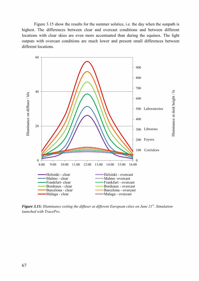
67

Figure 3.15 show the results for the summer solstice, i.e. the day when the sunpath is highest. The differences between clear and overcast conditions and between different locations with clear skies are even more accentuated than during the equinox. The light outputs with overcast conditions are much lower and present small differences between different locations.

Figure 3.15: Illuminance exiting the diffuser at different European cities on June 21st. Simulation launched with TracePro.

0

100

200

300

400

500

600

700

800

900

0

20

40

60

8:00 9:00 10:00 11:00 12:00 13:00 14:00 15:00 16:00

Illum

inan

ce a

t des

k he

ight

/ lx

Illum

inan

ce o

n di

ffuse

r / k

lx

Helsinki - clear Helsinki - overcastMalmo - clear Malmo -overcastFrankfurt- clear Frankfurt - overcastBordeaux - clear Bordeaux - overcastBarcelona - clear Barcelona - overcastMalaga - clear Malaga - overcast

Laboratories

Libraries

Foyers

Corridors

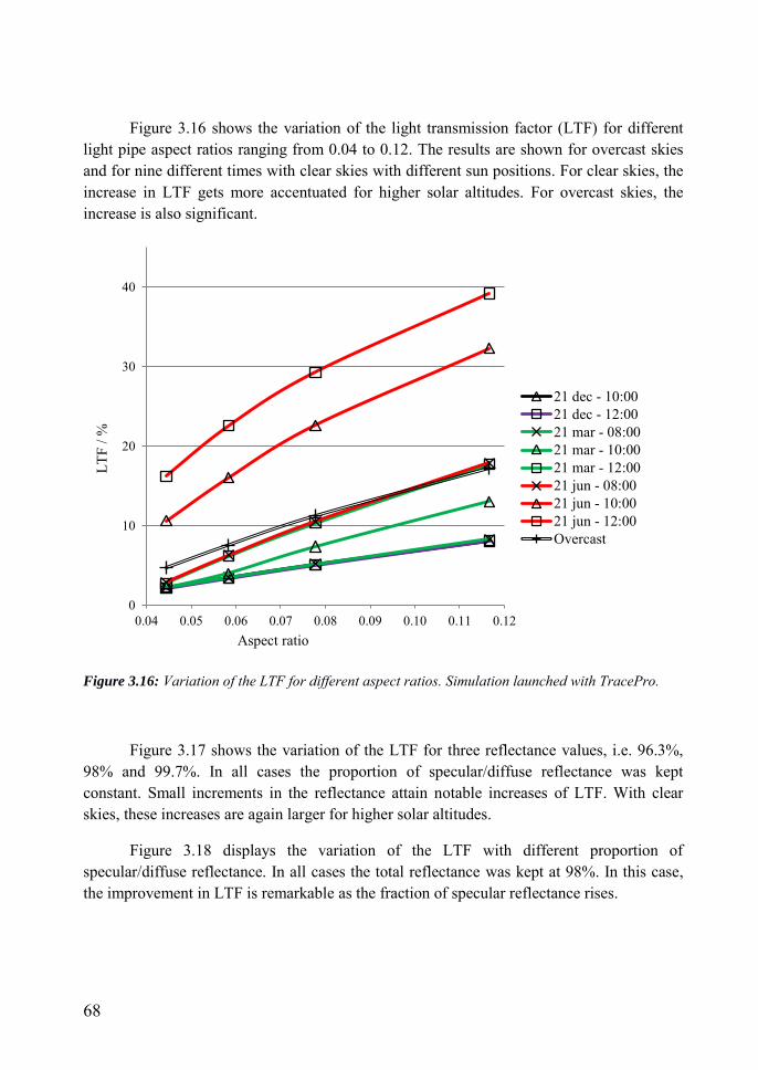
68

Figure 3.16 shows the variation of the light transmission factor (LTF) for different light pipe aspect ratios ranging from 0.04 to 0.12. The results are shown for overcast skies and for nine different times with clear skies with different sun positions. For clear skies, the increase in LTF gets more accentuated for higher solar altitudes. For overcast skies, the increase is also significant.

Figure 3.16: Variation of the LTF for different aspect ratios. Simulation launched with TracePro.

Figure 3.17 shows the variation of the LTF for three reflectance values, i.e. 96.3%, 98% and 99.7%. In all cases the proportion of specular/diffuse reflectance was kept constant. Small increments in the reflectance attain notable increases of LTF. With clear skies, these increases are again larger for higher solar altitudes.

Figure 3.18 displays the variation of the LTF with different proportion of specular/diffuse reflectance. In all cases the total reflectance was kept at 98%. In this case, the improvement in LTF is remarkable as the fraction of specular reflectance rises.

0

10

20

30

40

0.04 0.05 0.06 0.07 0.08 0.09 0.10 0.11 0.12

LTF

/ %

Aspect ratio

21 dec - 10:0021 dec - 12:0021 mar - 08:0021 mar - 10:0021 mar - 12:0021 jun - 08:0021 jun - 10:0021 jun - 12:00Overcast

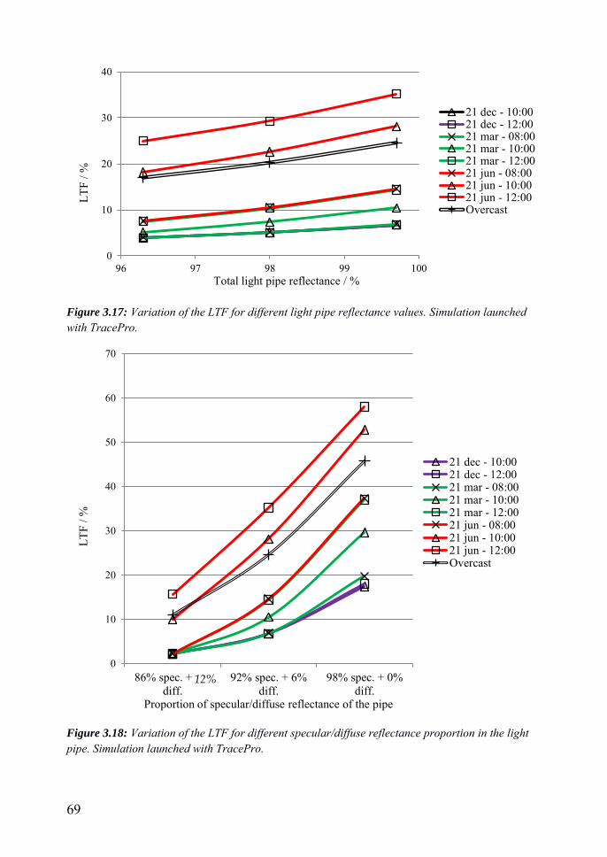
69

Figure 3.17: Variation of the LTF for different light pipe reflectance values. Simulation launched with TracePro.

Figure 3.18: Variation of the LTF for different specular/diffuse reflectance proportion in the light pipe. Simulation launched with TracePro.

0

10

20

30

40

96 97 98 99 100

LTF

/ %

Total light pipe reflectance / %

21 dec - 10:0021 dec - 12:0021 mar - 08:0021 mar - 10:0021 mar - 12:0021 jun - 08:0021 jun - 10:0021 jun - 12:00Overcast

0

10

20

30

40

50

60

70

86% spec. + 6%diff.

92% spec. + 6%diff.

98% spec. + 0%diff.

LTF

/ %

Proportion of specular/diffuse reflectance of the pipe

21 dec - 10:0021 dec - 12:0021 mar - 08:0021 mar - 10:0021 mar - 12:0021 jun - 08:0021 jun - 10:0021 jun - 12:00Overcast

12%

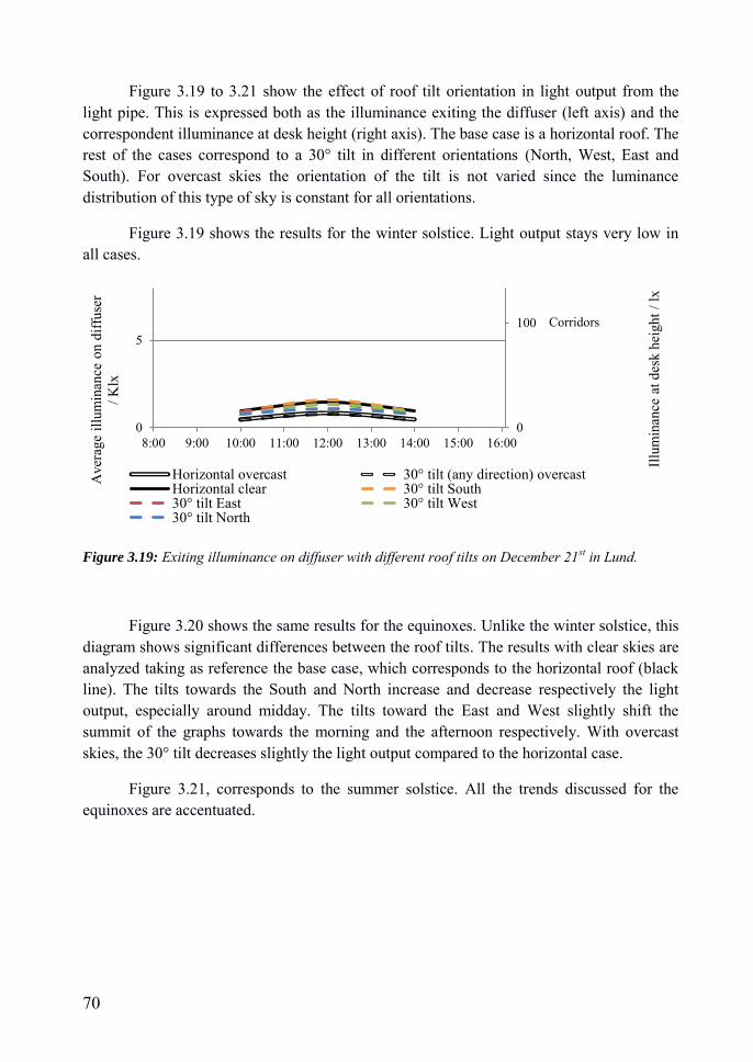
70

Figure 3.19 to 3.21 show the effect of roof tilt orientation in light output from the light pipe. This is expressed both as the illuminance exiting the diffuser (left axis) and the correspondent illuminance at desk height (right axis). The base case is a horizontal roof. The rest of the cases correspond to a 30° tilt in different orientations (North, West, East and South). For overcast skies the orientation of the tilt is not varied since the luminance distribution of this type of sky is constant for all orientations.

Figure 3.19 shows the results for the winter solstice. Light output stays very low in all cases.

Figure 3.19: Exiting illuminance on diffuser with different roof tilts on December 21st in Lund.

Figure 3.20 shows the same results for the equinoxes. Unlike the winter solstice, this diagram shows significant differences between the roof tilts. The results with clear skies are analyzed taking as reference the base case, which corresponds to the horizontal roof (black line). The tilts towards the South and North increase and decrease respectively the light output, especially around midday. The tilts toward the East and West slightly shift the summit of the graphs towards the morning and the afternoon respectively. With overcast skies, the 30° tilt decreases slightly the light output compared to the horizontal case.

Figure 3.21, corresponds to the summer solstice. All the trends discussed for the equinoxes are accentuated.

0

100

0

5

8:00 9:00 10:00 11:00 12:00 13:00 14:00 15:00 16:00

Illum

inan

ce a

t des

k he

ight

/ lx

Ave

rage

illu

min

ance

on

diffu

ser

/ Klx

Horizontal overcast 30° tilt (any direction) overcastHorizontal clear 30° tilt South30° tilt East 30° tilt West30° tilt North

Corridors

71

Figure 3.20: Exiting illuminance on diffuser with different roof tilts on March/September 21st in Lund.

0

100

200

0

10

8:00 9:00 10:00 11:00 12:00 13:00 14:00 15:00 16:00

Illum

inan

ce a

t des

k he

ight

/ lx

Ave

rage

illu

min

ance

on

diffu

ser /

Klx

Horizontal overcast 30° tilt (any direction) overcastHorizontal clear 30° tilt South30° tilt East 30° tilt West30° tilt North

Foyers

Corridors

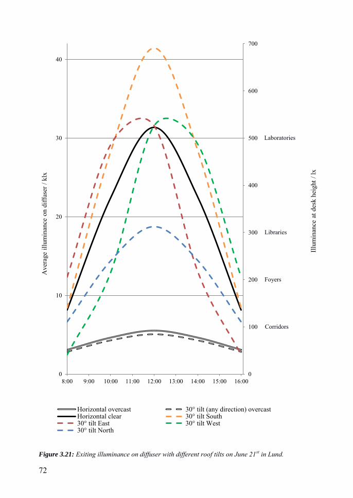
72

Figure 3.21: Exiting illuminance on diffuser with different roof tilts on June 21st in Lund.

0

100

200

300

400

500

600

700

0

10

20

30

40

8:00 9:00 10:00 11:00 12:00 13:00 14:00 15:00 16:00

Illum

inan

ce a

t des

k he

ight

/ lx

Ave

rage

illu

min

ance

on

diffu

ser /

klx

Horizontal overcast 30° tilt (any direction) overcastHorizontal clear 30° tilt South30° tilt East 30° tilt West30° tilt North

Laboratories

Libraries

Foyers

Corridors

73

4 Discussion

4.1 Evaluation of the simulation method

Variability of the measurements

The results are different for clear and overcast skies which is why these two sky types are discussed separately. Figures 3.1 to 3.4 display the discrepancy of simulated versus measured illuminance on each of the four sensors with overcast skies. Figures 3.5 to 3.8 show the same information for clear skies. The closer the crosses are to the diagonal line the lower the discrepancy.

With overcast skies illuminance levels strongly depend on the composition of the cloud layers, which makes the readings more variable and difficult to predict than in the case of clear skies. Figure 3.9 displays the absolute average deviation of consecutive measurements per sensor and sky type. It was calculated to give an idea of how much the illuminance in each of the sensors varies between the three measurements considered at each time. According figure 3.9, the illuminance variability is 2 to 5 times larger for overcast skies than for clear skies. These fluctuations between measurements are also illustrated by the broad spread of the crosses in Figures 3.1 to 3.4. In spite of this large variability, the average of the measurements follows the same trend as the simulated values.

Clear skies are more stable, except during the sunrise or the sunset, when the illuminance varies more rapidly. This is why times corresponding to sunrise or sunset moments, CL2 and CL5, were excluded in the calculation of the average AAD.

A good way to get rid of this uncertainty caused by the sky simulation is he use of HDR images from the actual simulated sky. This technique was previously explained in section 2.1. It can be used for any sky type, including intermediate skies.

Figure 3.9 also shows the importance of the sensor position in relation to the light pipe diffuser. “A” sensors (1A and 2A) are those located between two light pipes. The light levels on these sensors are much more volatile than on “B” sensors (1B and 2B), which are those located right below a light pipe. This is true both for overcast and clear skies, 2.5 times higher and 0.5-1.5 higher respectively. This different variability of light depending on the sensor position has different causes with each sky type.

With overcast skies, the low illuminance levels reaching the “A” sensors (5 to 30 lx) are in the same order of magnitude as the error margin of the sensors. This accentuated the variability of the sensor readings.

In the case of clear skies, the difference between “A” and “B” sensors can be related to the shape of the light beam from light pipes created by direct sun. Figure 4.1 shows a ring of light on the floor produced by sunlight transmitted through a light pipe. The size of this ring is very sensitive to variations in sun position, as shown in Figure 4.2. Small inaccuracies in the model or in the simulation of the sun position could have caused a different ring pattern. This was estimated to be a leading cause of the higher light variability on “A” sensors with clear skies.

74

This demonstrates the convenience of locating the sensors below a light pipe diffuser to reduce the variability of the measurements.

Figure 4.1: example of an illuminance distribution produced on the floor by direct sunlight thought a light pipe.

Figure 4.2: diagram showing how small a small variation of the solar angle can have a significant impact in the light reaching the sensor.

75

Correspondence between measurements and simulation results

The measured and the simulated values were also compared numerically (Table 3.1), using as measurement value the average of the three measurements considered at each time. With this comparison method overcast skies present a lower discrepancy than clear skies in all sensors.

It is important to acknowledge the sources of error before judging the discrepancies between measured and simulated values. In this case the accumulation of sources of error was estimated produce a total error of about ±20%. In view of this, relative discrepancies within those values can be considered accurate. With overcast skies in 85% of the cases the simulation values differed <20% from the average of the measurements and in 42% of the cases for clear skies. According to these results, overcast conditions were more accurately simulated than clear sky conditions.

With clear skies there is a distinct growing error trend as the illuminance gets higher in three of the four sensors (figures 3.5 to 3.8). The illuminance levels are determined essentially by the solar altitude, especially with clear skies. In this case the range of solar altitudes is limited to values lower than 30 degrees. This is due to the fact that the measurements were taken during winter months. Times with higher solar altitudes during summer should also be assessed to confirm this trend.

Taking a closer look at the figures a further distinction can be made. Sensors 1A and 2A present a tendency to overestimate the measurements while in sensor 2B the tendency is to underestimate them. The fourth sensor (1B) follows approximately the trend of the measurements. Otherwise said, the simulations for stable 1 (Velux light pipes) matches the measurements in one sensor and overestimates them in the other one. In stable 2 (Solatube light pipes) one sensor overestimates and the other one underestimates them.

In stable 1 all the elements of the light pipes were correctly characterized, including the BSDF of the diffuser. The leading cause of the overestimation of the illuminance values in sensor 1A is an incorrect representation of sunlight. Sensor 1A is lit by sunlight while sensor 1B (the one were the simulation matched the measurements) is only lit by sky-light. Figure 4.4 shows how direct sunlight is shaded from the collector of light pipe three, located on the North pitch of the roof. Sensor 1B is lit by this light pipe. On the other hand, sensor 1A (the one that presents an overestimation trend) is located between light pipes one and two, which receive direct sunlight. This leads to the conclusion that the direct sun contribution was overestimated and sky light was correctly simulated. The method used to estimate the solar constant (pages 39-40) should thus be reexamined. The use of HDR images of the simulated skies would also solve this problem.

In stable 2, the opposite trends (overestimation and underestimation) in the sensors can be explained by the absence of goniophotometric measurements for the Solatube dome collector. This element is an Optical Redirecting System that requires this type of information to take in consideration its light bending properties. Figure 4.3 illustrates how the sunrays are redirected into de pipe at lower angles reaching the area around “B”. The simulated rays (dotted line) are not bent in the collector and reach the room at lower angles, producing an overestimation in “A” and an underestimation in “B”. Theoretically, the trends would have been similar to the one of sensor 1A in Stable 1 (overestimation due to sunlight) if it had been possible to simulate the collector dome’s light bending properties by including its goniophotometric characterization.

76

The Solatube light pipes analyzed show higher light output than the Velux ones. This is due to many factors: higher light pipe reflectance, higher specular reflectance, higher transmittance in the collector and the diffuser, the innovative dome, etc. The large differences between sensors 1B and 2B are to a high extent cause by the fact that the Velux collector was exposed to direct sunlight while the Velux collector was shaded by the roof. It was also noted that the light redirecting properties of the Solatube dome collector result in a narrower light beam than in the Velux light pipes.

Figure 4.3: diagram showing how the lack of the characterization of the dome collector light bending properties causes overestimation in “A” and underestimation in “B”.

Figure 4.4: Sensor 1A is reached by sunlight, sensor 1B is not.

77

4.2 Parametric study

Six design parameters were varied in this parametric study: location, pipe length and diameter, total pipe reflectance, proportion of specular/diffuser light pipe reflectance and roof pitch. The results were grouped together into four categories: solar altitude, light pipe aspect ratio, light pipe reflectance and roof pitch. Each of these categories is discussed separately below:

4.2.1 Solar altitude

From the categories analyzed, solar altitude is the one with the highest impact on the light output from the light pipes, especially for clear skies. The results displayed in Figures 3.10 to 3.12 indicate that both the LTF and the absolute illuminance values increases rapidly as solar altitude is increased with for clear skies (Figures 3.10 and 3.12).

The simulation method overestimates direct sunlight in clear skies as the solar altitude is increased. Figure 3.11 displays the trend lines for the measurements and the simulation results for sensor 1B in the pig stables. Sensor 1B was considered the most suitable to be used as reference for the parametric study because of its similarities with the parametric study model, i.e. it is below a light pipe equipped with a flat collector. This figure shows that, although they are not identical, the trend line of the measurements and that of the simulation values show a similar exponential growth. Therefore, even though the results of this parametric study will not be totally accurate, the trends it shows are trustworthy.

The large increase of light output with increasing solar altitude is not surprising as this parameter affects five of the six factors for clear skies showed Table 2.7. Unfortunately, solar altitude is given by the location and cannot thus be modified. However, it might be possible to improve LTF for lower solar altitudes by tilting or bending the pipe towards the South.

The results indicate much lower illuminance output for overcast conditions. According to Figure 3.12 the percentage of light that goes thought the light pipe (LTF) with overcast skies stays constant as the solar altitude is varied. This indicates that the slight illuminance growth for overcast skies shown in Figure 3.10 is entirely caused by the growth in GHI (factor 1 in Table 2.7). This is due to the fact that the illuminance distribution of overcast skies is constant for all sun positions.

According to Figure 3.10, simple light pipes with clear sky conditions could provide sufficient light for corridors (for solar altitudes >30º), foyers (>40º), libraries (>45º) and even laboratories (>60º). The corresponding values with overcast conditions, however, barely attain corridor levels, even for high solar altitudes. It should be noted that these figures are somewhat overestimated.

The difference in light output from the light pipe between overcast and clear skies is confirmed by the pig stables illuminance measurements. In times CL4 (clear sky) and OC1 (overcast sky) the sun was approximately in the same position in the sky. Sensors 1B and 2B are both located light below a light pipe. The light pipe above 1B is shaded from sunlight by the roof while the one above 2B can receive sunlight.

78

The difference in light reaching sensor 2B in CL4 (clear sky) is 280% higher than in OC1 (overcast sky), and only 8% higher for sensor 1B. This proves the large effect of direct sunlight in light pipe output.

Solar altitude is linked to latitude. The impact of latitude on light pipe output was assessed for different cities in Europe. Figures 3.13 to 3.15 show the results of the simulations on the equinoxes and solstices at six different locations, from Hensinki (60°N) to Malaga (37°N).

The results show that, with clear skies, latitude has a very big impact on light pipe performance. The results for Helsinki and Malaga are compared next. During the winter solstice (Figure 3.13) only corridor light levels are reached at midday in Malaga, while in Helsinki light output that tops out at 20 lx. During the equinox (Figure 3.14) Helsinki still does not reach corridor levels, while Malaga exceeds it during 2h55’. During the summer solstice Helsinki reaches library levels for 1h55’ and corridor levels for 3h50’. The same values for Malaga are once again much higher, 5h20’ and 7h55’ accordingly. As in can be seen from these figures, latitude has a big impact on light pipe output with clear sky conditions.

The same results for overcast skies show that the illuminance levels reached are much lower for all locations and that the influence of latitude is less accentuated. Corridor light levels are only attained on the summer solstice, during 1h40’ in Helsinki and 2h15’ in Malaga.

Therefore, light pipes are more effective when used in Southern European countries than in Scandinavian countries for two reasons: solar altitude and sky clearness (direct sunlight occurs during around 2,000 hours in the Southern Europe and only about 1,000 hours in the Scandinavian countries).

These findings reveal that light pipes performance is reduced significantly with low solar altitudes and overcast skies. Unfortunately, this makes them unsuitable to improve daylighting in Scandinavian countries during winter. Fiberoptic sun tracking systems might be more suitable for this context (Oh, et al., 2012). These systems only work with direct sunlight but, unlike light pipes, they can effectively collect sunlight from low solar altitudes.

4.2.2 Aspect ratio

The impact of light pipe aspect ratio in the light output is significant, although not as much as that of the solar altitude. However, unlike solar altitude, this parameter can be manipulated by the designer. Aspect ratio determines the amount of light bounces in the pipe. According to Figure 3.16 the LTF grows notably as the aspect ratio is increased. It grows faster for lower aspect ratios and tends to stabilize as the aspect value gets larger. For clear skies, this trend is more pronounced as the solar altitude is increased. Increasing the aspect ratio from 0.1 to 0.06 led to 11.5% additional light on the summer solstice at midday and only 6% on the winter solstice at midday. The increase of LFT as a function of light pipe ratio is not dependent on solar altitude for overcast skies. Increasing the aspect ratio from 0.1 to 0.06 with overcast skies produced an increase of 4.5% in LTF.

79

4.2.3 Light pipe illuminance

The reflectance of the light pipe and, more specifically, the specular reflectance have a drastic effect on the percentage of light that goes through the light pipe (LTF).

Figure 3.17 shows the LTF of the light pipe as a function of the light pipe reflectance (values between 96% and 99.7%). It presents eight different times with clear skies and only one for overcast conditions (LTF is independent from the sun position for overcast skies). In this case, an increase of about 1% to 3% LTF can be observed for each additional percentage point in reflectance, the highest increases corresponding to higher solar altitudes.

Figure 3.18 shows the result of varying the specular reflectance keeping constant the total reflectance. The light pipe LTF increased 1.5% to 4% for each percentage point that was transferred from diffuse to specular reflectance. This proves the importance of improving the pipe specular reflectance to attain better light outputs from light pipes.

4.2.4 Roof tilt orientation

The impact of roof tilt on light pipe output is not negligible during most of the year. This impact is positive for South tilts and negative for North tilts. West and East tilts affect the distribution of the output throughout the day.

Figures 3.19 to 3.21 show the variation of illuminance on the diffuser for different tilts on December 21st, March 21st and June 21st respectively, both for overcast and clear conditions. In the case of overcast sky two options were included: horizontal and 30° tilt. Orientation is not relevant in this case because the illuminance distribution is constant for all orientations. In the case of clear skies the cases analyzed are: horizontal and 30° tilt towards South, North, West and East.

Figure 3.19 show the variations on the winter solstice in Lund. Illuminance levels at desk height tops at 10 to 30 lux at desk height, which is below the reference value for corridors (100lx). These low levels are due to very low solar altitudes below 11°. The differences between different roof tilts are low as well.

In the other two dates considered (March 21st and June 21st) the differences with clear skies are significant. A tilt of 30° to the South increased the peak of the illuminance curve at midday by 52% and 32% for March and June respectively. On the other hand, the illuminance peak was reduced by 71% and 40% when the roof was tilted 30° to the North. The effect of the tilts on the illuminance is highest around midday and decreases towards the morning and evening for both the South and North tilts. In the case of West and East orientations the illuminance peak shifted towards the afternoon and the morning respectively 30 minutes in the case on March 21st and 40 minutes in the case of June 21st. The peak increased slightly by 0.3% and 4% correspondingly. These results show general trends, it is advised to assess the best orientation and tilt angle with clear skies for each case and location by running a small assessment using the forward raytracing system.

80

For overcast skies the peaks were slightly reduced by 2% and 8% for March 21st and June 21st respectively. It can be concluded from this that, with overcast skies, horizontal roofs are optimum for light pipes.

81

5 Conclusions

5.1 Forward raytracing as simulation method for light pipes

In this study a forward raytracing simulation method was used to simulate light output from light pipes. The simulation results with overcast skies presented an acceptable accuracy, with discrepancies between the simulated value and the average of three measurements <30% in 100% of the cases, <20% in 85% of the cases and <10% in 40% of the cases. The discrepancies of the forward raytracing method with clear skies were higher: <30% discrepancy in 67% of the cases, <20% in 42% of the cases and <10% in 17% of the cases. The higher discrepancies with clear skies are due to the overestimation of sunlight and the absence of BSDF for the dome collectors.

These are some recommendations to simulate light pipes output using the forward raytracing method:

- The specular and the diffuse reflectance of the pipes needs to be described with accuracy, since small inaccuracies can produce significant errors.

- Goniophotometric properties of all the ORS in the light pipes need to be described by BSDF, especially for simulations with clear skies. This information should be provided by the manufacturers. The goniophotometric definition of the diffuser affects the distribution of the light output, while the goniophotometric definition of the collector also affects the amount of light transmitted by the light pipe.

- GHI can vary largely with overcast skies. A factor to take in consideration the discrepancy of measured and simulated GHI needs to be calculated and used to weight the results.

Another additional measure that can help to improve the accuracy of the results is the use of HDR images of the simulated skies instead of generic sky models. This method also allows the simulation of intermediate skies.

The illuminance values produced by light pipes fluctuate significantly over short periods, especially with overcast skies. Some measures that can be taken to limit this variability are:

- Placing the sensors below the light pipe diffuser.

- Considering several consecutive measurements.

- Not considering very low luminance values in the same order of magnitude as the sensor error margin.

- Not considering dusk or dawn because light levels vary rapidly during these moments of the day.

- Simulating and measuring the outdoors GHI at the specific moment assessed to obtain a factor to weigh the results. This is especially useful with overcast skies (GHI can vary largely due to the characteristics of the cloud layers).

82

5.2 Guidelines for light pipe design

Solar altitude and sky clearness are crucial factors for the light pipe performance. Light pipes perform better in sunny climates at low to mid latitudes with higher solar altitudes like Southern Europe. The performance is not as good in cloudy climates at high latitudes, like Scandinavian countries. They also work better in summer, when the sun is higher than in winter. Some methods to improve LTF for low solar altitudes are: bending or tilting the pipe, increasing the aspect ratio, improving the pipe specular reflectance, tilting the collector to the South and using ORS in the collector.

With clear skies, a simple light pipe requires a solar altitude of 30° to reach corridor light levels, 40° for foyers, 45° for libraries and 60° for laboratories. These are guide values; the actual value varies for each specific light pipe and location.

With overcast skies, the output from light pipes is lower; it can hardly reach corridor light levels. The light output is less affected by solar altitude than in the case with clear skies because the illuminance distribution is similar for all overcast skies.

The light pipe aspect ratio has a significant impact in LTF, as it determines the number of light bounces in the pipe. In the Scandinavian context, a high aspect ratio above 1/15 is recommended to make up for low solar altitudes.

The reflectance of the pipe and, more precisely, the specular reflectance have a drastic influence on the light pipe LTF. In the case analyzed in this parametric study each additional percentage point in reflectance produced an increase of one to three points in the LTF. Every percentage point that was transferred from diffuse to specular reflectance led to an increase of 1.5% to 4% in the light output.

South roof tilts increase significantly the luminance output around midday. North tilts should be avoided as they can considerably reduce it. West and East tilts are advisable if they serve spaces to be used rather during the afternoon or during the morning respectively. These are just general guidelines. A small assessment should be carried out to find out the optimum tilt angle orientation for each particular project and location.

83

5.3 Future research

A future research will be done as a continuation of this master thesis with two goals: solving the problem of overestimation of direct sunlight for higher solar altitudes and creating a methodology to apply forward raytracing to annual calculations.

The results of this project show that the methodology used to simulate output from light pipes caused a non-negligible overestimation of direct sunlight for solar altitudes over 30 degrees. The continuation of this project will address this issue to give it a solution.

Once the simulations work correctly, a methodology will be created to apply the methodology of forward raytracing to annual climate based calculations. This would permit to predict yearly savings of electric light produced by light pipes for each specific case and location. In turn, this would allow the inclusion of light pipes in environmental certification schemes for buildings, such as LEED or BREEAM.

Some other parameters to improve the light pipes performance for low angle sunlight could be added to the parametric study, such as the tilt of the pipe or the inclusion of different ORS in the collector.

84

6 References

Akashi, Y., Tanabe, Y., Akashi, I., & Mukai, K. (2000). Effect of sparkling

luminous elements on the overall brightness impression: A pilot study. Lighting Research and Technology, 32, 19–26.

Ashkenazy, T., Einat, H., & Kronfeld-Schor, N. (2009). Effects of bright light treatment on depression- and anxiety-like behaviors of diurnal rodents maintained on a short daylight schedule. Behavioral Brain Research, 201(2), 343–346.

Danny, H., Ernest, K., Cheung, K., & Tam, C. (2010). An analysis of light-pipe system via full-scale measurements. Applied Energy, 87, 799–805.

De Boer, J. (2003). Incorporation of numerical goniophotometry into daylighting design . Proceedings of CISBAT 2003: Innovation in Building Envelopes and Environmental Systems, (pp. 229–234). Lausanne, Switzerland.

Dehoff, P. (2002). The impact of changing light on the well-being of people at work. In Proceedings of Right Light, 5 (pp. 374-351).

Dutton, S., & Shao, L. (2007). Raytracing simulation for predicting light pipe transmittance. International Journal of Low Carbon Technologies, 2(4), 339-358.

Edmonds, I., Moore, G., Smith, G., & Swift, P. (1995). Daylighting enhancement with light pipes coupled to laser-cut light-deflecting panels. Lighting Research & Technology, 27, 27–35.

Energy Information Administration. (2007). Intenational emissions data: Energy Related Carbon Emissions. Available from http://www.eia.doe.gov/environmental.html.

Eurostat. (2009). European Commission - Eurostat. Available from: http://epp.eurostat.ec.europa.eu/portal/page/portal/eurostat/home/.

Farrel, A., Norton, B., & Kennedy, D. (2004). Lightpipe daylight simulation modeling using Radiance backward and and forward raytracing methods: A comparison with monitored data for commercial lightpipes in Ireland. Retrieved March 26, 2014, from Third International Radiance Workshop, École d’ingénieurs et d’architectes de Fribourg, Switwerland: http://www.radiance-online.org/radiance-workshop3

Figueiro, G. M. (2002). Daylight and Productivity - A Field Study. Proceedings of 2002 ACEEE Summer Study on Energy Efficiency in Buildings. Washinngton DC: American Council for an Energy-efficient Economy.

Harteb Puleo, S., & Leslie, R. (1991). Some effects of sequential experience of windows in human response. Journal of the IES, 20(1), 91-99.

Heschong Mahone Group. (2003). Daylight and Retail Sales. Fair Oaks, California: Heschong Mahone Group.

Hore-Lacy, I. (2003). Nuclear Electricity, 7th edition. UK: Uranium Information Centre - Australia and World Nuclear Association.

85

IESNA. (1999). Recommended practice of daylighting. Daylighting Committee. Inanici, M. (2010). Evaluation of high dynamic range image based sky models in

lighting simulation. Seattle: University of Washington, Department of Architecture.

International Energy Agency. (2001). Monitoring Procedures for the Assessment of Daylighting Performance of Buildings. A Report of IEA SHC Task 21 / ECBCS Annex 29.

International Energy Agency. (2006). Light's labour cost. France: IEA Publications. Jenkins, D., Munner, T., & Kubie, J. (2005). A design tool for predicting the

performances of light pipes. Energy and Building, 37, 485–492. Jenkins, T., & Muneer. (2003). Modelling light-pipe performances – a natural

daylighting solution. Building and Environment, 38, 965 – 972. Kjellsson, E. (2002). Solar heating systems for electricity heated houses. Report

number U02:86. Vattenfall AB. Kocifaj, M. (2009). Efficient tubular light guide with two-component glazing with

Lambertian diffuser and clear glass. Applied Energy, 86, 1031–1036. Kocifaj, M., Darula, S., & Kittler, R. (2007). HOLIGILM: Hollow light guide

interior illumination method – An analytic calculation approach for cylindrical light-tubes. Solar Energy, 82, 247–259.

Kohler, C. (2010). NFRC presentation. Retrieved January 21, 2014, from Initial summary of round robin tvis measurements for tubular daylighting devices (TDD).: www.nfrc.org/documents/ComplexProductVTpresentation_April2010ss.pdf

Kolås, T. (2013). Performance of Daylight Redirecting Venetial Blinds for Sidelighted Spaces at High Latitudes, Performance analysed by forward raytracing simulations with the software TracePro. Thesis for the degree of Philosophiae Doctor, Trondheim, Norwegian University of Science and Technology, Faculty of Architecture and Fine Art, Department of Architectural Design, Form and Colour.

Kómar, L., & Darula, S. (2012). Determination of the light tube efficiency for selected overcast sky types. Solar Energy Volume 86 (1), 157–163.

Kómar, S., & Darula. (2011). Determination of the light tube efficiency for selected overcast sky types. Solar Energy, 86, 157–163.

Lambda Research Corporation. (2014). TracePro® User Manual, Release 7.4. Lo Verso, V., Pellegrino, A., & Serra, V. (2011). Light transmission efficiency of

daylight guidance systems: An assessment approach based on simulations and measurements in a sun/sky simulator. Solar Energy, 85, 2789–2801.

Mardaljevic, J., Heschong, L., & Lee, E. (2009). Daylight metrics and energy savings. Lighting Research & Technology, 41, 261-283.

McKinsey. ( 2008). The carbon productivity challenge: Curbing climate change and sustaining economic growth. McKinsey global institute. http://www.mckinsey.com/mgi/publications/Carbon_Productivity/index.asp. .

86

Mohelníková, F., & Vajkay, J. (2009). Study of tubular light guides illuminance simulations. Leukos, 5 (4), 267–277.

Mohelnikova, J. (2009). Tubular light guide evaluation. Building and Environment, 44, 2193–2200.

Murdoch, J. (1985). Illumination Engineering – from Edison´s lamp to the laser. Macmillan Pub. Co.

Nair, M., Ramamurthy, K., & Ganesan, A. (2014). Classification of indoor daylight enhancement systems. Lighting Research and Technology, 46, 245–267.

National Fenestration Rating Council. (2008). Complex product vt rating project monitoring. Retrieved July 21, 2012, from www.nfrc.org/complexprodvtrfpbrtg.aspx

Nilsson, A. (2012). Daylighting Systems: Development of Techniques for Optical Characterization and Performance Evaluation. Uppsala: Acta Universitatis Upsaliensis. Digital Comprehensive Summaries of Uppsala Dissertations from the Faculty of Science and Technology.

Robertson, A., Hedges, R., & Rideout, N. (2010). Optimization and design of ducted daylight systems. Lighting Research & Technology, 42, 161–181.

S Traberg-Broup, K. G. (2005). Effektiv belysning i kontor og erhervbyggeri, En undergöelse in ni kontorbygninger. Report SBI 2005:06. Horsholm, Denmark: Statens Byggeforskningsinstitut.

Solatube International, Inc. (n.d.). Retrieved February 10, 2014, from www.solatube.com/commercial/product-catalog/brighten-up-series/index.php

Stern, N. (2007). Stern review: The Economics of Climate change. UK: HM Treasury.

Swedish Energy Agency. (2012). Energy in Sweden 2012. Available from: www.energimyndigheten.se/Global/Engelska/Facts%20and%20figures/Energy_in_sweden_2012.pdf.

Swift, P. (2010). Splayed mirror light pipes. Solar Energy, 84 , 160–165. Swift, P., Lawlor, R., Smith, G., & Gentle, A. (2008). Rectangular section mirror

light pipes. Solar Energy Materials & Solar Cells 92, 969–975. Thanachareonkit, A., Scartezzini, J.-L., & Andersen, M. (2005). Comparing

daylighting performance assessment of buildings in scale models and test modules. Solar Energy, 79 (2), 168–182.

The European Database of Daylight and Solar Radiation. (n.d.). Retrieved April 23, 2014, from The European Database of Daylight and Solar Radiation. http://www.satel-light.com.

TracePro®. (n.d.). TracePro® website. Retrieved March 16, 2014, from http://www.lambdares.com/tracepro

Tregenza, P., & Wilson, M. (2011). Daylighting: Architecture and Lighting Design. Routledge.

Urge-Vorsatz, Novikova, & Levine. (2008). Non-residential buildings for mitigating climate change: Summary of the findings of the Intergovernmental Panel on

87

Climate Change. Improving Energy Efficiciency in Commercial Buildings Conference. Frankfurt.

Zhang, T., & Muneer. (2000). Mathematical model for the performance of light-pipes. Lighting Research and Technology, 32, 141-46.

Zhang, X., Muneer, T., & Kubie, J. (2002). A design guide for performance assessment of solar light-pipes. Lighting Research and Technology, 34, 149.

Cover picture obtained from the Solatube website with the consent of the company.

88

Appendix A: Simulation methodology evaluation detailed results

This appendix presents detailed data used to calculate both the measured and the simulated results in each of the eleven times considered. The variation between measurements and simulation results is presented as well.

Three consecutive measurements (5 in the case of OC1) were considered for each of the times. Each of these measurements is the averaged value for a six minute span. Tables A.1 to A.8 display at the top part the list of measurements considered, then the average of these three values and then the final measured value, named ‘Average measured illuminance’. This last value is calculated by multiplying the average of the measurements by its respective Sensor Dirt Factor.

The lower part of the table shows the simulation results. These are calculated for each of the light pipes and then summed up for each sensor. The contributions from light pipes that are too far from a sensor to be significant are dismissed. The sum is then multiplied by a factor that takes into account the difference between the measured and the simulated GHI called GHI factor. Finally, 5% is deduced from the result to account for dirt accumulation in the light pipe. The resulting value is called ‘simulated illuminance’.

The discrepancies between the Simulated illuminance and the Average measured illuminance are calculated and expressed as a percentage according to the following formula:

Tables A.1 to A.11 show these detailed data for each of the eleven times considered to compare the measurements and the simulation results.

89

Table A.1: Detailed measured and simulated illuminance data in moment OC1 (overcast, Kt =0.92).

Velux Solatube GHI

Sens.1A Sens.1B Sens.2A Sens.2B

Ons

ite m

easu

rem

ents

2014/02/11 14:00, (lux) 7.75 65.59 39.05 79.23 6314.27

2014/02/11 14:06, (lux) 15.35 60.37 33.33 50.6 5057.80

2014/02/11 14:12, (lux) 20.17 71.48 16.33 69.17 5975.01

2014/02/11 14:18, (lux) 10.1 75.94 28.15 83.2 6557.67

2014/02/11 14:24, (lux) 5.051 50.35 20.15 60.26 5063.94

Average, (lux) 11.68 64.75 27.40 68.49 5793.74

SDF (Sensor Dirt Factor) 0.00 0.00 0.00 0.00

Average measured illum., (lux) 11.68 64.75 27.40 68.49

Sim

ulat

ion

Tra

cePr

o Light pipe 1, (lux) 15.12 - 24.35 - Light pipe 2, (lux) 1.44 0.64 5.09 2.14 Light pipe 3, (lux) - 52.86 - 74.42

Light pipe 4, (lux) - 0.37 - 2.29

Sum, (lux) 16.56 53.87 29.44 78.85

Simulated illuminance*, (lux) 13.98 45.47 24.85 66.55 6521.00 Relative discrepancy, (%) 19.6 -29.8 -9.3 -2.8

(*) GHI factor = 0.89 Light pipe dirt factor = 5%

Table A.2: Detailed measured and simulated illuminance data in moment OC2 (overcast, Kt = 1). Velux Solatube GHI

Sens.1A Sens.1B Sens.2A Sens.2B

Ons

ite m

easu

rem

ents

2014/02/19 16:06, (lux) 9.67 31.13 15.14 31.73 3466.87

2014/02/19 16:12, (lux) 8.42 26.87 8.86 25.19 2831.15

2014/02/19 16:18, (lux) 3.98 24.07 19.19 32.22 2897.66

Average, (lux) 7.36 27.36 14.40 29.71 3065.23

SDF (Sensor Dirt Factor) 1.21 1.15 1.23 1.13

Average measured illum., (lux) 8.87 31.44 17.65 33.66

Sim

ulat

ion

Tra

cePr

o Light pipe 1, (lux) 7.32 - 15.46 - Light pipe 2, (lux) 0.65 0.30 4.17 1.38 Light pipe 3, (lux) - 28.01 - 37.96

Light pipe 4, (lux) - 0.26 - 1.20

Sum, (lux) 7.97 28.57 19.63 40.54

Simulated illuminance*, (lux) 7.35 26.34 18.10 37.38 3158.10 Relative discrepancy, (%) -17.1 -16.2 2.6 11.1

(*) GHI factor = 0.97 Light pipe dirt factor = 5%

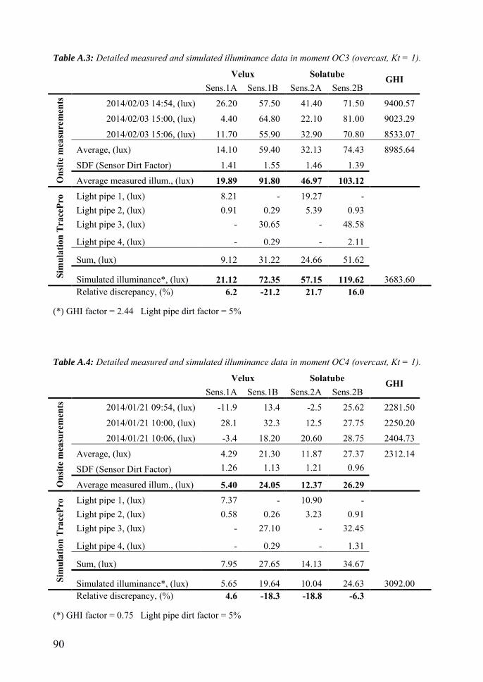
90

Table A.3: Detailed measured and simulated illuminance data in moment OC3 (overcast, Kt = 1). Velux Solatube GHI

Sens.1A Sens.1B Sens.2A Sens.2B

Ons

ite m

easu

rem

ents

2014/02/03 14:54, (lux) 26.20 57.50 41.40 71.50 9400.57

2014/02/03 15:00, (lux) 4.40 64.80 22.10 81.00 9023.29

2014/02/03 15:06, (lux) 11.70 55.90 32.90 70.80 8533.07

Average, (lux) 14.10 59.40 32.13 74.43 8985.64

SDF (Sensor Dirt Factor) 1.41 1.55 1.46 1.39

Average measured illum., (lux) 19.89 91.80 46.97 103.12

Sim

ulat

ion

Tra

cePr

o Light pipe 1, (lux) 8.21 - 19.27 - Light pipe 2, (lux) 0.91 0.29 5.39 0.93 Light pipe 3, (lux) - 30.65 - 48.58

Light pipe 4, (lux) - 0.29 - 2.11

Sum, (lux) 9.12 31.22 24.66 51.62

Simulated illuminance*, (lux) 21.12 72.35 57.15 119.62 3683.60 Relative discrepancy, (%) 6.2 -21.2 21.7 16.0

(*) GHI factor = 2.44 Light pipe dirt factor = 5%

Table A.4: Detailed measured and simulated illuminance data in moment OC4 (overcast, Kt = 1). Velux Solatube GHI

Sens.1A Sens.1B Sens.2A Sens.2B

Ons

ite m

easu

rem

ents

2014/01/21 09:54, (lux) -11.9 13.4 -2.5 25.62 2281.50

2014/01/21 10:00, (lux) 28.1 32.3 12.5 27.75 2250.20

2014/01/21 10:06, (lux) -3.4 18.20 20.60 28.75 2404.73

Average, (lux) 4.29 21.30 11.87 27.37 2312.14

SDF (Sensor Dirt Factor) 1.26 1.13 1.21 0.96

Average measured illum., (lux) 5.40 24.05 12.37 26.29

Sim

ulat

ion

Tra

cePr

o Light pipe 1, (lux) 7.37 - 10.90 - Light pipe 2, (lux) 0.58 0.26 3.23 0.91 Light pipe 3, (lux) - 27.10 - 32.45

Light pipe 4, (lux) - 0.29 - 1.31

Sum, (lux) 7.95 27.65 14.13 34.67

Simulated illuminance*, (lux) 5.65 19.64 10.04 24.63 3092.00 Relative discrepancy, (%) 4.6 -18.3 -18.8 -6.3

(*) GHI factor = 0.75 Light pipe dirt factor = 5%

91

Table A.5: Detailed measured and simulated illuminance data in moment OC5 (overcast, Kt = 1). Velux Solatube GHI

Sens.1A Sens.1B Sens.2A Sens.2B

Ons

ite m

easu

rem

ents

2014/01/01 11:54, (lux) 19.8 45.3 18.7 62.6 5798.64

2014/01/01 12:00, (lux) -10 42.4 27.7 56.14 5432.17

2014/01/01 12:06, (lux) 19.5 47.8 18.3 52.38 4432.54

Average, (lux) 9.77 45.17 21.57 57.04

SDF (Sensor Dirt Factor) 1.2 1.18 1.25 1.03

Average measured illum., (lux) 11.74 53.40 26.87 59.23 5221.13

Sim

ulat

ion

Tra

cePr

o Light pipe 1, (lux) 9.69 - 18.47 - Light pipe 2, (lux) 0.89 0.25 4.51 1.58 Light pipe 3, (lux) - 35.30 - 41.01

Light pipe 4, (lux) - 0.28 - 1.32

Sum, (lux) 10.58 35.82 22.98 43.91

Simulated illuminance*, (lux) 13.05 44.17 28.34 54.15 4022.40 Relative discrepancy, (%) 11.1 -17.3 5.5 -8.6

(*) GHI factor = 1.30 Light pipe dirt factor = 5%

Table A.6: Detailed measured and simulated illuminance data in moment CL1 (clear sky, Kt =0.14). Velux Solatube GHI

Sens.1A Sens.1B Sens.2A Sens.2B

Ons

ite m

easu

rem

ents

2014/02/04 11:54, (lux) 34.66 46.21 62.93 160.7 26712.82

2014/02/04 12:00, (lux) 34.92 53.6 63.81 156.7 26998.40

2014/02/04 12:06, (lux) 23.85 39.94 51.06 170.6 27016.01

Average, (lux) 31.14 46.58 59.27 162.67 26909.08

SDF (Sensor Dirt Factor) 1.43 1.55 1.46 1.39

Average measured illum., (lux) 44.57 71.99 86.63 225.37

Sim

ulat

ion

Tra

cePr

o Light pipe 1, (lux) 54.95 - 87.27 - Light pipe 2, (lux) 10.58 0.60 22.15 9.69 Light pipe 3, (lux) - 69.72 - 120.77

Light pipe 4, (lux) - 0.67 - 14.74

Sum, (lux) 65.53 70.99 109.41 145.20

Simulated illuminance*, (lux) 57.84 62.65 96.57 128.15 28963.00 Relative discrepancy, (%) 29.8 -13.0 11.5 -43.1

(*) GHI factor = 0.93 Light pipe dirt factor = 5%

92

Table A.7: Detailed measured and simulated illuminance data in moment CL2 (clear sky, Kt = 0). Velux Solatube GHI

Sens.1A Sens.1B Sens.2A Sens.2B

Ons

ite m

easu

rem

ents

2014/02/10 15:24, (lux) 22.17 34.89 46.11 136 18528.61

2014/02/10 15:30, (lux) 24.35 27.37 38.21 124.3 17083.08

2014/02/10 15:36, (lux) 30.19 34.43 19 124.8 15856.63

Average, (lux) 25.57 32.23 34.44 128.37 17156.11

SDF (Sensor Dirt Factor) 1.40 1.28 1.37 1.28

Average measured illum., (lux) 35.86 41.33 47.27 164.06

Sim

ulat

ion

Tra

cePr

o Light pipe 1, (lux) 38.87 - 55.03 - Light pipe 2, (lux) 5.46 1.84 21.04 17.69 Light pipe 3, (lux) - 39.33 - 137.98

Light pipe 4, (lux) - 0.62195 - 14.01

Sum, (lux) 44.33 41.79 76.07 169.68

Simulated illuminance*, (lux) 37.49 35.34 64.34 143.52 19270.00 Relative discrepancy, (%) 4.5 -14.5 36.1 -12.5

(*) GHI factor = 0.89 Light pipe dirt factor = 5%

Table A.8: Detailed measured and simulated illuminance data in moment CL3 (clear sky, Kt =0.01). Velux Solatube GHI

Sens.1A Sens.1B Sens.2A Sens.2B

Ons

ite m

easu

rem

ents

2014/02/10 12:54, (lux) 35.28 52.37 87.5 233.8 34949.83

2014/02/10 13:00, (lux) 42.09 47.46 87.5 217.4 34711.19

2014/02/10 13:06, (lux) 38.39 51.82 87.5 204.9 32669.05

Average, (lux) 38.59 50.55 87.50 218.70

SDF (Sensor Dirt Factor) 1.40 1.28 1.37 1.28

Average measured illum., (lux) 54.12 64.82 120.10 279.52

Sim

ulat

ion

Tra

cePr

o Light pipe 1, (lux) 59.56 - 95.36 - Light pipe 2, (lux) 8.46 1.99 39.32 15.25 Light pipe 3, (lux) - 71.94 - 182.68

Light pipe 4, (lux) - 0.67 - 8.25

Sum, (lux) 68.01 74.60 134.68 206.18

Simulated illuminance*, (lux) 73.42 80.53 145.39 222.57 30017.00 Relative discrepancy, (%) 35.7 24.2 21.1 -20.4

(*) GHI factor = 1.14 Light pipe dirt factor = 5%

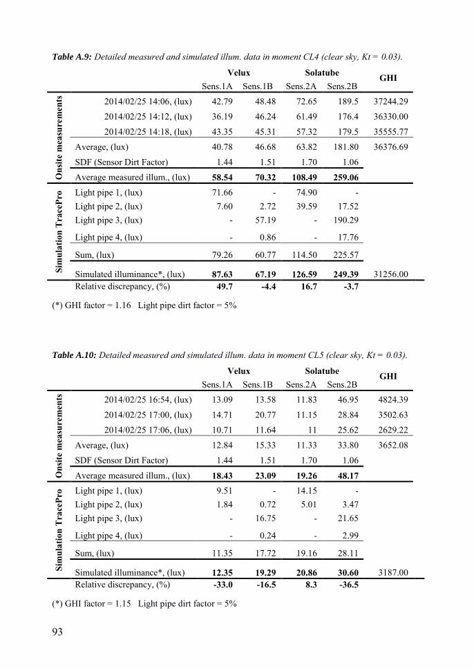
93

Table A.9: Detailed measured and simulated illum. data in moment CL4 (clear sky, Kt = 0.03). Velux Solatube GHI

Sens.1A Sens.1B Sens.2A Sens.2B

Ons

ite m

easu

rem

ents

2014/02/25 14:06, (lux) 42.79 48.48 72.65 189.5 37244.29

2014/02/25 14:12, (lux) 36.19 46.24 61.49 176.4 36330.00

2014/02/25 14:18, (lux) 43.35 45.31 57.32 179.5 35555.77

Average, (lux) 40.78 46.68 63.82 181.80 36376.69

SDF (Sensor Dirt Factor) 1.44 1.51 1.70 1.06

Average measured illum., (lux) 58.54 70.32 108.49 259.06

Sim

ulat

ion

Tra

cePr

o Light pipe 1, (lux) 71.66 - 74.90 - Light pipe 2, (lux) 7.60 2.72 39.59 17.52 Light pipe 3, (lux) - 57.19 - 190.29

Light pipe 4, (lux) - 0.86 - 17.76

Sum, (lux) 79.26 60.77 114.50 225.57

Simulated illuminance*, (lux) 87.63 67.19 126.59 249.39 31256.00 Relative discrepancy, (%) 49.7 -4.4 16.7 -3.7

(*) GHI factor = 1.16 Light pipe dirt factor = 5%

Table A.10: Detailed measured and simulated illum. data in moment CL5 (clear sky, Kt = 0.03). Velux Solatube GHI

Sens.1A Sens.1B Sens.2A Sens.2B

Ons

ite m

easu

rem

ents

2014/02/25 16:54, (lux) 13.09 13.58 11.83 46.95 4824.39

2014/02/25 17:00, (lux) 14.71 20.77 11.15 28.84 3502.63

2014/02/25 17:06, (lux) 10.71 11.64 11 25.62 2629.22

Average, (lux) 12.84 15.33 11.33 33.80 3652.08

SDF (Sensor Dirt Factor) 1.44 1.51 1.70 1.06

Average measured illum., (lux) 18.43 23.09 19.26 48.17

Sim

ulat

ion

Tra

cePr

o Light pipe 1, (lux) 9.51 - 14.15 - Light pipe 2, (lux) 1.84 0.72 5.01 3.47 Light pipe 3, (lux) - 16.75 - 21.65

Light pipe 4, (lux) - 0.24 - 2.99

Sum, (lux) 11.35 17.72 19.16 28.11

Simulated illuminance*, (lux) 12.35 19.29 20.86 30.60 3187.00 Relative discrepancy, (%) -33.0 -16.5 8.3 -36.5

(*) GHI factor = 1.15 Light pipe dirt factor = 5%

94

Table A.11: Detailed measured and simulated illum. data in moment CL6 (clear sky, Kt = 0.01). Velux Solatube GHI

Sens.1A Sens.1B Sens.2A Sens.2B

Ons

ite m

easu

rem

ents

2014/03/12 10:42, (lux) 59.42 55.4 91.5 270.1 49566.00

2014/03/12 10:48, (lux) 52.27 55.27 96.1 274 50760.78

2014/03/12 10:54, (lux) 56.7 63.66 97.3 273.7 51415.62

Average, (lux) 56.13 58.11 94.97 272.60 50580.80

SDF (Sensor Dirt Factor) 1.41 1.65 1.56 1.62

Average measured illum., (lux) 79.10 95.88 148.18 442.07

Sim

ulat

ion

Tra

cePr

o Light pipe 1, (lux) 69.09 - 119.48 - Light pipe 2, (lux) 8.50 1.46 26.31 16.65 Light pipe 3, (lux) - 81.01 - 186.57

Light pipe 4, (lux) - 0.74 - 19.29

Sum, (lux) 77.59 83.21 145.79 222.52

Simulated illuminance*, (lux) 110.07 118.03 206.80 315.64 33875.00 Relative discrepancy, (%) 39.1 23.1 39.6 -28.6

(*) GHI factor = 1.49 Light pipe dirt factor = 5%

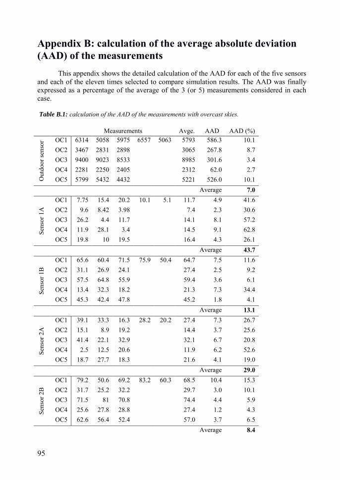
95

Appendix B: calculation of the average absolute deviation (AAD) of the measurements

This appendix shows the detailed calculation of the AAD for each of the five sensors and each of the eleven times selected to compare simulation results. The AAD was finally expressed as a percentage of the average of the 3 (or 5) measurements considered in each case.

Table B.1: calculation of the AAD of the measurements with overcast skies.

Measurements Avge. AAD AAD (%)

Out

door

sens

or OC1 6314 5058 5975 6557 5063 5793 586.3 10.1

OC2 3467 2831 2898 3065 267.8 8.7 OC3 9400 9023 8533 8985 301.6 3.4 OC4 2281 2250 2405 2312 62.0 2.7 OC5 5799 5432 4432 5221 526.0 10.1

Average 7.0

Sens

or 1

A

OC1 7.75 15.4 20.2 10.1 5.1 11.7 4.9 41.6 OC2 9.6 8.42 3.98 7.4 2.3 30.6 OC3 26.2 4.4 11.7 14.1 8.1 57.2 OC4 11.9 28.1 3.4 14.5 9.1 62.8 OC5 19.8 10 19.5 16.4 4.3 26.1

Average 43.7

Sens

or 1

B

OC1 65.6 60.4 71.5 75.9 50.4 64.7 7.5 11.6 OC2 31.1 26.9 24.1 27.4 2.5 9.2 OC3 57.5 64.8 55.9 59.4 3.6 6.1 OC4 13.4 32.3 18.2 21.3 7.3 34.4 OC5 45.3 42.4 47.8 45.2 1.8 4.1

Average 13.1

Sens

or 2

A

OC1 39.1 33.3 16.3 28.2 20.2 27.4 7.3 26.7 OC2 15.1 8.9 19.2 14.4 3.7 25.6 OC3 41.4 22.1 32.9 32.1 6.7 20.8 OC4 2.5 12.5 20.6 11.9 6.2 52.6 OC5 18.7 27.7 18.3 21.6 4.1 19.0

Average 29.0

Sens

or 2

B

OC1 79.2 50.6 69.2 83.2 60.3 68.5 10.4 15.3 OC2 31.7 25.2 32.2 29.7 3.0 10.1 OC3 71.5 81 70.8 74.4 4.4 5.9 OC4 25.6 27.8 28.8 27.4 1.2 4.3 OC5 62.6 56.4 52.4 57.0 3.7 6.5

Average 8.4

96

Table B.2: calculation of the AAD of the measurements with clear skies.

Measurements Avge. AAD AAD (%)

Out

door

sens

or CL1 26712 26998 27016 26908 131.1 0.5

CL2* 18529 17083 15856 17156 915.3 5.3* CL3 34949 34711 32669 34109 960.4 2.8 CL4 37244 36330 35556 36377 578.2 1.6

CL5* 4824 3503 2629 3652 781.3 21.4* CL6 49566 50761 51416 50581 676.7 1.3

Average 1.6

Sens

or 1

A

CL1 34.7 34.9 23.9 31.1 4.9 15.6 CL2* 22.2 24.4 30.2 25.6 3.1 12.0*

CL3 35.3 42.1 38.4 38.6 2.3 6.1 CL4 42.8 36.2 43.4 40.8 3.1 7.5

CL5* 13.1 14.7 10.7 12.8 1.4 11.0* CL6 59.4 52.3 56.7 56.1 2.6 4.6

Average 8.4

Sens

or 1

B

CL1 46.2 53.6 39.9 46.6 4.7 10.0 CL2* 34.9 27.4 34.4 32.2 3.2 10.1*

CL3 52.4 47.5 51.8 50.6 2.1 4.1 CL4 48.5 46.2 45.3 46.7 1.2 2.6

CL5* 13.6 20.8 11.6 15.3 3.6 23.7* CL6 55.4 55.3 63.7 58.1 3.7 6.4

Average 5.8

Sens

or 2

A

CL1 62.9 63.8 51.1 59.3 5.5 9.2 CL2* 46.1 38.2 19.0 34.4 10.3 29.9*

CL3 87.5 87.5 87.5 87.5 0.0 0.0 CL4 72.7 61.5 57.3 63.8 5.9 9.2

CL5* 11.8 11.2 11.0 11.3 0.3 3.0* CL6 91.5 96.1 97.3 95.0 2.3 2.4

Average 7.0

Sens

or 2

B

CL1 160.7 156.7 170.6 162.7 5.3 3.3 CL2* 136.0 124.3 124.8 128.4 5.1 4.0*

CL3 233.8 217.4 204.9 218.7 10.1 4.6 CL4 189.5 176.4 179.5 181.8 5.1 2.8

CL5* 47.0 28.8 25.6 33.8 8.8 25.9* CL6 270.1 274.0 273.7 272.6 1.7 0.6

Average 2.8

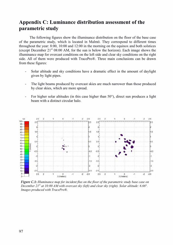
97

Appendix C: Luminance distribution assessment of the parametric study

The following figures show the illuminance distribution on the floor of the base case of the parametric study, which is located in Malmö. They correspond to different times throughout the year: 8:00, 10:00 and 12:00 in the morning on the equinox and both solstices (except December 21st 08:00 AM, for the sun is below the horizon). Each image shows the illuminance map for overcast conditions on the left side and clear sky conditions on the right side. All of them were produced with TracePro®. Three main conclusions can be drawn from these figures:

- Solar altitude and sky conditions have a dramatic effect in the amount of daylight given by light pipes.

- The light beams produced by overcast skies are much narrower than those produced by clear skies, which are more spread.

- For higher solar altitudes (in this case higher than 50°), direct sun produces a light beam with a distinct circular halo.

Figure C.1: Illuminance map for incident flux on the floor of the parametric study base case on December 21st at 10:00 AM with overcast sky (left) and clear sky (right). Solar altitude: 6.66°. Images produced with TracePro®.

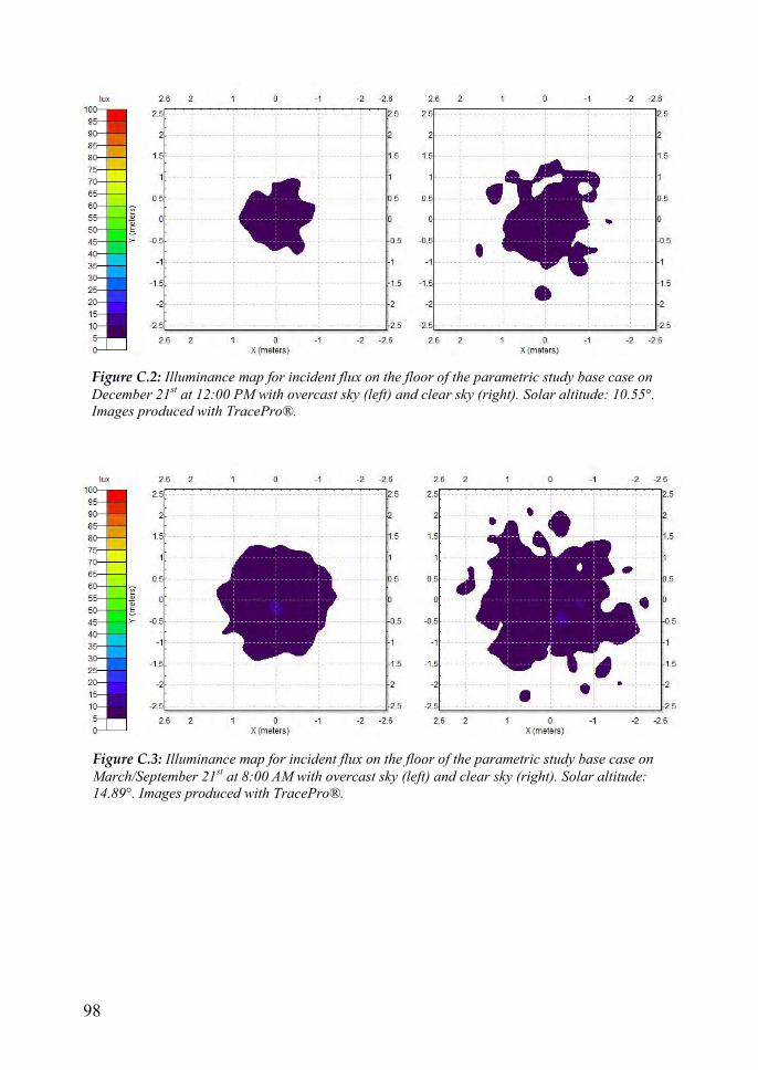
98

Figure C.2: Illuminance map for incident flux on the floor of the parametric study base case on December 21st at 12:00 PM with overcast sky (left) and clear sky (right). Solar altitude: 10.55°. Images produced with TracePro®.

Figure C.3: Illuminance map for incident flux on the floor of the parametric study base case on March/September 21st at 8:00 AM with overcast sky (left) and clear sky (right). Solar altitude: 14.89°. Images produced with TracePro®.

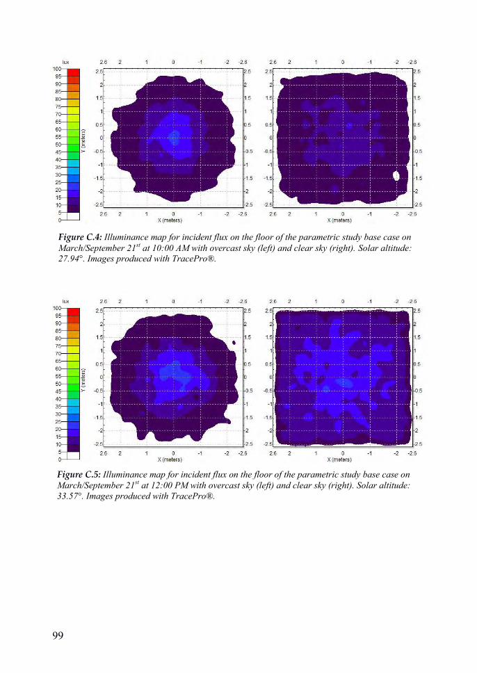
99

Figure C.4: Illuminance map for incident flux on the floor of the parametric study base case on March/September 21st at 10:00 AM with overcast sky (left) and clear sky (right). Solar altitude: 27.94°. Images produced with TracePro®.

Figure C.5: Illuminance map for incident flux on the floor of the parametric study base case on March/September 21st at 12:00 PM with overcast sky (left) and clear sky (right). Solar altitude: 33.57°. Images produced with TracePro®.

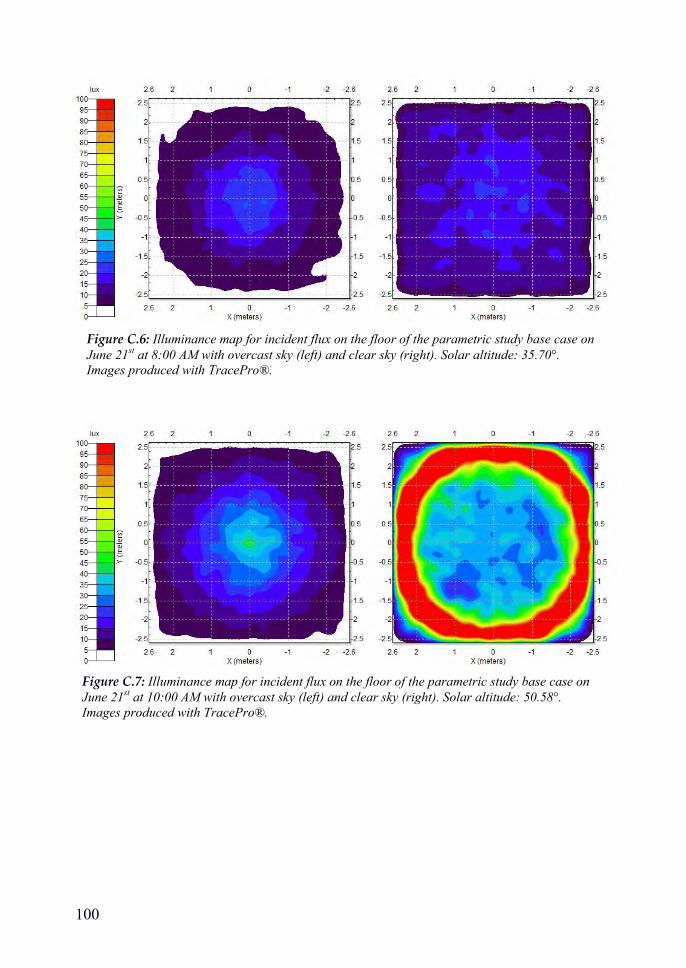
100

Figure C.6: Illuminance map for incident flux on the floor of the parametric study base case on June 21st at 8:00 AM with overcast sky (left) and clear sky (right). Solar altitude: 35.70°. Images produced with TracePro®.

Figure C.7: Illuminance map for incident flux on the floor of the parametric study base case on June 21st at 10:00 AM with overcast sky (left) and clear sky (right). Solar altitude: 50.58°. Images produced with TracePro®.

101

Figure C.8: Illuminance map for incident flux on the floor of the parametric study base case on June 21st at 12:00 PM with overcast sky (left) and clear sky (right). Solar altitude: 57.45°. Images produced with TracePro®.

Dept of Architecture and Built Environment: Division of Energy and Building DesignDept of Building and Environmental Technology: Divisions of Building Physics and Building Services