Changes in Hydrological Conditions and Surface Fluxes

Due to Seasonal Vegetation Greening in the North

American Monsoon Region

by

Luis Arturo Méndez-Barroso

Submitted in Partial Fulfillment of the Requirements for the Degree of Master Degree in

Earth and Environmental Science with Dissertation in Hydrology.

New Mexico Institute of Mining and Technology

Socorro, New Mexico

June 2009

ABSTRACT

The North American monsoon (NAM) region in northwestern Mexico is

characterized by seasonal precipitation pulses which lead to a major shift in vegetation

greening and ecosystem processes. Seasonal greening in the desert region is particularly

important due to its impact on land surface conditions and its potential feedback to

atmospheric and hydrologic processes. In this thesis, we utilize remotely-sensed and

ground-based measurements to infer land surface energy changes that can influence the

NAM through a vegetation-rainfall feedback mechanism. Our study is focused over the

period 2004-2007 for the Río San Miguel and Río Sonora basins, which contain a

regional network of precipitation and soil moisture observations. Results indicate that

seasonal changes in vegetation greenness, albedo and land surface temperature are

dramatic for all regional ecosystems and are related to interannual differences in

hydrologic conditions. Vegetation responses depend strongly on the plant communities in

each ecosystem, with the highest greening occurring in the mid elevation Sinaloan

thornscrub (or subtropical scrubland). Results from the analysis of remote sensing data

indicate that the ground observations at an eddy covariance tower are representative of

the land surface dynamics in subtropical scrublands. This large region exhibits a high

seasonality in vegetation greenness, albedo and land surface temperature. Spatial and

temporal persistence of remotely-sensed Normalized Difference Vegetation Index

(NDVI), albedo and land surface temperature (LST) fields were then used to distinguish

the arrangement of functional groups with cohesive organization by using cluster analysis

and unsupervised classification. We identified six functional groups exhibiting different

surface response in albedo, NDVI and LST. Subtropical scrublands exhibited large

spatial extents in the region with significant seasonal changes in land surface conditions.

The work also indicates that accumulated seasonal precipitation is a strong indicator of

biomass production across the regional ecosystems with higher greenness precipitation

ratio for the Sinaloan thornscrub. Further, precipitation was found to have higher lagged

correlations to the vegetation dynamics, while soil moisture was the primary factor

influencing vegetation greening during concurrent periods. Multiyear comparisons across

ecosystems indicate that different plant water use strategies may exist in response to

interannual hydrologic variations and are strongly controlled by elevation along semiarid

mountain fronts. Finally, analysis of land-atmosphere observations prior to and during the

NAM from an eddy covariance tower are used to infer the necessary conditions for a

vegetation-rainfall feedback mechanism in subtropical scrublands. We find that

precipitation during the monsoon onset leads to changes in vegetation that impact land

surface states and fluxes in such a way as to promote subsequent convective rainfall.

Persistence cloudiness, however, can weaken the feedback mechanism. This land-based

inference of the existence of positive vegetation-rainfall feedback should be corroborated

with atmospheric measurements and modeling.

Keywords: North American monsoon, semiarid ecosystems, ecohydrology, remote sensing, Sonoran Desert, soil moisture, precipitation, vegetation.

ii

ACKNOWLEDGMENTS

This thesis is dedicated to my wife Alma and my daughter Ximena.

Inside us there is something that has no name that something is what we are.

- Jose Saramago

iii

TABLE OF CONTENTS

LIST OF TABLES………………………………………………………………... v

LIST OF FIGURES………………………………………………………………. viii

1 INTRODUCTION…………………………………………………………. 1

1.1 Overview of North American Monsoon Region………………………. 1

1.2 Remote Sensing and Vegetation Monitoring………………………….. 8

1.3 Relation Between Vegetation Indices, Rainfall and Soil Moisture……. 9

1.4 Changes in Surface Conditions and Energy Balance at the Surface…... 11

1.5 Interactions Surface Atmosphere and Possible Feedback Mechanisms.. 12

1.6 Objectives and Goals of this Thesis…………………………………… 15

2 METHODS………………………………………………………………… 16

2.1 Study Region and Ecosystem Distributions………………………….... 16

2.1.1 Sonoran Desert Scrub……………………………………………… 19

2.1.2 Sinaloan Thornscrub………………………………………………. 19

2.1.3 Sonoran Riparian Deciduous Woodland…………………………... 19

2.1.4 Sonoran Savanna Grassland……………………………………….. 20

2.1.5 Madrean Evergreen Woodland…………………………………….. 20

2.1.6 Madrean Montane Conifer Forest…………………………………. 20

2.2 Field and Remote Sensing Datasets…………………………………… 21

2.3 Metrics of Spatial and Temporal Vegetation Dynamics………………. 28

2.3.1 Temporal Variation of Vegetation Metrics……………………… 29

2.3.2 Spatial and Temporal Analysis: The Time Stability Concept……... 35

2.3.3 Elevation Control on Vegetation Statistics……………………… 39

2.4 Relation Between NDVI, Precipitation and Soil Moisture……………. 41

2.5 Cluster Analysis and Unsupervised Classification…………………….. 42

3 RESULTS AND DISCUSSION…………………………………………... 44

3.1 Spatial and Temporal Vegetation Dynamics in Regional Ecosystems 44

iv

3.2 Quantifying Ecosystem Dynamics Through Vegetation………………. 50

3.3 Relations Between Vegetation and Hydrologic Indices……………….. 54

3.4 Spatial and Temporal Stability Analyses of Vegetation Dynamics…… 63

3.4.1 Spatial and Temporal Stability of NDVI…………………………... 63

3.4.2 Spatial and Temporal Stability of Albedo…………………………. 66

3.4.3 Spatial and Temporal Stability of Land Surface Temperature…….. 67

3.5 Topographic Control on Vegetation Dynamics……………………….. 67

3.6 Identifying Land Surface Response Functional Groups………………. 74

3.7 Vegetation-Rainfall Feedback Mechanism in Subtropical Scrubland… 78

4 CONCLUSIONS AND FUTURE WORK………………………………... 83

5 REFERENCES……………………………………………………………. 89

6 APPENDIX 1: Stations datasets………………………………………….. 105

7 APPENDIX 2: Glossary of terms…………………………………………. 135

8 APPENDIX 3: MATLABTM scripts………………………………………... 136

v

LIST OF TABLES

2.1 Regional hydrometeorological station locations, altitudes and ecosystem

classifications. The coordinate system for the locations is UTM 12N, datum

WGS84…………………………………………………………….................... 22

2.2 Missing observations periods at regional stations during 2004 to 2006. Note

that the lower data gaps in the monsoon season of 2005……………………… 23

2.3 Comparison among different lagged time periods and their influence in the

estimation of time integrated EVI (known as iEVI and it is defined as the area

under the curve of vegetation growing season)………………………………... 35

3.1 Comparison of the red and infrared bands for several remote sensing sensors.

Taken from Buheaosier et al., 2003………………………………………………….. 50

3.2 Comparison of vegetation metrics for the regional stations during the three

monsoons……………………………………………………………………… 51

3.3 Coefficient of variation (CV) of vegetation metrics for different ecosystems

during the period 2004-2006. CV is calculated as the temporal standard

deviation divided by the temporal mean averaged over all stations in each

ecosystem (N sites in each ecosystem)………………………………………… 54

3.4 Comparison of iNDVI, precipitation (mm) and greenness-precipitation ratio

(GPR) for the regional station during 2005. Note that data gaps existed for

stations 134 and 140…………………………………………………………… 57

3.5 Linear correlation coefficients between NDVI and accumulated rainfall (mm)

at different monthly lags. Precipitation was accumulated at lag 0: rainfall

vi

accumulated in the current month, 1: rainfall accumulated one month earlier,

2: two months earlier, 3: three months earlier, 0+1: accumulated rainfall in the

current month plus the previous month, 1+2: two previous months, and

0+1+2: current and the two previous months ………………………………….

3.6 Linear correlation coefficients between NDVI and averaged soil moisture at

different monthly lags. Precipitation was accumulated at lag 0: rainfall

accumulated in the current month, 1: rainfall accumulated one month earlier,

2: two months earlier, 3: three months earlier, 0+1: accumulated rainfall in the

current month plus the previous month, 1+2: two previous months, and

0+1+2: current plus two previous months……………………………………... 61

3.7 Error matrix showing the comparison between the new functional groups map

and a reference map (Land cover map generated by Yilmaz et al., 2008). The

classes shown horizontally represent the classes of the reference map;

conversely, the classes shown vertically represent the classes in the generated

map. The number of pixels shaded and shown diagonally represents the

number of correctly classified pixels by category……………………………... 76

3.8 Functional group characteristics, including the direction of change in the

spatially-average land surface property (NDVI, albedo, LST) during the

monsoon transition: increase (+), decrease (-) and no net change (±). See

Figure xx for the spatial variability. Number of pixels refers to the MODIS

pixel resolution (~1 km2) in parenthesis is the percent of the total area………. 78

3.9 Comparison of changes in ground-based and remotely sensed variables at the

Rayón EC tower. Before monsoon has 34 days: DOY 151 (May 31, 2007) to

59

vii

DOY 184 (July 3, 2007). During monsoon period has 56 days DOY 185 (July

3, 2007) to DOY 240 (August 28, 2007)……………………………………….

3.10 Comparison of changes in ground observations during two-days sequences

exhibiting a positive vegetation-rainfall feedback (Day 1 and 2 = Julian day

201 and 202) and a weakened feedback due to the effects of cloudiness (Day

1 and 2 = Julian days 215 and 216)……………………………………………. 82

81

viii

LIST OF FIGURES

1.1 Vegetation greening in the study region during (a) June 30, 2007 and (b)

August 12, 2008. Note the mountainous terrain (~820 m) and the Sinaloan

thornscrub ecosystem………………………………………………………...... 2

2.1 Location of the Río San Miguel and Río Sonora basins in Sonora, Mexico

including hydrologic stations and an eddy covariance tower. Topographic

features are shown by means of a hillshaded 29-m Digital Elevation Model.

Land cover classes correspond to the National Institute of Statistics,

Geography and Informatics of Mexico (INEGI, 2008)………………………... 17

2.2 Regional cross-section with the distribution of the ecosystems. Elevation is

expressed as meters above sea level…………………………………………… 21

2.3 Diagram of MODIS compositing method. Taken from Huete et al., 2002……… 26

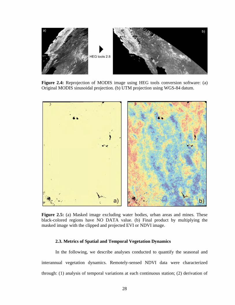
2.4 Reprojection of MODIS image using HEG tools conversion software: a)

Original MODIS sinusoidal projection. b) UTM projection conversion using

WGS-84 datum………………………………………………………………… 28

2.5 a) Masked image excluding water bodies, urban areas and mines. These

black-colored regions have NO DATA value. b) Final product by multiplying

the masked image with the clipped and projected EVI or NDVI image………. 28

2.6 Extraction of pixel values. The red dot represents the station location and the

pixel beneath the location is considered the central pixel. Then for the

estimation of the mean value, we took into consideration the eight values

around the central pixel. ……………………………………………………… 30

ix

2.7 Determination of vegetation metrics. (a) Identification of the beginning and

end of the vegetation greening using the smoothed NDVI series and the

backward (BMA) and forward (FMA) moving averages for station 130

(Sinaloan thornscrub). The original NDVI data is represented by the open

circles. (b) Example of the vegetation metrics (iNDVI, NDVI, Rate of

Greenup, Rate of Senescence and Duration of Greenness) for station 130

during the 2004 season………………………………………………................

2.8 Sensitivity analysis for Forward Moving Average (FMA). The number of

lagged time periods was changed to 2, 3, 4, 5, 6 and 7 in order to get the point

where vegetation greenness starts……………………………………………... 34

2.9 Sensitivity analysis for Backward Moving Average (BMA). The number of

lagged time periods was changed to 2, 3, 4, 5, 6 and 7 in order to get the point

where vegetation greenness ends……………………………………………… 34

2.10 Temporal evolution of mean spatial NDVI and surface albedo during the

study period. Every point in the plot represents a mean spatial value used to

estimate the spatial RMSE of the difference…………………………………... 36

2.11 Temporal mean NDVI, surface albedo and land surface temperature used to

estimate the temporal RMSE of the difference. Every images is the result of

averaging 83 MODIS composite images……………………………………… 36

2.12 Location of the two topographic transects for Rio Sonora and Rio San Miguel

Basin. Each transect is ~23 km in length, samples elevations from nearly 600

m to 1600 m above sea level, and traverses different ecosystems along the

elevation gradient…………………………………............................................ 40

32

x

3.1 Comparison of seasonal NDVI change (%). The percentage of NDVI change

is calculated using the lowest and highest NDVI for a particular summer

season (2004 to 2006). sR is the total summer rainfall (July to September)

averaged over all regional stations……………………………………………..

3.2 Temporal variation of NDVI among different regional ecosystems: (a)

Madrean evergreen woodland (station 146), (b) Sinaloan thornscrub (station

132), (c) Sonoran savanna grassland (station 139), and (d) Sonoran desert

scrub (station 144). NDVI symbols correspond to the average value

calculated in the 3 3 pixel region around each station for each composite.

The vertical bars depict the ±1 standard deviation of the 3 3 pixel region.

Precipitation (mm) is accumulated during 16-day intervals and shown as gray

bars, while the averaged surface volumetric soil moisture (%) during the 16-

day periods is shown as open circles………………………………................... 47

3.3 Relation between the seasonal precipitation accumulation and iNDVI for the

monsoon season in 2005. Each point is a station located in a different

ecosystem……………………………………………………………………… 58

3.4 Linear correlation coefficients (CCs) between monthly NDVI and

accumulated precipitation and averaged soil moisture over a range of different

monthly lags, arranged from current (lag 0) toward longer prior periods (lag

0+1+2). CCs are shown as averages (symbols) and standard deviations (±1 std

as vertical bars) over all stations in 2005……………………………………… 61

45

xi

3.5 Comparison between surface soil moisture and root zone profile at station 147

(Rayon tower). Dots represents mean daily values and the bars ±1 standard

deviation………………………………………………………………………. 62

3.6 Spatial distributions of spatial and temporal RMSE for: (a, b) NDVI, (c, d)

Albedo and (e, f) LST. The pixel resolution for NDVI is 250-m, whereas

albedo and LST are 1-km……………………………………………………… 64

3.7 Topographic control on vegetation metrics in the Río San Miguel transect. (a)

Relation between elevation and temporal mean NDVI (closed circles) and the

temporal standard deviation (±1 std as vertical bars). (b) Relation between

elevation and spatial and temporal RMSE ...................................................... 69

3.8 Topographic control on vegetation metrics in the Río Sonora transect. (a)

Relation between elevation and temporal mean NDVI (closed circles) and the

temporal standard deviation (±1 std as vertical bars). (b) Relation between

elevation and spatial and temporal RMSE …………………………………... 70

3.9 Topographic control on albedo in the Río San Miguel. (a) Relation between

elevation and temporal mean albedo (closed circles) and the temporal

standard deviation (±1 std as vertical bars). (b) Relation between elevation

and spatial and temporal RMSE ……………………………………………... 72

3.10 Topographic control on land surface temperature in the Río San Miguel. (a)

Relation between elevation and temporal mean albedo (closed circles) and the

temporal standard deviation (±1 std as vertical bars). (b) Relation between

elevation and spatial and temporal RMSE …………………………………... 73

xii

3.11 (a) Land surface response functional groups obtained from cluster analysis.

Mean spatial percent change during NAM for each functional group for: (b)

NDVI, (d) Albedo and (f) LST. Error bars represent ± 1 spatial standard

deviation. Relation between mean spatial and temporal RMSE by functional

group for: (c) NDVI, (e) Albedo and (g) LST. Functional groups are ordered

with increasing elevation (see legend for functional group name)……………. 77

3.12 (a) Transition in NDVI, albedo, Bowen ratio and precipitation during the

2007 monsoon season. (b) Transition of soil temperature, net radiation, soil

moisture and precipitation. Gaps in net radiation correspond to cloudy days

not included in analysis. (c) Diagram relating changes in soil moisture and

vegetation greenness with the subsequent effects in land-atmosphere

interactions and rainfall, adapted from Eltahir (1998)………............................

80

This dissertation is accepted on behalf of the faculty of the Institute by the

following committee:

Dr. Enrique R. Vivoni

________________________________________________________________________

________________________________________________________________________

________________________________________________________________________

________________________________________________________________________

________________________________________________________________________

________________________________________________________________________

Date

1

CHAPTER 1

INTRODUCTION

This section describes the North American Monsoon and its main characteristics.

In addition, we briefly discus the relation between vegetation greening, precipitation and

soil moisture as well as the remote sensing approach to monitoring vegetation dynamics.

This shift in vegetation dynamics lead to large changes in surface conditions (energy

balance and depth of boundary layer), which can promote subsequent convective rainfall,

hence, a hypothesized positive vegetation-rainfall feedback mechanism.

1.1. Overview of North American Monsoon Region

The North American Monsoon (NAM) is an important meteorological

phenomenon causing an increment in rainfall in northwestern Mexico and southwestern

United States. The core of monsoon precipitation, in the months of July, August and

September, is located in the western slope of Sierra Madre Occidental (Gochis et al.,

2004). Precipitation in areas peripheral to this core region shows high spatiotemporal

variability due to transient features such as the passage of tropical easterly waves (Fuller

and Stensrud, 2000). The region is generally semiarid with an annual precipitation regime

dominated by warm season convection that strongly interacts with the regional

topography. Conditions before monsoon onset are characterized by high temperatures and

2

Figure 1.1: Vegetation greening in the study region during (a) June 30, 2007 and (b) August 12, 2008. Note the mountainous terrain (~820 m) and the Sinaloan thornscrub ecosystem.

minimal rainfall. The monsoon transition is well documented in several articles (Douglas

et al., 1993; Higgins et al., 1997; Higgins and Shi, 2000), among others. There is a

seasonal surface wind reversal over some areas affected by the North American

monsoon, notably the Gulf of California (Badan-Dangon et al. 1991), a reversal that is

similar to but a much smaller scale to the Asian Monsoon. Krishnamurti (1971) noted

that there were two planetary scale east-west (or monsoonal) circulations, a dominant one

associated with Asia and a much weaker one associated with the Mexican plateau in the

summer. Histograms of monthly mean rainfall and mean temperature for many of the

stations in northwest Mexico are similar to those in southern Asia with most of the annual

rainfall taking place during a short period (2-4 months) and with the highest temperature

3

just prior to the onset of rains (Douglas et al. 1993). The geographical extent of the NAM

includes the region surrounding the southern part of the Gulf of California, the axis of the

Sierra Madre Occidental extending into southeastern Arizona, the Rio Grande Valley in

New Mexico and into the high plains of southern Colorado. However, the NAM is most

spatially consistent over northwest Mexico with greater variability to the north.

As an ocean–atmosphere-land coupled system, the NAM exhibits apparent

dependence on land and ocean surface conditions (Adams and Comrie 1997). For this

reason, pre-monsoon land surface and oceanic conditions are promising predictors for

NAM precipitation at seasonal lead times, especially where these predictors are

temporally persistent. Higgins et al. (1999) examined the relation between anomalous

monsoon behavior over Arizona-New Mexico, NW Mexico and SW Mexico, and the El

Niño Southern Oscillation (ENSO) signals. They found that wet (dry) conditions in

southwest Mexico tend to occur during La Niña (El Niño), which they attribute partly to

the impact of local sea surface temperature (SST) on the land sea thermal contrast, hence

the strength of the monsoon. They also found a weak association between dry monsoons

in NW Mexico and El Niño. Hu and Song (2002) showed that south central Mexico

monsoon rainfall is highly affected by interannual variations in SST and the location of

the intertropical convergence zone (ITCZ) in the eastern tropical pacific. Cooler (warmer)

than normal SST co-existed with the more northern (southern) position of ITCZ and more

(less) monsoon rainfall in central-south Mexico.

Matsui et al. (2003) investigated the influence of land-atmosphere interactions on

the variability of the NAM by testing a hypothesis regarding the connection between

observed land surface variables (April snow water equivalent, surface temperature and

4

precipitation) in the NAM region, including NW Mexico, for the period 1979-2000. Their

result showed that there is a weak negative relationship between April snow water

equivalent in the Rocky Mountain region and subsequent spring temperatures that persist

into June in the NAM region. They concluded that this inverse relationship could not

directly influence monsoon rainfall in July and August because it disappears during the

monsoon season. These results are similar to those found by Small (2001) who showed

an inverse relation between southern Rocky Mountains antecedent season snowpack and

monsoon rainfall. Zhu et al. (2007) found that soil moisture anomalies correlate

negatively with surface temperature anomalies over most of the U.S. and Mexico, except

in the desert regions. The onset of the monsoon is negatively correlated to May surface

temperature, suggesting that antecedent land surface conditions may influence the pre-

monsoon thermal conditions, which then affects monsoon onset. They also confirmed

that the strength of the monsoon is related to pre-monsoon land-sea surface temperature

contrast. This statement confirms that late monsoon years are associated with colder land

and warmer adjacent ocean than early monsoon years. In addition, a strong positive

relation between May surface temperature anomalies and the large-scale mid-

tropospheric circulation anomalies was found which suggest that large-scale circulation

may play a strong role in modulating the monsoon onset. In fact, the role of the large-

scale circulation may well be larger than the apparent land surface feedback effect.

The role of vegetation after precipitation onset and the subsequence changes in

land surface processes are poorly understood in the context of the land surface effects on

the monsoon. A few studies have started to address the seasonal changes in vegetation

greenness, surface fluxes, and soil moisture (Watts et al., 2007; Vivoni et al., 2008b). The

5

NAM is the main climate phenomenon controlling summer rainfall in northwestern

Mexico and the southwestern U.S. (Douglas et al., 1993; Adams and Comrie, 1997;

Sheppard et al., 2002) and accounts for ~40 to 70% of the annual precipitation in the

region. Understanding vegetation dynamics and its relation to hydrologic conditions

during the NAM is important as this period coincides with the plant greening and

growing season in the region (Watts et al., 2007). Fig. 1.1 is an example of the vegetation

greening observed in the mountainous study area of northwestern Mexico.

The ecohydrology of northwestern Mexico is particularly interesting as the

seasonal precipitation pulses from the NAM lead to a major shift in vegetation greening

and ecosystem processes. Plant responses during the monsoon include the production of

leaf biomass required for photosynthesis, flowering and seed dispersal (e.g., Reynolds et

al., 2004; Weiss et al., 2004; Caso et al., 2007). The vegetation transition occurs

relatively rapidly and is closely tied to the monsoon onset and its variability.

Few studies exist to understand the relation between climatic variables and

vegetation greening in Mexico. Gomez-Mendoza et al. (2008) found that NDVI values

for several vegetation types are correlated with the spatial and temporal variability of

precipitation in the Mexican state of Oaxaca. Nevertheless, they observed intraannual

changes in the response time of vegetation to the onset and distribution of precipitation.

Their results suggest that temperate forest may be considered as good indicators of inter-

annual climate variability, whereas, tropical dry forest and grasslands are more sensitive

to intraannual variability. Precipitation pulses are essential for the regeneration of

drylands in northwest Mexico. Caso et al. (2007) found that El Niño events tend to

increase rainfall in northwest Mexico, but tend to increase aridity in the southern tropical

6

Pacific slope. El Niño produced a large increase in winter rainfall above 22 degrees

latitude, whereas La Niña conditions tend to produce an increase in summer monsoon

type rainfall that predominates in the tropical south. In addition, Salinas-Zavala et al.

(2002), found that the negative ENSO phase is associated with drought conditions with

delay of 4-6 months related to the start of the event, while the positive phase is related to

high NDVI values during the driest season in the region. Summers with high NDVI

values are related to an intensification of the summer monsoon, while, in dry summers,

the regional atmospheric circulation is characterized by the presence of an enhanced ridge

of high pressure aloft over most of Mexico. Mora et al. (1998) found significant non-

linear relations between vegetation productivity, precipitation and evapotranspiration in

Mexico. Variation of vegetation pattern of productivity and seasonality is explained less

at the ecoregion scale relative to the country level, but water balance variables still

account for more than 50% of the variation in vegetation.

The climate conditions in Mexico lead to a gradual replacement of the Sonoran

Desert by the subtropical thornscrubs and dry forest of Sinaloa (Caso et al, 2007). Farther

into the tropics, a long corridor of tropical dry deciduous forest runs along the coast in

Jalisco and Chiapas (Martin et al., 1998). The Sonoran Desert receives winter

precipitation in its northwestern reaches near the Mojave Desert, but is fed predominantly

by summer monsoon rains in its tropical southern boundary with the Sinaloan thornscrubs

(Dimmit et al., 2000). Tropical summer-rain drylands in western and southern Mexico are

dominated by drought deciduous trees and shrubs, often with succulent stems or fleshy

trunks and tropical evolutionary origins (Bullock et al., 1995). Despite its high

biodiversity and biomass production, this ecosystem is one of the most threatened

7

vegetation types in Mexico. In Sonora, this biome has been replaced by introduced

species as buffel grass as result of land use changes (Arriaga et al., 2004). The three main

pathways of vegetation changes associated with land use changes in tropical deciduous

forest in Mexico have been documented as: (1) Forest replaced by agriculture in flatlands,

(2) pasture established on slopes and (3) wood extraction carried out without slash and

burn on hillcrests. If cultivated areas in flatlands and pasture fields on slopes are not

continuously maintained by farmers, thorny vegetation can develop within one to 3 years.

If left untouched, this secondary vegetation becomes a low forest dominated by thorny

species (Burgos and Maass, 2004, Alvarez-Yépiz et al., 2008). Losses in total above

ground biomass can account up to 80% as result of slash fires in tropical deciduous

forest, where the dramatic loss of biomass may affect future site productivity and the

capacity for these sites to function as carbon pools (Kauffman et al., 2003).

While the seasonally dynamics of the subtropical and tropical ecosystems in

northwest Mexico has been recognized previously (e.g., Brown, 1994; Salinas-Zavala et

al., 2002), the linkage between hydrologic conditions and ecosystem responses has not

been quantified primarily due to a lack of observations in the region. Fortunately, the

scarcity of field observations has been recently addressed through the North American

Monsoon Experiment (NAME) and Soil Moisture Experiment 2004 (SMEX04) (Higgins

and Gochis, 2007; Watts et al., 2007; Vivoni et al., 2007, 2008a; Bindlish et al., 2008).

As a result, an opportunity exists to quantify vegetation dynamics from remote sensing

data and relate these directly to ground-based observations. For example, Vivoni et al.

(2008a) analyzed soil moisture for different ecosystems arranged across an elevation

gradient through field and remote sensing observations

8

1.2. Remote Sensing and Vegetation Monitoring

Remote sensing from satellite platforms has become an indispensable tool for

monitoring the phenological status of vegetation and its potential role in controlling the

land surface energy and water balance in terrestrial ecosystems (e.g., Xinmei et al., 1993;

Guillevic et al., 2002; Bounoua et al., 2000; Wang et al., 2006; Watts et al., 2007;

Méndez-Barroso et al., 2008). The spatiotemporal characteristics of remote sensing data

provide an advantage as compared to ground observations by allowing quantification of

vegetation phenological changes over large areas and extended periods. For example, the

Normalized Difference Vegetation Index (NDVI) is a useful ratio widely used to estimate

seasonal changes in plant greenness (Sellers, 1985; Tucker et al., 1985; Goward, 1989;

Anyamba and Estman, 1996; Zhang et al., 2003). NDVI is based on the reflectance

properties of green vegetation and is determined by the ratio of the amount of absorption

by chlorophyll in the red wavelength (600-700 nm) to the reflectance of the near infrared

(720-1300 nm) radiation by plant canopies. Through the use of spatiotemporal NDVI

fields, the seasonal and interannual changes in vegetation greenness can be analyzed and

related to biotic and abiotic factors, including rainfall, fire and land cover disturbances

(Zhang et al., 2004; Franklin et al., 2006; Wittenberg et al., 2007).

Currently, one of the most reliable sources of remotely-sensed NDVI data is the

MODIS (Moderate Resolution Imaging Spectroradiometer) sensor on board the EOS

Terra and Aqua satellites (Huete et al., 1997, 2002). This sensor offers excellent

radiometric and geometric properties, as well as improved atmospheric and cloud

corrections (see Huete and Liu, 1994 for details). For studies of vegetation phenology,

MODIS products can be used to indicate the spatial and temporal variations in: (1) the

9

onset of photosynthesis, (2) the peak photosynthetic activity, and (3) the senescence,

mortality or removal of vegetation (e.g., Reed et al., 1994; Zhang et al., 2003).

In recent work, Lizarraga-Celaya et al. (2009) found a gradient in MODIS-based

vegetation indices and albedo as a function of latitude in the NAM region. A large inter-

seasonal variability can be observed in the tropical deciduous forests (in the southern

state of Jalisco and Durango), while there is a small variability in the grasslands located

in Arizona. In addition, the authors found different responses in the inter-seasonal albedo

at northern latitudes in the NAM region (grasslands and open shrublands) as compared to

the southern region. In this thesis, we use MODIS-derived NDVI fields to examine a set

of semiarid, mountainous ecosystems in northwestern Mexico, which respond vigorously

to summer precipitation during the North American monsoon (Salinas-Zavala et al.,

2002; Watts et al., 2007; Vivoni et al., 2007)

1.3. Relation between Vegetation Indices, Rainfall and Soil Moisture

Seasonal characteristics of vegetation dynamics, such leaf emergence or

senescence, are strongly linked with atmospheric conditions and surface processes such

as rainfall, soil moisture and temperature. As a result, the detection of phenological

changes in entire ecosystems from remote sensing may allow us to monitor seasonal

variability as well as distinguish spatial patterns in hydrologic processes. In prior studies,

remote sensing of vegetation has yielded metrics that are useful for monitoring ecosystem

changes (e.g., Lloyd et al., 1990; Reed et al., 1994; Zhang et al., 2003). An important

contribution has been the time integrated NDVI (iNDVI) over a seasonal period, which is

related to the net primary productivity (NPP) in an ecosystem (Reed et al., 1994). iNDVI

10

measures the magnitude of greenness integrated over time and reflects the capacity of an

ecosystem to support photosynthesis and produce biomass. The relation between rainfall

and iNDVI has been utilized as an indicator of ecosystem productivity. For example,

Prasad et al. (2005) and Li et al. (2004) used iNDVI to study the relation between

precipitation and vegetation in several ecosystems in India and Senegal, respectively. In

both studies, iNDVI showed a strong relationship with rainfall, suggesting this method

may be useful for inferring hydrologic controls on vegetation dynamics in other regions.

Relations between vegetation and precipitation have been studied widely in water-

limited ecosystems. In previous studies, the maximum photosynthetic activity in the plant

growing season has been linked with precipitation in the current and preceding months

(Davenport and Nicholson, 1993; Wang et al., 2003; Al-Bakri and Suleiman, 2004;

Chamaille-Jammes et al., 2006; Prasad et al., 2007). For water-limited ecosystems, the

greenness-precipitation ratio (GPR) has been used to infer the productivity of different

plant associations (Davenport and Nicholson, 1993; Prasad et al., 2005). GPR is defined

as the net primary productivity per unit of rainfall (Le Houerou, 1984). Although

vegetation growth is correlated to rainfall, the incoming precipitation is also modified by

the soil water balance, such that soil moisture is a key intermediary between storm pulses

and plant available water (Breshears and Barnes, 1999; Loik et al., 2004). For example,

Farrar et al. (1994) found that the correlation between NDVI and soil moisture is a

concurrent effect, suggesting a direct linkage between vegetation dynamics and soil

wetness. In addition, the authors found that the accumulated precipitation over several

prior months was related to the vegetation response. Grist et al. (1997) also found

discrepancies in NDVI-rainfall relations and attributed these to soil moisture.

11

1.4. Changes in Surface Conditions and Energy Balance at the Surface

It has well known that land surface and atmospheric processes are interrelated

(e.g., Pielke et al., 1998). For example, changes in soil moisture alter the surface albedo

and the partitioning of turbulent fluxes, with potential effects on convective rainfall

(Eltahir, 1998). The explicit link between vegetation changes and their subsequent effects

on rainfall have been less explored, though Brunsell (2006) indicates these are more

relevant than soil moisture variations. In the NAM region, remote sensing datasets allow

for monitoring of land surface conditions that can be useful for inferring changes that

may promote (positive feedback) or suppress (negative feedback) subsequent rainfall.

Brunsell (2006) found through remotely-sensed LST and NDVI that the NAM region

exhibited a positive land surface-precipitation feedback. Nevertheless, the feedback was

found through correlations with precipitation that do not necessarily indicate causality.

In this thesis, remotely-sensed and ground-based observations are used to infer the

existence of a vegetation-rainfall feedback in the NAM region by tracking the necessary

land surface conditions. Identifying a feedback mechanism in this manner involves

inspection of three variables from remote sensing: NDVI, LST and albedo. NDVI is

related to chlorophyll amount and energy absorption and is indicative of vegetation

phenology (Tucker, 1979). LST is indicative of soil moisture availability and

evapotranspiration and thus closely linked with vegetation function (Matsui et al., 2003;

Brunsell, 2006). Surface albedo is also regulated by soil moisture and vegetation

conditions and has important controls on the radiation budget. After the monsoon onset,

the seasonal vegetation greening should alter the land surface temperature, albedo and

12

surface turbulent fluxes (e.g., evapotranspiration) and lead to changes in boundary layer

conditions that promote more convective rainfall.

The remote sensing and ground-based data are used together in the following

manner. With the satellite data, zones (or functional groups) with similar responses in

terms of NDVI, albedo and LST are identified, since these are strongly related to the

water and energy balances. This permits an assessment of the representativeness of an

eddy covariance tower in the region. Remote sensing data are then compared with ground

measurements at the tower to ensure consistency. Finally, changes in land surface

conditions (e.g., surface fluxes, soil moisture and temperature) are used to infer the

existence and sign of the vegetation-rainfall feedback.

1.5. Interactions Surface-Atmosphere and Possible Feedback Mechanisms

The total energy in the atmospheric boundary layer can be described by moist

static energy (mse), which includes potential energy, sensible heat and latent heat

(Eltahir, 1998):

LqTCgzmse p ++= , (1.1)

where g is the acceleration of the gravity, z is the elevation, Cp is the specific heat

capacity at constant pressure, T is temperature, L is latent heat of vaporization and q is the

water mixing ratio. Moist static energy is supplied by the total heat flux from the surface

into the atmosphere (F). This energy reservoir is depleted by a combination of three main

processes: (1) Entrainment at the top of the boundary layer (EN), (2) Radiative cooling

flux (R), and (3) the negative heat fluxes associated with convective downdraft during

rainfall events (C). If we consider large spatial scales, we can neglect horizontal heat

13

fluxes and only consider vertical heat fluxes from the surface, then the moist energy

budget is transformed to:

CRENFt

mse= . (1.2)

The total heat flux from the surface into the atmosphere is the main source of energy into

the atmospheric boundary layer. Wet soil conditions should favor a larger magnitude of

moist static energy in the atmospheric boundary layer due to a decrease in sensible heat

flux and the rate of entrainment. These factors tend to increase the magnitude of moist

static energy per unit mass of boundary layer air and reduce the boundary layer depth.

Boundary layer moist static energy plays an important role in the dynamics of

local convective storms. At local scales, Williams and Reno (1993) found that wet bulb

potential temperature (a measure of boundary layer moist static energy) is correlated with

convective available potential energy (CAPE). CAPE is an important variable that

describes the atmospheric environment of local convective storms. When CAPE is large,

the atmosphere will be more unstable. However, convection also depends on the

convective inhibition (CIN) that is the amount of energy needed to elevate an air parcel

up to the level of free convection. Large values of CIN imply large resistance to

convective development. Therefore, favorable conditions for convection and precipitation

are identified by large values of CAPE and small values of CIN. For example, reduced

soil moisture in the surface with a drier and warmer boundary layer, reduces the CAPE

with a systematic decreases of about 30% throughout the month (Collini et al., 2008).

Eltahir and Pal (1996) studied the relation between surface wet bulb temperature

and subsequent rainfall in convective storms using observation in the Amazon. They

found that the frequency and the magnitude of localize convective storms increases with

14

surface bulb temperature which confirms that the boundary layer moist static energy

plays an important role in the dynamics of the convective storms. Adams et al. (2009)

found that the North American monsoon convective regime requires essentially only

moisture advection interacting with the strong surface sensible heating over complex

topography. Elimination of strong convective inhibition through intense surface sensible

heating in the presence of sufficient water vapor leads to the positive CAPE-precipitation

relationship on diurnal time scales. In fact, the results from Adam et al. (2009) contradict

results from other continental and maritime regions, which show negative correlations.

In general, recycling refers to how much of the evapotranspiration (ET) in an area

contributes to the precipitation in the same area. As the area is reduced to a point, the ET

contribution tends to zero and all the moisture precipitated is transported in from outside

the region. Eltahir and Bras (1996) reviews estimates of precipitation recycling and

Eltahir and Bras (1994) estimates that 25- 35% of the rain that falls in the Amazon is

contributed by evaporation within the basin. In the Mississippi Basin the recycling

estimates range between 10-24%. Dominguez et al. (2008) shows that evapotranspiration

is responsible for a positive feedback in the NAM onset. Recycling ratios during the

NAM are consistently above 15% and can be as high as 25%. Furthermore, they found

that long monsoons present a characteristic double peak in precipitation where intense

precipitation during July is followed by a period of dry conditions, and then followed by

subsequent peak in late August. The author also established a feedback mechanism for

long monsoons where evapotranspiration is originated predominantly in tropical dry

forests then transported north and east where it later falls as precipitation.

15

1.6. Objectives and Goals of this Thesis

Among the main objectives in this thesis include:

1. To use of remote sensing to quantify the seasonal and interannual

vegetation dynamics in the NAM region and relate these to ground-based

measurements of precipitation and soil moisture.

2. To identify possible relations between vegetation indices, precipitation

and soil moisture as tool for prediction in the region. In addition, it is

important to identify the ecosystems, which are more efficient in

producing vegetation biomass with a smaller precipitation amount.

3. To evaluate the temporal and spatial persistence of land surface conditions

in order to identify regions that are highly seasonally variable, as well as

ecosystems that represent well the spatial mean of the domain.

4. To evaluate the changes in land surface conditions (e.g., surface fluxes,

soil moisture and temperature) to infer the existence and sign of the

vegetation-rainfall feedback.

Few studies have been conducted in the NAM region to understand the role of

vegetation during the monsoon season. This work is important because relatively little

knowledge exists on the interaction between the North American monsoon and land

features such as vegetation dynamics. In addition, vegetation dynamics have received less

attention among the factors that can influence the North American Monsoon.

16

CHAPTER 2

METHODS

In the following, we describe the study region in northwest Mexico, the

continuous precipitation and soil moisture observations, and the remotely-sensed datasets

processed from the MODIS sensor. We selected a three year period (2004 to 2006, with

portions of 2007) to capture vegetation dynamics and change in land surface conditions

during three separate monsoon seasons that exhibited different rainfall amounts and

coincided with the operation of the regional network. We also describe a set of

spatiotemporal analyses used to investigate the relationships between precipitation, soil

moisture and vegetation dynamics, as well as, land surface conditions for different

ecosystems in the mountainous region.

2.1. Study Region and Ecosystem Distributions

Our study region is a large domain that encompasses the Río San Miguel and Río

Sonora basins in northwest Mexico in the state of Sonora (Fig. 2.1). The total area for

both watersheds is ~15,842 km2 (3798 km2 for the Río San Miguel and 11,684 km2 for

the Río Sonora). Our analysis extends beyond the basin boundaries to cover an area of

53,269 km2 including portions of the Río Yaqui and San Pedro River basins. The study

region is characterized by complex terrain in the Sierra Madre Occidental with north-

south trending mountain ranges. The two major ephemeral rivers are Río San Miguel and

Río Sonora, which run from north to south. Basin areas were delineated from a 29-m

digital elevation model (DEM) using two stream gauging sites as outlet points (Fig. 2.1).

17

Figure 2.1: Location of the Río San Miguel and Río Sonora basins in Sonora, Mexico including hydrologic stations and an eddy covariance tower. Topographic features are shown by means of a hillshaded 29-m Digital Elevation Model. Land cover classes correspond to the National Institute of Statistics, Geography and Informatics of Mexico (INEGI, 2008).

For the Río San Miguel, the outlet is a gauging site managed by the Comisión

Nacional del Agua (CNA) known as El Cajón (110.73° W; 29.47° N), while the Río

Sonora was delineated with respect to the El Oregano CNA gauge (110.70° W; 29.22°

N). Elevation above sea level in the region fluctuates between 130 and 3000 m, with a

mean elevation of 983 m and a standard deviation of 391 m. The mean annual

precipitation in the region varies approximately from 300 to 500 mm and it is controlled

by latitudinal position and elevation (Chen et al., 2002; Gochis et al., 2007). A wide

18

variety of ecosystems are found in the study region due to the strong variations in

elevation and climate in short distances (e.g., Brown, 1994; Salinas-Zavala et al., 2002;

Coblentz and Riitters, 2004). Ecosystems are arranged along elevation gradients in the

following fashion (from low to high elevation): Sonoran desert scrub, Sinaloan

thornscrub, Sonoran riparian deciduous woodland, Sonoran savanna grassland, Madrean

evergreen woodland and Madrean montane conifer forest.

Brown (1994) presented the following ecosystem descriptions. Vegetation type in

Sonora is strongly related to elevation. Lowlands are found in the coastal plains adjacent

to the Gulf of California and are characterized by trees less than 3 meters in height and a

small number of thorny tropical species (Figure 2.2). Foothills of Sonora are

characterized by the location of tropical deciduous forest which contains a high diversity

in tropical tree species (30 to 49 species per acre). Usually, tropical forests are followed

by oak woodlands. In the region, they are found in two ways: (1) as a narrow band

between tropical forest and pine forest (about 1000 m) and a savanna-like woodland that

is common in the east slope of the Sierra Madre Occidental. Oak-dominated vegetation

also occurs on smaller scales at lower elevations in narrow canyons and altered acid soils.

Finally, pine-oak forest is the most extensive vegetation type in the high elevations of the

northern Sierra Madre Occidental (about 1300 to 1800 m). At least two dozens of species

of oaks and 13 pines are found in the region (Martin et al., 1998). In the following

sections, we will describe in more details the characteristics of the principal ecosystems.

19

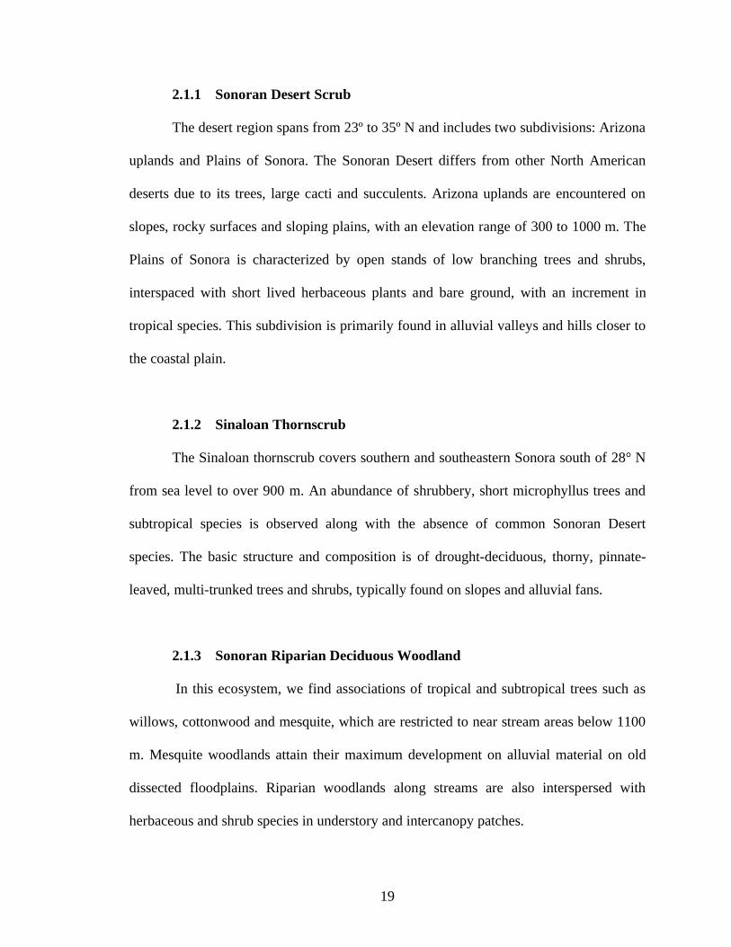
2.1.1 Sonoran Desert Scrub

The desert region spans from 23º to 35º N and includes two subdivisions: Arizona

uplands and Plains of Sonora. The Sonoran Desert differs from other North American

deserts due to its trees, large cacti and succulents. Arizona uplands are encountered on

slopes, rocky surfaces and sloping plains, with an elevation range of 300 to 1000 m. The

Plains of Sonora is characterized by open stands of low branching trees and shrubs,

interspaced with short lived herbaceous plants and bare ground, with an increment in

tropical species. This subdivision is primarily found in alluvial valleys and hills closer to

the coastal plain.

2.1.2 Sinaloan Thornscrub

The Sinaloan thornscrub covers southern and southeastern Sonora south of 28° N

from sea level to over 900 m. An abundance of shrubbery, short microphyllus trees and

subtropical species is observed along with the absence of common Sonoran Desert

species. The basic structure and composition is of drought-deciduous, thorny, pinnate-

leaved, multi-trunked trees and shrubs, typically found on slopes and alluvial fans.

2.1.3 Sonoran Riparian Deciduous Woodland

In this ecosystem, we find associations of tropical and subtropical trees such as

willows, cottonwood and mesquite, which are restricted to near stream areas below 1100

m. Mesquite woodlands attain their maximum development on alluvial material on old

dissected floodplains. Riparian woodlands along streams are also interspersed with

herbaceous and shrub species in understory and intercanopy patches.

20

2.1.4 Sonoran Savanna Grassland

These subtropical grasslands are encountered at elevations between 900 and 1000

m on flat plains and along large river valleys on deep, fine textured soils. This ecosystem

is commonly found in central and eastern Sonora. Tree and scrub components vary in

composition, with mesquite as the dominant tree and the presence of large cacti.

2.1.5 Madrean Evergreen Woodland

This ecosystem is found in the foothills and mountains of the Sierra Madre

Occidental. A large variety of oak species are present, including Chihuahuan oak and

Mexican blue oak. In northern Sonora, oak woodlands descend to about 1200 to 1350 m

in proximity to savanna grasslands, while in central and southern Sonora, this ecosystem

occurs as low as 880 to 950 m and borders Sinaloan thornscrub. Some cacti and leaf

succulents of the savanna grassland also extend into this ecosystem.

2.1.6 Madrean Montane Conifer Forest

These forests are encountered in higher plateaus and mountains of Sonora with an

elevation range from 2000 m to 3050 m, but more commonly from 2200-2500 m. The

most common tree species include white Mexican pine and Chihuahuan pine. The lower

limits of the conifer forest are in contact with Madrean evergreen woodland.

21

Figure 2.2: Regional cross-section with the distribution of the ecosystems. Elevation is expressed as meters above sea level.

2.2. Field and Remote Sensing Datasets

Ground-based precipitation and soil moisture observations were obtained from a

network of fifteen instrumentation sites installed during 2004 as part of SMEX04 (Vivoni

et al., 2007). Fig. 2.1 presents the locations of the continuous stations, with five sites in

the Río Sonora and ten sites in the Río San Miguel. Table 2.1 presents the station

locations, ecosystem classifications and elevations. Precipitation data (mm/hr) were

acquired with a 6-inch funnel tipping bucket rain gauge (Texas Electronics, T525I), while

volumetric soil moisture (%, in hourly intervals) was obtained at a 5-cm depth with a 50-

MHz soil dielectric sensor (Stevens Water Monitoring, Hydra Probe). The Hydra Probe

determines soil moisture by making high frequency measurements of the complex

dielectric constant in a 22 cm3 soil sampling volume. We used a factory calibration for

sandy soils to transform the dielectric measurement to volumetric soil moisture (%)

(Seyfried and Murdock, 2004).

22

Station

ID Ecosystem

Easting

[m]

Northing

[m]

Altitude

[m]

130 Sinaloan thornscrub 531465 3323298 720 131 Sinaloan thornscrub 532166 3317608 719 132 Sinaloan thornscrub 546347 3314298 900 133 Sinaloan thornscrub 539130 3305014 638 134 Madrean evergreen woodland 551857 3343293 1180 135 Sonoran riparian deciduous woodland 546349 3346966 1040 136 Sonoran desert scrub 532579 3353405 1079 137 Sonoran savanna grassland 571287 3312065 660 138 Sonoran savanna grassland 570690 3324453 726 139 Sonoran savanna grassland 568744 3336421 760 140 Sonoran savanna grassland 571478 3352076 1013 143 Sonoran riparian deciduous woodland 542590 3356533 960 144 Sonoran desert scrub 530134 3341169 800 146 Madrean evergreen woodland 551091 3315638 1385 147 Sinaloan thornscrub 544811 3290182 620

Table 2.1: Regional hydrometeorological station locations, altitudes and ecosystem classifications. The coordinate system for the locations is UTM 12N, datum WGS84.

Table 2.2 presents the limited amounts of missing data during the study period

due to equipment malfunction or data loss related to site inaccessibility during floods. We

also use observations from a 9-m eddy covariance tower deployed in a subtropical

scrubland near Rayón, Sonora at an elevation of ~630-m (Fig. 2.1). Measurements at the

tower include precipitation, net radiation and albedo (CNR-1 net radiometer), sensible

and latent heat flux (L17500 hygrometer, CSAT3 sonic anemometer), and soil moisture

and soil temperature at 5-cm depth (Stevens Vitel sensor). Data from the 2007 summer

season are used as these capture the monsoon transition. Half-hourly measurements were

aggregated to the daily scale to facilitate comparisons between pre-monsoon (DOY 151-

184) and monsoon (DOY 185-240) periods. More details on the sampling methods can be

found in Watts et al. (2007) and Vivoni et al. (2009).

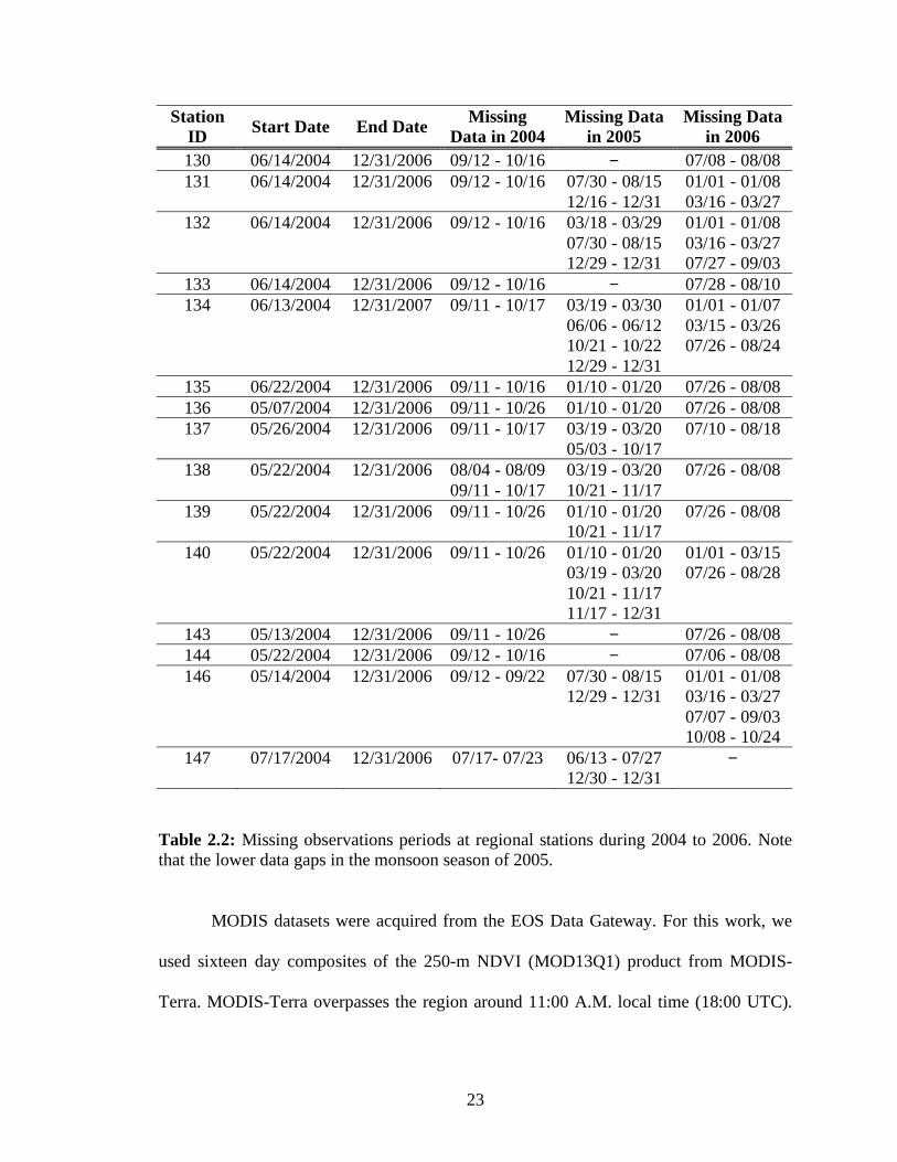
23

Station

ID Start Date End Date

Missing

Data in 2004

Missing Data

in 2005

Missing Data

in 2006

130 06/14/2004 12/31/2006 09/12 - 10/16 07/08 - 08/08 131 06/14/2004 12/31/2006 09/12 - 10/16 07/30 - 08/15 01/01 - 01/08

12/16 - 12/31 03/16 - 03/27 132 06/14/2004 12/31/2006 09/12 - 10/16 03/18 - 03/29 01/01 - 01/08

07/30 - 08/15 03/16 - 03/27 12/29 - 12/31 07/27 - 09/03

133 06/14/2004 12/31/2006 09/12 - 10/16 07/28 - 08/10 134 06/13/2004 12/31/2007 09/11 - 10/17 03/19 - 03/30 01/01 - 01/07

06/06 - 06/12 03/15 - 03/26 10/21 - 10/22 07/26 - 08/24 12/29 - 12/31

135 06/22/2004 12/31/2006 09/11 - 10/16 01/10 - 01/20 07/26 - 08/08 136 05/07/2004 12/31/2006 09/11 - 10/26 01/10 - 01/20 07/26 - 08/08 137 05/26/2004 12/31/2006 09/11 - 10/17 03/19 - 03/20 07/10 - 08/18

05/03 - 10/17 138 05/22/2004 12/31/2006 08/04 - 08/09 03/19 - 03/20 07/26 - 08/08

09/11 - 10/17 10/21 - 11/17 139 05/22/2004 12/31/2006 09/11 - 10/26 01/10 - 01/20 07/26 - 08/08

10/21 - 11/17 140 05/22/2004 12/31/2006 09/11 - 10/26 01/10 - 01/20 01/01 - 03/15

03/19 - 03/20 07/26 - 08/28 10/21 - 11/17 11/17 - 12/31

143 05/13/2004 12/31/2006 09/11 - 10/26 07/26 - 08/08 144 05/22/2004 12/31/2006 09/12 - 10/16 07/06 - 08/08 146 05/14/2004 12/31/2006 09/12 - 09/22 07/30 - 08/15 01/01 - 01/08

12/29 - 12/31 03/16 - 03/27 07/07 - 09/03 10/08 - 10/24

147 07/17/2004 12/31/2006 07/17- 07/23 06/13 - 07/27 12/30 - 12/31

Table 2.2: Missing observations periods at regional stations during 2004 to 2006. Note that the lower data gaps in the monsoon season of 2005.

MODIS datasets were acquired from the EOS Data Gateway. For this work, we

used sixteen day composites of the 250-m NDVI (MOD13Q1) product from MODIS-

Terra. MODIS-Terra overpasses the region around 11:00 A.M. local time (18:00 UTC).

24

In the other hand, MODIS-Aqua overpasses the same area at 12:00 P.M. local time

(19:00 UTC). For each overpass, the NDVI is calculated from reflectance as:

NDVI = NIR red

NIR + red

, (2.1)

where NIR and red are the surface bidirectional reflectance factors for MODIS bands 2

(841-876 nm) and 1 (620-670 nm), respectively. The advantage of MODIS vegetation

indices is that they rely on the level 2 daily surface reflectance product (MOD09), which

it is corrected for external factors such as molecular scattering (Raleigh scattering), ozone

absorption and aerosols (Vermote et al., 2002). A more complex effect on the degradation

of NDVI is caused by topographic variation, including effects of shadow, adjacent hill

illumination, sky occlusion and slope orientation. However, MODIS vegetation indices

eliminate or significantly reduce topographic effects by three different approaches: 1) by

the band ratio concept of NDVI that reduces many forms of noise (including illumination

differences, cloud shadows, atmospheric attenuation and certain topographic variations).

Matsushita et al. (2007) found that MODIS NDVI is not affected by topographic

variations considering its ratio format, while EVI is very sensitive to topographic

conditions because it is not expressed as a function of ratio vegetation index and is using

the soil adjustment factor “L”. 2) The standardization of sun-surface-sensor geometries

with bidirectional reflectance distribution function (BRDF) models. The BRDF is a

mathematical description of the optical behavior of a surface with respect to angles of

illumination and observation. Description of BDRFs for actual surfaces permits

assessment of the degrees to which they approach the ideals of specular (anisotropic

reflection) and diffuse (isotropic reflection) surfaces (Campbell, 2007). 3) The moderate

25

spatial resolution of MODIS reduces the effects of topography because within one pixel

are of 62,500 m2, a larger samples of slopes and illumination conditions are aggregated

(Burgess et al., 1995). The main purpose of compositing over the 16-day periods is to

select the best observation, on a per pixel basis, from all the retained data. The MODIS

vegetation index compositing algorithm utilizes three main components as shown in

figure 2.3: (1) Maximum Value Composite (MVC), (2) Constrained-View angle

Maximum Value Composite (CV-MVC) and (3) BRDF-C: Bidirectional reflectance

distribution function composite. The technique employed depends on the number and

quality of observations. The MVC selects the pixel observation with the highest NDVI to

represent the compositing period (Holben, 1986). A disadvantage of the MVC approach

is that it selects pixels with NDVI values greater than the nadir value. The CV-MVC and

BRDF methods compositing techniques are designed to constrain the angular variations

of the MVC selection method. These latter methods compare the two highest NDVI

values and select the observation closest to nadir view to represent the composite. This

helps to reduce the spatial and temporal discontinuities in the composite. Finally, the

BRDF method uses all bidirectional reflectance observations with acceptable quality to

interpolate to their nadir-equivalent band reflectance values. With these reflectance

values, then NDVI or EVI is calculated. The BRDF model used in MODIS is the

Walthall semi-empirical BRDF model.

( ) cba svvvvvsv ++= )cos(,, 2 , (2.2)

where is the atmospherically corrected reflectance in band , v is the satellite view

zenith angle, v is the satellite view azimuth angle, s is the solar azimuth angle, and c ,

b , c are model parameters coefficients.

26

Figure 2.3: Diagram of MODIS compositing method. Taken from Huete et al. (2002).

The model is fitted to the observations by a least squares procedure on per-pixel basis to

estimate nadir view equivalent reflectances (c ). At least five good quality observations

( v 45°) after initial screening process are required for model inversion. (Huete et al.,

2002).

MODIS land surface temperature is derived from thermal infrared data using

bands 20 (3.660-3.840 μm), 22 (3.929-3.989 μm), 23 (4.020-4.080 μm), 26 (1360-1390

nm), 29 (8.400-8.700 μm), 31 (10.780-11.280 μm), 32 (11.770-12.270 μm) and 33

(13.185-13.485 μm). The LST/Emissivity algorithms use MODIS data as input, including

geolocation, radiance, cloud masking, atmospheric temperature, water vapor, snow, and

land cover (Wang, 1999). For this study, we used eight-day composites with a spatial

resolution of 1 kilometer (MOD11A2) for the same time period as NDVI datasets.

27

The MODIS Bidirectional Reflectance Distribution Function (BRDF)/Albedo

products describe how land surfaces appear under perfect scattering conditions without

the influence of view angle. The BRDF/Albedo algorithm relies on multi-date,

atmospherically corrected, cloud-cleared data and a semiempirical kernel-driven

bidirectional reflectance model to determine a global set of parameters describing the

BRDF of the land surface (Schaaf et al., 2002).

For this study, we used a sixteen-day white sky albedo composite, which is

defined as albedo in the absence of a direct component when the diffuse component is

isotropic, with a spatial resolution of 1 km (MOD43B3). Each of the MODIS images was

mosaicked, clipped and reprojected using the HDF-EOS to GIS Format Conversion Tool

(HEG tools version 2.8). This tool allows reprojection from the native MODIS

Integerized Sinusoidal (ISIN) grid to the Universal Transverse Mercator (UTM) Zone

12N projection used in our analysis. Figure 2.4 shows an example of a MODIS scene that

was reprojected using HEG tools. In addition to the reprojection, this tool allows to cut

the entire MODIS scene into a smaller domain. This software also allows converting the

native MODIS HDF data format (Hierarchical Data Format) into a GEOTIFF image, a

format that is widely used in most image processing software.

To minimize the effect of human-impacted regions, we created a mask excluding

zones with minimal NDVI changes over time (e.g., mines, urban areas and water bodies),

thus focusing our analysis to areas of natural vegetation. All datasets encompass 83

images from January 2004 to June 2007, with a domain size of ~198 by 265 kilometers

overlying the study region (Fig. 2.5).

28

Figure 2.4: Reprojection of MODIS image using HEG tools conversion software: (a) Original MODIS sinusoidal projection. (b) UTM projection using WGS-84 datum.

Figure 2.5: (a) Masked image excluding water bodies, urban areas and mines. These black-colored regions have NO DATA value. (b) Final product by multiplying the masked image with the clipped and projected EVI or NDVI image.

2.3. Metrics of Spatial and Temporal Vegetation Dynamics

In the following, we describe analyses conducted to quantify the seasonal and

interannual vegetation dynamics. Remotely-sensed NDVI data were characterized

through: (1) analysis of temporal variations at each continuous station; (2) derivation of

29

vegetation metrics; (3) analysis of time stability of the spatiotemporal fields; and (4)

identification of elevation controls on the vegetation statistics along two transects.

2.3.1 Temporal Variation of Vegetation Metrics

Temporal evolution of vegetation dynamics is important because it is an indicator

of climate parameters such as temperature, solar radiation and precipitation. For example,

knowing when the vegetation greening begins is an indication of the onset of NAM.

Interannual variability of climatic variables can also be identified with long-term

observations. In this particularly case, the use of remote sensing techniques allow land

surface observations at regional scale at analysis of spatial, temporal and spectral

patterns. In addition, these patterns can be measured, described and correlated with other

information (like ground information or another source of ancillary data). Therefore, this

technique has more advantages than conventional methods like field surveying.

Temporal variations at specific sites were obtained by determining the mean and

standard deviation of NDVI for each MODIS composite image from the 3 3 pixel (750

x 750 m) domain around a station. The arithmetic mean provides the averaged conditions

at a site and accounts for uncertainties in the georeferencing of the station and MODIS

image. The standard deviation captures the spatial variability around an instrument site.

Figure 2.6 shows how the mean value of 250 m resolution MODIS products was

obtained.

Temporal variations of NDVI were then used to estimate a set of vegetation

metrics using the methods of Lloyd (1990) and Reed et al. (1994). In order to extract the

vegetation metrics, we applied a smoothing method to the raw NDVI time series using a

30

Figure 2.6: Extraction of pixel values. The red dot represents the station location and the pixel beneath the location is considered the central pixel. Then for the estimation of the mean value, we took into consideration the eight values around the central pixel.

LOESS regression. The name LOESS is derived from the term “locally weighted scatter

plot smooth” because the method uses a locally weighed linear regression to smooth the

data. The method is considered local because, like the moving average method, each

smoothed value is determined by neighboring data points defined within the span. The

process is weighted because a regression weight function is defined for the data points

contained within the span. Finally, this smoothing process uses a quadratic polynomial

model. (Mathworks, 2004). The main goal of the smoothing process is to reduce the

effects of outliers and preserve the essential features of the NDVI variations.

With the smoothed NDVI time series, we generated two different lagged time

series which we have applied to different moving averages following Reed et al. (1994):

(1) A backward moving average (BMA) was applied to the first lagged time series in

reverse chronological order and it was overlapped to the original smoothed NDVI time

31

series; and (2) a forward moving average (FMA) was applied to the second lagged time

series in forward direction and overlapped again to the original smoothed NDVI time

series. The two lagged time series were subsequently lagged by 3 time periods, each 16

days in length, to detect the crossing properties of the NDVI time series (e.g., timing of

vegetation greening and senescence). The intersection between the forward lagged time

series curve and the original smoothed NDVI time series curve is considered the point

where the photosynthetic activity of vegetation starts. Conversely, the intersection

between the backward lagged time series curve and the original smoothed NDVI curve is

considered the point where the senescence of vegetation starts.

We tested the sensitivity of the method to different lag lengths to best match the

annual NDVI cycle in the study region. Based on the above, we found the beginning of

the vegetation greening as the crossing between the smoothed NDVI and the FMA.

Similarly, the end of the greening season was found as the crossing between the

smoothed series and the BMA. Fig. 2.7a is an example of the original NDVI data, the

smoothed series and moving averages. Once the start and end of the greening are found,

several vegetation metrics can be estimated (Reed et al., 1994): (1) Duration of

Greenness (days), defined as the period between the onset and end of the greenness; (2)

Growing season integrated NDVI (iNDVI, dimensionless), measured as the area under

the smoothed NDVI series; (3) Seasonal range of NDVI ( NDVI, dimensionless) simply

determined as the difference between the maximum seasonal (NDVImax) and minimum

seasonal (NDVImin) NDVI values; and the (4) Rate of Greenup and the (5) Rate of

Senescence, defined as the change in NDVI per time (day-1) for the beginning and end of

the greening season, respectively.

32

Figure 2.7: Determination of vegetation metrics. (a) Identification of the beginning and end of the vegetation greening using the smoothed NDVI series and the backward (BMA) and forward (FMA) moving averages for station 130 (Sinaloan thornscrub). The original NDVI data is represented by the open circles. (b) Example of the vegetation metrics (iNDVI, NDVI, Rate of Greenup, Rate of Senescence and Duration of Greenness) for station 130 during the 2004 season.

33

One simple way to estimate the Rate of Greenup is to calculate the slope between

the point of vegetation green up and the maximum seasonal NDVI (NDVImax). In the case

of Fig. 2.7b presents an example of the determination of the vegetation metrics for a

Sinaloan thornscrub site during the 2004 growing season.

Sensitivity to the selection of the time periods was performed in order to assess

the impact on the vegetation metrics. We changed the number of lagged days in the

forward moving average (FMA) and the backward moving average (BMA) in order to

establish the starting point of photosynthetic activity and the ending point of plant

activity (senescence). We compared the results using 2, 3, 4, 5, 6 and 7 lagged time

periods and how they affect the calculation of iNDVI or iEVI (the area under the curve).

The sensitivity analysis was done for the year 2005 at station 132. Figure 2.8 shows the

results for FMA in order to get the beginning of greening season. As observed, the

beginning of growing season starts between time period 33 or 34. The difference is not

large among the number of lagged periods. Figure 2.9 shows the result for modifying the

number of lagged days in the BMA. Vegetation senescence lies between time period 49

and 51, hence difference in ending season point is not large. Table 2.3 shows the

comparison among different lagged time periods and their influence in the estimation of

iEVI (area under the time series curve of EVI). The iEVI is slightly affected by the

change in starting and ending point selection. The largest difference is around 6% in iEVI

values with 4 and 5 lagged time periods. Conversely, low difference of 3% occurs

between areas values with 2 and 6 lagged time periods.

34

Figure 2.8: Sensitivity analysis for Forward Moving Average (FMA).

Figure 2.9: Sensitivity analysis for Backward Moving Average (BMA).

35

Table 2.3: Comparison among different lagged time periods and their influence in the estimation of time integrated EVI (iEVI).

2.3.2 Spatial and Temporal Analysis: The Time Stability Concept

To analyze the temporal and spatial variability of NDVI, albedo and LST, we

applied the concepts of spatial and temporal persistence (e.g., Vachaud et al., 1985;

Mohanty and Skaggs, 2001; Grant et al., 2004; Jacobs et al., 2004; Vivoni et al., 2008a).

We quantified the spatial and temporal root mean square error (RMSE) of the mean

relative difference ( ) for each MODIS pixel during the study period. This analysis is

important because it allows us to perform statistics of the spatial and temporal

distributions of the land surface processes, as well as, identifying locations with temporal

and spatial persistence. Basically, the persistence is captured by the mean relative

difference that evaluates the difference between a specific location and the temporal or

spatial mean. With the spatial stability, we can estimate locations that capture the basin-

average conditions in NDVI, LST and albedo. Conversely, the temporal persistence

identifies locations that show high or low seasonality.

Lagged 16-Days time periods

Starting 16-Day Period

Ending 16-Day period Area

2 33.30 48.70 4.21

3 33.45 49.00 4.21

4 33.65 50.70 4.47

5 33.85 50.90 4.47

6 34.00 50.94 4.32

7 34.05 50.98 4.32

36

Figure 2.10: Temporal evolution of the mean spatial NDVI and surface albedo during the study period. Every point in the plot represents a mean spatial value used to estimate the spatial RMSE of the difference.

Figure 2.11: Temporal mean NDVI, surface albedo and land surface temperature used to estimate the temporal RMSE of the difference. Every images is the result of averaging 83 MODIS composite images.

37

The main difference between the spatial and temporal RMSE is the mean value

used to compute the relative difference. In the case of the spatial RMSE s, we used the

spatial mean of each image and calculated the difference between every pixel and the

spatial mean. Figure 2.10 shows the mean spatial values for NVDI and albedo used to

estimate the spatial RMSE . Every point in the plot represents one mean value in the

regional domain and was subtracted from all pixels per MODIS scene. Conversely, for

the temporal RMSE t, we used the temporal mean for each pixel over all images and

then calculated the difference between each pixel and its temporal mean. Figure 2.11

shows the temporal mean for NDVI, LST and albedo used to estimate the temporal

RMSE for the study period.

To compute the spatial RMSE s, we first calculated the spatial mean of the

parameter of interest in the region for each MODIS composite as:

X sp,t =1

nXs,t

s=1

n

, (2.3)

where tspX , is the spatial mean for the MODIS parameter (NDVI, albedo or LST) for

each date (t) over all pixels (s) and n is the total number of pixels (i.e., 992,450 pixels,

863 1150). Using this method, we obtained 83 spatially-averaged MODIS values.

Conversely, the temporal mean of MODIS parameter in each pixel is computed as:

X tm,s =1

Nt

Xs,tt=1

Nt

, (2.4)

where stmX , is the temporal mean of the MODIS parameter and Nt is the total number of

processed MODIS images (83 in total). In (2) and (3), tsX , is the MODIS parameter value

for pixel (s) at time (t). The mean relative difference captures the difference between a

38

pixel and the mean (spatial or temporal) for all MODIS parameter images. In the spatial

case, the mean relative difference s is computed as:

s =1

Nt

Xs,t X sp,t

X sp,tt=1

Nt

. (2.5)

In addition, the temporal mean relative difference t is computed as:

t =1

Nt

Xs,t X tm,t

X tm,tt=1

Nt

. (2.6)

The variances of the relative difference ( t( )2 for temporal and s( )

2for spatial cases)

are:

( )2

1 ,

,,2

1

1

=

=tN

t

stsp

tspts

t

sX

XX

N, and (2.7)

( )2

1 ,

,,2

1

1

=

=tN

t

tttm

ttmts

t

tX

XX

N . (2.8)

Finally, the root mean square error of the mean relative difference (RMSE ) is a

single metric which captures both the bias and the spread around the bias (Jacobs et al.,

2004). It is computed here for the temporal and spatial cases as:

( )( )2122 sssRMSE += , and (2.9)

( )( )2122 tttRMSE += . (2.10)

Low sRMSE sites are stable pixels that closely track the spatially-averaged

conditions in the region over time. This metric can identify ecosystems that capture the

temporal surface conditions for a region. We would expect ecosystems that dominate the

regional greening, such as the Sinaloan thornscrub, would exhibit low sRMSE . On the

39

other hand, low tRMSE indicates pixels with values close to the temporal mean at the

site. This metric indicates ecosystems that have more limited seasonal changes.

We expect that ecosystems, such as the Madrean evergreen woodland with lower

seasonality, would exhibit low tRMSE . RMSE values range from 0 to 1, with values

near zero having high persistence. Thus, spatial RMSE near zero represents pixels that

closely track the spatial mean of the region (and vice-versa). In the case of temporal

RMSE , values near zero are sites that exhibit low temporal variations (and vice-versa).

2.3.3 Elevation control on Vegetation Statistics

Few studies in the region have addressed the potential interactions between the

monsoon system and land surface properties as topography. Vivoni et al. (2007) found

that topography exerted a strong control on the spatial and temporal variability in soil

moisture, with distinct landscape regions experimenting different hydrologic regimes.

Gochis et al. (2004) showed important terrain control on the distribution of precipitation

using rain gauge observations along topographic transects in the Sierra Madre Occidental.

The authors found that at high elevations, summer precipitation was more frequent but

with lower intensity, meanwhile, lower elevations showed less frequency but higher

intensity. This suggests that topography controls the diurnal cycle of convection. Because

NDVI is strongly correlated with precipitation, we can infer surface hydrological

conditions by observing the temporal evolution of vegetation indices along a topographic

transect.

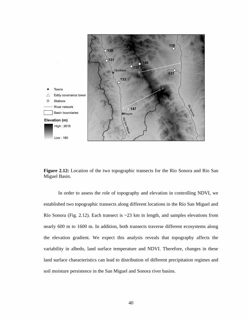
40

Figure 2.12: Location of the two topographic transects for the Rio Sonora and Rio San Miguel Basin.

In order to assess the role of topography and elevation in controlling NDVI, we

established two topographic transects along different locations in the Río San Miguel and

Río Sonora (Fig. 2.12). Each transect is ~23 km in length, and samples elevations from

nearly 600 m to 1600 m. In addition, both transects traverse different ecosystems along

the elevation gradient. We expect this analysis reveals that topography affects the

variability in albedo, land surface temperature and NDVI. Therefore, changes in these

land surface characteristics can lead to distribution of different precipitation regimes and

soil moisture persistence in the San Miguel and Sonora river basins.

41

2.4. Relationships between NDVI, Precipitation and Soil Moisture

Several approaches were pursued to explore the relations between NDVI,

precipitation and soil moisture. A linear regression between vegetation greening and

precipitation was carried out using iNDVI and accumulated seasonal rainfall. Due to

sampling gaps, this analysis was focused on the 2005 monsoon. In order to assess the

efficiency of the ecosystems to express plant growth and biomass production with

precipitation, we used the Greenness-precipitation ratio (GPR), which is analogous to the

Rain Use efficiency (RUE). The original RUE equation was proposed by Le Horeau

(1994):

RUE =ANPP

R , (2.11)

where ANNP is the aboveground net primary productivity and R is the seasonal

precipitation. Paruelo et al. (1997) found that ANPP is closely related to time integrated

NDVI. This author explored the relationship for the central grassland region in United

States and it is expressed as an exponential function:

ANPP = 3803 iNDVI1.9028. (2.12)

The functional relation from Paruelo et al. (1997) suggests that iNDVI is related to

rainfall use efficiency. Based on this we developed a relation between GPR and iNDVI

from our datasets:

100=seasonR

iNDVIGPR , (2.13)

where iNDVI is the time integrated NDVI during the growing season and Rseason is the

accumulated rainfall during the growing season. The goal of multiplying the ratio by 100

is to produce GPR values greater than 1 and make them easier to compare.

42

In addition, we calculated correlation coefficients between NDVI and accumulated

rainfall and time-averaged soil moisture in the current and previous months using a

combination of different monthly lags for 2005.

2.5. Cluster Analysis and Unsupervised Classification

Time stability analysis can be used to identify patterns in land surface conditions

and group these into zones with similar behavior. We performed an unsupervised

classification using the spatial and temporal RMSE of the three land surface variables

(NDVI, albedo, LST) as input fields. Before the unsupervised classification, we

performed a cluster analysis, which returns naturally occurring groupings in the data

based on multivariate statistics. The cluster analysis results were subsequently used to

perform a maximum likelihood classification (MLM) that calculates the probability of the

cell belonging to that class given its attribute values (e.g., Campbell, 2007). Through this

analysis, we identify classes representing different land surface dynamics. In this case,

the classes are grouped by high or low seasonality in NDVI, albedo and LST, as well as,

high or low spatial representation of the region. As a result, the classes are distinct

functional groups capturing different land surface responses. Functional groups

occupying large spatial domains and exhibiting significant seasonal changes in LST,

albedo and NDVI are expected to have higher potential contributions to a vegetation-

rainfall feedback mechanism. The optimum number of functional groups will be

determined based on the highest accuracy obtained by comparing the resulting functional

group map with a reference map. In this thesis, we will use a land cover map generated

by Yilmaz et al. (2008) of the region as reference image. The classification accuracy will

43

be determined using an error matrix and by comparing around 10,000 randomized points

between the new functional group map and the reference image.

44

CHAPTER 3

RESULTS AND DISCUSSION

In the following, we present the set of spatial and temporal analyses used to

quantify the vegetation dynamics in the study region and relate these to metrics that

quantify the precipitation and soil moisture observations from the regional network. Our

focus is primarily on the regional characterization of vegetation dynamics afforded by the

remote sensing data, with more detailed study at representative stations of particular

ecosystems arranged along topographic transects. In addition, we present the results of

the cluster analysis by using RMSE as input in order to demonstrate that the eddy-

covariance tower in the region in located in a functional group that closely tracks the

regional spatial mean with high seasonality in NDVI, albedo and LST. Finally, we show

time series at eddy-covariance tower demonstrating the highly coupled relation between

soil moisture conditions, vegetation green up and land surface processes. These changes

in surface conditions during monsoon transition show evidence for a potential land

surface-atmosphere feedback mechanism that can promote convective rainfall.

3.1. Spatial and Temporal Vegetation Dynamics in Regional Ecosystems

Vegetation conditions in the regional ecosystems are assessed to determine the

seasonal and interannual variations induced by differing amounts of NAM precipitation

and soil moisture. Fig. 3.1 presents the seasonal change in NDVI (DNDVI = (NDVImax–

NDVImin)/NDVImin, expressed as a percentage) for the three monsoons (2004 to 2006).

45

Figure 3.1: Comparison of seasonal NDVI change (%). The percentage of NDVI change is calculated using the lowest and highest NDVI for a particular summer season (2004 to 2006). sR is the total summer rainfall (July to September) averaged over all stations.

There is an evident variation in the spatial pattern of DNDVI related to ecosystem

distributions, terrain characteristics and rainfall amounts. The spatial distribution of

DNDVI and its range varies for each year, following the total rainfall averaged over all

regional stations ( sR ) from July to September. In the year 2004 ( sR = 251 mm), the

largest degree of vegetation greening occurs in the southeastern part of the domain,

outside the regional network. Nevertheless, the region between stations 146 and 147 in

the Río San Miguel exhibited high greening, in agreement with the elevated soil moisture

observed from aircraft-based retrievals (Vivoni et al., 2008a). In contrast, the year 2005

was the driest in the record ( sR = 222 mm) and as a result experienced the smallest

DNDVI, with a range from 50 to 150%. Note, however, that isolated patches experience

high degrees of greening, suggesting localized storms during this monsoon. Conversely,

the year 2006 exhibited the largest change in NDVI due to the elevated precipitation

46

( sR = 350 mm). The spatial distribution of DNDVI is also more uniform in the region,

ranging from 200 to 300%, indicating that the overall ecosystem response was vigorous

and spatially extensive. Interestingly, small changes in seasonal NDVI are always

observed in forested riparian corridors (Sonoran riparian deciduous woodland) and high

altitude mountains (Madrean montane conifer forests) as these remain green throughout

the year. Overall, the spatial NDVI fields indicate seasonal and interannual changes

linked to rainfall, ecosystem pattern and topography.

Fig. 3.2 presents the temporal variations of NDVI, precipitation and soil moisture

over the period January 2004 to June 2007 (at 16-day intervals) at four regional stations:

(a) station 146 (Madrean evergreen woodland), (b) station 132 (Sinaloan thornscrub), (c)

station 139 (Sonoran savanna grassland), and (d) station 144 (Sonora desert scrub). The

four stations were selected to represent different ecosystems as well as the changes in

hydrologic conditions along elevation gradients (see Table 2.1 for station descriptions).

For each site, hourly precipitation and soil moisture observations were accumulated or

averaged, respectively, over the 16-day intervals to match the MODIS compositing

period. Remotely-sensed NDVI time series are depicted as the station mean (symbols)

and ±1 standard deviation (error bars) over a 3 3 window (250-m pixels) around the

station. Any data gaps in the ground or remotely-sensed observations resulted in the

removal of the composites and are shown as broken lines (see Table 2.2 for data gaps).

The temporal variations in vegetation greenness, as captured by the station NDVI,

are dramatic in each ecosystem and closely related to the hydrologic conditions at each

site. The Madrean evergreen woodland (Fig. 3.2a) exhibited the highest precipitation of

the ecosystems in the region, with an exceptional rainfall in 2006 (up to 300 mm in July).

47

Figure 3.2: Temporal variation of NDVI among different regional ecosystems: (a) Madrean evergreen woodland (station 146), (b) Sinaloan thornscrub (station 132), (c) Sonoran savanna grassland (station 139), and (d) Sonoran desert scrub (station 144). NDVI symbols correspond to the average value calculated in the 3 3 pixel region around each station for each composite. The vertical bars depict the ±1 standard deviation of the 3 3 pixel region. Precipitation (mm) is accumulated during 16-day intervals and shown as gray bars, while the averaged surface volumetric soil moisture (%) during the 16-day periods is shown as open circles.

48

In response, soil moisture was elevated in the 2006 summer, reaching >20% in the

surface soil layer. This plant-available water led to a vigorous summer greening reflected

in a peak NDVI of nearly 0.8. Similar summer processes are observed in station 146 for

2004 and 2005, albeit with lower precipitation, soil moisture and peak NDVI. In contrast,

the Sinaloan thornscrub (Fig. 3.2b) showed less rainfall than higher sites, but more

consistent greening in the different summers. The NDVI range (~0.25 to ~0.8) varied

slightly across the different monsoons, suggesting this ecosystem is fairly resilient to

hydrologic changes. Sonoran savanna grasslands (Fig. 3.2c) have a more muted

vegetation response (smaller NDVI range) as compared to the other ecosystems.

Nevertheless, the station NDVI exhibits high temporal variations in response to wet and

dry periods, including a spring peak in 2005 after a wet winter. Finally, the Sonoran

desert scrub (Fig. 3.2d) also experiences summer greening, with relatively small year-to-

year variations in response to variations in rainfall and soil moisture. Interestingly,

summer 2005 had more favorable hydrologic conditions than 2006 at this station and thus

the highest peak NDVI in the three-year record.

It is important to mention that NDVI values during the dry season never reached

values near zero which it is commonly identified as scarce vegetation. We have observed

that the dynamic range of vegetation in the region varies between 0.2 and 0.8. However,

Huete et al., 2002; found that the dynamic range of MODIS NDVI varies from about 0.05

to nearly 0.9 using as reference different ecosystems in the world. The highest value of

NDVI were found in the broadleaf Harvard forest (Massachusetts), while the minimum

NDVI value was measured in the hyper-arid sites located in the Atacama and Uyuni

49

deserts (LAI = 0). These latter sites were considered as zero baselines for vegetation

indices values. However, it is important to mention that the NDVI values for MODIS

NDVI baseline (bare soil) never fell below 0. Furthermore, Huete et al. (2002) compared

MODIS NDVI values with NDVI values from AVHRR. He found that MODIS NDVI is

signicantly higher than those from AVHRR resulting in greater seasonal dynamic range

for all sites he analyzed. Furthermore, Buheaosier et al. (2003) compared MODIS NDVI

with other sensors on broad leaf forest. They found that NDVI derived from MODIS is

the largest followed by those of ETM (landsat), ASTER and AVHRR (see table 3.1). In

addition, MODIS showed the largest minimum, mean and maximum numerical values

while ASTER showed the opposite characteristics. The reason why the values of NDVI

are higher in MODIS can be caused by the influence of water vapor content in the

atmosphere, which strongly affects the reflectance values in the NIR band of other

sensors, especially AVHRR; causing NDVI values to decrease. The narrower MODIS-

NIR infrared band (see table 3.1) avoids the water absorption regions of the spectrum and

it was nearly unaffected by variations in water vapor content in the atmosphere.

Furthermore, the higher sensitivity of MODIS-NDVI may also be attributed to increased

chlorophyll sensitivity in the MODIS red band (Gitelson & Kauffman, 1998) and the

compositing method.

Fig. 3.2 also allows inspection of vegetation response in the three winter seasons,

receiving smaller and more variable rainfall amounts (e.g., Sheppard et al., 2002; Nagler

et al., 2007). While this is not the primary focus of this study, it is important to highlight

these variations. A relatively wet winter in 2005 impacted vegetation dynamics in two

ways:

50

Band Width (μm) Sensor

Red NIR ASTER 0.63-0.69 0.76-0.86 ETM+ 0.63-0.69 0.75-0.90 MODIS 0.62-0.67 0.84-0.88 AVHRR 0.58-0.68 0.72-1.00

Table 3.1: Comparison of the red and infrared bands for several remote sensing sensors. Taken from Buheaosier et al. (2003). (1) Maintaining green conditions for a longer period of time, or (2) leading to spring

season plant growth. In contrast, a relatively dry winter in 2006 caused a significant

decrease in NDVI in spring and early summer for all ecosystems. The linkages between

winter and summer precipitation, soil moisture and vegetation greening is of considerable

importance and has not been addressed in the region.

3.2. Quantifying Ecosystem Dynamics Through Vegetation Metrics

Vegetation metrics can aid in the quantification of ecosystem responses to the

precipitation and soil moisture during the North American monsoon. Table 3.2 presents

the phenological metrics obtained for each regional station during the monsoon seasons

in 2004 to 2006. Overall, the various metrics, in particular the iNDVI and NDVI,

confirm that summer 2006 had the most dramatic vegetation greening in most of the

regional stations. In contrast, stations during summer 2004 exhibited the shortest

Duration of Greenness and Days to NDVImax as well as the smallest iNDVI and NDVI.

51

Table 3.2: Comparison of vegetation metrics for the regional stations during the three monsoons.

52

The metrics also reveal differences and similarities in vegetation productivity

among the regional stations. For example, although stations 130, 131, 132, 133 and 147

are located in the same ecosystem (Sinaloan thornscrub), we can see differences in

productivity and the vegetation metrics. Station 132 obtained the highest vegetation

metrics among the stations located in Sinaloan thornscrub. This can be attributed to its

location in the foothills of Sierra Los Locos (elevation 900 m) and the influence of higher

precipitation and soil moisture conditions. The other stations fluctuate in elevation

between 620-730 m and have lower precipitation resulting in lower soil moisture. In

addition, these stations are located in the floodplain of the Rio San Miguel and have

experienced larger modifications in land cover. It is common to observe native vegetation

replaced by agriculture, resulting in an important decrease in vegetation metrics.

Another example of differences in the same ecosystem can be seen in stations 134

and 146, both located in Madrean evergreen woodland. Station 134 (elevation 1134 m)

showed lower vegetation metrics as compared to station 146 (elevation 1385 m).

Differences in vegetation metrics can be attributed to anthropogenic modifications. At

station 134, the oak forest stand has been impacted by introduced pasture for cattle.

Conversely, station 146 is not very accessible, although livestock activity has been seen

near the station. We also expect more rainfall because of the higher elevation.

Finally, riparian zones have been seriously impacted by human activities. While

we expect to see high vegetation productivity in these areas, their metrics values are as

low as grasslands. Among the factors that can influence the reduction in riparian zones

are deforestation, replacement of woodland by pastures, and decreases of water table

height impacting riparian vegetation access to groundwater. Long-term observations from

53

remote sensing would be needed to more carefully evaluate land use changes with time

and the impact of anthropogenic activities.

As observed in Fig. 3.2, the ecosystem composition at each site has a strong

control on the vegetation metrics for the different years. Stations with common plant

communities share similar response to summer rainfall. For example, lower productivity

stations are all in Sonoran savanna grasslands (stations 137, 138, 139) with low iNDVI,

NDVI and Duration of Greenness. Similarities are also observed in vegetation metrics

for stations in the Sonoran riparian deciduous woodland (stations 135, 143). For the wet

2006 summer, however, precipitation amount and soil water availability lead to certain

degrees of homogenization in the vegetation response across different ecosystems. For

instance, Madrean evergreen woodlands (station 146) and Sinaloan thornscrub (station

132) share similar responses to the 2006 NAM precipitation (e.g., iNDVI = 8.69 and 8.68

for 2006, respectively), despite having different plants and ecophysiological processes.

To explore this further, Table 3.3 presents temporal coefficients of variation

(CVs) for each vegetation metric computed for the average conditions in each ecosystem

across all years. As a result, the CV primarily captures the interannual variations in

vegetation metrics in a particular ecosystem. Ecosystems with high CVs imply large

interannual changes in the 2004 to 2006 summer monsoons. Note that Sonoran savanna

grassland and Sonoran riparian deciduous woodlands exhibit higher CVs for iNDVI,

NDVI and Duration of Greenness, indicating strong variations between years. Small CV

in iNDVI and high CV in NDVI is observed in the Sonoran desert scrub, suggesting this

ecosystem varies primarily in the NDVI range from year-to-year.

54

Coefficient of Variation (CV) Ecosystem

N iNDVI NDVImax NDVImin NDV

I

Duration of

Greenness

Days to

NDVImax

Madrean evergreen woodland 2 0.19 0.17 0.15 0.22 0.13 0.33 Sinaloan thornscrub 5 0.20 0.12 0.12 0.14 0.21 0.47 Sonoran savanna grassland 4 0.30 0.17 0.09 0.28 0.24 0.20 Sonoran desert scrub 2 0.09 0.35 0.35 0.30 0.41 0.46 Sonoran riparian deciduous forest 2 0.21 0.26 0.30 0.31 0.41 0.50

Table 3.3: Coefficient of variation (CV) of vegetation metrics for different ecosystems during the period 2004-2006. CV is calculated as the temporal standard deviation divided by the temporal mean averaged over all stations in each ecosystem (N sites in each ecosystem).

The Madrean evergreen woodland and Sinaloan thornscrub have intermediate

CVs for the vegetation metrics that appear to offset each other. For example, in the

Madrean evergreen woodland, CV in iNDVI is lower than the Sinaloan thornscrub, while

CV in NDVI is higher. This suggests that different ecosystems in the region respond in

variable ways to interannual hydrologic changes. Evergreen woodlands appear to vary

their maximum greening ( NDVI) in response to increased rainfall amounts, while

deciduous trees and shrubs vary the total productivity (iNDVI) during the growing

season. These two plant greenup strategies may explain how these ecosystems exist at

different elevation in the region. Finally, the vegetation metric with the highest year-to-

year variation is Days to NDVImax, indicating that the rate of ecosystem greening is

highly influenced by rainfall amounts during the monsoon onset.

3.3. Relations Between Vegetation and Hydrologic Indices

To further explore the relation between ecosystem dynamics and the precipitation

and soil moisture conditions, we compared iNDVI, the greenness-precipitation ratio

(GPR = [iNDVI/Rs]*100) and the total precipitation (Rs) at each station for the 2005

55

monsoon (Table 3.4). This particular summer was selected due to its limited amounts of

missing data in the regional stations. Fig. 3.3 presents a linear relation between iNDVI

and precipitation (Rs) at the 12 stations with complete data. The linear regression between

iNDVI and Rs results in (r2 = 0.64) with the regression line passing through the origin:

iNDVI = 0.021Rs. (3.1)

Conversely when the regression line was not forced to pass through the origin, the

equation slightly changes in the following way:

iNDVI = 0.025Rs -1.036. (3.2)

We noticed that the change in slope is hardly observable, hence; we can use either

formulas. However, we consider that is more correct to use equation 3.1 because we

expect to see no increment in biomass production (iNDVI) with zero units of rainfall.

Furthermore, in the case of equation 3.2, with a seasonal accumulated rainfall of 54.4 mm

we have an iNDVI value of zero. We do not have enough information to assume that this

value of precipitation is a threshold in vegetation productivity in the region.

Clearly, as rainfall amounts increase across the regional stations, ecosystem

productivity during the summer monsoon also increases. While ecophysiological

differences are present in the regional ecosystems, seasonal rainfall is good predictor of

biomass production. Station 132 (Sinaloan thornscrub) is an outlier in the general trend,

exhibiting a higher than expected iNDVI for the given precipitation, possibly due to

rainfall underestimation in the MODIS pixel around the site. Results are consistent with

studies in other regions where higher iNDVI and biomass production are observed with

increasing rainfall (e.g., Li et al., 2004; Prasad et al., 2005). Further testing of the

56

proposed relation during other summers and for a larger number of stations may provide

an indication of its robustness.

The GPR is a measure of the efficiency of an ecosystem to convert available

water into biomass. As shown in Table 3.4, the range in GPR among the regional stations

is from 1.86 (station 144, Sonoran desert scrub) to 2.87 (station 133, Sinaloan

thornscrub). The spatial variability in GPR indicates that ecosystems in the southern

region of the Río San Miguel were able to more efficiently use precipitation for biomass

production. Interestingly, each of these ecosystems corresponds to the Sinaloan

thornscrub (stations 130, 131, 132, 133, 147), suggesting that this plant community is

well-tuned to utilizing summer rainfall to produce vegetation greening. The response in

the Sinaloan thornscrub is consistent with seasonal changes in NDVI for 2005 (Fig. 3.1b)

and a high temporal RMSE t (Fig. 3.6b). Other regional ecosystems, such as Sonoran

savanna grassland (stations 137, 138, 139) and Sonoran riparian deciduous woodland

(stations 135, 143), show smaller GPR, suggesting lower rainfall use efficiency in

grasslands and riparian trees. GPR estimates in the regional ecosystems for different

monsoons would indicate if a convergence to common rainfall use efficiency occurs

during dry periods, as noted by Huxman et al. (2004). It is important to remark that the

efficiency in water use in all ecosystems is accentuated when the vegetation have

developed fully foliage. In semiarid ecosystems evapotranspiration is strongly coupled to

precipitation and soil moisture (Kurk and Small, 2004). Before the arrival of the NAM,

evaporation and transpiration are close to zero, then, during the onset of the monsoon the

evapotranspiration process is dominated by evaporation, while the vegetation starts to

respond to higher soil moisture soil moisture content.

57

iNDVI Precipitation GPR Station

ID [ ] [mm] [cm-1

]

130 5.70 251.21 2.27 131 6.47 300.74 2.15 132 8.55 300.74 2.85 133 6.10 212.34 2.87 135 6.18 322.58 1.92 136 7.19 335.50 2.14 138 4.93 245.36 2.01 139 4.02 200.40 2.01 143 5.28 262.89 2.01 144 6.79 364.49 1.86 146 8.98 432.05 2.08 147 6.30 284.50 2.21

Table 3.4: Comparison of iNDVI, precipitation (mm) and GPR for the regional stations during 2005. Note that data gaps existed for stations 134 and 140.

Conversely, during the growing season when vegetation biomass is high,

evaporation only dominates immediately after a rain event. Transpiration is relatively

more important during inter-storm periods since soil rapidly dries, thus increasing

resistance to water flux from deeper layers (Whyters, 1999).

For example, transpiration accounts for 40-70% of ET in ecosystems with high

response to NAM (Dugas et al., 1996, Kemp et al., 1997) during the growing season.

However transpiration is highly variable and depends on plant communities and

functional responses. The relationships between vegetation dynamics as quantified by

NDVI and the hydrologic conditions in each regional station are explored using lagged

Pearson correlation coefficients.

58

Figure 3.3: Relation between the seasonal precipitation accumulation and iNDVI for the monsoon season in 2005 where each point is a station located in a different ecosystem. a) Linear regression without adjustment to the origin. b) Linear regression with adjustment to the origin.

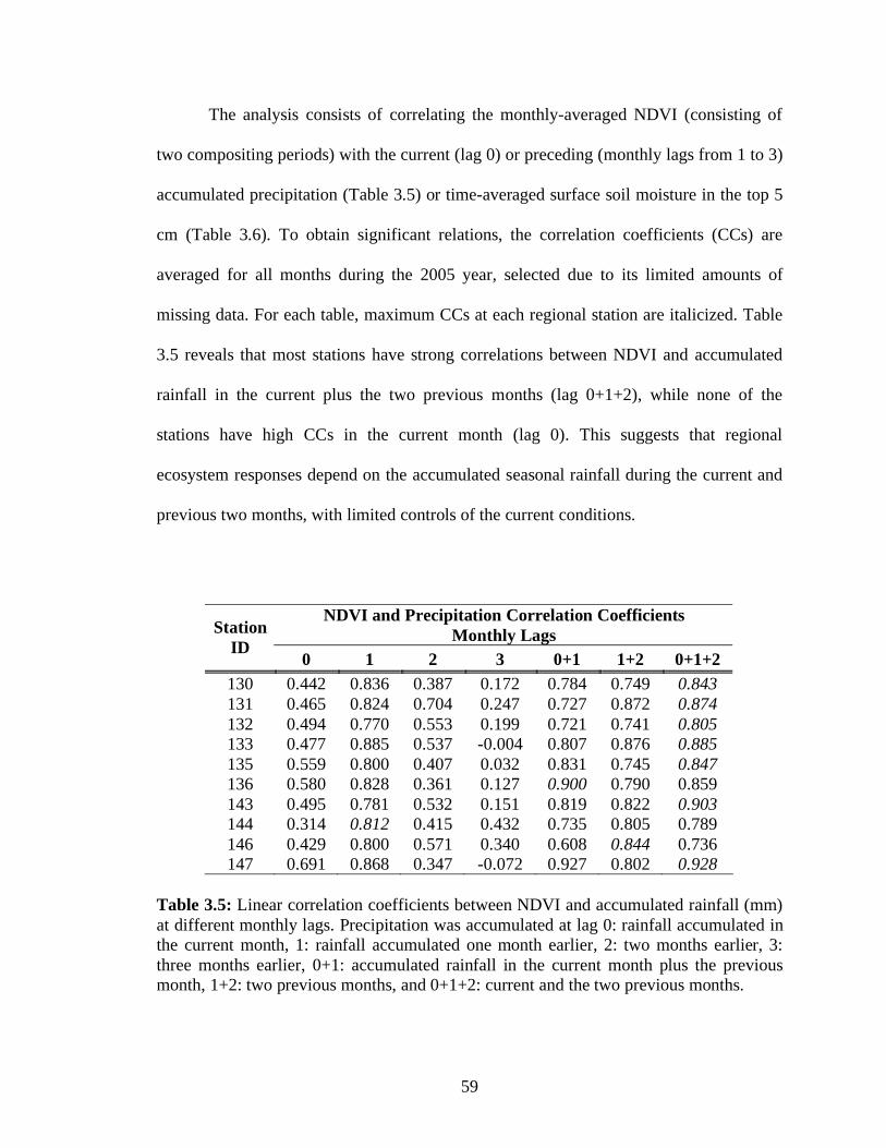
59

The analysis consists of correlating the monthly-averaged NDVI (consisting of

two compositing periods) with the current (lag 0) or preceding (monthly lags from 1 to 3)

accumulated precipitation (Table 3.5) or time-averaged surface soil moisture in the top 5

cm (Table 3.6). To obtain significant relations, the correlation coefficients (CCs) are

averaged for all months during the 2005 year, selected due to its limited amounts of

missing data. For each table, maximum CCs at each regional station are italicized. Table

3.5 reveals that most stations have strong correlations between NDVI and accumulated

rainfall in the current plus the two previous months (lag 0+1+2), while none of the

stations have high CCs in the current month (lag 0). This suggests that regional

ecosystem responses depend on the accumulated seasonal rainfall during the current and

previous two months, with limited controls of the current conditions.

NDVI and Precipitation Correlation Coefficients

Monthly Lags Station

ID 0 1 2 3 0+1 1+2 0+1+2

130 0.442 0.836 0.387 0.172 0.784 0.749 0.843

131 0.465 0.824 0.704 0.247 0.727 0.872 0.874

132 0.494 0.770 0.553 0.199 0.721 0.741 0.805

133 0.477 0.885 0.537 -0.004 0.807 0.876 0.885

135 0.559 0.800 0.407 0.032 0.831 0.745 0.847

136 0.580 0.828 0.361 0.127 0.900 0.790 0.859 143 0.495 0.781 0.532 0.151 0.819 0.822 0.903

144 0.314 0.812 0.415 0.432 0.735 0.805 0.789 146 0.429 0.800 0.571 0.340 0.608 0.844 0.736 147 0.691 0.868 0.347 -0.072 0.927 0.802 0.928

Table 3.5: Linear correlation coefficients between NDVI and accumulated rainfall (mm) at different monthly lags. Precipitation was accumulated at lag 0: rainfall accumulated in the current month, 1: rainfall accumulated one month earlier, 2: two months earlier, 3: three months earlier, 0+1: accumulated rainfall in the current month plus the previous month, 1+2: two previous months, and 0+1+2: current and the two previous months.

60

Conversely, the correlation coefficients between monthly NDVI and time-

averaged soil moisture in Table 3.6 exhibit larger values for the current (lag 0), previous

(lag 1) or current and previous (lag 0+1) months. The shorter monthly lags observed for

the maximum CCs between NDVI and soil moisture are evidence of a more immediate

control of plant available water on vegetation dynamics, as compared to current

precipitation. Nevertheless, overall CCs between NDVI and precipitation are higher than

those for soil moisture at longer monthly lags across most of the regional stations. Fig.

3.4 summarizes the differences between the precipitation and soil moisture correlations

with NDVI for a range of lags arranged from the current month (lag 0) toward longer

prior periods (lag 0+1+2). Results are shown as average values (symbols) over all

stations and their variability depicted as the ±1 standard deviation (vertical bars). Clearly,

the concurrent correlation (lag 0) is higher between soil moisture and NDVI, as compared

with the current precipitation amount. For longer lags (e.g., lag 0+1, 0+1+2), however,

the accumulated rainfall has a stronger relation with the vegetation dynamics, indicating

that the delayed response between NAM rainfall and seasonal greening in the region. It is

important to clarify that we used superficial soil moisture (5 cm depth) and one concern

is if this depth is representative of the entire root profile. In order to demonstrate if the

surface soil moisture is representative of the root soil moisture profile, we performed a

correlation matrix for station 147. The dataset includes soil moisture readings at 5, 10 and

15 cm from the period 2004-2006 (not shown here). We found that surface soil moisture

is well correlated with deeper soil moisture values (see Figure 3.5).

61

Figure 3.4: Linear correlation coefficients (CCs) between monthly NDVI and accumulated precipitation and averaged soil moisture over a range of different monthly lags, arranged from current (lag 0) toward longer prior periods (lag 0+1+2). CCs are shown as averages (symbols) and standard deviations (±1 std as vertical bars) over all stations in 2005.

NDVI and Soil Moisture Correlation Coefficients

Monthly Lags Station

ID 0 1 2 3 0+1 1+2 0+1+2

130 0.450 0.706 0.344 0.080 0.675 0.612 0.700 131 0.406 0.828 0.631 0.153 0.672 0.818 0.803 132 0.435 0.627 0.557 0.381 0.572 0.631 0.616 133 0.673 0.720 0.274 -0.200 0.781 0.584 0.752 135 0.582 0.381 -0.174 -0.421 0.537 0.120 0.347 136 0.548 0.454 0.093 -0.040 0.554 0.381 0.528 143 0.683 0.778 0.381 -0.008 0.877 0.677 0.881

144 0.572 0.766 0.351 0.154 0.769 0.635 0.754 146 0.542 0.790 0.505 0.229 0.717 0.765 0.819

147 0.589 0.655 0.293 -0.063 0.684 0.541 0.629

Table 3.6: Linear correlation coefficients between NDVI and averaged surface soil moisture at different monthly lags. Soil moisture was averaged over lag 0: current month, 1: one month earlier, 2: two months earlier, 3: three months earlier, 0+1: current month plus the previous month, 1+2: two previous months, and 0+1+2: current plus the two previous months

62

Station 147

DOY

290 295 300 305 310 315 320 325 330 335 340 345 350 355 360

Sil M

it

(%)

0

5

10

15

20

25

30

3.5 to 6.5 cm

Profile ( 3.5 to 16.5 cm)

Figure 3.5: Comparison between surface soil moisture and root zone profile at station 147 (Rayon tower). Dots represent mean daily values and the bars ±1 standard deviation.

This is in agreement with several authors (Martinez et al, 2008; Mahmood et al,

2007; Calvet et al 1998, Grayson and Western, 1998) who found that surface soil

moisture is well correlated with root zone soil moisture (0-30 cm). However, the

correlation declines fast at deeper soil layers. Furthermore, according to Hillel (1971), the

upper dry surface layer in sandy soils (most of the soils in the region are sandy-loam)

forms, during soil drying, a type of barrier that restricts the evaporation of soil water only

to this dry surface layer (DSL). Therefore, the soil moisture is well distributed below this

DSL. In addition, Barnes and Allison (1983) explained that water moves upward in the

liquid phase in the zone below the DSL, hence; water is transported by vapor diffusion in

the zone above the DSL.

63

In addition, we observed that in wet periods the variability in the profile is high

and decreases with soil drying. Therefore it is more reliable to compare the surface and

root zone soil moisture in dry rather than wet periods. This is in agreement with authors

that reported that variability in soil profile increases with increase in soil moisture content

(Martinez et al, 2008; Famiglietti et al, 1998; Mohanty et al 2008; De Lannoy et al,

2006). Hence, surface soil moisture is a good predictor of root zone status; however, it is

more accurate if we compare both values during drying periods. For the shallow rooted

plants in regional ecosystems, the surface moisture determines plant water uptake and

evapotranspiration (Casper et al., 2003; Seyfried and Wilcox, 2006; Vivoni et al. 2008).

3.4. Spatial and Temporal Stability Analyses of Vegetation Dynamics

3.4.1 Spatial and Temporal Stability of NDVI

The ecosystem response to precipitation and soil moisture conditions, as captured

by the NDVI fields, can be discerned through spatial and temporal persistence. Fig. 3.6

presents spatial maps of: (a) the spatial RMSE s, and (b) the temporal RMSE t,

calculated using the eighty-three (83) MODIS NDVI images in the domain. Regions with

low spatial RMSE s (Fig. 3.6a, red colors) correspond to zones that closely track the

spatially-averaged conditions in the two basins. These areas coincide well with the

location of Sinaloan thornscrub and Sonoran desert scrub (Brown, 1994) that exhibit

strong seasonal variations in NDVI and occupy large regional extents. Note these areas

are located over a range of elevations, but are not observed in the highest peaks or

riparian corridors (Vivoni et al., 2007).

64

Figure 3.6: Spatial distributions of spatial and temporal RMSE for: (a, b) NDVI, (c, d) Albedo and (e, f) LST. Resolution for NDVI is 250-m, while albedo and LST are 1-km.

65

In these locations, high spatial RMSE s (Fig. 3.6a, blue colors) indicate zones

behaving differently from the spatial mean and correspond to Madrean evergreen

woodland and montane conifer forests at high elevations and Sonoran riparian deciduous

woodland along the main stems of the Río San Miguel and Río Sonora. Clearly, the

distribution of RMSE s is a useful tool to classify ecosystem patterns, in particular to

sharply distinguish between evergreen woodlands at high elevations and deciduous

scrublands at mid elevations.

The temporal RMSE t (Fig. 3.6b) supports the above analysis by distinguishing

locations in the domain that closely track the temporal mean in each pixel. Regions with

low RMSE t (blue colors) have relatively smaller changes in time and correspond to

Madrean evergreen woodland and montane conifer forests at high elevations and Sonoran

riparian deciduous woodlands along rivers. Despite having deciduous trees, the riparian

woodlands are able to directly access groundwater and thus remain green during longer

periods of time, as compared to ecosystems that rely solely on summer rainfall. Lower

temporal persistence is observed for regions with high RMSE t (red colors) which depict

zones with large temporal changes. Clearly, these match the areas with low RMSE s, in

particular the Sinaloan thornscrub and Sonoran desert scrub. Interestingly, the temporal

RMSE t is able to more clearly separate the locations of these ecosystems, with Sinaloan

thornscrub further south in the domain and replaced by Sonoran desert scrub at similar

elevations in the north (Brown, 1994). In conjunction, the spatial and temporal

persistence maps reveal ecosystem patterns that are not observed through simpler metrics

such as seasonal NDVI changes (Fig. 3.1). Further, this analysis extends applications of

RMSE beyond traditional soil moisture studies (e.g., Jacobs et al., 2004; Vivoni et al.,

66

2008a). Recognition of these patterns is important because we can identify zones with

dramatic changes in vegetation dynamics that can affect the ecosystem energy balance.

As result, we expect to find vegetation-rainfall feedback regions where greater changes in

the energy balance are observed, helping to generate more convective rainfall.

3.4.2 Spatial and Temporal Stability of Albedo

Fig. 3.6 also presents the RMSE metrics for albedo and LST at a coarser

resolution (1-km). Correspondence between the spatial RMSE for albedo and NDVI

indicates that albedo changes are primarily due to vegetation greening. Regions with low

spatial persistence in albedo include grasslands located in the northern part of the study

region and semidesert shrublands found in the coastal plains, which do not track the

spatial mean of the region (Fig. 3.6c). In addition, these ecosystems also showed low

variability in time (very low seasonality). High elevation sites, as well as some riparian

corridors had a moderately spatial representativeness of the region. Conversely,

subtropical scrublands represent the spatial mean well and have moderate seasonality

linked to their dynamic NDVI changes (Fig. 3.6d). In the other hand, high elevations

showed high variability in time. Because albedo is highly affected by soil moisture status

and high elevation ecosystems tend to receive more rainfall than the rest of the biomes in

the region, therefore we expect more fluctuations in albedo values. Since the temporal

RMSE in albedo has a heterogeneous pattern with a low range, this indicates a local

control by soil and vegetation conditions on its moderate temporal changes.

67

3.4.3. Spatial and Temporal Stability of Land Surface Temperature

LST exhibits spatial RMSE (Fig. 3.6e) that resembles the NDVI pattern

suggesting that surface temperature variations are closely tied to vegetation dynamics.

Differences, however, are observed between the temporal RMSE of LST (Fig. 3.6f) and

NDVI. A clear gradient in LST RMSE from high to low variability occurs from the

northwest to the southwest corners of the region. This can be attributed to larger LST

variations in mountain regions, as compared to more consisted high temperatures in

desert areas. The differences in surface temperature variability reflects very well the

climatic differences along the state of Sonora with the less variability found in the coastal

plains (desert scrub, with smaller range of temperature differences during seasons) and

higher variability when we approach the mountain ranges to the east (larger range of

temperature during seasons). Also, there is a latitudinal effect observed in the variability

of land surface temperature. Variability increases from southern to northern latitudes

where snow is present and we can find a wider range of temperatures between seasons.

3.5. Topographic Control on Vegetation Dynamics

Given the observed effects of topography on spatial and temporal persistence, it is

important to understand how ecosystem responses vary along elevation gradients in the

study region. Figs. 3.7 and 3.8 present the variation of NDVI, spatial RMSE s and

temporal RMSE t for two topographic transects depicted in Fig. 2.1 (A A’ in the Río

San Miguel and B B’ in the Río Sonora). The transects were selected to capture a range

of elevations (550 to 1900 m in A A’, and 680 to 1600 m in B B’), span several

ecosystems and be in proximity to a subset of the regional stations. Note that Figs. 3.7

68

and 3.8 indicate the topographic variations (solid lines) with distance along the transects,

which have a total planform length of ~23 km. In both topographic transects, the

temporal mean NDVI (symbols) increases with elevation, while the temporal standard

deviation (vertical bars depict ±1 std) typically decreases with altitude. These variations

indicate that the mid elevation Sinaloan thornscrub and Sonoran desert scrub are

characterized by lower time-averaged greenness, which is more variable in time, as

compared to the high elevation Madrean evergreen woodland. Notably, the Río San

Miguel transect exhibits higher NDVI (> 0.70) in the mountain peak (up to 1900 m) than

the Río Sonora peak (NDVI > 0.55). Interestingly, the relation between NDVI and

elevation at lower and mid elevations (e.g., ~600 to 1000 m for Río San Miguel) is linear,

with similar rates of increase along the transect. At high elevations, however, a lag is

observed in the increase in NDVI as compared to elevation as well as a displacement of

the NDVI maximum value away from the peak elevation.

The relation between elevation and ecosystem response is further analyzed using

the spatial and temporal persistence in Fig. 3.7b and 3.8b. In both transects, the mid

elevation ecosystems exhibit low spatial RMSE s and high temporal RMSE t, which

indicate areas closely tracking the mean conditions in the region. These elevations

correspond to Sinaloan thornscrub and Sonoran desert scrub which are highly responsive

to NAM precipitation and occupy large regional extents. At high elevations along each

transect, the Madrean evergreen woodland has a larger spatial RMSE s and a smaller

temporal RMSE t. This suggests that the evergreen species have time-stable conditions

that do not track the spatially-averaged response. In addition, the maximum spatial

RMSE s is displaced slightly from the mountain peak, as observed for the mean NDVI.

69

Figure 3.7: Topographic control on vegetation metrics in the Río San Miguel transect. (a) Relation between elevation and temporal mean NDVI (closed circles) and the temporal standard deviation (±1 std as vertical bars). (b) Relation between elevation and spatial and temporal RMSE .

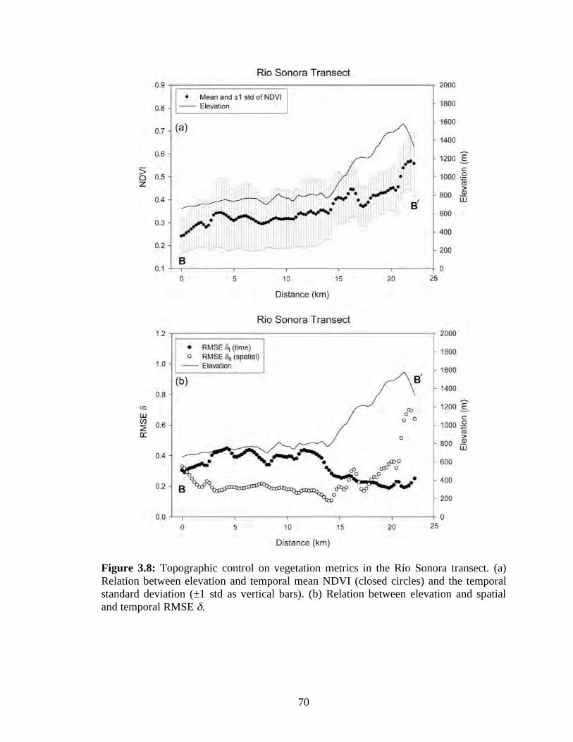
70

Figure 3.8: Topographic control on vegetation metrics in the Río Sonora transect. (a) Relation between elevation and temporal mean NDVI (closed circles) and the temporal standard deviation (±1 std as vertical bars). (b) Relation between elevation and spatial and temporal RMSE .

71

In both transects, a range of elevations (e.g., ~600 to 900 m in the Río San

Miguel) simultaneously have small spatial and temporal RMSE . We interpret this as an

elevation band of significant monsoonal response, which dominates the regional

greening, as suggested by Vivoni et al. (2007).

Clearly, spatial and temporal persistence reveal variations in vegetation dynamics

along topographic transects and can aid in the interpretation of vegetation-elevation

relations in semiarid mountain fronts. Because both transects in San Miguel and Sonora

Basins give similar results we will focus only in San Miguel basin transect for the

analysis of albedo and land surface temperature. Figure 3.9a shows the topographic

controls on mean value of albedo for the San Miguel transect for the period 2004-2007.

We can clearly see that albedo is decreasing with increase in elevation along the transect.

Conversely, we observe that albedo variability (expressed as error bars with the value of

standard deviation) increases as elevation increases. It is important to mention that

variability as well as mean albedo showed an inflection point around 1200 m above sea

level. As we argue in the previous section, we believe that high elevation leads to more

precipitation and, in consequence, higher surface soil moisture as well as vegetation

cover. These two conditions highly affects albedo, therefore we expect more variability in

albedo in higher elevation ecosystems such as Madrean evergreen forest. Figure 3.9b

shows the behavior of the spatial and temporal RMSE . Spatial RMSE as well as

temporal RMSE increases with elevation. Hence, higher elevation sites moderately

represent the regional mean and moderately deviate from the temporal mean of the

region, showing slightly higher seasonality than lower elevation ecosystems.

72

Figure 3.9: Topographic control on albedo in the Río San Miguel. (a) Relation between elevation and temporal mean albedo (closed circles) and the temporal standard deviation (±1 std as vertical bars). (b) Relation between elevation and spatial and temporal RMSE .

73

Figure 3.10: Topographic control on land surface temperature in the Río San Miguel. (a) Relation between elevation and temporal mean albedo (closed circles) and the temporal standard deviation (±1 std as vertical bars). (b) Relation between elevation and spatial and temporal RMSE .

74

Figure 3.10a shows the topographic control on mean Land Surface Temperature

(LST). As we expected, surface temperature decreases with elevation. How ever, there is

a slightly decrease in variability for LST with elevation. Again, elevation is playing an

important role in the decrease of surface temperature. Higher elevation leads to more

precipitation; hence, increasing the soil moisture at the soil surface and plant greening.

Water released from the soil and plant leaves (as evaporation and transpiration) produces

a cooling effect on the surface and air temperatures. Finally, we observed a slightly

decrease in temporal RMSE with elevation (seasonality). At least in this region,

temperature does not change as much as shown in Figure 3.6, where larger LST

variability is observed in the northern latitudes and in higher elevation in the Sierra

Madre Occidental. Figure 3.10b shows the distribution of spatial RMSE s increases with

elevation, suggesting that higher elevation ecosystems did not track the spatial mean of

the region, unlike lower elevation ecosystem, such as the Sinaloan thornscrub. We

calculated a lapse rate for the San Miguel Basin of 14 °C/km which is more than double

of the atmospheric lapse rate (6.5 °C/km). The difference is caused by thermal properties

of both materials where soil has higher thermal conductivity than air (2.4 W/mK

compared to 0.025 W/mK respectively).

3.6. Identifying Land Surface Response Functional Groups

Fig. 3.11 presents the characteristics of six functional groups (FG) derived from

the cluster analysis and unsupervised classification of the spatial and temporal persistence

of NDVI, albedo and LST. FGs represent zones that have similar land surface responses

to precipitation and solar radiation forcing. Their spatial distribution (Fig. 3.11a)

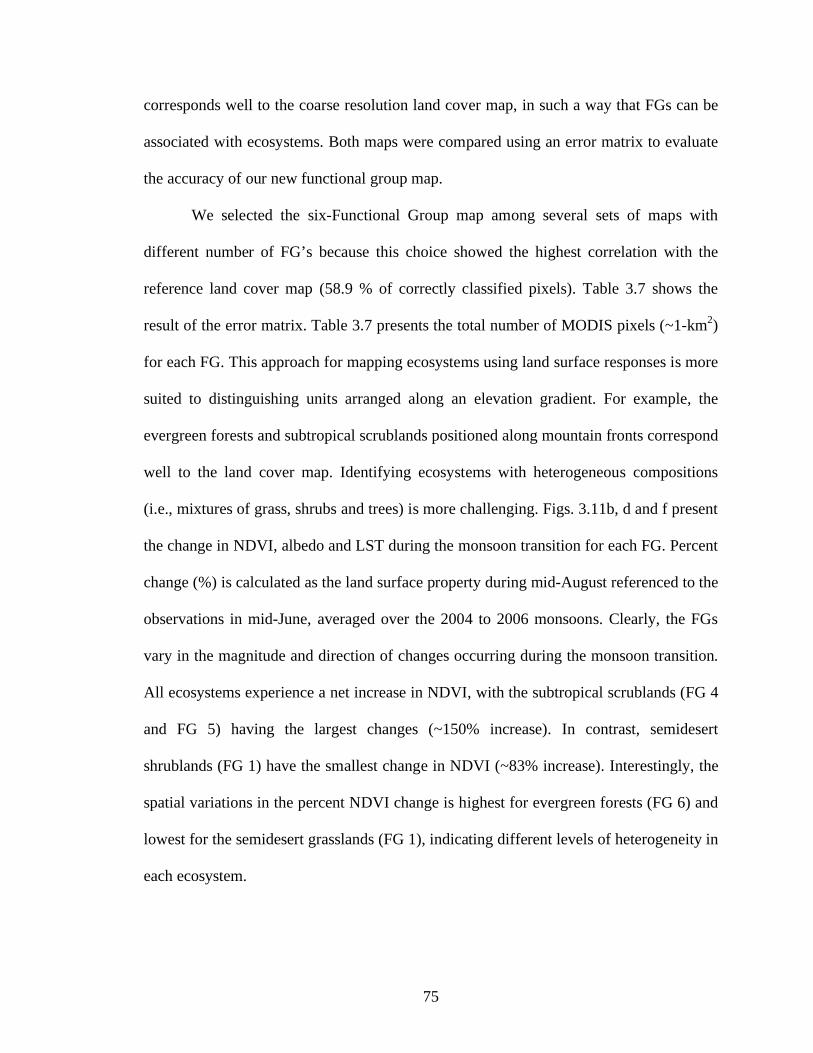
75

corresponds well to the coarse resolution land cover map, in such a way that FGs can be

associated with ecosystems. Both maps were compared using an error matrix to evaluate

the accuracy of our new functional group map.

We selected the six-Functional Group map among several sets of maps with

different number of FG’s because this choice showed the highest correlation with the

reference land cover map (58.9 % of correctly classified pixels). Table 3.7 shows the

result of the error matrix. Table 3.7 presents the total number of MODIS pixels (~1-km2)

for each FG. This approach for mapping ecosystems using land surface responses is more

suited to distinguishing units arranged along an elevation gradient. For example, the

evergreen forests and subtropical scrublands positioned along mountain fronts correspond

well to the land cover map. Identifying ecosystems with heterogeneous compositions

(i.e., mixtures of grass, shrubs and trees) is more challenging. Figs. 3.11b, d and f present

the change in NDVI, albedo and LST during the monsoon transition for each FG. Percent

change (%) is calculated as the land surface property during mid-August referenced to the

observations in mid-June, averaged over the 2004 to 2006 monsoons. Clearly, the FGs

vary in the magnitude and direction of changes occurring during the monsoon transition.

All ecosystems experience a net increase in NDVI, with the subtropical scrublands (FG 4

and FG 5) having the largest changes (~150% increase). In contrast, semidesert

shrublands (FG 1) have the smallest change in NDVI (~83% increase). Interestingly, the

spatial variations in the percent NDVI change is highest for evergreen forests (FG 6) and

lowest for the semidesert grasslands (FG 1), indicating different levels of heterogeneity in

each ecosystem.

76

Class

Semidesert shrubland

Semidesert grassland

Mixed shrubland

Subtropical scrubland (low

elevation)

Subtropical scrubland (high

elevation)

Madrean evergreen woodland Totals

1 291 78 35 97 66 309 876

2 268 510 103 964 21 46 1912

3 95 25 275 502 31 92 1020

4 85 208 127 1012 15 35 1482

5 27 206 431 277 117 23 1081

6 2 251 143 44 6 4336 4782

Totals 768 1278 1114 2896 256 4841 11153

Correct pixels: 6541 Percentage of correct pixels: 58.6 %

Table 3.7: Error matrix showing the comparison between the new functional groups map and a reference map (Land cover map generated by Yilmaz et al. (2008)). The classes shown horizontally represent the classes of the reference map; conversely, the classes shown vertically represent the classes in the generated map. The number of pixels shaded and shown diagonally represents the number of correctly classified pixels by category.

The monsoon transition in albedo has a strong dependence on the functional

group. Low elevation FGs (1 to 3) exhibit a decrease in albedo, on average, while the

high elevation FG 6 has an increase in albedo during the monsoon (Fig. 3.11d). This

contrast is likely due to the dual roles of soil color and vegetation greenness on

determining albedo (Sandholtz et al., 2002). In addition, large spatial variations occur in

each FG due to the heterogeneous nature of the albedo response. LST exhibits a general

decrease in all FGs, with a lower reduction for semidesert shrublands (FG 1). Other FGs

exhibit decreases in LST from 3 to 5% and moderate spatial variations. This is due to a

widespread effect of soil moisture, through evapotranspiration, on reducing surface

temperatures during the monsoon transition. Comparing across the NDVI, albedo and

LST changes, the subtropical scrublands (FG 4 and 5) show the largest increases in

NDVI, large decreases in LST, and a decrease, on average, in albedo.

77

Figure 3.11: (a) Land surface response functional groups obtained from cluster analysis. Mean spatial percent change during NAM for each functional group for: (b) NDVI, (d) Albedo and (f) LST. Error bars represent ± 1 spatial standard deviation. Relation between mean spatial and temporal RMSE by functional group for: (c) NDVI, (e) Albedo and (g) LST. Functional groups are ordered with increasing elevation (see legend for functional group name).

Table 3.8 summarizes the overall behavior for all functional groups and the

corresponding percentage of total area for each FG. Figs. 3.11c, e and g present the

spatial and temporal RMSE averaged for each FG and its spatial variability. As

discussed previously, FGs with low spatial RMSE represent well the regional mean,

while FGs with low temporal RMSE exhibit low seasonality. We highlight the response

in subtropical scrublands (FG 4 and FG 5) since this ecosystem is monitored at an eddy

covariance tower site.

78

Functional

Group Ecosystem Classification

Number of

Pixels

(Percent

Area)

Direction of Change in

Monsoon

NDVI Albedo LST

1 Semidesert shrubland 5213 (8.8%) + - -

2 Semidesert grassland 10290 (17.4%) + - -

3 Mixed shrubland 8675 (14.6%) + - -

4 Subtropical scrubland (low elevation) 15518 (26.2%) + ± -

5 Subtropical scrubland (high elevation) 9112 (15.4%) + - -

6 Madrean evergreen woodland 10450 (17.6%) + + -

Table 3.8: Functional group characteristics, including the direction of change in the spatially-average land surface property (NDVI, albedo, LST) during the monsoon transition: increase (+), decrease (-) and no net change (±). See Fig. 3 for the spatial variability. The number of pixels refers to the MODIS pixel resolution (~1 km2), in parenthesis is the percent of the total area.

The large areas occupied by subtropical scrublands (~21,150 km2) have high

seasonality in NDVI and LST; and dominate the regional response in NDVI, albedo and

LST. As a result, the tower site is representative of the land surface conditions in a broad

region that responds vigorously to the NAM. The high representativeness extent of the

tower site in subtropical scrublands fills a major observational gap in the Sonoran Desert

(Yang et al., 2008).

3.7. Vegetation-Rainfall Feedback Mechanism in Subtropical Scrubland

Fig. 3.12 presents the land surface transitions at the eddy covariance tower during

the 2007 monsoon. The monsoon onset, indicated by the precipitation pulses, occurred

79

near Julian day 185 (July 4, 2007). Precipitation (P) led to high soil moisture in the

surface layer, which increased from ~2% to 10%. Vegetation responded quickly to soil

water, increasing from NDVI = 0.20 to 0.55. Vegetation greenup led to a decrease in

albedo, consistent with estimates from MODIS. In addition, soil temperature decreased

from ~43 to 37 °C, which matched with the MODIS LST. Lower LST is a result of the

cooling effects of evapotranspiration, as shown by the decreasing Bowen ratio.

The Bowen ratio (B) is the ratio of sensible to latent heat flux. Field data indicate

a positive relation between NDVI and P, and a negative relation between LST and P.

According to Brunsell (2006), these correlations indicate a positive vegetation-rainfall

feedback, but do not imply direct causality. As a result, a close inspection of the tower

data can help infer the sign and pathways of the feedback in the subtropical scrubland.

Observed transitions are summarized in Table 3.9 by comparing the pre-monsoon and

monsoon-averaged values. Fig. 3.12c illustrates a theoretical pathway through which

positive anomalies in soil moisture and vegetation greening lead to more rainfall, adapted

from Eltahir (1998). We test whether the positive vegetation-rainfall feedback holds

based on the observations. The thick boxes indicate the data that supports Eltahir (1998),

including: (a) an increase in vegetation greenness, (b) a decrease in albedo, (c) a decrease

in B, (d) an increase in water vapor in the boundary layer, (e) a decrease in LST, and (f)

an increase in net terrestrial radiation. The field data, however, do not support an increase

in the net solar radiation (thick dashed box). In fact, a strong decrease occurs in net solar

radiation (Table 3.9), primarily due to cloudiness.

80

Figure 3.12: (a) Transition in NDVI, albedo, Bowen ratio and precipitation during the 2007 monsoon season. (b) Transition of soil temperature, net radiation, soil moisture and precipitation. Gaps in net radiation correspond to cloudy days not included in analysis. (c) Diagram relating changes in soil moisture and vegetation greenness with the subsequent effects in land-atmosphere interactions and rainfall, adapted from Eltahir (1998).

We capture this negative interaction by the dashed line linking the convective

storms to net solar radiation. Overall, this negative interaction suppresses the increase in

net terrestrial radiation and promotes only a small change in net radiation. For dry

monsoon days, net radiation averages 13.35 MJ/day (N = 17), while for wet days it is

14.86 MJ/day (N = 33). This indicates that for days with wet soils, we observe a slight

increase in net radiation relevant to the pre-monsoon period (13.98 MJ/day).

81

Table 3.9: Comparison of ground-based and remotely-sensed variables tower. Before monsoon has 34 days: DOY 151 (May 31, 2007) to DOY 184 (July 3, 2007). During monsoon period has 56 days: DOY 185 (July 3, 2007) to DOY 240 (August 28, 2007).

How do we reconcile the observed trends in the monsoon transition with the

proposed vegetation-rainfall feedback? As noted by Brunsell (2006), there is an important

distinction between vegetation effects on the surface energy balance that enhance

precipitation and those that suppress it. From this evidence, we infer that a positive

vegetation-rainfall feedback exists only when the effects of clouds do not decrease net

solar radiation. This would occur, for example, on sunny days following a precipitation

pulse. Julian days 201-202 (July 19 to 20, 2007) demonstrate this sequence (Table 3.10).

In this two-day period, land surface conditions can promote subsequent rainfall.

Persistent cloudy conditions can weaken the vegetation-rainfall feedback. For example,

Julian days 215-216 (August 3 to 4, 2007) have sufficient cloudiness to decrease net

radiation, interrupting the proposed pathway, despite having the other elements (Table

3.10). This comparison suggests that the negative interaction relating cloudiness to net

solar radiation is important for the vegetation-rainfall feedback. This feedback

Data Source Land Surface Variable and Unit Pre-Monsoon Monsoon

Tower Rainfall (mm) 8.64 227.58 Albedo (-) 0.17 0.15 Bowen Ratio (-) 13.27 1.84 Net Radiation (MJ/day) 13.98 13.70 Net Solar Radiation (MJ/day) 25.82 18.62 Net Terrestrial Radiation (MJ/day) -11.77 -4.92 Soil Moisture (%) 2.36 7.43 Soil Temperature (˚C) 43.11 36.84 Vapor Pressure (mb) 1.06 2.22 MODIS Albedo (-) 0.17 0.14 NDVI (-) 0.20 0.56 LST (˚C) 39 30

82

mechanism operates at seasonally scale because the feedback mechanism proposed by

Eltahir (1998) is based in two basic properties of the land surface that we have monitored

in this thesis: 1) the albedo and 2) the Bowen ratio. The changes in these two variables

occur at seasonal scale (three or four months). The transition between dry and wet

conditions occurs rapidly, but the temporal persistence of these land surface properties

stay for several months.

Table 3.10: Comparison of changes in ground observations during two-day sequences exhibiting a positive vegetation-rainfall feedback (Day 1 and 2 = Julian days 201 and 202); and a weakened feedback due to the effects of cloudiness (Day 1 and 2 = Julian days 215 and 216).

Vegetation-Rainfall

Feedback Land Surface Variable and Unit Day 1 Day 2

Positive feedback Precipitation (mm/day) 6.10 11.68 Julian day 201 to 202 Albedo (-) 0.152 0.149 Bowen Ratio (-) 4.97 0.75 Net Radiation (MJ/day) 11.98 15.42 Net Solar Radiation (MJ/day) 15.49 19.60 Net Terrestrial Radiation (MJ/day) -3.51 -4.17 Soil Moisture (%) 3.85 7.75 Soil Temperature (˚C) 39.2 34.3 Vapor Pressure (mb) 2.12 2.28

Weakened Feedback Precipitation (mm/day) 0.76 17.53 Julian day 215 to 216 Albedo (-) 0.161 0.153 Bowen Ratio (-) 0.83 0.08 Net Radiation (MJ/day) 6.43 4.04 Net Solar Radiation (MJ/day) 8.80 5.08 Net Terrestrial Radiation (MJ/day) -2.37 -1.04 Soil Moisture (%) 7.18 7.76 Soil Temperature (˚C) 36.9 30.2 Vapor Pressure (mb) 2.37 2.53

83

CHAPTER 4

CONCLUSIONS AND FUTURE WORK

Vegetation dynamics in the North American monsoon region are closely linked to

seasonal changes in precipitation (e.g., Salinas-Zavala et al., 2002; Matsui et al., 2005;

Watts et al., 2007; Vivoni et al., 2007). To the authors’ knowledge, however, the controls

exerted by precipitation and soil moisture on seasonal vegetation greening have not been

studied for the broader NAM region in northwest Mexico. Furthermore, the seasonal,

interannual and spatial variations in vegetation response during the NAM are not well

understood. Quantifying these spatiotemporal variations in a range of ecosystems is

fundamental for assessing the degree of coupling between ecologic, hydrologic and

atmospheric processes during the summer season. For example, Dominguez et al. (2008)

found that the dynamics of evapotranspiration in the NAM ecosystems leads to a positive

feedback on rainfall generation and to local precipitation recycling. Since the

spatiotemporal variations of vegetation greening are directly linked to photosynthesis and

evapotranspiration, quantifying vegetation dynamics using remote sensing observations

represents an important step towards investigating ecohydrological processes in the NAM

region. While vegetation greening should clearly be related to precipitation and soil

moisture in the water-limited ecosystems, no prior attempts have been made to quantify

the hydrologic controls on the vegetation dynamics. Also, it is important to evaluate land

surface changes to understand their potential role in the precipitation processes during the

NAM (e.g., Dominguez et al., 2008; Vivoni et al., 2008b).

84

In this thesis, we quantify the seasonal and interannual changes in vegetation

greenness through the use of remotely-sensed vegetation index fields from the MODIS

sensor over the period 2004 to 2006. We present the changes in land surface conditions

occurring during the NAM though the combined use of remote sensing observations and

ground-based data. Our regional analysis focuses on a large area in northern Sonora

comprised by two major basins (Río San Miguel and Río Sonora) and parts of the Río

Yaqui and San Pedro River basins in the Sierra Madre Occidental. The regional extent

and the study duration were selected to take advantage of the regional instrument network

with precipitation and soil moisture observations. By relating and interpreting the

remotely-sensed and ground-based measurements, we identify the following

characteristics of the regional vegetation dynamics in the Sierra Madre Occidental of

northern Sonora and their relation to precipitation and soil moisture:

(1) Seasonal changes in vegetation greenness are dramatic in all the regional

ecosystems and are related to hydrologic conditions and their spatial distribution during a

particular monsoon season. As a result, interannual variability is observed in the seasonal

vegetation greening and the metrics used to quantify biomass production. The vegetation

response was most intense and extensive during the wet 2006 monsoon, reaching up to a

300% seasonal increase in NDVI.

(2) Vegetation responses to NAM precipitation and soil moisture depend strongly

on the plant communities in each ecosystem. The ecosystem with consistently high

monsoon greening is the mid elevation Sinaloan thornscrub, as suggested by Watts et al.

(2007) and Vivoni et al. (2007). Other ecosystems in the region either exhibited lower

seasonal changes in NDVI or less consistent year-to-year variations. Comparisons across

85

ecosystems indicate that different plant greenup strategies are utilized in response to

interannual hydrologic variations.

(3) Spatial and temporal persistence of remotely-sensed NDVI fields reveal

ecosystem patterns that are not observed using simple metrics. In particular, RMSE s

distinguishes between evergreen woodlands at high elevations and deciduous scrublands

at mid elevations, while the temporal RMSE t can more clearly separate different

ecosystems at similar elevations. Analysis along two topographic transects indicate that

elevation controls vegetation dynamics and serves to organize ecosystems into elevation

bands, with high monsoonal response at mid elevations.

(4) Accumulated seasonal precipitation is a strong indicator of biomass

production across the regional ecosystems, with Sinaloan thornscrub exhibiting the

highest rainfall use efficiency. During the study period, differences between ecosystem

responses were minimized during the wet 2006 monsoon and maximized during drier

monsoons, in contrast to the common rainfall use efficiency found by Huxman et al.

(2004) during drought years. Additional studies are required to quantify rainfall use

efficiency in wet and dry periods in the regional ecosystems.

(5) Lagged correlation analysis indicates a strong degree of coupling between

vegetation greening and the precipitation and soil moisture conditions at each regional

station. Interestingly, concurrent correlations for monthly NDVI are higher with surface

soil moisture, while lagged correlations are more significant for accumulated

precipitation. This suggests that soil moisture plays an important intermediary role

between NAM precipitation and vegetation response.

86

In addition, with the help of remote sensing observations, we identify areas

exhibiting the potential for a vegetation-rainfall feedback, and then with the use of

ground-based observations, we identify the sign, pathways, and interruptions in the

feedback mechanism. From this analysis, we can also conclude:

(6) The spatial and temporal persistence of NDVI, albedo and LST identifies

areas with strong seasonality that represents the regionally-averaged dynamics. Changes

in land surface conditions for the areally-extensive subtropical scrublands exhibit the

necessary trends in NDVI, albedo and LST for a positive vegetation-rainfall feedback.

(7) Observations at an eddy covariance tower site in the subtropical scrubland

indicate that the necessary trends in land surface variables are exhibited for a positive

vegetation-rainfall feedback if persistent cloudiness does not occur. The effects of clouds

on net solar radiation can weaken or interrupt the positive feedback mechanism.

The observational analysis and interpretations conducted here show the

importance of combining satellite remote sensing and ground networks for monitoring

ecosystem dynamics and their link to hydrologic conditions. The use of multiple

observation scales allows understanding the regional context in which detailed

precipitation, soil moisture or surface flux measurements have been made (Gebremichael

et al., 2007; Vivoni et al., 2007; Watts et al., 2007). In particular, it is clear that

substantial interannual variations are present in monsoon vegetation greening. Clearly,

the duration of our study is a limitation in our interannual analysis, primarily due to the

recent establishment of the regional network. Additional analysis is desirable either by

extending the work as new data sets become available or performing retrospective

analysis with satellite data (though ground data would be limited).

87

Several additional questions have arisen through the analysis conducted in this

thesis. While our focus has been on the summer season, the response to lower and more

variable winter precipitation appears to be significant, in particular for Sonoran savanna

grasslands during wet winters. The other regional ecosystems also appear to maintain

greener conditions for longer periods when winter rainfall is available. Spring season

growth is more common in higher latitude desert grasses (e.g., Pennington and Collins,

2007). As a result, the influence of winter precipitation on the annual hydrologic cycle

and vegetation dynamics warrants further study.

The linkages between winter and summer ecohydrological processes are of

considerable interest to understand the interannual variations in both the land surface

conditions and the North American monsoon system. The interannual variability of NAM

precipitation has been related to several factors, including sea surface temperature (e.g.,

Vera et al., 2006; Castro et al., 2007) and continental snow and soil moisture anomalies

(e.g., Gutzler, 2000; Zhu et al., 2007). While the potential role of vegetation greening on

the NAM has been proposed (Higgins et al., 2003), there is a lack of consensus regarding

if vegetation dynamics impact the monsoon (Salinas-Zavala et al., 2002; Matsui et al.,

2005; Dominguez et al., 2008). If a vegetation-atmosphere feedback exists in the NAM

region, then understanding the spatiotemporal vegetation dynamics from remote sensing

would be a critical link toward enhancing rainfall and streamflow predictability. The

feedback approach used in this work is based on previous theoretical developments by

Eltahir (1998) and Brunsell (2006). As a result, our contribution is to test the vegetation-

rainfall feedback by inspecting remotely-sensed and ground-based land surface variables

in a region with vegetation greening during the NAM. Through this test, we identify an

88

important cloud interaction that interrupts the pathway and potentially leads to a negative

feedback. Additional observations and model-based interpretations would be required to

test the atmospheric portions of the feedback mechanism as these have not been

addressed here. Additional attention is also merited on the potential effects of spatial

gradients in land surface conditions on the vegetation-rainfall feedback, in particular

along mountain fronts. Horizontal variations in NDVI, albedo and LST may induce local

atmospheric circulations that could play a role in the feedback mechanism.

89

CHAPTER 5

REFERENCES

Adams, D.K., Comrie, A.C. 1997. The North American Monsoon. Bulletin of the

American Meteorological Society, 78(10): 2197-2213.

Adams, D.K., Souza, E. 2009. CAPE and Convective Events in the Southwest during the

North American Monsoon. Monthly Weather Review, 137: 83-98.

Al-Bakri, J.T., Suleiman, A.S. 2004. NDVI response to rainfall in different ecological

zones in Jordan. International Journal of Remote Sensing, 25(19): 3897-3912.

Álvarez-Yépiz, J.C., Martínez-Irizar, A., Búrquez, A. Lindquist, C. 2008, Variation in

vegetation structure and soil properties related to land use history of old-growth and

secondary tropical dry forest in northwestern Mexico. Forest Ecology and

Management, 256: 355-366.

Anyamba, A., Estman, J.R. 1996. Interannual variability of NDVI over Africa and its

relation to El Niño/Southern Oscillation. International Journal of Remote Sensing,

17: 2533-2548.

Arriaga, L., Castellanos, A.E, Moreno, E., Alarcón, J. 2004, Potential ecological

distribution of alien invasive species and risk assessment: A case study of Buffel

grass in arid regions of Mexico. Conservation Biology, 18(6): 1504-1514.

Bandan-Dagon, A., Dorman, C.E, Merrifield, M.A., Winant, C.D. 1991. The lower

atmosphere over the Gulf of California. Journal of Geophysical Research, 96(C9),

887-896.

90

Barnes, C.J. and Allison, G.B., 1983. Distribution of Deuterium and Oxygen-18 in dry

soil: I Theory. Journal of Hydrology, 60: 141-146.

Bindlish, R., Jackson, T.J., Gasiewski, A.J., Stankov, B., Cosh, M.H., Mladenova, I.,

Vivoni, E.R., Lakshmi, V., Watts, C.J., and Keefer, T. 2008. Aircraft-based soil

moisture retrievals in mixed vegetation and topographic conditions. Remote Sensing

of Environment, 112(2): 375-390.

Bounoua, L., Collatz, C.J., Los, S.O., Sellers, P.J., Dazlich, D.A., Tucker, C.J., Randall,

D.A. 2000. Sensitivity of climate to NDVI changes. Journal of Climate, 13: 2277-

2292.

Breshears, D.D., Barnes, F.J. 1999. Interrelationships between plant functional types and

soil moisture heterogeneity for semiarid landscapes within the grassland/forest

continuum: a unified conceptual model. Landscape Ecology, 14(5): 465-478.

Brown, E.D. 1994. Biotic communities: Southwestern United States and Northwestern

Mexico. University of Utah Press. 342 pp.

Brunsell, N.A., 2006. Characterization of land-surface precipitation feedback regimes

with remote sensing. Remote Sensing of Environment, 100, 200-211.

Buheaosier, K., Tsuchiya, M., Kaneko, S., Sung, J. (2003). Comparison of image data

acquired with AVHRR, MODIS, ETM+ and ASTER over Hokkaido, Japan.

Advances in Space Research, 32: 11, 2211-2216.

Bullock, S.H., Mooney, H.A., Medina, E. 1995, Seasonally Dry Tropical Forests.

Cambridge University Press, Cambridge, UK.

Burguess, D.W., Lewis, P.,Muller, A.L. Topographic effects in AVHRR NDVI data.

Remote Sensing of Environment, 54, 223-232.

91

Burgos, A. Maass, J.M. 2004. Vegetation change associated with land-use in tropical dry

forest areas of Western Mexico. Agriculture, Ecosystems and Environment. 104: 475-

481.

Campbell, J., 2007. Introduction to Remote Sensing. The Guilford Press, New York. 625

pp.

Caso, M., Gonzalez-Abraham, C., Ezcurra, E. 2007. Divergent ecological effects of

oceanographic anomalies on terrestrial ecosystems of the Mexican Pacific coast.

Proceedings of the National Academy of Sciences, 104(25): 10530-10535.

Castro, C.L., Pielke, R.A., Adegoke, J.O., Schubert, S.D., Pegion, P.J. 2007.

Investigation of the summer climate of the contiguous United States and Mexico

using the regional atmospheric modeling system (RAMS). Part II: Model climate

variability. Journal of Climate, 20(15): 3866-3887.

Calvet, C. J., Noilhan, J., and Bessemoulin, P. 1998, Retrieving the root-zone soil

moisture from surface soil moisture or temperature estimates: a feasibility study

based on field measurements. Journal of Applied Meteorology. 37:371–386.

Chamaille-Jammes, S., Fritz, H., Murindagomo, F. 2006. Spatial patterns of the NDVI-

rainfall relationship at the seasonal and inter-annual time scales in an African

savanna. International Journal of Remote Sensing, 27(23): 5185-5200.

Chen, M., P. Xie, J. E. Janowiak, and P. A. Arkin. 2002. Global land precipitation: A 50-

yr monthly analysis based on gauge observations. Journal of Hydrometeorology, 3:

249-266.

Coblentz, D.D., Riitters, K.H. 2004. Topographic controls on the regional-scale

biodiversity of the south-western USA. Journal of Biogeography, 31(7): 1125-1138.

92

Collini, A.E., Berbery, E.H., Barros, V.R., Pyle, M.E. 2008. How does soil moisture

influence the early stages of the South American Monsoon. Journal of Climate, 21:

195-212.

Davenport, M.L., Nicholson, S.E. 1993. On the relationship between rainfall and the

Normalized Difference Vegetation Index for diverse vegetation types in East Africa.

International Journal of Remote Sensing, 14(12): 2369-2389.

De Lannoy, J.M Verhoest, N.CHouser, P.R.,Gish, T.J.,Van Meirvenne, M. 2006,Spatial

and temporal characteristics of soil moisture in an intensively monitored agricultural

field (OPE3), Journal of Hydrology, 331:3-4, 719-730.

Dimmit, M.A. Phillips, S.J., Comus, P.W. 2000. A Natural History of the Sonoran

Desert. University of California Press. 628 pp.

Dominguez, F., Kumar, P., Vivoni, E.R., 2008. Precipitation recycling variability and

ecoclimatological stability - A study using NARR data. Part II: North American

monsoon region. Journal of Climate, 21: 5187-5203.

Douglas, M.W., Maddox, R.A., Howard, K., Reyes, S. 1993. The Mexican Monsoon.

Journal of Climate, 6(8): 1665-1677.

Dugas, W.A., Hicks, R.A.,Gibbons, R.P. 1996. Structure and function of C3 and C4

chihuahuan desert plant communities. Energy balance components. Journal of Arid

Environmetns, 34:63-79.

Eltahir, A.B., Brass, R.L. 1994. Precipitation recycling in the Amazon basin. Quarterly

Journal of the Royal Meteorological Society, 120: 861-880.

Eltahir, A.B., Brass, R.L. 1996. Precipitation recycling. Reviews of Geophysics, 34: 367-

378.

93

Eltahir, A.B., Pal, J. 1996. Relationship of surface conditions and subsequent rainfall in

convective storms. Journal of Geophysical Research, 101(D21): 4255-4268.

Eltahir, A.B., 1998. A soil moisture-rainfall feedback mechanism, theory and

observations. Water Resources Research, 34(4): 765-776.

Famiglietti, J.S., Rudnicki, W., Rodell, M. 1998, Variability in surface moisture content

along a hillslope transect: Rattlesnake Hill, Texas, Journal of Hydrology, 210:1-4,

259-281.

Farrar, T.J., Nicholson, S.E., Lare, A.R. 1994. The influence of soil type on the

relationships between NDVI, rainfall and soil moisture in semiarid Botswana. II.

NDVI response to soil moisture. Remote Sensing of Environment, 50(2): 121-133.

Franklin, K.A., Lyons, K., Nagler, P.L., Lampkin, D., Glenn, E.P., Molina-Freaner, F.,

Markow, T., Huete, A.R. 2006. Buffel grass (Pennisetum ciliare) land conversion and

productivity in the plains of Sonora, Mexico. Biological Conservation, 127(1): 62-71.

Fuller, R.D. and D.J. Stensrud, 2000: The relationship between easterly waves and surges

over the Gulf of California during the North American monsoon. Monthly Weather

Review, 128: 2983-2989.

Gebremichael, M., Vivoni, E.R., Watts, C.J., Rodríguez, J.C. 2007. Submesoscale

spatiotemporal variability of North American monsoon rainfall over complex terrain.

Journal of Climate, 20(9): 1751-1773.

Gitelson,A., Kaufman, Y. 1998. MODIS NDVI optimization to fit the AVHRR data

series-spectral consideration. Remote Sensing of Environment, 66, 343-350.

Gochis, D.J., A. Jimenez, C.J. Watts, W.J. Shuttleworth, J. Garatuza-Payan, 2004.

Analysis of 2002 and 2003 warm-season precipitation from the North American

94

Monsoon Experiment (NAME) Event Rain Gauge Network (NERN). Monthly

Weather Review, 132(12): 2938-2953.

Gochis, D.J., Watts, C.J., Garatuza-Payan, J., Rodríguez, J.C. 2007. Spatial and temporal

patterns of precipitation intensity as observed by the NAME Event Rain gauge

Network from 2002 to 2004. Journal of Climate, 20(9): 1734-1750.

Gómez-Mendoza, L., Galicia, L., Cuevas-Fernández, M.L., Magaña, V., Gómez, G.,

Palacio-Prieto, J.L. 2008, Assesing onset and length of greening period in six

vegetation types in Oaxaca, Mexico,using NDVI-precipitation relationships.

International Journal of Biometeorology, 52: 511-520.

Goward, N.S. 1989. Satellite Bioclimatology. Journal of Climate, 2(7): 710-720.

Grant, L., M. Seyfried, and J. McNamara. 2004. Spatial variation and temporal stability

of soil water in a snow-dominated mountain catchment. Hydrological Processes.

18(18): 3493–3511.

Grayson, R.B., Western, A.W. 1998. Towards areal estimation of soil water content from

point measurements: time and space stability of mean response, Journal of

Hydrology, 207:1-2, 68-82.

Grist, J., Nicholson, Nicholson, S.E., Mpolokang, A. 1997. On the use of NDVI for

estimating rainfall fields in the Kalahari of Botswana. Journal of Arid Environments,

35(2): 195-214.

Guillevic, P., Koster, R.D., Suarez, M.J., Bounoua, L., Collatz, G.J., Los, S.O.,

Mahanama, S.P.P. 2002. Influence of the interannual variability of vegetation on the

surface energy balance: A global sensitivity study. Journal of Hydrometeorology.

3(6): 617-629.

95

Gutzler, D.S. 2000. Covariability of spring snowpack and summer rainfall across the

southwest United States. Journal of Climate. 13(22): 4018-4027.

Higgins, R.W., Yao, Y., Wang, X., 1997. Influence of the North American Monsoon

system on the United States summer precipitation regime. Journal of Climate, 10:

2600-2622.

Higgins, R.W., Chen, Y. Douglas, A.V. 1999. Interannual variability of the North

American warm season precipitation regime. Journal of Climate, 12, 653-680.

Higgins, R.W., Shi, W., 2000. Dominant factors responsible for inter annual variability of

the summer monsoon in the southwestern United States. Journal of Climate, 13: 759-

776.

Higgins, R.W., Douglas, A., Hahmann, A., Berbery, E.H., Gutzler, D., Shuttleworth, J.,

Stensrud, D., Amador, J., Carbone, R., Cortez, M., Douglas, M., Lobato, R., Meitin,

J., Ropelewski, C., Schemm, J., Schubert, S., Zhang, C. 2003. Progress in Pan

American CLIVAR Research: North American Monsoon System. Atmósfera, 16: 29-

65.

Higgins, R.W., Gochis, D.J. 2007. Synthesis of results from the North American

Monsoon Experiment (NAME) process study. Journal of Climate, 20(9): 1601-1607.

Hillel, D. 1971. Soil and Water, Physical Priciples and Processes. Academic Press. New

York.

Holben, B.N. 1986. Characterization of maximum value composites from temporal

AVHRR data. International Journal of Remote Sensing, 7(11): 1417-1434.

Hu, Q., Song, F. 2002. Interannual rainfall variations in the North American summer

monsoon region: 1900-1998. Journal of Climate, 15: 1189-1202.

96

Huete, A.R., Liu, H.Q. 1994. An error and sensitivity analysis of the atmospheric-

correcting and soil-correcting variants of the NDVI for the MODIS-EOS. IEEE

Transactions on Geoscience and Remote Sensing, 32(4): 897-905.

Huete, A.R., Liu, H.Q., Batchily, K., vanLeeuwen, W. 1997. A comparison of vegetation

indices global set of TM images for EOS-MODIS. Remote Sensing of Environment,

59(3): 440-451.

Huete, A.R., Didan, K., Miura, T., Rodriguez, E.P., Gao, X., Ferreira, L.G. 2002.

Overview of the radiometric and biophysical performance of the MODIS vegetation

indices. Remote Sensing of Environment, 83(1-2): 195-213.

Huxman, T.E., Smith, M.D., Fay, P.A., Knapp, A.K., Shaw, M.R., Loik, M.E., Smith,

S.D., Tissue, D.T., Zak, J.C., Weltzin, J.F., Pockman, W.T., Sala, O.E., Haddad,

B.M., Harte, J., Koch, G.W., Schwinning, S., Small, E.E., Williams, D.G. 2004.

Convergence across biomes to a common rain-use efficiency. Nature, 429: 651-654.

Instituto Nacional de Estadistica, Geografia e Informática (INEGI). 2008. Datos

vectoriales. 1:250 000.

Jacobs, M.J., Mohanty, P.B., Hsu, C.E., Miller, D. 2004. SMEX02: Field scale

variability, time stability and similarity of soil moisture. Remote Sensing of

Environment, 92(4): 436-446.

Kauffman, J.D., Steele, M.D., Cummings, D.L., Jaramillo, V.J. 2003, Biomass dynamics

associated with deforestation, fire and conversion to cattle pasture in a Mexican

tropical dry forest. Forest Ecology and Management, 176, 1-12.

97

Kemp, P.R., Reynolds, J.F., Pachepsky, Y., Chen, J.L.1997. A comparative modeling

study of soil water dynamics in a desert ecosystem. Water Resources Research. 33,

73-90.

Krishnamurti, T.N. 1971. Tropical east-west circulation during the northern summer.

Journal of Atmospheric Science, 28, 1342-1347.

Kurc, S.A., Small E.E. 2004. Dynamics of evaporation in semiarid grassland and

shrubland ecosystems during the summer monsoon season, central New Mexico.

Water Resources Research, 40:W09305.

Le Houerou, H.N. 1984. Rain use efficiency: a unifying concept in arid-land ecology.

Journal of Arid Environments, 7: 213-247.

Li, D. Lewis, J., Rowland, J. Tappan, G. Tieszen, L.L. 2004. Evaluation of land

performance in Senegal using multi-temporal NDVI and rainfall series. Journal of

Arid Environments, 59(3): 463-480.

Lizarraga-Celaya, C., Watts, C.J., Rodriguez, J.C., Scott, R., Sáiz-Hernández, J. 2009,

Spatio-temporal variations in surface characteristics over the North American

Monsoon Region. Journal of Arid Environments. (In review).

Lloyd, D. 1990. A phenological classification of terrestrial vegetation cover using

shortwave vegetation index imagery. International Journal of Remote Sensing, 11:

2269-2279.

Loik, M.E., Breshears, D.D., Lauenroth, W.K., Belnap, J. 2004. A multi-scale perspective

of water pulses in dryland ecosystems: climatology and ecohydrology of the western

USA. Oecologia, 141(2): 269-281.

98

Mahmood, R., Kenneth, G. Hubbard, T. 2007. Relationship between soil moisture of near

surface and multiple depths of the root zone under heterogeneous land uses and

varying hydroclimatic conditions. Hydrological Processes, 21:25, 3449-3462.

Martin, P.S., Yetman, D., Fishbein, M., Jenkins, P., Van Devender, T.R., Wilson, R.K.

1998, Gentry’s Rio Mayo Plants: The tropical deciduous forest and environs of

Northwest Mexico. The University of Arizona Press. 558 pp.

Martinez, C., Hancock, G.R., Kalma, J.D., Wells, T.D. 2008. Spatio-temporal distribution

of near-surface and root zone soil moisture at the catchment scale. Hydrological

Processes, 22:14, 2699-2714.

Mathworks inc.2004. MATLAB user guide version 7.0

Matsui, T., Lakshmi, V., Small, E.E., 2003. Links between snow cover, surface skin

temperature, and rainfall variability in the North American monsoon system. Journal

of Climate, 16: 1821-1829.

Matsui, T., Venkataraman, L., Small, E.E. 2005. The effects of satellite-derived

vegetation cover variability on simulated land–atmosphere interactions in the NAMS.

Journal of Climate, 18: 21-40.

Matsushita, B., Yand, W., Chen, J., Onda, Y., Qiu, G. 2007. Sensitivity of the Enhanced

Vegetation Index (EVI) and Normalized Difference Vegetation Index (NDVI) to

topographic effects: A case study in high-density cypress forest. Sensors, 7: 2636-

2651.

Méndez-Barroso, L.A., Garatuza-Payán J., Vivoni E.R. 2008. Quantifying water stress on

wheat using remote sensing in the Yaqui Valley, Sonora, Mexico. Agricultural Water

Management, 95(6): 725-736.

99

Mohanty, B. P., Skaggs, T.H., and Famiglietti, J.S. 2000, Analysis and Mapping of Field-

Scale Soil Moisture Variability Using High-Resolution, Ground-Based Data During

the Southern Great Plains 1997 (SGP1997) Hydrology Experiment, Water Resources

Research, 36:4, 1023–1031.

Mohanty, B.P., and T.H. Skaggs. 2001. Spatio-temporal evaluation and time-stable

characteristics of soil moisture within remote sensing footprints with varying soil,

slope, and vegetation. Advances in Water Resources, 24(9-10):1051–1067

Mora, F., Iverson, L.R. 1998, On the sources of vegetation activity variation, and their

relation with water balance in Mexico. International Journal of Remote Sensing.

19(10): 1843-1871.

Nagler, P.L., Glenn, E.P., Kim, H., Emmerich, W., Scott, R.L., Huxman, T.E., Huete,

A.R. 2007. Relationship between evapotranspiration and precipitation pulses in a

semiarid rangeland estimated by moisture flux towers and MODIS vegetation indices.

Journal of Arid Environments, 70(3): 443-462.

Paruelo, J.M., Epstein, H.E., Laurenroth, W.K.; Burke, I.C. 1997. ANPP estimates from

NDVI for the central Grassland region of the US. Ecology, 78: 953-958.

Pennington, D.D., Collins, S.L. 2007. Response of an aridland ecosystem to interannual

climate variability and prolonged drought. Landscape Ecology, 22(6): 897-910.

Pielke, R.A., Avissar, R., Raupach, M., Dolman, A.J., Zeng, X., Denning, A.S., 1998.

Interactions between the atmosphere and terrestrial ecosystems: Influence on weather

and climate. Global Change Biology, 4: 461-475.

Prasad, V.K., Anuradha, E., Badarinath, K.V.S. 2005. Climatic controls of vegetation

vigor in four contrasting forest types of India. Evaluation from National Oceanic and

100

Atmospheric Administration’s Advanced Very High Resolution Radiometer datasets

(1990-2000). International Journal of Biometeorology, 50(1): 6-16.

Prasad, V.K., Badarinath, K.V.S., Eaturu, A. 2007. Spatial patterns of vegetation

phenology metrics and related climatic controls of eight contrasting forest types in

India. Analysis from remote sensing datasets. Theoretical and Applied Climatology,

89(1-2): 95-107.

Reed, B.C., Brown, J.F., VanderZee, D., Loveland, T.R., Merchant, J.W., Ohlen, D.O.

1994. Measuring phenological variability from satellite imagery. Journal of

Vegetation Science, 5(5): 703-714.

Reynolds, J.F., Kemp, P.R., Ogle, K., Fernadez, R.J. 2004. Modifying the 'pulse-reserve'

paradigm for deserts of North America: precipitation pulses, soil water, and plant

responses. Oecologia, 141(2): 194-210.

Sandholtz, I., Rasmussen, K., Andersen, J., 2002. A simple interpretation of the surface

temperature/vegetation index space for assessment of soil moisture status. Remote

Sensing of Environment, 79: 213-224.

Schaaf, C.B., Li, X., Strahker, A.H. 1994. Topographic effects on bidirectional and

hemispherical reflectance calculated with geometric-optical model. IEEE

Transactions on Geoscience and Remote Sensing, 32:6, 1186-1193.

Schaaf, C. B., F. Gao, A. H. Strahler, W. Lucht, X. Li, T. Tsang, N. C. Strugnell, X.

Zhang, Y. Jin, J.-P. Muller, P. Lewis, M. Barnsley, P. Hobson, M. Disney, G.

Roberts, M. Dunderdale, C. Doll, R. d'Entremont, B. Hu, S. Liang, and J. L. Privette,

2002, First Operational BRDF, Albedo and Nadir Reflectance Products from

MODIS, Remote Sensing of Environment., 83, 135-148.

101

Salinas-Zavala, C.A., Douglas, A.V., Diaz, H.F. 2002. Interannual variability of NDVI in

northwest Mexico: Associated climatic mechanisms and ecological implications.

Remote Sensing of Environment, 82(2-3): 417-430.

Sellers, P.J. 1985. Canopy reflectance, photosynthesis and transpiration. International

Journal of Remote Sensing, 6: 1335-1372.

Seyfried, M.S, Murdock, M. 2004. Measurement of soil water content with a 50 MHz soil

dielectric sensor. Soil Science Society of America Journal, 68(2): 394-403.

Sheppard, P.R., Comrie, A.C., Packin, G.D., Angersbach, K., Hughes, M.K. 2002. The

climate of the US Southwest. Climate Research, 21(3): 219-238.

Small. E.E. 2001. The influence of soil moisture anomalies on variability of the North

American monsoon system. Geophysical Research Letters. 28, 139-142.

Tucker, C.J., 1979. Red and photographic infrared linear combination for monitoring

vegetation. Remote Sensing of Environment, 8: 127-150.

Tucker, C.J., Townsend, J.R.G., Goff, T.E. 1985. African land cover classification using

satellite data. Science, 227: 369-375.

Vachaud, G., Passerat De Silans, A., Balanis, P., Vauclin, M. 1985. Temporal stability of

spatially measured soil water probability density function. Journal of the Soil Society

of America, 49: 822-828.

Vera, C., W. Higgins, J. Amador, T. Ambrizzi, R. Garreaud, D. Gochis, D. Gutzler, D.

Lettenmaier, J. Marengo, C. R. Mechoso, J. Nogues-Paegle, P. L. Silva Dias, and

Zhang, C. 2006. A Unified view of the American Monsoon Systems. Journal of

Climate, 19: 4977–5000.

102

Vermote, E., El Saleous., N., Justice, C. 2002. Atmospheric correction of the MODIS

data in the visible to middle infrared: First results. Remote Sensing of Environment,

83, 97-111.

Vivoni, E.R., Gutiérrez-Jurado, H.A., Aragón, C.A., Méndez-Barroso, L.A., Rinehart,

A.J., Wyckoff, R.L., Rodríguez, J.C., Watts, C.J., Bolten, J.D., Lakshmi, V. and

Jackson, T.J. 2007. Variation of hydrometeorological conditions along a topographic

transect in northwestern Mexico during the North American monsoon. Journal of

Climate, 20(9): 1792-1809.

Vivoni, R.E., Gebremichael, M., Watts, J.C., Bindlish, R., Jackson, J.T. 2008a.

Comparison of ground-based and remotely-sensed surface soil moisture estimates

over complex terrain during SMEX04. Remote Sensing of Environment, 112(2): 314-

325.

Vivoni, E.R., Moreno, H.A., Mascaro, G., Rodríguez, J.C., Watts, C.J., Garatuza-Payán,

J., Scott, R.L., 2008b. Observed relation between evapotranspiration and soil

moisture in the North American monsoon region. Geophysical Research Letters. 35:

L22403, doi:10.1029/2008GL036001.

Vivoni, E.R., Watts, C.J., Rodriguez, J.C., Garatuza-Payán, J., Méndez-Barroso, L.A.,

Saiz-Hernández, J.A., 2009. Improved land-atmosphere relations through distributed

footprint sampling in a subtropical scrubland during the North American monsoon.

Journal of Arid Environments (In Review).

Wang, J., Rich, P.M., Price, K.P. 2003. Temporal responses of NDVI to precipitation and

temperature in the central Great Plains, USA. International Journal of Remote

Sensing, 24(11): 2345-2364.

103

Wang, W., Anderson, T.B., Phillips, N., Kaufman, K.R., Potter, C., Myneni, B.R. 2006.

Feedbacks of Vegetation on Summertime Climate Variability over the North

American Grasslands. Part I: Statistical Analysis. Earth Interactions. 10(17): 1-27.

Wang, Z., Zhang, Y., Ma, X., King, M. D., Myers, J. S. & Li, X. 1999. Vicarious

calibration of the Moderate-Resolution Imaging Spectroradiometer Airborne

Simulator thermal-infrared channels. Applied Optics, 38(30): 6294-6306.

Watts, C.J., Scott, R.L., Garatuza-Payan, J., Rodriguez, J.C., Prueger, J.H., Kustas, W.P.,

Douglas, M. 2007. Changes in vegetation condition and surface fluxes during NAME

2004. Journal of Climate, 20(9): 1810-1820.

Weiss, J.L., Gutzler, D.S., Coonrod, J.E.A., Dahm, C.N. 2004. Seasonal and inter-annual

relations between vegetation and climate in central New Mexico, USA. Journal of

Arid Environments, 57(4): 507-534.

Whyters,K.R., Laurenroth, W.K., Paruelo, J.M. 1999. Bare-soil evaporation under

semiarid field conditions. Soil Science Society of America Journal, 63, 1341-1349.

Williams, E., Reno, N. 1993. An analysis of the conditional instability of the tropical

atmosphere. Monthly Weather Review, 121(1): 21-36.

Wittenberg, L., Malkinson, D., Beeri, O., Halutzy, A., Tesler, N. 2007. Spatial and

temporal patterns of vegetation recovery following sequences of forest fires in a

Mediterranean landscape, Mt. Carmel Israel. Catena, 71(1): 76-83.

Xinmei, H., Lyons, T.J, Smith, R.C.G., Hacker, J.M., Schwerdtfeger, P. 1993. Estimation

of surface energy balance from radiance surface temperature and NOAA-AVHRR

sensor reflectances over agricultural and native vegetation. Journal of Applied

Meteorology, 32(8): 1441-1449.

104

Yang, F., Zhu, A-X., Ichii, K., White, M.A., Hashimoto, H., Nemani, R.R., 2008.

Assessing the representativeness of the AmeriFlux network using MODIS and GOES

data. Journal of Geophysical Research, 113, G04036, doi:10.1029/2007JG000627.

Yilmaz et al., 2008. Vegetation water content during SMEX04 from ground data and

Landsat 5 Thematic Mapper imagery. Remote Sensing of Environment. 112, 350-262

Zhang, P., Anderson, B., Barlow, M. 2004. Climate-related vegetation characteristics

derived from Moderate Resolution Imaging Spectroradiometer (MODIS) leaf area

index and normalized difference vegetation index. Journal of Geophysical Research,

109(D20): D20105.

Zhang, X., Friedl, M.A., Schaaf, C.B., Strahler, A.H., Hodges, J.C.F., Gao, F., Reed,

B.C., Huete, A. 2003. Monitoring vegetation phenology using MODIS. Remote

Sensing of Environment, 84(3): 471-475.

Zhu, C.M., Cavazos, T., Lettenmaier, D.P. 2007. Role of antecedent land surface

conditions in warm season precipitation over northwestern Mexico. Journal of

Climate, 20(9): 1774-1791.

105

APPENDIX 1

STATIONS DATASETS

STATION 130

DOY Year EVI

mean EVI std

NDVI mean

NDVI std

Albedo LST (K)

Rainfall (mm)

Soil moisture

(%)

1 2004 0.136 0.008 0.284 0.006 0.120 299.000

17 2004 0.147 0.005 0.280 0.008 0.118 294.720

33 2004 0.143 0.009 0.280 0.005 0.120 300.840

49 2004 0.153 0.004 0.261 0.007 0.127 301.770

65 2004 0.159 0.017 0.296 0.020 0.129 309.740

81 2004 0.192 0.009 0.303 0.012 0.138 314.530

97 2004 0.211 0.019 0.334 0.023 0.135 311.180

113 2004 0.188 0.016 0.328 0.016 0.137 318.400

129 2004 0.158 0.011 0.281 0.010 0.138 320.860

145 2004 0.146 0.012 0.255 0.015 0.140 324.030

161 2004 0.137 0.007 0.221 0.012 0.143 324.340 6.1 0.3

177 2004 0.135 0.009 0.220 0.008 0.140 326.260 0.3 0.0

193 2004 0.403 0.029 0.662 0.036 0.153 273.000 99.1 6.8

209 2004 0.432 0.039 0.633 0.030 0.147 312.660 34.5 2.6

225 2004 0.315 0.031 0.473 0.027 0.147 315.970 32.5 1.4

241 2004 0.304 0.013 0.493 0.017 0.136 313.860 44.7 4.0

257 2004 0.278 0.012 0.491 0.012 0.140 311.000 NA NA

273 2004 0.292 0.027 0.530 0.025 0.139 310.920 NA NA

289 2004 0.238 0.012 0.385 0.015 0.147 305.920 40.6 3.4

305 2004 0.242 0.027 0.422 0.038 0.133 300.920 6.6 0.2

321 2004 0.216 0.013 0.390 0.018 0.126 296.520 5.6 0.4

337 2004 0.202 0.011 0.377 0.013 0.124 297.960 36.3 5.1

353 2004 0.194 0.009 0.352 0.012 0.129 295.000 13.0 0.9

1 2005 0.179 0.012 0.362 0.009 0.120 298.290 30.0 6.1

17 2005 0.178 0.009 0.340 0.012 0.118 297.570 18.3 4.2

33 2005 0.169 0.013 0.335 0.023 0.125 294.490 51.1 7.6

49 2005 0.192 0.022 0.358 0.023 0.126 302.010 0.5 1.8

65 2005 0.206 0.038 0.365 0.036 0.130 308.010 0.3 0.0

81 2005 0.201 0.035 0.331 0.036 0.135 310.820 0.0 0.0

97 2005 0.195 0.023 0.307 0.027 0.138 316.200 0.5 0.0

113 2005 0.178 0.026 0.296 0.035 0.138 313.530 5.3 0.3

129 2005 0.155 0.017 0.263 0.022 0.138 323.300 0.0 0.0

145 2005 0.150 0.014 0.255 0.016 0.137 320.930 5.3 0.2

161 2005 0.154 0.015 0.244 0.025 0.142 324.120 25.9 2.0

177 2005 0.164 0.007 0.278 0.006 0.139 325.360 6.9 0.7

193 2005 0.226 0.007 0.357 0.014 0.148 273.000 50.0 4.2

209 2005 0.394 0.020 0.551 0.019 0.152 288.840 118.1 8.0

225 2005 0.377 0.035 0.623 0.031 0.155 311.250 17.8 0.7

241 2005 0.337 0.029 0.521 0.035 0.136 310.890 39.6 3.6

106

257 2005 0.269 0.034 0.446 0.036 0.147 316.130 2.3 0.0

273 2005 0.219 0.019 0.340 0.025 0.143 311.970 1.5 0.0

289 2005 0.195 0.022 0.362 0.020 0.141 310.430 0.0 0.0

305 2005 0.190 0.019 0.337 0.020 0.142 309.480 0.0 0.0

321 2005 0.192 0.016 0.305 0.021 0.142 304.970 0.0 0.0

337 2005 0.177 0.018 0.329 0.017 0.146 299.760 2.3 0.0

353 2005 0.153 0.017 0.278 0.018 0.135 303.300 0.0 0.0

1 2006 0.147 0.016 0.274 0.016 0.139 305.000 0.0 0.0

17 2006 0.153 0.015 0.278 0.015 0.143 303.530 0.0 0.0

33 2006 0.138 0.014 0.251 0.013 0.138 308.390 5.8 0.0

49 2006 0.135 0.010 0.214 0.014 0.143 305.740 0.0 0.0

65 2006 0.126 0.012 0.230 0.015 0.139 309.030 6.4 0.0

81 2006 0.122 0.008 0.218 0.008 0.148 313.910 0.5 0.0

97 2006 0.135 0.016 0.199 0.017 0.155 319.820 0.0 0.0

113 2006 0.127 0.018 0.219 0.015 0.156 319.050 0.0 0.0

129 2006 0.123 0.014 0.203 0.016 0.153 325.970 0.0 0.0

145 2006 0.131 0.013 0.209 0.014 0.154 323.890 14.2 1.5

161 2006 0.134 0.016 0.207 0.021 0.148 327.120 7.4 0.2

177 2006 0.229 0.013 0.337 0.013 0.136 294.180 102.1 5.3

193 2006 0.275 0.014 0.380 0.013 0.135 320.910 NA NA

209 2006 0.449 0.022 0.645 0.018 0.137 290.650 13.7 13.3

225 2006 0.432 0.028 0.623 0.026 0.153 308.060 26.4 6.2

241 2006 0.420 0.017 0.637 0.020 0.142 307.080 68.8 9.0

257 2006 0.396 0.017 0.584 0.031 0.140 309.980 0.0 0.4

273 2006 0.282 0.009 0.513 0.020 0.165 312.060 0.0 0.0

289 2006 0.208 0.006 0.380 0.006 0.142 305.730

305 2006 0.196 0.015 0.369 0.024 0.144 306.270

321 2006 0.186 0.015 0.353 0.011 0.138 302.030

337 2006 0.169 0.011 0.339 0.014 0.140 299.170

353 2006 0.155 0.007 0.282 0.014 0.155 296.450

9 2007 0.146 0.007 0.259 0.013 0.139 299.660

25 2007 0.121 0.003 0.232 0.003 0.133 NA

33 2007 0.127 0.004 0.237 0.004 0.138 303.800

49 2007 0.121 0.004 0.216 0.004 0.145 305.530

65 2007 0.127 0.013 0.248 0.023 0.148 314.680

81 2007 0.133 0.017 0.245 0.026 0.142 312.970

97 2007 0.138 0.020 0.233 0.025 0.150 313.370

113 2007 0.142 0.020 0.246 0.026 0.147 318.560

129 2007 0.131 0.014 0.219 0.020 0.148 322.670

145 2007 0.129 0.019 0.225 0.023 0.152 323.690

161 2007 0.137 0.011 0.196 0.012 0.151 328.220

177 2007 0.272 0.013 0.417 0.015 0.164 330.360

193 2007 0.429 0.021 0.684 0.013 NA NA

209 2007 0.418 0.022 0.650 0.016 0.146 NA

225 2007 0.387 0.039 0.634 0.033 0.160 NA

107

STATION 131

DOY Year EVI

mean EVI std

NDVI mean

NDVI std

Albedo LST (K)

Rainfall (mm)

Soil moisture

(%)

1 2004 0.116 0.012 0.262 0.022 0.130 299.320

17 2004 0.139 0.007 0.267 0.023 0.137 295.310

33 2004 0.137 0.019 0.278 0.028 0.137 300.600

49 2004 0.138 0.005 0.267 0.013 0.139 300.980

65 2004 0.164 0.011 0.317 0.019 0.141 309.850

81 2004 0.183 0.006 0.305 0.010 0.145 314.100

97 2004 0.180 0.008 0.309 0.012 0.153 310.260

113 2004 0.181 0.022 0.317 0.031 0.150 317.890

129 2004 0.153 0.021 0.283 0.031 0.151 320.680

145 2004 0.150 0.038 0.260 0.034 0.153 323.990

161 2004 0.134 0.015 0.224 0.020 0.156 323.320 4.3 2.4

177 2004 0.134 0.018 0.230 0.023 0.153 326.120 12.4 1.4

193 2004 0.383 0.157 0.384 0.061 0.170 276.590 131.8 0.8

209 2004 0.384 0.006 0.609 0.011 0.153 310.070 36.6 3.4

225 2004 0.415 0.010 0.583 0.016 0.151 314.860 30.0 3.2

241 2004 0.340 0.019 0.546 0.019 0.160 314.030 48.8 4.2

257 2004 0.318 0.011 0.573 0.016 0.145 309.310 NA NA

273 2004 0.314 0.014 0.580 0.013 0.148 309.480 NA NA

289 2004 0.264 0.005 0.449 0.012 0.147 303.500 17.8 2.9

305 2004 0.222 0.007 0.435 0.011 0.141 301.550 3.0 1.2

321 2004 0.201 0.006 0.381 0.008 0.137 296.590 2.0 0.8

337 2004 0.190 0.011 0.369 0.011 0.134 297.320 37.3 5.1

353 2004 0.186 0.013 0.361 0.008 0.138 294.750 10.9 1.4

1 2005 0.167 0.010 0.367 0.013 0.131 297.850 36.8 4.2

17 2005 0.173 0.006 0.360 0.009 0.129 296.340 17.8 3.5

33 2005 0.185 0.011 0.368 0.022 0.120 296.320 44.5 4.4

49 2005 0.192 0.008 0.376 0.016 0.145 300.010 1.5 1.7

65 2005 0.190 0.020 0.380 0.018 0.136 306.090 1.3 0.4

81 2005 0.202 0.015 0.345 0.026 0.143 309.860 0.0 0.5

97 2005 0.207 0.022 0.330 0.035 0.150 313.320 0.3 0.7

113 2005 0.156 0.020 0.285 0.020 0.148 314.380 5.6 1.1

129 2005 0.157 0.025 0.278 0.030 0.154 321.330 0.8 1.0

145 2005 0.132 0.026 0.255 0.026 0.151 322.010 4.6 1.9

161 2005 0.145 0.016 0.244 0.028 0.154 322.940 59.7 5.2

177 2005 0.233 0.022 0.391 0.016 0.150 322.370 7.1 3.8

193 2005 0.249 0.028 0.378 0.031 0.167 316.870 59.2 8.0

209 2005 0.393 0.047 0.542 0.079 0.149 304.460 1.0 1.9

225 2005 0.465 0.010 0.700 0.015 0.150 308.760 11.2 4.7

241 2005 0.320 0.017 0.543 0.022 0.145 311.190 41.7 5.3

257 2005 0.271 0.010 0.519 0.012 0.147 315.290 15.5 4.1

273 2005 0.257 0.010 0.442 0.012 0.139 309.100 31.0 4.6

289 2005 0.200 0.012 0.415 0.008 0.146 308.730 0.3 2.3

305 2005 0.194 0.017 0.358 0.019 0.147 308.350 0.0 1.8

321 2005 0.183 0.011 0.321 0.021 0.148 304.110 0.3 1.3

337 2005 0.153 0.012 0.325 0.013 0.143 298.220 2.0 1.1

353 2005 0.143 0.010 0.286 0.023 0.147 302.520 0.0 0.8

108

1 2006 0.127 0.005 0.275 0.014 0.149 303.930 0.0 0.7

17 2006 0.137 0.015 0.274 0.018 0.155 302.790 0.0 0.9

33 2006 0.125 0.016 0.253 0.015 0.148 307.590 4.1 2.0

49 2006 0.128 0.006 0.225 0.013 0.149 306.730 0.5 1.4

65 2006 0.120 0.016 0.233 0.026 0.159 307.510 1.5 1.0

81 2006 0.116 0.003 0.220 0.005 0.161 311.170 0.0 3.4

97 2006 0.132 0.014 0.208 0.022 0.158 319.370 0.0 1.5

113 2006 0.139 0.023 0.220 0.025 0.168 317.920 0.0 1.3

129 2006 0.121 0.020 0.222 0.023 0.168 324.470 0.0 1.7

145 2006 0.153 0.020 0.223 0.025 0.168 321.510 20.8 4.0

161 2006 0.144 0.008 0.229 0.013 0.163 325.740 3.0 4.4

177 2006 0.202 0.006 0.317 0.011 0.151 314.600 66.3 10.5

193 2006 0.335 0.039 0.521 0.035 0.144 318.790 NA NA

209 2006 0.457 0.005 0.678 0.013 0.150 289.790 NA NA

225 2006 0.408 0.031 0.624 0.018 0.153 307.540 5.6 4.2

241 2006 0.398 0.006 0.669 0.010 0.143 307.650 54.1 5.7

257 2006 0.390 0.006 0.601 0.006 0.139 309.420 0.0 1.7

273 2006 0.225 0.009 0.373 0.018 0.156 311.480 0.0 1.2

289 2006 0.182 0.011 0.370 0.022 0.137 305.040

305 2006 0.193 0.012 0.367 0.024 0.135 304.960

321 2006 0.183 0.020 0.382 0.015 0.139 301.800

337 2006 0.149 0.008 0.334 0.018 0.144 299.300

353 2006 0.147 0.008 0.303 0.017 0.140 296.350

9 2007 0.140 0.008 0.268 0.014 0.134 297.170

25 2007 0.116 0.007 0.249 0.019 0.131 NA

33 2007 0.127 0.010 0.258 0.019 0.134 303.690

49 2007 0.135 0.015 0.252 0.019 0.138 303.500

65 2007 0.134 0.014 0.254 0.022 0.142 314.800

81 2007 0.138 0.027 0.258 0.042 0.140 312.490

97 2007 0.130 0.030 0.239 0.040 0.148 313.120

113 2007 0.141 0.030 0.235 0.035 0.148 318.040

129 2007 0.139 0.033 0.231 0.040 0.150 322.160

145 2007 0.142 0.029 0.228 0.038 0.150 322.610

161 2007 0.145 0.022 0.219 0.028 0.149 327.020

177 2007 0.360 0.009 0.498 0.010 0.162 329.930

193 2007 0.400 0.005 0.683 0.008 NA NA

209 2007 0.345 0.008 0.606 0.007 0.146 307.520

225 2007 0.296 0.016 0.559 0.009 0.149 NA

109

STATION 132

DOY Year EVI mean

EVI std

NDVI mean

NDVI std

Albedo LST (K)

Rainfall (mm)

Soil moisture

(%)

1 2004 0.171 0.010 0.373 0.022 0.126 296.380

17 2004 0.161 0.006 0.372 0.010 0.123 293.520

33 2004 0.162 0.004 0.372 0.023 0.126 298.180

49 2004 0.167 0.010 0.319 0.018 0.136 297.330

65 2004 0.167 0.010 0.352 0.022 0.131 308.860

81 2004 0.187 0.006 0.330 0.015 0.140 312.350

97 2004 0.200 0.014 0.352 0.018 0.140 309.520

113 2004 0.188 0.007 0.362 0.011 0.141 315.530

129 2004 0.161 0.006 0.321 0.019 0.145 318.610

145 2004 0.148 0.007 0.295 0.013 0.142 321.270

161 2004 0.142 0.003 0.264 0.006 0.146 322.280 14.5 2.4

177 2004 0.162 0.008 0.282 0.016 0.145 321.990 2.5 2.1

193 2004 0.282 0.052 0.443 0.061 0.145 308.160 129.3 7.3

209 2004 0.533 0.045 0.751 0.029 0.155 306.710 34.3 6.2

225 2004 0.470 0.029 0.662 0.028 0.151 313.710 3.6 3.4

241 2004 0.375 0.018 0.627 0.032 0.149 311.770 65.3 6.5

257 2004 0.350 0.021 0.625 0.019 0.139 308.040 NA NA

273 2004 0.301 0.018 0.593 0.032 0.140 310.380 NA NA

289 2004 0.233 0.008 0.486 0.028 0.136 300.350 35.3 5.0

305 2004 0.205 0.006 0.437 0.019 0.127 299.630 5.3 4.5

321 2004 0.204 0.011 0.494 0.024 0.124 294.770 8.4 5.6

337 2004 0.193 0.018 0.430 0.014 0.124 297.500 39.6 7.2

353 2004 0.194 0.015 0.408 0.014 0.129 294.640 18.0 4.9

1 2005 0.196 0.008 0.410 0.014 0.123 295.510 64.3 8.2

17 2005 0.201 0.006 0.437 0.021 0.122 294.510 29.5 7.9

33 2005 0.229 0.006 0.415 0.016 0.122 293.040 63.8 10.7

49 2005 0.221 0.005 0.425 0.025 0.131 297.450 1.3 5.9

65 2005 0.219 0.011 0.440 0.024 0.134 304.000 0.0 2.8

81 2005 0.222 0.010 0.419 0.026 0.135 306.540 0.0 2.1

97 2005 0.210 0.008 0.388 0.018 0.143 311.250 0.5 2.1

113 2005 0.194 0.013 0.378 0.025 0.140 309.790 5.8 3.8

129 2005 0.186 0.011 0.335 0.015 0.149 319.320 0.0 2.5

145 2005 0.176 0.007 0.356 0.015 0.143 316.670 17.5 4.5

161 2005 0.197 0.010 0.375 0.018 0.145 319.050 57.9 5.7

177 2005 0.291 0.019 0.508 0.032 0.146 319.070 16.8 4.8

193 2005 0.396 0.040 0.653 0.047 0.142 313.020 80.8 7.4

209 2005 0.448 0.037 0.791 0.029 0.152 303.050 18.8 9.3

225 2005 0.484 0.036 0.797 0.033 0.158 306.750 21.8 2.2

241 2005 0.411 0.075 0.665 0.028 0.151 307.910 81.3 4.3

257 2005 0.375 0.021 0.685 0.022 0.150 312.500 2.8 0.5

273 2005 0.311 0.009 0.521 0.017 0.142 309.540 10.2 1.1

289 2005 0.233 0.013 0.493 0.023 0.143 307.290 0.3 0.5

305 2005 0.203 0.016 0.412 0.012 0.144 307.150 0.0 0.0

321 2005 0.190 0.027 0.385 0.010 0.143 303.220 0.0 0.0

337 2005 0.183 0.014 0.410 0.016 0.138 297.610 3.0 0.0

353 2005 0.162 0.010 0.355 0.019 0.140 301.620 0.0 0.0

110

1 2006 0.159 0.009 0.352 0.022 0.142 302.070 0.0 0.0

17 2006 0.156 0.008 0.344 0.009 0.144 301.300 0.0 0.0

33 2006 0.145 0.009 0.324 0.017 0.142 303.580 2.5 0.0

49 2006 0.150 0.008 0.274 0.009 0.147 303.610 2.0 0.0

65 2006 0.140 0.006 0.290 0.011 0.155 303.070 2.5 0.1

81 2006 0.137 0.007 0.279 0.011 0.155 309.210 0.0 0.1

97 2006 0.147 0.007 0.241 0.014 0.158 315.150 0.0 0.0

113 2006 0.146 0.008 0.250 0.008 0.155 316.120 0.0 0.0

129 2006 0.132 0.004 0.250 0.008 0.160 322.390 0.0 0.0

145 2006 0.141 0.008 0.252 0.007 0.161 322.070 6.6 0.9

161 2006 0.138 0.009 0.250 0.013 0.161 324.760 10.7 0.8

177 2006 0.185 0.030 0.326 0.045 0.144 318.110 93.5 5.1

193 2006 0.394 0.022 0.627 0.046 0.154 312.750 96.8 7.8

209 2006 0.488 0.026 0.738 0.024 0.150 288.160 NA NA

225 2006 0.496 0.027 0.743 0.025 0.156 302.470 NA NA

241 2006 0.504 0.035 0.799 0.031 0.142 302.050 54.4 12.8

257 2006 0.502 0.022 0.719 0.025 0.143 305.670 2.0 3.4

273 2006 0.366 0.009 0.669 0.018 0.146 307.660 0.0 2.5

289 2006 0.278 0.015 0.547 0.026 0.136 302.970

305 2006 0.252 0.013 0.523 0.008 0.131 303.650

321 2006 0.246 0.015 0.533 0.019 0.133 300.210

337 2006 0.213 0.016 0.398 0.015 0.130 298.060

353 2006 0.193 0.019 0.397 0.009 0.134 294.500

9 2007 0.187 0.008 0.365 0.012 0.130 295.480

25 2007 0.158 0.007 0.343 0.015 0.129 NA

33 2007 0.166 0.006 0.351 0.012 0.133 301.290

49 2007 0.155 0.004 0.319 0.012 0.136 301.200

65 2007 0.159 0.006 0.327 0.012 0.144 312.390

81 2007 0.164 0.009 0.321 0.012 0.140 308.640

97 2007 0.164 0.010 0.318 0.012 0.145 309.910

113 2007 0.169 0.008 0.308 0.017 0.145 314.320

129 2007 0.157 0.009 0.285 0.020 0.148 319.090

145 2007 0.153 0.005 0.294 0.010 0.151 320.730

161 2007 0.168 0.001 0.255 0.003 0.148 323.060

177 2007 0.397 0.037 0.677 0.031 0.151 327.040

193 2007 0.461 0.027 0.753 0.030 0.148 NA

209 2007 0.428 0.018 0.687 0.020 0.148 305.990

225 2007 0.399 0.021 0.697 0.033 0.145 NA

111

STATION 133

DOY Year EVI

mean EVI std

NDVI mean

NDVI std

Albedo LST (K)

Rainfall (mm)

Soil moisture

(%)

1 2004 0.161 0.002 0.294 0.004 0.157 298.660

17 2004 0.168 0.011 0.302 0.003 0.147 295.740

33 2004 0.159 0.003 0.303 0.005 0.155 300.930

49 2004 0.155 0.009 0.255 0.011 0.153 298.320

65 2004 0.177 0.019 0.301 0.024 0.154 309.110

81 2004 0.178 0.013 0.278 0.015 0.164 313.600

97 2004 0.188 0.030 0.288 0.046 0.163 312.360

113 2004 0.173 0.019 0.267 0.027 0.167 319.470

129 2004 0.147 0.013 0.240 0.014 0.174 322.250

145 2004 0.147 0.017 0.225 0.022 0.177 324.780

161 2004 0.141 0.015 0.212 0.017 0.180 325.030 5.6 0.1

177 2004 0.146 0.013 0.210 0.016 0.171 328.320 0.8 0.0

193 2004 0.220 0.087 0.286 0.113 0.180 298.770 113.5 8.0

209 2004 0.357 0.027 0.525 0.034 0.176 309.080 39.4 4.4

225 2004 0.379 0.028 0.515 0.028 0.184 309.830 4.1 0.4

241 2004 0.298 0.016 0.468 0.019 0.186 314.030 45.5 5.8

257 2004 0.305 0.014 0.487 0.013 0.162 311.320 NA NA

273 2004 0.251 0.010 0.421 0.014 0.177 312.690 NA NA

289 2004 0.223 0.015 0.361 0.022 0.175 304.890 33.8 6.1

305 2004 0.224 0.005 0.382 0.007 0.161 301.440 2.8 1.8

321 2004 0.212 0.007 0.347 0.007 0.163 297.640 2.8 1.7

337 2004 0.223 0.018 0.364 0.010 0.159 299.080 31.8 8.4

353 2004 0.214 0.006 0.368 0.010 0.154 296.050 10.4 0.8

1 2005 0.206 0.016 0.365 0.019 0.151 297.940 40.4 11.4

17 2005 0.200 0.011 0.365 0.015 0.148 297.400 26.9 10.5

33 2005 0.200 0.012 0.369 0.017 0.153 297.310 58.2 14.0

49 2005 0.235 0.045 0.396 0.044 0.154 298.960 1.8 7.2

65 2005 0.235 0.025 0.393 0.021 0.159 306.290 0.0 0.5

81 2005 0.223 0.015 0.371 0.017 0.162 309.390 0.0 0.0

97 2005 0.206 0.011 0.321 0.014 0.167 314.750 0.3 0.0

113 2005 0.187 0.015 0.278 0.019 0.164 315.210 3.8 0.8

129 2005 0.168 0.021 0.271 0.017 0.176 322.620 0.0 0.0

145 2005 0.159 0.011 0.242 0.010 0.176 322.660 0.8 0.0

161 2005 0.153 0.013 0.248 0.016 0.180 323.360 62.0 3.7

177 2005 0.195 0.007 0.283 0.013 0.181 324.530 0.0 0.1

193 2005 0.223 0.011 0.302 0.010 0.200 317.600 35.8 0.0

209 2005 0.473 0.018 0.696 0.017 0.177 288.950 121.7 14.9

225 2005 0.487 0.028 0.676 0.017 0.172 312.150 17.5 9.1

241 2005 0.315 0.034 0.496 0.020 0.166 313.320 8.4 4.7

257 2005 0.258 0.009 0.440 0.013 0.177 317.230 2.3 2.5

273 2005 0.236 0.009 0.356 0.007 0.163 313.700 15.5 4.7

289 2005 0.206 0.010 0.369 0.015 0.173 309.760 0.0 3.3

305 2005 0.188 0.008 0.319 0.013 0.175 308.970 0.0 1.2

321 2005 0.188 0.010 0.310 0.011 0.181 305.510 0.0 0.3

337 2005 0.182 0.005 0.315 0.007 0.187 298.880 1.5 0.5

353 2005 0.171 0.005 0.287 0.007 0.179 304.090 0.0 0.3

112

1 2006 0.164 0.004 0.282 0.008 0.180 304.010 0.0 0.1

17 2006 0.171 0.008 0.284 0.009 0.187 303.430 0.0 0.1

33 2006 0.157 0.010 0.263 0.015 0.184 307.650 3.6 0.9

49 2006 0.155 0.023 0.230 0.029 0.183 309.540 1.5 0.7

65 2006 0.146 0.013 0.232 0.019 0.182 309.990 4.6 1.6

81 2006 0.134 0.006 0.220 0.010 0.185 314.540 0.0 2.4

97 2006 0.139 0.019 0.218 0.017 0.195 320.270 0.0 0.5

113 2006 0.144 0.010 0.206 0.020 0.196 319.520 0.0 0.4

129 2006 0.138 0.019 0.205 0.025 0.198 325.650 0.0 0.4

145 2006 0.142 0.013 0.203 0.014 0.199 325.360 6.6 2.4

161 2006 0.132 0.012 0.205 0.011 0.192 329.130 9.4 2.9

177 2006 0.248 0.018 0.314 0.023 0.191 296.010 141.0 12.4

193 2006 0.291 0.029 0.422 0.021 0.180 316.500 51.1 7.9

209 2006 0.430 0.021 0.605 0.020 0.178 291.460 36.6 13.4

225 2006 0.433 0.015 0.523 0.019 0.167 309.220 20.1 7.6

241 2006 0.436 0.021 0.620 0.022 0.159 307.310 101.6 12.3

257 2006 0.423 0.009 0.600 0.011 0.167 310.010 0.0 5.4

273 2006 0.304 0.009 0.492 0.010 0.189 311.110

289 2006 0.231 0.012 0.398 0.013 0.167 305.170

305 2006 0.243 0.015 0.429 0.020 0.157 305.950

321 2006 0.228 0.011 0.407 0.012 0.165 302.040

337 2006 0.197 0.013 0.343 0.018 0.173 298.630

353 2006 0.186 0.004 0.310 0.003 0.178 296.330

9 2007 0.177 0.004 0.287 0.006 0.156 298.320

25 2007 0.148 0.006 0.260 0.008 0.151 NA

33 2007 0.155 0.007 0.270 0.015 0.154 303.260

49 2007 0.142 0.008 0.240 0.009 0.158 304.010

65 2007 0.152 0.015 0.252 0.021 0.158 313.050

81 2007 0.146 0.021 0.247 0.033 0.157 311.030

97 2007 0.150 0.022 0.240 0.028 0.166 313.020

113 2007 0.149 0.026 0.219 0.028 0.165 318.180

129 2007 0.138 0.015 0.214 0.019 0.165 322.530

145 2007 0.139 0.011 0.217 0.016 0.169 323.920

161 2007 0.145 0.006 0.193 0.007 0.164 327.580

177 2007 0.351 0.032 0.491 0.035 0.176 330.630

193 2007 0.411 0.019 0.621 0.021 NA NA

209 2007 0.421 0.018 0.626 0.021 0.162 309.630

225 2007 0.409 0.016 0.633 0.018 0.155 NA

113

STATION 134

DOY Year EVI

mean EVI std

NDVI mean

NDVI std

Albedo LST (K)

Rainfall (mm)

Soil moisture

(%)

1 2004 0.112 0.015 0.286 0.025 0.133 297.490

17 2004 0.115 0.007 0.267 0.022 0.126 294.720

33 2004 0.110 0.008 0.274 0.031 0.130 298.980

49 2004 0.125 0.008 0.236 0.015 0.133 297.370

65 2004 0.116 0.006 0.253 0.025 0.132 308.220

81 2004 0.147 0.007 0.254 0.016 0.142 312.240

97 2004 0.151 0.007 0.276 0.014 0.134 310.800

113 2004 0.169 0.008 0.308 0.011 0.140 314.900

129 2004 0.156 0.013 0.312 0.017 0.143 319.910

145 2004 0.165 0.022 0.291 0.004 0.141 322.310

161 2004 0.155 0.006 0.272 0.012 0.145 321.580

177 2004 0.179 0.011 0.297 0.011 0.145 320.030

193 2004 0.225 0.009 0.357 0.015 0.139 312.780

209 2004 0.316 0.011 0.479 0.017 0.137 309.800

225 2004 0.272 0.014 0.473 0.040 0.136 310.510

241 2004 0.245 0.009 0.493 0.025 0.141 313.300

257 2004 0.229 0.012 0.409 0.018 0.132 308.910

273 2004 0.215 0.014 0.416 0.027 0.135 308.980

289 2004 0.193 0.011 0.360 0.017 0.130 304.100

305 2004 0.158 0.020 0.360 0.015 0.132 298.550

321 2004 0.161 0.020 0.358 0.016 0.128 294.060

337 2004 0.139 0.014 0.323 0.025 0.129 294.620

353 2004 0.146 0.017 0.299 0.020 0.135 293.280

1 2005 0.111 0.019 0.312 0.033 0.124 296.690

17 2005 0.119 0.010 0.294 0.030 0.124 295.860

33 2005 0.115 0.008 0.281 0.034 0.122 295.180

49 2005 0.133 0.009 0.260 0.021 0.125 296.650

65 2005 0.146 0.009 0.298 0.026 0.129 304.490

81 2005 0.151 0.008 0.305 0.028 0.134 307.810

97 2005 0.168 0.012 0.320 0.013 0.137 312.540

113 2005 0.169 0.007 0.350 0.013 0.137 310.230

129 2005 0.178 0.010 0.335 0.011 0.143 318.650

145 2005 0.165 0.005 0.314 0.014 0.140 318.340

161 2005 0.179 0.009 0.314 0.013 0.141 321.320

177 2005 0.200 0.010 0.335 0.009 0.138 321.830

193 2005 0.218 0.011 0.319 0.014 0.139 298.780

209 2005 0.283 0.012 0.470 0.017 0.128 305.870

225 2005 0.260 0.020 0.531 0.029 0.143 309.660

241 2005 0.247 0.017 0.523 0.026 0.138 310.260

257 2005 0.216 0.017 0.429 0.023 0.138 314.810

273 2005 0.181 0.019 0.355 0.014 0.139 311.650

289 2005 0.165 0.017 0.396 0.014 0.144 306.650

305 2005 0.160 0.028 0.349 0.009 0.147 306.070

321 2005 0.148 0.026 0.340 0.012 0.147 302.430

337 2005 0.146 0.024 0.366 0.018 0.154 297.410

353 2005 0.136 0.016 0.302 0.011 0.146 301.000

114

1 2006 0.130 0.018 0.303 0.013 0.150 301.440

17 2006 0.128 0.017 0.284 0.009 0.152 300.940

33 2006 0.125 0.010 0.289 0.015 0.149 304.280

49 2006 0.134 0.005 0.254 0.015 0.151 305.120

65 2006 0.126 0.003 0.271 0.014 0.159 304.930

81 2006 0.127 0.005 0.257 0.011 0.162 309.720

97 2006 0.137 0.003 0.226 0.009 0.161 316.790

113 2006 0.131 0.005 0.241 0.009 0.161 317.640

129 2006 0.134 0.009 0.247 0.009 0.165 322.120

145 2006 0.130 0.007 0.244 0.009 0.163 322.470

161 2006 0.132 0.006 0.249 0.009 0.161 324.310

177 2006 0.188 0.018 0.291 0.028 0.135 312.750

193 2006 0.205 0.014 0.344 0.023 0.141 319.040

209 2006 0.297 0.020 0.504 0.022 0.136 290.460

225 2006 0.343 0.025 0.582 0.022 0.133 306.500

241 2006 0.311 0.058 0.523 0.037 0.146 304.950

257 2006 0.309 0.028 0.521 0.030 0.141 306.210

273 2006 0.258 0.017 0.438 0.018 0.143 306.990

289 2006 0.192 0.024 0.440 0.024 0.130 304.330

305 2006 0.172 0.034 0.401 0.020 0.130 304.080

321 2006 0.170 0.027 0.412 0.026 0.137 299.960

337 2006 0.147 0.029 0.362 0.020 0.141 297.250

353 2006 0.139 0.024 0.308 0.016 0.135 293.720

9 2007 0.134 0.013 0.263 0.009 0.1405 295.54

25 2007 0.117 0.011 0.287 0.023 0.1365 NA

33 2007 0.123 0.011 0.282 0.026 0.131 301.1

49 2007 0.120 0.007 0.254 0.019 0.142 302.28

65 2007 0.129 0.003 0.269 0.026 0.144 312.56

81 2007 0.132 0.006 0.286 0.020 0.144 308.22

97 2007 0.139 0.008 0.268 0.016 0.146 310.22

113 2007 0.152 0.010 0.294 0.014 0.1475 315.27

129 2007 0.158 0.010 0.276 0.014 0.149 319.77

145 2007 0.139 0.008 0.275 0.006 0.149 321.72

161 2007 0.181 0.007 0.372 0.013 0.154 323.89

177 2007 0.288 0.020 0.489 0.033 0.146 321.84

193 2007 0.343 0.031 0.522 0.041 0.144 312.41

209 2007 0.336 0.036 0.589 0.036 0.141 307.24

225 2007 0.294 0.030 0.613 0.026 0.14 NA

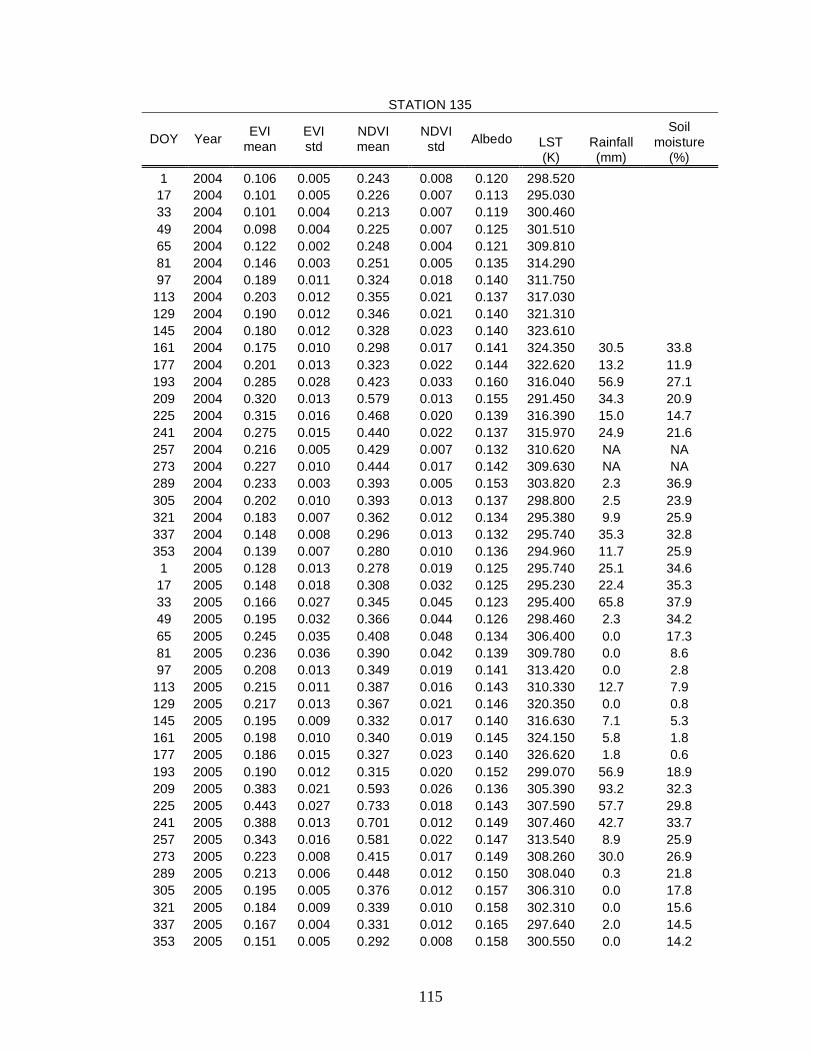
115

STATION 135

DOY Year EVI

mean EVI std

NDVI mean

NDVI std

Albedo LST (K)

Rainfall (mm)

Soil moisture

(%)

1 2004 0.106 0.005 0.243 0.008 0.120 298.520

17 2004 0.101 0.005 0.226 0.007 0.113 295.030

33 2004 0.101 0.004 0.213 0.007 0.119 300.460

49 2004 0.098 0.004 0.225 0.007 0.125 301.510

65 2004 0.122 0.002 0.248 0.004 0.121 309.810

81 2004 0.146 0.003 0.251 0.005 0.135 314.290

97 2004 0.189 0.011 0.324 0.018 0.140 311.750

113 2004 0.203 0.012 0.355 0.021 0.137 317.030

129 2004 0.190 0.012 0.346 0.021 0.140 321.310

145 2004 0.180 0.012 0.328 0.023 0.140 323.610

161 2004 0.175 0.010 0.298 0.017 0.141 324.350 30.5 33.8

177 2004 0.201 0.013 0.323 0.022 0.144 322.620 13.2 11.9

193 2004 0.285 0.028 0.423 0.033 0.160 316.040 56.9 27.1

209 2004 0.320 0.013 0.579 0.013 0.155 291.450 34.3 20.9

225 2004 0.315 0.016 0.468 0.020 0.139 316.390 15.0 14.7

241 2004 0.275 0.015 0.440 0.022 0.137 315.970 24.9 21.6

257 2004 0.216 0.005 0.429 0.007 0.132 310.620 NA NA

273 2004 0.227 0.010 0.444 0.017 0.142 309.630 NA NA

289 2004 0.233 0.003 0.393 0.005 0.153 303.820 2.3 36.9

305 2004 0.202 0.010 0.393 0.013 0.137 298.800 2.5 23.9

321 2004 0.183 0.007 0.362 0.012 0.134 295.380 9.9 25.9

337 2004 0.148 0.008 0.296 0.013 0.132 295.740 35.3 32.8

353 2004 0.139 0.007 0.280 0.010 0.136 294.960 11.7 25.9

1 2005 0.128 0.013 0.278 0.019 0.125 295.740 25.1 34.6

17 2005 0.148 0.018 0.308 0.032 0.125 295.230 22.4 35.3

33 2005 0.166 0.027 0.345 0.045 0.123 295.400 65.8 37.9

49 2005 0.195 0.032 0.366 0.044 0.126 298.460 2.3 34.2

65 2005 0.245 0.035 0.408 0.048 0.134 306.400 0.0 17.3

81 2005 0.236 0.036 0.390 0.042 0.139 309.780 0.0 8.6

97 2005 0.208 0.013 0.349 0.019 0.141 313.420 0.0 2.8

113 2005 0.215 0.011 0.387 0.016 0.143 310.330 12.7 7.9

129 2005 0.217 0.013 0.367 0.021 0.146 320.350 0.0 0.8

145 2005 0.195 0.009 0.332 0.017 0.140 316.630 7.1 5.3

161 2005 0.198 0.010 0.340 0.019 0.145 324.150 5.8 1.8

177 2005 0.186 0.015 0.327 0.023 0.140 326.620 1.8 0.6

193 2005 0.190 0.012 0.315 0.020 0.152 299.070 56.9 18.9

209 2005 0.383 0.021 0.593 0.026 0.136 305.390 93.2 32.3

225 2005 0.443 0.027 0.733 0.018 0.143 307.590 57.7 29.8

241 2005 0.388 0.013 0.701 0.012 0.149 307.460 42.7 33.7

257 2005 0.343 0.016 0.581 0.022 0.147 313.540 8.9 25.9

273 2005 0.223 0.008 0.415 0.017 0.149 308.260 30.0 26.9

289 2005 0.213 0.006 0.448 0.012 0.150 308.040 0.3 21.8

305 2005 0.195 0.005 0.376 0.012 0.157 306.310 0.0 17.8

321 2005 0.184 0.009 0.339 0.010 0.158 302.310 0.0 15.6

337 2005 0.167 0.004 0.331 0.012 0.165 297.640 2.0 14.5

353 2005 0.151 0.005 0.292 0.008 0.158 300.550 0.0 14.2

116

1 2006 0.140 0.005 0.275 0.007 0.163 302.410 0.0 13.6

17 2006 0.139 0.005 0.263 0.009 0.169 301.540 0.0 12.5

33 2006 0.130 0.005 0.255 0.009 0.166 306.260 1.8 12.6

49 2006 0.135 0.004 0.227 0.004 0.165 306.590 2.3 12.7

65 2006 0.134 0.005 0.238 0.007 0.168 307.370 12.2 13.7

81 2006 0.129 0.003 0.237 0.006 0.170 310.560 0.0 19.8

97 2006 0.154 0.011 0.235 0.014 0.174 318.550 0.0 16.0

113 2006 0.165 0.021 0.252 0.027 0.174 319.080 0.0 11.4

129 2006 0.160 0.016 0.263 0.021 0.172 322.530 0.0 9.2

145 2006 0.162 0.015 0.265 0.024 0.170 322.410 3.6 7.9

161 2006 0.175 0.016 0.246 0.016 0.164 326.240 13.7 7.7

177 2006 0.324 0.037 0.454 0.042 0.144 313.450 95.5 33.1

193 2006 0.326 0.026 0.551 0.065 0.142 316.690 32.5 25.6

209 2006 0.489 0.033 0.705 0.025 0.145 289.790 12.4 38.0

225 2006 0.481 0.056 0.685 0.038 0.147 307.180 47.5 36.1

241 2006 0.278 0.036 0.601 0.052 0.146 303.960 52.1 32.6

257 2006 0.357 0.011 0.570 0.008 0.142 308.980 0.0 28.1

273 2006 0.247 0.005 0.499 0.005 0.142 310.260

289 2006 0.175 0.004 0.372 0.007 0.136 305.230

305 2006 0.153 0.004 0.349 0.009 0.134 305.520

321 2006 0.155 0.002 0.345 0.007 0.139 300.900

337 2006 0.141 0.005 0.312 0.012 0.144 298.980

353 2006 0.137 0.004 0.272 0.007 0.142 295.070

9 2007 0.127 0.004 0.234 0.008 0.142 297.64

25 2007 0.107 0.003 0.216 0.009 0.14 NA

33 2007 0.108 0.003 0.217 0.007 0.141 304.59

49 2007 0.121 0.003 0.209 0.007 0.144 305.24

65 2007 0.117 0.004 0.209 0.007 0.15 314.67

81 2007 0.122 0.005 0.231 0.009 0.139 312.86

97 2007 0.157 0.014 0.272 0.021 0.1435 313.5

113 2007 0.183 0.018 0.299 0.024 0.141 318.01

129 2007 0.172 0.012 0.287 0.020 0.145 323.39

145 2007 0.174 0.014 0.302 0.025 0.149 323.96

161 2007 0.203 0.024 0.356 0.067 0.145 327.18

177 2007 0.483 0.057 0.640 0.046 0.152 330.58

193 2007 0.518 0.040 0.680 0.029 NA 311.38

209 2007 0.467 0.027 0.706 0.021 0.1705 308.65

225 2007 0.354 0.018 0.649 0.016 0.144 NA

117

STATION 136

DOY Year EVI

mean EVI std

NDVI mean

NDVI std

Albedo LST (K)

Rainfall (mm)

Soil moisture

(%)

1 2004 0.127 0.005 0.269 0.020 0.130 296.120

17 2004 0.129 0.007 0.274 0.024 0.121 293.980

33 2004 0.131 0.004 0.279 0.027 0.127 301.080

49 2004 0.129 0.003 0.258 0.015 0.127 300.000

65 2004 0.140 0.005 0.292 0.018 0.127 307.210

81 2004 0.171 0.006 0.294 0.017 0.135 312.170

97 2004 0.177 0.007 0.321 0.019 0.134 309.020

113 2004 0.166 0.012 0.294 0.015 0.136 315.790 0.0 0.0

129 2004 0.142 0.012 0.277 0.020 0.141 319.610 0.0 0.0

145 2004 0.129 0.009 0.249 0.019 0.138 322.280 0.0 0.0

161 2004 0.124 0.009 0.229 0.016 0.141 322.300 5.6 0.8

177 2004 0.131 0.007 0.238 0.010 0.136 322.410 0.5 1.0

193 2004 0.270 0.013 0.424 0.018 0.146 315.340 12.7 6.6

209 2004 0.411 0.019 0.575 0.017 0.147 306.850 8.4 6.3

225 2004 0.375 0.008 0.553 0.014 0.142 314.620 21.3 2.2

241 2004 0.329 0.012 0.598 0.017 0.139 314.460 27.2 2.2

257 2004 0.302 0.019 0.556 0.014 0.136 310.720 NA NA

273 2004 0.312 0.010 0.594 0.016 0.139 308.750 NA NA

289 2004 0.274 0.007 0.461 0.015 0.141 302.220 1.3 3.4

305 2004 0.251 0.009 0.476 0.022 0.133 299.450 5.8 0.6

321 2004 0.219 0.008 0.455 0.025 0.131 294.270 8.9 1.3

337 2004 0.197 0.009 0.396 0.026 0.129 295.330 31.8 2.5

353 2004 0.198 0.010 0.377 0.021 0.130 294.540 14.5 1.0

1 2005 0.186 0.009 0.394 0.025 0.127 297.310 16.5 5.0

17 2005 0.182 0.010 0.372 0.019 0.123 297.250 25.4 3.6

33 2005 0.171 0.007 0.347 0.018 0.121 295.490 39.1 4.4

49 2005 0.188 0.006 0.362 0.012 0.126 297.390 7.1 2.5

65 2005 0.199 0.009 0.364 0.018 0.130 304.880 4.1 0.3

81 2005 0.187 0.009 0.348 0.016 0.132 309.050 0.0 0.0

97 2005 0.171 0.011 0.314 0.021 0.140 312.970 0.5 0.0

113 2005 0.170 0.012 0.311 0.035 0.139 311.750 6.4 0.1

129 2005 0.153 0.011 0.292 0.009 0.141 319.560 0.0 0.0

145 2005 0.202 0.009 0.377 0.016 0.136 317.370 50.8 1.1

161 2005 0.187 0.009 0.352 0.011 0.137 321.230 5.8 0.3

177 2005 0.176 0.006 0.334 0.013 0.138 324.870 0.0 0.0

193 2005 0.237 0.073 0.405 0.117 0.131 317.210 77.5 2.8

209 2005 0.420 0.037 0.623 0.050 0.144 306.610 100.6 1.2

225 2005 0.433 0.012 0.727 0.018 0.138 310.490 29.7 0.0

241 2005 0.283 0.013 0.570 0.026 0.136 306.900 23.1 0.0

257 2005 0.259 0.022 0.480 0.017 0.136 315.110 23.9 0.0

273 2005 0.222 0.013 0.404 0.029 0.138 311.110 15.2 0.0

289 2005 0.189 0.014 0.393 0.036 0.139 308.540 0.3 0.0

305 2005 0.185 0.011 0.354 0.038 0.137 307.640 0.0 0.0

321 2005 0.169 0.012 0.316 0.034 0.141 303.170 0.0 0.0

337 2005 0.160 0.012 0.336 0.030 0.144 299.070 0.8 0.0

353 2005 0.149 0.011 0.294 0.023 0.138 301.290 0.0 0.0

118

1 2006 0.140 0.007 0.291 0.022 0.143 303.410 0.0 0.0

17 2006 0.139 0.007 0.286 0.024 0.145 300.500 0.0 0.0

33 2006 0.128 0.007 0.264 0.016 0.140 306.450 2.3 0.0

49 2006 0.136 0.006 0.234 0.014 0.143 306.130 0.0 0.0

65 2006 0.126 0.009 0.249 0.016 0.148 305.760 5.6 0.0

81 2006 0.120 0.006 0.238 0.012 0.147 311.080 0.0 0.0

97 2006 0.131 0.004 0.209 0.010 0.149 317.420 0.0 0.0

113 2006 0.124 0.012 0.218 0.008 0.154 317.750 0.0 0.0

129 2006 0.117 0.006 0.213 0.009 0.151 323.530 0.0 0.0

145 2006 0.132 0.008 0.213 0.007 0.152 323.560 3.6 0.0

161 2006 0.125 0.012 0.213 0.006 0.150 324.990 10.2 0.0

177 2006 0.230 0.012 0.368 0.022 0.128 314.160 100.6 2.4

193 2006 0.249 0.017 0.431 0.014 0.142 318.400 31.2 6.8

209 2006 0.481 0.015 0.711 0.016 0.152 286.450 33.0 10.9

225 2006 0.387 0.015 0.628 0.028 0.148 306.960 20.8 7.8

241 2006 0.367 0.048 0.453 0.054 0.133 303.720 112.0 9.2

257 2006 0.405 0.006 0.632 0.018 0.136 307.030 0.0 6.0

273 2006 0.295 0.010 0.562 0.019 0.146 309.550

289 2006 0.227 0.005 0.461 0.025 0.135 303.550

305 2006 0.215 0.007 0.452 0.025 0.134 304.870

321 2006 0.192 0.005 0.399 0.016 0.137 300.740

337 2006 0.174 0.009 0.351 0.018 0.143 298.400

353 2006 0.158 0.007 0.318 0.019 0.138 294.820

9 2007 0.143 0.005 0.284 0.016 0.1355 296.81

25 2007 0.130 0.004 0.275 0.022 0.1385 NA

33 2007 0.132 0.002 0.271 0.017 0.1325 301.34

49 2007 0.126 0.006 0.243 0.016 0.1355 302.3

65 2007 0.120 0.006 0.257 0.021 0.1395 312.98

81 2007 0.133 0.005 0.278 0.014 0.136 309.34

97 2007 0.138 0.008 0.256 0.019 0.14 310.68

113 2007 0.128 0.005 0.258 0.020 0.1415 315.53

129 2007 0.123 0.003 0.233 0.015 0.1415 320.99

145 2007 0.118 0.006 0.238 0.016 0.1425 322.06

161 2007 0.221 0.006 0.450 0.014 0.1385 324.45

177 2007 0.436 0.039 0.633 0.055 0.1405 328.81

193 2007 0.510 0.016 0.771 0.011 0.15 311.18

209 2007 0.358 0.011 0.616 0.017 0.143 306.71

225 2007 0.306 0.018 0.594 0.016 0.132 NA

119

STATION 137

DOY Year EVI

mean EVI std

NDVI mean

NDVI std

Albedo LST (K)

Rainfall (mm)

Soil moisture

(%)

1 2004 0.144 0.008 0.255 0.007 0.152 300.580

17 2004 0.134 0.003 0.233 0.004 0.134 297.280

33 2004 0.130 0.006 0.224 0.003 0.143 302.520

49 2004 0.130 0.003 0.209 0.002 0.146 301.170

65 2004 0.125 0.004 0.212 0.003 0.144 311.170

81 2004 0.133 0.004 0.207 0.003 0.149 318.300

97 2004 0.139 0.009 0.214 0.005 0.148 316.280

113 2004 0.129 0.007 0.207 0.006 0.154 321.150

129 2004 0.126 0.006 0.208 0.004 0.157 323.650

145 2004 0.119 0.003 0.200 0.003 0.158 326.150

161 2004 0.118 0.005 0.194 0.003 0.157 326.270

177 2004 0.133 0.004 0.202 0.006 0.161 328.320 3.3 3.4

193 2004 0.203 0.014 0.279 0.020 0.178 316.030 97.3 7.1

209 2004 0.353 0.043 0.517 0.036 0.160 312.940 37.1 3.4

225 2004 0.283 0.027 0.408 0.030 0.156 317.170 28.4 7.5

241 2004 0.273 0.012 0.414 0.023 0.158 316.120 43.4 9.5

257 2004 0.229 0.009 0.362 0.012 0.157 312.860 NA NA

273 2004 0.192 0.006 0.323 0.008 0.158 314.780 NA NA

289 2004 0.166 0.003 0.291 0.003 0.163 307.400 52.6 9.4

305 2004 0.176 0.006 0.292 0.009 0.146 300.710 20.8 6.0

321 2004 0.184 0.007 0.329 0.010 0.139 295.860 7.9 15.0

337 2004 0.189 0.007 0.321 0.010 0.140 296.650 24.9 19.0

353 2004 0.185 0.006 0.307 0.005 0.150 284.500 21.8 12.6

1 2005 0.185 0.017 0.330 0.019 0.140 297.150 28.4 24.1

17 2005 0.204 0.028 0.350 0.042 0.143 298.130 21.8 22.3

33 2005 0.205 0.030 0.355 0.040 0.141 296.510 70.1 25.4

49 2005 0.219 0.030 0.337 0.038 0.151 297.410 4.3 20.4

65 2005 0.215 0.026 0.350 0.030 0.153 307.860 0.3 2.7

81 2005 0.205 0.014 0.322 0.018 0.152 310.920 0.0 0.0

97 2005 0.192 0.007 0.293 0.013 0.158 315.430 0.0 0.0

113 2005 0.170 0.006 0.286 0.006 0.152 314.850 7.4 1.6

129 2005 0.164 0.007 0.269 0.007 0.163 323.990 NA NA

145 2005 0.170 0.011 0.260 0.003 0.158 322.370 NA NA

161 2005 0.157 0.006 0.232 0.006 0.159 325.240 NA NA

177 2005 0.156 0.005 0.230 0.004 0.158 329.360 NA NA

193 2005 0.145 0.002 0.218 0.004 0.190 322.560 NA NA

209 2005 0.315 0.016 0.512 0.040 0.166 310.550 NA NA

225 2005 0.361 0.023 0.564 0.017 0.153 312.700 NA NA

241 2005 0.311 0.020 0.423 0.021 0.143 314.460 NA NA

257 2005 0.233 0.007 0.400 0.008 0.153 318.280 NA NA

273 2005 0.226 0.004 0.320 0.003 0.158 315.830 NA NA

289 2005 0.175 0.006 0.299 0.004 0.166 311.990 NA NA

305 2005 0.178 0.007 0.278 0.007 0.166 309.410 NA NA

321 2005 0.173 0.006 0.268 0.006 0.168 305.850 0.0 0.0

337 2005 0.161 0.006 0.270 0.006 0.167 300.920 1.5 0.0

353 2005 0.159 0.006 0.253 0.005 0.166 302.950 0.0 0.0

120

1 2006 0.144 0.005 0.244 0.003 0.168 305.160 0.0 0.0

17 2006 0.150 0.006 0.240 0.004 0.168 302.890 0.0 0.0

33 2006 0.136 0.004 0.225 0.004 0.166 309.200 0.0 0.0

49 2006 0.140 0.004 0.207 0.003 0.166 307.940 2.5 0.0

65 2006 0.146 0.003 0.211 0.001 0.169 308.610 5.1 0.0

81 2006 0.127 0.004 0.203 0.003 0.170 315.250 0.0 0.0

97 2006 0.134 0.005 0.189 0.002 0.174 319.790 0.0 0.0

113 2006 0.132 0.003 0.187 0.002 0.176 319.540 0.0 0.0

129 2006 0.123 0.003 0.190 0.004 0.177 326.100 0.0 0.0

145 2006 0.126 0.006 0.184 0.002 0.185 325.610 3.6 0.0

161 2006 0.125 0.002 0.189 0.003 0.174 328.660 8.9 0.0

177 2006 0.235 0.031 0.303 0.029 0.160 316.890 108.5 13.8

193 2006 0.364 0.029 0.520 0.020 0.167 316.280 NA NA

209 2006 0.443 0.016 0.634 0.011 0.155 290.200 NA NA

225 2006 0.429 0.025 0.599 0.018 0.162 307.640 44.7 22.9

241 2006 0.407 0.018 0.618 0.022 0.151 306.870 82.0 29.0

257 2006 0.410 0.010 0.580 0.007 0.151 310.050 0.0 21.2

273 2006 0.253 0.014 0.435 0.030 0.152 310.570

289 2006 0.211 0.009 0.374 0.009 0.145 305.320

305 2006 0.203 0.009 0.370 0.009 0.144 305.850

321 2006 0.198 0.008 0.363 0.007 0.147 301.740

337 2006 0.171 0.007 0.322 0.007 0.151 299.110

353 2006 0.173 0.006 0.296 0.007 0.146 295.540

9 2007 0.158 0.009 0.270 0.010 0.147 298.060

25 2007 0.128 0.007 0.240 0.009 0.138 NA

33 2007 0.137 0.006 0.237 0.006 0.142 303.780

49 2007 0.137 0.004 0.225 0.004 0.148 305.560

65 2007 0.125 0.003 0.229 0.003 0.148 314.950

81 2007 0.145 0.007 0.242 0.006 0.146 313.240

97 2007 0.148 0.009 0.230 0.007 0.153 314.660

113 2007 0.150 0.008 0.230 0.004 0.152 318.930

129 2007 0.139 0.006 0.217 0.005 0.155 323.890

145 2007 0.158 0.006 0.261 0.009 0.159 324.760

161 2007 0.179 0.002 0.237 0.002 0.159 326.210

177 2007 0.321 0.019 0.471 0.022 0.163 329.790

193 2007 0.338 0.012 0.540 0.013

NA 320.290

209 2007 0.340 0.020 0.520 0.022 0.156 310.390

225 2007 0.284 0.011 0.474 0.018 0.159 NA

121

STATION 138

DOY Year EVI

mean EVI std

NDVI mean

NDVI std

Albedo LST (K)

Rainfall (mm)

Soil moisture

(%)

1 2004 0.149 0.009 0.284 0.019 0.143 299.020

17 2004 0.136 0.010 0.254 0.018 0.137 295.440

33 2004 0.135 0.009 0.247 0.012 0.142 301.880

49 2004 0.112 0.004 0.227 0.009 0.153 299.410

65 2004 0.123 0.005 0.230 0.010 0.143 312.510

81 2004 0.131 0.006 0.216 0.013 0.146 314.350

97 2004 0.159 0.013 0.259 0.019 0.149 313.180

113 2004 0.158 0.015 0.253 0.021 0.154 321.320

129 2004 0.145 0.013 0.243 0.017 0.159 323.810

145 2004 0.146 0.013 0.209 0.019 0.161 326.490

161 2004 0.137 0.013 0.218 0.017 0.162 326.970 25.1 21.1

177 2004 0.149 0.009 0.234 0.008 0.161 327.230 7.1 13.4

193 2004 0.184 0.010 0.276 0.014 0.183 324.050 69.6 19.0

209 2004 0.259 0.018 0.417 0.031 0.173 295.400 3.8 14.8

225 2004 0.213 0.013 0.300 0.019 0.157 319.370 7.9 8.8

241 2004 0.217 0.024 0.319 0.024 0.155 319.090 42.7 13.9

257 2004 0.214 0.010 0.362 0.021 0.152 316.080 NA NA

273 2004 0.196 0.015 0.334 0.019 0.154 314.890 NA NA

289 2004 0.181 0.010 0.314 0.015 0.148 306.800 48.0 8.8

305 2004 0.193 0.013 0.320 0.022 0.141 301.690 18.0 16.6

321 2004 0.189 0.012 0.327 0.024 0.136 296.100 6.4 20.0

337 2004 0.163 0.009 0.301 0.015 0.137 297.680 26.4 20.9

353 2004 0.156 0.009 0.285 0.011 0.144 296.330 20.3 17.5

1 2005 0.160 0.014 0.304 0.005 0.134 298.250 24.9 22.4

17 2005 0.167 0.010 0.310 0.021 0.135 297.880 17.0 21.6

33 2005 0.170 0.015 0.327 0.022 0.135 297.450 68.3 24.1

49 2005 0.201 0.017 0.333 0.025 0.148 302.260 0.8 19.3

65 2005 0.209 0.019 0.335 0.023 0.147 308.860 1.0 11.6

81 2005 0.202 0.014 0.326 0.018 0.155 310.600 0.0 8.3

97 2005 0.187 0.013 0.295 0.018 0.156 316.000 0.0 7.0

113 2005 0.181 0.013 0.293 0.012 0.157 314.030 8.1 10.6

129 2005 0.167 0.011 0.275 0.013 0.163 322.110 1.3 6.8

145 2005 0.157 0.013 0.260 0.016 0.160 324.750 0.0 6.5

161 2005 0.152 0.011 0.243 0.016 0.164 326.550 1.5 6.5

177 2005 0.159 0.009 0.250 0.017 0.161 330.300 0.5 7.4

193 2005 0.146 0.013 0.221 0.014 0.185 300.490 43.4 10.7

209 2005 0.215 0.009 0.408 0.018 0.154 292.580 82.0 22.9

225 2005 0.368 0.029 0.579 0.028 0.149 313.330 61.7 17.2

241 2005 0.316 0.029 0.555 0.042 0.155 312.270 46.5 17.7

257 2005 0.271 0.020 0.456 0.020 0.157 317.450 3.3 10.3

273 2005 0.217 0.012 0.325 0.016 0.160 314.540 1.3 7.6

289 2005 0.192 0.012 0.333 0.012 0.164 311.260 0.0 6.9

305 2005 0.182 0.017 0.301 0.019 0.163 309.950 NA NA

321 2005 0.183 0.008 0.295 0.014 0.163 305.330 0.0 5.0

122

337 2005 0.172 0.013 0.293 0.012 0.162 300.920 1.0 4.7

353 2005 0.153 0.007 0.260 0.010 0.161 302.680 0.0 4.8

1 2006 0.145 0.008 0.255 0.007 0.164 304.230 0.0 4.6

17 2006 0.142 0.006 0.240 0.007 0.160 302.980 0.0 4.2

33 2006 0.131 0.008 0.228 0.011 0.167 308.900 0.0 4.6

49 2006 0.131 0.006 0.207 0.011 0.166 310.390 3.0 5.4

65 2006 0.127 0.008 0.212 0.012 0.166 310.800 3.0 4.9

81 2006 0.122 0.006 0.209 0.009 0.172 315.520 0.0 5.3

97 2006 0.135 0.009 0.206 0.010 0.179 321.430 0.0 5.0

113 2006 0.131 0.008 0.199 0.011 0.181 321.130 0.0 4.8

129 2006 0.122 0.007 0.195 0.007 0.178 327.780 0.0 5.0

145 2006 0.132 0.010 0.193 0.013 0.177 327.270 3.6 5.2

161 2006 0.123 0.011 0.191 0.015 0.177 330.980 6.4 5.7

177 2006 0.274 0.040 0.355 0.042 0.156 318.750 100.8 19.4

193 2006 0.357 0.088 0.520 0.096 0.156 316.120 78.5 16.9

209 2006 0.463 0.044 0.666 0.047 0.155 305.340 86.6 20.6

225 2006 0.490 0.048 0.652 0.050 0.159 309.430 30.2 17.2

241 2006 0.426 0.050 0.634 0.059 0.155 307.350 108.5 20.9

257 2006 0.392 0.033 0.577 0.039 0.155 309.840 1.8 15.4

273 2006 0.309 0.024 0.526 0.036 0.152 311.100 5.3 11.4

289 2006 0.234 0.015 0.434 0.030 0.138 306.210

305 2006 0.212 0.011 0.401 0.029 0.142 304.980

321 2006 0.205 0.012 0.390 0.024 0.142 301.540

337 2006 0.174 0.006 0.343 0.014 0.144 298.460

353 2006 0.159 0.005 0.298 0.010 0.144 294.960

9 2007 0.137 0.003 0.243 0.006 0.157 296.380

25 2007 0.104 0.005 0.212 0.008 0.148 NA

33 2007 0.115 0.009 0.215 0.008 0.146 303.170

49 2007 0.115 0.005 0.203 0.006 0.150 304.170

65 2007 0.131 0.007 0.253 0.013 0.156 314.100

81 2007 0.159 0.015 0.280 0.013 0.154 310.970

97 2007 0.165 0.021 0.270 0.028 0.158 313.370

113 2007 0.166 0.019 0.267 0.026 0.160 318.000

129 2007 0.168 0.014 0.249 0.020 0.160 322.670

145 2007 0.163 0.015 0.255 0.015 0.167 324.480

161 2007 0.168 0.015 0.227 0.016 0.162 327.950

177 2007 0.304 0.023 0.468 0.028 0.165 329.970

193 2007 0.409 0.030 0.603 0.031 NA NA

209 2007 0.392 0.037 0.602 0.038 0.156 312.680

225 2007 0.349 0.027 0.560 0.020 0.151 NA

123

STATION 139

DOY Year EVI

mean EVI std

NDVI mean

NDVI std

Albedo LST (K)

Rainfall (mm)

Soil moisture

(%)

1 2004 0.119 0.008 0.229 0.016 0.142 298.060

17 2004 0.112 0.015 0.205 0.021 0.136 296.490

33 2004 0.112 0.013 0.199 0.018 0.139 300.500

49 2004 0.111 0.012 0.199 0.016 0.135 298.080

65 2004 0.113 0.008 0.200 0.013 0.136 308.450

81 2004 0.120 0.007 0.191 0.011 0.142 317.630

97 2004 0.149 0.007 0.222 0.014 0.144 314.390

113 2004 0.143 0.006 0.236 0.011 0.148 320.020

129 2004 0.139 0.010 0.223 0.010 0.154 321.320

145 2004 0.129 0.009 0.183 0.009 0.151 326.160

161 2004 0.117 0.003 0.169 0.007 0.153 325.580 17.5 15.2

177 2004 0.136 0.008 0.185 0.011 0.141 326.780 8.6 8.2

193 2004 0.166 0.019 0.239 0.028 0.178 318.890 132.8 12.2

209 2004 0.255 0.027 0.390 0.037 0.162 312.230 40.4 10.1

225 2004 0.264 0.037 0.394 0.053 0.155 311.680 24.4 9.1

241 2004 0.250 0.028 0.392 0.039 0.153 317.190 37.1 9.5

257 2004 0.237 0.026 0.372 0.038 0.144 313.870 NA NA

273 2004 0.199 0.012 0.341 0.024 0.155 313.250 NA NA

289 2004 0.174 0.007 0.299 0.012 0.143 305.600 15.7 16.4

305 2004 0.159 0.011 0.275 0.018 0.136 301.710 12.4 7.4

321 2004 0.168 0.014 0.286 0.020 0.133 295.830 2.5 7.9

337 2004 0.145 0.019 0.258 0.032 0.132 296.240 28.2 11.1

353 2004 0.145 0.019 0.250 0.032 0.130 297.030 16.8 6.5

1 2005 0.132 0.028 0.246 0.030 0.130 295.730 37.8 14.5

17 2005 0.151 0.024 0.272 0.035 0.130 297.190 13.0 11.8

33 2005 0.153 0.028 0.299 0.038 0.129 296.980 71.9 15.3

49 2005 0.195 0.028 0.329 0.040 0.142 299.230 1.5 9.5

65 2005 0.221 0.026 0.351 0.032 0.141 306.540 0.3 5.3

81 2005 0.213 0.015 0.341 0.019 0.143 310.310 0.0 3.8

97 2005 0.190 0.006 0.292 0.013 0.148 315.660 0.0 3.1

113 2005 0.168 0.014 0.278 0.028 0.145 314.090 4.1 4.0

129 2005 0.160 0.009 0.264 0.011 0.152 323.420 0.0 2.9

145 2005 0.152 0.011 0.260 0.021 0.149 322.160 2.3 3.2

161 2005 0.153 0.012 0.255 0.021 0.151 326.220 1.8 3.0

177 2005 0.151 0.005 0.229 0.010 0.147 326.500 3.6 3.2

193 2005 0.135 0.004 0.213 0.006 0.174 310.810 64.3 7.8

209 2005 0.230 0.031 0.394 0.050 0.162 273.000 54.4 8.7

225 2005 0.232 0.021 0.368 0.026 0.141 314.830 29.0 6.6

241 2005 0.254 0.019 0.452 0.032 0.144 313.360 42.4 6.7

257 2005 0.215 0.015 0.359 0.014 0.148 317.960 3.6 3.5

273 2005 0.187 0.014 0.278 0.017 0.147 314.070 4.6 2.6

289 2005 0.161 0.012 0.289 0.015 0.147 310.850 0.0 4.3

305 2005 0.171 0.009 0.272 0.015 0.150 309.810 NA NA

321 2005 0.168 0.012 0.266 0.017 0.152 304.830 0.0 1.1

337 2005 0.145 0.014 0.266 0.014 0.162 300.510 1.0 0.9

353 2005 0.135 0.007 0.234 0.014 0.151 303.740 0.0 0.9

124

1 2006 0.130 0.009 0.229 0.012 0.153 304.010 0.0 0.8

17 2006 0.129 0.006 0.232 0.012 0.155 302.720 0.0 0.7

33 2006 0.119 0.006 0.210 0.010 0.150 308.370 0.0 0.9

49 2006 0.084 0.018 0.185 0.010 0.159 308.610 1.3 1.2

65 2006 0.115 0.008 0.200 0.012 0.157 308.060 6.1 1.4

81 2006 0.113 0.008 0.198 0.010 0.161 313.570 0.0 2.6

97 2006 0.133 0.015 0.211 0.014 0.165 320.130 0.0 1.4

113 2006 0.121 0.009 0.207 0.017 0.167 320.980 0.0 1.2

129 2006 0.118 0.008 0.194 0.010 0.167 326.390 0.0 1.5

145 2006 0.116 0.011 0.187 0.015 0.166 326.630 1.3 1.6

161 2006 0.121 0.011 0.194 0.013 0.164 329.430 10.2 2.7

177 2006 0.178 0.020 0.258 0.027 0.160 316.750 125.2 14.1

193 2006 0.253 0.041 0.383 0.049 0.151 315.750 61.7 11.0

209 2006 0.489 0.053 0.654 0.041 0.155 307.700 50.8 18.1

225 2006 0.463 0.054 0.631 0.050 0.151 305.790 69.6 13.1

241 2006 0.419 0.045 0.614 0.046 0.148 305.480 100.6 14.1

257 2006 0.428 0.024 0.594 0.029 0.147 307.810 0.3 5.1

273 2006 0.303 0.014 0.511 0.020 0.147 309.330 0.5 3.4

289 2006 0.221 0.009 0.420 0.021 0.133 302.930

305 2006 0.201 0.016 0.393 0.029 0.130 303.620

321 2006 0.197 0.006 0.385 0.014 0.133 300.150

337 2006 0.158 0.011 0.332 0.018 0.137 298.380

353 2006 0.161 0.009 0.296 0.012 0.135 295.290

9 2007 0.139 0.008 0.244 0.014 0.141 297.020

25 2007 0.111 0.008 0.226 0.013 0.134 NA

33 2007 0.114 0.008 0.220 0.011 0.134 302.890

49 2007 0.117 0.006 0.210 0.012 0.139 304.990

65 2007 0.149 0.003 0.249 0.008 0.140 314.610

81 2007 0.155 0.012 0.285 0.007 0.139 310.970

97 2007 0.159 0.008 0.271 0.013 0.144 312.150

113 2007 0.162 0.009 0.268 0.016 0.150 318.110

129 2007 0.157 0.011 0.257 0.016 0.152 322.440

145 2007 0.156 0.011 0.255 0.021 0.151 324.500

161 2007 0.149 0.005 0.273 0.010 0.151 327.770

177 2007 0.229 0.027 0.364 0.032 0.156 331.530

193 2007 0.385 0.026 0.533 0.031 NA NA

209 2007 0.430 0.038 0.640 0.035 0.158 309.170

225 2007 0.390 0.025 0.620 0.021 0.151 NA

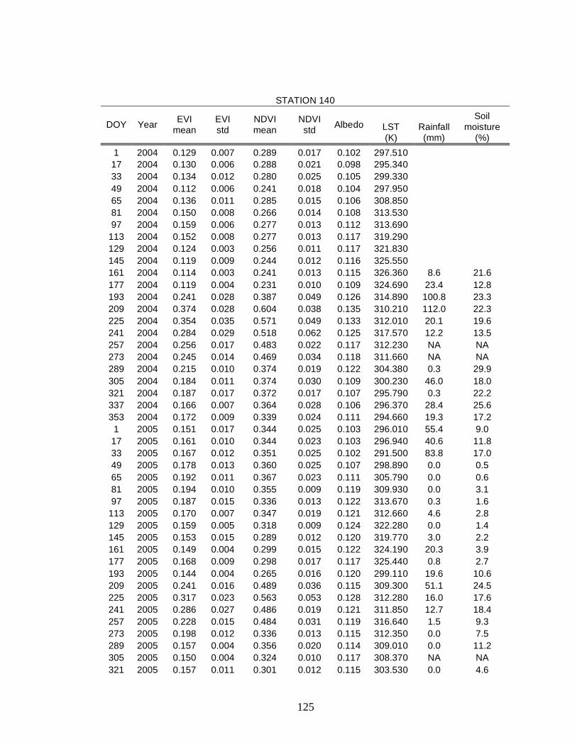
125

STATION 140

DOY Year EVI

mean EVI std

NDVI mean

NDVI std

Albedo LST (K)

Rainfall (mm)

Soil moisture

(%)

1 2004 0.129 0.007 0.289 0.017 0.102 297.510

17 2004 0.130 0.006 0.288 0.021 0.098 295.340

33 2004 0.134 0.012 0.280 0.025 0.105 299.330

49 2004 0.112 0.006 0.241 0.018 0.104 297.950

65 2004 0.136 0.011 0.285 0.015 0.106 308.850

81 2004 0.150 0.008 0.266 0.014 0.108 313.530

97 2004 0.159 0.006 0.277 0.013 0.112 313.690

113 2004 0.152 0.008 0.277 0.013 0.117 319.290

129 2004 0.124 0.003 0.256 0.011 0.117 321.830

145 2004 0.119 0.009 0.244 0.012 0.116 325.550

161 2004 0.114 0.003 0.241 0.013 0.115 326.360 8.6 21.6

177 2004 0.119 0.004 0.231 0.010 0.109 324.690 23.4 12.8

193 2004 0.241 0.028 0.387 0.049 0.126 314.890 100.8 23.3

209 2004 0.374 0.028 0.604 0.038 0.135 310.210 112.0 22.3

225 2004 0.354 0.035 0.571 0.049 0.133 312.010 20.1 19.6

241 2004 0.284 0.029 0.518 0.062 0.125 317.570 12.2 13.5

257 2004 0.256 0.017 0.483 0.022 0.117 312.230 NA NA

273 2004 0.245 0.014 0.469 0.034 0.118 311.660 NA NA

289 2004 0.215 0.010 0.374 0.019 0.122 304.380 0.3 29.9

305 2004 0.184 0.011 0.374 0.030 0.109 300.230 46.0 18.0

321 2004 0.187 0.017 0.372 0.017 0.107 295.790 0.3 22.2

337 2004 0.166 0.007 0.364 0.028 0.106 296.370 28.4 25.6

353 2004 0.172 0.009 0.339 0.024 0.111 294.660 19.3 17.2

1 2005 0.151 0.017 0.344 0.025 0.103 296.010 55.4 9.0

17 2005 0.161 0.010 0.344 0.023 0.103 296.940 40.6 11.8

33 2005 0.167 0.012 0.351 0.025 0.102 291.500 83.8 17.0

49 2005 0.178 0.013 0.360 0.025 0.107 298.890 0.0 0.5

65 2005 0.192 0.011 0.367 0.023 0.111 305.790 0.0 0.6

81 2005 0.194 0.010 0.355 0.009 0.119 309.930 0.0 3.1

97 2005 0.187 0.015 0.336 0.013 0.122 313.670 0.3 1.6

113 2005 0.170 0.007 0.347 0.019 0.121 312.660 4.6 2.8

129 2005 0.159 0.005 0.318 0.009 0.124 322.280 0.0 1.4

145 2005 0.153 0.015 0.289 0.012 0.120 319.770 3.0 2.2

161 2005 0.149 0.004 0.299 0.015 0.122 324.190 20.3 3.9

177 2005 0.168 0.009 0.298 0.017 0.117 325.440 0.8 2.7

193 2005 0.144 0.004 0.265 0.016 0.120 299.110 19.6 10.6

209 2005 0.241 0.016 0.489 0.036 0.115 309.300 51.1 24.5

225 2005 0.317 0.023 0.563 0.053 0.128 312.280 16.0 17.6

241 2005 0.286 0.027 0.486 0.019 0.121 311.850 12.7 18.4

257 2005 0.228 0.015 0.484 0.031 0.119 316.640 1.5 9.3

273 2005 0.198 0.012 0.336 0.013 0.115 312.350 0.0 7.5

289 2005 0.157 0.004 0.356 0.020 0.114 309.010 0.0 11.2

305 2005 0.150 0.004 0.324 0.010 0.117 308.370 NA NA

321 2005 0.157 0.011 0.301 0.012 0.115 303.530 0.0 4.6

126

337 2005 0.137 0.003 0.304 0.014 0.115 299.730 0.0 4.4

353 2005 0.137 0.009 0.279 0.014 0.113 302.060 0.0 4.5

1 2006 0.127 0.005 0.275 0.013 0.115 302.660 0.0 4.1

17 2006 0.127 0.007 0.261 0.019 0.114 301.850 0.0 3.9

33 2006 0.119 0.004 0.264 0.015 0.114 307.300 0.0 4.0

49 2006 0.123 0.006 0.225 0.012 0.115 307.970 0.0 4.2

65 2006 0.112 0.005 0.238 0.011 0.118 306.890 0.0 4.2

81 2006 0.110 0.004 0.228 0.013 0.123 313.510 0.0 4.7

97 2006 0.123 0.003 0.209 0.010 0.121 319.010 0.0 4.0

113 2006 0.123 0.006 0.211 0.011 0.123 319.730 0.0 3.7

129 2006 0.114 0.007 0.209 0.013 0.121 326.980 0.0 3.6

145 2006 0.119 0.007 0.216 0.012 0.119 325.900 0.0 3.6

161 2006 0.110 0.004 0.214 0.010 0.121 326.460 0.0 8.8

177 2006 0.267 0.029 0.410 0.046 0.122 312.290 24.9 24.0

193 2006 0.334 0.033 0.615 0.054 0.127 313.380 0.5 26.9

209 2006 0.477 0.062 0.688 0.063 0.140 306.550 NA NA

225 2006 0.420 0.064 0.649 0.076 0.143 305.970 2.5 32.8

241 2006 0.408 0.077 0.643 0.089 0.137 305.800 98.0 33.2

257 2006 0.333 0.057 0.547 0.080 0.129 310.510 26.9 16.6

273 2006 0.245 0.019 0.476 0.033 0.119 310.120 0.0 13.3

289 2006 0.183 0.018 0.381 0.037 0.115 305.230

305 2006 0.177 0.013 0.367 0.024 0.116 304.960

321 2006 0.167 0.013 0.356 0.027 0.117 301.160

337 2006 0.158 0.013 0.342 0.028 0.121 298.100

353 2006 0.161 0.010 0.317 0.029 0.113 293.810

9 2007 0.144 0.010 0.286 0.021 0.120 297.130

25 2007 0.125 0.009 0.274 0.022 0.114 NA

33 2007 0.132 0.010 0.280 0.024 0.115 302.080

49 2007 0.123 0.009 0.255 0.023 0.117 304.180

65 2007 0.114 0.003 0.278 0.015 0.119 313.240

81 2007 0.126 0.005 0.272 0.018 0.117 311.820

97 2007 0.132 0.005 0.260 0.017 0.122 312.520

113 2007 0.129 0.004 0.252 0.015 0.123 318.260

129 2007 0.136 0.008 0.243 0.014 0.123 322.310

145 2007 0.118 0.005 0.238 0.009 0.120 324.290

161 2007 0.162 0.005 0.360 0.019 0.122 325.800

177 2007 0.325 0.020 0.539 0.030 0.111 330.000

193 2007 0.409 0.025 0.601 0.025 0.134 315.920

209 2007 0.394 0.043 0.626 0.040 0.137 307.570

225 2007 0.370 0.040 0.637 0.046 0.138 NA

127

STATION 143

DOY Year EVI

mean EVI std

NDVI mean

NDVI std

Albedo LST (K)

Rainfall (mm)

Soil moisture

(%)

1 2004 0.103 0.003 0.227 0.005 0.136 297.900

17 2004 0.096 0.005 0.208 0.008 0.121 295.990

33 2004 0.102 0.004 0.201 0.005 0.132 301.250

49 2004 0.108 0.004 0.215 0.007 0.135 301.720

65 2004 0.159 0.013 0.294 0.018 0.133 307.650

81 2004 0.165 0.010 0.272 0.013 0.143 315.680

97 2004 0.208 0.011 0.332 0.019 0.142 311.840

113 2004 0.215 0.011 0.347 0.018 0.147 318.240

129 2004 0.198 0.009 0.339 0.012 0.152 321.910

145 2004 0.179 0.008 0.309 0.009 0.148 324.810

161 2004 0.184 0.010 0.291 0.013 0.152 324.700 15.7 6.3

177 2004 0.180 0.011 0.283 0.013 0.150 324.720 2.8 7.9

193 2004 0.246 0.017 0.349 0.019 0.161 317.330 87.1 18.6

209 2004 0.363 0.020 0.579 0.028 0.167 311.600 20.6 12.0

225 2004 0.311 0.022 0.459 0.023 0.153 316.730 17.8 13.6

241 2004 0.265 0.030 0.405 0.033 0.142 317.570 25.9 11.1

257 2004 0.237 0.022 0.396 0.021 0.142 312.850 NA 0.0

273 2004 0.247 0.011 0.418 0.022 0.144 311.750 0.0 0.0

289 2004 0.235 0.013 0.372 0.014 0.127 302.350 1.3 1.5

305 2004 0.182 0.004 0.349 0.008 0.138 299.480 5.8 2.0

321 2004 0.165 0.009 0.326 0.013 0.131 296.020 8.9 3.1

337 2004 0.137 0.008 0.275 0.011 0.132 295.930 31.8 4.1

353 2004 0.134 0.004 0.258 0.010 0.131 295.930 14.5 2.6

1 2005 0.130 0.012 0.284 0.009 0.126 297.880 16.5 15.0

17 2005 0.161 0.015 0.311 0.026 0.127 297.700 18.5 25.6

33 2005 0.180 0.020 0.350 0.034 0.128 297.240 46.0 29.9

49 2005 0.223 0.022 0.382 0.027 0.136 298.050 9.4 21.6

65 2005 0.257 0.025 0.415 0.037 0.141 306.550 3.6 11.2

81 2005 0.233 0.023 0.380 0.019 0.146 311.910 0.0 8.6

97 2005 0.194 0.010 0.323 0.012 0.152 314.460 0.3 7.1

113 2005 0.226 0.013 0.319 0.015 0.148 311.120 7.4 9.4

129 2005 0.213 0.011 0.337 0.014 0.156 320.700 0.0 7.4

145 2005 0.213 0.014 0.331 0.015 0.148 319.030 18.3 12.9

161 2005 0.203 0.010 0.328 0.014 0.153 323.420 1.8 7.6

177 2005 0.188 0.009 0.321 0.014 0.151 326.750 0.0 7.3

193 2005 0.194 0.010 0.311 0.010 0.165 300.070 67.1 16.5

209 2005 0.315 0.056 0.493 0.066 0.118 291.400 94.0 24.8

225 2005 0.376 0.053 0.566 0.057 0.152 312.680 49.0 21.7

241 2005 0.365 0.024 0.574 0.033 0.146 308.820 36.3 25.8

257 2005 0.353 0.032 0.577 0.031 0.140 314.570 9.7 16.7

273 2005 0.240 0.014 0.387 0.026 0.146 311.330 1.0 11.9

289 2005 0.204 0.004 0.386 0.007 0.150 309.770 0.3 9.6

305 2005 0.199 0.008 0.353 0.011 0.153 308.320 0.0 8.0

321 2005 0.186 0.008 0.311 0.013 0.154 304.160 0.0 6.7

128

337 2005 0.163 0.007 0.292 0.006 0.164 299.820 1.5 6.2

353 2005 0.141 0.007 0.256 0.008 0.154 301.870 0.0 6.3

1 2006 0.134 0.003 0.250 0.007 0.156 303.490 0.0 6.0

17 2006 0.135 0.004 0.242 0.007 0.159 303.310 0.0 5.6

33 2006 0.127 0.004 0.240 0.006 0.155 308.120 4.1 7.1

49 2006 0.134 0.003 0.213 0.005 0.164 308.510 0.0 7.7

65 2006 0.133 0.004 0.227 0.004 0.161 309.020 11.4 7.4

81 2006 0.129 0.003 0.225 0.004 0.166 312.540 0.0 10.9

97 2006 0.132 0.005 0.219 0.006 0.168 319.350 0.5 7.3

113 2006 0.166 0.011 0.241 0.015 0.171 319.730 0.0 6.5

129 2006 0.170 0.012 0.256 0.014 0.170 324.840 0.0 6.5

145 2006 0.163 0.010 0.253 0.012 0.171 324.700 1.8 6.4

161 2006 0.167 0.007 0.260 0.008 0.163 326.810 9.7 9.6

177 2006 0.231 0.021 0.363 0.028 0.154 313.790 86.1 24.6

193 2006 0.258 0.019 0.348 0.026 0.152 321.510 20.3 10.9

209 2006 0.492 0.037 0.687 0.037 0.145 289.950 38.9 31.6

225 2006 0.490 0.027 0.677 0.023 0.143 306.190 53.3 26.6

241 2006 0.506 0.052 0.682 0.023 0.142 306.150 60.5 26.3

257 2006 0.388 0.039 0.586 0.043 0.137 308.970 0.0 13.9

273 2006 0.277 0.015 0.482 0.024 0.141 310.580 0.3 9.6

289 2006 0.192 0.006 0.374 0.013 0.138 305.920

305 2006 0.148 0.006 0.316 0.013 0.136 305.420

321 2006 0.145 0.006 0.303 0.011 0.140 301.540

337 2006 0.129 0.005 0.271 0.009 0.149 299.610

353 2006 0.129 0.003 0.261 0.006 0.141 290.000

9 2007 0.121 0.003 0.218 0.008 0.144 297.440

25 2007 0.098 0.003 0.202 0.007 0.140 NA

33 2007 0.099 0.004 0.198 0.007 0.149 303.260

49 2007 0.118 0.005 0.198 0.009 0.145 303.810

65 2007 0.111 0.005 0.206 0.007 0.143 314.600

81 2007 0.122 0.007 0.229 0.009 0.135 311.540

97 2007 0.145 0.007 0.250 0.006 0.143 311.330

113 2007 0.184 0.015 0.307 0.018 0.145 317.730

129 2007 0.177 0.010 0.289 0.012 0.146 321.590

145 2007 0.184 0.007 0.320 0.010 0.145 322.830

161 2007 0.307 0.022 0.515 0.026 0.147 325.160

177 2007 0.472 0.042 0.634 0.045 0.151 322.860

193 2007 0.482 0.049 0.656 0.023 0.161 308.320

209 2007 0.417 0.028 0.634 0.028 0.145 307.500

225 2007 0.322 0.022 0.584 0.025 0.135 NA

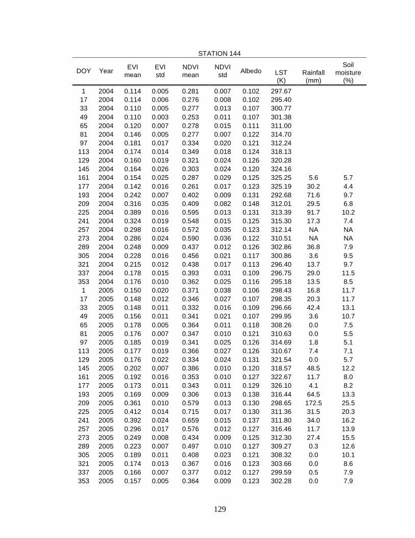
129

STATION 144

DOY Year EVI

mean EVI std

NDVI mean

NDVI std

Albedo LST (K)

Rainfall (mm)

Soil moisture

(%)

1 2004 0.114 0.005 0.281 0.007 0.102 297.67

17 2004 0.114 0.006 0.276 0.008 0.102 295.40

33 2004 0.110 0.005 0.277 0.013 0.107 300.77

49 2004 0.110 0.003 0.253 0.011 0.107 301.38

65 2004 0.120 0.007 0.278 0.015 0.111 311.00

81 2004 0.146 0.005 0.277 0.007 0.122 314.70

97 2004 0.181 0.017 0.334 0.020 0.121 312.24

113 2004 0.174 0.014 0.349 0.018 0.124 318.13

129 2004 0.160 0.019 0.321 0.024 0.126 320.28

145 2004 0.164 0.026 0.303 0.024 0.120 324.16

161 2004 0.154 0.025 0.287 0.029 0.125 325.25 5.6 5.7

177 2004 0.142 0.016 0.261 0.017 0.123 325.19 30.2 4.4

193 2004 0.242 0.007 0.402 0.009 0.131 292.68 71.6 9.7

209 2004 0.316 0.035 0.409 0.082 0.148 312.01 29.5 6.8

225 2004 0.389 0.016 0.595 0.013 0.131 313.39 91.7 10.2

241 2004 0.324 0.019 0.548 0.015 0.125 315.30 17.3 7.4

257 2004 0.298 0.016 0.572 0.035 0.123 312.14 NA NA

273 2004 0.286 0.024 0.590 0.036 0.122 310.51 NA NA

289 2004 0.248 0.009 0.437 0.012 0.126 302.86 36.8 7.9

305 2004 0.228 0.016 0.456 0.021 0.117 300.86 3.6 9.5

321 2004 0.215 0.012 0.438 0.017 0.113 296.40 13.7 9.7

337 2004 0.178 0.015 0.393 0.031 0.109 296.75 29.0 11.5

353 2004 0.176 0.010 0.362 0.025 0.116 295.18 13.5 8.5

1 2005 0.150 0.020 0.371 0.038 0.106 298.43 16.8 11.7

17 2005 0.148 0.012 0.346 0.027 0.107 298.35 20.3 11.7

33 2005 0.148 0.011 0.332 0.016 0.109 296.66 42.4 13.1

49 2005 0.156 0.011 0.341 0.021 0.107 299.95 3.6 10.7

65 2005 0.178 0.005 0.364 0.011 0.118 308.26 0.0 7.5

81 2005 0.176 0.007 0.347 0.010 0.121 310.63 0.0 5.5

97 2005 0.185 0.019 0.341 0.025 0.126 314.69 1.8 5.1

113 2005 0.177 0.019 0.366 0.027 0.126 310.67 7.4 7.1

129 2005 0.176 0.022 0.334 0.024 0.131 321.54 0.0 5.7

145 2005 0.202 0.007 0.386 0.010 0.120 318.57 48.5 12.2

161 2005 0.192 0.016 0.353 0.010 0.127 322.67 11.7 8.0

177 2005 0.173 0.011 0.343 0.011 0.129 326.10 4.1 8.2

193 2005 0.169 0.009 0.306 0.013 0.138 316.44 64.5 13.3

209 2005 0.361 0.010 0.579 0.013 0.130 298.65 172.5 25.5

225 2005 0.412 0.014 0.715 0.017 0.130 311.36 31.5 20.3

241 2005 0.392 0.024 0.659 0.015 0.137 311.80 34.0 16.2

257 2005 0.296 0.017 0.576 0.012 0.127 316.46 11.7 13.9

273 2005 0.249 0.008 0.434 0.009 0.125 312.30 27.4 15.5

289 2005 0.223 0.007 0.497 0.010 0.127 309.27 0.3 12.6

305 2005 0.189 0.011 0.408 0.023 0.121 308.32 0.0 10.1

321 2005 0.174 0.013 0.367 0.016 0.123 303.66 0.0 8.6

337 2005 0.166 0.007 0.377 0.012 0.127 299.59 0.5 7.9

353 2005 0.157 0.005 0.364 0.009 0.123 302.28 0.0 7.9

130

1 2006 0.149 0.005 0.332 0.006 0.125 303.52 0.5 7.7

17 2006 0.141 0.006 0.307 0.006 0.125 302.10 0.0 7.3

33 2006 0.134 0.003 0.306 0.008 0.120 306.01 9.9 8.7

49 2006 0.136 0.002 0.253 0.002 0.125 307.74 0.0 10.5

65 2006 0.120 0.002 0.264 0.007 0.128 308.09 7.6 8.9

81 2006 0.121 0.002 0.253 0.006 0.135 312.45 0.0 10.0

97 2006 0.136 0.006 0.224 0.007 0.136 320.15 0.0 9.1

113 2006 0.128 0.008 0.253 0.011 0.139 319.18 1.0 8.7

129 2006 0.127 0.007 0.243 0.009 0.136 324.27 0.0 9.0

145 2006 0.140 0.004 0.243 0.008 0.139 323.31 25.7 12.9

161 2006 0.143 0.007 0.275 0.011 0.132 326.11 14.2 15.1

177 2006 0.321 0.012 0.477 0.020 0.127 311.80 101.9 26.0

193 2006 0.342 0.021 0.643 0.028 0.131 318.38 NA NA

209 2006 0.421 0.017 0.652 0.016 0.136 290.65 17.8 12.4

225 2006 0.421 0.017 0.599 0.020 0.138 308.42 65.0 10.7

241 2006 0.420 0.012 0.648 0.019 0.133 306.66 101.6 16.5

257 2006 0.357 0.022 0.678 0.032 0.126 310.00 0.0 9.3

273 2006 0.252 0.006 0.422 0.005 0.139 310.86 0.0 7.3

289 2006 0.209 0.009 0.414 0.017 0.120 307.09

305 2006 0.197 0.009 0.432 0.012 0.118 306.77

321 2006 0.182 0.007 0.414 0.012 0.119 302.13

337 2006 0.163 0.007 0.355 0.012 0.121 299.29

353 2006 0.147 0.004 0.312 0.006 0.118 291.27

9 2007 0.135 0.007 0.292 0.011 0.117 297.85

25 2007 0.123 0.009 0.283 0.015 0.116 NA

33 2007 0.123 0.006 0.274 0.019 0.116 303.20

49 2007 0.119 0.006 0.242 0.011 0.122 303.63

65 2007 0.118 0.002 0.271 0.010 0.126 314.75

81 2007 0.149 0.016 0.316 0.027 0.125 311.44

97 2007 0.145 0.014 0.294 0.024 0.131 312.23

113 2007 0.149 0.019 0.306 0.022 0.132 317.03

129 2007 0.144 0.017 0.273 0.017 0.134 321.46

145 2007 0.139 0.017 0.280 0.027 0.134 323.09

161 2007 0.170 0.015 0.372 0.018 0.131 325.85

177 2007 0.366 0.027 0.581 0.031 0.134 330.18

193 2007 0.461 0.027 0.745 0.027 0.138 312.32

209 2007 0.404 0.010 0.657 0.009 0.146 308.18

225 2007 0.351 0.025 0.630 0.025 0.139 NA

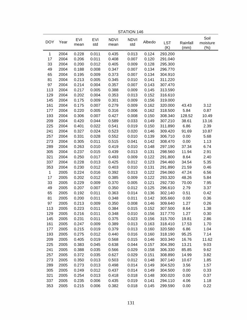
131

STATION 146

DOY Year EVI

mean EVI std

NDVI mean

NDVI std

Albedo LST (K)

Rainfall (mm)

Soil moisture

(%)

1 2004 0.228 0.011 0.435 0.013 0.124 293.200

17 2004 0.206 0.011 0.408 0.007 0.120 291.040

33 2004 0.200 0.012 0.405 0.009 0.128 295.300

49 2004 0.188 0.008 0.347 0.007 0.134 296.770

65 2004 0.195 0.009 0.373 0.007 0.134 304.910

81 2004 0.213 0.005 0.345 0.010 0.141 311.220

97 2004 0.214 0.004 0.357 0.007 0.143 307.470

113 2004 0.217 0.005 0.388 0.009 0.145 313.590

129 2004 0.202 0.004 0.353 0.013 0.152 316.610

145 2004 0.175 0.009 0.301 0.009 0.156 319.000

161 2004 0.175 0.007 0.279 0.009 0.162 320.000 43.43 3.12

177 2004 0.220 0.005 0.316 0.006 0.162 318.500 5.84 0.87

193 2004 0.306 0.007 0.427 0.008 0.150 308.340 128.52 10.49

209 2004 0.420 0.044 0.589 0.033 0.149 307.210 38.61 13.16

225 2004 0.401 0.022 0.541 0.019 0.150 311.890 6.86 2.39

241 2004 0.327 0.024 0.523 0.020 0.146 309.420 91.69 10.87

257 2004 0.331 0.028 0.552 0.010 0.139 306.710 0.00 5.68

273 2004 0.305 0.011 0.515 0.041 0.142 308.470 0.00 1.13

289 2004 0.263 0.010 0.419 0.010 0.148 297.190 37.34 6.74

305 2004 0.237 0.015 0.439 0.013 0.131 298.560 11.94 2.91

321 2004 0.250 0.017 0.493 0.009 0.122 291.800 8.64 2.40

337 2004 0.228 0.013 0.425 0.012 0.123 294.460 34.54 5.35

353 2004 0.230 0.012 0.403 0.010 0.131 291.890 21.59 0.46

1 2005 0.224 0.016 0.392 0.013 0.122 294.060 47.24 6.56

17 2005 0.202 0.012 0.385 0.009 0.122 293.320 48.26 5.84

33 2005 0.229 0.009 0.370 0.005 0.121 292.730 70.00 7.95

49 2005 0.207 0.007 0.350 0.012 0.125 296.610 2.79 3.37

65 2005 0.192 0.011 0.363 0.014 0.136 302.140 0.51 0.42

81 2005 0.200 0.011 0.348 0.011 0.142 305.660 0.00 0.36

97 2005 0.213 0.009 0.350 0.008 0.146 309.640 1.27 0.26

113 2005 0.223 0.011 0.384 0.015 0.152 307.500 8.64 1.38

129 2005 0.216 0.011 0.348 0.010 0.156 317.770 1.27 0.30

145 2005 0.231 0.011 0.375 0.023 0.156 315.700 19.81 2.86

161 2005 0.247 0.009 0.389 0.013 0.163 318.410 17.53 1.70

177 2005 0.215 0.019 0.379 0.013 0.160 320.580 6.86 1.04

193 2005 0.275 0.012 0.440 0.016 0.160 318.190 95.25 7.14

209 2005 0.405 0.019 0.568 0.015 0.146 303.340 16.76 11.62

225 2005 0.383 0.045 0.638 0.044 0.157 304.390 13.21 9.03

241 2005 0.388 0.035 0.566 0.029 0.158 306.330 85.85 9.62

257 2005 0.372 0.035 0.627 0.029 0.151 308.890 14.99 3.82

273 2005 0.350 0.013 0.503 0.012 0.148 307.140 10.67 1.85

289 2005 0.273 0.013 0.498 0.014 0.149 304.520 3.56 1.57

305 2005 0.249 0.012 0.437 0.014 0.149 304.500 0.00 0.33

321 2005 0.254 0.013 0.418 0.018 0.148 300.020 0.00 0.37

337 2005 0.235 0.006 0.435 0.019 0.141 294.110 4.06 1.18

353 2005 0.215 0.006 0.382 0.018 0.145 299.590 0.00 0.22

132

1 2006 0.208 0.005 0.379 0.014 0.149 299.320 0.00 0.51

17 2006 0.199 0.004 0.365 0.014 0.151 298.320 0.00 0.48

33 2006 0.189 0.005 0.339 0.011 0.154 301.450 1.78 0.53

49 2006 0.177 0.003 0.277 0.010 0.160 301.730 3.05 0.67

65 2006 0.167 0.001 0.290 0.008 0.169 302.270 3.81 2.69

81 2006 0.165 0.003 0.280 0.007 0.168 306.560 0.00 0.46

97 2006 0.154 0.009 0.259 0.008 0.168 313.140 0.00 0.57

113 2006 0.165 0.007 0.243 0.008 0.178 314.710 0.25 0.65

129 2006 0.149 0.004 0.243 0.006 0.179 320.130 0.00 0.72

145 2006 0.153 0.004 0.244 0.008 0.180 318.620 6.35 1.91

161 2006 0.161 0.003 0.250 0.007 0.183 322.350 6.86 2.03

177 2006 0.175 0.006 0.267 0.008 0.164 314.880 134.11 12.80

193 2006 0.414 0.014 0.564 0.018 0.164 308.790 292.10 17.20

209 2006 0.505 0.036 0.695 0.029 0.162 287.540 NA NA

225 2006 0.511 0.042 0.711 0.031 0.158 300.900 NA NA

241 2006 0.548 0.034 0.778 0.020 0.142 300.640 97.79 21.52

257 2006 0.489 0.016 0.678 0.012 0.147 302.700 0.25 4.74

273 2006 0.356 0.014 0.615 0.010 0.140 304.530 0.00 1.50

289 2006 0.290 0.015 0.539 0.018 0.134 301.840

305 2006 0.296 0.025 0.542 0.017 0.131 301.060

321 2006 0.274 0.019 0.534 0.008 0.131 298.110

337 2006 0.266 0.014 0.526 0.012 0.135 294.750

353 2006 0.240 0.021 0.457 0.009 0.134 290.890

9 2007 0.246 0.007 0.412 0.007 0.151 293.270

25 2007 0.199 0.004 0.384 0.018 0.141 NA

33 2007 0.205 0.007 0.363 0.008 0.142 297.510

49 2007 0.188 0.004 0.335 0.013 0.149 299.710

65 2007 0.196 0.008 0.339 0.009 0.154 310.310

81 2007 0.193 0.003 0.339 0.009 0.150 307.140

97 2007 0.191 0.008 0.314 0.012 0.154 308.250

113 2007 0.195 0.004 0.312 0.010 0.155 312.510

129 2007 0.176 0.008 0.275 0.018 0.160 317.780

145 2007 0.183 0.006 0.274 0.011 0.169 319.210

161 2007 0.176 0.008 0.326 0.014 0.172 321.980

177 2007 0.321 0.013 0.570 0.019 0.169 323.650

193 2007 0.404 0.025 0.656 0.022 NA 311.210

209 2007 0.407 0.018 0.630 0.031 0.136 305.380

225 2007 0.386 0.026 0.638 0.021 0.148 NA

133

STATION 147

DOY Year EVI

mean EVI

stdev NDVI mean

NDVI stdev

Albedo LST (K)

Rainfall (mm)

Soil moisture

(%)

1 2004 0.144 0.005 0.270 0.008 0.156 301.470

17 2004 0.136 0.007 0.247 0.006 0.150 296.560

33 2004 0.128 0.003 0.245 0.005 0.154 301.820

49 2004 0.118 0.004 0.222 0.004 0.168 301.230

65 2004 0.131 0.003 0.238 0.004 0.154 311.270

81 2004 0.152 0.004 0.244 0.006 0.160 313.140

97 2004 0.156 0.007 0.256 0.006 0.157 314.270

113 2004 0.146 0.006 0.251 0.007 0.160 319.660

129 2004 0.128 0.005 0.223 0.007 0.164 321.580

145 2004 0.122 0.007 0.205 0.004 0.159 324.200

161 2004 0.120 0.004 0.199 0.005 0.167 325.230

177 2004 0.121 0.003 0.192 0.004 0.160 328.070

193 2004 0.338 0.063 0.459 0.100 0.183 NA

209 2004 0.348 0.013 0.536 0.020 0.176 309.770 69.6 8.4

225 2004 0.339 0.007 0.483 0.011 0.159 315.400 12.7 4.2

241 2004 0.306 0.013 0.531 0.023 0.168 315.200 40.9 6.9

257 2004 0.232 0.005 0.394 0.013 0.157 314.780 14.2 4.5

273 2004 0.199 0.006 0.334 0.006 0.161 314.950 0.0 1.1

289 2004 0.165 0.004 0.302 0.007 0.171 306.910 30.5 5.4

305 2004 0.172 0.003 0.312 0.006 0.150 305.190 2.3 3.2

321 2004 0.164 0.006 0.321 0.004 0.151 297.720 4.8 4.0

337 2004 0.170 0.007 0.305 0.006 0.147 300.200 31.0 7.6

353 2004 0.167 0.004 0.301 0.006 0.156 296.700 15.5 2.6

1 2005 0.165 0.004 0.297 0.006 0.150 297.640 34.0 9.1

17 2005 0.172 0.006 0.360 0.009 0.145 298.810 27.7 7.8

33 2005 0.175 0.008 0.326 0.011 0.146 294.200 66.3 11.3

49 2005 0.188 0.009 0.318 0.012 0.154 300.260 2.8 6.1

65 2005 0.198 0.013 0.342 0.014 0.151 305.580 9.7 4.0

81 2005 0.191 0.007 0.320 0.008 0.155 310.640 0.0 1.5

97 2005 0.175 0.006 0.282 0.006 0.162 315.730 0.0 0.8

113 2005 0.158 0.011 0.272 0.007 0.157 315.450 8.6 2.0

129 2005 0.138 0.005 0.245 0.005 0.162 321.460 0.0 0.9

145 2005 0.136 0.004 0.234 0.005 0.158 319.800 14.2 4.0

161 2005 0.133 0.002 0.235 0.002 0.163 323.410 6.1 1.6

177 2005 0.142 0.003 0.219 0.005 0.164 327.380 0.5 1.0

193 2005 0.174 0.030 0.279 0.047 0.194 319.970 79.0 5.1

209 2005 0.414 0.021 0.661 0.019 0.176 NA 135.4 7.3

225 2005 0.377 0.016 0.616 0.022 0.163 309.900 6.6 0.9

241 2005 0.279 0.010 0.457 0.016 0.151 315.320 13.2 0.8

257 2005 0.208 0.005 0.380 0.010 0.158 317.490 0.5 0.3

273 2005 0.189 0.010 0.316 0.008 0.159 314.900 13.0 2.0

289 2005 0.178 0.013 0.300 0.006 0.162 311.650 0.3 1.4

305 2005 0.158 0.006 0.267 0.006 0.168 310.470 0.0 0.2

321 2005 0.155 0.004 0.259 0.007 0.165 306.000 0.0 0.1

337 2005 0.141 0.007 0.260 0.005 0.175 301.010 2.3 0.2

353 2005 0.132 0.003 0.239 0.005 0.166 304.740 0.0 0.1

134

1 2006 0.123 0.004 0.234 0.006 0.170 305.780 0.0 0.0

17 2006 0.123 0.004 0.229 0.005 0.174 304.160 0.0 0.1

33 2006 0.115 0.002 0.215 0.002 0.170 309.280 0.0 0.1

49 2006 0.122 0.003 0.201 0.004 0.169 310.340 1.5 0.2

65 2006 0.122 0.002 0.208 0.003 0.177 309.690 3.3 0.2

81 2006 0.115 0.001 0.205 0.002 0.175 313.840 0.0 0.3

97 2006 0.112 0.003 0.195 0.002 0.179 319.910 0.0 0.4

113 2006 0.127 0.002 0.191 0.003 0.180 320.250 0.0 0.5

129 2006 0.110 0.001 0.189 0.001 0.178 323.860 0.0 0.6

145 2006 0.121 0.002 0.191 0.003 0.181 324.410 1.8 0.7

161 2006 0.113 0.002 0.196 0.003 0.179 328.670 19.8 1.5

177 2006 0.177 0.016 0.285 0.013 0.175 315.460 110.7 10.4

193 2006 0.336 0.008 0.492 0.023 0.159 318.430 51.6 6.9

209 2006 0.448 0.010 0.618 0.014 0.158 306.570 179.6 9.5

225 2006 0.444 0.017 0.611 0.024 0.161 307.640 72.6 7.7

241 2006 0.439 0.021 0.665 0.025 0.156 306.240 78.7 9.4

257 2006 0.397 0.011 0.581 0.014 0.153 309.190 0.3 3.6

273 2006 0.300 0.008 0.521 0.014 0.159 312.060

289 2006 0.229 0.005 0.414 0.011 0.153 307.720

305 2006 0.238 0.007 0.419 0.008 0.149 307.970

321 2006 0.203 0.004 0.384 0.010 0.154 304.230

337 2006 0.178 0.010 0.329 0.012 0.158 300.730

353 2006 0.165 0.005 0.296 0.005 0.160 298.000

9 2007 0.146 0.007 0.266 0.004 0.149 299.780

25 2007 0.135 0.005 0.260 0.010 0.148 NA

33 2007 0.145 0.002 0.248 0.004 0.155 305.210

49 2007 0.140 0.002 0.237 0.004 0.152 306.120

65 2007 0.124 0.002 0.217 0.004 0.156 315.280

81 2007 0.123 0.005 0.219 0.008 0.157 314.110

97 2007 0.125 0.004 0.207 0.008 0.159 314.690

113 2007 0.126 0.007 0.197 0.007 0.160 319.280

129 2007 0.122 0.006 0.190 0.009 0.162 323.080

145 2007 0.115 0.004 0.189 0.007 0.163 324.250

161 2007 0.117 0.004 0.203 0.005 0.161 327.340

177 2007 0.138 0.004 0.196 0.006 0.177 328.450

193 2007 0.361 0.014 0.527 0.017 0.139 NA

209 2007 0.372 0.008 0.520 0.011 0.146 309.830

225 2007 0.347 0.008 0.545 0.011 0.147 NA

135

APPENDIX 2

GLOSSARY OF TERMS

ANNP: Aboveground Net Primary Production.

BMA: Backward Moving Average.

BRDF: bidirectional Reflectance Distribution Function.

CAPE: Convective Available Energy.

ENSO: El Niño Southern Oscillation.

EVI: Enhanced Vegetation Index.

FG: Functional group.

FMA: Forward Moving Average

GPR: Greenness Precipitation Ratio.

HDF: Hierarchical Data Format.

iNDVI: Time integrated Normalized Difference Vegetation Index.

ITCZ: Inter-tropical Convergence Zone.

LST: Land Surface Temperature.

MODIS: Moderate Resolution Imaging Spectroradiometer.

MVC: Maximum Value Composite.

NAM: North American Monsoon.

NDVI: Normalized Difference Vegetation Index.

NPP: Net Primary Production.

RMSE : Root Mean Square Error of the Difference.

RUE: Rain Use Efficiency.

SST: Sea Surface Temperature.

136

APPENDIX 3

MATLAB SCRIPTS

The following MATLAB™ script was used to estimate the Forward Moving

Average (FMA) and the Backward Moving Average (BMA) in the original EVI time

series. Theses two lagged time series are used to estimate the staring and ending point of

vegetation activity.

clear; close all; load stat130.txt x= [stat130(:,1)]; y= [stat130(:,2)]; plot(x,y,'.-k'); hold on; sm = smooth(y,'sgolay',3); plot (x,sm,'LineWidth',2); xlabel('Days'); ylabel('EVI'); title('EVI Time Series for Station 130') hold on; [xxl,yyl]=getmoving(x,y,3,0); [xxr,yyr]=getmoving(x,y,3,1); plot(xxl,yyl,'-r',xxr,yyr,'-g'); xyarray=[x y] smarray=[x y] legend('original data','FMA','BMA') hold off

The “getmoving” function is defined with the following MATLAB™ script.

function[xa,ya]=getmoving(x,y,w,dir) %if dir =1 it will do it to the right, if dir =0 the it will do it to the %left if (dir==1) ya= 1:(length(x)-(w-1)); xa= 1:(length(x)-(w-1)); for (i=1:(length(x)-(w-1))) ya(i)=mean(y(i:i+w-1)); xa(i)=x(i); end else ya= 1:(length(x)-(w-1)); xa= 1:(length(x)-(w-1)); for (i=w:length(x)) ya(i-(w-1))=mean(y(i-(w-1):i)); xa(i-(w-1))=x(i);

137

end end

Once the starting and ending point of vegetation activity are established, we use

the 16-time periods as input to calculate the vegetation metrics for the different years

used in the analysis. In this case, we used the station 130 as an example.

clear; close all; load stat130.txt x= [stat130(:,1)]; y= [stat130(:,2)]; plot(x,y,'.-k'); hold on; sm = smooth(y,'sgolay',3) plot (x,sm,'LineWidth',2); xlabel('Days'); ylabel('EVI'); title('EVI Time Series for Station 130') hold on; xyarray=[x y] smarray=[x sm] figure(2)%Figure for vegetation metrics for year 2004 t= y(12:25); u= x(12:25); plot(u,t,'-g'); area_04=trapz(u,t) evimax_04=max(t) evimin_04=min(t) RtUp_04=(evimax_04-xyarray(12,2))/(xyarray(14,1)-xyarray(12,1)) RtDn_04=(xyarray(25,2)-evimax_04)/(xyarray(25,1)- xyarray(14,1)) RanVeg_04=evimax_04-evimin_04 Durgreen_04= xyarray(25,1)-xyarray(12,1) Timemax_04= xyarray(14,1)- xyarray(12,1) figure(3)%figure for vegetation metrics for year 2005 tt= y(34:51); uu= x(34:51); plot(uu,tt,'-g'); area_05=trapz(uu,tt) evimax_05=max(tt) evimin_05=min(tt) RtUp_05=(evimax_05-xyarray(34,2))/(xyarray(37,1)-xyarray(34,1)) RtDn_05=(xyarray(51,2)-evimax_05)/(xyarray(51,1)- xyarray(37,1)) RanVeg_05= evimax_05-evimin_05 Durgreen_05= xyarray(51,1)-xyarray(34,1) Timemax_05= xyarray(37,1)- xyarray(34,1) figure (4)%figure for vegetation metrics for year 2006 ttt= y(56:71); uuu= x(56:71); plot(uuu,ttt,'-g');

138

area_06=trapz(uuu,ttt) evimax_06=max(ttt) evimin_06=min(ttt) RtUp_06=(evimax_06-xyarray(56,2))/(xyarray(60,1)-xyarray(56,1)) RtDn_06=(xyarray(71,2)-evimax_06)/(xyarray(71,1)- xyarray(60,1)) RanVeg_06=evimax_06-evimin_06 Durgreen_06= xyarray(71,1)-xyarray(56,1) Timemax_06= xyarray(60,1)- xyarray(56,1)