LTE Multicodeword-MIMO: Hybrid-ARQ Perfomance …lib.tkk.fi/Dipl/2010/urn100398.pdf · LTE...

Aalto Universtiy

School of Science and Technology

Faculty of Information and Natural Sciences

Degree programme of Communication Engineering

Tomasz Burzanowski

LTE Multicodeword-MIMO:Hybrid-ARQ Perfomance Studies

Master's Thesis

Espoo, December 3, 2010

Supervisor: Professor Olav Tirkkonen, Aalto University

Instructor: Professor Olav Tirkkonen, Aalto University

Aalto UniversitySchool of Science and Technology ABSTRACT OFFaculty of Information and Natural Sciences MASTER'S THESISDegree Programme of Communication Engineering

Author: Tomasz BurzanowskiTitle of thesis:LTE Multicodeword-MIMO: Hybrid-ARQ Perfomance Studies

Date: December 3, 2010 Pages: 10 + 80Professorship: Data Communications Software Code: S-114-2Supervisor: Professor Olav TirkkonenInstructor: Professor Olav Tirkkonen

Mobile communication is going through major changes since the intro-duction of �rst generation mobile phones. Not only phones, but varioushandheld devices are starting to use the mobile communication networkfor internet browsing, multimedia or even online gaming. There is a highneed for fast mobile connection and therefore new standards and speci�-cations need to be created to satisfy the consumer requirements.

Long Term Evolution (LTE) is the latest candidate for the next mobilecommunication standard led by Third Generation Partnership Project(3GPP). LTEs main features are high throughput, low latency, simplearchitecture and low operating costs.

Since mobile data transmission is a non linear process, a simulator isbuilt to model the procedure. Simulator made for this thesis was writtenin MATLAB meeting the 3GPPs set standards for LTE. Three di�erentMultiple Input Multiple Output (MIMO) downlink HARQ scenarios werecreated and their performance was evaluated.The main focus of this thesisis the performance comparison of the three downlink scenarios; howeverthe veri�cation of the simulator model plays also a signi�cant role in thiswork.

Keywords: LTE, MIMO, HARQ, Throughput, Blanking, Non-blanking,Link adaptation, LTE downlink simulator

Language: English

ii

Aalto-yliopistoTeknillinen korkeakoulu DIPLOMITYÖNInformaatio- ja luonnontiedeiden tiedekunta TIIVISTELMÄTietoliikennetekniikan koulutusohjelma

Tekijä: Tomasz BurzanowskiTyön nimi:LTE Multicodeword-MIMO: Hybrid-ARQ Perfomance Studies

Päiväys: 3. joulukuuta 2010 Sivumäärä: 10 + 80Professuuri: Tietoliikennetekniikka Koodi: S-114-2Työn valvoja: Professori Olav TirkkonenTyön ohjaaja: Professori Olav Tirkkonen

Langattomassa tiedonsiirrossa on tällä hetkellä meneillään suuria muu-toksia, sitten ensimmäisen matkapuhelinsukupolven käyttöönoton. Uu-sia datapuhelimia, kuten myös kämmentietokoneita käytetään internetinselaamiseen, videoiden katselemiseen ja pelaamiseen matkapuhelinverkonkautta. Voidaakseen tyydyttämään kuluttajien vaatimukset, tarve uusienlangattoman tiedonsiirron normien luomiseen on merkittävä.

Long Term Evolution (LTE) on, Third Generation Partership Project:in(3GPP) johtama, ehdokas seuraavaksi matkapuhelinsukupolven standard-iksi. LTE:n ominaisuuksiin kuuluvat mm. korkea suoritusteho, matalalatenssi, yksinkertaisuus ja alhaiset kustannukset. Tulevassa standardissaon aihealueita, joita ei ole varsinaisesti tutkittu akateemisessa maailmassakuten Hybrid Automatic Repeat Request:in (HARQ) suorituskykyä.

Koska langaton tiedonsiirto on epälineaarinen prosessi, sitä mallinnetaansimulaattorin avulla. Simulaattori on tehty MATLAB ympäristössäLTE:n standardien mukaisesti. Kolme eri Multiple Input Multiple Out-put (MIMO) downlink HARQ skenaariota luotiin ja niiden suorituskykyäarvioitiin. Pääpaino työn tutkimukselle kohdistuu kolmen HARQ:n suori-tuskykyyn, tosin simulaattorimallin todistaminen on myös keskeinen osatätä työtä.

Avainsanat: LTE, MIMO, HARQ, suorituskyky, Blanking, Non-blanking,linkki adaptaatio, LTE simulaattori

Kieli: englanti

iii

Acknowledgements

I would like to express my sincere gratitude to my supervisor Prof. Olav Tirkko-nen and MSc. Kalle Ruttik for their support and guidance and patience duringthe course of this work. Their encouragement and support has always been asource of motivation for me to explore various aspects of the topic. Discussionswith them have always been instructive and insightful and helped me to identifymy ideas.

Finally, I am very grateful to my parents Halina and Aleksy and my youngerbrother Adam Burzanowski for their sacri�ces, unremitting motivation, love andtheir continuous support during my stay at Aalto University School of Scienceand Technology in Otaniemi.

Espoo December 3, 2010

Tomasz Burzanowski

iv

Abbreviations and Acronyms

3G 3rd Generation3GPP 3rd Generation Partnership ProjectACK Postive AcknowledgementAMC Adaptive Modulation and CodingARQ Automatic Repeat RequestAWGN Additive White Gaussian NoiseBER Bit Error RateBLER Block Error RateBPSK Binary Phase Shift KeyingCDD Cyclic Delay DiversityCIR Channel Impulse ResponseCP Cyclic Pre�xCQI Channel Quality IndicatorCRC Cyclic Redundancy CheckdB DecibelDFT Discrete Fourier TransformDRX Discontinuous ReceptionDVB Digital Video BroadcastingDwPTS Downlink Pilot TimeslotE-UTRAN Evolved-UMTS Terrestial Radio Access NetworkeNodeB Evolved Node Base StationFDD Frequency Division MultiplexingFEC Forward Error CorrectionFFT Fast Fourier TransformGB Giga ByteGHz Giga HertzGP Guard PeriodGUI Graphical User InterfaceHARQ Hybrid Automatic Repeat RequestHz HertzICI Intercarrier interferenceIDFT Inverse Discrete Fourier Transform

vi

IFFT Inverse Fast Fourirer TransformITU International Telecommunication UnionISI Intersymbolic interferenceLMS Least Minimum SquareLS Least SquareLTE Long Term EvolutionMAC Medium Access ControlMCS Modulation and Coding SchemeMIMO Multiple Input Multiple OutputMMSE Minimum Mean SquareNACK Negatice AcknowledgementNDI New Data IndicatorOFDM Orthogonal Frequency Division MultiplexingPAPR Peak-to-Average Power RatioPCCC Parallel Concatenated Convolutional CodePDCP Packet Data Convergence ProtocolPDU Protocol Data UnitQAM Quadrature Amplitude modulationQoS Quality of ServiceQPSK Quadrature Phase Shift KeyingRAN Radio Access NetworkRB Resource BlockRE Resource ElementRLC Radio Link ControlRTT Round Trip TimeRV Redundancy VersionSAP Service Access PointSB SubblockSDU Service Data UnitTDD Time Division MultiplexingTKK Teknillinen KorkeakouluTTI Transmission Time IntervallUE User EquipmentUMTS Universal Mobile Telecommunication SystemUpPTS Uplink Pilot TimeslotVLSI Very-large-scale integrationWCDMA Wideband Code Divison Multiple AccessWiMax Worldwide Interoperability for Microwave Access

vii

Contents

1 Introduction 1

1.1 Background . . . . . . . . . . . . . . . . . . . . . . . . . . . . . . 1

1.2 Motivation and problem statement . . . . . . . . . . . . . . . . . 2

1.3 Outline . . . . . . . . . . . . . . . . . . . . . . . . . . . . . . . . . 3

2 OFDM Principle 4

2.1 Multicarrier-modulation . . . . . . . . . . . . . . . . . . . . . . . 4

2.2 Orthogonal frequency division multiplexing . . . . . . . . . . . . . 6

2.3 Model . . . . . . . . . . . . . . . . . . . . . . . . . . . . . . . . . 11

3 Background 13

3.1 LTE standardization . . . . . . . . . . . . . . . . . . . . . . . . . 13

3.2 LTE key features and requirements . . . . . . . . . . . . . . . . . 15

3.3 LTE frame structure . . . . . . . . . . . . . . . . . . . . . . . . . 16

3.3.1 Type 1 (FDD) and Type 2 (TDD) . . . . . . . . . . . . . 17

3.3.2 Slot structure . . . . . . . . . . . . . . . . . . . . . . . . . 18

3.3.3 Cyclic pre�x . . . . . . . . . . . . . . . . . . . . . . . . . . 20

3.4 Modulation . . . . . . . . . . . . . . . . . . . . . . . . . . . . . . 20

3.4.1 QPSK, 16-QAM and 64-QAM . . . . . . . . . . . . . . . . 21

3.4.2 Pilot structure . . . . . . . . . . . . . . . . . . . . . . . . 25

3.4.3 Channel estimation . . . . . . . . . . . . . . . . . . . . . . 26

3.5 Link adaptation . . . . . . . . . . . . . . . . . . . . . . . . . . . . 27

3.5.1 Adaptive Modulation and Coding . . . . . . . . . . . . . . 28

viii

CONTENTS

3.6 MIMO . . . . . . . . . . . . . . . . . . . . . . . . . . . . . . . . . 29

3.6.1 Basics . . . . . . . . . . . . . . . . . . . . . . . . . . . . . 30

3.6.2 Spatial multiplexing . . . . . . . . . . . . . . . . . . . . . 30

3.6.3 Pre-coding . . . . . . . . . . . . . . . . . . . . . . . . . . . 31

3.6.4 Transmit diversity . . . . . . . . . . . . . . . . . . . . . . 33

3.7 Multicodeword-MIMO HARQ . . . . . . . . . . . . . . . . . . . . 34

3.7.1 ARQ protocol categories . . . . . . . . . . . . . . . . . . . 34

3.7.2 Chase Combining and Incremental Redundancy . . . . . . 38

3.7.3 Multicodeword-MIMO HARQ alternatives . . . . . . . . . 39

3.7.3.1 Independent . . . . . . . . . . . . . . . . . . . . . 40

3.7.3.2 Blanking . . . . . . . . . . . . . . . . . . . . . . 40

3.7.3.3 Non-blanking . . . . . . . . . . . . . . . . . . . . 40

4 LTE Downlink 42

4.1 RLC Layer . . . . . . . . . . . . . . . . . . . . . . . . . . . . . . . 42

4.2 MAC Layer . . . . . . . . . . . . . . . . . . . . . . . . . . . . . . 44

4.2.1 Multiplexing and mapping . . . . . . . . . . . . . . . . . . 44

4.2.2 Scheduling . . . . . . . . . . . . . . . . . . . . . . . . . . . 45

4.2.3 Discontinuous Reception (DRX) . . . . . . . . . . . . . . . 47

4.2.4 HARQ . . . . . . . . . . . . . . . . . . . . . . . . . . . . . 47

4.3 PHY Layer . . . . . . . . . . . . . . . . . . . . . . . . . . . . . . 47

4.3.1 Channel coding . . . . . . . . . . . . . . . . . . . . . . . . 48

4.3.1.1 CRC . . . . . . . . . . . . . . . . . . . . . . . . . 48

4.3.1.2 Turbo coding . . . . . . . . . . . . . . . . . . . . 49

4.3.2 Modulation . . . . . . . . . . . . . . . . . . . . . . . . . . 50

4.3.3 HARQ . . . . . . . . . . . . . . . . . . . . . . . . . . . . . 51

5 Simulator 53

5.1 System model . . . . . . . . . . . . . . . . . . . . . . . . . . . . . 53

5.1.1 Transmitter . . . . . . . . . . . . . . . . . . . . . . . . . . 55

5.1.2 Channel . . . . . . . . . . . . . . . . . . . . . . . . . . . . 55

ix

CONTENTS

5.1.2.1 Winner II model . . . . . . . . . . . . . . . . . . 56

5.1.2.2 Typical Urban model . . . . . . . . . . . . . . . . 56

5.1.3 Receiver . . . . . . . . . . . . . . . . . . . . . . . . . . . . 57

5.1.4 Simulator veri�cation . . . . . . . . . . . . . . . . . . . . . 58

5.1.4.1 BER QPSK . . . . . . . . . . . . . . . . . . . . . 59

5.1.4.2 BER 16-QAM . . . . . . . . . . . . . . . . . . . . 59

5.1.4.3 BER 64-QAM . . . . . . . . . . . . . . . . . . . . 60

5.1.4.4 HARQ functionality . . . . . . . . . . . . . . . . 62

5.1.4.5 Transmit diversity . . . . . . . . . . . . . . . . . 66

5.1.4.6 Link adaptation . . . . . . . . . . . . . . . . . . 67

5.1.4.7 MIMO transmission . . . . . . . . . . . . . . . . 67

6 Multicodeword-MIMO Performance 71

6.1 Simulation Results . . . . . . . . . . . . . . . . . . . . . . . . . . 71

6.2 Comparison . . . . . . . . . . . . . . . . . . . . . . . . . . . . . . 73

7 Conclusion 75

7.1 Future work . . . . . . . . . . . . . . . . . . . . . . . . . . . . . . 76

References 77

x

Chapter 1

Introduction

As introduction some background information with estimation of upcoming trendsin mobile communications is given. Next motivation and problem statement forwriting this thesis are described, followed by an outline of the remaining docu-ment.

1.1 Background

Due the increasing demand for higher data rates for wireless communication sys-tems and the growth of mobile data transfer usage, the wireless communicationarea has gained signi�cant attraction for mobile researches and industries world-wide. Mobile broadband is becoming reality and according to [23] out of theestimated 1.8 billion people, who will have broadband by 2012, some two thirdwill be mobile broadband customers and the majority will be served by HSPA(High Speed Packet Access) and LTE (Long Term Evolution).

The third Generation Partnership Project (3GPP) organization has started aninternational collaboration project to improve the Universal Mobile Telecommu-nication System (UMTS) and this also can be considered as a milestone towardsfourth generation (4G) standardization. The main focus of this project is to es-tablish a mobile broadband that will support the future demand of mobile userslike e�ciency improvement, service enhancement, lower maintenance and usagecosts and better integration with other standards. Table 1.1 describes the 3GPPgroup technical speci�cations [8].

High wireless communication quality and increasing data rates are limited throughbandwidth resources. Therefore rapidly growing number of users sharing the sameresource, more advanced technologies are needed to achieve satisfying spectral ef-

1

1.2 Motivation and problem statement 2

Release Speci�cation Date

Release 99 UMTS 3G networks, CDMA air interface March 2000Release 4 All-IP Core Network March 2001Release 5 IMS and HSDPA March - June 2002Release 6 WLAN, HSUPA and MBMS Dec. 2004 - March 2005Release 7 HSPA+ and EDGE Evolution. Dec. 2007Release 8 LTE December 2008Release 9 WiMax and LTE/UMTS Interoperability Dec. 2009Release 10 LTE Advanced March 2011?

Table 1.1: Technical speci�cation published by 3GPP

�ciency. Technologies like Orthogonal Frequency Division Multiplexing (OFDM)and multiple input, multiple output (MIMO), can improve the performance ofcurrent wireless communication systems. For future mobile communications sys-tem LTE is the next step and basis for future enhancements. LTE is the �rstcellular communication system optimized to support packet-switched data ser-vices, where packetized voice communication is just one part of it.

1.2 Motivation and problem statement

Since sending mobile data over certain channel is a highly non linear process,there is a need building a tool in form of a simulator to gain access to di�erentsubjects related with mobile communication as bit error rates (BER), channelestimation and throughput calculations.

The main focus of this thesis is to build a LTE downlink simulator using anolder generation simulator as a reference and to explore di�erent HARQ imple-mentation methods, which were discussed in [3] in 2006, but which are very littleexamined in the academic world. In 2010, for LTE-Advanced the discussion recon-sidering HARQ process bundling for multicodeword-MIMO to boost the spectrale�ciency and trying to keep the feedback overhead low [25]. The simulator hasbeen developed by TKK Communication Engineering Department in MATLABcoding environment and a long term goal is to have a clean structured tool fordemoing purposes at the Helsinki University of Technology. By structured ismeant, that di�erent functions from di�erent layers e.g. Physical (PHY) layer orMedium Access Control (MAC) layer are separated according to the standardsset by 3GPP.

1.3 Outline 3

This thesis investigates some of LTEs downlink physical layer algorithms, theirperformance and comparison in data throughput. Hybrid Automatic RepeatreQuest (HARQ) is described in the Chapter 3.7. There are three di�erent sim-ulation cases where the throughput is calculated for each case and each signal-to-interference-noise ratio (SINR). The following HARQ process scenarios areinvestigated in this paper:

• Two codewords and two independent HARQ processes

• Two codewords and one independent HARQ process

� Blanking

� Non-blanking

Where the second case is divided into two sub cases, blanking and non-blanking.Detailed description of the simulation scenarios is found in Chapter 3.7.

1.3 Outline

Chapter 2 describes the principle of OFDM transmission used in LTE standard,including multicarrier modulation and frequency division multiplexing. At theend of this chapter a mathematical model of an OFDM transceiver is shown andexplained.

In Chapter 3, the LTE standard is described beginning with a general standardiza-tion process followed by key features of LTE. Furthermore more detailed view ofLTE is given by introducing di�erent frame structures, modulation, link adapta-tion and multi antenna transmission as well as three di�erent HARQ procedures.

Chapter 4 is devoted to more detailed view of LTE downlink transmission, wherethe functionalities of the di�erent layers are introduced and explained.

In Chapter 5 the model used in the simulator built for this thesis is described indetails, including the veri�cation tests to prove it working in correct way.

In Chapter 6 three di�erent HARQ methods are investigated including simulationparameters and received graphical results.

In last Chapter 7 the conclusions from the simulation are listed and future worktopics are suggested.

Chapter 2

OFDM Principle

This chapter describes the principle of Orthogonal Frequency Division Multiplex-ing (OFDM). In the �rst section, a general introduction to multicarrier modula-tion including mathematic descriptions and illustrations is given.

Next. a more detailed view of OFDM including basic characteristics and relationbetween time and frequency domain is given. Also concept of cyclic pre�x withOFDM is introduced and how it is to be implemented in the LTE standard.

Finally a mathematic model of an OFDM transceiver including transmitter, re-ceiver and a simple one tap equalizer is illustrated.

2.1 Multicarrier-modulation

Multicarrier-modulation was �rst introduced in the 50's, but completed in the60's and forms the basis of the OFDM modulation principle. In this technique,the available bandwidthW is divided into number of Nc sub bands or sub carriers,where each of them has the width of ∆f = W

Nc. This is illustrated in Figure 2.1.

Instead of transmitting the data symbols serially, the multi-carrier transmitterdivides the symbols into blocks of Nc data symbols which are transmitted inparallel by modulating each sub carrier. Therefore the symbol duration for amodulated carrier is Tu = 1

W[21].

The multi-carrier signal can be described as a set of modulated carriers [22]:

s(t) =Nc−1∑k=0

xkΨk(t) (2.1)

4

2.1 Multicarrier-modulation 5

Figure 2.1: Division of bandwidth into Nc sub carriers

where

xk is the data symbol modulating the kth sub-carrier

Ψk(t) is the modulation waveform at the kth sub-carrier

s(t) is the multi-carrier modulated signal

Figure 2.2 illustrates the process of generating a multi-carrier modulated signal.To tone down the e�ects of fading when designing a multi-carrier system thefollowing steps can be taken into account [15].

• The data symbol duration can be made longer than the maximum excessdelay of the channel in time domain Tu >> τmax.

• The bandwidth of the sub carriers can be made small compared to thecoherence bandwidth of the channel in frequency domain Bcoh = W

Nc. The

sub bands now experience �at fading so the equalization can be reduced toa single complex multiplication per carrier.

It is to be noted, that these steps are adressing the same subject viewed fromdi�erent angle. The �rst looks at the problem from time domain point of viewand the second step can be taking into account in the frequency domain.

2.2 Orthogonal frequency division multiplexing 6

Figure 2.2: Principle of multi-carrier modulation

2.2 Orthogonal frequency division multiplexing

OFDM is a digital modulation method where the signal is divided into severalnarrow band channels at di�erent frequencies where modulation and multiplex-ing are combined. The technique was used in the 60's in several high frequencymilitary systems for parallel data transmission. OFDM become more popularwhen in 1966, Chang [49] patented the structure of it and published a conceptof using orthogonal overlapping multi tone signals for data communication. In1971, Weinstein and Ebert [29] �rst introduced Discrete Fourier Transform (DFT)to parallel data transmission system which become part of the modulation anddemodulation process. In the 90's OFDM, gained popularity in wide band datacommunications and today's improvements in very-large-scale integration (VLSI)technology allows fast and cost e�ective Fast Fourier Transform (FFT) implemen-tation of OFDM systems. It is used as a downlink transmission scheme for LTEand it also used for other radio technologies like WiMax and and Digital VideoBroadcasting (DVB).

OFDM transmission can be seen as a kind of multi-carrier transmission, never-theless some of its basics characteristics which di�er from basic multi-carrier of amore narrowband transmission are [21]:

• The use of large number of narrowband subcarriers comparing e.g. to LTE'spredecessor Wideband Code Division Multiple Access (WCDMA) where 20MHz bandwidth would be divided into four 5 MHz subcarriers. In com-parison, in OFDM transmission there can be several hundred subcarriers


carrying the data to the same receiver.

• Simple rectangular pulse shaping which corresponds to sinc-square shapedper subcarrier spectrum as illustrated in Figure 2.3

• Tight frequency domain subcarrier packing with subcarrier spacing ∆f =1Tu, where Tu is per subcarrier modulation symbol time as seen in Figure 2.4

Figure 2.3: (a) subcarrier pulse shape in time and (b) spectrum in frequncydomain

Figure 2.4: OFDM subcarrier spacing


The subcarrier pulses are chosen to be rectangular hence the task of pulse formingand modulation can be performed as a simple mathematical calculation like In-verse Discrete Fourier Transform (IDFT), which is simple and fast to implementas a Inverse Fast Fourier Transform (IFFT). The receiver just needs to performreverse transform called Fast Fourier Transform (FFT).

The OFDM spectrum is overlapping; nevertheless it is not causing interferencedue the orthogonal characteristic of the subcarriers. At the subcarrier frequencywhere the received signal is evaluated all others subcarriers are zero as seen inFigure 2.4.

An OFDMmodulator can be mathematically described with help of equation (2.2)1 and illustrated as shown in Figure 2.5 [21].

x(t) =Nc−1∑k=0

xk(t) =Nc−1∑k=0

a(m)k ej2πk∆ft (2.2)

Figure 2.5: OFDM modulation

Where xk(t) is the kth modulated subcarrier with the frequency fk = k∆f andamk is the modulation symbol applied to the kth subcarrier during the mth OFDMsymbol. The modulation symbols can be from any modulation alphabet e.g.QPSK, 16-QAM or 64-QAM.

1Valid for time interval mTu ≤ t < (m+ 1)Tu


Physical resource in OFDM transmission can be illustrated as a time-frequencygrid as shown in Figure 2.6 [21], where each row is one OFDM subcarrier andeach column corresponds to one OFDM symbol.

Figure 2.6: OFDM time-frequency grid

As shown in [33], under assumption of perfect time and frequency synchronizationand also if the channel does not cause any dispersion in time nor frequency domainand the only degradation source is noise, the transmitted data can be perfectlydemodulated. This is because of the orthogonality of the OFDM symbols of thesymbol interval Ts:

1

Ts

Ts∫0

e−j2π∆f(k−m)t dt =

{1 k = m0 k 6= m

(2.3)

In practice the orthogonality is lost through a frequency selective channel re-sulting, intersymbolic interference (ISI) and intercarrier interference (ICI) in anOFDM system. In order to minimize these e�ects the concept of cyclic pre�x(CP) was introduced in 1980 [43]. CP is a copy of a tail of the OFDM symbolthat is added in front of the symbol as seen in Figure 2.7 from [15]. This so calledguard interval is removed at the receiver before demodulation.

The CP length does not necessarily need to cover the whole channel time dis-persion therefore there is a tradeo� between power loss and the signal corruptioncaused by ISI and ICI. At certain point, further reduction of signal corruptiondue the increase of CP length cannot compensate the additional power loss [2].


Figure 2.7: Cyclic pre�x

As already mentioned, the advantages of CP do not come for free. Due to theguard interval some parts of the signal are not available for data transmission sothe energy required transmitting the signal increases with the length of CP andthe OFDM symbol rate is also reduced. This loss can be calculated according to[22] in equation (2.4).

SNRloss = −10 log10

(1− Tcp

T

)(2.4)

where

Tcp is the the length of CP

Ts is the symbol time

T = Tcp + Ts is the length of transmitted symbol

The parallel transmission of OFDM systems brings many advantages over singlecarrier systems. The OFDM symbol time is longer than the symbol time of a serialsystem hence OFDM is less sensitive to multipath and reduces the complexity ofthe receivers. It is also robust against frequency selective fading since it will a�ectonly a small percentage of the subcarriers, which can be recovered with a properchannel coding. It gives access to frequency domain where each subcarrier canbe independently scheduled and adapted to the radio channel conditions to giveusers the modulation and coding rate depending on the environment. OFDM's

2.3 Model 11

provision of �at sub channels is precious to systems using multiple input andmultiple output (MIMO), which are be discussed in section 3.6.

On the other hand OFDM has several drawbacks. Firstly, phase noise causes ISIand other frequency errors can cause ICI. OFDM is also sensitive to the Dopplershift. The amplitude of an OFDM signal has a Gaussian like distribution whichmeans high Peak-to-Average Power Ratio (PAPR). This must be compensatedwith complex high precision and more expensive analog digital and digital ana-log converters (ADC, DAC), which need to operate over a wide range. On thereceivers side good synchronization is required for the FFT demodulation, hencepilot sequences are used [45]. Pilot tone structure is disucessed in detail in Chap-ter 3.4.2.

2.3 Model

As described in Section 2.2 an OFDM system can be constructed using IFFT,FFT and CP operations. Figure 2.8 illustrates a discrete OFDM system model[21].

Figure 2.8: Discrete frequency domain OFDM model

OFDM modulation (IFFT), time dispersive radio channel and OFDM demodu-lation (FFT) can be described as a frequency domain model, where the channeltaps H, are resulting from the channel impulse response.

2.3 Model 12

The transmitted symbol ai is multiplied, which means scaling and phase rotation,by a complex frequency domain channel tap Hi and Additional White GaussianNoise (AWGN) is added, resulting in the demodulator output symbol bi. Forfurther processing e.g. data demodulation or channel decoding, the output sym-bol bi is multiplied by with the complex conjugate channel tap H∗k as seen inFigure 2.9. This model is expressed as a one tap equalizer [21].

Figure 2.9: Frequency domain OFDM model with one tap equalizer

Chapter 3

Background

In this chapter overall overview of LTE standard is given. Firstly general stan-dardization process and its four phases are described in detail followed by thegoals set for the upcoming LTE standard.

Next, LTE's key features and requirements are reviewed and discussed brie�y,giving and overview of the standard. Moving on to more detailed descriptionabout the layout of two di�erent frame structures where slot structure and cyclicpre�x insertion are explained.

Then di�erent digital modulation schemes used in LTE are introduced, illustratedand compared with each other. Pilot tones used as reference signals for channelestimation as well as few channel estimation methods are described.

Furthermore multiple input multiple output (MIMO) basics are brie�y summedup, enabling a new dimension in addition to time and frequency, a techniquecalled spatial multiplexing. Also pre-coding and transmit diversity are discussedtogether with MIMO technique.

Lastly hybrid ARQ and its di�erent implementation methods are illustrated.Moreover three di�erent HARQ scenarios investigated in this Master thesis arereviewed and illustrated with examples.

3.1 LTE standardization

Creating a standard for mobile communication does not happen over one night.Since it is an ongoing process and constantly developed, it can take one to twoyears until the standard is completed and even longer when products using thisstandard are commercialized and brought to market. When building standards

13

3.1 LTE standardization 14

from the scratch the time is even longer since there are no components to relyon. Standardization process typically includes four phases which are shown inFigure 3.1 taken from [21].

Figure 3.1: Four standardization phases

These phases include:

• Requirements, where it is decided what needs to be realized and where thegoal is set

• Architechure, where the main building blocks and interfaces are �xed

• Detailed speci�cations, where every block and interface are described indetail

• Testing and veri�cation, where the speci�cations are to work in praxis.

Theses phases are of course overlapping and interactive, hence requirements ortechniques can be added, dropped or changed during the whole process, dependingon the �nal technical solution.

Standardization process begins with the requirement phase, where the basis isdecided what must be achieved. This phase is rather short, however well de�nedrequirements can shorten the upcoming phases.

Followed by architecture phase, where the building blocks are de�ned for theconstruction of the upcoming standard e.g. how to achieve the set requirements.This phase contains decisions about reference points needed to be standardized.Normally this can take some time, since the requirements may change and itmight be necessary to take one step back to the previous phase.

After de�ning the blocks and the interfaces the detailed speci�cation phase occurs.The blocks are now described in detail and again it might require going back andforth through the previous states.

At last the speci�cations must be tested and veri�ed where the �nal proof forthe upcoming standard is set. Naturally during the testing phase some errors

3.2 LTE key features and requirements 15

and problems may come up and may again require changes in the speci�cations.Testing and veri�cation phase ends when equipment can be built ful�lling the setrequirements and is ready to be set free for the market.

The following goals were set by 3GPP for LTE standard [23]:

• Reduced cost per bit

• Increased service provisioning, meaning more services at lower cost withbetter user experience

• Flexible use of existing and new frequency bands

• Simpli�ed architecture and open interfaces

• Reasonable terminal power consumption

3.2 LTE key features and requirements

The key features of LTE are described below according to [21], [33] and [45].

The goal is to provide a high data rate, low latency and a packet optimizedradio technology which supports �exible bandwidth deployment. The targets fordownlink peak data rate requirements are 100 Mbit/s and 50 Mbit/s for uplink,when 20 MHz spectrum is allocated. Both frequency division duplexing (FDD)and time division duplexing (TDD) are supported.

The latency requirements are split over control plane and user plane requirementswhere round trip time is reduced to 10 ms or less, which provides interactive realtime services. Control plane requirements is the time which is needed for userequipment (UE) to switch from non active state to an active one to be able tosend or receive data. Side requirement for control plane is number of supportedUEs, which is listed to be at least 200 terminals in active state when operatingat 5 MHz. Second requirement addresses the time needed to transmit a small IPpacket from UE to the radio access network (RAN). LTE provides two to fourtimes better spectral e�ciency than Release 6 HSPA, which gives the opportunityto operators to increase number of customers in given spectrum.

LTE system mobility requirements are optimized for low terminal speed, 0-15km/h, nevertheless mobile terminal speeds up to 350 km/h where slight degra-dation of performance is allowed. For cell sizes up to 5 km LTE can provideoptimum performance meeting spectrum e�ciency and mobility requirements,although it can deliver e�cient performance for cell size up to 30 km and it can

3.3 LTE frame structure 16

support maximum cell size up to 100 km, hence no performance requirements arelisted for that case.

LTE is also able to coexist and interwork with other 3GPP radio access technolo-gies such as GSM and HSPA. The service handover must be smooth and seamlessfor users even though UE is in area not covered by the LTE technology.

One of the main features of LTE is the change to a �at all-IP based core networkwith simpli�ed architecture, which goal is to minimize redundant options and theamount of test cases. In cost and service related aspects operational and mainte-nance cost are reduced, furthermore low complexity and low power consumptionof the mobile terminal is addressed.

Table 3.1 summarizes the key features of LTE system.

Bandwidth 1.25-20 MHzDuplexing FDD and TDDMobilty up to 350 km/hPeak data rate in 20 Mhz 100 Mbit/s downlink, 50 Mbit/s uplinkModulation QPSK, 16-QAM and 64-QAMChannel coding Turbo code

Table 3.1: LTE system key features and requirements

3.3 LTE frame structure

Figure 3.2 shows the LTE generic frame structure. Each radio frame has thelength of 10 ms which contains ten equal sub frames of 1 ms length. The basictime unit is speci�ed as Ts = 1

30720000s, hence the time of frame length can be

speci�ed as Tframe = 307200Ts and sub frame as Tsubframe = 30720Ts.

As already stated, LTE can operate in both FDD and TDD. Basically the framesare equal in the structure, furthermore TDD has a special sub frame insertedas seen in Figure 3.4. This special frame is used for the required guard timeto switch from uplink to downlink transmission and vice versa. The di�erencebetween the frame times type 1 for FDD and type 2 for TDD are discussed inthe next section.


Figure 3.2: LTE generic frame structure

3.3.1 Type 1 (FDD) and Type 2 (TDD)

LTE type 1 frame is designed for FDD and can be used for both half and fullduplex FDD transmission modes. The frame has duration of 10 ms and has 20identical sized slot of 0.5 ms (Tslot = 15360Ts) length. One sub frame includes twoslots, consequently one FDD radio frame has ten sub frames as seen in Figure 3.3[36]. One half of the frames is used for downlink and the other half is used foruplink transmission, where they are separated in the frequency domain [6].

Figure 3.3: LTE type 1 frame structure for FDD

In TDD mode type 2 frame is used, where it consists two same sized half frameswith duration of 5 ms. Each of these is separated into �ve sub frames having


the length of 1 ms as illustrated in Figure 3.4. Again two slots of 0.5 ms lengthbuild one sub frame. The earlier mentioned special sub frame is constructed bythree �elds named Downlink Pilot Timeslot (DwPTS), Guard Period (GP) andUplink Pilot Timeslot (UpPTS). Three downlink-uplink con�gurations for 10 msdownlink to uplink switch point periodicity and four 5 ms are speci�ed in [7] aslisted in the Table 3.2.

Figure 3.4: LTE type 2 frame structure for TDD

In 5 ms downlink to uplink switch point periodicity special sub frames are used inboth half frames, nevertheless for 10 ms special frame is only used in the �rst halfframe. In downlink transmission sub frame 0, 5 and DwPTS are always reserved.In uplink communication UpPTS and the sub frame next to special frame are�xed. Table 3.2 shows the possible con�guration where U and D stand for uplinkrespectively downlink transmission and S is stated for reserved sub frames.

3.3.2 Slot structure

Each transmitted slot can physically be seen as a time frequency grid, where eachresource element (RE) matches one OFDM sub carrier during OFDM symbolinterval. The transmission bandwidth gives the number of sub carriers used forthe transmission. LTE has two lengths of CP speci�ed a normal and extendedone. For normal CP, each slot has seven OFDM symbols and for extended sixOFDM symbols are placed in each slot. The di�erence and the bene�ts of di�erent


Con�guration Periodicity Sub frame number0 1 2 3 4 5 6 7 8 9

0 5 ms D S U U U D S U U U1 5 ms D S U U D D S U U D2 5 ms D S U D D D S U D D3 10 ms D S U U U D D D D D4 10 ms D S U U D D D D D D5 10 ms D S U D D D D D D D6 5 ms D S U U U D S U U D

Table 3.2: LTE frame type 2 uplink downlink con�gurations

lengths of CP will be discussed in Chapter 3.3.3.

In LTE downlink transmission the subcarrier spacing is 15 kHz. Hence these 12subcarriers are grouped together to one resource block (RB) in frequency domain.Each RB uses 180 kHz bandwidth in one slot duration. For normal CP, each RBhas 84 RE's, and for the extended CP the number is 74, due the longer CP length.Figure 3.5 shows RB structure of one slot length 0.5 ms for normal CP length[36].

Figure 3.5: LTE resource grid for normal CP

3.4 Modulation 20

3.3.3 Cyclic pre�x

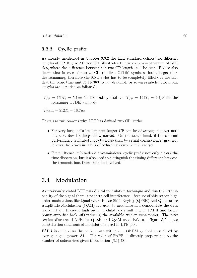
As already mentioned in Chapter 3.3.2 the LTE standard de�nes two di�erentlengths of CP. Figure 3.6 from [21] illustrates the time domain structure of LTEslot, where the di�erence between the two CP lengths can be seen. Figure alsoshows that in case of normal CP, the �rst OFDM symbols slot is larger thanthe remaining, therefore the 0.5 ms slot has to be completely �lled due the factthat the basic time unit Ts (15360) is not dividable by seven symbols. The pre�xlengths are de�nded as followed:

TCP = 160Ts = 5.1µs for the �rst symbol and TCP = 144Ts = 4.7µs for theremaining OFDM symbols

TCP−e = 512Ts = 16.7µs

There are two reasons why LTE has de�ned two CP lenths:

• For very large cells less e�cient longer CP can be advantageous over nor-mal one, due the large delay spread. On the other hand, if the channelperformance is limited more by noise than by signal corruption, it may notrecover the losses in terms of reduced received signal energy.

• For multicast or broadcast transmissions, cyclic pre�x not only covers thetime dispersion, but it also used to distinguish the timing di�erence betweenthe transmissions from the cells involved.

3.4 Modulation

As previously stated LTE uses digital modulation technique and due the orthog-onality of the signal there is no intra cell interference. Because of this reason highorder modulations like Quadrature Phase Shift Keying (QPSK) and QuadratureAmplitude Modulation (QAM) are used to modulate and demodulate the datatransmitted. However high order modulations result higher PAPR and largerpower ampli�er back o�s reducing the available transmission power. The nextsection discusses PAPR for QPSK and QAM modulations. Figure 3.7 showsconstellation diagrams of modulations used in LTE [30].

PAPR is de�ned as the peak power within one OFDM symbol normalized byaverage signal power [34]. The value of PAPR is directly proportional to thenumber of subcarriers given in Equation (3.1)[48].

3.4 Modulation 21

Figure 3.6: LTE time domain structure

PAPR(dB) ∝ log10N (3.1)

where

N is is the number of subcarriers

Large PAPR signal need high linear power ampli�ers to avoid modulation distor-tion, hence they have to operate with large back o� from their peak power whichresults low power e�ciency [38].

3.4.1 QPSK, 16-QAM and 64-QAM

In QPSK the modulation alphabet consists of four di�erent signaling choices,where a pair of two consecutive bits is converted from serial to parallel and thenmapped into its complex value constellation [39] as seen Figure 3.8. With QPSKup to two bits of information can be transmitted during each modulation symbolinterval. Assuming maximum amplitude A in both real and imaginary axis andunit average power, A can be calculated as follows [33]:

3.4 Modulation 22

Figure 3.7: LTE modulation constellations

Figure 3.8: QPSK constallation

4(A2 + A2)

4= 1

⇒ A =1√2

(3.2)

All the constellation points have the same power so PAPR can be calculated asshown:

PAPRQPSK =A2 + A2

1= 1 = 0dB (3.3)

This result can be seen as a constant envelope signal.

3.4 Modulation 23

Higher modulation like 16-QAM gives 16 di�erent alternatives (four bits persymbol), which allows up to four bits of information to be transmitted, therefore itis more bandwidth e�cient and permits higher data rates than QPSK. Figure 3.9shows the constellation diagram in two dimensional plane and again assumingunit average power the components can take amplitude values of 3A, A, −A and−3A, where A can be expressed as follows:

Figure 3.9: 16-QAM constallation

4(A2 + A2 + A2 + 9A2 + A2 + 9A2 + 9A2 + 9A2)

16= 1

⇒ A =1√10

(3.4)

And the maximum PAPR:

PAPR16−QAM =9A2 + 9A2

1= 1.8 = 2.55dB (3.5)

This means 16-QAM has a maximum PAPR of 2.55 dB with 25 % probability forthe four outer corner symbols. To obtain PAPR for four inner symbols is similarto equation (3.3), but for di�erent A value:

3.4 Modulation 24

PAPR16−QAM =A2 + A2

1= 0.2 = −7dB (3.6)

And PAPR for the remaining eight constallation points:

PAPR16−QAM =A2 + 9A2

1= 1 = 0dB (3.7)

In case of 64-QAM one have logically 64 di�erent choices (constellation points)shown in Figure 3.10. It maps six bit per symbol, hence it has three times largercapacity than QPSK. This modulation scheme is used in systems like 802.11 a/g.Again unit power is assumed and the amplitude values are 7A, 5A, 3A, A, −A,−3A, −5A and −7A and A is given using the same calculation method:

Figure 3.10: 64-QAM constallation

A =1√42

(3.8)

And the maximum PAPR:

3.4 Modulation 25

PAPR64−QAM =49A2 + 49A2

1=

98

42= 3.68dB (3.9)

Meaning the four outer symbols result a PAPR of 3.68 dB with 6.25 % (1/16)probability.

3.4.2 Pilot structure

One of the central problems in OFDM transmission is how to be able to trackand estimate multipath propagation environments. This is solved by puttingreference symbols also known as pilots in to the transmitted data. These symbolsare known to both transmitter and receiver; hence they are carrying no dataand are applied for proper channel estimation for each subcarrier. In LTE threetypes of reference signals are used [21]. Figure 3.11 illustrates the idea of insertedreference signals in two slots for cell speci�c reference symbols.

• Cell speci�c reference signals

• UE speci�c reference signals

• Broadcast reference signal

Figure 3.11: Structure of cell speci�c reference symbols

There are three main general uses for the reference symbols used in LTE [4]:

• Measuring the channel quality

• Channel estimation

• Initial acquisition and cell search

In the next chapter channel estimation will be discussed, since the referencesymbols are mainly used for channel estimation in the LTE simulation modelused for this Thesis.

3.4 Modulation 26

3.4.3 Channel estimation

Channel estimation is important part of LTE receiver design, since in order torecover the transmitted information correctly, one need to know, how the channelconditions are changed over time. The estimation of the channel e�ects is basedon an approximate underlying model of radio propagation channel [31]. Thereare di�erent channel estimation approaches used for pilot based estimation likeLeast Square (LS), Minimum Mean Square (MMSE) and Least Mean Square(LMS). This work describes the MMSE estimator, which is used in the MATLABsimulator model used in this thesis.

Generally OFDM transmission can be written in form of:

y = XFh+ n (3.10)

where

y is the received signal

X is diagonal matrix with data, reference symbols or zeros

F is FFT matrix

h is channel impulse response to be estimated

n is white Gaussian noise

Using the method described in [47] the Channel Impulse Response (CIR) can becalculated in equation (3.11), where they take advantage of auto covariance andthe cross covariance matrixes of the reference symbols.

h = RhYrR−1YrYr

Yr (3.11)

where

h is estimated CIR

Yr is received reference symbols without data or zeros

RhYr is cross covariance matrix of h and Yr

3.5 Link adaptation 27

RYrYr is auto covariance matrix of Yr

The covariance matrixes are calculated according to eqations (3.12) to (3.15) [36].For auto covariance matrix:

RYrYr = E[YrYHr ] (3.12)

= E[(XrFrh+ nr)(XrFrh+ nr)H ]

= E[(XrFrh+ nr)(XHr F

Hr h

H + nHr )]

= XrFrE[hhH ]XHr F

Hr + E[nrn

Hr ] +XrFr[hn

Hr ] + [nrh

H ]XHr F

Hr

= XrFrRhhXHr F

Hr + σ2

nInr (3.13)

and for the cross covariance matrix:

RhYr = E[hY Hr ] (3.14)

= E[hhHXHr F

Hr + nrh

HXHr F

Hr ]

= RhhXHr F

Hr

= XHr F

hr (3.15)

Putting it all into equation (3.11) CIR can be calculated as shown:

h = XHr F

Hr (XrFrRhhX

Hr F

Hr + σ2

nInr)( − 1)Yr (3.16)

3.5 Link adaptation

Basically there are two types of link adaptation, power and rate control. Powercontrol has been used in CDMA based mobile communication systems such asWCDMA. A variable transmit power is used to compensate the channel qualityvariations. The goal of power control is to maintain constant data rate at thereceiver. Basically transmit power is increased when the channel quality decreasesand vice versa if the conditions become more advantageous, so the transmit poweris inversely proportional to channel quality conditions as seen in Figure 3.12 (a).

3.5 Link adaptation 28

On the other hand in packet switched mobile communication services constantdata rate is not necessary needed, in many cases there is a need for rate ashigh as possible and this is the case where the modulation and coding rate isvaried depending on the channel conditions. This technique is called AdaptiveModulation and Coding (AMC). Short term data variations can be tolerated aslong as the average data rate remains constant, which is achieved by rate controlseen in Figure 3.12 (b)[21]. It can be shown that rate control is more e�cientthan power control therefore AMC is used in simulator written for this thesis anddescribed in detail below[28] and[26].

Figure 3.12: (a) Power control (b) rate control

3.5.1 Adaptive Modulation and Coding

In general the receiver chooses the best modulation and coding rate according tothe channel quality response from receiver via Channel Quality Indicator (CQI).In downlink eNodeB can select between QPSK, 16-QAM and 64-QAM and pos-sible coding rates listed in Table 5.4. There are basically two degrees of freedomfor AMC [46]:

• Modulaton Scheme: Low order modulation e.g. QPSK are more robustto poor channel conditions, but gives a lower transmission rate. On the

3.6 MIMO 29

other hand e.g. 16-QAM provides better transmission rate however is morevulnerable to channel conditions.

• Coding Rate: For given modulation di�erent coding rates can be chosenfrom Table 5.4. Lower coding rates are used for poorer channel conditionsand vice versa.

The reported CQI is calculated from pilot tones used in downlink transmission de-scribed in Chapter 3.4.2. The CQI, best Modulation and Coding Scheme (MCS),reported by UE is based on the Block Error Rate (BLER) probability not ex-ceeding 10 %. Simple method for UE to calculate best possible MCS can bebased on a BLER thresholds as seen in Figure 3.13. The UE selects the best CQIthat satis�es the condition BLER ≤ 10−1. Optimal switching points betweendmodulation order and coding rates depend on may di�erent factors like Qualityof Service (QoS) and cell throughput [46].

Figure 3.13: CQI Threshold example BLER ≤ 10−1

3.6 MIMO

Multiple input multiple output (MIMO) is one of the central technologies used inLTE to improve coverage, capacity, Quality of Service (QoS) and speci�ed datarates. It is a very large topic and this thesis describes only the basics of it. Formore detailed information please see the references used in this chapter e.g [18].

3.6 MIMO 30

MIMO operation includes techniques like spatial multiplexing, pre-coding andtransmit diversity which fundamentals will be discussed in this chapter.

3.6.1 Basics

The basic principles of MIMO as shown in Figure 3.14, where di�erent datastreams are transferred through pre-coder followed by signal mapping and OFDMsignal generation [30].

Figure 3.14: MIMO principle

The receiver antennas need to be able to separate the transmitted streams, there-fore reference symbols are used to separate them, where they are altered betweenantennas. For LTE standard 3GPP has speci�ed to cover up to four transmissionand reception antennas, hence as the number of antennas increases the neededSNR increases with the drawback of transmitter/receivers complexity as well asthe reference symbol overhead.

3.6.2 Spatial multiplexing

With MIMO technique an additional dimension to time and frequency is intro-duced named spatial dimension, which allows achieving the required peak datarates LTE has speci�ed. Data streams can be transmitted over di�erent parallelchannels using the same bandwidth and no additional power. The capacity islinearly related to the number of transmitter/receiver antenna pair.

The simultaneously transmitted bit streams cause interference at the receiver;hence di�erent interference cancelling techniques are used at the receiver, e.g.MMSE as described in Chapter 3.4.3. Figure 3.15 gives an example of 2x2 MIMOtransmission, where the received signal can be written as stated in eqation (3.17)[21].

3.6 MIMO 31

Figure 3.15: MIMO 2x2 example

Now the received signal r can be expressed in matrix form as:

r =

[r0

r1

]=

[h1,1 h1,2

h2,1 h2,2

] [s1

s2

]+

[n1

n2

]= Hs+ n (3.17)

where

H is 2x2 channel matrix

s is transmitted symbols

n is white Gaussian noise

Assuming no noise the transmitted symbols sk can be obtained at the receiverside as follows:

s =

[s0

s1

]=

1

h1,1h2,2 − h1, 2h2, 1

[h1,1 −h1,2

−h2,1 h2,2

] [r1

r2

](3.18)

3.6.3 Pre-coding

The basic idea in pre-coding is giving the transmitted signal from di�erent an-tennas di�erent weights in order to maximize the SNR at the receiver. The

3.6 MIMO 32

transmitter needs to know from the receiver about the channel conditions and forlarge MIMO systems this increases the overhead.

In open loop MIMO systems as the LTE simulator used in this work, one can usea set of pre-coding matrixes, which is known for both transmitter and receiver.This set of matrixes is also called MIMO codebook and noted as P , where L = 2r

is the size of it and r is the number of feedback bits needed for to index thecodebook [33]. After the MIMO system is speci�ed with a codebook, the receiverobserves the channel conditions and selects the best pre-coding matrix for thatcondition. The Pre-coding Matrix Index (PMI) is then reported back to thetransmitter as illustrated in Figure 3.16.

Figure 3.16: Closed loop MIMO system

An example of pre-coding matrixes for two antenna ports is described beneath,since LTE simualtor for this work uses the same codebook as described in [33].For the two antenna port pre-coding a grouping of 2x2 identity matrix and DFTmatrix is used, which for two antenna ports is described as follows:

W =1√2

[1 11 ejπ

]=

1√2

[1 11 −1

](3.19)

By introducing a shift parameter gGthe Fourier matrix can be written as follows:

Wg = ej2πmN

(n+ gG

) m,n = 0, 1, . . . (N − 1) (3.20)

Now a set of four 2x2 Fourier matrices can be de�ned for G = 4 and g ={0, 1, 2, 3}:

3.6 MIMO 33

W0 =1√2

[1 11 −1

](3.21)

W1 =1√2

[1 1

1+j√2

−1−j√2

](3.22)

W2 =1√2

[1 1j −j

](3.23)

W3 =1√2

[1 1−1+j√

2

1−j√2

](3.24)

In LTE, the codebook for two antenna ports includes seven di�erent code words,four rank 1 and three for rank 2, which are summarized in Table 3.3 [7]. Rank 1code words are just columns of rank 2 code words. The idea to limit the codebookalphabet only to {1, j} was to reduce the complexity of the UE in calculating theChannel Quality Indicator (CQI) by avoiding matrix calculations.

Codebook index Number of layersυ = 1 υ = 2

0 1√2

[11

]1√2

[1 00 1

]1 1√

2

[1−1

]12

[1 11 −1

]2 1√

2

[1j

]12

[1 1j −j

]3 1√

2

[1−j

]-

Table 3.3: LTE MIMO two antenna port codebook

3.6.4 Transmit diversity

Transmit diversity is basically sending multiple copies of the same signal in orderto exploit the gains from independent fading between the antennas. It is com-mon in downlink cellular systems; therefore it is cheap and easy to install moreantennas at the base station than to modify single UE, which may vary frommanufacturer to manufacturer. On the other hand in LTE because of the shorttransmission time of one sub-frame (1 ms), there is little time diversity available.

3.7 Multicodeword-MIMO HARQ 34

It can be exploited using Hybrid Automatic Repeat Request (HARQ) Protocol,which will be discussed in detail in Chapter 3.7. In the standardization phase ofLTE many transmit diversity schemes were discussed and evaluated, for detailedview of the di�erent techniques reader is adviced to see [33] Chapter 6.1.

To sum up the previously mentioned source, during the standardization and eval-uation phase in LTE there was a debate between two di�erent time diversitytechniques Cyclic Delay Diversity (CDD) [46] and block code based schemes suchas Alamounti space time coding [16]. CDD has a drawback with perfectly corre-lated antennas where there is no diversity available and block code based schemesdo not scale with the number of antennas, where the performance is penalized[33].

After long discussion the decision was made for block codes and for two antennaports Space Frequency Block Coding (SFBC) was speci�ed as a standard. Forfurther information see [40] and [32].

3.7 Multicodeword-MIMO HARQ

The basic idea behind ARQ is that the terminal may rapidly request a retransmis-sion if a transmission has been decoded with errors. In addition, HARQ providesa tool for rate adaption [21]. The di�erence between ARQ and HARQ protocol isthat HARQ is a combination of Forward Error Coding (FEC) and error detection.ARQ protocol only uses the error detection method. It is also to be noted, thatHARQ protocol is a function spread over both physical and MAC layer. MAClayer control the HARQ entity, where the combination and other bit operationsare done by the physical layer.

3.7.1 ARQ protocol categories

Di�erent types ARQ protocols can be divided into three categories:

• Stop-and-wait which is the simplest type of ARQ scheme. The transmitterwaits after sending a packet for an acknowledgment (ACK) or a negative ac-knowledgement (NACK) from receiver and then sends either a new packet,after receiving ACK or the same packet in case of NACK. Drawback of thismethod is the long waiting time at the transmitter waiting for ACK/NACK.

• Go-back-N has a de�ned window size where packets are sent without waitingfor an ACK. When NACK is received the transmitter starts to retransmitpackets from the missing packet, which in other words means, that possible


correctly decoded packets, after sending the missing packet for the �rsttime, are simply ignored and retransmitted again. This is also the biggestdrawback of Go-back-N, because of the duplicate transmissions of the samedata.

• Selective repeat protocols can handle this problem and keeps sending thepackets in de�ned window size. After receiving an NACK the protocolcontinues sending new packets and tries to resend only the corrupted one,therefore it has the best performance from the categories.

Since LTE has a modi�ed implementation of Stop-and-wait protocol it will bediscussed in detail. Figure 3.17 illustrates how the protocol works for one trans-mission process. As seen in the illustration the problem is the long waiting time,where the transmitter is idle waiting for ACK/NACK report. On the other handthe receiver only has to bu�er one packet at the time that is currently beingdecoded.

Figure 3.17: ARQ stop-and-wait protocol

LTE uses multiple parallel Stop-and-wait processes. In standard eight parallelprocesses are speci�ed see equation (3.25). After receiving a transport blocktransmitter tries to decode the block and informs transmitter with an informa-tion bit if block number was successfully decoded respectively not. Additionally


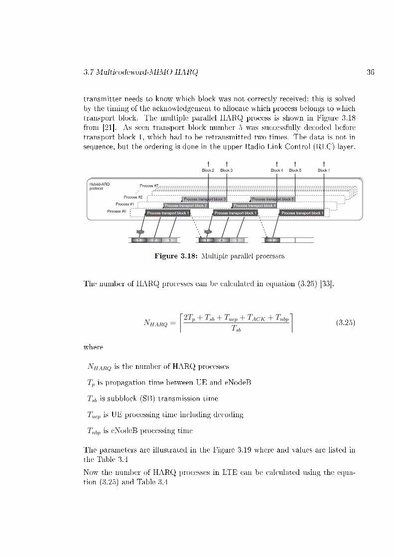
transmitter needs to know which block was not correctly received; this is solvedby the timing of the acknowledgement to allocate which process belongs to whichtransport block. The multiple parallel HARQ process is shown in Figure 3.18from [21]. As seen transport block number 5 was successfully decoded beforetransport block 1, which had to be retransmitted two times. The data is not insequence, but the ordering is done in the upper Radio Link Control (RLC) layer.

Figure 3.18: Multiple parallel processes

The number of HARQ processes can be calculated in equation (3.25) [33].

NHARQ =

⌈2Tp + Tsb + Tuep + TACK + Tnbp

Tsb

⌉(3.25)

where

NHARQ is the number of HARQ processes

Tp is propagation time between UE and eNodeB

Tsb is subblock (SB) transmission time

Tuep is UE processing time including decoding

Tnbp is eNodeB processing time

The parameters are illustrated in the Figure 3.19 where and values are listed inthe Table 3.4

Now the number of HARQ processes in LTE can be calculated using the equa-tion (3.25) and Table 3.4


Figure 3.19: Stop-and-wait HARQ round trip time (RTT)

Parameter Symbol ValuePropagation time Tp Neglible

Sunbblock transmission time Tsb 1 msUE processing time Tuep 3 ms

ACK transmission time TACK 1 mseNodeB processing time Tnbp 3 ms

Table 3.4: LTE HARQ RTT paremeters

NHARQ =

⌈0 + 1 + 3 + 1 + 3

1

⌉= 8 (3.26)

In LTE the erroneously decoded blocks are kept at the receiver's bu�er, hence thepartly available data can be used with the retransmitted packet. HARQ schemesupport so called Chase combining and incremental redundancy methods to dealwith the retransmission at the receiver's side. These methods will be discussedin Chapter 3.7.2.

HARQ protocols can be characterized in synchronous vs. asynchronous and �ex-ible vs. non �exible depending on the resource usage and link adaptation [21].

Asynchronous retransmission can occur at any time, whereas synchronous re-transmissions happen at certain �xed time after previous transmission. There-fore asynchronous protocol has more �exibility, but the usage of synchronousretransmission does not require any explicit HARQ process number signaling asthe information can be extracted from the sub frame number.

The adaptive protocol takes the frequency resources into account, where moresuitable transmission format can be selected. Non adaptive protocol on the other


hand uses the same frequency resources as the same transmission format as theinitial transmission.

3.7.2 Chase Combining and Incremental Redundancy

The simplest form of HARQ scheme was proposed by Chase in 1985 [19]. It canbe seen as additional repetition coding, since no new redundancy is transmitted.At each retransmission exact copy of the information bits are transmitted andcombined at the receiver using maximum ratio combining. Chase combiningdoes not give additional coding gain, it only increases the received Eb

N0for each

retransmission, where Eb is energy over bit and N0 spectral noise density. Forfurther details about Eb

N0see [41]. Figure 3.20 from [21] shows an example of using

Chase combining.

Figure 3.20: Example of Chase combining

In case of Incremental redundancy (IR) the retransmission bit do not have to bethe same then di�erent sets of coded bits are transmitted each having the sameamount of information bits [44]. In case of retransmission di�erent set of bits fromprevious transmission are sent, combined and sent to decoder. Retransmissionbits do not necessarily need to have the same modulation scheme as the previous.With IR low rate coding is often used and the di�erent retransmission set of bitsare generated by puncturing the encoder output bits. Figure 3.21 from [21] showsan example with a 1/4 code rate, where at the �rst retransmission every third


coded bit is sent at rate 3/4. In case of decoding error a new set of bits is createdgiving a rate of 3/8. After second retransmission the rate will be 1/4 and for anyfurther retransmission the information bits will be repeated. IR not only gives again in Eb

N0, but it also achieves a coding gain for each retransmission.

Figure 3.21: Example of Incremental redudancy

Comparison of Chase and IR shows that IR achieves a larger gain at higherinitial coding rates while for lower rates both techniques are more or less equal[20]. Moreover the performance gain of IR compared to Chase combining canalso depend on the relative power di�erence between the transmission attempts[24].

3.7.3 Multicodeword-MIMO HARQ alternatives

In LTE three di�erent retransmission schemes were discussed [3], which perfor-mance is the main scope of this thesis and discussed in detail in the next chapters:

• Independent processes

• Blanking

• Non-blanking


3.7.3.1 Independent

Independent HARQ process means in case of two antenna ports that both arehaving their own HARQ process and are working totally independent from eachother. Table 3.5 shows an example of two independent processes for two antennasA and B. Each antenna gets their own ACK/NACK for the transmitted codewordand retransmit it in case of NACK.

Antenna A A1 NACK A1 ACK A2 ACK A3 NACK A3 ACK A4

Antenna B B1 ACK B2 ACK B3 NACK B3 NACK B3 ACK B4

Table 3.5: Independent HARQ transmission example

Codewords Ak and Bn are transmitted independently and in every time slot bothantennas are sending a codeword to the receiver. This transmission scheme hasthe best performance compared to the next two, but there is hardly any literatureabout the performance di�erence compared to the other schemes except in [3],where blanking method is shown as being the worst in terms of throughput. Thecomparison of these three HARQ cases is the main topic of this thesis.

3.7.3.2 Blanking

In this transmission scheme there is only one HARQ process but two ACK/NACKfor two antennas. Table 3.6 shows an example transmission.

Antenna A A1 NACK A1 ACK A2 ACK ACK A3 ACK A4

Antenna B B1 ACK ACK B2 NACK B2 ACK B3 ACK B4

Table 3.6: Blanking HARQ transmission example

As seen in the table, if one packet is correctly decoded and the other one not, onlythe erroneously decoded codeword is resent (A1) and the other antennas codewordis left blank (no B2). This makes it more probable for the sent codeword to arrivecorrectly at the transmitter, since there is no other message to interfere with thedata.

3.7.3.3 Non-blanking

In last non-blanking transmission scheme there is only one ACK/NACK for twocodewords. Again a transmission example is shown in Table 3.7.


Antenna A A1 n A1 a A2 a A2 a A2 a A3

NACK ACK NACK NACK ACKAntenna B B1 a B1 a B2 n B2 n B2 a B3

Table 3.7: Non-blanking HARQ transmission example

The n and a indicates that codeword from that antenna was decoded correctly,but since there is only one ACK/NACK and only one codeword has been decodedcorrectly, the transmitter gets a NACK and resends both messages again and doesnot leave empty (blank) spaces in order the get the erroneously decoded codewordhigher probability to get through. This is seen in the example tables where inblanking transmission scheme B2 does not get interfered by antenna A and needsonly be retransmitted one, where in non-blanking scheme B2 has to be sent threetimes.

Chapter 4

LTE Downlink

This chapter discusses the functions of the di�erent layers in LTE downlink, wheredata is sent from base station to the mobile terminal. Figure 4.1 illustrates theLTE layer structure [21]. The simulator used in this work has only the two lowestlayers implemented; nevertheless this chapter will discuss also the third layernamed Radio Link Control (RLC) brie�y to give the reader a better overview ofthe functionality.

Then more on detailed view of layer 2 the Medium Access Control (MAC) willfollow including multiplexing and mapping di�erent channels to communicatewith the lowest layer the Physical Layer (PHY). MAC layers other functionaliteslike scheduling and discontinuous reception are also reviewed as well as the mainfocus of this thesis the HARQ entity, which is split over MAC and PHY layers.

Moving further to lowest layer the Physical Layer its important functions likechannel coding with Cyclic Redundancy Check (CRC) and turbo coding are dis-cussed. Nevertheless OFDM modulation is revised and �nally HARQ functionsat the PHY layer level are described.

4.1 RLC Layer

RLC is located between Packet Data Convergence Protocol (PDCP) and MAClayer and it communicates with the upper one using Service Access Point (SAP)and with the lower one via logical channels. RLC is responsible for segmentationof RLC Protocol Data Units (PDU) from PDCP into Service Data Units (SDU)suitable size for MAC layer as shown in Figure 4.2 from [21].

RLC is also responsible for retransmission of wrongly received PDUs and remov-

42

4.1 RLC Layer 43

Figure 4.1: LTE downlink architecture

Figure 4.2: RLC PDU to SDU segmentation

ing the duplicate ones. Hence it manages the in sequence delivery of SDUs forthe upper layers. The functions of RLC are performed by RLC entities, whichcan be con�gured in three di�erent modes:

• Transparent Mode

• Unacknowledged Mode

• Acknowledged Mode

4.2 MAC Layer 44

For further details to RLC Layer functionality reader is adviced to see [46].

4.2 MAC Layer

MAC layer is the second lowest layer in the LTE architecture and communicateswith RLC through logical channels and with physical layer through transportchannels; therefore it performs multiplexing and demultiplexing between thosechannels. Figure 4.3 from [46] gives an overview about the MAC layer functions,hence it can be considered as a controller with multiplexing and HARQ entity.

Figure 4.3: Overview of LTE MAC layer

4.2.1 Multiplexing and mapping

As already stated above MAC layer communicates with logical and transportchannels which need to be mapped correctly when transferring to other layers.Following logical channels for downlink are speci�ed for LTE [9]:

• Broadcast Control Channel (BCCH) which is used to broadcast system in-formation.

4.2 MAC Layer 45

• Paging Control Channel (PCCH) which noti�es UEs of an incoming call orchange of system information.

• Common Control Channel (CCCH) which delivers control information whenthere is no con�rmed association between UE and the eNobeB.

• Multicast Control Channel (MCCH) which transmits control informationrelated to reception of broadcasting information.

• Dedicated Tra�c Channel (DTCH) which transmits dedicated user data.

• Multicast Tra�c Channel (MTCH) which transmits user data of broadcastservices.

On the other hand following transport channels in downlink direction are de�nedin [9]:

• Broadcast Channel (BCH) which is used to transport parts of system infor-mation for DL-SCH.

• Downlink Shared Channel (DL-SCH) which transport downlink user dataor control messages.

• Paging Channel (PCH) which transports paging information to UEs.

• Multicast Channel (MCH) which transports user data or control messagesrelated to multicasting or broadcasting.

Figure 4.4 illustrates the 3GPP speci�cation of channel mapping und multiplexingin downlink direction. It can be seen that DL-SCH carries information from allthe logical channels with exception of PCCH.

4.2.2 Scheduling

One of the basic principles of LTE is that time and frequency resources are dy-namically shared between the users. Scheduler is in charge of assigning and con-trolling the resources. The signals used for scheduling are standardized by 3GPP,but the details are left for the eNodeB implementation. Basically a terminal lis-tens to the scheduling commands received from a unique serving cell which every1 ms TTI makes a scheduling decision and sends it to the UE. These commandsinclude transport block size, modulation scheme, antenna mapping and logicalchannel multiplexing. Figure 4.5 from [21] shows the transport format selection

4.2 MAC Layer 46

Figure 4.4: Downlink logical to transport channel mapping

in downlink transmission. The basic time frequency unit in scheduler is called aresource block which spans of 180 kHz and in each 1 ms those blocks are assignedto DL-SCH.

Figure 4.5: Downlink scheduling

The main idea of the scheduler, since it can exploit channel variations in timeand frequency domain, is to schedule a transmission to a terminal with the best

4.3 PHY Layer 47

channel conditions. Especially for low speed UEs where time domain channelvariations not likely to change fast, the frequency domain channel variations canvary signi�cantly, which gives LTE scheduler an advantage over earlier generationtechnologies like HSPA.

4.2.3 Discontinuous Reception (DRX)

To save UE battery DRX has two states con�gure connected and idle so that UEdoes not always have to monitor the downlink channels. The parameterizationof DRX is a tradeo� between UEs battery life and latency e.g. for sur�ng theweb and viewing a single webpage it is not bene�cial to continuously receiveinformation from the downlink channels, since the data showing the page hasalready been loaded on the device. On the other hand shorted idle period givesa faster response if new data has to be captured.

4.2.4 HARQ

HARQ provides robustness against transmission errors and as seen in Figure 4.3it is a part of MAC layer functions but also a part of physical layer. There isonly one HARQ entity at UE which handles number of parallel HARQ processes,where each process is associated with a HARQ identi�er. HARQ is not applicablefor all of the tra�c; hence in downlink only for DL-SCH. HARQ function onMAC layer speci�es which soft combining (Chase Combining (CC) or IncrementalRedundancy (IR)) and which type of HARQ (independent, blanking or non-blanking) should be used. HARQ functionality on the physical layer is describedin Chapter 4.3.3.

4.3 PHY Layer

The LTE physical layer is the lowest layer before sending the data from basestation, also called enhanced NodeB (eNodeB) to UE. In downlink direction it isresponsible for Cyclic Redundancy Check (CRC), coding, rate matching, modula-tion and mapping e.g. transport channels into physical channels as stated before.Figure 4.6 from [14] shows an overview of physical layer downlink transmissionand its functions, which will be described in detail in the upcoming chapters.

4.3 PHY Layer 48

Figure 4.6: Physical layer function in downlink transmission

4.3.1 Channel coding

Channel coding is used to increase the reliability of the channel by adding redun-dancy to the information transmitted with the drawback of reducing the infor-mation rate.

4.3.1.1 CRC

In �rst step of physical layer downlink processing a 24 bit CRC is calculated foreach data block for error detection at the receiver. If CRC detection fails at thereceiver, e.g. HARQ will inform the transmitter about failed transmission andrequests a retransmission according to which type of HARQ is used. If the inputbits of a length A are listed as a0, a1, . . . , aA−1 and the parity bits of length Lare denoted by p0, p1, . . . , pL−1. The parity bits are generated by using e.g. thefollowing cyclic generator polynomial [10].

gCRC24B(D) =[D24 +D23 +D6 +D5 +D + 1

](4.1)

The encoding is performed in systematic form, where the polynomial

4.3 PHY Layer 49

a0DA+23 + a1D

A+22 + . . .+ aA−1D24 + p0D

23 + p1D22 + . . .+ p22D

1 + p23 (4.2)

is divided by corresponding 24 bit CRC polynomial and yields a remainder equalto 0:

a0DA+14 + a1D

A+14 + . . .+ aA−1D16 + p0D

15 + p1D14 + . . .+ p14D

1 + p15 (4.3)

4.3.1.2 Turbo coding

Berrou, Glavieux and Thitimajasimha presented turbo codes and concept of itera-tive decoding to achieve near Shannon limit performance in 1996 [17]. It performsbetter than any other encoder at very low SNR. Turbo encoder consist two eightstate convolutional encoders linked by an interleaver. LTE standard speci�es aParallel Concatenated Convolutional Code (PCCC) encoder with a coding rateof 1/3 and transfer function [10]:

G(D) =

[1,g1(D)

g0(D)

](4.4)

where

g0(D) = 1 +D2 +D3 = [1011]

g1(D) = 1 +D +D3 = [1101]

Figure 4.7 illustrates the structure of 1/3 turbo encoder used in LTE. The outputof the turbo encoder is given in equation (4.5).

d(0)k = xk, d

(1)k = zk, d

(2)k = z′k k = 0, 1, . . . , K − 1 (4.5)

where

K is the number of input bits

4.3 PHY Layer 50

xk are called systematic bits

zk are called �rst partity bits

z′k are called second parity bits

The input bits respectively the output bits for the encoders interleaver are de-noted c0, c1, . . . , cK−1 respectively c0, c1, . . . , cK−1 and the relationship is listed inequation (4.6) and (4.7).

c′i = cΠ(i) i = 0, 1, . . . , K − 1 (4.6)

Π(i) =(f1i+ f2i

2)modK (4.7)

The parameters f1 and f2 depend on the block size K and stated in the Table5.1.3-3 in [10]. LTE turbo encoder has the maximum block size of 6144 bits, ifthis number is exceeded the code block is split into smaller ones and again newCRC is generated before going through the turbo encoder. For simplicity reasonsthe simulator was implemented with the maximum code block size of 6144 bits.

In LTE downlink direction adaptive modulation and coding schemes are used,which means di�erent number of coded bits can change depending on the retrans-mission and channel conditions. With turbo codes, its performance is sensitiveto the systematic bits; hence they should be transmitted in the �rst transmis-sion attempt. To meet this requirements LTE uses so called circular bu�er ratematching which is illustrated in Figure 4.8 from [46].

The from turbo encoder generated systematic bits (systematic) and two streamsof parity bits (parity0 and parity1) are interleaved separately by so called subblock interleavers. The redundancy version (RV) starting from 0 sends as manysystematic bits as possible. For retransmission, meaning further redundancy ver-sions, the parity bits are alternately inserted into the message to increase theredundancy.

4.3.2 Modulation

As already stated in Chapter 3.4 depending on the channel conditions LTE canuses di�erent modulation order starting from QPSK up to 64-QAM. This is doneby the modulation mapper as written in LTE standard in Chapter 7 in [11].Figure 4.9 from [22] shows a discrete OFDM system model.

4.3 PHY Layer 51

Figure 4.7: LTE turbo encoder structure

The data bits are grouped into block of Nc data symbols which can be written as avectorX. When performing IDFT or IFFT a cyclic pre�x of length Ncp is insertedinto X. The resulting signal can be mathematically described in equation (4.8).

s(n) =

1Nc

Nc−1∑k=0

Xkej2πk(n−Ncp)

Nc . n ∈ [0, Nc +Ncp − 1]

0 otherwise

(4.8)

4.3.3 HARQ

In LTE downlink asynchronous adaptive HARQ with soft combining is used seeChapter 3.7, therefore the erroneous packets are bu�ered at the receiver to com-bine it with the retransmission bits and to decode the message correctly. HARQused in simulator for this thesis uses Chase combining method; where at eachretransmission same message is sent and combined with the previous, not suc-cessfully decoded, message to increase the probability of correct transmission. Anexample of Chase combining was given in Figure 3.20.

4.3 PHY Layer 52

Figure 4.8: LTE rate matching for turbo codes

Figure 4.9: Discrete OFDM system model

Each HARQ process has three control information �elds carried with the trans-mission [5]:

• New data indicator (NDI): Is toggled when new data is delivered - 1 bit

• RV : Which redundancy version is used - 2 bits

• Modulation and coding scheme (MCS): Which modulation and coding schemeis used - 3 bits

Chapter 5

Simulator

In next section of this chapter the simulation model from basic overview to moredetailed functionality of the main elements in communication systems, transmit-ter, channel and receiver is introduced.

Furthermore di�erent channel models used, e.g. Winner II, in the simulations areintroduced and shown how they are implemented.

At the end the for thesis written simulator is veri�ed to provide correct simulationresults including correct modulation, HARQ functionality, transmit diversity, linkadaptation and MIMO transmission.

5.1 System model

Figure 5.1 illustrates the model used in the simulator build for this thesis. Asseen there is one transmitter (eNodeB) and one receiver (UE) and the UE isaccepting data from eNodeB (downlink). In between there is a channel which canbe selected from di�erent International Telecommunication Union (ITU) channelmodels described in section 5.1.2.

Figure 5.2 shows the simulation �ow, where at �rst simulation parameters areinitialized including SNR, channel model, number of drops, number of framesetc.. First loop is made over initialized SNR values e.g. from 10 to 50 dB with 10dB steps. Next loop is made over drops, meaning user is dropped in random placeinside a cell and moved according to the set speed at the initialization processe.g. 3 km/h. The drop loop is followed by frame loop, where the number of sentframes is speci�ed at the beginning of the simulation e.g. 100 frames. Then thetypical sending and receiving process occurs, by sending data from transmitter

53

5.1 System model 54

Figure 5.1: System model overview

over a certain channel conditions e.g. PedestrianA and received at UE. Beforeending the frame loop statistics over the sent packets is collected for further use.After ending frame and drop loops the collected statistic data is summed up andvalues like Bit Error Rate (BER) and throughput are calculated, before startingthe next SNR value loop. The simulation ends when SNR loop has run throughall its values and the simulation results are saved for further use.

Figure 5.2: LTE Downlink simulation �ow

5.1 System model 55

5.1.1 Transmitter

Figure 5.3 shows the implemented 2x2 MIMO transmitter, where two randombinary streams are mapped into di�erent constellation diagrams and modulatedwith di�erent subcarrier frequencies. Then as described for later channel estima-tion known pilot tones are inserted into the OFDM resource grid. Next signalspectrum length is increased by adding zeros and run through an IFFT blockfollowed by cyclic pre�x insertion as described in Chapter 3.3.3. Finally thetransport blocks are mapped into the di�erent antennas and sent to the receiver.

Figure 5.3: LTE Downlink 2x2 MIMO transmitter

5.1.2 Channel

The transmitted signal in real world results multipath propagation caused byfollowing basic mechanisms:

• Line of sight propagation

• Specular re�ections

• Di�raction caused by bending electromagnetic waves

• Di�usion or scattering

• Partial absorbtion e.g. transmission through objects

5.1 System model 56

In the real world the number of paths is unknown, but for simulation purposesthe number of paths is �xed enabling channel modeling. Good channel modelsare essential for analysis, design and development of telecommunication systems.The more realistic the model is the better the correlation between simulation andreal world. There are many channel models to choose from. The next sectiondiscusses the ones used in the simulator.

The channel models are described as taps, where each taps corresponds to acertain delay and power. For the simulator the channel power values need to benormalized which is done in equation (5.1).

Ak =

√√√√√√Pi

N∑k=1

Pk

(5.1)

where

Ak is the channel tap normalized amplitude

Pi is the channel tap linear scale power

N is number of taps

5.1.2.1 Winner II model

For the �nal simulations, a special channel model with �at and short frequencyresponse is used in order to see the di�erences between the simulation cases.The parameters for the Winner II channel model are taken from [42] and listedin Table 5.1. Winner II channel model is a suitable model for mobile indoorcommunication which adds some more actuality into this thesis.

5.1.2.2 Typical Urban model

Table 5.2 shows a six tap GSM typical urban channel, which in this thesis wasused for MIMO 2x2 transmission veri�cation [13].

5.1 System model 57

Delay [ns] Power [dB]0 -15.25 -19.75 -15.15 -18.815 -16.315 -17.715 -17.120 -21.2l25 -13.040 -14.680 -23.085 -25.1110 -25.4115 -24.8150 -33.4175 -29.6

Table 5.1: Winner II channel model parameters

Delay [µs] Power [dB]0 -30.2 00.5 -21.6 -62.3 -85.0 -10

Table 5.2: GSM 6 ray typical urban channel model parameters

5.1.3 Receiver

The receiver used in simulator has basically the same structure but opposite as inFigure 5.3 used transmitter. Instead of mapping demapping is used, cyclic pre�xand padded zeros are removed and the received data is put through FFT blockfor demodulation.

It is to be noted, that at the receiver an MMSE channel estimator, as describedin Chapter 3.4.3, is used to give feedback for the transmitter about the channelcondition via Channel Quality Indicator (CQI) if higher modulation order can be

5.1 System model 58

used to achieve better throughput.

5.1.4 Simulator veri�cation

To ensure the informative value of the simulations, the used modules need tobe veri�ed by testing them separately before putting them together. In thissection �rstly the modulation and demodulation is tested to be working correctlyby comparing the simulated Bit Error Rates (BER) with the BERs found in theliterature before moving to HARQ veri�cation, transmit diversity, link adaptationand MIMO transmission.

For modulation veri�cation simple transmission scenarios are simulated and com-pared with known results from the theory e.g. one tap Rayleigh and AdditiveWhite Gaussian Noise (AWGN) channel are used to control the (BER) for givenSNR values. These channel models are well known in the theory and the resultscan be easy compared to the theoretical values. Modulations used for BER veri-�cation are QPSK, 16-QAM and 64-QAM and the equations are taken from [27].Table 5.3 shows parameter settings used for BER simulations.

First we de�ne:

γ =EbN0

(5.2)

Q(x) =1

2erfc

(x√2

)=

1√π

∫ ∞x√2

e−t2

dt (5.3)

P (γ, L) =1

2L

(1−

√γ

1 + γ

)L L−1∑k=0

(L− 1 + k

k

)1

2k

(1 +

√γ

1 + γ

)k(5.4)

where

Eb is energy over bit

N0 is spectral noise density

erfc(x) is complementary error function

L is number of branches

5.1 System model 59

Parameter ValueBandwidth 5 MHzModulation QPSK, 16-QAM or 64-QAMChannel AWGN or RayleighNumber of drops 50Number of frames 100FFT size 512Number of subcarriers 300Cyclic pre�x NormalHARQ NoLink adaptation NoPre-coding NoNumber of Tx antennas 1Number of Rx antennas 1

Table 5.3: Basic simulation settings for BER simulation

5.1.4.1 BER QPSK

The bit error rate function for QPSK modulation for AWGN channel is shown inequation (5.5):

Pb = Q(√

2γ)

(5.5)

and for Rayleigh channel:

Pb = P (γ, L) (5.6)

The theoretical values and simulation results are compared in Figure 5.4.

5.1.4.2 BER 16-QAM

For Gray encoded 16-QAM modulation the bit error rate function for AWGNchannel is:

5.1 System model 60

Figure 5.4: BER for QPSK modulation

Pb =3

4Q

(√4

5γ

)+

1

2Q

(3

√4

5γ

)− 1

4Q

(5

√4

5γ

)(5.7)


Pb =3

4P

(2

5γ, L

)+

1

2P

(18

5γ, L

)− 1

4P (10γ, L) (5.8)


5.1.4.3 BER 64-QAM

Again for Gray encoded 64-QAM modulated signal BER function for AWGNchannel is described as:

Pb =7

12Q

(√2

7γ

)+

6

12Q

(√18

7γ

)− 1

12Q

(√50

7γ

)+

1

12Q

(√162

7γ

)− 1

12Q

(√338

7γ

)(5.9)

5.1 System model 61

Figure 5.5: BER for 16-QAM modulation


Pb =7

12P

(1

7γ, L

)+

6

12P

(9

7γ, L

)− 1

12P

(25

7γ, L

)+

1

12P

(81

7γ, L

)− 1

12P

(169

7γ, L

)(5.10)


5.1 System model 62

Figure 5.6: BER for 64-QAM modulation

The simulation results as shown in �gures show good results where the simulatedBER results are very close to the theoretical values. These tests con�rm themodulation and demodulation working properly and the results received fromthe simulator are reliable. The small variation from theoretical results seen onRayleigh channel BER curves can be explained by channels random number gen-erator. To plan those it would need much more channel sent frames, but sincethe curves are very close to the theoretical values it is not considered as a neededprocedure.

5.1.4.4 HARQ functionality

The HARQ functionality can be veri�ed with various throughput simulations de-pending on SNR, where di�erent throughput curves for di�erent coding rates aresimulated without HARQ functionality and then compared with the HARQ sim-ulation throughput. The HARQ throughput should adapt to the best throughputcurve for the given SNR.

To test the HARQ functionality QPSK modulation with di�erent coding rates inAWGN channel was chosen and all other parameters used in simulation are thesame as presented in Table 5.3. Table 5.4 from [12] shows according to whichCQI index which modulation and coding rate is used in LTE standard.

Firstly, CQI indexes from one to six were simulated in an AWGN channel withoutHARQ retransmissions and throughput calculated and plotted as illustrated in

5.1 System model 63

CQI Index Modulation code rate x 10240 out of range1 QPSK 782 QPSK 1203 QPSK 1934 QPSK 3085 QPSK 4496 QPSK 6027 16-QAM 3788 16-QAM 4909 16-QAM 61610 64-QAM 46611 64-QAM 56712 64-QAM 66613 64-QAM 77214 64-QAM 87315 64-QAM 948

Table 5.4: CQI Index table

Figure 5.7.

Second the shannon capacity is calculated using the following equation:

C = FB log2 (1 + SNR) (5.11)

where

C is system capacity (Shannon capacity)

B is bandwidth occupied by the data subcarriers

SNR is Sigal-to-Noise-Ratio

F is a correcting factor to cover some system losses

The bandwidh B is calculated according to [35]:

B =NscNsNrb

Tsub(5.12)

5.1 System model 64

where

Nsc is number of subcarriers in one resource block

Ns is number of OFDM symbols in one subframe

Nrb is number of resource blocks in selected system bandwidth

Tsub is the duration of one subframe

The correction factor F including CP and pilot sequence insertion losses [35]:

F =Tframe − TCP

Tframe

NscNs/2− 4

NscNs/2(5.13)

where

Tframe is frame duration

TCP is total CP time of all OFDM symbols in one frame

For this HARQ simulation number of subcarriers was set to Nsc = 11, numberof OFDM symbols Ns = 14, number of resource blocks Nrb = 25, length ofa subframe Tsub = 1 ms, length of a frame Tframe = 10 · Tsub = 10 ms andTCP = 20 · 7 · 4.7 · 10−6s = 658 µs. The shannon capacity was plotted togetherwith CQI indexes in Figure 5.7.

Next QPSK modulation with the highest coding rate was selected (CQI = 6)and HARQ functionality with Chase combining (CC) with maximum of threeHARQ retransmissions was switched on and the simulation was run again andthroughput plotted with the previous results. The number of drops and framesfrom Table 5.3 was changed to �ve respectively 1000 to minimize the numberof lost statistic frames e.g. if 50th frame transmission is not successfull and theframe should be retransmitted with HARQ, it is lost because of reached numberof maximum frames in that drop .The results are shown in Figure 5.8.

Figure 5.9 shows an example of HARQ where it is easier to calculate which coderate curves it will adapt to. The simulation is run under same conditions asthe previous, AWGN channel with �ve drops and 1000 frames to be calculated;nevertheless the coding rate is changed. The coding rate is 2/3, which doesnot correspond to a CQI in the LTE standard as seen in Table 5.4, but it wasimplemented in the simulator to better see the di�erent coding rates that HARQ

5.1 System model 65

Figure 5.7: QPSK throughput for di�erent coding rates

Figure 5.8: QPSK throughput with HARQ CC CQI = 6

First Tx 1. reTx 2. reTx 3. reTxCoding rate 2

313

29

16

Table 5.5: QPSK coding rates

5.1 System model 66

Figure 5.9: QPSK coding rate 2/3 throughput with HARQ IR

utilizes before reaching its maximum throughput. Table 5.5 shows the codingrates which are realized with QPSK rate 2/3 after each retransmission.

It is shown in the Figure 5.8 the bene�t on HARQ, without HARQ for CQI = 6 thethroughput is larger than zero around SNR = 2 dB, but with retransmissions datacan already be correctly encoded at SNR = -5.5 dB. As stated at the beginning ofthe section, the throughput curve adapts to the best �tting CQI curve as far thecoding rates are matching. One can see around SNR = -3 and -1 dB, the curveis not achieving its maximum throughput value. This e�ect is caused by Chasecombining used for retransmission, where not only data, but redundancy bits areresent. This phenomenon is called SNR loss. As a result HARQ implementationcan be considered as working properly.

5.1.4.5 Transmit diversity

For transmit diversity testing two transmission antennas with QPSK modulation(CQI = 5) were added into simulation, where Rayleigh one tap channel was usedand BER curve calculated. Transmit diversity should result to so called SNRgain, where the BER curve is moved to the left, meaning better BER rate isachieved at the receiver side. Figure 5.10 shows the simulation result comparedwith single antenna QPSK modulation over Rayleigh one tap channel.

One can see from Figure 5.10 the SNR gain provided by transmit diversity, theBER curve is shifted to the left giving better BER for given SNR. Therefore

5.1 System model 67

Figure 5.10: QPSK Trasmit diversity vs QPSK single antenna Rayleigh channel

transmit diversity can be assumed as working properly.

5.1.4.6 Link adaptation

Link adaptation was tested at system bandwidth set to 5 MHz without channelestimation (no pilot tones used). As a reference Figure 5.7 was used, wherethroughput curves with di�erent coding rates using QPSK modulation (CQI =1 to CQI = 6) were plotted. Using link adaptation should pick the best CQImatching the current SNR value and as an outcome one should get a curve �ttingthe best coding rate and throughput for given SNR e.g for SNR = 1 dB linkadaptation must pick CQI = 5. Figure 5.11 shows the simulation results.

Figure 5.11 shows how link adaptation chooses the correct coding rate for thegiven SNR and adapts to the best possible throughput curve. Therefore the resultcon�rms link adaptation working correctly and can be assumed as implementedin proper way.

5.1.4.7 MIMO transmission

For MIMO transmission veri�cation a reference article [1] Table 2 was used tocompare their throughput results with the simulator. The simulation was madefor three di�erent modulation QPSK, 16-QAM and 64-QAM with di�erent codingrates and the maximum throughput was compared with the results from the

5.1 System model 68

Figure 5.11: Link adaptation test with no channel estimation

reference. The calculation were made in AWGN channel with system bandwidhof 20 MHz and number of resource block was set to Nrb = 100. The results arelisted in Table 5.6 as throughput in Mbps and spectral e�ciency in bit/Hz/s.

Simulator Reference[Mbps] [bit/Hz/s] [Mbps] [bit/Hz/s]

QPSK 1/2 30.4 2.00 31.1 1.99QPSK 3/4 45.6 3.00 46.9 3.01QPSK 4/5 48.7 3.20 50.1 3.2116-QAM 1/2 60.8 4.00 62.6 4.0116-QAM 2/3 81.1 5.34 83.4 5.3516-QAM 3/4 91.2 6.00 93.8 6.0164-QAM 2/3 121.6 8.00 125.1 8.0264-QAM 3/4 136.8 9.00 140.8 9.0364-QAM 4/5 145.9 9.60 150.2 9.63

Table 5.6: MIMO 2x2 Throughput ver�cation

The simulation results are close to the reference. The di�erence between thethroughputs can be explained by the subcarrier usage in shared channel andbandwidth allocation in both systems. Equation (5.14) shows how the throughputcan be calculated from modulation order, coding rate and subcarrier usage inshared channel.

5.1 System model 69

Tr = NbitsRNsub (5.14)

where

Tr is throughput

Nbits is number of bits per symbol

R is code rate

Nsub is number of subcarriers per second

As an example for subcarrier usage, calculation 64-QAM with coding rate 4/5is taken from Table 5.6. For 145.9 Mbps Nsub ≈ 30400 subcarriers/ms for bothstreams, divided by two because of MIMO transmission one gets 15200 subcarri-ers/ms for one stream for 20 MHz system bandwidth. Same calculation for thevalues taken from [1] the number of subcarriers for one stream is approximately15600 subcarriers/ms.

The MIMO system theoretical capacity is calculated using equation (5.11), butthe logarithm term is replaced by the term shown in equation (5.15) which is alsocalled spectrum density.

E = log2

(det

[InR +

SNR

nTHHH

])(5.15)

where

E is spectral e�ciency

I is identity matrix

nT is number of transmitter antennas

nR is number of receiver antennas

SNR is Sigal-to-Noise-Ratio

HH is Hermite conjugate of nT x nR channel matrix

5.1 System model 70

The channel matrix elements {hij} are constructed from two normal independentand normal distributed variables α and β, which makes |hij| Rayleigh distributedRayleigh distributed random value [27].

hij = α + jβ (5.16)

In Figure 5.12 same simulation conditions were used as in [1], meaning six raytypical urban channel and 20 MHz system bandwidth. The throughput wasdivided by the number of subcarriers per ms to get comparable results with theequation (5.15) in the same �gure.

Figure 5.12: MIMO 2x2 spectral e�ciency comparison

Comparing the spectral e�ciency curves with the calculated 2x2 MIMO Shannone�ciency, it is seen that there is huge ca. 10 dB di�erence between the simu-lated and the theoretical values. Few reasons for not achieving the theoreticalmaximum throughput are the use of realistic modulation and coding and MMSEreceiver, which is known not to be ideal. Moreover CRC insertion as illustratedin Chapter 4.3.1.1 is also a�ecting the throughput, as well as CP addition andusage of pilot tones. Therefore the results including Shannon spectral e�ciencycalculation can be considered as correct and MIMO 2x2 transmission assumedworking properly. The comparison of the simulated spectral e�ciency outcomewith the references [1] and [37], show similar result.

Chapter 6

Multicodeword-MIMO Performance

This chapter describes the simulation parameters used to investigate HARQthroughputs including Winner II indoor channel model. The results are listedseparately and compared in the �nal part of this chapter.

The three simulation cases are run under same circumstances and only the HARQfunctionality is changed. Table 6.1 lists parameters used in all three simulations.Preliminary tests have shown to run the simulation from SNR range -12 dB to 25dB incrementing 1 dB at each step. The Winner II channel parameters are listedin Table 5.1. The modulation rates depends on the channel conditions reportedas CQI by link adaptation described in Chapter 3.5. The BLER for the �rsttransmission is set to 10 % as seen in Figure 3.13

For the �nal simulation the number of drops was raised to 1000 to achieve highamount of channel condition samples. The simulation of one point takes around12 hours to complete. To save time the number of frames was dropped to 20and 10 are collected for the statistics. The �rst 10 frames are ignored, since thesimulator has not reached its steady state.

6.1 Simulation Results

In Figure 6.1 all the throughput curves and the system capacity are plotted inthe same graph. The thoughts made before simulation are approved showingthe independent HARQ processes being the most e�ective method in terms ofthroughput and non-blanking method being the worst of the three cases. As seenfrom the plot, the independent HARQ and blanking method are very close toeach other.

71

6.1 Simulation Results 72

Parameter ValueBandwidth 10 MHzModulation QPSK, 16-QAM or 64-QAMChannel Winner IIChannel estimation IdealReceiver MMSENumber of drops 1000Number of frames 20SNR range -12 to 25 dB with 1 dB stepsFFT size 1024Number of subcarriers 600Subcarrier symbols 7600 1/msFirst Tx BLER 10 %Cyclic pre�x NormalHARQ YesLink adaptation YesPre-coding NoNumber of Tx antennas 2Number of Rx antennas 2

Table 6.1: HARQ simulation parameters

Figure 6.1: Multicodeword-MIMO HARQ performance

6.2 Comparison 73

One might ask why is the throughput curve not showing any envelope behavioras seen in Figure 5.11 where single codeword SISO link adaptation was tested.Due the link adaptation for MCW MIMO di�erent antennas can have di�erentmodulation and coding index for the given SNR depending on the current channelconditions. The envelope disappears since the average throughput from di�erentCQI indexes is taken.

As it comes to Shannon capacity as seen in Figure 5.12, there is still lot capacityleft to make a better MIMO transmission in terms of throughput. In other wordsthe MIMO spectral e�ciency can still be improved for further standards. Thereare of course some losses caused by non ideal transceivers, pilots tones, CRCinsertion and realistic modulation, although there is still lot to investigate onMIMO transmissions.

6.2 Comparison

To better see the di�erence between the HARQ cases, the throughput ratio iscalculated using the best, independent HARQ, as reference. The results are seenin Figure 6.2.

Figure 6.2: MCW MIMO HARQ Throughput ratio

The plot shows for non-blanking HARQ transmission a trend for growing SNRvalues the ratio gets better. The non-blanking method works poorly at low SNRas seen between -12 and -4 dB. At SNR = 5 dB the ratio is always over 80 %.

6.2 Comparison 74

This method is clrearly the worst, but for growing SNR the throughput getssigni�cantly better than for lower values.

Blanking HARQ method shows more or less constant ratio over 90 %. Thismethod is very close to the best transmission method. From SNR = 5 dB theratio hardly drops under 95 %.

Both of the last �gures con�rm that independent HARQ is the best, non-blankingone is the worst and blanking is in between. The blanking HARQ method is veryclose to the independent HARQ where it can achieve at good SNR ratio up to98-99 % from the original values.

Chapter 7

Conclusion

In this thesis three di�erent HARQ techniques have been investigated. To sum upthe simulation results, HARQ method with two independent HARQ processes isthe best method in terms of throughput, nevertheless blanking technique comesvery close to it.

The di�erence between these three techniques is how the retransmissions arehandled. In independent HARQ every codeword has its own ACK/NACK, wherein blanking and non-blanking there is only one ACK/NACK for two codewords.Therefore in blanking it is known which codeword was decoded correctly. Asone can see in Figure 6.2, this makes a huge, up to 20 %, di�erence betweenthose methods. In non-blanking lot of resources are wasted. If one codeword isdecoded correctly and the other is not the correctly received codeword is ignoredand resent again.

The fact that the simulation results are quite far away from the theoretical maxi-mum has to be accepted. When comparing simulation results with the referencesstated in previous chapters, the numerical results are correct as well as the formulato calculate the Shannon spectral e�ciency.

One question remains, why even bother to compare di�erent HARQ methods,when it already a priori known which method is the best. For sure, the methodwith two independent HARQ processes for two codewords is the best, but alsomost di�cult to implement. Hence, it is better to look for alternatives, which areeasier to implement in software and hardware and may work near as good as themore complex one. Therefore, there are many other factors than just the bestthroughput, complexity, implementation and costs are aspects which need also tobe taken into account while designing new standards.

To sum up the knowledge gained from this work, as the topic becomes relevant for

75

7.1 Future work 76

the upcoming LTE-Advanced standard. It was shown that non-blanking HARQmethod is a good candidate for the HARQ process bundling in uplink as discussedin [25].

7.1 Future work

The simulator made for this thesis can imitate a single user MIMO downlinktransmission in one cell, so there is lot of room for expansion. Before addingmore parts into it, my personal suggestion is to optimize the current code. Thecode has bottlenecks e.g. CQI reporting is very slow, since the BLER has to becalculated and examined. There are few ways to optimize the speed e.g. compilingsome function into c-code, which is already done for the turbo encoder. Otherways to make the code run faster is vectorizing di�erent for loops to run the codesigni�cantly smoother. Speed optimization is very welcome, since for the last testsimulations one SNR point took more than 12 hours to simulate on 2.1 GHz duoprocessor with 4 GB of memory.

Next suggestion for the future work will be designing a Graphical User Interface(GUI) into the current simulator. Since the communication institute would liketo have a tool to demonstrate during lectures or seminars, it is easier to have asimple interface with parameters to choose, than searching for them in the sourcecode. This simulator has many parameters, which may confuse people not sofamiliar with it.

Moreover, expansion of the current simulator e.g. into multiple users or multi-ple cell would be an interesting work to do. Since the simulator is measuringonly downlink tra�c, next task could be adding uplink direction into it. Thismay be an attractive part to examine cell tra�c from base station point of view,which can awake interest of mobile operators. Lastly, the investigation of thecauses, why multi antenna transmission e�ciency is so far away from the theo-retically achievable maximum. What are the causes for the losses and how canthe transmission be even more optimized.

References

[1] 3GPP. Throughput Evaluations Using MIMO Multiplexing in EvolvedUTRA Downlink, June 2005. R1-050664.

[2] 3GPP. Views on OFDM Parameter Set for Evolved UTRA Downlink, May2005. TSG RAN WG1 Meeting #41, Athens, Greece.

[3] 3GPP. Implications of MCW MIMO on DL HARQ, February 2006.R1-060459.

[4] 3GPP. Physical layer apsects for evolved Universal Terrestial Radio Access,October 2006. TR 25.814 v7.1.0.

[5] 3GPP. Consideration on control signalling for MIMO-HARQ in E-UTRAdownlink, March 2007. R1-071556.

[6] 3GPP. Overview of 3GPP Release 8: Summary fo all Release 8 Features,November 2008. Release 8 v0.0.3.

[7] 3GPP. Physical Channels and Modulation, May 2009. TR 36.211 v8.7.0.

[8] 3GPP. 3GPP Technical releases, July 2010.http://www.3gpp.org/releases.

[9] 3GPP. Medium Access Control (MAC) protocol speci�cation, March 2010.TR 36.321 v9.2.0.

[10] 3GPP. Multiplexing and channel coding, March 2010. TS 36.212 v9.1.0.

[11] 3GPP. Physical Channels and Modulation, March 2010. TS 36.211.

[12] 3GPP. Physical layer procedures, March 2010. TS 36.213.

[13] 3GPP. Radio Access Network; Radio transmission and reception, September2010. TS 45.005.

77

REFERENCES 78

[14] 3GPP. Services provided by the physical layer, March 2010. TS 36.302

v9.1.0.

[15] Muhammad Saad Akram. Pilot-based Channel Estimation in OFDM sys-tems, August 2007. Master Thesis.

[16] S. M. Alamounti. A Simple Transmit Diversity Technique for Wireless Com-munication. IEEE Journal Select. Areas Communications, 16(8):1451�1458,1998.

[17] Claude Berrou and Alain Glavieux. Near Optimum Error Correcting Cod-ing And Decoding: Turbo-Codes. IEEE Transactions on Communications,44(10):1261�1271, 1996.

[18] Ernst Bonek. The MIMO Radio Channel, September 2006. Presentation,Technische Universtät, Wien, Austria.

[19] David Chase. Code combining - A Maximum-Likelihood Decoding Approachfor Combining an Arbitrary Number of Noisy Packets. IEEE Transactionson Communications, 33(5):385�393, 1985.

[20] Jung-Fu Cheng. Coding Performance of Hybrid ARQ Schemes. IEEE Trans-actions on Communications, 54(6):1017�1029, 2006.

[21] Erik Dahlman, Stefan Parkvall, Johan Sköld, and Per Beming. HSPA andLTE for Mobile Broadband. Academic Press, Oxford, United Kingdom, 2008.

[22] Marc Engels. Wireless OFDM Systems, How to make them work? KluwerAcademic Publishers, Massachusetts, USA, 2002.

[23] Ericsson. LTE - an introduction, June 2009. Whiteparer avaiable athttp://www.ericsson.com/res/docs/whitepapers/lte_overview.pdf.

[24] Pål Frenger, Stefan Parkvall, and Erik Dahlman. Performance Comparisonof HARQ with Chase Combining and Incremental Redundancy for HSDPA.Proceedings of the IEEE Vehicular Technology Conference (VTC 2001 Fall),3:1829�1833, 2001.

[25] et al. Gilberto Berardinelli. Link parameters bundling across multipleComponent Carriers in LTE-A Uplink, February 2010. Department of

Electronic Systems, Aalborg University, Denmark.

[26] A. J. Goldsmith and P. P. Varayia. Capacity of Fading Channels withChannel Side Information. IEEE Transactions on Information Theory,43(6):1986�1992, 1997.

REFERENCES 79

[27] Andrea Goldsmith. Wireless Communications. Cambridge University Press,New York, USA, 2005.

[28] Seong Taek Chung Goldsmith and A. J. Goldsmith. Degrees of Freedom inAdaptive Modulation: A Uni�ed View. IEEE Transactions on Communica-tions, 39(9):1561�1571, 2001.

[29] Jessica Heyman. Intercell Interference Management in and OFDM-baseddownlink, June 2006. Master Thesis.

[30] Harri Holma and Antti Toskala. LTE for UMTS. John Wiley & Sons Ltd.,West Sussex, United Kingdom, 2009.

[31] Mohamed Ibnkahla. Signal Processing for Mobile Communications - Handbook. CRC Press, Florida, USA, 2005.

[32] Mohinder Jankiraman. Space-Time Codes and MIMO Systems. ArtechHouse Boston, London, United Kingdom, 2004.

[33] Farooq Khan. LTE for 4G Mobile Broadband. Cambridge University Press,Cambridge, United Kingdom, 2009.

[34] M. E. O. Lierida. Adaptive Radio Resource Management for VoIP and DataTra�c in 3GPP LTE Networks, March 2008. Master Thesis.

[35] Chirstian Mehlführer, Marting Wrulich, Josep Colom Ikuno, Dagman Bosan-ska, and Markus Rupp. Simulating the Long Term Evolution physical layer.August 2009.

[36] Asad Mehmood and Waqas Aslam Cheema. Channel estimation for LTEdownlink, September 2009. Master Thesis.

[37] Preben Mogensen, Wei Na, István Z. Kovács, Frank Frederiksen, AkhileshPokhariyal, Klaus I. Pedersen, Troels Kolding, Klaus Hugl, and MarkkuKuusela. LTE Capacity compared to the Shannon Bound. April 2007.

[38] Hyung Myung, Junsung Lim, and David Goodman. Single Carrier FDMAfor Uplink Wireless Transmission. IEEE Vehicular Technology Magazine,1(3):30�38, 2006.

[39] Ammar Osman. Low-complexity OFDM transveiver design for UMTS-LTE,January 2007. Master Thesis.

[40] Claude Östges and Bruno Clerckx. MIMO Wireless Communications: FromRealworld Propagation to Space-Time Code Design. Elsevier, London, UnitedKingdom, 2007.

REFERENCES 80

[41] Jim Pearce. What's all this EbN0

Stu�, Anyway?, Fall2000. Article from Spread Spectrum Scene Online at:

http://http://www.sss-mag.com/ebn0.html.

[42] et al. Pekka Kyösti. WINNER II Channel Models, February 2008.IST-4-027756 WINNER II D1.1.2 V1.2.

[43] Abraham Peled and Antonio Ruiz. Frequency Domain Data Transmissionusing Reduced Computational Complexity algorithms. Proceedings of theIEEE International Conference on Acoustics, Speech and Signal Processing,5:964�967, 1980.

[44] Michael Pursley and Stuart Sandberg. Incremental-Redundancy Transmis-sion for Meteor-Burst Communications. IEEE Transactions on Communi-cations, 39(5):689�702, 1991.

[45] Sanjay Kumar Sarkar. A Long Term Evolution (LTE) Downlink DL inspiredchannel simulator using the SUI 3 channel model, August 2009. MasterThesis.

[46] Stefania Sesia, Matthew Baker, and Issam Tou�k. LTE - the UMTS LongTerm Evolution: From Theory to Practice. John Wiley & Sons Ltd., WestSussex, United Kingdom, 2009.

[47] Jan-Jaap van Beek, Ove Edfors, Magnus Sandell, Sarak Kate Wilson, andPer Ola Börjesson. On Cannel Estimation in OFDM Systems. Proceedingsof the IEEE Vehicular Technology Conference (VTC'95), 2:815�819, 1995.

[48] Jim Wight. The OFDM Challenge, November 2008.http://www.commsdesign.com/story/OEG20011023S0040.

[49] Jim Zyren and Dr. Wes McCoy. Overview of the 3GPP Long Term EvolutionPhysical Layer, July 2007. White paper 3GPPEVOLUTIONWP.

LTE Multicodeword-MIMO: Hybrid-ARQ Perfomance …lib.tkk.fi/Dipl/2010/urn100398.pdf · LTE...

Documents

Transcript of LTE Multicodeword-MIMO: Hybrid-ARQ Perfomance …lib.tkk.fi/Dipl/2010/urn100398.pdf · LTE...