
LSE - London School of Economicsetheses.lse.ac.uk/66/1/Du_Combining_statistical_metho… · ·...
198
Combining Statistical Methods with Dynamical Insight to Improve Nonlinear Estimation LSE Hailiang Du Department of Statistics London School of Economics and Political Science A thesis submitted for the degree of Doctor of Philosophy April 2009
Transcript of LSE - London School of Economicsetheses.lse.ac.uk/66/1/Du_Combining_statistical_metho… · ·...

Combining Statistical Methods with Dynamical Insight to
Improve Nonlinear Estimation
LSE Hailiang Du
Department of Statistics
London School of Economics and Political Science
A thesis submitted for the degree of
Doctor of Philosophy
April 2009

Statement of Authenticity
I confirm that this Thesis is all my own work and does riot include any
work completed by anyone other than myself. I have completed this docu-
ment in accordance with the Department of Statistics instructions and with
in the limits set by the School and the University of London.
Signature: Date: 2-•19
1

Abstract
Physical processes such as the weather are usually modelled using nonlinear dynamical systems. Statistical methods are found to be difficult to draw the dynamical information from the observations of nonlinear dynamics. This thesis is focusing on combining statistical methods with dynamical insight to improve the nonlinear estimate of the initial states, parameters and future states.
In the perfect model scenario (PMS), method based on the Indistin-guishable States theory is introduced to produce initial conditions that are consistent with both observations and model dynamics. Our meth-ods are demonstrated to outperform the variational method, Four-dimensional Variational Assimilation, and the sequential method, En-semble Kalman Filter.
Problem of parameter estimation of deterministic nonlinear models is considered within the perfect model scenario where the mathematical structure of the model equations are correct, but the true parameter values are unknown. Traditional methods like least squares are known to be not optimal as it base on the wrong assumption that the distribu-tion of forecast error is Gaussian IID. We introduce two approaches to address the shortcomings of traditional methods. The first approach forms the cost function based on probabilistic forecasting; the second approach focuses on the geometric properties of trajectories in short term while noting the global behaviour of the model in the long term. Both methods are tested on a variety of nonlinear models, the true parameter values are well identified.
Outside perfect model scenario, to estimate the current state of the model one need to account the uncertainty from both observatiOnal

noise and model inadequacy. Methods assuming the model is perfect are either inapplicable or unable to produce the optimal results. It is almost certain that no trajectory of the model is consistent with an infinite series of observations. There are pseudo-orbits, however, that are consistent with observations and these can be used to estimate the model states. Applying the Indistinguishable States Gradient De-scent algorithm with certain stopping criteria is introduced to find rel-evant pseudo-orbits. The difference between Weakly Constraint Four-dimensional Variational Assimilation (WC4DVAR) method and Indis-tinguishable States Gradient Descent method is discussed. By testing on two system-model pairs, our method is shown to produce more consistent results than the WC4DVAR method. Ensemble formed from the pseudo-orbit generated by Indistinguishable States Gradient Descent method is shown to outperform the Inverse Noise ensemble in estimating the current states.
Outside perfect model scenario, we demonstrate that forecast with relevant adjustment can produce better forecast than ignoring the existence of model error and using the model directly to make fore-casts. Measurement based on probabilistic forecast skill is suggested to measure the predictability outside PMS.

Contents
1 Introduction 1
2 Background 5 2.1 Dynamical system 5 2.2 Flow and Map 6 2.3 Chaos 7 2.4 Analytical systems 8
2.4.1 Logistic map 8 2.4.2 Henon map 2.4.3 Ikeda map 11 2.4.4 Moore-Spiegel system 12 2.4.5 Lorenz96 system 12
2.5 Nonlinear dynamics modelling 14 2.5.1 Delay reconstruction 1.4 2.5.2 Analogue models 15 2.5.3 Radial Basis Functions 16 2.5.4 Summary 17
3 Nowcasting in PMS 19 3.1 Perfect Model Scenario 20 3.2 Indistinguishable States 22 3.3 Nowcasting using indistinguishable states 25
3.3.1 Reference trajectory 27 3.3.2 Finding a reference trajectory via ISGD 28 3.3.3 Form the ensemble via ISIS 29
iii
CONTENTS
3.3.4 Summary 31 3.4 4DVAR 32
3.4.1 Methodology 3.4.2 Differences between ISGD and 4DVAR 33
3.5 Ensemble Kalman Filter 36 3.5.1 Kalman Filter 37 3.5.2 Extended Kalman Filter 4() 3.5.3 Ensemble Kalman Filter 41
3.6 Perfect Ensemble 44 3.7 Results 48
3.7.1 ISGD vs 4DVAR 48 3.7.2 ISIS vs EnKF 51 3.7.3 ISIS vs Dynamically consistent ensemble 54
3.8 Conclusions 61
4 Parameter estimation 63 4.1 Technical statement of the problem 64 4.2 Least Squares estimates 65 4.3 Forecast based parameter estimation 67
4.3.1 Ensemble forecast 68 4.3.2 Ensemble interpretation 70 4.3.3 Scoring probabilistic forecasts 73 4.3.4 Results 75
4.4 Parameter estimation by exploiting dynamical coherence 78 4.4.1 Shadowing time 79 4.4.2 Further insight of Pseudo-orbits 82 4.4.3 Results 83 4.4.4 Application in partial observational case 86
4.5 Outside PMS 89 4.6 Conclusions 9()
iv
CONTENTS
5 Nowcasting Outside PMS 92 5.1 Imperfect Model Scenario 94 5.2 IS methods in IPMS 98
5.2.1 Assuming the model is perfect when it is not 98 5.2.2 Model error 98 5.2.3 Pseudo-orbit 99 5.2.4 Adjusted ISGD method in IPMS 101 5.2.5 ISGD with stopping criteria 105
5.3 Weak constraint 4DVAR Method 111 5.3.1 Methodology 111 5.3.2 Differences between 1-SGDc and WC4DVAR 113
5.4 Methods of forming an ensemble in IPMS 116 5.4.1 Gaussian perturbation 116 5.4.2 Perturbing with imperfection error 116 5.4.3 Perturbing the pseudo-orbit and applying ISG_Dc 117
5.5 Results 118 5.5.1 _TSGDc vs WC4DVAR 118 5.5.2 Evaluate ensemble nowcast 121
5.6 Conclusions 126
6 Forecast and predictability outside PMS 128 6.1 Forecasting using imperfect model 129
6.1.1 Problem setting up 129 6.1.2 Ignoring the fact that the model is wrong 130 6.1.3 Forecast with model error adjustment 130 6.1.4 Forecast with imperfection error adjustment 140
6.2 Predictability outside PMS 146 6.2.1 Lyapunov Exponents 147 6.2.2 q-pling time 148 6.2.3 Predictability measured by skill score 150
6.3 Conclusions 154
7 Conclusions 156

CONTENTS
A Gradient Descent Algorithm 160
B Experiments Details 162
References 166
vi
Chapter 1
Introduction
Nonlinear dynamical systems are frequently used to model physical processes such
as the dynamics of breeding population, the electronic circuit and weather. The
ultimate goal we have in mind is forecasting the future states of the system. Of
course there are many operational details involved, but the mathematical prin-
ciple is simple, first estimate the state of the model of the dynamical system,
then integrate this initial condition forward to obtain a forecast. When the equa-
tions of motion that describe the system are known, which is the perfect model
scenario case, the key to the problem is the accurate estimation of state given
observations. But given a perfect model of a chaotic system and a set of noisy
observations of arbitrary duration, it is not possible to determine the state of
this system precisely. Traditional approaches to statistical estimation are rarely
optimal when applied to nonlinear models. Even in the perfect model class sce-
nario, likelihood methods have difficulty in estimating either the initial condition
or the model parameters. The question is besides getting information from the
observations, how much the information we can draw from the nonlinear system
itself (that is, information implicit in the equations). Our aim is to enhance the
1

balance between the information contained in the dynamic equations and the in-
formation in the observations themselves. Outside perfect model scenario, things
become more difficult. The uncertainty of the initial conditions comes from both
observational noise and model inadequacy. To estimate the future states of the
model by interacting the initial condition forward will eventually fail to shadow
the observations no matter what initial condition is used. To produce more con-
sistent estimate of the current or future states, information from the model error
need to be extracted. This chapter provides an overview of the thesis. Some
terms undoubtly are new to the reader, all terms are defined in the later chapters
when they are first used.
Outline of the thesis: In Chapter 2. Some terminologies of dynamical
system are introduced and general properties of nonlinear dynamical systems are
illustrated. An overview of the systems and models used in the thesis is presented.
Other than details on the system-model pairs, nothing new is presented in this
chapter.
In Chapter 3. we consider the nowcasting problem in the perfect model sce-
nario. We illustrate a new ensemble filter approach within the context of indis-
tinguishable states (48), using Gradient Descent to find a model trajectory from
which an ensemble is formed. An introduction of traditional variational method,
Four-dimensional Variational Assimilation (4DVAR), is presented. The differ-
ence between our method and 4DVAR is discussed. Results presented show that
4DVAR is only applicable to short assimilation windows while our method does
not have such shortcoming. The popular sequential method, Ensemble Kalman
Filter, is also applied to solve the nowcasting problem. For the first time we
demonstrate that the indistinguishable states approach systematically outper-
2

forms the Ensemble Kalman Filter in both low dimension Ikeda Map and higher
dimension Lorenz96 system.
In Chapter 4. we provide new results to solve the problem of parameter
estimation of deterministic nonlinear models within the perfect model scenario
where the mathematical structure of the model equations are correct, but the
true parameter values are unknown. Traditional parameter estimation methods
like least squares often base on the assumption that the forecast error is Gaussian
distributed. Unlike linear models, when one put a Gaussian uncertainty through
the nonlinear model, one will get non-Gaussian forecast error. Results show that
the least squares estimates may even reject the true parameter value of the system
in preference for incorrect parameter values (64). Two new approaches are in-
troduced to address the shortcomings of traditional methods. The first approach
forms the cost function based on probabilistic forecasting; the second approach
focuses on the geometric properties of trajectories in short term while noting the
global behaviour of the model in the long term. Both methods are tested on a
variety of nonlinear models, the true parameter values are well identified.
In Chapter 5. we , consider the nowcasting problem outside the perfect model
scenario. Outside perfect model scenario, to estimate the current state of the
model one need to account the uncertainty from both observational noise and
model inadequacy. Methods assuming the model is perfect are shown to be either
inapplicable or unable to produce the optimal results. It is almost certain that
no trajectory of the model is consistent with an infinite series of observations.
There are pseudo-orbits (50), however, that are consistent with observations and
these can be used to estimate the model states. Applying the Indistinguishable
States Gradient Descent algorithm with a stopping criteria is found to be able
3

to produce more consistent pseudo-orbit and estimates of the model error than
the Indistinguishable States approach introduced in the PMS and the approach
introduced in Judd and Smith 2004. An introduction of Weak Constraint 4DVAR,
is presented. Although the Weak Constraint 4DVAR method accounts the model
inadequacy by introducing the model error term in the cost function, like 4DVAR
method it still suffers from the increasing density of local minimums. Our new
method is shown to produce more consistent results than the WC4DVAR method.
Ensemble formed from the pseudo-orbit generated by Indistinguishable States
Gradient Descent method is shown to outperform the Inverse Noise ensemble in
estimating the current states.
In Chapter 6. we consider the problem of estimating the future states outside
the perfect model scenario. We demonstrate that forecast with relevant adjust-
ment can produce better forecast than ignoring the existence of model error and
using the model directly to make forecasts. The adjustment can be obtained from
the estimates of the model error using Indistinguishable States Gradient Descent
with a stopping criteria. Methods of interpreting predictability are discussed.
We suggest using the probability forecast skill to measure the predictability out-
side PMS. Traditional ways of evaluating the predictability of one model, e.g.
Lyapunov exponents and doubling time, are discussed. Measurement based on
probabilistic forecast skill is suggested to measure the predictability outside PMS.
A bullet point list of new results is on Page 157.
4
Chapter 2
Background
In this chapter we will first introduce some terminology of dynamical system and
the properties of nonlinear dynamical systems. Details of the systems used in this
thesis are then provided. In the end, some relevant nonlinear dynamics modelling
methods are described.
2.1 Dynamical system
A Dynamical system is a system that evolves in time. The set of rules that
determine the evolution of the state of the system in time are called Dynamics.
For example we write xt = (x0 ) where F represents the dynamics, x represents
the state of the system, x e S where 5 denotes the state space, which is the
collection of all possible states (typically S = Rm) and t is the time evolution.
The starting state x o is called the initial condition.
Mathematically dynamical system can be categorised into two types, deter-
ministic and stochastic. The evolution of a stochastic dynamical system is irre-
5
2.2 Flow and Map
ducibly random. A deterministic dynamical system, on the other hand, is one
for which the dynamics and initial condition define the future state unambigu-
ously. In this thesis, we will only study the case where the system is deterministic
and especially nonlinear. The evolution of a nonlinear system involves nonlinear
dynamics and the observed behaviour of system can be irregular.
2.2 Flow and Map
Dynamical systems may evolve either continuously or discretely in time. The
continuous dynamical system, called flow, is usually represented as a set of first
order ordinary differential equations of the form
dx(t) = F (x) dt (2.1)
where the state x and the dynamics F are defined for all real values of time t E R
and {xt }tT_o forms an unbroken trajectory in the system state space.
The evolution of a discrete dynamical system, called map, takes place at
regular time intervals. The mathematical form of a map is defined by
Xt+i = F(xt)
(2.2)
where time t E Z.
For continuous dynamical systems, solving the ordinary differential equations
analytically may prove difficult, or even impossible. One can, however, study the
flow by numerical procedures. In this thesis, continuous dynamical systems are
simulated by 4th-order Runge-Kutta approximation and we define the numerical
6
2.3 Chaos
realization to be the system.
2.3 Chaos
Given the state space S of a deterministic dynamical system, A subset A C S is
an invariant set 1 for the dynamics F if F t (x) E A for x E A and all t. A closed
invariant set A C § is called an attracting set if there is some neighbourhood U
of A such that Ft(x) E U for t > 0 when Ft(x) A as t oo, for all x E U
(35). The attracting set, also called on attractor or invariant measure of the
dynamical system, describe the long term behaviour of the dynamical system.
The probability distribution of states in the set of invariant measure is called
unconditional probability distribution, which can be treated as prior distribution
of the states before any state information is available. The invariant measure
is, however, rarely known analytically, but can be approximated by evolving the
system forwards over a long period of time if the system dynamics are known.
We define the observed invariant measure to be climatology. Without knowing
the dynamics of the system, the distribution of all previously observed states,
termed sample climatology, is usually treated as the estimate the unconditional
probability distribution.
Given a nonlinear system whose long term dynamics converges to the attract-
ing set A, chaos is often observed from the phenomena, sensitive dependence on
initial conditions, where points that are initially close are separated on length
scales commensurate with the range of the dynamics over relatively short lead
times. Mathematically, for every initial condition x o E A, and any lei > 0, there
'We assume that A can not be decomposed into smaller invariant sets
7

2.4 Analytical systems
exists S > 0 such that for some t > 0, II Ft(xo €) — F t (xo) II> S. Another
property of chaotic system is recurrent but not periodic. A system is recurrent if
the state of the system returns to itself, i.e. for any initial condition xo E A, we
require that xo — Ft(x0 ) Il< e for any E > 0' (Note t could be very large).
2.4 Analytical systems
In order to demonstrate that our results is rather general than restricted in a
particular system, methods will be applied to a variety of systems with different
properties. In this section, we define those analytical systems that will be used to
illustrate the questions to be addressed and discuss the difference among different
methods.
2.4.1 Logistic map
The logistic map is a one dimensional map first introduced by Hutchinson (14)
in order to investigate the role of explicit delays in ecological models. It is then
applied in modelling the dynamics of breeding population to capture the effect
that the growth rate of the population varies according to the size of the popu-
lation (GO). The mathematical form of the logistic map is defined by
xi+i = axi (1 — xi ) , (2.3)
where xi represents the population at year i. Logistic map is a non-invertible
map as each state xn has two preimages. The invariant measure of the logistic
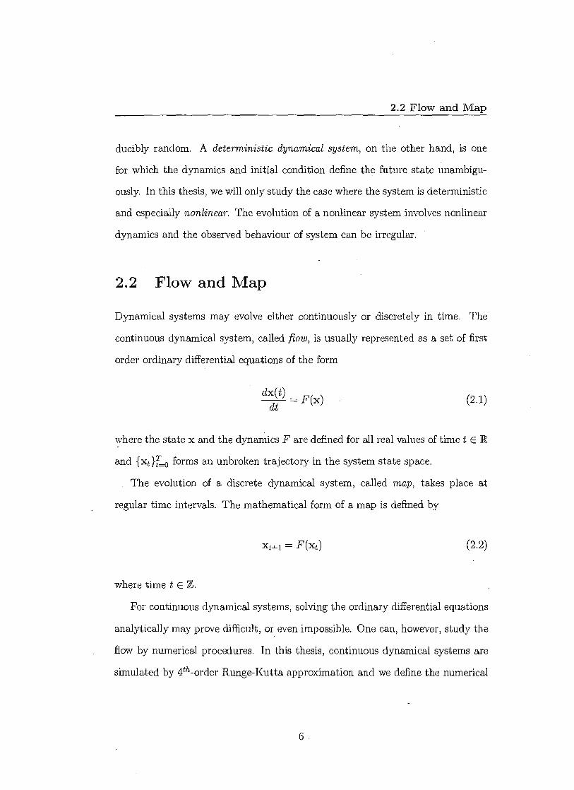
map strongly depends on the parameter value of a. Figure 2.1 shows how the
8
2.4 Analytical systems
system behaviour changes corresponding to the value of a. For a=4, a change of
....._-1 111
.„--C:7411
I
,,1
o
I ■
I
-1 fi r
1
,
1 ,IIS
1
I
I Ii.
I
q
I ii
I P I 1
1
1
-,1
I
II
$ or
1
r
I
'
1111 i
I
m..„, ,1
• 11
„
' ,!1 ;
I
1 '
, 1 II ‘1
,!„
I
1
I
ti 11 - , i HI '
,,,,,,
d .. t 1
,
I 1 III
I
II 11
r' ,
i t H
,„
t 1
1 1 11 NN I 11
i
111 .
I
3.55
3.6
3.65
3.7
3.75
3.8 3.85
3.9
3.95
4 a
Figure 2.1: The bifurcation diagram of logistic map
variables (substitute x with sin2 (7)) transforms the logistic map into the tent
map, which is proven to be chaotic (69).
The logistic map was also used as a computer random number generator by
Ulam and Neumann (1947) who studied the logistic map in its equivalent form
0.9
0.8
0.7
0.6
x 0.5
0.4
0.3
0.2
0.1
0 3.5
= 1 — axn2 . (2.4)
9

-1 5 -0.5 O 0.5 1 5
- 0.1
-0.2
- 0.3
- 0.4
2.4 Analytical systems
2.4.2 Henon map
Henon Map was introduced by Henon (40) as a simplified model of Lorenz63
model (61). The two dimensional Henon map is defined by
Xn+i = 1 — aX,L2 + Yr, (2.5)
Yrt+ 1 = bXri . (2.6)
The parameter values used in Henon (1976) were a = 1.4 and b = 0.3 in order to
produce chaotic behaviour. Figure 2.2 shows the attractor of Henon Map in the
state space.
Figure 2.2: The attractor of Henon Map
10
2.4 Analytical systems
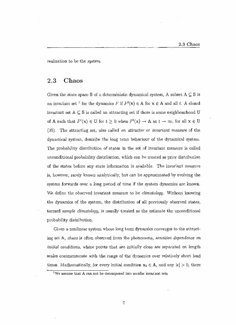
2.4.3 Ikeda map
Ikeda Map was introduced by Ikeda (45) as a model of laser pulses in an optical
cavity. With real variables it has the form
Xri+i •-y + u(Xn, cos 0 — Yri sin 0) (2.7)
Yn+1 = u(Xn sin 0 + Y„ cos 0), (2.8)
where 0 =13 — a/ (1 + Yn2 ).
With the parameter a = 6, /3 = 0.4,7 = 1, u = 0.83, the system is believed
to be chaotic. Figure 2.3 shows the attractor of Ikeda Map in the state space.
An imperfect model of Ikeda Map is obtained by replacing the trigonometric
O
0.2
0.4
0.6 0.8
1
1.2
1 .4
1 6 X
Figure 2.3: The attractor of Ikeda Map
1
0.5
O
- 0.5
- 1.5 -0 2
functions in Equation 2.7 with truncated power series (50). The truncations used
11
2.4 Analytical systems
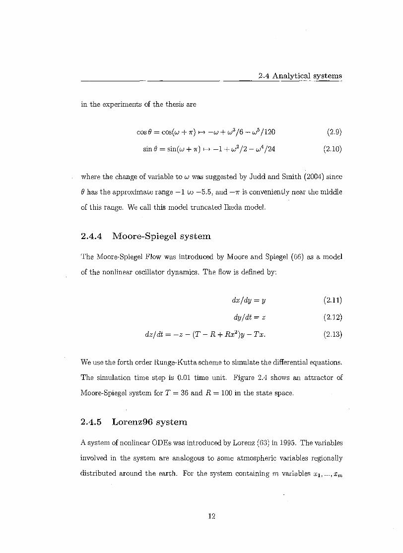
in the experiments of the thesis are
cos 0 = cos(co +701—> —co + 2/6 co 5 /120 (2.9)
sin 0 = sin(w + 7r) 1—> —1 + w2/2 w4/24 (2.10)
where the change of variable to w was suggested by Judd and Smith (2004) since
0 has the approximate range —1 to —5.5, and —7r is conveniently near the middle
of this range. We call this model truncated Ikeda model.
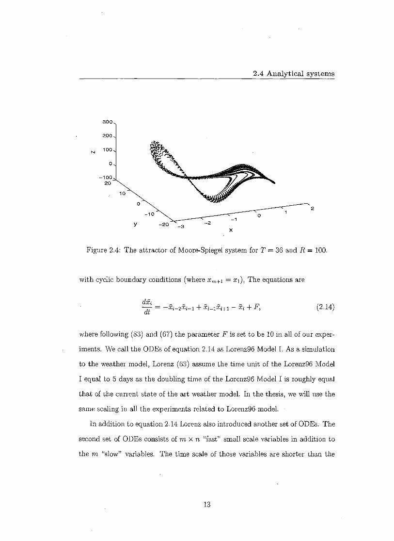
2.4.4 Moore-Spiegel system
The Moore-Spiegel Flow was introduced by Moore and Spiegel (66) as a model
of the nonlinear oscillator dynamics. The flow is defined by:
dx I dy = y (2.11)
dy I dt = z (2.12)
dz/dt = —z — (T — R + Rx 2 )y — Tx. (2.13)
We use the forth order Runge-Kutta scheme to simulate the differential equations.
The simulation time step is 0.01 time unit. Figure 2.4 shows an attractor of
Moore-Spiegel system for T = 36 and R = 100 in the state space.
2.4.5 Lorenz96 system
A system of nonlinear ODEs was introduced by Lorenz (63) in 1995. The variables
involved in the system are analogous to some atmospheric variables regionally
distributed around the earth. For the system containing m variables x l , xn,
12
= F, dt dxti
(2.14)
2.4 Analytical systems
-20 -2
x
Figure 2.4: The attractor of Moore-Spiegel system for T = 36 and R = 100.
with cyclic boundary conditions (where xn,±1 = x 1 ), The equations are
where following (83) and (67) the parameter F is set to be 10 in all of our exper-
iments. We call the ODEs of equation 2.14 as Lorenz96 Model I. As a simulation
to the weather model, Lorenz (63) assume the time unit of the Lorenz96 Model
I equal to 5 days as the doubling time of the Lorenz96 Model I is roughly equal
that of the current state of the art weather model. In the thesis, we will use the
same scaling in all the experiments related to Lorenz96 model.
In addition to equation 2.14 Lorenz also introduced another set of ODEs. The
second set of ODEs consists of m x n "fast" small scale variables in addition to
the m "slow" variables. The time scale of those variables are shorter than the
13

2.5 Nonlinear dynamics modelling
variable xi in Model I. The equations of the two sets of ODEs are
dpi ii,fz 6 1-= F
dt j=1
dyj .i hoc dt— — — -- 17:xi
Let us call the ODEs of equation 2.15 and 2.16 to be Lorenz96 Model II. The
small-scale variables yi ,i have the cyclic boundary conditions as well (that is
yn+i ,i A set of n small-scale variables are coupled to every large scale
variable. The constants b and c are set to be 10, in that case the dynamics,
represented by the small scale variables, is 10 times as fast and 1/10 as large as
that represented by the large scale variables. In the thesis the coupling coefficients
hx and hg are set to be 1. The design of Lorenz96 Model I and II is to simulate
the reality that the model is built on the m dimensional (slow dynamics) space
while the underlying system is also contain m x n fast dynamics variables which
one can not observe. In this thesis, both Lorenz96 Model I and II are simulated
by the forth order Runge-Kutta scheme with simulation time step 0.001 time
unit.
2.5 Nonlinear dynamics modelling
2.5.1 Delay reconstruction
In reality, the state of the unknown dynamical system is observed in the obser-
vation space 0. It is often the case that the observation space is not sufficient to
express the dynamics of the system unambiguously, for example, only one com-
i (2.15)
(2.16)
14

2.5 Nonlinear dynamics modelling
ponent of the system state may be measured. Rather than model in observation
space 0, it is therefore usual to reconstruct the dynamics of the system in a fur-
ther space: the model state space M. How can we construct a higher dimensional
model state space given the observation is scalar? Takens' Theorem (89) tells
us that we do not have to measure all the state space variables of the system.
We can reconstruct an equivalent dynamical system using delays of the observed
component, such method is called delay reconstruction (79; 81). Given a time
series of scalar observations, s t , t = 1, ..., n, recorded with uniform sampling time,
a trajectory of model state x t can be reconstructed in M dimensions from the
single observable s t , by delay reconstructions. This yields a series of vectors
xt = (St St —Td 7 7 St— (Al —1)Td )1
(2.17)
where Td is called the delay time. To predict a fixed period in the future, we
consider a third time scale, Tp, the prediction time. Each state x t on the trajectory
has a scalar image s t+,, and we wish to construct a predictor to determine this
image for any x.
2.5.2 Analogue models
Analogue modelling is a popular and straightforward method which is effective
to systems whose trajectories are recurrent in state space. Extracting the spatial
information of the system dynamics requires sufficient historical data to form a
learning set from which neighbours of the preimage of the state to be predicted
are defined. In this thesis the nearest neighbour is determined by the distance
between the current state and its neighbour.
15

2.5 Nonlinear dynamics modelling
• Local analogue
For local analogue, we firstly find the nearest neighbour in the model space.
We then report the nearest neighbour's image as the prediction.
• Local Random Analogue
We are not always lucky enough to determine whether or not the data from a
stochastic process or deterministic process. Paparella et al. (70) introduced
a hybrid approach, Random Analogue Prediction(RAP), which exploits the
deterministic nature of the process while incorporating variations in the
local probability distribution function, thereby adhering to the stochastic
nature of each observed trajectory. To produce the Local Random Analogue
prediction we firstly define a local neighbourhood in the model state space,
usually with a fixed radius or fixed number of k nearest neighbours. We
then select a near neighbour randomly from the k nearest neighbours and
report its image as the prediction. The probability of selecting a particular
neighbour can be based on the distance between the preimage of the state
to be predicted and that neighbour or treat the k neighbours equally.
2.5.3 Radial Basis Functions
Analogue models, when considered as a kind of local models, require constructing
a new local predictor for each initial condition by searching the learning set. As
a result, a large amount of computational resources are needed. Global models
can cover the entire domain once the model is constructed. In this section we
illustrate the Radial Basis Functions as an example of global model.
The Radial Basis Functions are a global interpolation technique. They con-
16

2.5 Nonlinear dynamics modelling
struct a predictor (map), F(x) : Ern R' which estimates the scalar observation
s for any x based on rbe centres, denoted as cj , j = 1, ..., rb, where cj E Rm. The
predictor F(x) is defined by
nc
F(x) = -0(11 x - ID, (2.18) j=1
where 0(•) are radial basis functions (14; 15; 79), II • II is the Euclidean norm.
Typical choices of radial bases functions include 0(r) = r, r 3 , and e-r2 /a where
the constant a reflects the average spacing of the centres c j . In the simplest case
the centres are chosen to cover the region of state space. To determine the value
of Aj , we assume
F(x) si . (2.19)
The Aj are then determined by solving a linear minimisation problem, i.e.
b = AA. (2.20)
, where A = [Ai , ..., Anj, A is defined by Aij — cj II) and b = [Si .••, sni ]
where n1 is the size of the learning set based on which the model is constructed (14;
15; 79).
2.5.4 Summary
In this chapter, some terminologies of dynamical system and its properties are
defined; details of the systems used in this thesis are then provided and some
17

2.5 Nonlinear dynamics modelling
relevant nonlinear dynamics modelling methods are described. Although nothing
new is presented in this chapter, the content of this chapter provide the back-
ground knowledge of the thesis.
18

Chapter 3
Nowcasting in PMS
The quality of forecasts from dynamical nonlinear models depends both on the
model and on the quality of the initial conditions. This chapter is concerned
with the identification of the current state of a nonlinear chaotic system given
both previous and current observations in the Perfect Model Scenario (PMS).
It has been shown that even under the ideal conditions of a perfect model of
a deterministic nonlinear system and infinite past observations, uncertainty in
the observations makes identification of the exact state impossible (48). Such
limitations mean that.a single "best guess" prediction is not an ideal solution to
the problem of accurate estimation of the initial state. Instead an ensemble of
initial conditions better accounts for uncertainty in the observations. Here we
define the problem of state estimation of the current state conditioned on the
past as a nowcasting problem. In the PMS, there are states that are consistent
with model's dynamics and those states that are not. Those consistent states lie
on the model's attractor. States off the model's attractor are pulled towards the
attractor. For nonlinear chaotic systems, this collapse onto the attractor dom-
19
3.1 Perfect Model Scenario
Mates the model's dynamics. Intuitively, it make sense in state estimation to
identify those states that are not only consistent with observations but also con-
sistent with the model's dynamics. The perfect model scenario is firstly defined
in Section 3.1. The theory of Indistinguishable States (IS) is then described in
Section 3.2. In Section 3.3, we introduce our methodology to address the problem
of nowcasting in PMS by first producing a reference trajectory by the method
called Indistinguishable States Gradient Descent (ISGD) and then an ensemble of
initial conditions being formed by Indistinguishable States Importance Sampler
(ISIS). Other state estimation methods including Four-dimensional Variational
Assimilation (4DVAR), Ensemble Kalman Filter (EnKF) and Perfect ensemble
are described in Section 3.4, 3.5 and 3.6 respectively. Comparison are made in
Section 3.7 i) between ISGD method and 4DVAR method relative to the reference
trajectory (defined in Section 3.3) they produce; ii) between the initial condition
ensemble generated by ISIS and that produced by EnKF; iii) between the initial
condition ensemble generated by ISIS and that of a perfect ensemble. It is the first
time that IS theory is applied to produce analysis and initial condition ensemble
and contrast with 4DVAR method and Ensemble Kalman Filter method.
3.1 Perfect Model Scenario
Let Rt EIn' to be the state of a deterministic dynamical system at time t E Z.
The evolution of the system is given by .P(Rt , : Rth IR71/ and iit+i = F(xt, a),
where F donates the system dynamics that evolves the state forward in time in
the system space R' and the system's parameters are contained in the vector
a E W.
20

3.1 Perfect Model Scenario
Define xt E IR"' to be the state of the deterministic dynamical model at time
t E Z. The model is defined by F(x t , a) : —> JR and x t+1 = F(xt , a), where
F donates the model dynamics that evolves state forward in time in the model
space Rrn and a) E W donates the model parameters.
We define the observation at time t to be s t = h(Rt ) + r/t , where is the
true state of the system. h(.) is the observation operator which projects the
state in the model space into observational space. For simplicity, we take h(.)
to be the identity. Unless otherwise stated, it is assumed that all components
of sit are observed, i.e. s t E Ie. The nt E Rth represent observational noise
(or measurement error); otherwise stated the rh are taken to be independent and
identically distributed.
In the Perfect Model Scenario(PMS), we assume i) the system state and model
states evolve according to the same structure of the dynamics, i.e. F = F. Note
that it does not require the system parameters a and the model parameters a
having the same values. In this chapter, however, we focus on the case that not
only the model class F but also the model parameters a are identical to those of
the system. ii) the system state 5 -c and the model state x share the same state
space, i.e. fit = m. iii) model state and system state correspond exactly and
iv) the noise model is independent and identically-distributed and the statistical
characteristics of the observational noise are known exactly.
The problem of nowcasting in the PMS will be interpreted as how to form
an ensemble to estimate the current state Ro given the history of observations
st , t = —N +1,..., 0, a perfect model class with perfect parameter values and the
parameters of the observational noise model.
21

3.2 Indistinguishable States
3.2 Indistinguishable States
Given a perfect model, an ideal point forecast is possible if we initialise the
model with the true state of the system. For periodical system, the state can
be identified uniquely when t —co. For chaotic systems, noisy observations
prevent us from identifying the true state of the system precisely, nonetheless
one can find a set of states that are indistinguishable from the true state given
the perfect model and the noise model (48). In this section we describe the
background knowledge of Indistinguishable States Theory following the work of
Judd and Smith in (48). Figure 3.1 (reproduced from Figure 1 in (48)) shows
Figure 3.1: Following Judd and Smith (2001), Suppose xt is the true state of the system and yt some other state where x t and yt E R2 . The circles centred on xt and yt represent the bounded measurement error. When an observation falls in the overlap of the two circles (e.g., at a), then the states xt and yt are indistinguishable given this single observation. If the observation falls in the region about xt , but outside the overlap region (e.g., at /3), then on the basis of this observation one can reject y t being the true state, i.e., x t and yt are distinguishable given the observation.
22

3.2 Indistinguishable States
that based on one single observation s t of state xt , there exist many states y t each
of which is indistinguishable from xt because of the observational uncertainty if
the overlap region in Figure 3.1 covers the observation s t . Notice that given the
bounded noise model, xt and yt are indistinguishable as there exist the overlap
region in Figure 3.1. However, a particular realization of observation, e.g. /3 in
Figure 3.1, could distinguish xt from yt .
We describe the statistical background of Indistinguishable State Theory in
the following. For the convenience of explanation, x t , yt and st are scalars. Let
the probability density function of the observational noise be p(•), the joint prob-
ability density of xt and yt being indistinguishable is then defined by
f P(st — xt)P(st — yt )dst . (3.1)
This joint density function depends only on the difference between xt and y t and
the distribution of the measurement error s t — xt , since
f gst — xt)P(st — Yt)dst = P(st — xt)P(st xt + xt — Yt)d(st xt), (3.2)
The indistinguishability of two states x t and yt can be quantified by the normalised
density function
f p(st — xt )p(st — xt + yt)d(st xt) q(xt — yt ) — f p(st — xt)p(st — xt)d(st — xt)
(3.3)
23
3.2 Indistinguishable States
This function is called q density. The normalisation implies the constraint that
when xt = yt , the density function reaches its maximum value of 1: in no case
that xt is distinguishable from itself. If q(xt — yt ) = 0, then the states xt and yt
are distinguishable with probability one, any particular realization of observation
will only be consistent with either xt or yt but not both. A value q(x t — yt ) > 0
indicates that x t and yt are indistinguishable given the noise model. One should
notice that there might be some particular observations that can distinguish xt
from yt for example, in the bounded noise case, if )3 in Figure 3.1 is observed
xt and yt are distinguishable. Therefore particular realizations will give extra
information to distinguish x t and yt besides the q density.
Such q density can be generalised to a sequence of observations. Any system
state xo defines a trajectory (we will often drop the subscript for x 0 afterwards),
that goes infinite past and terminates at x. Given a time series of observations
st , t = 0, —1, —2, ..., it follows from the independence of the measurement error
that by considering all the states on the trajectory, the indistinguishability of two
state x and y is then given by the product
Q(x, y) = fl q(xt - t<0
(3.4)
Similar to the single observation case, If Q(x, y) > 0, then the trajectory ending
at x and the trajectory ending at y are not distinguishable, given the noise model.
Therefore the set of indistinguishable states of x is defined as
111(x) = {y E : Q(x,y) > 01. (3.5)
24
3.3 Nowcasting using indistinguishable states
As showed in (48), for three typical measurement error densities p(.) (Gaussian
error density, Uniform error and non-uniform bounded error), IHI(x) is non-trivial
and is a subset of the unstable set of x. In practice, only finite observations are
available. The Q density used in the later application is calculated within a finite
time interval. This requires a reference trajectory as discussed in Section 3.3.1.
3.3 Nowcasting using indistinguishable states
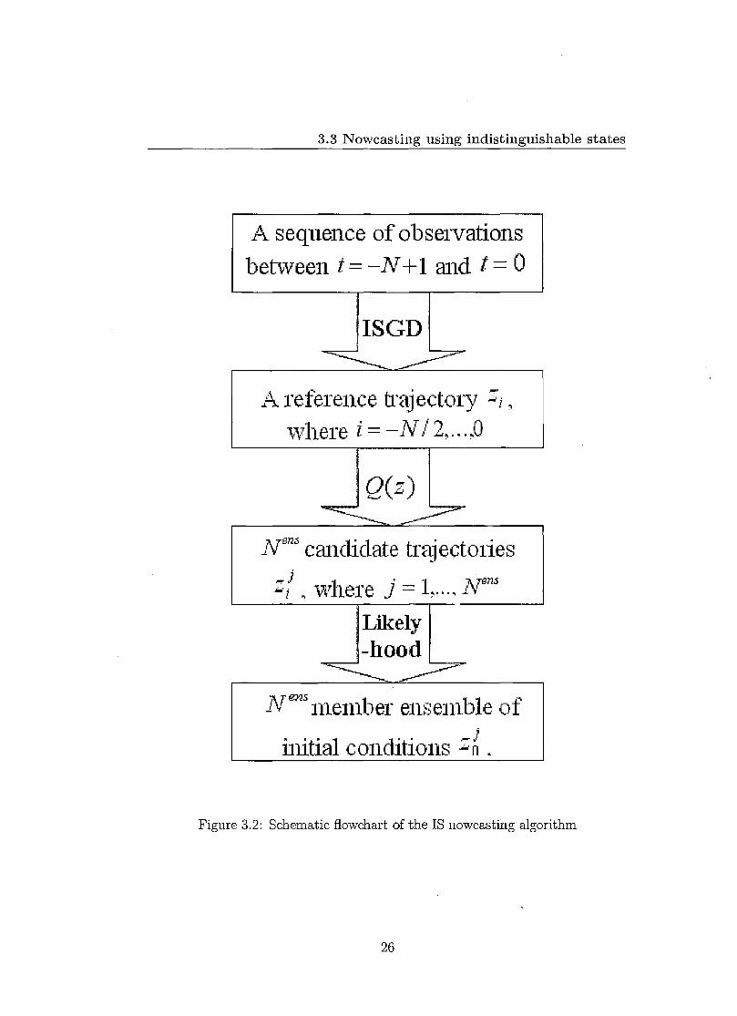
In this section we introduce a new methodology to address the problem of now-
casting in the perfect model scenario by applying the Indistinguishable States (IS)
theory. An illustration of this methodology is depicted in the schematic flowchart
of Figure 3.2.
Given a sequence of observations, we firstly identify a trajectory of the model,
here termed a reference trajectory' in order to apply the IS theory to form an
ensemble of initial conditions: The reference trajectory is discussed in detail in
Section 3.3.1. The Indistinguishable States Gradient Descent (ISGD) (48) method
is suggested to find the reference trajectory. Based on the reference trajectory,
we introduce a method called Indistinguishable States Importance Sampler (ISIS)
to form an Nees member ensemble of initial conditions (details are discussed in
Section 3.3.3). The ISIS method includes two procedures, i) draw Nees candidate
trajectories from the set of indistinguishable states of the reference trajectory
according to Q density; ii) use the end point of each candidate trajectories as the
ensemble member of the estimation of current state and weight them according
to the likelihood of the observations.
'In practice particular model trajectory chosen to be the reference trajectory will depend on the details of algorithm.
25
A reference trajectory where I = —NI 2,...,0
Q(z)
N's candidate trajectories • where j = Ar"
3.3 Nowcasting using indistinguishable states
A sequence of observations between t = —N+1 and t = 0
ISGD
Are''''s member ensemble of initial conditions -1 1=
Figure 3.2: Schematic flowchart of the IS nowcasting algorithm
26
3.3 Nowcasting using indistinguishable states
3.3.1 Reference trajectory
In our nowcasting methods, we define a reference trajectory to be the analysis
about which an ensemble can be formed. Generally, any model trajectory might
be a reference trajectory. The quality of the ensemble depends largely on how
"good" the reference trajectory is 1 .
In the PMS, as we discussed in Section 3.2, there is a set of indistinguishable
states of the true state, i.e. H(ii). Let the reference trajectory end at x. One
can form an ensemble of initial condition by drawing members from the set of
indistinguishable states of the model state x, i.e. II-1[(x). It is desired that such set
of indistinguishable states IHI(x) contains the true state x , which means Q(51, x) >
0. And symmetrically the model state x is in the set of indistinguishable states
of true state Elf(*) 2 . Therefore the desirable reference trajectory we are looking
for acts as a proxy of the true state.
We suggest using the Indistinguishable States Gradient Descent(ISGD) method (48)
to find a reference trajectory which use the information both from model dy-
namics and the observations (details are discussed in the following section). In
practice, the set of indistinguishable states of the reference trajectory we obtain
by ISGD method, almost surely, does not contain the true state, nor would any
other methods due to the fact that only finite sample is available. We are, how-
ever, interested in whether the reference trajectory we obtain provides a better
ensemble of estimates of current states.
'or "are". We might take more than one reference trajectory in future work 2 1t does not mean that the set of indistinguishable states of the true state and that of the
reference trajectory are identical but overlapped
27

3.3 Nowcasting using indistinguishable states
3.3.2 Finding a reference trajectory via ISGD
Given a sequence of observations and a perfect model, we apply Indistinguishable
States Gradient Descent algorithm (48) to find a reference trajectory. Judd and
Smith (2001) demonstrate that the states produced by the ISGD method reflect
the set of indistinguishable states of the true state. Here we give a brief introduc-
tion of how to apply such method (see (18) for more details). Let the dimension
of our model state space be m and the number of observations be n; the sequence
space is an m x n dimensional space in which a single point can be thought of as a
particular series of n states u i , i = —n+ 1, .., 0. Some points in sequence space are
trajectories of the model, some are not. We define a pseudo-orbit to be a sequence
of model states that at each step differ from trajectories of the model, that is,
ui+1 F(u i )). Particularly the observations being points of interest which, with
probability one, are not a trajectory but a pseudo-orbit. We define the mismatch
to be:
F(ui)
(3.6)
Model trajectories with probability 1 have e i = 0. We apply a gradient
descent (GD) algorithm (details of GD can be found in appendix), initialised at
the observations, i.e. u i = s t , and evolving the GD algorithm so as to minimise
the sum of the squared mismatch errors. It has been proven (18) that the cost
function
C(u) = (3.7)
28

3.3 Nowcasting using indistinguishable states
has no local minima, while at points along every segment of trajectory the cost
function has the value of zero. As the minimisation runs deeper and deeper,
the pseudo-orbit u_n+1, ••-, uo is closer to be a trajectory of the model. In other
words, the GD algorithm takes us from the observations towards a model tra-
jectory. In practice, the GD algorithm is run for a finite time and thus not a
trajectory but a pseudo-orbit is obtained. We denote the pseudo-orbit obtained
from finite GD runs as yi , i = —n + 1, ..., 0. In order to find our reference trajec-
tory close to the pseudo-orbit obtained from GD algorithm, we iterate the middle
point y-7,12 1 forward to create a segment of model trajectory zi , i = —n/2, ...,
(y—n/2 z_n/2 ). We treat such model trajectory to be the reference trajectory,
in Meteorology this trajectory might be called "the analysis". It is important to
notice that although the GD algorithm can be applied to any length of obser-
vation window, the reference trajectory will likely diverge from the pseudo-orbit
when n is large due to the consequence of sensitivity to initial conditions. In the
results shown in section 3.7, n is adjusted to provide the reference trajectory that
is close to the pseudo-orbit yi .
3.3.3 Form the ensemble via ISIS
In a fully Bayesian treatment one could use the natural measure as a prior and
then update given the observations and the inverse noise model. Inasmuch as
natural measure cannot be phrased analytically, in general, this approach is com-
putationally intractable due to the cost of estimating the prior. The idea of ISIS
is to select the ensemble members using the set of Indistinguishable States of the
reference trajectory as an importance sampler (53). In order to do this, we firstly
lif n is odd, we take 3, ( - 7.0_ 1)/2
29

3.3 Nowcasting using indistinguishable states
generate a large number of model trajectories, called candidate trajectories, from
Which ensemble members can be selected. Ensemble members are drawn from
the candidate trajectories according to their Q density relative to the reference
trajectory. There are many ways to produce candidate trajectories. Here we
suggest two methods of producing candidate trajectories. i) Sample the local
space around the reference trajectory. One can perturb the starting point of the
reference trajectory and iterate the perturbed point forward to create candidate
trajectories. ii) Perturb the whole segment of observations s i , i = —n+ 1, ..., 0 and
apply the ISGD onto the perturbed orbit to produce the candidate trajectories,
i.e. the same way that we produce the reference trajectory. Although method ii)
may produce more informative candidates, it is obviously much more expensive
than method i) since the ISGD involves a large number of model runs. The re-
sults shown in section 3.7 are produced by using method i) to generate candidate
trajectories.
Given Ncand number of candidate trajectories, the Q density is then used to
measure the indistinguishability between the candidate trajectories and reference
trajectory. Since only a segment of reference trajectory is obtained, the Q density
is calculated over the time interval (- 722:, 0).
To form an Nens member ensemble estimate of current state, we randomly
draw IV ens trajectories from Neared candidate trajectories according to their Q
density, i.e. the larger its Q density is, the more likely the candidate trajectory
is chosen. And the end point of each selected candidate trajectory is treated as
the ensemble member. As the Q density depends not on the observations but
on the noise model, in order to take account of the information in the particular
observations we have, we weight the ensemble members using the likelihood of
30

3.3 Nowcasting using indistinguishable states
the observations over the time interval (- 12-1 , 0). The likelihood function is given
by:
1 0
L(z3 ) = -9 (z .7 - s yr-1.(zit St ), t t (3.8) = — 2
where j E {1, ..., Nens} 1r1 — 1. 1 is the inverse of the covariance matrix of the obser-
vational noise, zi denotes the chosen candidate trajectory and zio is then taken
to be the j ih member of the ensemble estimates of the current state.
3.3.4 Summary
In this section, a new state estimation method based on applying IS theory is in-
troduced in the perfect model scenario. A reference trajectory, which is expected
to reflect the set of indistinguishable states of the true state, is identified by ISGD
algorithm. Based on the reference trajectory (analysis), the ISIS method is then
introduced to form ensemble members from model trajectories, therefore the en-
semble members reflect the nonlinearity of the dynamics. Our methodology is
aiming to enhance balance between the extracting information from the dynamic
equations and information in the observations. Two state-of-the-art methods,
Four-dimensional Variational Assimilation and Ensemble Kalman Filter, are dis-
cussed in the following sections. Results shown in Section :3.7 demonstrate that
our method outperforms those two methods. The Perfect Ensemble as the opti-
mal ensemble states is defined and discussed in Section 3.6. Comparison between
the Perfect Ensemble and our method is provide in Section 3.7.
31
3.4 4DVAR
3.4 4DVAR
Four-dimensional Variational Assimilation (4DVAR) is a widely used method of
noise reduction in data assimilation (18; 19; 90). The method provides an es-
timate of a system state by using the information in both model dynamics and
observations. 4DVAR looks for initial conditions that are consistent with the sys-
tem trajectory by taking account the observational uncertainty of the sequence
of system observations. It aims to select the initial condition which minimises
a cost function which measures the misfit between the model states and obser-
vations. During the application of 4DVAR, the minimisation is carried out over
short assimilation windows rather than across all available data (Increasing the
window length will not only increase the CPU cost but also introduce problems
due to local minima (65; 71)).
3.4.1 Methodology
Assume the observations recorded within a time interval t E (-n, 0) will be used.
Let xt = F(xt_ i ), the 4DVAR cost function is:
Cldvar —2(x, — xb n )TB1( —n x n — xb
—n ) (3.9)
1 2
(H(xt) — st)Tr -1 (1/(xt) — St), t=—n
where x_„ is the model initial condition, xb , is the first guess, or background state
of the model and 13.7„1 is a weighting matrix that is the inverse of the covariance
matrix of xb. The first term in the cost function is usually called the background
32

3.4 4DVAR
term. s t is the observation at time t and P -1 is the inverse of the covariance
matrix of the observational noise. Hence the second term in the cost function
minimises the distance between the model trajectory and the observations.
By locating a minimum of the cost function, one finds initial conditions which
defines a model trajectory that has the minimum distance from the observations.
Such model trajectory is expected to be found in the perfect model case and
the longer window is looked at, the better the global minima is expected to.
In practice, increasing the window length will also increase the density of local
minima which makes it much harder to locate the global minima (65; 71).
3.4.2 Differences between ISGD and 4DVAR
The 4DVAR method aims to produce a model trajectory consistent with obser-
vations. The 4DVAR analysis, whatever it may be in practice, can also be used
as a reference trajectory to form an initial condition ensemble by ISIS. Although
both ISGD method and 4DVAR method use the information of both model dy-
namics and observations to produce the model trajectories, there are fundamental
differences between them.
• Both methods produce the model trajectories "close" to the observations
but in a different way. The 4DVAR method tends to find a model trajec-
tory close to the observations as the cost function minimises the distance
between the model trajectory and the observations. If one initialises the
cost function with the true state of the system, the minimisation algorithm
will with probability 1 move away from the trajectory in order to minimise
the distance between observations and the model trajectory. Only if the
33
3.4 4DVAR
window is infinite then this does not have to happen. In practice 4DVAR
is applied to an assimilation window with finite length, the cost function
forces the resulting model trajectory to be close to the observations, which
may cause the estimate stay further away from the true state.
In the ISGD algorithm, the cost function itself does not contain any con-
straints to force the result staying close to the observations. The GD min-
imisation is, however, initialised with the observations in practice 1 . The
states one achieves is on the attracting manifold that is close to the observa-
tions (48; 52). Unlike 4DVAR method, ISGD method does not require the
pseudo-orbit to stay close to the observations and actually ISGD method
forces the pseudo-orbit, on average, to move away from the observations as
the minimisation goes further and further.
The results shown in section 3.7.1, indicate that 4DVAR method tends to
produce the model trajectory closer to the observations than ISGD method.
• The behaviour of the 4DVAR cost function strongly depends on the as-
similation window while ISGD does not. In practice, the number of local
minima in the 4DVAR cost function increases with the length of the data
assimilation window (71). The model trajectory defined by the local min-
ima stays father away from the observations than the one defined by the
global minima of the cost function. The results trapped in the local minima
are very likely inconsistent with the observations. Gauthier(1992), Stensrud
and Bao (1992) and Miller et al. (1994) have performed the 4DVAR ex-
periments with Lorenz63 system (61). They all found that performance of
l One may initialise the GD minimisation with better analysis if it is available
34

3.4 4DVAR
assimilation varies significantly depending on the length of the assimilation
window and difficulties arises with the extension of assimilation window due
to the occurrence of multiple minima in the cost function. Applying the
4DVAR algorithm, one faces the dilemma of either from the difficulties of
locating the global minima with long assimilation window or from losing
information of model dynamics and observations by using short window.
The mismatch cost function in ISGD does not introduce such shortcomings.
Although the cost function itself has more than one minima, each minima
represents model trajectories where the mismatch cost function equals zero.
Longer assimilation windows do not bring any trouble to the minimisation
algorithm using GD. On the other hand, as longer assimilation window con-
tains more information of the model dynamics and observations, the results
in Section 3.7 show that the states obtained by ISGD method stay closer to
the true state when the window length increases. The minima of the cost
function are only model trajectories. And by initialising the minimisation
algorithm with the observations, a pseudo-orbit on the attracting manifold
which close to the observations can be found.
• The aim of 4DVAR is to locate a model trajectory through the available
observations which minimises the distances between model states and ob-
servations, which is the second term of the cost function. The first term of
the cost function, i.e. the background term, contains xb, the estimation of
the state at the initial time of the assimilation window. In practice xb can
be obtained from the previous assimilation window. By having the back-
ground term in the cost function, it not only makes the minimisation faster
35

3.5 Ensemble Kalman Filter
but most importantly tries to help the minimisation algorithm avoid being
trapped from the local minima. In the presence of multiple minima, the
result of the minimisation will depend on the starting point of the minimi-
sation (71). When the window length is very long, the second term of the
cost function dominates the cost function. But when- the window length is
short, the background term forces the final estimate to stay close to the ini-
tial estimate, which means the quality of the assimilation depends critically
on the initial estimate. While the ISGD method does not have to use any
other initial estimates except the observation itself as the minimisation is
initialised with the entire window of observations.
In the sense of forming the ensemble, we can also treat the model trajectory
produced by 4DVAR as a reference trajectory and form the ensemble in the same
way as ISIS method. Obviously the quality of the ensemble depends strongly on
the quality of the reference trajectory. In section 3.7.1, we compare the quality
of the model trajectory produced by 4DVAR and the one generated by ISGD in
both low dimensional and higher dimensional case. The results show that the
reference trajectory produced by ISGD is more consistent with the observations
and closer to the true system trajectory than the 4DVAR results.
3.5 Ensemble Kalman Filter
Second well established class of algorithms has been defined for state estimation
are sequential algorithms. In sequential algorithms, one integrates the model
forward until the time that observations are available, the state at that time
estimated by the model is usually called the first-guess, which is then corrected
36

3.5 Ensemble Kalman Filter
with the new observations. The sequential algorithm, used in this chapter to
compare with our methods, is based on the forms of Kalman filter (54). Although
we only provide the comparison between ISIS method and a state of the art
ensemble Kalman filter scheme (1; 2) later in the chapter, we first provide a brief
overview of other versions of Kalman Filter methods including Kalman filter,
Extended Kalman filter as background information on the ensemble Kalman filter
being discussed later.
3.5.1 Kalman Filter
The Kalman filter (54) is a commonly used method of state estimation (86). It
provides a sequential method to estimate the state of a system, with the aim of
minimising the mean of the squared error of one step forecast. It gives the optimal
estimate when the system dynamics are linear and the model is perfect (86).
The Kalman filter addresses the general problem of trying to estimate the
state of the system xt E Rin, where the dynamics of the system is F:
xt = fr (Xt-1)
(3.10)
• Given a linear model F:
F(xt ) = Axt, (3.11)
where the model F need not be a perfect representation of the system's
37

3.5 Ensemble Kalman Filter
dynamics F. It is assumed that model space and system space are identical.
Any discrepancy between the model and the system can be written as:
P(xt ) = F(xt ) + wr t (3.12)
where 7XI is understood to reflect the model error. When defining the
Kalman Filter it is also assumed that Tx; is IID normally distributed with
zero mean and variance Q err
• given observations s E Rmobs we have
St = h(xt) + Et (3.13)
where ct is the observational noise, assumed to be IID normally distributed
with zero mean and variance F. The function h is the observation function,
here assumed to be linear: h(xt ) = Hxt . The in,°b5 x m matrix H is
a projection operator that gives the transformation from model space to
observation space.
We define xb E to be the background or prior estimate of the system state
at time t, and 4 E Rm to be the analysis or a posteriori estimate of the system
state xt . The estimation error is then defined by
38
3.5 Ensemble Kalman Filter
et = xt — xtb ,
ect' = xt —
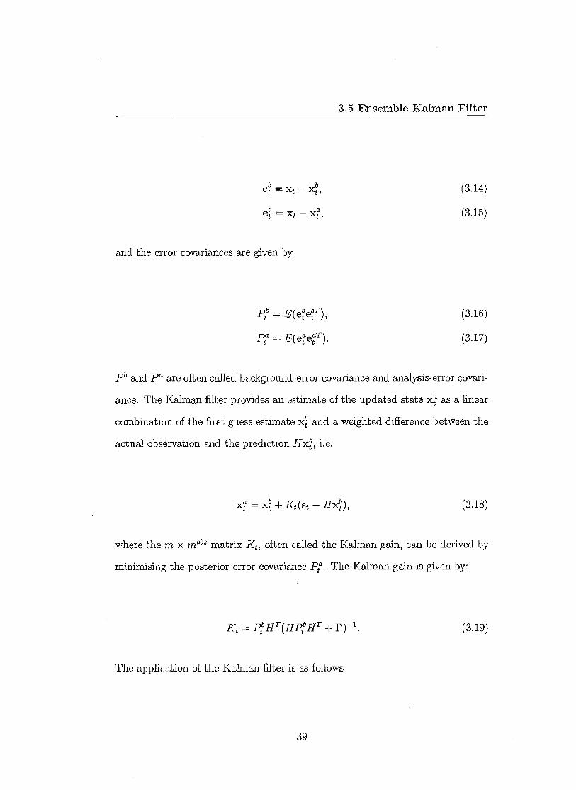
and the error covariances are given by
(3.14)
(3.15)
Pt b E (etbetbT) , (3.16)
Pa E(eaetaT). (3.17)
Pb and Pa are often called background-error covariance and analysis-error covari-
ance. The Kalman filter provides an estimate of the updated state 4 as a linear
combination of the first guess estimate xt and a weighted difference between the
actual observation and the prediction H4, i.e.
xa + Kt (s, — rixtt'), (3.18)
where the m x m°b5 matrix Kt , often called the Kalman gain, can be derived by
minimising the posterior error covariance P. The Kalman gain is given by:
Kt = ppliT(Hp:HT +11) -1 . (3.19)
The application of the Kalman filter is as follows
39
3.5 Ensemble Kalman Filter
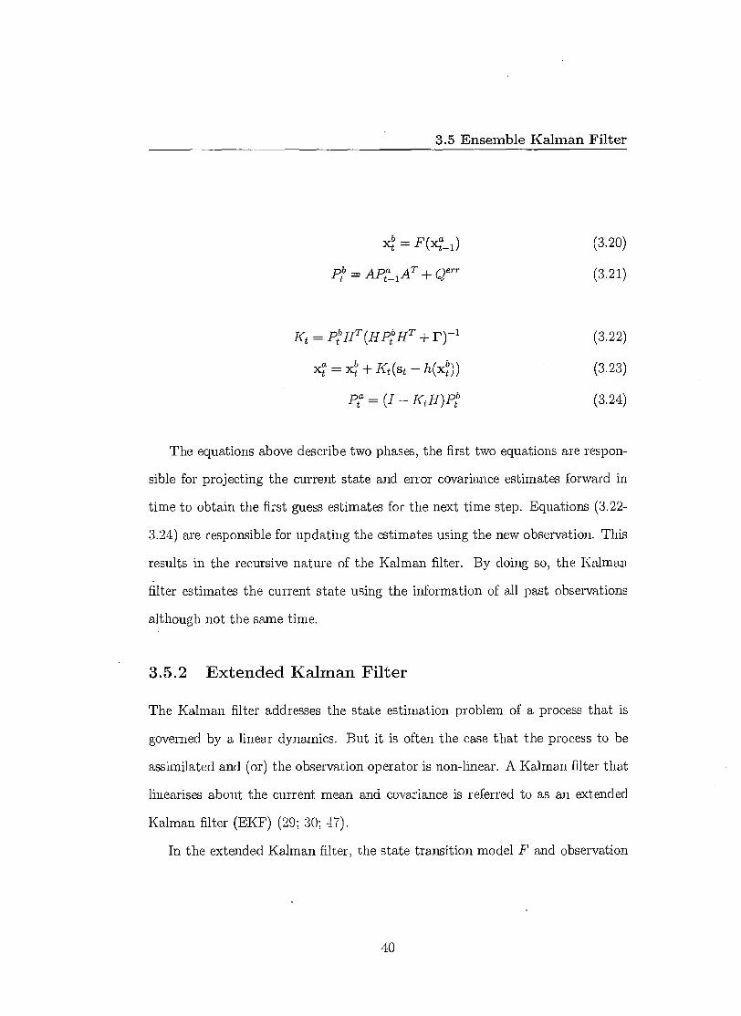
xeb = F (4-1) (3.20)
Pb Apta, 1 AT err (3.21)
Kt = Pb HT (H Ptb HT + r) -1 (3.22)
= x:+Kt (s t — h(4)) (3.23)
Pt = (1 KtH)ptb (3.24)
The equations above describe two phases, the first two equations are respon-
sible for projecting the current state and error covariance estimates forward in
time to obtain the first guess estimates for the next time step. Equations (3.22-
3.24) are responsible for updating the estimates using the new observation. This
results in the recursive nature of the Kalman filter. By doing so, the Kalman
filter estimates the current state using the information of all past observations
although not the same time.
3.5.2 Extended Kalman Filter
The Kalman filter addresses the state estimation problem of a process that is
governed by a linear dynamics. But it is often the case that the process to be
assimilated and (or) the observation operator is non-linear. A Kalman filter that
linearises about the current mean and covariance is referred to as an extended
Kalman filter (EKF) (29; 30; 47).
In the extended Kalman filter, the state transition model F and observation
40

3.5 Ensemble Kalman Filter
model h need not be linear functions of the state. It is, however, assumed that
these functions are differentiable.
The equations of EKF differs from KF in that H represents the mobs x m
Jacobian matrix of h: H = ---°h instead of the linear projection operator and A ox
is the m x m Jacobian matrix of model F: A = a often referred to as the x
transition matrix.
Similar to the Kalman filter, model errors are required to be uncorrelated
with the growth of analysis errors through the model dynamics. This becomes
a fundamental flaw of EKF as the distributions of the initial uncertainty are no
longer normal after going through the nonlinear model. The linear assumption
of error growth in EKF results in an overestimate of background error variance.
Furthermore, estimating the model error covariance Q err may be particularly
difficult while the accuracy of the assimilation strongly depends on Q"T (37).
3.5.3 Ensemble Kalman Filter
The ensemble Kalman filter (EnKF) was first introduced by Evensen (23) as a
method for avoiding the expensive calculation of the forecast error covariance
matrix necessary for both KF and EKF in Numerical Weather Prediction. The
mechanism of the EnKF's production of an analysis follows from the methods of
the KF and EKF. It differs only in its method of using an ensemble to estimate
the forecast error covariance matrix. No assumptions about linearity of error
growth are made.
There are two general classes of ensemble Kalman filter, stochastic (37; 41;
42; 43) and deterministic (1; 7). Both filters propagate the ensemble of analyses
41

1 P =
Nens (3.26)
3.5 Ensemble Kalman Filter
with non-linear models, the primary difference is whether or not random noise is
applied during the update step to simulate observational uncertainty (37).
Let X = ..., xre') be an /Yens member ensemble state estimation at time
t. The ensemble mean X is defined as
= N'ns
1 r1 (3.25)
IVens
i=1
and the variance P of a finite ensemble is given:
The EnKF uses the variance of nonlinear ensemble forecast P to estimate the
background-error covariance P b
• Stochastic update methodology
The traditional ensemble Kalman filter (37; 41; 42; 43) involves a stochastic
update method. This algorithm updates each member according to differ-
ent perturbed observations. As the perturbation involves randomness, the
update is considered stochastic method.
We define the perturbed observations "S i = s + m where 7ji N N(0, r).
For each ensemble member x it the update equations are:
42

3.5 Ensemble Kalman Filter
+ k(si — h(4))
(3.27)
k = Pb HT (H Pb HT + F) -1
(3.28)
As we can see from the equation, the perturbed observations are used to
update the ensemble states, similar to the Kalman gain K in EKF (10), but
using the ensemble to estimate the background-error covariance matrix.
If unperturbed observations are used in (15) without other modifications
to the algorithm, the analysis error variance Pa will be underestimated,
and observations will not be adequately weighted by the Kalman gain in
subsequent assimilation cycles (37). Adding noise to the observations in
the EnKF can, however, introduce spurious observation background error
correlations that can bias the analysis-error covariances, especially when
the ensemble size is small (92). Such shortage is overcome by deterministic
update methodology.
• Deterministic update methodology
Deterministic algorithm like (1; 7) update in a way that generates the same
analysis error covariance without adding stochastic noise. There are a num-
ber of different approaches, here in the case we are only going to talk about
one. Here we briefly describe one of the methods called the ensemble square-
root filter(EnSRF) (92) which is mathematically equivalent to the Ensemble
Adjustment Kalman filter (1). We use this method to produce ensemble
results comparing with the results obtained from IS method in Section 3.7.
43
3.6 Perfect Ensemble
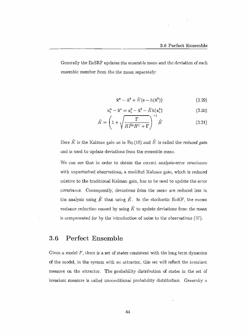
Generally the EnSRF updates the ensemble mean and the deviation of each
ensemble member from the the mean separately:
Ra =Xb k(S — h(5Cb ))
- = )4, - )cb - kh(x)
(3.29)
(3.30)
(3.31) k= HPb.riT +r
) (1+
Here k is the Kalman gain as in Eq.(16) and k is called the reduced gain
and is used to update deviations from the ensemble mean.
We can see that in order to obtain the correct analysis-error covariance
with unperturbed observations, a modified Kalman gain, which is reduced
relative to the traditional Kalman gain, has to be used to update the error
covariance. Consequently, deviations from the mean are reduced less in
the analysis using K than using K. In the stochastic EnKF, the excess
variance reduction caused by using K to update deviations from the mean
is compensated for by the introduction of noise to the observations (37).
3.6 Perfect Ensemble
Given a model F, there is a set of states consistent with the long term dynamics
of the model, in the system with an attractor, this set will reflect the invariant
measure on the attractor. The probability distribution of states in the set of
invariant measure is called unconditional probability distribution. Generally a
44
3.6 Perfect Ensemble
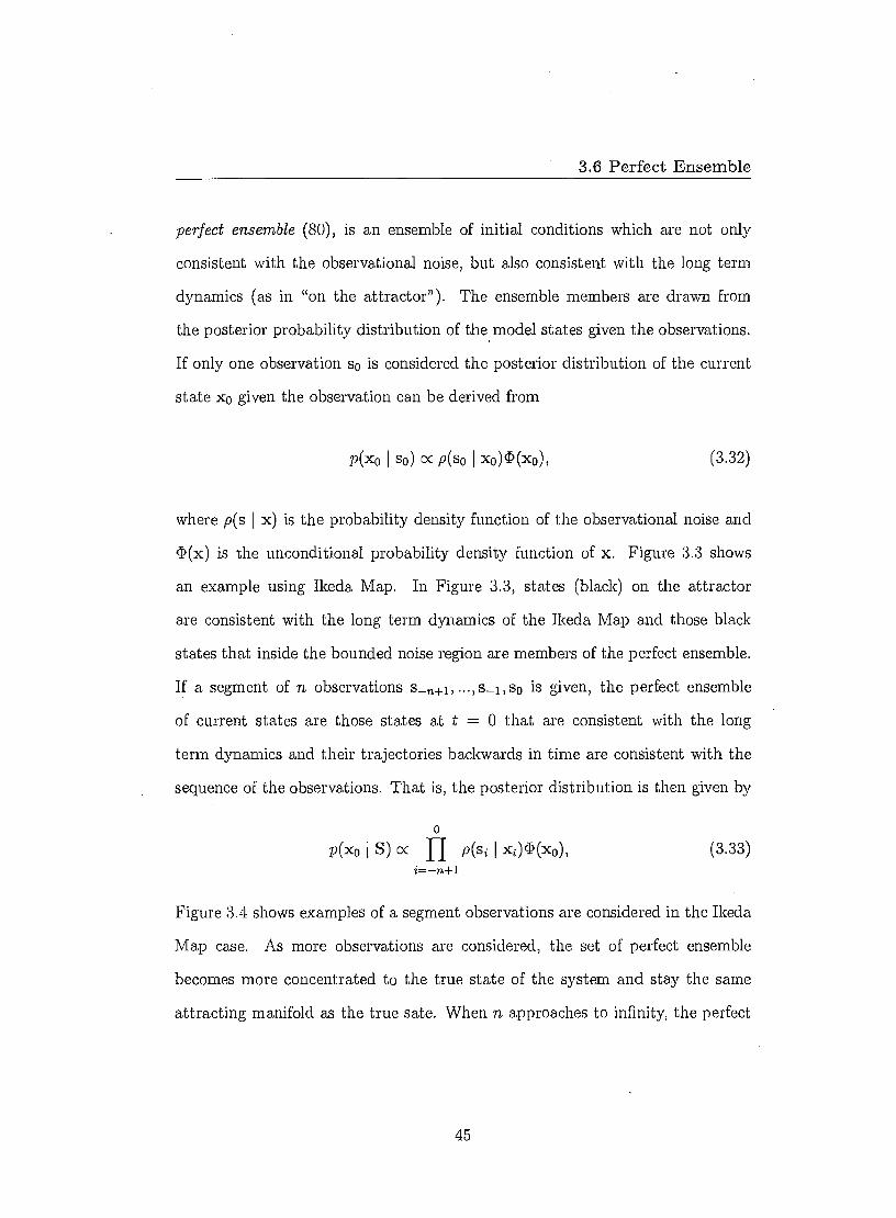
perfect ensemble (SO), is an ensemble of initial conditions which are not only
consistent with the observational noise, but also consistent with the long term
dynamics (as in "on the attractor"). The ensemble members are drawn from
the posterior probability distribution of the model states given the observations.
If only one observation so is considered the posterior distribution of the current
state xo given the observation can be derived from
p(xo I so) a p(so xo) 1 (xo), (3.32)
where p(s x) is the probability density function of the observational noise and
41)(x) is the unconditional probability density function of x. Figure 3.3 shows
an example using Ikeda Map. In Figure 3.3, states (black) on the attractor
are consistent with the long term dynamics of the Ikeda Map and those black
states that inside the bounded noise region are members of the perfect ensemble.
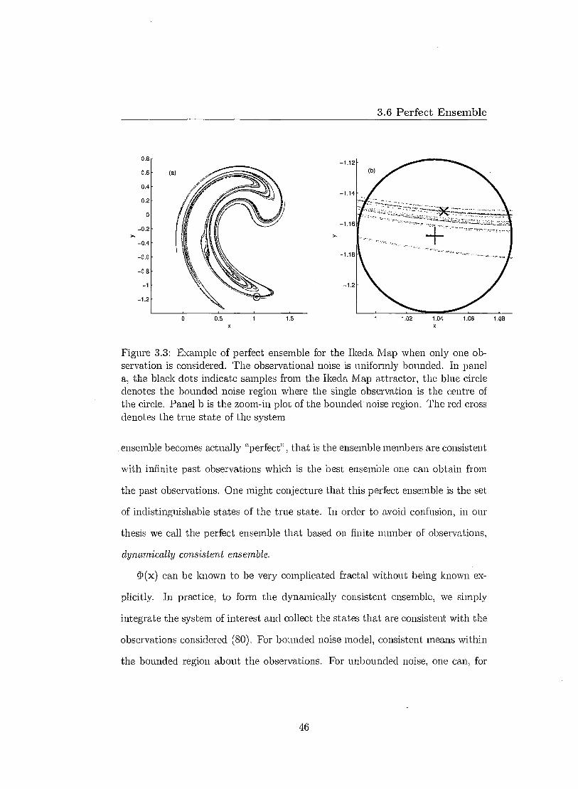
If a segment of n observations s_ n+i , s_ 1 , so is given, the perfect ensemble
of current states are those states at t = 0 that are consistent with the long
term dynamics and their trajectories backwards in time are consistent with the
sequence of the observations. That is, the posterior distribution is then given by
p (xo S) oc p (si I xi ) (I) (x0 ) , (3.33)
Figure 3.4 shows examples of a segment observations are considered in the Ikeda
Map case. As more observations are considered, the set of perfect ensemble
becomes more concentrated to the true state of the system and stay the same
attracting manifold as the true sate. When n approaches to infinity, the perfect
45
0 0.5 1.5
0
-0.2
-0.4
-0.6
-0.8
-1.2
- 1.12
-1.14
-1.16
- 1.18
-1.2
3.6 Perfect Ensemble
Figure 3.3: Example of perfect ensemble for the Ikeda Map when only one ob-servation is considered. The observational noise is uniformly bounded. In panel a, the black dots indicate samples from the Ikeda Map attractor, the blue circle denotes the bounded noise region where the single observation is the centre of the circle. Panel b is the zoom-in plot of the bounded - noise region. The red cross denotes the true state of the system
ensemble becomes actually "perfect" , that is the ensemble members are consistent
with infinite past observations which is the best ensemble one can obtain from
the past observations. One might conjecture that this perfect ensemble is the set
of indistinguishable states of the true state. In order to avoid confusion, in our
thesis we call the perfect ensemble that based on finite number of observations,
dynamically consistent ensemble.
(I)(x) can be known to be very complicated fractal without being known ex-
plicitly. In practice, to form the dynamically consistent ensemble, we simply
integrate the system of interest and collect the states that are consistent with the
observations considered (80). For bounded noise model, consistent means within
the bounded region about the observations. For unbounded noise, one can, for
46
-1.12
- 1.14
-1.16
-1.18
- 1.2
1.02 1.04 X
1,06 1.08
- 1.12
- 1.14
- 1.18
- 1.2
1.02 1.04 1.06 1.08
- 1.12
-1.14
- 1.18
-1.2
-1.12
- 1.14
- 1.18
-1.2
3.6 Perfect Ensemble
Figure 3.4: Following Figure 3.3, examples of perfect ensemble are shown for the Ikeda Map when more than one observation is considered. The perfect ensem-ble of different number observations are considered are plotted separately. Two observations are considered in panel (a), 4 in panel (b), 6 in panel (c) and 8 in panel (d). In all the panels, the green dots are indicates the members of perfect ensemble.
example, define consistent to be within the sphere centered on the observation.
The radius of the sphere should be chosen depending on the number of obser-
47

3.7 Results
vations, to increase as the number of observations increases. In practice we use
`within four standard deviations' (39) i.e. the states, treated to be consistent with
observations, never farther than 4a from the observations. Although the dynam-
ically consistent ensemble produce a desirable ensemble state of the current state
where the ensemble members are consistent with both model dynamics and the
observations, it is extremely costly to construct such ensemble, when the model
states are in the high dimensional state space. Even in low dimensional systems,
it is prohibitively costly when a relative long observation window is considered.
3.7 Results
In this section we first compare the ISGD method with 4DVAR method by looking
at the model trajectory each produces. We then compare the ISIS method with
Ensemble Kalman Filter by comparing ensemble members in the state space and
evaluating them using the new e-ball method defined in Section 3.7.2. Finally we
compare our met hod with the perfect ensemble.
3.7.1 IS GD vs 4DVAR
Since the 4DVAR method produces a model trajectory, we can use such model
trajectory as a reference trajectory to form the ensemble in the same way as ISIS
method. Here instead of comparing the ensemble nowcasting results, we simply
compare the trajectory produced by 4DVAR with the reference trajectory gener-
ated by ISGD. We apply both methods to Ikeda Map (Experiment A) and the
18 dimensional Lorenz96 Model I (Experiment B). For each case three different
length assimilation windows are tested. For Ikeda Map, the assimilation win-
48

3.7 Results
dows are 4 steps, 6 steps and 8 steps. For Lorenz96, the assimilation windows
are 8 hours (short window), 16 hours (median window) and 32 hours (long win-
dow). An hour indicates 0.01 Lorenz96 time unit (see Section 2.4). Details of the
experiments are listed in Appendix B Table B.1 & B.2.
We use the second term of the 4DVAR cost function, i.e. the distance between
observations and model trajectory (equation 3.34), and the distance between true
states and model trajectory (equation 3.35) as diagnostic tools to look at the
quality the model trajectories generated by each method.
(h(xti)— sti)Tril(h(xti) — sti), (3.34)
— (3.35)
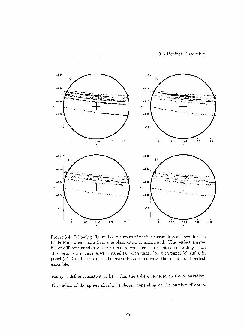
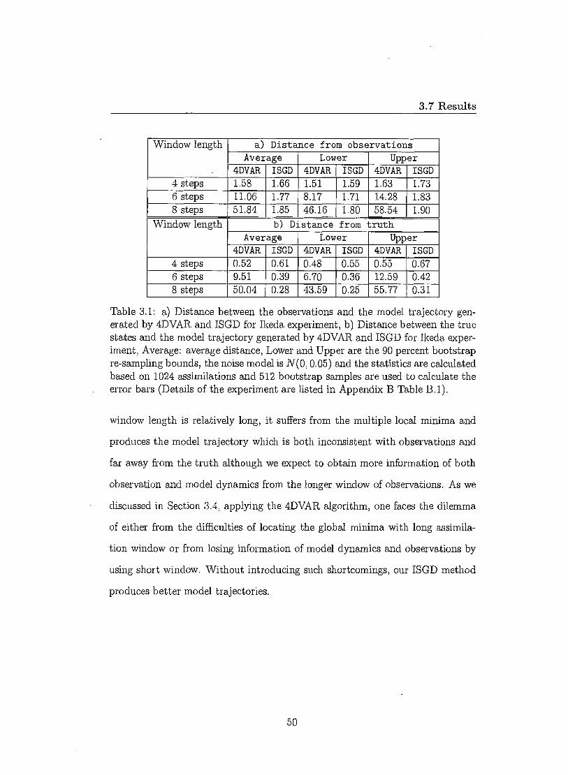
From Table 3.1 and 3.2, we can see that when the assimilation window is
short for both Ikeda and Lorenz96 experiments, both 4DVAR and ISGD tend to
generate model trajectories that are closer to the true states than to the obser-
vations 1 . This is expected as both methods can be treated as noise reduction
method. For ISGD method, the larger window length is considered, the better
model trajectories are produced. We expect the ensemble formed based on the
reference trajectory to produce better ensemble forecast when the reference tra-
jectory is closer to the true states of the system. For 4DVAR method, when the
'Although the trajectories is slightly father away from the observations, they are still con-sistent with the observational noise.
2 closer to the true states of the system
49
3.7 Results
Window length a) Distance from observations Average Lower Upper
4DVAR ISGD 4DVAR ISGD 4DVAR ISGD 4 steps 1.58 1.66 1.51 1.59 1.63 1.73 6 steps 11.06 1.77 8.17 1.71 14.28 1.83 8 steps 51.84 1.85 46.16 1.80 58.54 1.90
Window length b) Distance from truth Average Lower Upper
4DVAR ISGD 4DVAR ISGD 4DVAR ISGD 4 steps 0.52 0.61 0.48 0.55 0.55 0.67 6 steps 9.51 0.39 6.70 0.36 12.59 0.42 8 steps 50.04 0.28 43.59 0.25 55.77 0.31
Table 3.1: a) Distance between the observations and the model trajectory gen-erated by 4DVAR and ISGD for Ikeda experiment, b) Distance between the true states and the model trajectory generated by 4DVAR and ISGD for Ikeda exper-iment, Average: average distance, Lower and Upper are the 90 percent bootstrap re-sampling bounds, the noise model is N(0, 0.05) and the statistics are calculated based on 1024 assimilations and 512 bootstrap samples are used to calculate the error bars (Details of the experiment are listed in Appendix B Table B.1).
window length is relatively long, it suffers from the multiple local minima and
produces the model trajectory which is both inconsistent with observations and
far away from the truth although we expect to obtain more information of both
observation and model dynamics from the longer window of observations. As we
discussed in Section 3.4, applying the 4DVAR algorithm, one faces the dilemma
of either from the difficulties of locating the global minima with long assimila-
tion window or from losing information of model dynamics and observations by
using short window. Without introducing such shortcomings, our ISGD method
produces better model trajectories.
50
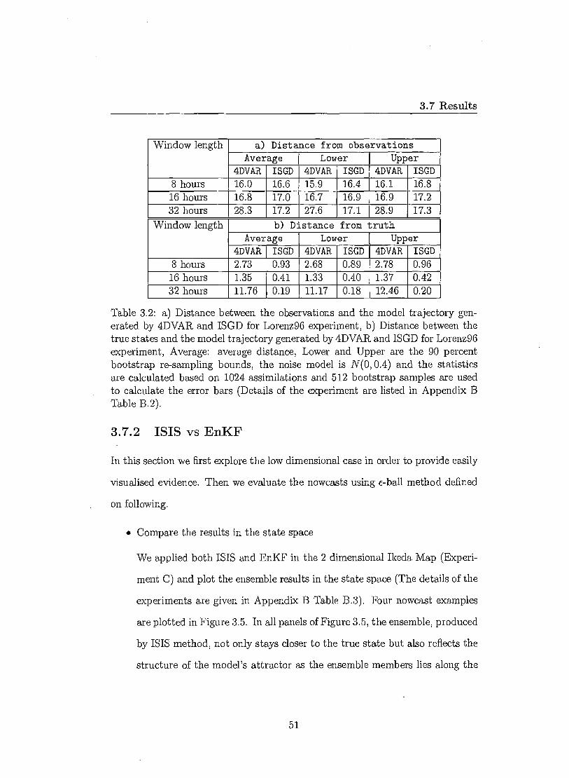
3.7 Results
Window length a) Distance from observations Average Lower Upper
4DVAR ISGD 4DVAR ISGD 4DVAR ISGD 8 hours 16.0 16.6 15.9 16.4 16.1 16.8 16 hours 16.8 17.0 16.7 16.9 16.9 17.2 32 hours 28.3 17.2 27.6 17.1 28.9 17.3
Window length b) Distance from truth Average Lower Upper
4DVAR ISGD 4DVAR ISGD 4DVAR ISGD 8 hours 2.73 0.93 2.68 0.89 2.78 0.96 16 hours 1.35 0.41 1.33 0.40 1.37 0.42 32 hours 11.76 0.19 11.17 0.18 12.46 0.20
Table 3.2: a) Distance between the observations and the model trajectory gen-erated by 4DVAR and ISGD for Lorenz96 experiment, b) Distance between the true states and the model trajectory generated by 4DVAR and ISGD for Lorenz96 experiment, Average: average distance, Lower and Upper are the 90 percent bootstrap re-sampling bounds, the noise model is N(0, 0.4) and the statistics are calculated based on 1024 assimilations and 512 bootstrap samples are used to calculate the error bars (Details of the experiment are listed in Appendix B Table B.2).
3.7.2 ISIS vs EnKF
In this section we first explore the low dimensional case in order to provide easily
visualised evidence. Then we evaluate the nowcasts using c-ball method defined
on following.
• Compare the results in the state space
We applied both ISIS and EnKF in the 2 dimensional Ikeda Map (Experi-
ment C) and plot the ensemble results in the state space (The details of the
experiments are given in Appendix B Table B.3). Four nowcast examples
are plotted in Figure 3.5. In all panels of Figure 3.5, the ensemble, produced
by ISIS method, not only stays closer to the true state but also reflects the
structure of the model's attractor as the ensemble members lies along the
51

3.7 Results
model attractor. The EnKF ensemble, however, has its own structure as
the ensemble members do not lie along the model attractor. In the top two
panels of Figure 3.5, the EnKF ensemble manage to cover the true state and
tends to stay close to the model's attractor. While in bottom two panels of
Figure 3.5, the ensemble members are systematically off the attractor and
tend to stay close to the observations and not covering the true state.
• Evaluate both methods via 6-ball
Here we introduce a simple new probabilistic evaluation method, which
evaluate the ensemble forecasts without transforming it into probability
distribution.
Given the verification corresponding to the forecast at time t, in this case
the verification is the true state at t = 0. One can draw a hyper-sphere
with radius E (hereafter 6-ball) around the verification. For any methods,
one can record the probability mass that is inside different size of 6-ball.
One can compare the result between two methods by simply counting the
proportion of times one method beats the other. If the methods tie, both
methods win. When the size of the 6-ball is very small, we expect neither of
the methods to be able to have ensemble members inside the 6-ball. When
the size of the 6-ball is big enough, we expect all the ensemble members
will fall inside the c-ball. In both cases, both methods wins. When the size
of the 6-ball is neither too large nor too small, we can investigate which
method produces ensemble forecasts assigns more probability mass around
the verification. The advantage of the 6-ball method is that it is simple
and easy to implement. Note the weakness of this method is that it is not
52
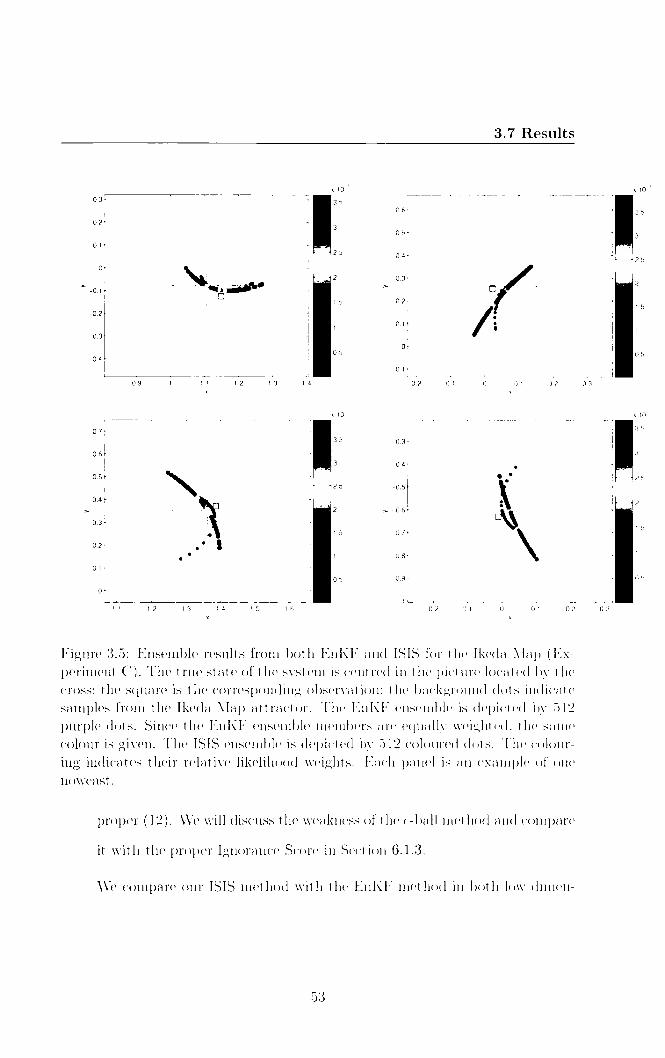
3.5 0.6
3 0.5
2.5 0.4
2
0.5
0.3
1.5 0.2
1 0.1
0
-0.1
x 10'
1 3.5 -03
3 -0.4
2.5 -0.5
2 ›.. -0.6
1.5 -0.7
1 -0.8
0.5 -0.9
x
-0.2
-0.2
-0. 1
-0.1
0
0
0.1
0.1
0.2
0.2
0.3
0.3
x10-3
3.5
3
2.5
2
1.5
1
0.5
x 10'
1.1 1.2 1.3 1.4 1.5 1.6
0.9
0.4
0.3
0.2
0.1
0
3.7 Results
x
Figure 3.5: Ensemble results from both EnKF and ISIS for the Ikeda Map (Ex-periment C). The true state of the system is centred in the picture located by the cross; the square is the corresponding observation; the background dots indicate samples from the Ikeda Map attractor. The EnKF ensemble is depicted by 512 purple dots. Since the EnKF ensemble members are equally weighted, the same colour is given. The ISIS ensemble is depicted by 512 coloured dots. The colour-ing indicates their relative likelihood weights. Each panel is an example of one nowcast.
proper (12). We will discuss the weakness of the E-ball method and compare
it with the proper Ignorance Score in Section 6.1.3.
We compare our ISIS method with the EnKF method in both low dimen-
53

3.7 Results
sional Ikeda Map (Experiment C) and higher dimensional Lorenz 96 model
I (Experiment D). The details of the experiments are given in Appendix B
Table l3.3 & B.I. In both cases we evaluate the nowcasting performance
using E-ball. Figure 3.6 shows the comparison between EnKF and ISIS.
From the figures, it appears that the ensemble generated by ISIS outper-
forms the one generated by EnKF for almost all different sizes of the epsilon
balls in both higher dimensional Lorenz96 and low dimensional Ikeda Map
experiments.
3.7.3 ISIS vs Dynamically consistent ensemble
In this section, we compare the nowcasting performance of ISIS ensemble with
that of the dynamically consistent ensemble (DCEn). For the purpose of simplic-
ity and efficiency, in the following experiments only uniform bounded noise model
is used to create the observations. Since finding the perfect ensemble members in
the high dimensional case is extremely cost, we will only compare the results in
the low dimensional Ikeda Map (Experiment E). Similar to the previous section,
we first compare both methods by looking at the ensemble results in the state
space and then we compare them by the c ball method. As we mentioned in
section 3.6, the more observations are considered, the better DCEn member can
be found. In Figure 3.7, 3.8, 3.9, 3.10, we compare the ISIS results (with fixed
window length, i.e. each window contains 12 observations) with the results pro-
duced by DCEn where different number of observations are considered. Details
'Note we expect both methods wins when the size of the 6-ball is very small or very large. In the Ikeda experiment, it happens when the size of the 6-ball less than 0.001 or larger than 1 although it is not seen in panel a) of Figure 3.6. And in the Lorenz96 experiment it happens when the size of the 6-ball larger than 6 although it is not seen in panel b) of Figure 3.6.
54
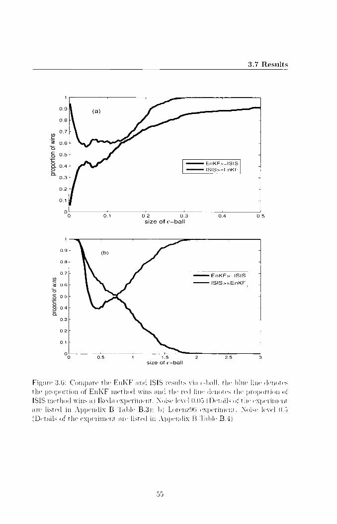
EnKF>=ISIS
ISIS>=EnKF
o o 0.4 0 5
0.9
0.8
0.7 CO
§ 0.6 0 S 0.5
*-E -) o.4
0_ 0.3
0.2
0.1
0.9
0.8
0.7 CI,
0.6
EnKF>=ISIS ISIS>=EnKF
oo 0.5 2 2.5 3
0
0 0.5
o_ 0.4 0
CD_ 0.3
0.2
0.1
3.7 Results
Figure 3.6: Compare the EnKF and ISIS results via &ball, the blue line denotes the proportion of EnKF method wins and the red line denotes the proportion of ISIS method wins a) Ikeda experiment, Noise level 0.05 (Details of the experiment are listed in Appendix B Table B.3); b) Lorenz96 experiment, Noise level 0.5 (Details of the experiment are listed in Appendix B Table B.4)
55
3.7 Results
of the experiment are given in Appendix B Table B.5. It appears that when the
DCEn is constructed by considering a small number of observations (e.g. 1 or 2),
the ISIS ensemble built on 12 observations outperforms the DCEn as shown in
Figure 3.7, 3.8. From the first four panels of Figure 3.7 and 3.8, we found that
some of the DCEn members lie on the same model's attractor as the true state
does, some are not while the ISIS ensemble seems to be lying on the right model's
attractor. And by evaluating the nowcast ensemble using e-ball method, we found
the ISIS ensemble assigns more probability mass around the true state than the
DCEn for almost all different sizes of E ball. This is due to the fact that lim-
ited dynamical information are contained in such short window of observations.
When more observations are considered the DCEn outperforms the ISIS ensem-
ble. Figure 3.9 shows that even using half window-size of the observations, the
DCEn outperforms the ISIS ensemble. The DCEn seems to be more concentrated
and closer to the true state than the ISIS ensemble and assign more probability
mass around the true state. Using the same length of the observations, with no
surprise the DCEn again wins.
As we discussed in Section 3.6, the DCEn is the optimal ensemble estimates
one may achieve. It is expected to outperform any other state estimation meth-
ods. Although our ISIS ensemble, with no doubt, underperforms the dynamically
consistent ensemble, it seems to have similar structure as the dynamically con-
sistent ensemble does. Note the ISGD algorithm is run for finite time, with more
ISGD iterations, we conjecture the ISIS ensemble will converges to the DCEn.
In practice, DCEn is computationally inapplicable while our IS methods can be
applied in both low dimensional and high dimensional systems (53).
56

„. 0
•
•
4tom T:
s
- 1.02
-1.04
- 1.08
-1.08
-1.1
-1.12
- 1,14
- 1.18
- 1.18
-1.2
- 0.66
-0.86
-0.7
-0.72
-0.74
-0.76
- 0.78
-0.8
-0.82
- 0.84
0.31 0.32 0.33 034 0.35 0.38 037 0.38 0.39 0.4 0.06 0.07 0.08 0.09 0.1 0.11 0.12 0.13 0.14 0.15
" • •
1.14 1.15 1.18 1.17 1.18 1.19 1.2 1.21 122 123 -003 -0.02 -0.01 0 0.01 0.02 0.03 0.04 0.05 0.06
0.32
0.3
028
0.26
024
0.22
02
0.18
0.18
0.14
1.88r1 ens wins IS ens wins
0.9
0.8
0.7
W
•
0.6
0.5
g- 0.4
0.3
0.2
0.1
0.05
- 096
-0.08
- 0.12
- 0.14
-0.18
1
-02
- 022
-024
•1
3.7 Results
Figure 3.7: Dynamically consistent ensemble built on 1 observation compared with ISIS ensemble built on 12 observations, the noise model is U(-0.025,0.025), each ensemble contains 64 ensemble members. The top four panels following Figure 3.5, plot the ensemble in the state space. The ISIS ensemble is depicted by green dots. The DCEn is depicted by purple dots. The bottom panel fol-lowing Figure 3.6 compare the DCEn and ISIS results via &ball. (Details of the experiment are listed in Appendix B Table B.5)
57
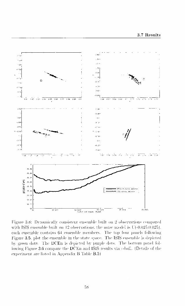
Per! ens wins IS ens wins
0.9
0.8
0.7
0.04 0.05 0.01
0.6
0.5
g- 0.4
0.3
0.2
0.1
0 0.02 0.03
size of eps-ball
3.7 Results
0
0.31 0.32 0.33 0.34 0.35 0.38 0.37 0.38 0.39 0.4
0.02
0
-0.02
-0.04
- 0.06
.• -0.08
-0.1
- 0.12
- 0.14
-0.16
1.06 1.07 1.06 1.09 1.1 1.11 1.12 1.13 1.14 1.15
•:•,.S: ❑
0.06 0.07 0.08 0.09 0.1 0.11 0.12 0.13 0,14 0.15
❑
t
0.27 0.28 0.29 0.3 0.310.32 0.33 034 0.35 0.36 X
-0.66
-0.68
-0.7
-0.72
-0.74
- 0.76
-0.78
-0.8
-0.82
-0.84
-0.06
- 008
-0.1
-0.12
-0.14
-0.16
- 0.18
-0.2
-022
-0.24
- 1.02
-1.04
- 1.06
- 1.08
-1.1
- 1.12
- 1.14
-1.18
- 1.18
-1.2
Figure 3.8: Dynamically consistent ensemble built on 2 observations compared with ISIS ensemble built on 12 observations, the noise model is U(-0.025,0.025), each ensemble contains 64 ensemble members. The top four panels following Figure 3.5, plot the ensemble in the state space. The ISIS ensemble is depicted by green dots. The DCEn is depicted by purple dots. The bottom panel fol-lowing Figure 3.6 compare the DCEn and ISIS results via c-ball. (Details of the experiment are listed in Appendix B Table B.5)
58
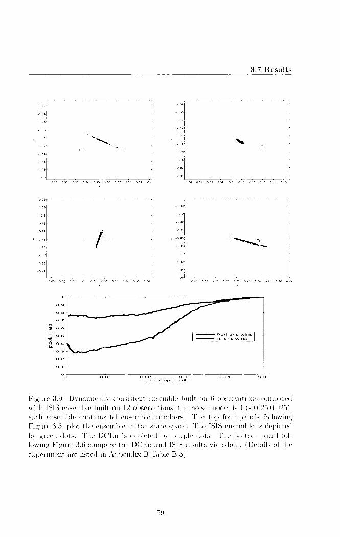
0
- 1.02
- 1.04
-1.08
-1.08
- 1.14
-1.16
-1.18
-1.2
-0.66
-0.68
- 0.7
- 0.72
-0.74
-0/6
- 0.78
- 0.8
- 0.82
-0.84
0.31 0.32 0.33 034 0.35 0.36 0.37 0.38 0.39 04 0.06 0.07 0.04 0.09 0.1 0.11 0.12 0.13 0.14 0.15
-0.03 -0.02 -0.01 0 0.01 0.02 0.03 004 0.05 006 0.68 0.69 0.7 0.71 0.72 0.73 0.74 0.75 0.76 0.77
-0.06
- 0.08
-0.1
-0.12
-0.14
-0.18
- 0.18
-0.2
-0.22
-0.24
-0.88
-0.9
- 022
-0.94
a. -0.96
- 0.98
-1
-1.02
- 104
1 06
Pert ens wins IS ens wins.
0.0
0.0
0.7
' 0.6
• 0 . 5
§- 0.4
0.3
0.2
0.1
0.05
3.7 Results
Figure 3.9: Dynamically consistent ensemble built on 6 observations compared with ISIS ensemble built on 12 observations, the noise model is U(-0.025,0.025), each ensemble contains 64 ensemble members. The top four panels following Figure 3.5, plot the ensemble in the state space. The ISIS ensemble is depicted by green dots. The DCEn is depicted by purple dots. The bottom panel fol-lowing Figure 3.6 compare the DCEn and ISIS results via e-ball. (Details of the experiment are listed in Appendix B Table B.5)
59

0
0.06 0.07 0.08 0.09 0.1 0.11 0.12 0.13 014 0.15
- 1.02
-1.04
106 • 0.68 0.69 0/ 0/1 0.72 0.73 0.74 0.75 0.79 0.77
0.05
-0.66
-OAS
-0.7
-0.72
-0.74
-0.76
-0.78
-0.8
-092
-0.64
43.88
-0.9
-0.92
-0.94
-096
-016 0
3.7 Results
Figure 3.10: Dynamically consistent ensemble built on 12 observations compared with ISIS ensemble built on 12 observations, the noise model is U(-0.025,0.025), each ensemble contains 64 ensemble members. The top four panels following Figure 3.5, plot the ensemble in the state space. The ISIS ensemble is depicted by green dots. The DCEn is depicted by purple dots. The bottom panel fol-lowing Figure 3.6 compare the DCEn and ISIS results via &ball. (Details of the experiment are listed in Appendix B Table B.5)
60
3.8 Conclusions
3.8 Conclusions
In this chapter, we considered the problem of estimating the current states of
the model in the perfect model scenario. Based on the Indistinguishable States
Theory, reviewed in Section 3.2, a new methodology is introduced to address the
nowcasting problem. Our methodology involves first applying the ISGD algorithm
to identify a reference trajectory which reflects the set of indistinguishable states
of the true state. The ISIS method is then introduced to form the ensemble by
selecting the model trajectories from the set of indistinguishable states of the
reference trajectory.
The well established 4DVAR method is reviewed and the difference between
4DVAR method and ISGD method is discussed. Applying both method to Ikeda
Map and Lorenz96 Model I, we demonstrate that the ISGD method produces
more consistent results than 4DVAR method. This result comes with no surprise
due to the fundamental shortcoming of the 4DVAR method, i.e. one faces the
dilemma of either from the difficulties of locating the global minima with long
assimilation window or from losing information of model dynamics and obser-
vations by using short window. The widely used sequential method EnKF is
reviewed and discussed. Comparisons between ISIS method and EnKF method
have been made in low dimensional Ikeda map and higher dimensional Lorenz96
model. By looking at the ensemble results in the state space, we find that the
structure of the ensemble obtained by ISIS method is more consistent with the
model dynamics than that of the ensemble produced by EnKF method. A new
simple evaluation method, &ball, is introduced to evaluate the nowcasting results
of both methods. We find that in both Ikeda Map and Lorenz96 model experi-
61
3.8 Conclusions
ments, our method systematically assigns more probability mass around the true
state than the EnKF method.
The optimal ensemble, dynamically consistent ensemble (perfect ensemble),
is described. Although the DCEn outperforms the ISIS ensemble, we found the
ensembles they produce have similar structure as both methods produce the en-
sembles that reflect the dynamical information of the model. In practice, DCEn
is computationally inapplicable while our IS methods can be applied in both low
dimensional and high dimensional systems (53).
62

Chapter 4
Parameter estimation
In this chapter we consider the problem of parameter estimation of deterministic
nonlinear models. The future evolution of the nonlinear dynamical models de-
pend strongly on the initial conditions and parameter specifications. As forecast
errors of nonlinear models will not be Gaussian distributed even if the observation
errors are drawn from Gaussian distribution, tradition methods like least squares
are not optimal. Methods have been developed to address the shortcomings of
traditional methods, for example estimating model parameters by incorporating
the global behaviour of the model into the selection criteria (64). Two new alter-
native approaches are introduced in this chapter within the perfect model scenario
(PMS) where the mathematical structure of the model equations are correct and
the noise model is known, but the true parameter values are unknown. The first
approach forms the cost function based on probabilistic forecasting, we call it
Forecast Based Estimates. The second approach focuses on the geometric prop-
erties of trajectories in short term while noting the global behaviour of the model
in the long term, we call this method Dynamical Coherent Estimates. Dynamical
63

4.1 Technical statement of the problem
Coherent Estimates is also applicable to the case that only partial observations
are available. We will first define the problem of parameter estimation in Sec-
tion 4.1. The traditional Least Squares estimates method is then described and
discussed in section 4.2. Forecast Based Estimates and Dynamical Coherent Es-
timates are presented in section 4.3 and section 4.4 respectively. Our approaches
are compared with Least Squares Estimates and the numerical results are shown
on several nonlinear models. Fundamental challenges remain in estimating model
parameters when the system is not a member of the model class. Discussions of
applying both methods to the case that the model structure is imperfect and
defining optimal parameter values are presented in section 4.5.
4.1 Technical statement of the problem .
Suppose the evolution of a system state xi E le is governed by finite dimensional
discrete deterministic nonlinear dynamics:
= , (4.1)
where the system's parameters are contained in the vector a E R1 . In the Per-
fect Model Scenario (see section 3.1), the model state space and system state
space are identical. F(x, a) of a model is known to match that of the system
exactly, i.e. F = F. Suppose the value for the vector of model parameters a is
unknown and must be estimated from observations s i of the state variables
Assuming additive measurement error m yields observations s i = xi + m, where
m is IID distributed. Without measurement error, l + 1 sequential measure-
64

4.2 Least Squares estimates
ments si , si+1 would, in general, be sufficient to identify the true param-
eter a (64). In the presence of observational noise, the true state of the system
3-4 can not be determined precisely even infinite observations are provided and
the parameter values are known exactly (48). As we will see, this also makes the
problem of parameter estimation much harder.
In this chapter we focus on addressing the problem of parameter estimation
in the perfect model scenario. Our aim is to extract the information from a finite
series of observations given the exact noise model and the functional form of the
dynamic model to determine the model parameter values.
We never identify the true model parameter precisely of course; rather we
introduce two methods for extracting significant information on parameter values,
one via evaluating the probabilistic forecast performance that they produce; the
other via the trajectories they admit. And how to report the parameter estimates
based on our methods are discussed.
4.2 Least Squares estimates
The famous least squares method (8; 27; 56) estimates the parameter by testing
the error in the forecast initialised at observations. The one-step least squares(LS)
estimate gives the value of parameter which minimises the least squares cost
function.
N -1
CLS (a)
rri , (4.2) i=1
65

4.2 Least Squares estimates
where ern = s i+i — F(s i , a), the one-step prediction error. The LS cost function
can be derived from Maximum Likelihood Estimate(MLE) (17). Assume the
observational noise and the forecast error, i.e. s i+1 — F(s i , a), are IID Gaussian
distributed with mean 0 and standard deviation a. Given the observations s t , t
1, the likelihood function of parameter a is then given by
1 , L(a) = (27r0_2)N/2 expl — st+i — (4.3)
By minimising the log likelihood function, i.e. log(L(a)), the Least Squares cost
function is then derived. IVIcsharry and Smith (64) proved that even with an
infinite amount of data the optimal least squares solution is biased when it applied
to the 1-D Logistic Map. Figure 4.1 plots the least square estimates against
different noise level 1 for both Logistic map and Ikeda map. Figure 4.2 plots
the Least Squares cost function in the parameter space for both Moore-Spiegel
System and Henon Map experiments, given the noise level fixed. We can see
from both figures that Least Squares Estimates systematically rejects the correct
parameter value and from Figure 4.1, the higher the noise level is, the more bias
in the estimate (20). The LSE method fails simply because the assumption of
Independent Normal Distributed (IND) forecast errors does not hold even if the
noise is IND.
1 The different noise levels in the plots are defined by the ratio between the standard devi-ation of the observation noise and the standard deviation of the signal
66
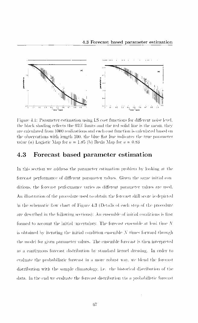
15.
0. 09
(b)
07-
01 02 03 04 05 06 02 08 0
anousia9ignffil
4.3 Forecast based parameter estimation
Figure 4.1: Parameter estimation using LS cost functions for different noise level, the black shading reflects the 95% limits and the red solid line is the mean, they are calculated from 1000 realizations and each cost function is calculated based on the observations with length 100, the blue flat line indicates the true parameter value (a) Logistic Map for a = 1.85 (b) Ikeda Map for u = 0.83
4.3 Forecast based parameter estimation
In this section we address the parameter estimation problem by looking at the
forecast performance of different parameter values. Given the same initial con-
ditions, the forecast performance varies as different parameter values are used.
An illustration of the procedure used to obtain the forecast skill score is depicted
in the schematic flow chart of Figure 4.3 (Details of each step of the procedure
are described in the following sections): An ensemble of initial conditions is first
formed to account the initial uncertainty. The forecast ensemble at lead time N
is obtained by iterating the initial condition ensemble N times forward through
the model for given parameter values. The ensemble forecast is then interpreted
as a continuous forecast distribution by standard kernel dressing. In order to
evaluate the probabilistic forecast in a more robust way, we blend the forecast
distribution with the sample climatology, i.e. the historical distribution of the
data. In the end we evaluate the forecast distribution via a probabilistic forecast
67
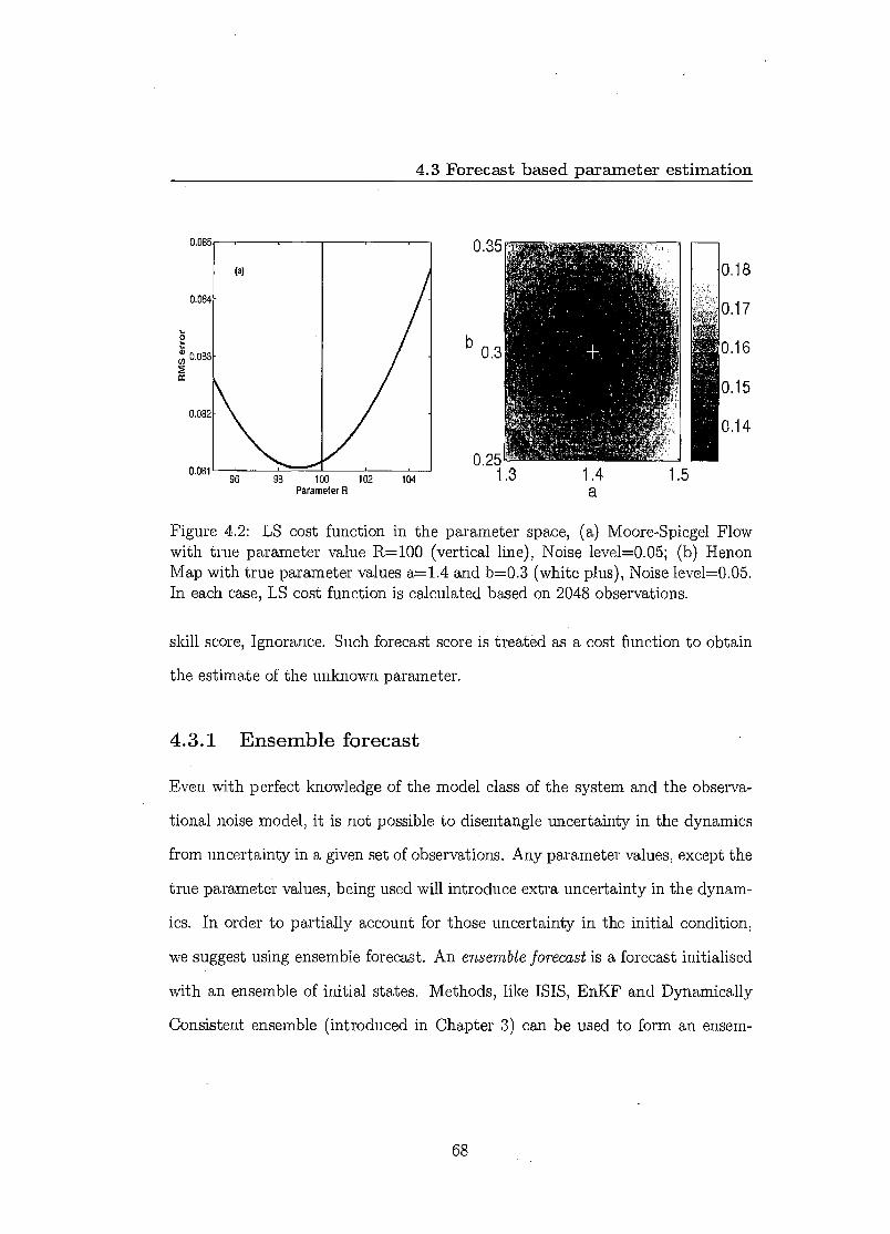
104 1.3 1.4 a
1.5
0.085
0.084
2 tn°3 0.083
cc
0.082
b 0.3
0.25
0.18
0.17
0.16
0.15
0.14
0.35
4.3 Forecast based parameter estimation
Figure 4.2: LS cost function in the parameter space, (a) Moore-Spiegel Flow with true parameter value R=100 (vertical line), Noise level=0.05; (b) Henon Map with true parameter values a=1.4 and b=0.3 (white plus), Noise level=0.05. In each case, LS cost function is calculated based on 2048 observations.
skill score, Ignorance. Such forecast score is treated as a cost function to obtain
the estimate of the unknown parameter.
4.3.1 Ensemble forecast
Even with perfect knowledge of the model class of the system and the observa-
tional noise model, it is not possible to disentangle uncertainty in the dynamics
from uncertainty in a given set of observations. Any parameter values, except the
true parameter values, being used will introduce extra uncertainty in the dynam-
ics. In order to partially account for those uncertainty in the initial condition,
we suggest using ensemble forecast. An ensemble forecast is a forecast initialised
with an ensemble of initial states. Methods, like ISIS, EnKF and Dynamically
Consistent ensemble (introduced in Chapter 3) can be used to form an ensem-
68

4.3 Forecast based parameter estimation
An initial condition ensemble
Mo del Ffr, a)
Forecast ensemble at lead time N
Kernel dressing
Model forecast distribution Blending
with
Final forecast distribution Evaluate
the forecast
Cost function for parameter a
Figure 4.3: Schematic flowchart of obtaining forecast based cost function for parameter estimation
ble of initial states. Here we adopt another simple method, called Inverse Noise
(Defined in the following paragraph), to form the initial condition ensemble.
69
4.3 Forecast based parameter estimation
Given a model of the observational noise, one can add random draws from
the inverse of the observational noise model to the observation to define ensemble
members. As each ensemble member is an independent draw from the inverse
observational noise distribution, each ensemble member is equally weighted. This
Inverse Noise method is an easy way to form the ensemble although the initial
states are not guaranteed to 1 be consistent with the long term model dynamics
i.e. the ensemble members are not on the attracting manifold of the model (if
there is one). For purposes of illustration and simplicity, most results shown in
section 4.3.4 are obtained by using Inverse Noise instead of other sophisticated
state estimation methods (Discussed in chapter 3) to form the ensemble.
4.3.2 Ensemble interpretation
Ensemble members are often transformed into a distribution function which is
easier to express the information contains in the ensemble members and it can
be evaluated by forecast skill scores. Continuous forecast distributions can be
produced from an ensemble by kernel dressing the ensemble forecast. In this
section we give a brief introduction to standard kernel dressing which will be
used to explain the problem in this section (see (13; 75) for more details). We
define an Nens member ensemble at time t to be X t ..., xr] and treat all
ensemble members as exchangeable. In other words, the ensemble interpretation
methods do not depend on the ordering of the ensemble members (13).
A standard kernel dressing approach is to transform the ensemble members
into a probability density function:
'guaranteed not to, in the case of dispersive dynamics.
70

4.3 Forecast based parameter estimation
(4.4)
where
1 1 K(() = TIT exP(- 2 5 2 ), (4.5)
where y is a random variable corresponding to the density function p and KO is
the kernel density function, for standard kernel dressing we use standard Gaussian
density to be the kernel density function.
In this case a standard kernel dressed ensemble is a sum of Gaussian kernels.
Each ensemble member is replaced by a Gaussian kernel centred at x i . The
width of each kernel, called the kernel width, is given by the standard deviation
of the Gaussian kernel. The kernel width as one of the parameters of ensemble
interpretation can be determined by optimising the expected performance, for
example the ignorance score introduced in the next section, based on a training
set of ensemble and its verification pairs.
We are aware that the variance of the standard kernel dressed ensemble is
always larger than the variance of the raw ensemble, no matter how the kernel
width is actually determined (93). When the ensemble is over dispersive, or in
other words, the ensemble members are further away from each other than from
the verification, the standard kernel dressing may even under-performs the Gaus-
sian fit (93). In practice, ensembles tend to be under dispersive. Many advanced
and complicated dressing methods exist, for example Brocker (13) introduced an
71

4.3 Forecast based parameter estimation
improved kernel dressing, called "affine kernel dressing" that is more flexible and
robust kernel dressing method. In this chapter we use standard kernel dressing
to produce the results as it is straightforward to understand and implement.
For any finite ensemble, there remains the chance that the verification lies out-
side the range of the ensemble. Even if the verification is selected from the same
distribution as the ensemble itself, the probability of this happening is — 2 Nens •
Given the nonlinearity of the model, these points may be very far from the en-
semble, and appear as "outliers" or "bad busts". Those outliers will affect the
kernel width significantly by making them wider in order to make the forecast
distributions cover them which therefore degrades the performance of probabil-
ity forecast where the outliers do not appear. To overcome such problems, we
combine the forecast distribution with the sample climatology. As we mentioned
in Section 2.3, the sample climatology 1 is the distribution of the historical data
which can also be treated as an estimate of observed invariant measure of the sys-
tem. The probability density function of climatology can be approximated from
the historical data simply by kernel dressing the historical data. In this thesis we
use standard kernel dressing to approximate the density function of climatology.
The probabilistic forecast can be improved on average by blending model forecast
distribution, which is obtained from the dressed ensemble, with the climatology.
By blending with the climatology, defines the forecast distribution to be:
PO = aPm• + ( 1 — cf)Pc(')
(4.6)
where pm is the density function generated by dressing the ensemble and p c is the
1 We will often drop the word "sample" afterwards
72

4.3 Forecast based parameter estimation
estimate of climatological density, the subscript m denotes the model and c the
climatology. a E [0, 1], called blending parameter, denotes the weight assign to
the model forecast distribution.
Note that comparing forecast performance of different models may provide
a misleading comparison without blending climatology. As it might be the case
that, without blending climatology Model A outperforms Model B while with
blending climatology this is not the case.
4.3.3 Scoring probabilistic forecasts
A probability forecast describes our expectation of how likely an event is on a
particular occasion. One may wish to ask whether a probability forecast is right
or wrong. Unlike point forecasts, however, single probability forecasts have no
such clear sense of "right" and "wrong". One can only measure how good the
probabilistic forecasts are by looking at a large set of forecasts. Conventional
diagnostics for evaluating deterministic forecasts, measures such as "root-mean-
square error", are not useful with probabilistic forecasts (37).
A probabilistic forecast skill score is a function S(p(y), Y), where Y is the ver-
ification and p(y) is a probability density. Following Good (1950), Roulston. and
Smith (2001) introduced a measure of the quality of the forecasting scheme, which
is called Ignorance. Ignorance is a logarithmic scoring rule that can be calculated
for real forecasts and realizations. It is equivalent to the expected returns that
would be obtained by placing bets proportional to the forecast probabilities (75).
And Ignorance is the only proper local score for continuous variables (12; 75).
The Ignorance Score is given by:
73

4.3 Forecast based parameter estimation
S(P(Y), = —log(p(Y))
(4.7)
The difference between the Ignorance scores of two forecast schemes, reflects the
expected wealth doubling time under a Kelly Betting. 1 We employ the ignorance
score to evaluate the probabilistic forecast in this thesis. In practice, we have to
go to empirical since we have limited data. Given N forecast-verification pairs
(Pt, Yt, t = 1,...,N) (forecast-verification pair are a forecast and what actually
happened, for example a forecast probability distribution of the temperature in
London Heathrow and the temperature actually observed), the empirical average
Ignorance skill score is given by:
SEmp(P(Y), Y) — log(P(Y)) (4.8)
This empirical average Ignorance skill score is used as a cost function to estimate
the parameter values of the model in the results shown in next section. In practice,
we can get an idea how accurate of uncertainty in our empirical ignorance by
bootstrapping.
'In a Kelly betting contest (57), one bets all of one's wealth on every outcome in proportion to the forecast probability of that outcome. More precisely, a fraction wi of ones wealth, where co, is the forecast probability of event .E2, occurring, should be wagered on the ith outcome.
74
4.3 Forecast based parameter estimation
4.3.4 Results
In order to demonstrate the effectiveness of our method, parameter estimation
by forecast performance is applied to both one and two dimensional systems and
results are compared with Least Squares estimates. Figure 4.4a shows the cost
function, i.e. Ignorance score, based on probabilistic forecast at lead time 4 for
the logistic map, where initial condition ensemble is formed by Inverse Noise.
Results of different noise levels are plotted separately. When the noise level is
relative large for example 1/8, the information contained in the forecast is unable
to tell the difference between the parameter values. When the noise level is small
enough, estimates obtained by looking at the Ignorance score of the probabilistic
forecast well identifies the parameter values as the minimum ignorance occurs
at the vertical line that marks the true parameter value. Figure 4.4b plots the
Ignorance cost function of forecast at lead time 4 in the parameter space for
the Henon map, same observations are used as Figure 4.2b. The low ignorance
region (black) captures the true parameter values. Comparing with LS estimates
(Figure 4.2b), using Ignorance as a cost function produces more consistent results.
The forecast based parameter estimate results shown in Figure 4.4a and Fig-
ure 4.4b are based on the probabilistic forecast at lead time 4. The particular
lead time was chosen because the cost functions at such lead time produce more
consistent results. Figure 4.5 shows the forecast based parameter estimates for
different lead times. Note there is a bias at short lead time. Also note that
although estimates at longer lead time provides more consistent results, the cost
function becomes less sharp as lead time gets larger. Examining graphs of several
lead times (Figure 4.5), it was found that those of lead time 4 were consistent for
75
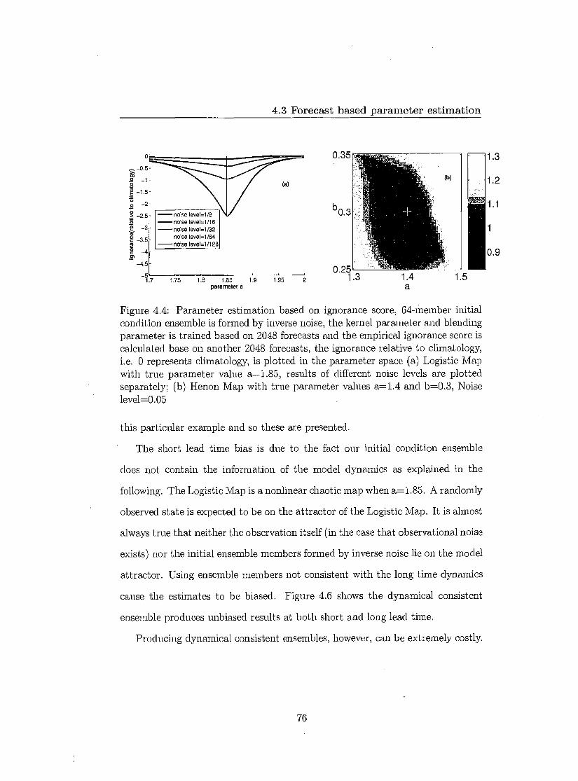
0.35
b0.3
0.25 1.3 1.4
a 1.5
(a)
0
▪ —0.5 C, {,2 —1 a E —1.5 .
noise level=1/8 — noise level=1/16 — noise level=1/32
noise level=1/64 — noise level."' /128
2 —4
—4.5
o —2
>
•
—2.5
ia! —3
`t'' —3.5
4.3 Forecast based parameter estimation
Figure 4.4: Parameter estimation based on ignorance score, 64-member initial condition ensemble is formed by inverse noise, the kernel parameter and blending parameter is trained based on 2048 forecasts and the empirical ignorance score is calculated base on another 2048 forecasts, the ignorance relative to climatology, i.e. 0 represents climatology, is plotted in the parameter space (a) Logistic Map with true parameter value a=1.85, results of different noise levels are plotted separately; (b) Henon Map with true parameter values a=1.4 and b=0.3, Noise level=0.05
this particular example and so these are presented.
The short lead time bias is due to the fact our initial condition ensemble
does not contain the information of the model dynamics as explained in the
following. The Logistic Map is a nonlinear chaotic map when a=1.85. A randomly
observed state is expected to be on the attractor of the Logistic Map. It is almost
always true that neither the observation itself (in the case that observational noise
exists) nor the initial ensemble members formed by inverse noise lie on the model
attractor. Using ensemble members not consistent with the long time dynamics
cause the estimates to be biased. Figure 4.6 shows the dynamical consistent
ensemble produces unbiased results at both short and long lead time.
Producing dynamical consistent ensembles, however, can be extremely costly.
76
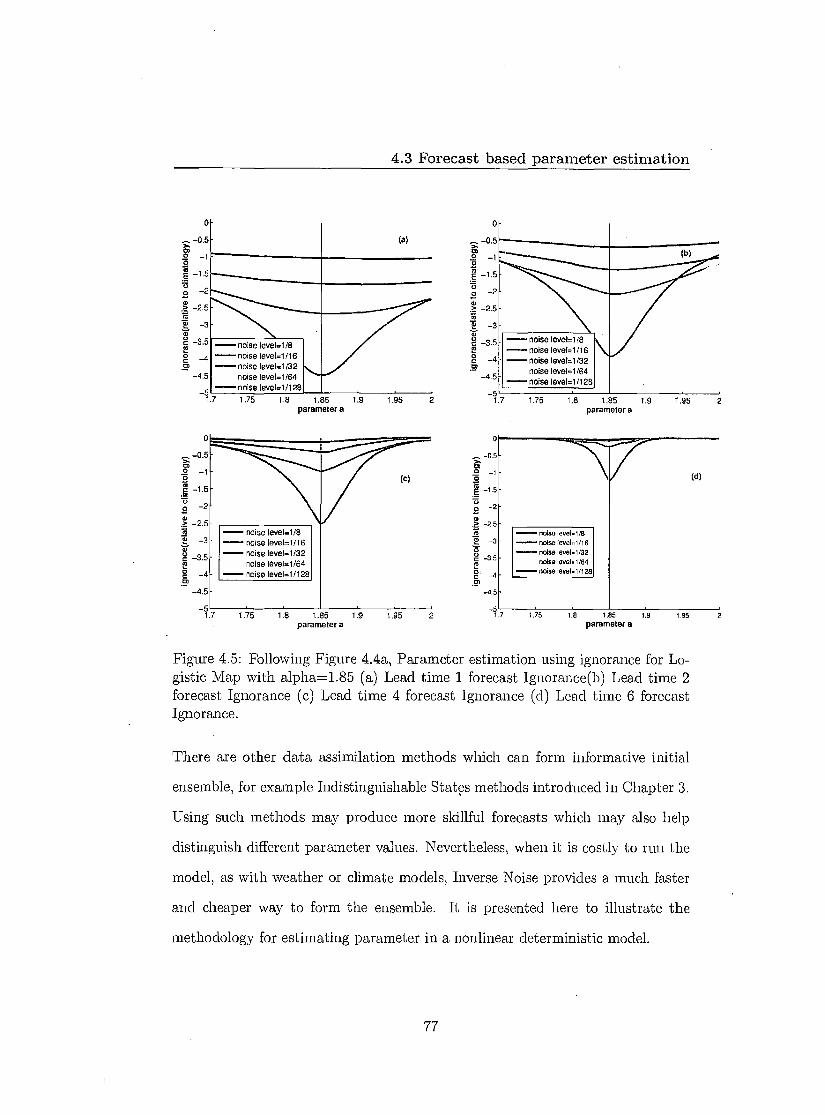
1.9 1.95
rs _3 -
a, - noise level=1 /8 - noise level=1 /16 - noise level=1 /32
noise level=.1 /64 - noise level=1 /128 -5
1.7 1.75 1.8 1.85 parameter a
(a)
0 -
-0.5 rn
- noise level=1 /8 noise level=1 /16
- noise lever=1 /32 noise lever=1 /64 noise level=1/128
-5 17 1.75 1.8 1.85 1.9 1.95 2
parameter a
(b)
2 -3
2 -3.5
g -4
-4.5
0-
-2.5
c° -3.5
c -4
- -4.5
4.3 Forecast based parameter estimation
0
-0.5 S.; er) :1 -1
E -1.5
o -2 a)
-2.5 a -3
2 -3.5
S -4
-4.5
-5
0
-0.5 a.
2 -1 (C) 2
-t.5
o -2 to o• -2.5
-3
2 -3.5 2 c -4 rn
-4.5
(d)
noise level=1/8 nolso leve1.1/B - noise level=1/16 --- noise revel-1/1B
- noise level-1/32 noise leve1.1/64
- noise leve1=1 /32 noise level=1 /64 noise leve1.1 /128 - noise level-1/128
17
1.75 1.8 1.85 1.9 1.95
7 1.75 1.8 1.85 1.9 1.95 parameter a parameter a
Figure 4.5: Following Figure 4.4a, Parameter estimation using ignorance for Lo-gistic Map with alpha=1.85 (a) Lead time 1 forecast Ignorance(b) Lead time 2 forecast Ignorance (c) Lead time 4 forecast Ignorance (d) Lead time 6 forecast Ignorance.
There are other data assimilation methods which can form informative initial
ensemble, for example Indistinguishable States methods introduced in Chapter 3.
Using such methods may produce more skillful forecasts which may also help
distinguish different parameter values. Nevertheless, when it is costly to run the
model, as with weather or climate models, Inverse Noise provides a much faster
and cheaper way to form the ensemble. It is presented here to illustrate the
methodology for estimating parameter in a nonlinear deterministic model.
77
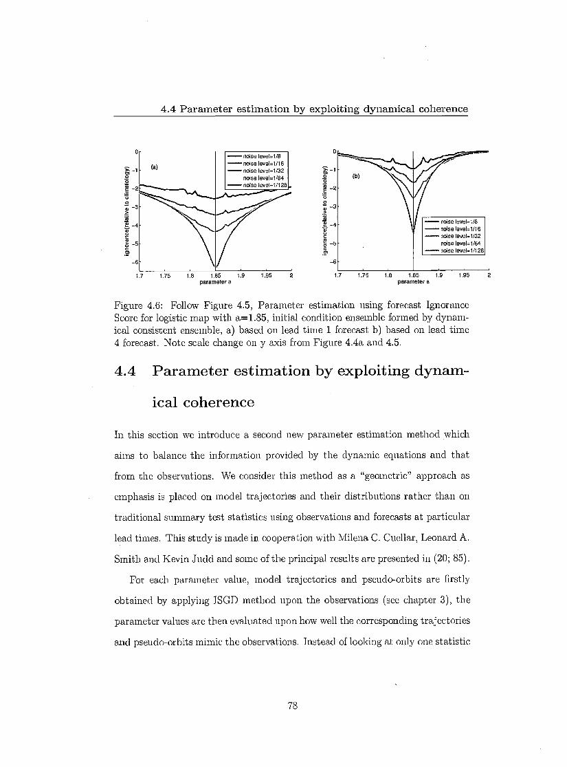
-- noise level=1/8 - noise level=1116 - noise level=1/32
noise level=1/64 - noise level=1/128
- noise level=1/8 - noise level=1/16 - noise level=1/32
noise level=1/64 - noise level=1/128
4.4 Parameter estimation by exploiting dynamical coherence
Figure 4.6: Follow Figure 4.5, Parameter estimation using forecast Ignorance Score for logistic map with a=1.85, initial condition ensemble formed by dynam-ical consistent ensemble, a) based on lead time 1 forecast b) based on lead time 4 forecast. Note scale change on y axis from Figure 4.4a and 4.5.
4.4 Parameter estimation by exploiting dynam-
ical coherence
In this section we introduce a second new parameter estimation method which
aims to balance the information provided by the dynamic equations and that
from the observations. We consider this method as a "geometric" approach as
emphasis is placed on model trajectories and their distributions rather than on
traditional summary test statistics using observations and forecasts at particular
lead times. This study is made in cooperation with Milena C. Cuellar, Leonard A.
Smith and Kevin Judd and some of the principal results are presented in (20; 85).
For each parameter value, model trajectories and pseudo-orbits are firstly
obtained by applying ISGD method upon the observations (see chapter 3), the
parameter values are then evaluated upon how well the corresponding trajectories
and pseudo-orbits mimic the observations. Instead of looking at only one statistic
78
4.4 Parameter estimation by exploiting dynamical coherence
or measurement, we measure i) the consistency between model trajectories and
observations by shadowing time; ii) how well model pseudo-orbits approximate
relevant trajectories by the mismatch error and iii) the consistency between the
implied noise distribution (corresponding to the model pseudo-orbits) and the
noise model.
Within the perfect model scenario, there exists a parameter set (for the dy-
namic model and the noise model) which admits the true trajectory which did,
in fact, generate the observed data. Our method is aiming to identify such set by
exploiting dynamical coherence. Outside PMS the preferred cost function will un-
doubtedly depend upon the application; parameters which admit long shadowing
times seem a good choice for forecast models.
4.4.1 Shadowing time
Although superficially similar, the question of whether a model shadows a set
of observations is a fundamentally different notion from the traditional ques-
tion of whether or not one mathematical system can shadow the trajectories of
another (26; 31; 33; 58; 77; 83). Traditional shadowing (77) involves two well-
defined mathematical systems. Our ultimate interest here is between a set of
observations and a proposed model. Given a segment of observations s o , ..., sN ,
we are interested whether there exists a model trajectory (for a given parameter
value) x0 , ..., xN that the residuals defined by the trajectory and the observa-
tions, i.e. si — x i , i = 0, ..., N, are consistent with the observational noise model.
For an observation s o at initial time t = 0, the corresponding shadowing time
;0 is the largest K such that, there is some model state x 0 , the time series
79

4.4 Parameter estimation by exploiting dynamical coherence
ri = si — F( ) (xo , a), i = 0, ...,K is consistent with the noise model.
In order to calculate the shadowing time, one must evaluate the consistency
between a series of residuals and the noise model in some way. For uniform
bounded noise this is straightforward: A series of residuals r K is consistent
with the noise model when every residual is inside the bound. For unbounded
noise model, for example Gaussian distribution, there are a variety of approaches
to test whether a series points are drawn from the given distribution, for example
Chi-Square test and Kolmogorov-Smirnov test. In our methodology we adopt
a simple method based on threshold exceedance to do the test. Given that the
noise model is unbounded, any observation is conceivable; we look for relevant (9)
shadows within a certain probability bound. For purposes of illustration and sim-
plicity, we use the scalar to illustrate the procedure. We test the null hypothesis
that the set of residuals (r i , i = 0, 1, 2, K) is consistent in distribution with in-
dependent draw from the noise distribution. The shadowing time is then defined
to be the largest K that the null hypothesis is not rejected at the 99.9% signifi-
cant level. To accept the null hypothesis, we require both that the 90% isopleth
of the residual distribution falls below the 99 th percentile of the distributions of
90% isopleths given K draws from a Gaussian distribution, and that the median
of the residual distribution falls below the corresponding 90 th percentile for the
median of the noise model (Note: The thresholds will vary with the size of the
data set and the noise model). Together this implies that the chance rejection
rate is 0.001, which will yield good results as long as the shadowing times we test
are below 100 (as they are in the results presented in section 4.4.3).
For a given observation time, we are most interested in the trajectory which
shadows the longest and is consistent with the observation made at that time.
80

4.4 Parameter estimation by exploiting dynamical coherence
In practice we consider only a finite set of candidate trajectory segments. Call
these candidates 4, j = 1, ..., iv, where .AT, is the number of candidates (the
subscript c denotes candidate). For each observation define the shadowing time
Ts = maxx Ts (xic ) where the maximum is taken over all candidates x e values tested.
Instead of random sampling around the observations, we derive more useful can-
didates from relative pseudo-orbits. Following section 3.3, given a sequence of
observations, a pseudo-orbit of the model can be derived by ISGD method. Of
course the quality of the pseudo-orbit strongly depends on the parameter values,
which also links the quality of the parameter value to the candidates used to
calculate shadowing time. Points along a pseudo-orbit can be used as candidate
initial conditions of trajectory segments. In the results presented below in sec-
tion 4.4.3, only three candidates per observation were tested: the corresponding
point on the pseudo-orbit, the image of the previous point on the pseudo-orbit,
and the point midway between these two.
As for each observation s t , it has its corresponding shadowing time, for a
segment of observations we have a distribution of shadowing time. Our idea
is using the shadowing time distribution to estimate the parameter values by
identifying the interest area in the parameter space. The parameter estimation
method introduced in section 4.3 quantifies how well the dynamics of the model
mimic the observations at a fixed lead time. The shadowing time distribution is
a different flavour of quality statistic, quantifying the time scales over which the
dynamics of the system reflect those of the data.
81

4.4 Parameter estimation by exploiting dynamical coherence
4.4.2 Further insight of Pseudo-orbits
As the model pseudo-orbits obtained by the ISGD method strongly depend on
the parameter values, the dynamical information contained in the pseudo-orbits
can help highlight areas where the estimates can be considered as candidates for
"good" estimations in the parameter space (20). In this section we extract such
information by looking at the remaining mismatch error and the implied noise of
the model pseudo-orbits.
As the ISGD algorithm, introduced in Section 3.3, is iterated for a finite num-
ber of steps, the minimum of the mismatch cost function, i.e 0, is not reached
and therefore a model pseudo-orbit is obtained instead of model trajectory. The
remaining mismatch error after a fix number of iterations of the ISGD algo-
rithm indicates how well the model pseudo-orbit converges to a model trajectory.
For each parameter value, the speed of convergence also indicates how easily a
corresponding model trajectory can be found. Therefore the magnitude of the re-
maining mismatch as a quality of the model pseudo-orbit can be used to identify
the interesting areas in the parameter space.
As the model pseudo-orbit can be treated as the estimate of the true states
in the model space, the quality of the pseudo-orbit can also be evaluated by the
consistency of the corresponding implied noise (defined in section 3.3) distribu-
tion with the noise model. With finite ISGD iterations, it generally appears to be
the case that the final pseudo-orbit obtained corresponding to the true parame-
ter values has an implied noise level no more than the true noise level, inasmuch
as we initialise the ISGD algorithm with the observations and aim to explicitly
minimise the mismatch cost function. The pseudo-orbit corresponding to the
82
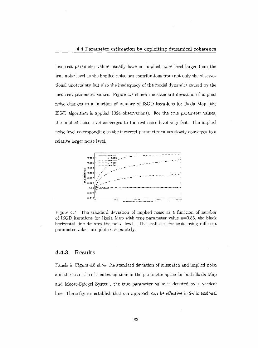
4.4 Parameter estimation by exploiting dynamical coherence
incorrect parameter values usually have an implied noise level larger than the
true noise level as the implied noise has contributions from not only the observa-
tional uncertainty but also the inadequacy of the model dynamics caused by the
incorrect parameter values. Figure 4.7 shows the standard deviation of implied
noise changes as a function of number of ISGD iterations for Ikeda Map (the
ISGD algorithm is applied 1024 observations). For the true parameter values,
the implied noise level converges to the real noise level very fast. The implied
noise level corresponding to the incorrect parameter values slowly converges to a
relative larger noise level.
u 0.83 u=0.825 0.026
0.025
3.1 0.024
-o 0.023
g 0.022
73 0.021
0.019
0.0180 500
1000 1500 number of ISGD itoralion6
Figure 4.7: The standard deviation of implied noise as a function of number of ISGD iterations for Ikeda Map with true parameter value u=0.83, the black horizontal line denotes the noise level. The statistics for tests using different parameter values are plotted separately.
4.4.3 Results
Panels in Figure 4.8 show the standard deviation of mismatch and implied noise
and the isopleths of shadowing time in the parameter space for both Ikeda Map
and Moore-Spiegel System, the true parameter value is denoted by a vertical
line. These figures establish that our approach can be effective in 2-dimensional
2000.
83
4.4 Parameter estimation by exploiting dynamical -coherence
chaotic maps, 3-dimensional chaotic flows. Before discussing these individually,
note that in each case the vicinity of the true parameter value is clearly indicated.
The distribution of shadowing time for several isopleths are shown for both
the Ikeda system (panel a) and the Moore-Spiegel third order ODE (panel d)
in Figure 4.8. The median and 90% contour provide good parameter estimates,
while the 99% contour suffers from sampling effects. The choice of isopleth is
not critical, although sampling noise will, of course, become an issue for extreme
values of the distribution. Thresholds will vary with the size of the data set
and the noise model; a simple bootstrap re-sampling approach can identify how
high an isopleth can be robustly estimated. In addition to shadowing time, the
vicinity of the true parameter value also provide small mismatch error (panel
(b) and (e)) and their implied noise level is consistent with the true noise model
(panel (c) and (f)). Note in Figure 4.8e, the true parameter does not provide the
smallest mismatch error. As we mentioned in Section 4.4.2, the mismatch error
is obtained by fixed number of iterations for each parameter value. It indicates
how easily a corresponding model trajectory can be found. It is possible that
for some parameter values other than the truth, it is easier for the pseudo-orbit
to converge to a model trajectory under Gradient Descent. However the model
trajectory may not consistent with the observations which can be testified by
looking at the shadowing time distribution and implied noise distribution. We
suggest looking at the distribution of shadowing time, the mismatch error and
the distribution of implied noise together instead of looking at only one of them.
Comparing with results shown in Figure 4.1(b) and Figure 4.2(a), our method
outperforms least squares estimate approach significantly.
Figure 4.9 shows the results for simultaneous estimation of the two parameter
84

3.5
3
E 2.5
2 S 1.5
0.5
4.4 Parameter estimation by exploiting dynamical coherence
1.053 MOM-Spiegel Sysied
0525
1.052
0515
1.051
0505
O.
O. 95 96 97 98 99 100 101 102 103 104 105
Figure 4.8: Parameter estimations for Ikeda Map with u=0.83 and noise level=0.02; Moore-Spiegel System with R=100 and noise level=0.05, the results are calculated base on 1024 observations, (a) and (d) The median (solid), 90% (dashed) and 99% (dash-dot) shadowing isopleths; (b) and (e) standard deviation of the mismatch; (c) and (1) standard deviation of the implied noise, the horizon-tal line denotes the real noise model. The vertical line represents the location of the unknown true parameter.
85

4.4 Parameter estimation by exploiting dynamical coherence
values in the Henon Map, where the standard deviation of the mismatch and the
implied noise level are shown in addition to the median of the shadowing time
distribution and a cost-function based on the invariant measure (after (64)). The
fine structure ("tongues") in panel (c) is due to sensitivity to the parameters,
nevertheless its minima are in the relevant regions. Contrasting panels (c) and
(d) of figure 4.9 reveals that shadowing times provide information complimentary
to that obtained by estimating the invariant measure (the CML of (64)). The
shadowing time distribution provide complimentary information quantifying the
time scales on which the model dynamics reflects the observed behaviour. Com-
paring the results with Figure 4.2b, our method provides more consistent results.
Statistics of the shadowing time distribution provide and unambiguous indication
of the range of relevant parameter values.
4.4.4 Application in partial observational case
Here we consider the case of parameter estimation in higher dimensional systems
where the state vector is not completely observed, i.e. some components of the
system are unobserved. In such case, i) we firstly estimate the unobserved com-
ponents by simply random draw from the climatology of observed components.
ii) We then initialise the ISGD algorithm with the observed components and
the estimates of the unobserved components. A pseudo-orbit is obtained after
a small number of ISGD iterations. iii) We then update the estimates of the
unobserved components with the relative components of the pseudo-orbit. Re-
peating ii) and iii) several times in order to obtain an "good" estimates of the
unobserved components. In the end we run a large number ISGD iterations to ob-
86

0.2 1.5
0.35
b 0.3
0.5
0
4.4 Parameter estimation by exploiting dynamical coherence
Figure 4.9: Information from a pseudo-orbit determined via gradient descent applied to a 1024 observations of the flexion map with a noise level of 0.05. (a) standard deviation of the mismatch, (b) the implied noise level, (c) a cost function based on the model's invariant measure (after Fig.4(b) of ref (1 , (d) median of shadowing time distribution.
87

Parameter F
0 9 9.2 9.4 9.6 9.8 10 10.2 10.4 10.6 10.8 11
Pamela, F
(9)
4
3.5
e 25
2
1.5
0.6
E
1 2
0.5
as
2.5
1.5
■ • .....
o 9 9.2 a4 9.6 9.8 10 10.2 10.4 10.6 10.8 11
o 9 9.2 9.4 9.6 9.8 10 10.2 10.4 10.6 10.8 11
3
4
(C)
0.5
4
as
3
2.5
2
(d)
4.4 Parameter estimation by exploiting dynamical coherence
taro the pseudo-orbit which is used to calculate the shadowing time distribution.
In such cases the shadowing-time is determined without placing any constraints
whatsoever on the value taken by the unobserved component(s).
Figure 4.10: Shadowing time isopleths as in Figure 4.8 for 8-D Lorenz96 with parameter F=10 given only partial observations, a) the 8th component of the state vector is not observed; b) none of the 2nd, 5th or 8th variables are observed only the other five components; c) only 2nd, 5th or 8th variables are observed; d) all the components of the state vector are observed. In this experiment the noise level is 0.2.
Figure 4.10 shows the result of the application in the 8-D Lorenz96 system.
Panel (d) shows the isopleths for the 8 dimension Lorenz96 system with states
fulled observed. It appears that our method provides good parameter estimates
88

4.5 Outside PMS
in the higher dimensional model case. In panel (a) seven of the eight components
of the state vector are observed, in panel (b) 5 of the eight components are
observed and in panel (c) only 3 components are observed. In all cases, the
correct parameter values are well indicated although the length of shadowing
time decreases as less components are observed.
4.5 Outside PMS
Large forecast-verification archives and lower observational noise level contain
more information and thus yield better parameter estimates when the model
structure is perfect. When the model class does not admit on empirically adequate
model, the notation of a "true" parameter value is lost. It is important to note
that even if the true parameter values are unknown, they are well defined within
PMS; the question of defining optimal parameter values when the model structure
is imperfect is more complex.
The experiment of forming probabilistic forecast to estimate parameter values
is also useful at identifying "best" parameter in an imperfect model if a notation
of best is defined as best forecast performance at certain lead time.
The geometric approach using shadowing time and additional statistics of
the pseudo-orbit is also useful to identify parameter values which can mimic
the dynamics, quantify the time scales on which they can shadow and extract
information for improving the model class itself. Even in systems as unwieldily
as multi-million-dimensional operational climate models, variations in parameters
over the relevant range of uncertainties yield demonstrably nonlinear effects (87)
in the most basic summary statistics (i.e. climate sensitivity). The ISGD methods
89
4.6 Conclusions
have been used on models of this level of complication (51). Outside PMS there
may be no single optimal parameters, of course, but even in this case shadowing
times have the advantage of providing information on likely lead times at which
a forecast will have utility. Timescales on which the dynamics of the model are
consistent with the noise model and the observations can be of use in setting the
window of observations to be used, and the effectiveness of, variational approaches
to data assimilation (51).
4.6 Conclusions
In this chapter, we considered the problem of estimating the parameter values
of the model in the perfect model scenario. Traditional linear method, Least
Squares estimates, is unable to produce consistent results due to the fact that the
assumption of Independent Normal Distributed(IND) forecast does not hold when
the model is nonlinear. To address the shortcomings of traditional methods, two
new alternative approaches, Forecast Based estimates and Dynamical Coherent
estimates, are introduced in this chapter.
For Forecast Based estimates, we estimate the parameter values based upon
the probabilistic skill of the model as a function of parameter values. This
straightforward procedure has been shown to yield good parameter estimation
in several chaotic maps. Forecast based estimation using Inverse Noise ensembles
is straightforward to implement and relatively computationally inexpensive. We
have shown that it can suffer biases when the ensemble is not distributed consis-
tently with respect to the models long term dynamics (invariant measure). We
have also shown that, for addition computational investment to sample a perfect
90

4.6 Conclusions
ensemble this bias can be removed.
Dynamical Coherent estimates is presented which focuses on the geometry
of trajectories of the model rather than the forecast performance at a given lead
time. We estimate the parameter values based upon i) the ability of model trajec-
tories to shadow by looking the shadowing time distribution; ii) how well model
pseudo-orbits approximate relevant trajectories by measuring the mismatch error
of the pseudo-orbits; iii) the consistency of the distribution of implied-noise with
the noise model. ISGD method is applied to obtain candidates with longer shad-
owing time and the model pseudo-orbit. The technique is illustrated for both
flows and maps, applied in 1, 2, 3 and 18 dimensional dynamical systems, and
shown to be effective in a case of incomplete observation where some components
of the state are not observed at all.
Outside PMS, although the optimal estimates of the parameter is not well
defined, we suggest our approaches may still be able to produce robust results.
91

Chapter 5
Nowcasting Outside PMS
When forecasting real systems, for example the Earth's atmosphere as in weather
forecasting, there is no reason to believe that a perfect model exists. Generally
the model class from which the particular model equations are drawn does not
contain a process that is able to generated the data. In this case we are in the
Imperfect Model Scenario (IPMS), and it is crucial to distinguish the model(s)
from the system which generated the data.
In the Perfect Model Scenario, given the infinite CPU power, one may be able
to form a perfect ensemble (80), whose members are drawn from the same distri-
bution as the system state. In the IPMS, however, such a perfect ensemble does
not exist. Any ensemble data assimilation scheme is expected to result with an
probabilistically unreliable state estimation. This chapter is concerned with how
to forecast the current state using ensemble methods given the observations and
imperfect model. In the IPMS, model state space and the system state are usually
different. In this chapter we are aiming to estimate the initial states of the model
for the purpose of forecasting. In this case not only the observational uncertainty
92

but also the model inadequacy need to be considered when an ensemble of initial
conditions is constructed.
In the Imperfect Model Scenario, methods assuming the model is perfect
may be inapplicable and in any event they would seem unlikely to produce the
optimal results. It is almost certain that no trajectory of the model is consistent
with an infinite series of observations (50), thus there is no consistent way to
estimate the model states using trajectories. There are pseudo-orbits, however,
that are consistent with observations and these can be used to estimate the model
state (50). In this chapter we applying the same ISGD algorithm as discussed in
previous chapter, but with a new stopping criteria to find relevant pseudo-orbits
outside PMS.
The Imperfect Model Scenario is defined and two system-model pairs are set
up in Section 5.1. Section 5.2 discusses various Indistinguishable States methods
of finding a pseudo-orbit and demonstrates that our new methodology, i.e. apply-
ing the ISGD method with certain stopping criteria, can find better pseudo-orbits.
Other method, such as Weakly Constraint 4DVAR, is discussed and compared
with our method in Section 5.3. Results of comparing the pseudo-orbit produced
by ISGD method and WC4DVAR method are presented in Section 5.5.1. This is
the first time IS methods and the WC4DVAR method are compared in the IMPS.
Methods of forming the ensemble based on the pseudo-orbits are introduced and
discussed in Section 5.4 and the results of nowcasting is presented in Section 5.5.2.
93
5.1 Imperfect Model Scenario
5.1 Imperfect Model Scenario
Outside pure mathematics, the perfect model scenario is a fiction. Arguably,
there is no perfect model for any physical dynamical system (50).
In the Imperfect Model Scenario (IPMS), we define a nonlinear system with
state space Wh, the evolution operator of the system is F, i.e. 5ct+i = E(Rt)
where ict E Rth is the state of the system. An observation s t of the system
state "Xt at time t is defined by s t = h(Rt ) m where st E 0, m represents
the observational noise, in this thesis we assume Tit are IID distributed; h(.) is
the observation operator, which projects the system state into the observation
space 0. For simplicity, we take h(.) to be the identity. Consider a model, which
represents the system approximately, with the form x t+1 = F(xt ), where xt E M,
M is the model state space. Assume the system state x can also be projected into
the model state space by a projection operator g(•), i.e. x = g(51). In general,
we don't know the property of this projection operator, we don't know even if
5"c exists. We are just going to assume that it maps the states of the system
into somehow relevant states in the model. For the purposes of illustration and
simplicity, unless otherwise stated, we assume g(.) is one-to-one identity. A better
understanding of g(•) is beyond the scope of this thesis but it is an important
point for additional work. Our aim is to estimate the current state of the model
xo given the previous and current observations s t , t = —n + 1, ..., 0.
In the imperfect model scenario, the model is inadequate. Following Smith and
Judd (2004), two types of model inadequacy are investigated. One is structurally
incorrect model inadequacy, the other is ignored subspace model inadequacy. For
each type of model inadequacy, an example is given, where both the true system
94

5.1 Imperfect Model Scenario
and a class of models are listed. These model-system pairs are used to construct
and compare the state estimation methods in the following sections.
• Structurally inadequacy
This type of model inadequacy appears where the system dynamics are not
known in detail and its mathematical structure is different from that of
the model. Here we use the Ikeda Map and truncated Ikeda model as an
example of this case (50). The Ikeda system is a two dimensional map (see
section 2.4), P : W. The mathematical functions of the system are:
xTh+1 = + u(x„, cos — y, sin 0) (5.1)
Yn+i = u(xr, sin 0 + cos 0), (5.2)
where 0 = 13 — a/(1 + xn2 + yTh2 ) and the parameter values used are a =
6, 3 = 0.4, -y = 1, u = 0.83. The imperfect model F is obtained by using
the truncated polynomial to replace the trigonometric function in F, i.e.
cos 0 = cos(w + 7r) + w3 /6 — 2/120 (5.3)
sin 0 = sin(w + 7r) w2/2 w4/24 (5.4)
where the change of variable to w was suggested by Judd and Smith (2004)
since 0 has the approximate range —1 to —5.5, and -7V is conveniently near
the middle of this range. In this case, the model state and the system state
share the same state space.
95
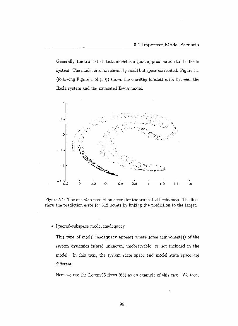
5.1 Imperfect Model Scenario
Generally, the truncated Ikeda model is a good approximation to the Ikeda
system. The model error is relevantly small but space correlated. Figure 5.1
(following Figure 1 of (51))) shows the one-step forecast error between the
Ikeda system and the truncated Ikeda model.
1
0.5
0
-0.5
-1
-1.5 -0 2 0 0.2 0.4 0.6 0.8 1
1.2 1.4
1.6
Figure 5.1: The one-step prediction errors for the truncated Ikeda map. The lines show the prediction error for 512 points by linking the prediction to the target.
• Ignored-subspace model inadequacy
This type of model inadequacy appears where some component(s) of the
system dynamics is(are) unknown, unobservable, or not included in the
model. In this case, the system state space and model state space are
different.
Here we use the Lorenz96 flows (63) as an example of this case. We treat
96
h dxi x c dt =
xi_ixi+i — xi F — —b J-1
dyj ,i hue = Yi+2,i) cYjo: 'x •
dt b
(5.5)
(5.6)
5.1 Imperfect Model Scenario
the Lorenz96 model II as the system that generates the data (details of
Lorenz96 models can be found in section 2.4). The mathematical functions
of the system are
for i = 1, n. The system used in our experiments containing n = 18
variables x 1 , ..., is with cyclic boundary conditions (where xn±i = x1 ).
Like the large scale variables x i , the small-scale variables have the cyclic
boundary conditions as well(that is ym+i,i = yi, i+i ) (in our experiments
m = 5).
The Lorenz96 model I is treated as the imperfect model (details of Lorenz96
models can be found in section 2.4). From the mathematical function
dxi dt = —xi_2xi_1 + x i_ ixi+i — x i + F (5.7)
one can see that the small dynamical variables y in the system equation ( 5.5
& 5.6) are not included in the Lorenz96 model I. The magnitude of error
made by the imperfect model depends on the coupling parameter /ix ,hy and
in our experiments we set both fi x and by to be 1. In this system and model
pair setting, the model state space and the system state space are different.
97

5.2 IS methods in IPMS
5.2 IS methods in IPMS
5.2.1 Assuming the model is perfect when it is not
What will happen if one ignores the model inadequacy and assumes that the
model is perfect. Here we investigate whether this would degrade state estimation
of the nonlinear system. And if so, how do the results from the perfect model
scenario, as shown in chapter 3, change when applied to imperfect models?
In the Perfect Model Scenario, there are a set of indistinguishable states H(i . )
that can not be distinguished from the system state 53 (48). In IPMS, however, it
is not necessary that IHI(i.) contains states other than itself. Even for the state FC
itself, the projection i of the system trajectory defined by x into the model space
is not a trajectory of the model, which means no state of model is consistent
with the observations. This situation can arise even when the model trajectory
remains in proximity to (the observed part of) the system trajectory (50).
If we ignore the model inadequacy and apply the ISGD algorithm to find a
model trajectory, we will find that the minimisation converges very slowly to
zero when the window length is very long, which implies no model trajectory is
"close" to the observations. In the results shown in 5.2.5, the results of state
estimation by applying ISGD algorithm to minimise the mismatch degrade after
certain iterations of gradient descent.
5.2.2 Model error
In this chapter we will consider the point-wise model error to be Sc- ri+ i — F(in ). It
might be reasonable to assume the observational noise is IID distributed. But it
lassume the projection is one-to-one identity
98

5.2 IS methods in IPMS
is almost certain that the model error of a nonlinear model is not IID distributed.
For example in Figure 5.1, the model error between the truncated Ikeda model
and Ikeda system is spatially correlated; there are regions where the model error
is small and regions where it is not. Understanding the distribution of the model
error aids in model development. If systematic model errors are identified, one
can improve the model by correcting some of the errors. In this chapter, we are
less interested in improving the model than in how to obtain states of the model
for initial conditions which, for insistence, serve the purpose of forecast given the
imperfect model. Therefore, we assume that the model we use to approximate
the system is the best model one can achieve and the model errors have been
reduced to the minimum given the available information. In the later section, we
will discuss how the information about the model error can also help to improve
the quality of estimates of future states.
In the IPMS, to estimate the current state of the model, one need to account
the uncertainty from both observational noise and model inadequacy. Without
the observational noise, the model error can be derived from the observations
directly. In the presence of observational noise, compounding of model error
and observational noise prevent us identifying either of them precisely. Such
unsolvable problem also causes the state estimation more or less biased in the
IPMS.
5.2.3 Pseudo-orbit
Since no state of the model has a trajectory consistent with an infinite sequence
of observations of the system in the IPMS, any model trajectory must eventu-
99
5.2 IS methods in IPMS
ally be unable to maintain consistency between the observations and the model
dynamics. There are pseudo-orbits, however, that are consistent with observa-
tions and these can be used to provide better estimates of the projection of the
system state. Pseudo-orbits (50) are sequences of states of the model x t that
at each step differ from trajectories of the model, that is, x t+1 F(xt )• We
define the imperfection error of the pseudo-orbit x t to be co t = xt+i — F(xt)•
Note the imperfection error does not necessarily correspond to the model error,
however the projection of a system trajectory 1 in the model state space forms
a pseudo-orbit of the model where the imperfection error is exactly the model
error in the model state space. Recall that in the PMS, there are a set of in-
distinguishable states Eff(x) of the system state x. Each indistinguishable state
defines a system trajectory that consistent with both the observations and the
system dynamics. In the IPMS, the system trajectories are pseudo-orbits of the
model in the model space and these "true pseudo-orbits" are consistent with the
observations and the model dynamics and most important the imperfection er-
ror reflects the model error exactly. Unfortunately, such desirable pseudo-orbits
cannot be found in the Imperfect Model Scenario, because of the confounding
between observational noise and model error. One can, however, find relevant
(useful) pseudo-orbits of the model that are consistent with observational noise
and the imperfection error of those pseudo-orbits can be treated as estimates
of the model error or at least provide some information about the model error.
Methods, adopted based on ISGD method, of finding relevant pseudo-orbits are
introduced and discussed in the next two sections.
'assume the system states are one-to-one identically projected onto the model space
100

5.2 IS methods in IPMS
5.2.4 Adjusted ISGD method in IPMS
Judd and Smith (2004) introduced a method of finding relevant pseudo-orbits by
adjusting the ISGD method to include the model imperfection. A brief description
of this method is given here in order to introduce and compare with a new method
introduced in the next section.
Similar to the ISGD method introduced in section 3.3, Following Judd and
Smith (2004), Gradient Descent algorithm is applied to minimise the adjusted
mismatch error by including the model imperfection error term. For a finite
sequence of observations, St , t = —N +1, ..., —1, 0, we define the adjust mismatch
error for a sequence of pseudo-orbit zt to be
et = zt+i — wt-F1 — F(zi) (5.8)
where cot is the imperfection error.
Define the implied noise, 5 to be the difference between the pseudo-orbit and
the observations, i.e.
St = st — zt . (5.9)
Hence fore, the mismatch equation 5.8 can be written as
et =1 st+i cot+1 F(st — (50 • (5.10)
101
5.2 IS methods in IPMS
Consider cost function CM((5, w), where
0
CM(6,w) = et et, (5.11)
t=-N
is defined in order to find relevant pseudo-orbit by GD algorithm.
Following Judd and Smith (2004), one can find a pseudo-orbit from the se-
quence of observations by applying Gradient Descent to minimise the cost func-
tion CM(o, w). It is necessarily that CM(6, w) attains a minimum of zero. To
solve the minimisation by gradient descent, one need to solve the differential
equations
aL — — ab- aw (5.12)
to compute the asymptotic values of ((5, w) by initialising the cost function with
both 8 and w equal to 0. The resulting values of S and w defines a certain
pseudo-orbit.
Ignoring the model inadequacy, one may attempt to minimise CM(o, 0), which
equals to applying the ISGD method (see Section 3.3.2) to look for model trajec-
tory assuming that the model is perfect. Although the cost function CM(5, 0)
always has the minimum of zero regardless the model is perfect or not, the model
trajectory obtained when CM(6, 0) reaches 0, is expected to be far away from
the true states and be inconsistent with the observations as long as N is large
enough.
102

5.2 IS methods in IPMS
Recall that the relevant pseudo-orbits we are looking for are those consis-
tent with the observations and their corresponding imperfection errors contains
information about the model error or somehow reflects the model error. The
implied noise 6 provides an estimate of the observational noise and the imper-
fection error w provides an estimate of the model error. In order to improve the
method and find better pseudo-orbits, we measure the quality of the pseudo-orbit
by looking at the RMS distance between pseudo-orbit and the projection of the
true trajectory of the system and testing the statistical consistency both between
the implied noise and the observation noise and between the imperfection error
and the model error. We are aware that when the system is nonlinear, linear
measurement like RMS has systematic bias (64) (see Chapter 4). The distance
between the pseudo-orbit and the true states may not reflect forecast skill in the
Imperfect Model Scenario. We only use this measurement as a diagnostic tool to
help explain how to construct a better method to locate relevant pseudo-orbit.
We investigate the quality of the pseudo-orbits generated by minimising the
cost function CM(5, 0) and CM(S, w) in both Ikeda and Lorenz96 system and
model pairs experiments.
Cost function No. of GD runs CM(O, •) std of (5t std of cot RMS distance C./14- (6, 0) 4096 0.025 0.051 0 0.0154 CM(S, co) 128 0.0002 0.037 0.02 0.012
Table 5.1: Statistics of the pseudo-orbits obtained by minimising the cost func-tion CM(6, 0) and C114- (6, w) for the experiment of Ikeda system-model pair. Minimisations are applied upon 4096 observations, the noise level is 0.05 and the sample standard deviation of the model error is 0.018.
From Table 5.1 and 5.2 one can see that firstly in both experiments, it is
much more difficult to minimise CM(S, 0) than CM(S, w) and the cost function
103

5.2 IS methods in IPMS
Cost function No. of GD runs CM(5,-) std of 5t std of wt RMS distance CM(S, 0) 4096 0.11 1.69 0 1.38 CM(6, w) 128 0.0006 0.63 0.46 0.52
Table 5.2: Statistics of the pseudo-orbits obtained by minimising the cost function CM(c5, 0) and CM(S,co) for the experiment of Lorenz96 system and model pair. The length of the sequence of observations is 102.4 time unit and the sampling rate is 0.025 time unit. The noise level is 1 and the sample standard deviation of the model error is 0.25.
CM(o, 0) does not appear to converge to zero. Secondly for both methods the
standard deviations of the implied noise and the imperfection error are very dif-
ferent from that of the observational noise and the model error (We are aware
that neither the model error nor the imperfection error is IID, there are infor-
mation of them beyond the second moment of their distribution. For simplicity
we use the standard deviation, as a diagnostic tool, to test consistency between
imperfection error and model error). The pseudo-orbit generated by minimising
CM(S, 0) stays too far away from the observations as the standard deviation of
implied noise is much larger than that of the observational noise, which indicates
that the pseudo-orbit obtained by minimising CM(S, 0) is not consistent with
observations. While the pseudo-orbit generated by CM(5, w) seems to stay too
close to the observations according to the standard deviation of implied noise.
The standard deviation of the imperfection error is larger than that of the model
error between the system and the model which indicates that the model error
is over-estimated by the imperfection error. From the RMS distance between
pseudo-orbit and true states in table 5.1 & 5.2, minimising CM(o, w) produces
pseudo-orbit closer to the truth. But apparently this method doesn't tackle the
problem of confounding between observational error and model error very well
as neither the implied noise is a good estimate of observational noise nor the
104

5.2 IS methods in IPMS
imperfection error is a good estimate of model error which may indicate that the
estimates of the model states are highly biased.
5.2.5 ISGD with stopping criteria
The GD method introduced by Judd and Smith (2004) is unable to produce a
desirable estimation of the projection of the system state as the implied noise
and imperfection error of the relevant pseudo-orbit are not consistent with the
observational noise and model error. Confounding between observational noise
and model error makes it impossible to produce pseudo-orbits whose implied
noise and imperfection error are consistent with observational noise and model
error respectively. We found that applying the ISGD method with proper stop-
ping criteria can, however, reduce such inconsistency and obtain less bias state
estimation results.
As we mentioned in the previous section, applying the ISGD method is equiv-
alent to minimise CM(6, 0) cost function, i.e. the mismatch cost function defined
in Section 3.12 and Equation 5.11 are the same. Examples shown in previous
section demonstrate that the minimisation does not converge to zero easily and
the pseudo-orbit produced eventually is not consistent with the observations and
stays farther away from the true pseudo-orbit than even the observations. When
the C./V/(6, 0) is greater than zero after finite iterations of GD, the mismatch error
e t is actually the imperfection error. In other words, minimising the CM(S, 0) is
actually minimising the imperfection error. If the imperfection error goes to zero,
the pseudo-orbit becomes a model trajectory. Since we treat the imperfection
error as the estimate of the model error which is known to exist when the model
105

5.2 IS methods in IPMS
is imperfect. Our purpose is not minimising the imperfection error but produc-
ing better or more consistent estimate of the model error. Figure 5.2 shows the
statistics of pseudo-orbit changes as a function of the number of iterations of
Gradient Descent minimising mismatch cost function CM(S, 0) in both higher
dimensional Lorenz96 system-model pair experiment and low dimensional Ikeda
system-model pair experiment (Details of the experiments are list in Appendix B
Table B.6.
Figure 5.2 shows that as the Gradient Descent minimisation iterates further
and further, the standard deviation of implied noise is getting larger and larger
which indicates that the pseudo-orbit is moving farther away from the observa-
tions. By comparing the standard deviation of implied noise with that of the real
noise model, we found that at the beginning of the minimisation, the observa-
tional noise is underestimated by the implied noise since the pseudo-orbit stays
too close to the observations. This makes sense because the minimisation algo-
rithm is initialised at the observations. As the minimisation proceeds, the implied
noise becomes more consistent with the observational noise and the pseudo-orbit
gets closer to the true pseudo-orbit. After a certain number of iterations, how-
ever, the implied noise tends to overestimated of the observational noise and the
distance between the pseudo-orbit and the projection of true system trajectory
gets larger. This is due to the model inadequacy. The minimisation makes the
imperfection error smaller. When the imperfection error of the pseudo-orbit be-
comes smaller than the actual model error, the implied noise has to compensate
for the imperfection error to account for the uncertainty caused by the model in-
adequacy which makes implied noise too large and the pseudo-orbit inconsistent
with the observations.
106

0.015
o 0.01
3 0.005
la)
4
100 202 300 400
500
600 number 01 iterations
(b)
e
-6.5
-7
-7.5
-8
100 150 200 250 300 350 400 number ol Iterations
0.2
018
0.16
0.14
0.12
2 0.1
0.08
1 006 S
0.04
0.02
-8.50
0.03
600
50 100 150 200 250 nurnboi Mile.lions
D.35
0.3.
0.4
300
350 400
5.2 IS methods in IPMS
Figure 5.2: Statistics of the pseudo-orbit as a function of the number of Gra-dient Descent iterations for both higher dimension Lorenz96 system-model pair experiment (left) and low dimension Ikeda system-model pair experiment (right). (a) is the standard deviation of the implied noise (the flat line is the standard deviation of the noise model); (b) is standard deviation of the model imperfection error (the flat line is the sample standard deviation of the model error); (c) is the RMS distance between pseudo-orbit and the true pseudo-orbit.
107

5.2 IS methods in IPMS
Since the model error is neither IID nor Gaussian distributed, how well the
imperfection error mimics the model error should not be judged only by the
statistics of the second moment. Figure 5.1 shows that the model error is spatially
correlated. As an estimation the model error, we expect the imperfection error has
similar spatial correlations as the model error. Figure 5.3 plots the imperfection
error in the state space with different GD iterations for the Ikeda Map. To
make comparison easier, Figure 5.1 is re-ploted in the fourth panel. The pictures
show that at the beginning of the minimisation, the imperfection error is larger
than the model error in most places. The pattern of spatial correlation can only
be seen around (0.5, —1.3), which suggests the imperfection error is not a good
estimate of the model error. This is because at the beginning of the minimisation,
the imperfection error contains both the observational error and model error.
Similarly after too many iterations, the imperfection error is forced to be small
and lose the spatial correlation it should have. One can see very little spatial.
correlation of imperfection error in the third panel. With a intermediate number
of iterations 1 , however, the imperfection error seems better estimate the model
error, the pattern in the second panel and fourth panel are very similar.
It might be asked whether the imperfection error estimates the model error
precisely? Unfortunately, it does not. Confounding between model error and
observational noise prevents us identifying either of them precisely (30). We
also found that how well the model error can be estimated strongly depends on
the signal magnitude between observational noise and model error. Figure 5.4
plots the imperfection error in the state space with intermediate GD iterations at
1 The number of iterations set up based on the statistics of imperfection error, generally we match the standard deviation of the imperfection error with that of the model error
108

1 1.2 1.4 1.6
0.5
0
-0.5
-1
5.2 IS methods in IPMS
1-
0.5 0.5 11,
.■11
0 f
0
':?ft .„2 .
-0.5 -0.5
-1
-1.5 '
0 "
0.2 0.4 '
0.6 '
0.8 1 1.2 1.4 1.6 -1.5
-0 2 -0.2
Figure 5.3: Imperfection error during the Gradient Descent runs for Ikeda Map case is plotted in the state space. (a) after 10 GD iterations, (b) after 100 GD iterations, (c) after 400 GD iterations (d) the real model error in the state space for comparison.
another two different noise levels. When the observational noise is much smaller
than the model error, the model error can be well estimated by the imperfection
error. When the observational noise is much bigger than the model error, the
imperfection error looks very close to random.
109
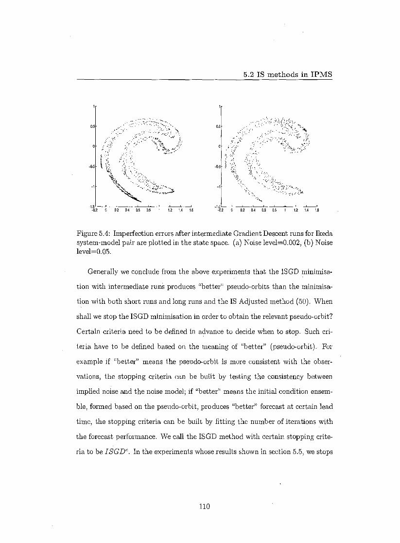
0.5
0
2 -1.5
-0 0 02 0.4 0.6 0.8 1.2 1.4 1.6
0.5
0
-0.5
5.2 IS methods in IPMS
Figure 5.4: Imperfection errors after intermediate Gradient Descent runs for Ikeda system-model pair are plotted in the state space. (a) Noise level=0.002, (b) Noise level=0.05.
Generally we conclude from the above experiments that the ISGD minimisa-
tion with intermediate runs produces "better" pseudo-orbits than the minimisa-
tion with both short runs and long runs and the IS Adjusted method (50). When
shall we stop the ISGD minimisation in order to obtain the relevant pseudo-orbit?
Certain criteria need to be defined in advance to decide when to stop. Such cri-
teria have to be defined based on the meaning of "better" (pseudo-orbit). For
example if "better" means the pseudo-orbit is more consistent with the obser-
vations, the stopping criteria can be built by testing the consistency between
implied noise and the noise model; if "better" means the initial condition ensem-
ble, formed based on the pseudo-orbit, produces "better" forecast at certain lead
time, the stopping criteria can be built by fitting the number of iterations with
the forecast performance. We call the ISGD method with certain stopping crite-
ria to be ISCDc. In the experiments whose results shown in section 5.5, we stops
110

5.3 Weak constraint 4DVAR Method
the ISGD iterations when the implied noise becomes larger than the standard
deviation of the noise model. There are many potential criteria that can be used
for stopping, here we use a simple one which no doubt could be improved upon.
Most importantly, in this chapter we demonstrate that using certain stopping
criteria can provide more consistent state estimation results.
5.3 Weak constraint 4DVAR Method
In the traditional 4DVAR method (see section 3.4), the model is assumed to be
perfect and the model dynamics is treated as a strong constraint (90), i.e. only
model trajectories are considered. In the Imperfect model scenario, in order to
account for the model error, one should apply the model as a weak constraint,
rather than as a strong constraint in the 4DVAR method (76). Recent research (4;
5) shows that applying the model 'dynamics as a weak constraint in a 4DVAR
data assimilation method outperforms the one with strong constraint.
Here we give a brief introduction of Weak Constraint 4DVAR (WC4DVAR)
method. Differences between WC4DVAR method and ISCDe method are dis-
cussed and comparisons are made in both low dimensional model and higher
dimensional model experiments.
5.3.1 Methodology
The weak constraint 4DVAR method looks for pseudo-orbits instead of trajecto-
ries that are consistent with sequence of system observations. Following (Lorene
1986), the weak constraint 4DVAR method can be derived as follow. Given a se-
quence of observations within a time interval (0, N), so , ..., sN and a background
111

(Xi 1
+-2
5.3 Weak constraint 4DVAR Method
state x10, at time t = 0, we want to produce the optimal estimate of the model
states x0 , ..., xN. Assuming the observational noise and the model error are both
IID Gaussian distributed. Follow the maximum likelihood principle, the prob-
ability of xo , xN given xo and so , SN , i.e. p(xo, xN I 4; so , ..., S N ) is
proportional to
e- 2(xo -x8)TB(3 1 (x0 -4) x (H(xj)-si)TrTi (H(xj)-si) x (5.13)
Z EN(xi -F(xi-i)) 7C2nxiF(xi-i)) .
Matrices F, B and Q are observational, background and model error covariances.
The weak constraint 4DVAR cost function is then derived by taking the logarithm
of the above equation, i.e.
C4dvar = 1, _ (xo xb —1 b 0/ -"0 1,X0 — X0 ) _
2 2 (H(xi ) — si )Tri-l (H(xi ) — si )(5.14)
i=0
F(xi_1))TQT 1 (xi - i=1
Note that although the expression of the first and the second term in the cost func-
tion is same as the original 4DVAR cost function (Equation 3.9), they are different
in the sense that the estimate of the system states x 0 , ..., xN are components of a
single trajectory of the model in the original 4DVAR case i.e. x i — F(xi_ i ) = 0.
While in the WC4DVAR case those estimates form a pseudo-orbit. And it is
assumed that difference between x i and F(xi_ i ) is IID Gaussian distributed with
covariance matrix Q. In order to make difference from the real model error which
112
5.3 Weak constraint 4DVAR Method
is ii — F(ii_i ) and to be consistent with the terminology in the previous sec-
tion, we call the difference between xi and F(xi_i), the imperfection error of the
pseudo-orbit x0 , xN which is expected to be minimised by the third term of
the cost function. Generally WC4DVAR looks for pseudo-orbit of the model by
maintaining the balance that such pseudo-orbit stays close to the observation but
with small imperfection error. Similar to the original 4DVAR, the application of
WC4DVAR is carried out over short assimilation windows as increasing the win-
dow length will not only increase the CPU cost exponentially but also suffer from
the increasing density of local minimums.
5.3.2 Differences between ISCDc and WC4DVAR
There is some similarity between the ISGDc method and WC4DVAR method. i)
Both methods can be applied to an assimilation window to produce an estimate of
model states (analysis); ii) The analysis produced by both methods is a pseudo-
orbit of the model with its corresponding sequence of imperfection error. There
are, however, fundamental differences between them.
® The WC4DVAR method forces the pseudo-orbit to stay close to the ob-
servations by the second term of its cost function. As the imperfection
error brings extra freedom to the pseudo-orbit, the pseudo-orbit produced
by WC4DVAR might be stay too close to the observations and the dis-
tribution of the difference between pseudo-orbit and the observations, the
distribution of implied noise, might not be consistent with the observa-
tional noise model. In the ISGDc algorithm, the cost function itself does
not contains any constraints to force the pseudo-orbit staying close to the
113

5.3 Weak constraint 4DVAR Method
observations. The observations are only used to initialise the GD minimi-
sation. By setting up the relevant stopping criteria, the implied noise is
found to be more consistent with the observational noise.
• Both methods produce a sequence of imperfection error besides the pseudo-
orbit, such imperfection error could be treated as the estimation of the real
model error. In this case, WC4DVAR can be shown not to be self consis-
tent (52). Within the process of deriving the WC4DVAR, the model error
is assumed to be IID Gaussian distributed. Such assumption appears un-
likely to hold if the model is nonlinear (52) and can be tested after the fact.
As we discussed in section 5.2.2, we expect this model error to be space
correlated and not necessarily to be Gaussian distributed. Even were this
assumption to hold, the covariance matrix Q has to be predetermined in
order to initialise the WC4DVAR cost function. Without knowing the true
states of the system, it is impossible to obtain the model error covariance
matrix. Therefore an estimation has to be used. As the imperfection er-
ror is the estimation of the model error, we expect the imperfection error
produced by WC4DVAR is IID Gaussian distributed with covariance Q. In
the ISGD° algorithm, no assumption of the model error is made and the
covariance matrix of model error is never needed, the imperfection error is
the remaining mismatch after certain number of GD minimisation runs.
• It is shown in section 5.5.1 that the performance of the WC4DVAR method
degrades as the length of the assimilation window increases while ISCDc
does not. In section 3.4, we discussed that the 4DVAR. method suffers
from the problem of local minimums when it is applied to a long data
114
5.3 Weak constraint 4DVAR Method
assimilation window of observations. Miller et al. (1994) also anticipated
difficulties in finding global minima of the WC4DVAR cost function similar
to those encountered in the 4DVAR case. For the WC4DVAR method,
it appears to be difficult to demonstrate analytically whether the number
of local minima of the cost function increases as the length of the data
assimilation window increases. Results, shown in section 5.5.1, indicate that
WC4DVAR method suffers from the local minima when the assimilation
window increases. As the cost function tries to minimise the linear sum of
the distance between the pseudo-orbit and the observations and the squared
imperfection error, it might be the case that the local minima of the cost
function defines the pseudo-orbit that is too far away from the observations
in order to have small imperfection error. In other words, in such cases the
WC4DVAR is trying to find a model trajectory (i e imperfection error is
0) close to the observations while for the imperfect model of a nonlinear
chaotic system, it is often the case that no model trajectory is close to
the observations if large assimilation window is considered. Results, shown
in section 5.5.1, suggest this might be the reason WC4DVAR performs
badly when the assimilation window is large. The ISGDc method does
not have this deficiency. Results, shown in section 5.5.1, demonstrate that
a longer assimilation window does not cause problems; on the contrary
better estimates are produced by ISGDe method.
The analysis produced by ISCDc and WC4DVAR can be used to form an en-
semble of initial conditions. The quality of the ensemble depends on the quality
of the analysis. In section 5.5.1, we compare the quality of pseudo-orbits pro-
duced by ISG.Dc and those produced by WC4DVAR. Our results demonstrate
115
5.4 Methods of forming an ensemble in IPMS
that WC4DVAR still suffers from the local minimum when applying to longer
assimilation window while our ISGDC method doesn't have such shortcoming
and produces pseudo-orbits closer to the true pseudo-orbit.
5.4 Methods of forming an ensemble in IPMS
In this section, we introduce and discuss the methods of forming an ensemble of
model states at t = 0 based on the pseudo-orbit, z i , i = —N, 0, which can be
produced by methods like ISGDc and WC4DVAR. Such ensemble is treated to
be the solution of nowcast.
5.4.1 Gaussian perturbation
An easy way to form the ensemble is perturbing the current estimate z 0 with
Gaussian distribution. To form an Ne" member ensemble, one can draw Nens
samples from N(0, cr. ') and add onto z 0 . The parameter o- can be chosen to
obtain the best nowcast skill or simply use the standard deviation of the noise
model. The problem of this method is that it assumes the error of the analysis is
Gaussian distributed, which is often not the case even in the perfect model case.
It is, however, a simple straightforward method to form the ensemble to cover
the error of the analysis.
5.4.2 Perturbing with imperfection error
In this section we introduce a method to form the ensemble by perturbing the
image of second last component of the pseudo-orbit, i.e. F(z_ 1 ), using the histor-
ical imperfection error. This method needs a large amount of historical data in
116

5.4 Methods of forming an ensemble in IPMS
order to record a large set of imperfection error for future sampling. As we men-
tioned before, our state estimation method ISGDc produces a set of imperfection
errors along with the pseudo-orbit. We apply the state estimation method to the
historical data and record all the imperfection errors. To form an Nens member
ensemble, we randomly draw Nens samples from the historical set of imperfection
errors and add them onto F(z_ 1 ). The advantage of this method is that the en-
semble members tend to cover the uncertainty of model error. The disadvantage
are i) the imperfection error is usually not IID distributed, they usually have
strong spatial correlations as shown in Figure 5.3. As simple random sample
of imperfection errors may lose this useful information; ii) the results are also
strongly depending on how good the second last component of the pseudo-orbit
estimates the true state. 'We believe better methods can be found by extracting
more information in the imperfection error. In this chapter we give an example
to suggest that imperfection error might be useful to produce nowcast ensemble.
5.4.3 Perturbing the pseudo-orbit and applying iSGDc
Another way to form the initial condition ensemble is perturbing the pseudo-
orbit and applying ISGDc. As we discussed in Section 5.2.5, given a sequence
of observation, s_n) s-n+1) •• • SO) we can find a pseudo-orbit, z-n) Z-n-I-1) • ZOI
by the ISGDc method. One may consider the last component of the pseudo-
orbit,zo, as a point estimation of the current state. To form an /V"' member
ensemble, we perturb the pseudo-orbit with the distribution of the observational
noise Nens times, apply the ISGDc method on the perturbed pseudo-orbits and
finally record the last component of each pseudo-orbit produced by the ISGDe
117
5.5 Results
method as one of the ensemble member. Each ensemble member can be treated
equally or weighted according to the likelihood of its corresponding pseudo-orbit
given the observations. The results presented in section 5.5.2, show that this
method produces better nowcasting ensembles than the other two methods. It
is, however, very costly to run the ISGDe method to generate each ensemble
member.
5.5 Results
In this section we first compare the ISG.Dc method with WC4DVAR by looking at
the pseudo-orbits they provide. Results are then shown the comparison among
the ensemble formation methods. Finally we compare the ensemble nowcasts
based on ISG.Dc with an Inverse Noise ensemble.
5.5.1 ISG.De vs WC4DVAR
Both the ISG.Dc and WC4DVAR produce a pseudo-orbit from which an ensemble
of the current state estimates can be constructed. In this section instead of
comparing ensemble nowcasting results, we compare the quality of the pseudo-
orbit each produces. We apply both methods in the higher dimensional Lorenz 96
system-model pair experiment and the low dimensional Ikeda system-model pair
experiment. And in each case, different lengths assimilation windows are tested.
Firstly we measure the distance between observations and pseudo-orbit (equa-
tion 5.15), and the distance between true states and pseudo-orbit (equation 5.16)
as diagnostic tools to look at the quality the model trajectories generated by each
method.
118
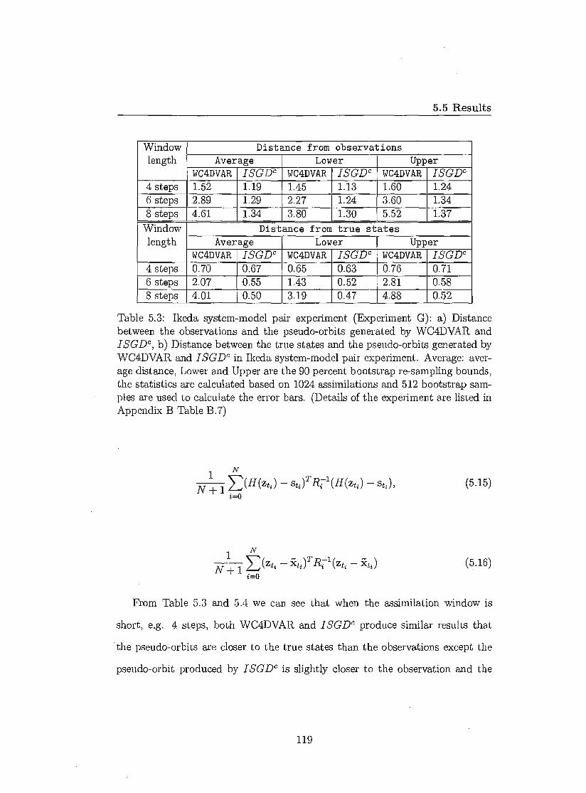
5.5 Results
Window length
Distance from observations Average Lower Upper
WC4DVAR ISGDe WC4DVAR ISGDe WC4DVAR ISGDe 4 steps 1.52 1.19 1.45 1.13 1.60 1.24 6 steps 2.89 1.29 2.27 1.24 3.60 1.34 8 steps 4.61 1.34 3.80 1.30 5.52 1.37
Window length
Distance from true states Average Lower Upper
WC4DVAR ISGDe WC4DVAR ISGDe WC4DVAR ISGDe 4 steps 0.70 0.67 0,65 0.63 0.76 0.71. 6 steps 2.07 0.55 1.43 0.52 2.81 0.58 8 steps 4.01 0.50 3.19 0.47 4.88 0.52
Table 5.3: Ikeda system-model pair experiment (Experiment G): a) Distance between the observations and the pseudo-orbits generated by WC4DVAR and ISGDe, b) Distance between the true states and the pseudo-orbits generated by WC4DVAR and ISGDe in Ikeda system-model pair experiment. Average: aver-age distance, Lower and Upper are the 90 percent bootstrap re-sampling bounds, the statistics are calculated based on 1024 assimilations and 512 bootstrap sam-ples are used to calculate the error bars. (Details of the experiment are listed in Appendix B Table B.7)
( H - sti )TR71 (H(zti ) - SO, (5.15)
- ROT Ri (zt, - Rt,) (5.16)
From Table 5.3 and 5.4 we can see that when the assimilation window is
short, e.g. 4 steps, both WC4DVAR and ISGDe produce similar results that
the pseudo-orbits are closer to the true states than the observations except the
pseudo-orbit produced by ISGDe is slightly closer to the observation and the
119
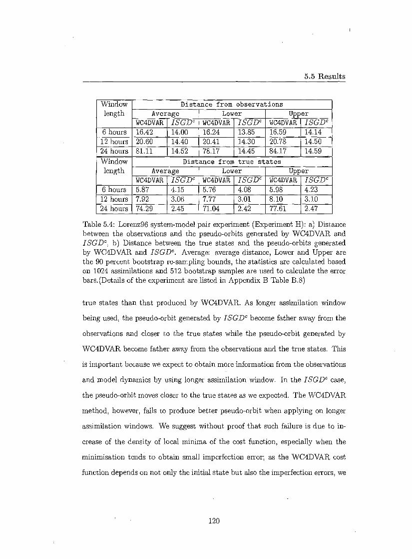
5.5 Results
Window length
Distance from observations Average Lower Upper
WC4DVAR ISCDc WC4DVAR ISCDc WC4DVAR ISG.Dc 6 hours 16.42 14.00 16.24 13.85 16.59 14.14 12 hours 20.60 14.40 20.41 14.30 20.78 14.50 24 hours 81.11 14.52 78.17 14.45 84.17 14.59 Window length
Distance from true states Average Lower Upper
WC4DVAR ISG.De WC4DVAR ISG.Dc WC4DVAR ISGDC 6 hours 5.87 4.15 5.76 4.08 5.98 4.23 12 hours 7.92 3.06 7.77 3.01 8.10 3.10 24 hours 74.29 2.45 71.04 2.42 77.61 2.47
Table 5.4: Lorenz96 system-model pair experiment (Experiment H): a) Distance between the observations and the pseudo-orbits generated by WC4DVAR and ISGDa, b) Distance between the true states and the pseudo-orbits generated by WC4DVAR and ISGDc. Average: average distance, Lower and Upper are the 90 percent bootstrap re-sampling bounds, the statistics are calculated based on 1024 assimilations and 512 bootstrap samples are used to calculate the error bars.(Details of the experiment are listed in Appendix B Table B.8)
true states than that produced by WC4DVAR. As longer assimilation window
being used, the pseudo-orbit generated by ISGD° become father away from the
observations and closer to the true states while the pseudo-orbit generated by
WC4DVAR become father away from the observations and the true states. This
is important because we expect to obtain more information from the observations
and model dynamics by using longer assimilation window. In the ISGIY case,
the pseudo-orbit moves closer to the true states as we expected. The WC4DVAR
method, however, fails to produce better pseudo-orbit when applying on longer
assimilation windows. We suggest without proof that such failure is due to in-
crease of the density of local minima of the cost function, especially when the
minimisation tends to obtain small imperfection error; as the WC4DVAR cost
function depends on not only the initial state but also the imperfection errors, we
120
5.5 Results
are unable to plot the cost function against the initial state to demonstrate the
appearance of local minimums. To support our suggestion, however, we apply the
WC4DVAR method on different realizations of observations of the true states.
If the WC4DVAR cost function does not have multiple local minimums, we ex-
pect that the pseudo-orbit produced by WC4DVAR should not varies much for
different realizations of observations. Table 5.5 and 5.6, shows the standard devi-
ation of both middle point and end point of the pseudo-orbits , The WC4DVAR
method is compared with ISG.Dc method. It appears that for ISG.Dc method the
standard deviation does not vary much for different length of assimilation win-
dows while for WC4DVAR method different realization of observations effect the
results more when the assimilation window becomes larger, which also indicates
that more local minimums appears.
5.5.2 Evaluate ensemble nowcast
In this section we compare nowcast performance of the three ensemble methods
based on ISCDc with the Inverse Noise ensemble. For the purpose of illustration,
we call the Inverse Noise ensemble Method I; the ensemble formed by dressing the
end point of the pseudo-orbit with Gaussian distribution Method II; the ensemble
formed by perturbing the image of the second last component with imperfection
error Method III and the ensemble formed by perturbing the pseudo-orbit and
applying IS'GDc Method IV. The three ensemble methods based on ISGDc are
introduced and discussed in section 5.4. The Inverse Noise ensemble is formed by
sampling the inverse noise distribution and adding onto the observations (details
1We expect the middle point provides better estimate of the model state than the end point as the end point only has information from the past, the middle point has information of both past and future.
121
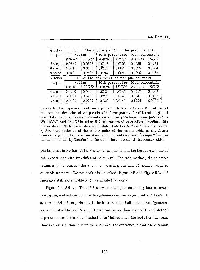
5.5 Results
Window length
STD of the middle point of the pseudo-orbit Median 10th percentile 90th percentile
WC4DVAR ISG.Dc WC4DVAR ISCDc WC4DVAR ISGDc 4 steps 0.0153 0.0155 0.0113 0.0105 0.0259 0.0274 6 steps 0.0271 0.0126 0.0121 0.0087 0.0595 0.0264 8 steps 0.0431 0.0126 0.0242 0.0086 0.0905 0.0262
Window length
STD of the end point of the pseudo-orbit Median 10th percentile 90th percentile
WC4DVAR ISCIY WC4DVAR ISCDc WC4DVAR ISGDe 4 steps 0.0260 0.0301 0.0124 0.0147 0.0417 0.0407 6 steps 0.0369 0.0296 0.0228 0.0147 0.0841 0.0407 8 steps 0.0590 0.0299 0.0363 0.0147 0.1294 0.0406
Table 5.5: Ikeda system-model pair experiment, following Table 5.3: Statistics of the standard deviation of the pseudo-orbits' components for different lengths of assimilation window, for each assimilation window, pseudo-orbits are produced by WC4DVAR and ISGDc based on 512 realizations of observations. Median, 10th percentile and 90th percentile are calculated based on 512 assimilation windows. a) Standard deviation of the middle point of the pseudo-orbit, as the chosen window length contain even numbers of components we treat (Length/2) - 1 as the middle point; b) Standard deviation of the end point of the pseudo-orbit.
can be found in section 4.3.1). We apply each method in the Ikeda system-model
pair experiment with two different noise level. For each method, the ensemble
estimate of the current states, i.e. nowcasting, contains 64 equally weighted
ensemble members. We use both &ball method (Figure 5.5 and Figure 5.6) and
ignorance skill score (Table 5.7) to evaluate the results.
Figure 5.5, 5.6 and Table 5.7 shows the comparison among four ensemble
nowcasting methods in both Ikeda system-model pair experiment and Lorenz96
system-model pair experiment. In both cases, the c-ball method and ignorance
score indicates Method IV and III performs better than Method II and Method
II performances better than Method I. As Method I and Method II use the same
Gaussian distribution to form the ensemble, the difference is that the ensemble
122
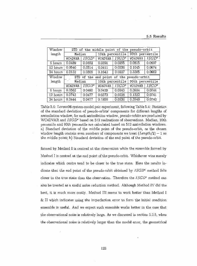
5.5 Results
Window length
STD of the middle point of the pseudo-orbit Median 10th percentile 90th percentile
WC4DVAR ISCDc WC4DVAR I SG.Dc WC4DVAR ISGDc 6 hours 0.0489 0.0402 0.0391 0.0295 0.0815 0.0697 12 hours 0.0540 0.0314 0.0411 0.0236 0.1045 0.0674 24 hours 0.2132 0.0309 0.1642 0.0227 0.3505 0.0662 Window length
STD of the end point of the pseudo-orbit Median 10th percentile 90th percentile
WC4DVAR ISG_Dc WC4DVAR ISGDe WC4DVAR ISCDc 6 hours 0.0563 0.0480 0.0429 0.0243 0.0934 0.0744 12 hours 0.0743 0.0477 0.0573 0.0238 0.1332 0.0741 24 hours 0.2444 0.0477 0.1859 0.0236 0.3949 0.0740
Table 5.6: Lorenz96 system-model pair experiment, following Table 5.4: Statistics of the standard deviation of pseudo-orbits' components for different lengths of assimilation window, for each assimilation window, pseudo-orbits are produced by WC4DVAR and ISG.Dc based on 512 realizations of observations. Median, 10th percentile and 90th percentile are calculated based on 512 assimilation windows. a) Standard deviation of the middle point of the pseudo-orbit, as the chosen window length contain even numbers of components we treat (Length12)- 1 as the middle point; b) Standard deviation of the end point of the pseudo-orbit.
formed by Method I is centred at the observation while the ensemble formed by
Method I is centred at the end point of the pseudo -orbit. Whichever wins merely
indicates which centre tend to be closer to the true state. Here the results in-
dicate that the end point of the pseudo-orbit obtained by ISCDc method falls
closer to the true state than the observation. Therefore the ISG.Dc method can
also be treated as a useful noise reduction method. Although Method IV did the
best, it is much more costly. Method III seems to work better than Method I
& II which indicates using the imperfection error to form the initial condition
ensemble is useful. And we expect such ensemble works better in the case that
the observational noise is relatively large. As we discussed in section 5.2.5, when
the observational noise is relatively larger than the model error, the geometrical
123
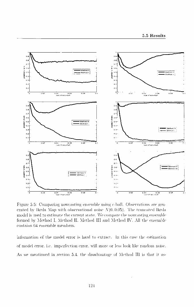
0 1 0.02 0.08
0.08 0 1
00
0.02 0.08 01
1
0.9
0.8
0.7
O.6
0.4
0.3
0.2
0.1
1
0.9
0.8
0.7
I 0.6
. 5 0.5
0.4
Method III Method II
0.04 0.06 size of epe-bell
Method IV Method II
0.02
0.9
0.8
0.7
8 0.6
S 0.5
0.4 LLL
0.3
0.2
0.1
00
Method IV Method III
O8
07
5 0.6
8 0.5
k 0 4
5.5 Results
1
0.9
0.8
0 7
S 0.6
Method II - Method I
0.3
0.2
0.1
00
0.02 0.04 0.06 size of eps-ball
0.08
01
eeesee Method IV Method I
0.3
0.2
0.1
00
0.02 0.04 0.06 0.08 01 size of eps-bell
Figure 5.5: Comparing nowcasting ensemble using &ball. Observations are gen-erated by Ikeda Map with observational noise N(0, 0.05). The truncated Ikeda model is used to estimate the current state. We compare the nowcasting ensemble formed by Method I, Method II, Method III and Method IV. All the ensemble contains 64 ensemble members.
information of the model error is hard to extract. In this case the estimation
of model error, i.e. imperfection error, will more or less look like random noise.
As we mentioned in section 5.4, the disadvantage of Method III is that it as-
124
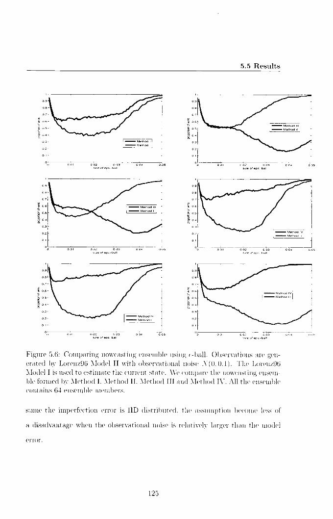
0.01 0.02 0.03 size of eps-ball
0.04 0 05
1 0.9
0.8
0.7
I 0.6
0.9
0.8
0.7
0.6
0.5
0.4
0.3
0.2
0.1
0.5
0.4
0.3
0.2
0.1
00
O 0.01 0.01 0.05 0.04 0.04 0.05 0.02 0.03
size of eps-bell 0.02 003
size of °es Gall
1 0.9
0.8
0.7
§ 0.6
0.9
0.8
0.7
0.6
0.5
0.4
0.3
0.2
0.1
0.5
0.4
0.3
0.2
0.1
0 0.05 0.04 00
00 0.01 0.04 0.05 0.02 0.03
sae of eps-bell 0.02 0.03 size of eps-ball
5.5 Results
0.9
0.8
0.7
I 0.6 15 15 I 0.5
OA 1 0.5
0.4
0.3 0.3 Method I
0.2 0.2
0.1 0.1
0.01
0.02 0.03
0.04
0.05 0
size of fps-ball
Figure 5.6: Comparing nowcasting ensemble using f-ball. Observations are gen-erated by Lorenz96 Model II with observational noise N(0, 0.1). The Lorenz96 Model I is used to estimate the current state. We compare the nowcasting ensem-ble formed by Method I, Method II, Method III and Method IV. All the ensemble contains 64 ensemble members.
sume the imperfection error is IID distributed, the assumption become less of
a disadvantage when the observational noise is relatively larger than the model
error.
125
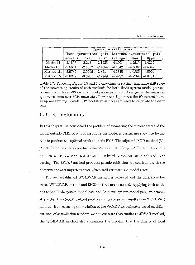
5.6 Conclusions
Ignorance skill score Ikeda system-model pair Lorenz96 system-model pair Average Lower Upper Average Lower Upper
Method I -2.1863 -2.248 -2.1233 -4.4901 -4.5519 -4.4252 Method II -2.5351 -2.5857 -2.4854 -4.6042 -4.6682 -4.5349 Method III -2.9782 -3.0665 -2.891 -4.6345 -4.6886 -4.5966 Method IV -3.0267 -3.0981 -2.9249 -4.9227 -4.9964 -4.8181
Table 5.7: Following Figure 5.5 and 5.6 experiments setting, Ignorance skill score of the nowcasting results of each methods for both Ikeda system-model pair ex-periment and Lorenz96 system-model pair experiment. Average: is the empirical ignorance score over 1024 nowcasts , Lower and Upper are the 90 percent boot-strap re-sampling bounds, 512 bootstrap samples are used to calculate the error bars.
5.6 Conclusions
In this chapter, we considered the problem of estimating the current states of the
model outside PMS. Methods assuming the model is perfect are shown to be un-
able to produce the optimal results outside PMS. The adjusted ISGD method (50)
is also found unable to produce consistent results. Using the ISGD method but
with certain stopping criteria is then introduced to address the problem of now-
casting. The ISCDc method produces pseudo-orbit that are consistent with the
observations and imperfect error which well estimate the model error.
The well established WC4DVAR method is reviewed and the differences be-
tween WC4DVAR method and ISGD method are discussed. Applying both meth-
ods to the Ikeda system-model pair and Lorenz96 system-model pair, we demon-
strate that the ISCDc method produces more consistent results than WC4DVAR
method. By measuring the variation of the WC4DVAR estimates based on differ-
ent sizes of assimilation window, we demonstrate that similar to 4DVAR method,
the WC4DVAR method also encounters the problem that the density of local
126

5.6 Conclusions
minima increases as the length of assimilation window increases.
Three methods are introduced to form the initial condition ensemble based on
the pseudo-orbit provided by ISGDc method. Using the information of imper-
fection error are found to be useful to produce better initial condition ensemble.
Forming the ensemble by applying ISG.Dc on perturbed pseudo-orbit are found
to produce the best initial condition ensemble among these three methods.
127

Chapter 6
Forecast and predictability
outside P S
In this penultimate chapter we discuss how to produce better forecast based on
the initial condition ensemble given the fact that our model is imperfect. By
showing the results in the Ikeda system-model pair experiment, we demonstrate
first that forecast with relevant adjustment, which could be obtained from the
imperfection error (see section 5.2.3), can produce better forecast than ignoring
the existence of model error. Secondly we discuss how to interpret predictability
outside PMS. Traditional ways of evaluating the predictability of one model,
Lyapunov exponents and doubling time for example, provide the information of
error growth but they implicitly assume the model is perfect. Outside PMS these
measurements would systematically overestimate the predictability. We suggest
using the probability forecast skill to interpret the predictability. Such forecast
skill not only depends on the system, and model, and observation method but
also depends on the way that initial conditions are formed and forecasts are
128

6.1 Forecasting using imperfect model
determined from the ensemble.
6.1 Forecasting using imperfect model
6.1.1 Problem setting up
We set up the forecast problem in the imperfect model scenario following (50).
As in section 5.1, the trajectory of system states, Rt , t = —n, 0, ..., ml where
Rt e Rth , where Rh is the state space of the system, is governed by the nonlinear
evolution operator F , i.e. 5444 = P(5.ct). An observation s t of the system state Rt
at time t is defined by s t = h(51t)4-ri t where s t e 0, Th represents the observational
noise, which we assume is IID distributed, and h(.) is the observation operator,
which projects the system state into the observation space 0. For simplicity, we
take h(.) to be the identity. Let the model be x t+i = F(xt ), where x t E M, M
is the model state space. Assume the system state k can also be projected into
the model state space by a projection operator g(•), i.e. x = g(X). In general,
we don't know the property of this projection operator, we don't know even if
exists. We are just going to assume that it maps the states of the system
into somehow relevant states in the model. For the purposes of illustration and
simplicity, unless otherwise stated, we assume g(.) is one-to-one identity. Our
aim is to forecast the future model states x t , t = 1, ..., n1 given the model and
the previous and current observations s t , t = —n, 0. Chapter 3 and Chapter
5 have discussed methods to estimate the current state using ensemble. In the
following sections, we will treat the ensemble for the current states as the initial
condition ensemble and use them to forecast the future states x t , t = 1, ..., nf.
129

6.1 Forecasting using imperfect model
The experimental results discussed in this section will based on the Ikeda
system-model pair, i.e treat the Ikeda Map as the system and the truncated Ikeda
Map as the model. Details of this system-model pair can be found in Section 5.1
and 2.4.
6.1.2 Ignoring the fact that the model is wrong .
Given an initial condition ensemble, the simplest way to produce the forecast
ensemble is to iterate the initial condition ensemble forward by•the model, we
call this the direct forecast. Unfortunately no matter how good the initial con-
dition ensembles are, by simply iterating them forward the forecast ensembles
are expected to move far away from the observations eventually. This failure
of producing a relevant forecast results from ignoring the fact that the model is
imperfect. Usually the invariant measure of the system in the model space and
that of the model are rather different, and iterations of the initial condition un-
der the model will, however, only approach the model attractor (if there is one)
eventually, which essentially cause the irrelevance of the forecast.
6.1.3 Forecast with model error adjustment
As discussed in section 5.2, a system trajectory provides a pseudo-orbit of the
model instead of a model trajectory in the model space. The mismatch R t+i —
F(Rt ), i.e. the model error dh, distinguishes a system trajectory from being a
model trajectory. Forecasting by iterating the initial condition ensemble forward
by the model ignores the existence of model error. Given an initial condition
ensemble at time 0, the ideal forecast at time 1 would be obtained by adjusting
130
6.1 Forecasting using imperfect model
the iteration of the initial condition ensemble with the corresponding model error.
If one has a large sample of historical model errors -P j l, these could be used
to improve the forecasting. One could, for example, adjust the iterations of initial
condition ensemble with random draws from the set of relevant historical model
errors (79). Let the initial condition ensemble be xio ,i = 1, ... Nens where Nens is
the number of ensemble members. The forecast ensemble member at lead time
t is then given by xit = F(x1_ 1 ) Cit where Cti is random drawn from the set of
historical model error. we call this the forecast with random adjustment. This
method is equivalent to transferring the deterministic model F to a stochastic
model by adding the dynamical noise term C t . And this method assumes that
the model error is IID distributed when usually it is not the case.
Model error is usually correlated, for example see Figure 5.1. Randomly
drawing from the set of global historical model error discards the geometrical
information about model error. Another approach by using historical model
error that doesn't discard geometrical information is to employ a local analogue
model to determine the adjustments fit. For each model error (Di , it corresponds
to two sequential states x3 and 5cj+1 as c.:.7' ; = — F(Ri ). To construct Ct , we
can first find K nearest neighbours of xi from the historical set {ic; } and record
their corresponding (.7.7j , we then randomly choose one model error from the K
CZ) to be Cti . We call this method forecast with analogue adjustment. There are
many other analogue models one can use (details of analogue models can be found
in Section 2.5), our interest here is not finding a better analogue model but to
demonstrate that by extracting information from the model errors the forecast
performance can be improved.
• For computational reasons, we illustrate both methods taking only one ad-
131

6.1 Forecasting using imperfect model
justment for each ensemble member xt. Note that in future work, one could
sample more than one from the set of historical model error or from the K local
model error (70). Taking large samples will be more useful, but will lead to ex-
ponentially growing ensemble size, which is interesting but beyond the scope of
current thesis.
The experiment results discussed below are based on two different initial con-
dition ensembles. One is inverse noise (see section 4.3.1), which is a computation-
ally cheap and easy way to form the initial condition ensemble but which ignores
the information of the dynamics. The other is the dynamical consistent ensemble
(see section 3.6), in our experiment the ensemble members are consistent with
the system dynamics and a segment of observations, si, i = —5, —4, ..., O. In the
imperfect model scenario, such initial condition ensemble is not achievable as the
system dynamics is unknown. We use such "perfect" initial condition ensemble
as an example of the best initial condition ensemble one might hope to achieve.
Results shown below demonstrate that forecasting with the adjustment of model
error improves the forecast performance in both cases.
Figure 6.1 shows four examples of the one step forecast ensemble in the model
state space when the initial condition ensemble is formed by inverse noise. In all
the examples, forecasting with random adjustment produces ensemble members
with too much spread. In panel (a), forecasting were made in a place where
the model error is very small, which makes the difference between direct forecast
and forecast with analogue adjustment very small. Panel (b) shows an example
where the model error is small but not negligible, direct forecast ensemble fails
to capture the true state to a slight extent. Panel (c) and (d) are cases that
the model error is moderate and relatively large, in both cases direct forecast
132
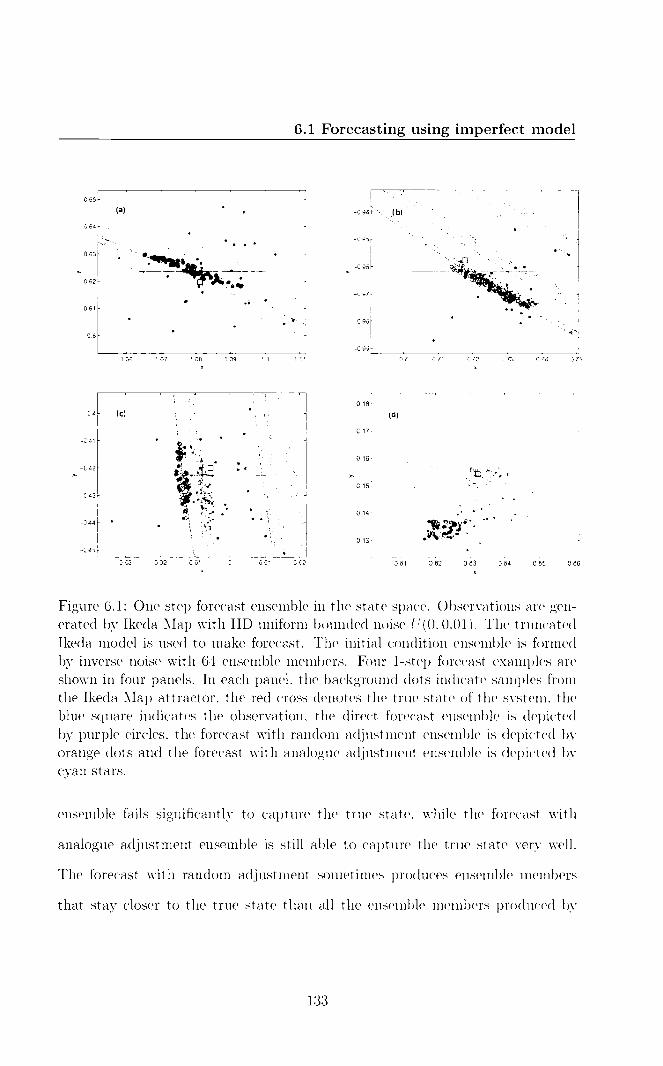
0.81 0.82 0.83 0.84 0.85 0.88
07 0 7 , 0 73 0 74
0.18
0.17
0.16
0.15
0.14
0.13
1 06 1 07 1.08 1.09 1.1
-0 4
-041
-042
-0 43
-0 44
-0 45
-0.03 -0.02 -am 0 02 .
'
•
(C)
6.1 Forecasting using imperfect model
Figure 6.1: One step forecast ensemble in the state space. Observations are gen-erated by Ikeda Map with IID uniform bounded noise U(0, 0.01). The truncated Ikeda model is used to make forecast. The initial condition ensemble is formed by inverse noise with 64 ensemble members. Four 1-step forecast examples are shown in four panels. In each panel, the background dots indicate samples from the Ikeda Map attractor, the red cross denotes the true state of the system, the blue square indicates the observation, the direct forecast ensemble is depicted by purple circles, the forecast with random adjustment ensemble is depicted by orange dots and the forecast with analogue adjustment ensemble is depicted by cyan stars.
ensemble fails significantly to capture the true state, while the forecast with
analogue adjustment ensemble is still able to capture the true state very well.
The forecast with random adjustment sometimes produces ensemble members
that stay closer to the true state than all the ensemble members produced by
133

6.1 Forecasting using imperfect model
direct forecast.
Figure 6.2 shows the comparison between the three methods discussed above
using the c-ball test at different lead times (Details of c-ball method can be found
in Section 3.7). It appears that forecasts with analogue adjustment almost always
outperform the direct forecasts for different lead times and different sizes of e-
b all . At lead time 1 and 2, direct forecasts outperform the forecasts with random
adjustment no matter what the size of c-ball is. At lead time 4, the proportion
of wins for these two methods are close when the diameter of c-ball is less than
0.03, beyond 0.03 direct forecast wins. At lead time 8 and lead time 16, however,
forecast with random adjustment outperforms the direct forecast. The reason of
direct forecast winning at short lead time and losing at longer lead time is that
at short lead time although the direct forecast may not capture the true state,
the forecast ensemble members are still stay relatively close to the true state. For
longer lead time, a direct forecast ensemble is not only unable to capture the true
state but also further way from the true state.
Following Figure 6.1, Figure 6.3 shows the same four examples of the one step
forecast ensemble but based on the initial condition ensemble that is a dynamical
consistent ensemble in the state space. Forecasts with random adjustment still
produce ensemble members with too much spread. Although the initial conditions
are consistent with both observations and system dynamics, the direct forecast
fails to capture the true state with the appearance of model error. Forecast with
analogue adjustment ensemble members not only cover the true state but also lie
closer to the relevant system attractor.
Following Figure 6.2, Figure 6.4 shows the c-ball test for the three forecasting
methods at different lead time where the initial condition ensemble is formed by
134

0.00 0.0e
4 ° °
°
0 Oa 0 06 0 00 oo so 01 0 00—bealt
°-' oe °
0 1
6.1 Forecasting using imperfect model
Figure 6.2: Following Figure 6.1 experiment setting, compare forecast ensemble using e-ball. Direct forecasts are compared with forecasts with random adjust-ment (left) and forecasts with analogue adjustment (right). The initial condition ensemble is formed by inverse noise with 64 ensemble members. For each forecast method, 2048 forecasts are made. Each row shows the comparison for different lead time. First row denotes lead time 1, second lead time 2, third lead time 4, forth lead time 8 and fifth lead time 16.
135

081 0 82 0.83 084 0.85 086
-0.94
- 0.95
-0.96
- 0.97
-0.98
-0.99
0.7 0.71 0.73 0.74 0.75
ale
0.17
0.16
0.15
0.14
0.13
1.06 1.07 1.09 1.1 111
-0.03 -0 02 -0.01 001 0.02
6.1 Forecasting using imperfect model
Figure 6.3: Following Figure 6.1 one step forecast ensemble in the state space. The initial condition ensemble is formed by dynamical consistent ensemble with 64 ensemble members.
a dynamical consistent ensemble. The results are almost the same as seen in
Figure 6.2 did. Comparing with Figure 6.2, the advantage of using adjustment
at longer lead time becomes more obvious as the dynamical consistent initial
conditions are more concentrated than inverse noise ensemble which makes the
forecast ensemble less likely to capture the true state using a direct forecast.
Figure 6.1 and Figure 6.3 have compared the results of three forecasting meth-
ods in the state space at lead time 1. And Figure 6.2 and Figure 6.4 compare their
forecast performance at different lead times by looking at the probability mass
136

6.1 Forecasting using imperfect model
Figure 6.4: 6.4: Comparing forecast ensemble using e-ball. Observations are generated by Ikeda Map with IID uniform bounded noise U(0, 0.01). The truncated Ikeda model is used to make forecast. The initial condition ensemble is formed by dynamical consistent ensemble with 64 ensemble members. Each row of pictures shows the comparison for different lead time. First row denotes lead time 1, second lead time 2, third lead time 4, forth lead time 8 and fifth lead time 16.
137
6.1 Forecasting using imperfect model
around the true state. We now look at their forecast performance at different lead
times using the ignorance score. Following section 4.3.2, we first transform the
forecast ensemble into a probability distribution by standard kernel dressing, and
we use the historical observations for a climatology which is blended with forecast
distribution generated by forecast ensemble. we evaluate the final forecast proba-
bility distribution by the ignorance score. Figure 6.5 plots the ignorance score of
three forecasting methods for different lead times. In panel (a) the forecasts are
based on an inverse noise initial condition ensemble. In panel (b) the forecasts
are based on a dynamical consistent initial condition ensemble. In both cases,
the forecasts with random adjustment appears slightly better than direct fore-
cast, and forecasts with analogue adjustment outperforms the other two methods
significantly. Panel (c) combines the panel (a) and panel (b) in order to compare
the difference between different initial condition ensembles. From panel (c), it
appears that using a dynamical consistent ensemble for the initial condition is
only slightly better than using inverse noise ensemble for both direct forecast and
forecasting with random adjustment, while for the forecast with analogue adjust-
ment a dynamical consistent ensemble initial condition can improve the forecast
perform significantly which indicates that the information of the initial condition
is well maintained.
From Figure 6.2, 6.4 and 6.5, it seems that c-ball test and ignorance score
do not indicate a single best approach in the case of comparing direct forecast
and forecast with random adjustment, especially at short lead times. Comparing
these two methods by 6-ball test, the proportion of wins of direct forecast is never
smaller than that of forecast with random adjustment for any size of 6-ball at lead
time 1 and 2. By comparing the ignorance score, however, forecasts with random
138
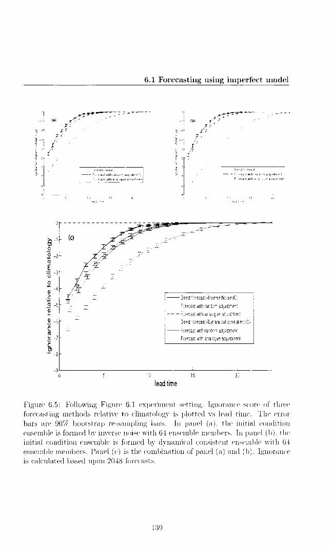
0
- Direct forecast - Forecast with random adjustment Forecast with analogue adjustment
-5
9
Direct forecast - Forecast with randan adwalment Forecast with analogue achustrnent
-Et
10 15 lead lane
so 5 20
- Direct forecast (Inverse Noise IC) — Forecast with random adjustment — Forecast with analogue adjustment Direct forecast (Dynamical consistent IC) — Forecast with random adjustment
Forecast with analogue adjustment
1n 15 20 lead time
5
-7 C rn
-90
-
6.1 Forecasting using imperfect model
0 5 10 15
20 Lead t!rne
Figure 6.5: Following Figure 6.1 experiment setting, Ignorance score of three forecasting methods relative to climatology is plotted vs lead time. The error bars are 90% bootstrap re-sampling bars. In panel (a), the initial condition ensemble is formed by inverse noise with 64 ensemble members. In panel (b), the initial condition ensemble is formed by dynamical consistent ensemble with 64 ensemble members. Panel (c) is the combination of panel (a) and (b). Ignorance is calculated based upon 2048 forecasts.
139
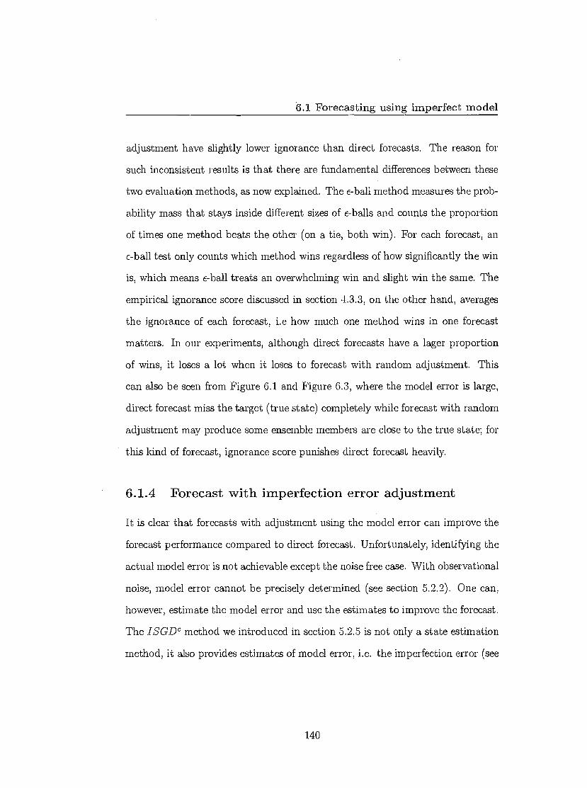
G.1 Forecasting using imperfect model
adjustment have slightly lower ignorance than direct forecasts. The reason for
such inconsistent results is that there are fundamental differences between these
two evaluation methods, as now explained. The e-ball method measures the prob-
ability mass that stays inside different sizes of e-balls and counts the proportion
of times one method beats the other (on a tie, both win). For each forecast, an
&ball test only counts which method wins regardless of how significantly the win
is, which means e-ball treats an overwhelming win and slight win the same. The
empirical ignorance score discussed in section 4.3.3, on the other hand, averages
the ignorance of each forecast, i.e how much one method wins in one forecast
matters. In our experiments, although direct forecasts have a lager proportion
of wins, it loses a lot when it loses to forecast with random adjustment. This
can also be seen from Figure 6.1 and Figure 6.3, where the model error is large,
direct forecast miss the target (true state) completely while forecast with random
adjustment may produce some ensemble members are close to the true state; for
this kind of forecast, ignorance score punishes direct forecast heavily.
6.1.4 Forecast with imperfection error adjustment
It is clear that forecasts with adjustment using the model error can improve the
forecast performance compared to direct forecast. Unfortunately, identifying the
actual model error is not achievable except the noise free case. With observational
noise, model error cannot be precisely determined (see section :5.2.2). One can,
however, estimate the model error and use the estimates to improve the forecast.
The ISCDc method we introduced in section 5.2.5 is not only a state estimation
method, it also provides estimates of model error, i.e. the imperfection error (see
140

6.1 Forecasting using imperfect model
Section 5.2). In this section we consider using the imperfection error to adjust
the forecast and compare with direct forecasts. The experiment results discussed
below are based on initial condition ensemble obtained by inverse noise 1. .
Figure 6.6 shows six examples of the one step forecast ensemble in the state
space, the initial condition ensemble is formed by inverse noise. Instead of using
the actual model error we use the model imperfection error obtained from the
ISGDC method to adjust the forecast. In all examples, forecasts with random
adjustment still produce ensemble members with too much spread. Similar to
Figure 6.1, the first 4 panels present the four cases where the model error is very
small, small, moderate and large. Forecasts with analogue adjustment outperform
the direct forecast as long as the model error is not negligible. Panel (e) shows an
example where the model error is small but the forecast with analogue adjustment
ensemble is unable to capture the true state. This failure occurs because the
model error in this case is overestimated by the imperfection error. Panel (f)
shows an opposite example where forecasts with analogue adjustment did not
capture the true state because the model error in this case is underestimated by
the imperfection error. Figure 6.7 shows the comparison between three methods
via &ball method (see section 3.7) at different lead time, the forecast adjustment
is obtained from the imperfection error instead of model error. Similar to the
adjustment using model error, the forecasts with analogue adjustment almost
always outperform the direct forecast for different lead time and different sizes of
c-ball. Direct forecasting outperforms the forecasts with random adjustment at
short lead times while underperforms at longer lead times. As the result of using
'dynamical consistent ensemble is not employed this time since if method can improve the forecast based on inverse noise it is expected to do so for other initial condition ensemble and it might be too costly to form an dynamical consistent ensemble in practice
141

0 29
C 26
0 27
C 26
0 25
0 24
0 02
001
-CCI
-0 02
-003
037 025
0 24 0 36
023 ,,, 0 35
0 22 034
021 0 33
02 0 32
6.1 Forecasting using imperfect model
005 aos 0.07 008 009 0 1 13 1.31 1 32 133 134 135
- 0 05
-0 06
- 0 07
." -0 08
- 0 09
-0 1
-0 4
- 0 41
- 0 42
- 0 43
- 044
- 0 45
-003 -0.02 -0 01x 0 061 0.02 1 36 1 09 1 12 1 13
1.34 1 35 1 36 1 37 1 30 1 39 116 1 17 1 181 19 x 1.2 1.21
Figure 6.6: Following Figure 6.1, six 1-step forecast examples are plotted in the state space. Here the adjustment is obtained from imperfection error instead of model error.
142

0 2
0.8
0.09 0 00 0.00 017. 01 000-8011
V.-
---0—:,=7—"""---1 I
6.1 Forecasting using imperfect model
Figure 6.7: Following Figure 6.2, comparing three forecast ensemble results using &ball. Here the adjustment is obtained from imperfection error instead of model error.
imperfection error, forecasts using analogue adjustment outperform the direct
forecast less significantly than using the actual model error. Figure 6.8 plots the
ignorance score of three forecasting methods for different lead time. Similar to
143
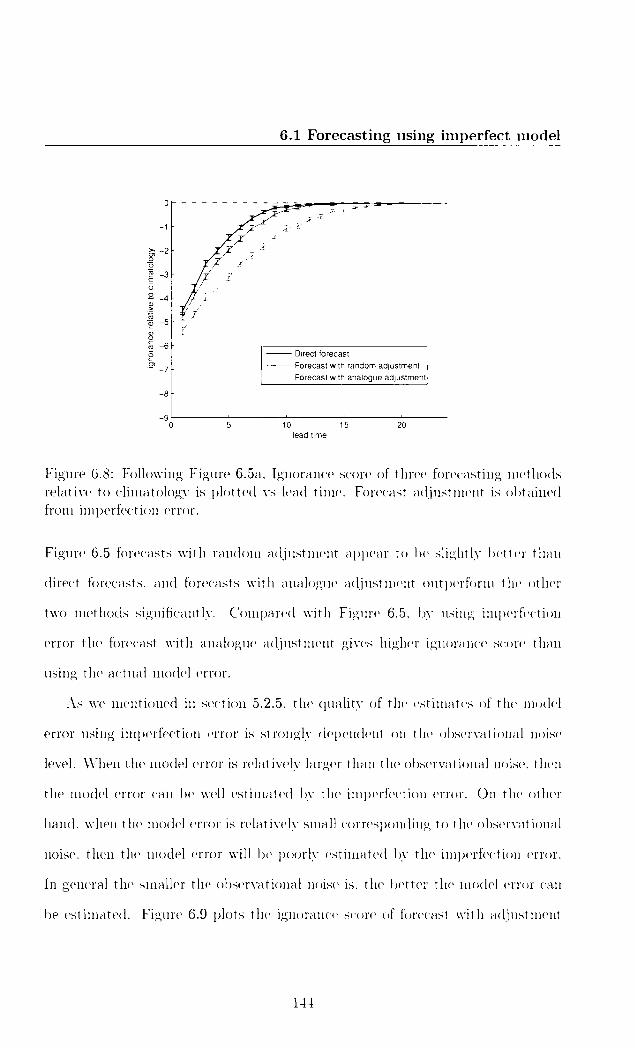
Direct forecast Forecast with random adjustment Forecast with analogue adjustment
6.1 Forecasting using imperfect model
5
10 15
20 lead time
Figure 6.8: Following Figure 6.5a, Ignorance score of three forecasting methods relative to climatology is plotted vs lead time. Forecast adjustment is obtained from imperfection error.
Figure 6.5 forecasts with random adjustment appear to be slightly better than
direct forecasts, and forecasts with analogue adjustment outperform the other
two methods significantly. Compared with Figure 6.5, by using imperfection
error the forecast with analogue adjustment gives higher ignorance score than
using the actual model error.
As we mentioned in section 5.2.5, the quality of the estimates of the model
error using imperfection error is strongly dependent on the observational noise
level. When the model error is relatively larger than the observational noise, then
the model error can be well estimated by the imperfection error. On the other
hand, when the model error is relatively small corresponding to the observational
noise, then the model error will be poorly estimated by the imperfection error.
In general the smaller the observational noise is, the better the model error can
be estimated. Figure 6.9 plots the ignorance score of forecast with adjustment
0
E
9
•
-4
11
•
-5
O
c7, -6 O
c2, —7
-8
-9
144

- U(0,0.01) - U(0,0.02) - U(0.0.04)
6.1 Forecasting using imperfect model
- U(0,0.01) - U(0.0.02) U(0,0.04)
-8 6
0 5 10 15 0 load Om
10 15 Mad ti*
Figure 6.9: Ignorance score of forecast with adjustment where the adjustment is generated from the observations with different noise level. The initial condition ensemble is formed by inverse noise with fixed noise level U(0, 0.01) so that the observations with different noise level only affect the imperfection error. The error bars are 90% bootstrapped error bars. In panel a, the forecast is made by random adjustment; in panel b, the forecast is made by analogue adjustment
where the imperfection error is produced of different noise levels. It appears
that forecasts with random adjustment are not affected much by having higher
observational noise. Doubling the observational noise, however, decreases the
forecast performance of using analogue adjustment.
Overall, we conclude that forecasting with adjustments can improve the fore-
cast performance from direct forecast as the adjustment is able to account the
model inadequacy partially. The adjustments can be obtained from estimates
of the model error. Such estimates can be obtained for example using ISGIY
method. Forecasts with random adjustment ignores the geometric information
of model error by assuming it is IID distributed. Forecast with analogue adjust-
ment extracts such information and as a result, outperforms forecast with random
adjustment and direct forecast significantly.
145
6.2 Predictability outside PMS
6.2 Predictability outside PMS
If the dynamics of a deterministic system are completely understood and the ex-
act initial state is observed, then there is no limit to predictability and the future
holds no surprises. When there is uncertainty in the initial condition, sensitive
dependence on initial conditions restricts our ability to predict the future. The
well known Lyapunov exponents (3; 22; 68) measures the predictability by cal-
culating the average exponential uncertainty growth rates. Lorenz (62) discussed
using finite time Lyapunov exponents to measure the predictability of high di-
mensional atmospheric model. The weakness of using Lyapunov exponents is
revealed by Smith et al (82) by comparing q-pling times which reflects the time
of error growth directly. The q-pling times are used to measure the predictability
by directly quantifying the time at which initial uncertainty increases by a factor
of q.
Outside PMS, there is not only uncertainty in the initial condition but also
uncertainty in the dynamics. Measuring the predictability with the assumption
that the model is perfect will simply overestimate the predictability. Without
knowing the true state of the system, q-pling times can be used to estimate the
uncertainty doubling (quadrupling, etc) time based on the sequence of observa-
tions. Knowing a particular q-pling time, however, from which the uncertainty
growth rate can not be simply inferred, as discussed in Smith(1996), the rela-
tion re 27-g may not hold. We suggest that outside PMS one could define
predictability being lost when the forecast adds no new information to the cli-
matology (82). In practice, this is to say that the predictability is lost when the
forecast skill score relative to climatology is arguably zero. Lyapunov Exponents
146
6.2 Predictability outside PMS
and q-pling time are discussed in Section 6.2.1 and 6.2.2. Applying forecast skill
to measure the predictability is introduced and discussed in Section 6.2.3.
6.2.1 Lyapunov Exponents
Given an initial state on the attractor of the system xo, The evolution of an
infinitesimal uncertainty around x o over a finite time At is determined by the
linear propagator M(x o , At) (81), i.e.
c(to + At) = M(xo , At)e(to ) (6.1)
For a flow,
to-Ft M(xo , At) = exp(J(x(t))dt)),
to (6.2)
where J(x(t)) is the Jacobian along the trajectory. For discrete time maps, the
linear propagator is simply the product of the Jacobians along the trajectory
M(xo , k) = J(xk_1)J(xk-2)-3(xi)J(xo) (6.3)
For a given x and At, the finite-time Lyapunov exponents (62) are defined by
(x, At) = log2 o-i , (6.4)
where o are the singular values (in rank order, i.e. with cr i > uj for i < j) of the
linear propagator M(x, At).
Since the singular values o-, are positive, the Lyapunov exponents tells us, on
147

6.2 Predictability outside PMS
average, how fast the initial uncertainty grows exponentially over At. A 1 (x, At),
called the maximum average exponential growth rate, reflects the error growth
in the fastest growing direction. In the limit At co, A i (x, At) approaches the
global Lyapunov exponents, which are the same for almost all x with respect to
an ergodic measure (25).
It is proved (94) to be true that the largest finite time Lyapunov expo-
nent(average over the invariant measure) is large or equal to the largest global
Lyapunov exponent. A positive global Lyapunov exponent is therefore often
said to destroy any hope of "long-term" predictability. Actually both finite time
Lyapunov exponents and global Lyapunov exponents reflect average rates, not
average times (81). Smith (94) gives several examples of common chaotic sys-
tems to show that even the system has positive global Lyapunov exponent, there
are some states on the system attractor about which every infinitesimal uncer-
tainty will shrink for certain finite time regardless of its orientation, which also
indicates that the local dynamics of uncertainties about that initial condition are
more relevant' (62; 82).
6.2.2 q-pling time
In stead of averaging the error growth rate, the uncertainty q-pling time (82)
measures the average of minimum time required for an uncertainty reaching a
certain threshold. Given an uncertainty co at x0, a q-pling time (82) rq (xo , co )
is defined by the smallest time for which the initial uncertainty c o about x0 has
increased by a factor q
Tq (sio , co ) = mint>oft 111 A(56 + eo).— frt(Ro) q eo (6.5)
148

6.2 Predictability outside PMS
if single value is required, the average q-pling time, rq(ii c II), is then defined by
averaging the q-pling time over all points x on the attractor.
Although the q-pling time is often (81) defined based on E 11-4 0 in order to
compare with Lyapunov exponents, the q-pling time can be calculated based on
any initial uncertainty, which does not have to be infinitesimal. For Lyapunov
exponents, the linearised dynamics, Equation 6.2, is based on the assumption
that uncertainties remain effectively infinitesimal for the time scales of interest.
Clearly, as long as an uncertainty is infinitesimal it can place no limit on pre-
dictability. Once the uncertainty becomes finite, the linearization, and hence
Lyapunov exponents are, in general, irrelevant to error growth (82).
It is usually impossible to derive the Lyapunov exponents and q-pling times
analytically for a nonlinear system. In practice, to estimate the global measure
of them one sample initial conditions uniformly with respect to the invariant
measure of the system. For each initial condition x, the Lyapunov exponents, i.e.
the uncertainty growth rates, can be estimated by iterating the initial uncertainty
about x for a fixed lead time; the q-pling times is obtained by iterating the
initial uncertainty about x until the uncertainty has increased by a factor of q.
Outside PMS, calculating the Lyapunov exponents which have to assume the
model is perfect tells us nothing about the real predictability. Arguably, model
error may be more responsible for poor predictions of real nonlinear systems than
"chaos" (82). If the observational noise is free, one observes the projection of
the system states in the model state space precisely. In that case the q-pling is
'assume the projection operator is one-to-one identity
149

6.2 Predictability outside PMS
defined by
Tq (Xo, co ) = m,int>oft HI Fi(x0 + co) — Xt 11 q II Eo (6.6)
where x is the projection of system state in the model state space. One can
calculate the q-pling times of uncertainty about such model states based on the
imperfect model F . When the observational noise is not free, it is reasonable to
assume that the observational noise is relatively smaller than the growth of un-
certainty. In that case the q-pling time can be defined based on the observations:
7,(so , ED ) = mint>o{t Ft (so + co ) — st 1 1 q 11 Eo 111 . (6.7)
Equation 6.7 uses random perturbation around the observation as the initial
condition.
Figure 6.10 shows the doubling time in both noise free and low observational
noise case. It appears that the doubling time estimated by assuming the model
is perfect is much longer than the doubling time estimated based on the states
generated system and the imperfect model, which indicates treating the model
to be perfect will essentially over-interpret the predictability of the model.
6.2.3 Predictability measured by skill score
As we mentioned above, Lyapunov exponents measure the predictability through
globally average error growth rates in the limits of large time and small un-
1 As we discussed in the previous section, forecast with adjustment could improve the forecast performance, which indicates that it can also increase the q-pling time. Since adjusting the forecast is essentially turn the original deterministic model into a stochastic model, here the imperfect model F can represent any model including deterministic and stochastic models
150
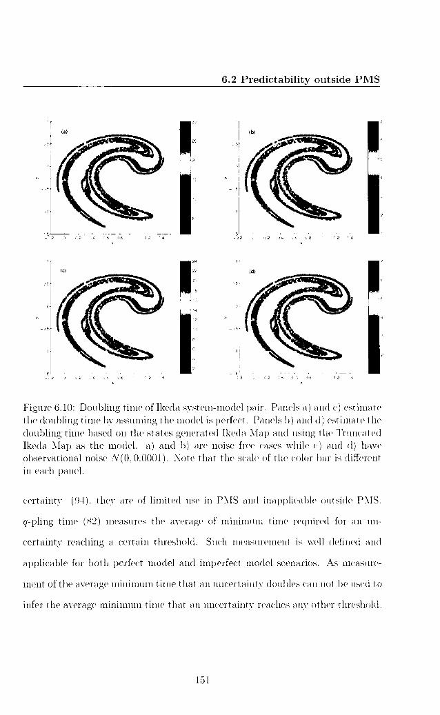
30
5
-02 0 02 r 8
05
-05
-14
0.5
0
0.5
0
-05
15 ' -02 0 02 04 0.6 08
X
1 1 .2 1 '4
05
-05
6.2 Predictability outside PMS
Figure 6.10: Doubling time of Ikeda system-model pair. Panels a) and c) estimate the doubling time by assuming the model is perfect. Panels b) and d) estimate the doubling time based on the states generated Ikeda Map and using the Truncated Ikeda Map as the model. a) and b) are noise free cases while c) and d) have observational noise N (0,0.0001). Note that the scale of the color bar is different in each panel.
certainty (94), they are of limited use in PMS and inapplicable outside PMS.
q-pling time (82) measures the average of minimum time required for an un-
certainty reaching a certain threshold. Such measurement is well defined and
applicable for both perfect model and imperfect model scenarios. As measure-
ment of the average minimum time that an uncertainty doubles can not be used to
infer the average minimum time that an uncertainty reaches any other threshold,
151

6.2 Predictability outside PMS
predictability being lost has to be defined, in advance, upon a certain threshold.
In this section we suggest another way to measure the predictability by compar-
ing the model forecast performance with climatology, we call it forecast based
measurement.
As the average forecast performance degenerates with forecast lead time, it
will, for sure, happens at certain lead time that the model forecast does not do
better than the climatology. We define predictability being lost when this hap-
pens, it indicates that the model forecast does no better than random drawn
from the historical observations. Such measurement can be applied to both per-
fect model and imperfect model scenarios and places no restriction on the initial
condition uncertainty. Comparing with the q-pling time, the predictability being
lost is better defined. Although the measurement itself places no restriction on
the initial uncertainties and the model, the model forecast performance depends
on how good the initial conditions and the model are. Similar to q-pling time,
the forecast based measurement measures the predictability given the initial con-
ditions and the model, of course, better initial conditions or better model will
have more predictability.
To evaluate the forecast performance, we use the Ignorance score (see sec-
tion 4.3.3). Given an initial condition ensemble and the model (does not have
to be perfect), the forecast ensemble at each lead can be produced by iterating
the initial condition through the model 1 . To calculate the imperical ignorance
score, a forecast ensemble is transformed into a forecast distribution by kernel
lwe are aware that one may use different forecast scheme, e.g. direct forecast and forecast with adjustment defined in section 6.1. In this section we treat the model and forecast scheme as the forecast model, i.e. forecasting using a deterministic model with random adjustment is treated to be a stochastic model
152
6.2 Predictability outside PMS
dressing (details of kernel dressing can be found in section 4.3.2). To simplify the
comparison between model forecast and climatology, the forecast distribution is
blended with climatology (details can be found in section 4.3.2). After blending
with climatology, we expect the forecast will do no worse than the climatology.
By looking at the Ignorance score relative to climatology, one can measure when
the predictability is lost. As the lead time goes larger, one may expect the relative
Ignorance go to zero asymptotically. When the model is perfect, given the sample
climatology based finite number of historical observations, we expect the relative
ignorance goes to the values that relevant to proportion between the size of the
ensemble and the size of the historical observations as the ensemble members will
eventually become random draws from the invariant measure of the model. When
the model is imperfect, we expect the relative ignorance goes to 0 eventually as
the invariant measure of the model is different from that of the system.
We suggest using the forecast based measurement to measure the predictabil-
ity as outside PMS the predictability should depend on not only the system and
model but also the way initial condition ensemble is constructed and the size of
ensemble. Figure 6.11 shows the ignorance score (relative to climatology) as a
function of forecast lead time in the Ikeda system-model pair experiment, fore-
cast based on two different initial condition ensembles with two different sizes are
plotted separately. In all cases, the relative ignorance converges to 0 after certain
lead time which indicates after that lead time the information in the initial condi-
tions is lost. Using the same initial condition ensemble but with larger ensemble
size provides more predictability and delay the convergence. As the results shown
in section 5.5.2, the initial condition ensemble formed by LSGDc produces better
estimate of the current states than the Inverse Noise ensemble, the information
153
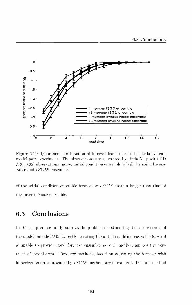
12 14 16 10 2 4 6 8 lead time
4 member ISGD ensemble 16 member ISGD ensemble 4 member Inverse Noise ensemble 16 member Inverse Noise ensemble
nora
nce r
elativ
e to c
limato
logy
0
- 0.5
- 1
-1.5
- 2
-2.5
- 3 -
- 3.5
- 40
6.3 Conclusions
Figure 6.11: Ignorance as a function of forecast lead time in the Ikeda system-model pair experiment. The observations are generated by Ikeda Map with IID N(0, 0.05) observational noise, initial condition ensemble is built by using Inverse Noise and ISGLY ensemble.
of the initial condition ensemble formed by ISGDc sustain longer than that of
the Inverse Noise ensemble.
6.3 Conclusions
In this chapter, we firstly address the problem of estimating the future states of
the model outside PMS. Directly iterating the initial condition ensemble forward
is unable to provide good forecast ensemble as such method ignores the exis-
tence of model error. Two new methods, based on adjusting the forecast with
imperfection error provided by ISGDC method, are introduced. The first method
154
6.3 Conclusions
adjust the forecast by adding random draws of the imperfection error onto the
forecast. The other method selects the imperfection error using analogue models.
Applying these methods to the Ikeda system-model pair, we demonstrate that
forecast with random adjustment does not provide significantly better estimates
than direct forecast as it discards the geometrical information of the imperfection
error. Forecast with analogue adjustment is shown to outperforms both direct
forecast and forecast with random adjustment.
Secondly we address the question of how to interpret predictability outside
PMS. Traditional ways of evaluating the predictability, Lyapunov exponents and
doubling time are discussed. Lyapunov exponents measure the predictability
through globally average error growth rates in the limits of large time and small
uncertainty, they are of limited use in PMS and inapplicable outside PMS. q-
pling time (82), which measures the average of minimum time required for an
uncertainty reaching a certain threshold, is applicable for both perfect model and
imperfect model scenarios. A certain threshold is, however, required in advance in
order to define when the predictability is lost. We suggest using the probabilistic
forecast skill to interpret the predictability. In that case, the predictability being
lost is well defined. In the IPMS, such forecast skill not only depends on the
system, and model, and observation method but also depends on the way that
initial conditions are formed and forecasts are determined from the ensemble.
155

Chapter 7
Conclusions
In this thesis, we addressed several nonlinear estimation problems by combining
statistical methods with dynamical insight.
Methods based on Indistinguishable States theory are introduced to estimate
the current state of the model in the PMS. By enhancing the balance between
the information contained in the dynamic equation and the information in the
observations, the IS method produces a good ensemble estimates of the current
state. Our methods are applied in Ikeda Map and Lorenz96 flow, and shown to
outperform the variational method, Four-dimensional Variational Assimilation,
and the sequential method, Ensemble Kalman Filter.
To estimate the model parameter, we introduced two new approaches, Fore-
cast Based estimates and Dynamical Coherent estimates. Forecast Based esti-
mates method estimate the parameter values based on the probabilistic forecast-
ing at a given lead time. Dynamical Coherent estimates method focuses on the
geometric properties of trajectories and the property of the pseudo-orbits pro-
vided by the ISGD method. Both methods are tested on a variety of nonlinear
models, the true parameter values are well identified.
Outside PMS, no model trajectories are consistent with infinite observations,
156
there are model pseudo-orbits that are consistent with the observations and their
corresponding imperfection error reflects the model error. we find applying the
ISGD method with a certain stopping criteria can produce such relevant pseudo-
orbits. Our methods are applied in Ikeda Map and Lorenz96 flow, and shown
to outperform the Weak Constrain Four-dimensional Variational Assimilation
method.
Given the fact that the model is imperfect, to estimate the future states
requires accounting the model inadequacy. We demonstrate that using the im-
perfection error produced by ISCDc method to adjust the forecast can improve
the forecast performance. Forecast based measurement is suggested to measure
the predictability outside PMS.
Main new results
• Chapter 3
—A new ensemble filter approach within the context of indistinguishable
states (48) is introduced to address the nowcasting problem in the
perfect model scenario.
—For the first time, IS method is compared with 4DVAR method when
both applying to Ikeda Map and Lorenz96 system which demonstrates
our method outperforms the 4DVAR method in state estimation.
—For the first time, IS method is compared with Ensemble Kalman
Filter method when both applying to Ikeda Map and Lorenz96 system
which demonstrates our method outperforms the EnKF method in
state estimation.
157

—A new probabilistic evaluation method, &ball, is introduced to evaluate
the ensemble forecasts.
• Chapter 4
—A new parameter estimation approach based on probabilistic forecast
is introduced.
—Another new parameter estimation approach, which focuses on the
geometric properties of trajectories, is introduced.
— For the first time, IS method, as part of the second parameter estima-
tion approach, is successfully applied to partial observations.
• Chapter 5
—A new methodology, i.e. applying the IS method with stopping criteria,
is introduced to address the nowcasting problem in the imperfect model
scenario.
—For the first time, our methodology is compared with WC4DVAR
method when both applying to Ikeda Map and Lorenz96 system which
demonstrates our method outperforms the WC4DVAR method in terms
of nowcasting.
—For the first time, we demonstrate that applying WC4DVAR method
will face the problem of increasing density of local minimums.
—For the first time, IS method is applied to form ensemble of initial
condition in the Imperfect Model Scenario.
• Chapter 6
158

— For the first time, we use the imperfection error obtained by apply-
ing IS method to adjust the forecast outside perfect model scenario.
And by applying in the Ikeda system-model pair, we demonstrate that
our method improves the forecast performance from direct forecast
significantly.
— Forecast based measurement is suggested to measure the predictability
outside PMS.
159
Appendix A
Gradient Descent Algorithm
In this appendix, we review the details of applying Gradient Descent (GD) Al-
gorithm (48; 50) to find the minimum of the mismatch cost function 3/ given a
sequence of observations s_N+1, ..•, so.
The minimum of the mismatch cost function can be obtained by solving the
ordinary differential equation
du d = —V C (u) r (A.1)
where C(u) is the mismatch cost function. In practice, we initialise the min-
imisation with the observations, i.e. u° = s. After every iteration of the GD
algorithm, the pseudo-orbit u will be updated (for instance, one obtain ul after j
iterations). To iterate the algorithm, one need to differentiate the mismatch cost
160

function given by
ac 2 au N +1
— (ut+i — F(ut))dtF(ut) t = —N + 1
—(ut — F(ut--1)) + (ut+1 — F(ut))d-tF(ut) —N +1 <t <0
—(ut — F(ut-1)) t =0
where dtF(ut ) is the Jacobian of the model F at ut . We solve the ordinary
differential equation A.1 using the Euler approximation.
161

Appendix B
Experiments Details
The tables below define the standard experiments which are used throughout the
thesis.
System Ikeda Map Noise model N(0, 0.05)
Number of assimilation 1024 Number of bootstrap samples 512
ISGD no. of GD iterations 4096 GD iteration step 0.2
4DVAR Initial GD iteration step 0.2 GD stops when iteration step < 5 x 10⁻⁶
Table B.1: Details of Experiment A, note for 4DVAR method we shrink the iteration step by 2 when cost function not decrease.
162

System Lorenz96 Model I Dimension of the system 18
Noise model N(0, 0.5) Number of assimilation 1024
Number of bootstrap samples 512 ISGD no. of GD iterations 4096
GD iteration step 1 4DVAR Initial GD iteration step 1
GD stops when iteration step < 10 -6
Table B.2: Details of Experiment B, note for 4DVAR method we shrink the iteration step by 2 when cost function not decrease.
System Ikeda Map Noise model N(0,0.05)
number of nowcast made 2048
ISIS
assimilation window length 12 steps no. of GD iterations 4096 perturbation of the middle points by N(0, 0.025) number of the perturbations 4096 number of ensemble members 512
EnKF number of ensemble members 512
Table B.3: Details of Experiment C
System Lorenz96 Model I Dimension of the system 18
Noise model N(0, 0.5) number of nowcast made 2048
ISIS
assimilation window length 1.2 time units no. of GD iterations 4096 perturbation of the middle points by N(0, 0.25) number of the perturbations 4096 number of ensemble members 512
EnKF number of ensemble members 512
Table B.4: Details of Experiment D
163

System Ikeda 1Vlap Noise model U(-0.025,0.025)
ISIS
window length 12 steps no. of GD iterations 4096 perturbation of the middle points by U(-0.01, 0.01) number of the perturbations 1024 number of ensemble members 64
DCEn number of ensemble members 64
Table B.5: Details of Experiment E
System Ikeda Map Lorenz96 Model II Model Truncated Ikeda Model Lorenz96 Model I Noise model N(0,0.01) N(0,0.4) number of observations 2048 102.4 time unit sample std of model error 0.018 0.0057
Table B.6: Details of Experiment F
System Ikeda Map Model Truncated Ikeda Model
Noise model N(0, 0.05) Number of assimilation 1024
Number of bootstrap samples 512 ISGDc no. of GD iterations 75
GD iteration step 0.2 WC4DVAR Initial GD iteration step 0.2
GD stops when iteration step < 5 x 10 -6
Table B.7: Details of Experiment G, note for WC4DVAR method we shrink the iteration step by 2 when cost function not decrease.
164

System Lorenz96 Model II Model Lorenz96 Model I
Dimension of the system 18 x 5 Noise model N(0,0.1)
Number of assimilation 1024 Number of bootstrap samples 512
ISCDc no. of GD iterations 4096 GD iteration step 1
WC4DVAR Initial GD iteration step 1 GD stops when iteration step < 10-6
Table B.8: Details of Experiment H, note for WC4DVAR method we shrink the iteration step by 2 when cost function not decrease.
165

Bibliography
[1] J.L. Anderson, An ensemble adjustment Kalman filter for data assimilation,
Mon. Weather Rev., 129, 2884-2903, (2001). 37, 41, 43
[2] J.L. Anderson, A local least squares framework for ensemble filtering, Mon.
Weather Rev., 131, 634-642, (2003). 37
[3] L. Arnold, Random Dynamical Systems, Springer, Berlin, (1998). 146
[4] A.F. Bennett, L.M. Leslie, C.R. Hagelberg and P.E. Powers, Tropical cy-
clone prediction using a barotropic model initialized by a generalized inverse
method. Mon. Wea. Rev., 121, 1714-1729, (1993). 111
[5] A.F. Bennett, B.S. Chua and L.M. Leslie, Generalized inversion of a global
numerical weather prediction model. Meteor. Atmos. Phys., 60, 165-178,
(1996). 111
[6] M.L. Berliner, Likelihood and Bayesian Prediction for Chaotic Systems, J.
Am. Stat. Assoc. 86, 938-952 (1991).
[7] C.H. Bishop, B.J.Etherton and S.J.Majumdar. Adaptive sampling with the
Ensemble Transform Kalman Filter. Part I: Theoretical Aspects. Mon. Wea.
Rev. 129, 420C436, (2001). 41, 43
166

BIBLIOGRAPHY
[8] A. Bjorck, Numerical Methods for Least Squares Problems, SIAM, (1996)
65
[9] E. Borel, Probability and Certainty Walker, New York, (1963). 80
[10] C.L.Bremer and D.T.Kaplan, Markov chain Monte Carlo estimation of non-
linear dynamics from time series, Physica D 160 116-126 (2001).
[11] G.W. Brier, Verification of forecasts expressed in terms of probabilities.
Mon. Wea. Rev., 78, 1C3, (1950).
[12] J. Brocker and L.A. Smith, Scoring Probabilistic Forecasts: On the Impor-
tance of Being Proper, Weather and Forecasting 22(2), 382-388, (2007) 53,
73
[13] J. Brocker and L.A. Smith, From ensemble forecasts to predictive distribu-
tion functions, submitted to Tellus, (2007) 70, 71
[14] D. S. Broomhead and D. Lowe. Multivariable functional interpolation and
adaptive networks. J. Complex Systems, 1:417-452, (1987). 17
[15] M. Casdagli. Nonlinear prediction of chaotic time series. Physica D, 35:335-
356, (1989). 17
[16] M. Casdagli, S. Eubank, J. D. Farmer, and J. Gibson, State space recon-
struction in the presence of noise, Physica D, 51, 52 (1991);
[17] G. Casella and R.L. Berger, Statistical Inference, Wadsworth, Belmont,
California, (1990). 66
167
BIBLIOGRAPHY
[18] P. Courtier and 0. Talagrand, Variational assimilation of meteorological ob-
servations with the adjoint vorticity equation. II: Numerical results, Q.J.R.
Meteorol Soc., 113, 1311-1328, (1987). 32
[19] P. Courtier, J.N. Thepaut and A. Hollingsworth, A strategy for operational
implementation of 4DVAR, using an incremental approach, Q.J.R. Meteorol
Soc., 120, 1367-1387, (1994). 32
[20] M.C. Cuellar, Perspectives and Advances in Parameter Estimation of Non-
linear Models. PhD Thesis, London School of Economics, (2007). 66, 78,
82
[21] M.E.Davies, Noise reduction by gradient descent, Int. J. Bifurcation Chaos
3, 113-118, (1992).
[22] J.-P. Eckmann, D. Ruelle, Rev. Mod. Phys. 57 617, (1985). 146
[23] G. Evensen, Sequential data assimilation with a nonlinear quasi-geostrophic
model using Monte Carlo methods to forecast error statistics, J. Geophys.
Res., 99, 10,143-10,162, (1994). 41
[24] G. Evensen, Sequential data assimilation with a nonlinear quasi-geostrophic
model using Monte Carlo methods to forecast error statistics, J. Geophys.
Res., 127, 2128-2142, (1994).
[25] J.P. Eckmann and D. Ruelle. Ergodic theory of chaos. Rev. Mod. Phys.,
45:617-656, 1985. 148
[26] J.D. Farmer and J.J. Sidorowich. Optimal shadowing and noise reduction.
Physica D, 47:373-392, (1991). 79
168

BIBLIOGRAPHY
[27] C. F. Gauss, Translated by G. W. Stewart. Theory of the Combination of
Observations Least Subject to Errors: Part One, Part Two, Supplement.
Philadelphia: Society for Industrial and Applied Mathematics, (1995). 65
[28] P. Gauthier, Chaos and quadri-dimensional data assimilation, A study
based on the Lorenz model. Telles 44A, 2-17, (1992).
[29] P. Gauthier, P. Courtier and P. Moll, Assimilation of simulated lidar data
with a Kalman filter, Mon. Weather Rev., 121, 1803-20, (1993). 40
[30] M. Ghil and P. IVIalanotte-Rizzoli, Data assimilation in meteorology and
oceanography, Adv. Geophys. 33, 141-266, (1991). 40
[31] I. Gilmour, Nonlinear model evaluation; t-shadowing, probabilistic predic-
tion and weather forecasting, Ph.D. thesis, University of Oxford, (1998).
79
[32] P. Grassberger, T. Schreiber, and C. Schaffrath, Non—linear time sequence
analysis, Int. J. Bif. and Chaos 1, 521 (1991).
[33] C. Grebogi, S.M. Hammel, J.A. Yorke, and T. Sauer. Shadowing of physical
trajectories in chaotic dynamics: containment and refinement. Phys. Rev.
Letts., 65(13):1527-1530, (1990). 79
[34] J. Guckenheimer, J. Moser and S. Newhouse, Dynamical Systems, LIME
Lectures, Birkhauser, 289pp., (1980).
[35] J. Guckenheimer and P. Holmes, Nonlinear Oscillations, Dynamical Sys-
tems, and Bifurcations of Vector Fields, Springer, New York, (1983). 7
169

BIBLIOGRAPHY
[36] T.M. Hamill, Iterpretation of Rank Histograms for Verifying Ensemble
Forecasts. Monthly Weather Review: Vol. 129, No. 3, 9-30, (2001)
[37] T.M. Hamill, Ensemble-based atmospheric data assimilation, Chapter 6 of
Predictability of Weather and Climate, Cambridge Press, 124-156, (2006).
41, 42, 43, 44, 73
[38] J.A.Hansen, Adaptive observations in spatialy-extended nonlinear dynam-
ical systems, Ph.D. thesis, University of Oxford, (1998).
[39] J.A. Hansen, L.A. Smith, Probabilistic noise reduction. Tellus series A, 53
(5), 585-598 (2001). 48
[40] M. Henon, A two-dimensional mapping with a strange attractor, Commun.
Math. Phy, s. 50 69-77 (1976). 10
[41] P.L. Houtekamer and H.L. Mitchell. Data assimilation using an ensemble
Kalman filter technique. Mon. Weather Rev., 126, 796-811, (1998). 41, 42
[42] P.L. Houtekamer and H.L. Mitchell. Reply to comment on "Data assimila-
tion using an ensemble Kalman filter technique." Mon. Weather Rev., 127,
1378-9, (1999). 41, 42
[43] P.L. Houtekamer and H.L. Mitchell. A sequential ensemble Kalman filter
for atmospheric data assimilation. Mon. Weather Rev., 129, 123-37, (2001).
41, 42
[44] G.E. Hutchinson, Circular casual systems in ecology, Annals of the New
York Academy of Sciences, 50, 221-246, (1948). 8
170

BIBLIOGRAPHY
[45] K. Ikeda, Multiple valued stationarity state and its instability of the trans-
mitted light by a ring cavity system, Optical Communications, 30 257-261
(1979). 11
[46] L. Jaeger and H. Kantz, Unbiased reconstruction of the dynamics underly-
ing a noisy chaotic time series, Chaos 6, 440 (1996).
[47] A.H. Jazwinski, Stochastic Processes and Filtering Theory. Academic Press,
(1970). 40
[48] K. Judd and L.A. Smith, Indistinguishable States I: The Perfect Model
Scenario, Physica D 151: 125-141, (2001). 2, 19, 22, 25, 27, 28, 34, 65, 98,
157, 160
[49] K. Judd, Chaotic-time-series reconstruction by the Bayesian paradigm:
Right results by wrong methods, Physics Review Letters, 67,
026212,(2003).
[50] K. Judd and L.A. Smith, Indistinguishable States II: The Imperfect Model
Scenario, Physica D 196: 224-242, (2004). 3, 11, 93, 94, 95, 96, 98, 100,
108, 110, 126, 129, 160
[51] K. Judd and L.A. Smith and A. Weisheimer, Gradient free descent: shad-
owing and state estimation with limited derivative information, Physica D,
190, 153-166 (2004). 90
[52] K. Judd, Forecasting with imperfect models, dynamically constrained in-
verse problems, and gradient descent algorithms, Physica D, 237, 216-232,
(2008). 34, 114
171
BIBLIOGRAPHY
[53] K. Judd, C.A. Reynolds, T.E. Rosmond and L.A. Smith, The Geometry of
Model error, Journal of Atmospheric Science, 65 (6), 1749-1772, 2008 29,
56, 62
[54] R. E. Kalman, A New Approach to Linear Filtering and Prediction Prob-
lems. Trans AMSE Ser D J Basic Eng, 82, 35-45, (1960). 37
[55] H. Kautz and L. Jaeger, Homoclinic tangencies and non-normal Jacobians
- effects of noise in non-hyperbolic systems, Physica D 105, 79-96 (1997).
[56] T. Kariya, H. Kurata, Generalized Least Squares, Wiley, (2004). 65
[57] J.L. Kelly, Jr, A New Interpretation of Information Rate, Bell System Tech-
nical Journal, 35, 917-926, (1956) 74
[58] E.J. Kostelich and J.A. Yorke, Noise Reduction in Dynamical Systems,
Phys Rev A 38, 1649, (1988). 79
[59] E.J. Kostelich, Problems in estimating dynamics from data, Physica D 58,
138 (1992).
[60] S.A. Levin and R.M. May, A note on difference-delay equations, Theoretical
Population Biology, 9, 178-187, (1976). 8
[61] E.N. Lorenz, Deterministic nonperiodic flow. J. Atmos. Sci., 20:130-141,
(1963). 10, 34
[62] E.N. Lorenz. A study of the predictability of a 28-variable atmospheric
model. Tellus, 17:321-333, (1965). 146, 147, 148
172

BIBLIOGRAPHY
[63] E.N. Lorenz, Predictability A problem partly solved, in: ECMWF Seminar
Proceedings on Predictability, Reading, United Kingdom, ECMWF, (1995).
12, 13, 96
[64] P.E. McSharry and L.A. Smith, Better nonlinear models from noisy data:
Attractors with maximum likelihood, Phys. Rev. Lett 83, (21): 4285-4288,
(1999). 3, 63, 65, 66, 86, 87, 103, 185
[65] R.N. Miller, M. Ghil and F. Gauthiez, Advanced data assimilation in
strongly nonlinear dynamical systems. J.Atmos.Sci. 51, 1037-1056, (1994).
32, 33
[66] W. D.Moore and E. A.Spiegel, A thermally excited nonlinear oscillator.
The Astrophysical Journal. Volume 143, pp. 871-887, (1966). 12
[67] D. Orrell, A shadow of a Doubt: Model Error, Uncertainty, and shadowing
in Nonlinear Dynamical Systems. PhD Thesis, University of Oxford, (1999).
13
[68] V.I. Oseledec, Transactions of the Moscow Mathematical Society 19 197,
(1968). 146
[69] E. Ott, Chaos in Dynamical Systems, Cambridge University Press, (1993).
9
[70] F. Paparella, A. Provenzale, L.Smith, C.Taricco, R.Vio, Local Random ana-
logue prediction of nonlinear processes, Phys. Lett. A 235 233-240, (1997).
16, 132
173

BIBLIOGRAPHY
[71] C. Pires, R. Vautard, and 0. Talagrand, On extending the limits of vari-
ational assimilation in nonlinear chaotic systems. Tellus, 48A, 96-121,
(1996). 32, 33, 34, 36
[72] V.F. Pisarenko and D. Sornette, Statistical methods of parameter estima-
tion for deterministically chaotic time series, Phys Rev E, 69 (2004).
[73] W. H. Press, B. Flannery, S. Teukolsky, and W. Vetterling, Numerical
Recipes in C (CUP, Cambridge, 1992).
[74] D. Ridout and K. Judd, Convergence properties of gradient descent noise
reduction. Physica D 165 27-48, (2001).
[75] M.S. Roulston and L.A. Smith, Evaluating probabilistic forecasts using
information theory, Monthly Weather Review, 130, 1653-1660, (2002) 70,
73 1
[76] Y. Sasaki, Some basic formalisms on numerical variational analysis. Mon.
Wea. Rev., 98, 875-883, (1970). 111
[77] T. Sauer, J.A. Yorke, M. Casdagli, Embedology, J. Stat. Phys. 65, 579,
(1991). 79
[78] D.S. Sivia, Data analysis - a Bayesian tutorial, Clarendon Press, Oxford
University Press, (1997).
[79] L. A. Smith. Identification and prediction of low-dimensional dynamics.
Physica D, 58:50-76, (1992). 15, 17, 131
[80] L. A. Smith. Accountability and error in forecasts. In Proceedings of the
1995 ECMWF Predictability Seminar, (1996). 45, 46, 92
174

BIBLIOGRAPHY
[81] L.A. Smith. The Maintenance of Uncertainty, Proc International School of
Physics "Enrico Fermi", Course CXXXIII, pg 177-246, Societa Italiana di
Fisica, Bologna, Italy (1997). 15, 147, 148, 149
[82] L. A. Smith, C. Ziehman, and K. Raedrich. Uncertainty in dymanamics and
predictability in chaotic systems. Q. J. R. Meteorol. Soc., 125:2855C2886,
(1999). 146, 148, 149, 151, 155
[83] L.A. Smith, Disentangling Uncertainty and Error: On the Predictability
of Nonlinear Systenis. Nonlinear Dynamics and Statistics, A.I.Mees, Ed.,
Birkhauser, 31-64 (2000). 13, 79
[84] L.A. Smith and M.S. Roulston, Evaluating Probabilistic Forecasts Using
Information Theory. Monthly Weather Review 130, no. 6, pp. 1653-1660,
(2001).
[85] L.A. Smith, M.C. Cuellar, H. Du, and K. Judd, Identifying dynamically
coherent behaviours: A geometrical approach to parameter estimation in
nonlinear models, Physics Letter A, under review (2009). 78
[86] H. Sorenson, Kalman Filtering: Theory and Application. IEEE Press,
(1985). 37
[87] D.A.Stainforth, et al. Uncertainty in predictions of the climate response to
rising levels of greenhouse gases, Nature, 433, 403C406, (2005). 89
[88] D.J. Stensrud and J.1AT. Bao, Behaviors of variational and nudging assim-
ilation techniques with a chaotic low-order model. Mon. Wea. Rev. 120,
3016-3028, (1992).
175
BIBLIOGRAPHY
[89] F. Takens. Detecting strange attractors in fluid turbulence. In D. Rand and
L.-S. Young, editors, Dynamical Systems and Turbulence, pages 366-381,
Berlin, Springer-Verlag, (1981). 15
[90] 0. Talagrand and P. Courtier, Variational assimilation of meteorological
observations with the adjoint vorticity equation. I: Theory, Q.J.R. Nleteorol
Soc., 113, 1311-1328, (1987). 32, 111
[91] J. Timmer, Modeling noisy time series: physiological tremor, Int. J. Bif.
Chaos 8, 1505C1516 (1998).
[92] J.S. Whitaker and T.M. Hamill, Ensemble data assimilation without per-
turbed observations. Mon. Weather Rev., 130, 1913-24, (2002). 43
[93] D.S. Wilks, Comparison of ensemble-MOS methods in the Lorenz'96 set-
ting. Meteorological Applications, 13, (2006). 71
[94] C. Ziehmann, L.A. Smith and J. Kurths, Localized Lyapunov Exponents
and the Prediction of Predictability Phys. Lett. A, 271 (4): 237-251, (2000).
148, 151
176

Nomenclature
Roman Symbols
71 observational noise or measurement error
5 implied noise
F covariance matrix of the observational noise
co imperfection error
C forecast adjustment
A attractor or invariant measure
11-11(x) the set of indistinguishable states of x
M model space
0 observation space
S state space
I.(x) unconditional probability density function of x
p(•) probability density function of the observation noise
177

BIBLIOGRAPHY
a model parameter
B covariance matrix of xb
e mismatch error
ui component of a pseudo-orbit
x model state
xa the posteriori estimate of system state
xb first guess or background state of the model
y pseudo-orbit obtained by ISGD method
z reference trajectory
a system parameter
system state
F system dynamics
dimension of the system parameter space
rrz dimension of the system space
F model dynamics
h(•) observation operator
Kt Kalman gain
dimension of the model parameter space
178

BIBLIOGRAPHY
m dimension of the model space
n number of observations
N"nd number of candidate trajectories
Neils number of ensemble members
pa analysis-error covariance
Pb background-error covariance
Q the density function measures the indistinguishability
Y verification
179
List of Figures
2.1 The bifurcation diagram of logistic map 9
2.2 The attractor of Henon Map 10
2.3 The attractor of Ikeda Map 11
2.4 The attractor of Moore-Spiegel system for T = 36 and R = 100. 13
3.1 Following Judd and Smith (2001), Suppose xt is the true state of
the system and y t some other state where x t and yt E R2 . The
circles centred on xt and yt represent the bounded measurement
error. When an observation falls in the overlap of the two circles
(e.g., at a), then the states xt and y t are indistinguishable given
this single observation. If the observation falls in the region about
xt , but outside the overlap region (e.g., at 13), then on the basis of
this observation one can reject y t being the true state, i.e., x t and
yt are distinguishable given the observation. 22
3.2 Schematic flowchart of the IS nowcasting algorithm
180
LIST OF FIGURES
3.3 Example of perfect ensemble for the Ikeda Map when only one
observation is considered. The observational noise is uniformly
bounded. In panel a, the black dots indicate samples from the
Ikeda Map attractor, the blue circle denotes the bounded noise
region where the single observation is the centre of the circle. Panel
b is the zoom-in plot of the bounded noise region. The red cross
denotes the true state of the system 46
3.4 Following Figure 3.3, examples of perfect ensemble are shown for
the Ikeda Map when more than one observation is considered. The
perfect ensemble of different number observations are considered
are plotted separately. Two observations are considered in panel
(a), 4 in panel (b), 6 in panel (c) and 8 in panel (d). In all the
panels, the green dots are indicates the members of perfect ensemble. 47
3.5 Ensemble results from both EnKF and ISIS for the Ikeda Map (Ex-
periment C). The true state of the system is centred in the picture
located by the cross; the square is the corresponding observation;
the background dots indicate samples from the Ikeda Map attrac-
tor. The EnKF ensemble is depicted by 512 purple dots. Since the
EnKF ensemble members are equally weighted, the same colour is
given. The ISIS ensemble is depicted by 512 coloured dots. The
colouring indicates their relative likelihood weights. Each panel is
an example of one nowcast.
181
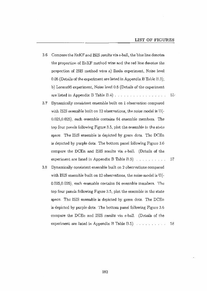
LIST OF FIGURES
3.6 Compare the EnKF and ISIS results via &ball, the blue line denotes
the proportion of EnKF method wins and the red line denotes the
proportion of ISIS method wins a) Ikeda experiment, Noise level
0.05 (Details of the experiment are listed in Appendix B Table B.3);
b) Lorenz96 experiment, Noise level 0.5 (Details of the experiment
are listed in Appendix B Table B.4) 55.
3.7 Dynamically consistent ensemble built on 1 observation compared
with ISIS ensemble built on 12 observations, the noise model is U(-
0.025,0.025), each ensemble contains 64 ensemble members. The
top four panels following Figure 3.5, plot the ensemble in the state
space. The ISIS ensemble is depicted by green dots. The DCEn
is depicted by purple dots. The bottom panel following Figure 3.6
compare the DCEn and ISIS results via e-ball. (Details of the
experiment are listed in Appendix B Table B.5) 57
3.8 Dynamically consistent ensemble built on 2 observations compared
with ISIS ensemble built on 12 observations, the noise model is U(-
0.025,0.025), each ensemble contains 64 ensemble members. The
top four panels following Figure 3.5, plot the ensemble in the state
space. The ISIS ensemble is depicted by green dots. The DCEn
is depicted by purple dots. The bottom panel following Figure 3.6
compare the DCEn and ISIS results via c-ball. (Details of the
experiment are listed in Appendix B Table B.5)
182

LIST OF FIGURES
3.9 Dynamically consistent ensemble built on 6 observations compared
with ISIS ensemble built on 12 observations, the noise model is 15(-
0.025,0.025), each ensemble contains 64 ensemble members. The
top four panels following Figure 3.5, plot the ensemble in the state
space. The ISIS ensemble is depicted by green dots. The DCEn
is depicted by purple dots. The bottom panel following Figure 3.6
compare the DCEn and ISIS results via e-ball. (Details of the
experiment are listed in Appendix B Table B.5) 59
3.10 Dynamically consistent ensemble built on 12 observations com-
pared with ISIS ensemble built on 12 observations, the noise model
is U(-0.025,0.025), each ensemble contains 64 ensemble members.
The top four panels following Figure 3.5, plot the ensemble in the
state space. The ISIS ensemble is depicted by green dots. The
DCEn is depicted by purple dots. The bottom panel following
Figure 3.6 compare the DCEn and ISIS results via 6-ball. (Details
of the experiment are listed in Appendix B Table B.5) 60
4.1 Parameter estimation using LS cost functions for different noise
level, the black shading reflects the 95% limits and the red solid
line is the mean, they are calculated from 1000 realizations and
each cost function is calculated based on the observations with
length 100, the blue flat line indicates the true parameter value
(a) Logistic Map for a = 1.85 (b) Ikeda Map for u = 0.83 67
183

LIST OF FIGURES
4.2 LS cost function in the parameter space, (a) Moore-Spiegel Flow
with true parameter value R=100 (vertical line), Noise level=0.05;
(b) Henon Map with true parameter values a=1.4 and b=0.3 (white
plus), Noise level=0.05. In each case, LS cost function is calculated
based on 2048 observations. 68
4.3 Schematic flowchart of obtaining forecast based cost function for
parameter estimation 69
4.4 Parameter estimation based on ignorance score, 64-member initial
condition ensemble is formed by inverse noise, the kernel parameter
and blending parameter is trained based on 2048 forecasts and
the empirical ignorance score is calculated base on another 2048
forecasts, the ignorance relative to climatology, i.e. 0 represents
climatology, is plotted in the parameter space (a) Logistic Map
with true parameter value a=1.85, results of different noise levels
are plotted separately; (b) Henon Map with true parameter values
a=1.4 and b=0.3, Noise level=0.05 76
4.5 Following Figure 4.4a, Parameter estimation using ignorance for
Logistic Map with alpha=1.85 (a) Lead time 1 forecast Ignorance(b)
Lead time 2 forecast Ignorance (c) Lead time 4 forecast Ignorance
(d) Lead time 6 forecast Ignorance. 77
4.6 Follow Figure 4.5, Parameter estimation using forecast Ignorance
Score for logistic map with a=1.85, initial condition ensemble formed
by dynamical consistent ensemble, a) based on lead time 1 forecast
b) based on lead time 4 forecast. Note scale change on y axis from
Figure 4.4a and 4.5. 78
184

LIST OF FIGURES
4.7 The standard deviation of implied noise as a function of number of
ISGD iterations for Ikeda Map with true parameter value u=0.83,
the black horizontal line denotes the noise level. The statistics for
tests using different parameter values are plotted separately. . . . 83
4.8 Parameter estimations for Ikeda Map with u=0.83 and noise level ,-----0.02;
Moore-Spiegel System with R=100 and noise level=0.05, the re-
sults are calculated base on 1024 observations, (a) and (d) The
median (solid), 90% (dashed) and 99% (dash-dot) shadowing iso-
pleths; (b) and (e) standard deviation of the mismatch; (c) and (f)
standard deviation of the implied noise, the horizontal line denotes
the real noise model. The vertical line represents the location of
the unknown true parameter. 85
4.9 Information from a pseudo-orbit determined via gradient descent
applied to a 1024 observations of the Henon map with a noise level
of 0.05. (a) standard deviation of the mismatch, (b) the implied
noise level, (c) a cost function based on the model's invariant mea-
sure (after Fig.4(b) of ref (64)), (d) median of shadowing time
distribution 87
4.10 Shadowing time isopleths as in Figure 4.8 for 8-D Lorenz96 with
parameter F=10 given only partial observations, a) the 8th com-
ponent of the state vector is not observed; b) none of the 2nd, 5th
or 8th variables are observed only the other five components; c)
only 2nd, 5th or 8th variables are observed; d) all the components
of the state vector are observed. In this experiment the noise level
is 0 2 88
185
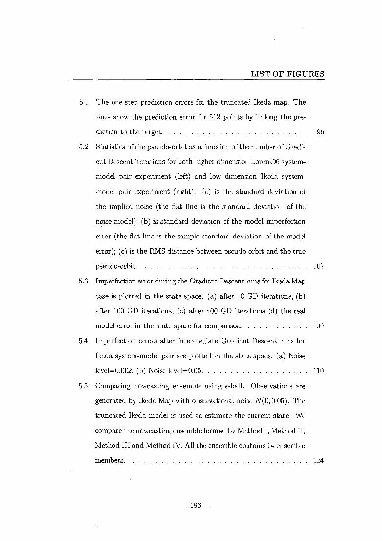
LIST OF FIGURES
5.1 The one-step prediction errors for the truncated Ikeda map. The
lines show the prediction error for 512 points by linking the pre-
diction to the target. 96
5.2 Statistics of the pseudo-orbit as a function of the number of Gradi-
ent Descent iterations for both higher dimension Lorenz96 system-
model pair experiment (left) and low dimension Ikeda system-
model pair experiment (right). (a) is the standard deviation of
the implied noise (the flat line is the standard deviation of the
noise model); (b) is standard deviation of the model imperfection
error (the flat line is the sample standard deviation of the model
error); (c) is the RMS distance between pseudo-orbit and the true
pseudo-orbit. 107
5.3 Imperfection error during the Gradient Descent runs for Ikeda Map
case is plotted in the state space. (a) after 10 GD iterations, (b)
after 100 GD iterations, (c) after 400 GD iterations (d) the real
model error in the state space for comparison. 109
5.4 Imperfection errors after intermediate Gradient Descent runs for
Ikeda system-model pair are plotted in the state space. (a) Noise
level=0.002, (b) Noise level=0.05 110
5.5 Comparing nowcasting ensemble using &ball. Observations are
generated by Ikeda Map with observational noise N(0, 0.05). The
truncated Ikeda model is used to estimate the current state. We
compare the nowcasting ensemble formed by Method I, Method II,
Method III and Method IV. All the ensemble contains 64 ensemble
members. 124
186
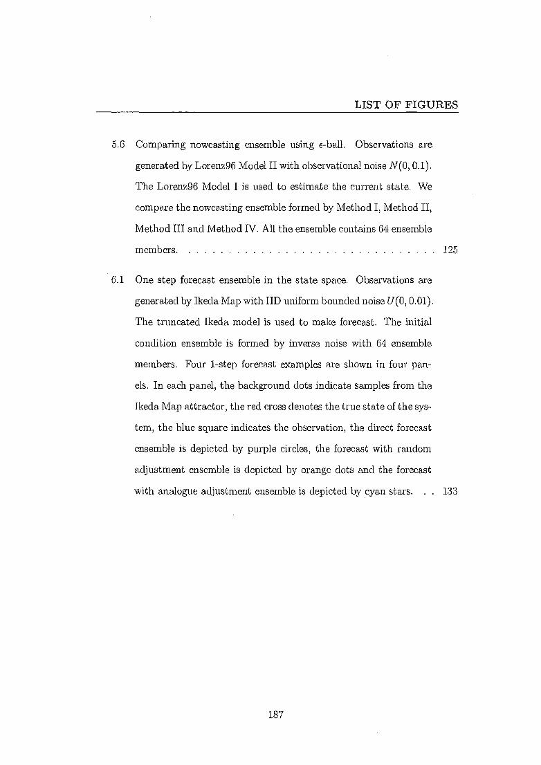
LIST OF FIGURES
5.6 Comparing nowcasting ensemble using 6-ball. Observations are
generated by Lorenz96 Model II with observational noise N(0, 0.1).
The Lorenz96 Model I is used to estimate the current state. We
compare the nowcasting ensemble formed by Method I, Method II,
Method III and Method IV. All the ensemble contains 64 ensemble
members. 125
6.1 One step forecast ensemble in the state space. Observations are
generated by Ikeda Map with IID uniform bounded noise U(0, 0.01).
The truncated Ikeda model is used to make forecast. The initial
condition ensemble is formed by inverse noise with 64 ensemble
members. Four 1-step forecast examples are shown in four pan-
els. In each panel, the background dots indicate samples from the
Ikeda Map attractor, the red cross denotes the true state of the sys-
tem, the blue square indicates the observation, the direct forecast
ensemble is depicted by purple circles, the forecast with random
adjustment ensemble is depicted by orange dots and the forecast
with analogue adjustment ensemble is depicted by cyan stars. . . 133
187

LIST OF FIGURES
6.2 Following Figure 6.1 experiment setting, compare forecast ensem-
ble using 6-ball. Direct forecasts are compared with forecasts with
random adjustment (left) and forecasts with analogue adjustment
(right). The initial condition ensemble is formed by inverse noise
with 64 ensemble members. For each forecast method, 2048 fore-
casts are made. Each row shows the comparison for different lead
time. First row denotes lead time 1, second lead time 2, third lead
time 4, forth lead time 8 and fifth lead time 16. 135
6.3 Following Figure 6.1 one step forecast ensemble in the state space.
The initial condition ensemble is formed by dynamical consistent
ensemble with 64 ensemble members. :136
6.4 Comparing forecast ensemble using 6-ball. Observations are gen-
erated by Ikeda Map with IID uniform bounded noise U(0, 0.01).
The truncated Ikeda model is used to make forecast. The initial
condition ensemble is formed by dynamical consistent ensemble
with 64 ensemble members. Each row of pictures shows the com-
parison for different lead time. First row denotes lead time 1,
second lead time 2, third lead time 4, forth lead time 8 and fifth
lead time 16. 137
188

LIST OF FIGURES
6.5 Following Figure 6.1 experiment setting, Ignorance score of three
forecasting methods relative to climatology is plotted vs lead time.
The error bars are 90% bootstrap re-sampling bars. In panel (a),
the initial condition ensemble is formed by inverse noise with 64
ensemble members. In panel (b), the initial condition ensemble is
formed by dynamical consistent ensemble with 64 ensemble mem-
bers. Panel (c) is the combination of panel (a) and (b). Ignorance
is calculated based upon 2048 forecasts. 139
6.6 Following Figure 6.1, six 1-step forecast examples are plotted in
the state space. Here the adjustment is obtained from imperfection
error instead of model error 142
6.7 Following Figure 6.2, comparing three forecast ensemble results
using c-ball. Here the adjustment is obtained from imperfection
error instead of model error 143
6.8 Following Figure 6.5a, Ignorance score of three forecasting methods
relative to climatology is plotted vs lead time. Forecast adjustment
is obtained from imperfection error 144
6.9 Ignorance score of forecast with adjustment where the adjustment
is generated from the observations with different noise level. The
initial condition ensemble is formed by inverse noise with fixed
noise level U(0, 0.01) so that the observations with different noise
level only affect the imperfection error. The error bars are 90%
bootstrapped error bars. In panel a, the forecast is made by ran-
dom adjustment; in panel b, the forecast is made by analogue
adjustment :145
189
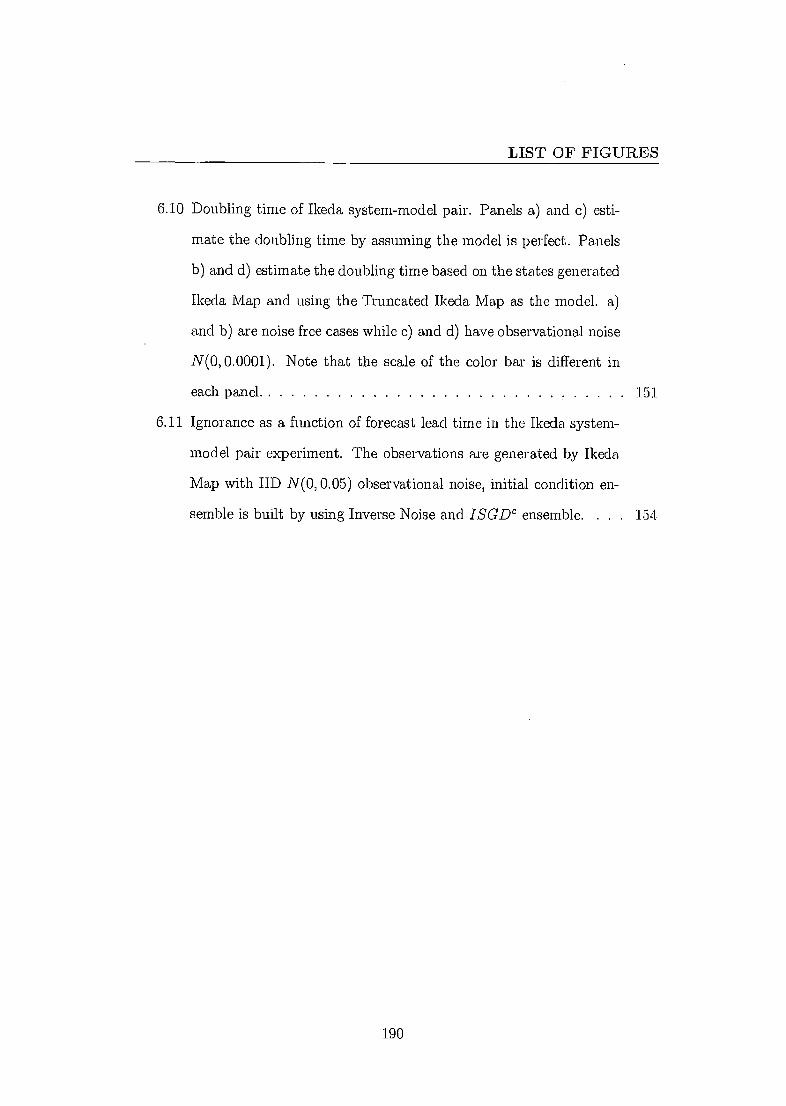
LIST OF FIGURES
6.10 Doubling time of Ikeda system-model pair. Panels a) and c) esti-
mate the doubling time by assuming the model is perfect. Panels
b) and d) estimate the doubling time based on the states generated
Ikeda Map and using the Truncated Ikeda Map as the model. a)
and b) are noise free cases while c) and d) have observational noise
N(0, 0.0001). Note that the scale of the color bar is different in
each panel. 151
6.11 Ignorance as a function of forecast lead time in the Ikeda system-
model pair experiment. The observations are generated by Ikeda
Map with IID N(0, 0.05) observational noise, initial condition en-
semble is built by using Inverse Noise and ISG.Dc ensemble. . . . 154
190