Ls Dyna Beams

8/9/2019 Ls Dyna Beams

http://slidepdf.com/reader/full/ls-dyna-beams 1/18

LS-DYNA Beam Elements: Default and User DefinedCross Section Integration

Author:

Len Schwer Schwer Engineering & Consulting Services, USA

Correspondence:

Len Schwer Schwer Engineering & Consulting Services

6122 Aaron CourtWindsor CA 95492-8651

USA

e-mail: [email protected]

Keywords:Beam, cross section, integration, user supplied integration,

*Section_Beam, *Integration_Beam, *Integration_Beam

4th

European LS-DYNA Users Conference Implicit / New Developments

H – I - 31



ABSTRACT

LS-DYNA provides several beam element formulations, see the keyword descriptionfor *Section_Beam in the User’s Manual. Several of these beam elementformulations support user supplied integration of the cross section, via the*Integration_Beam keyword. While most LS-DYNA users are familiar with the similar through-the-thickness integration algorithm for shell elements, which is made trivialby the rectangular cross section geometry assumed for shell elements, the numericalintegration of even simple beam element cross sections requires more effort, and aswill be demonstrated, more planning.

In this article, a detailed explanation of the beam element cross section integrationalgorithm is presented. Simple suggestions for calculating, and checking, user provided integration rules are illustrated through several examples. The examples

also provide suggestions for improving the LS-DYNA Standard Cross Section Types,available via the ICST parameter of the *Integration_Beam keyword.

ANALYTICAL INTEGRATION

To provide a basis for assessing the numerical integration algorithm, used in LS-DYNA, for beam element cross sections, we first establish the correspondinganalytical results. There are two cross section integrations that will be considered:axial force and bending moment; the former is relatively straight forward and isincluded only for completeness.

Axial Force

The axial force in a beam element is obtained by integrating the axial stress over thecross section,

( ), F dA y z dydz σ σ = = ∫ ∫ (1)

where ( ), y z σ σ = is the axial stress which typically varies over the cross sectional

area in the y z − plane.

Bending Moment

The moments, about the local y and z axes, in a beam element are obtained by

integrating the axial stress times the appropriate distance (moment arm) over thecross section,

( )

( )

,

,

y

z

M zdA y z zdydz

M ydA y z ydydz

σ σ

σ σ

= =

= =

∫ ∫ ∫ ∫

(2)

Implicit / New Developments 4th

European LS-DYNA Users Conference

H – I - 32



where local y and z axes are often the centrodial axes of the cross section, but

may be any convenient cross sectional axes. Recall that the centrodial axis can belocated relative to any axis via

c

zdA z

A= ∫

(3)

where c z provides the distance from the z axis to the centroid. Centroids lie along

planes of symmetry, if they exist in a cross section, as the above integral is zero for symmetric limits of the variable z , i.e. the cross section is symmetric with respect tothe y− plane.

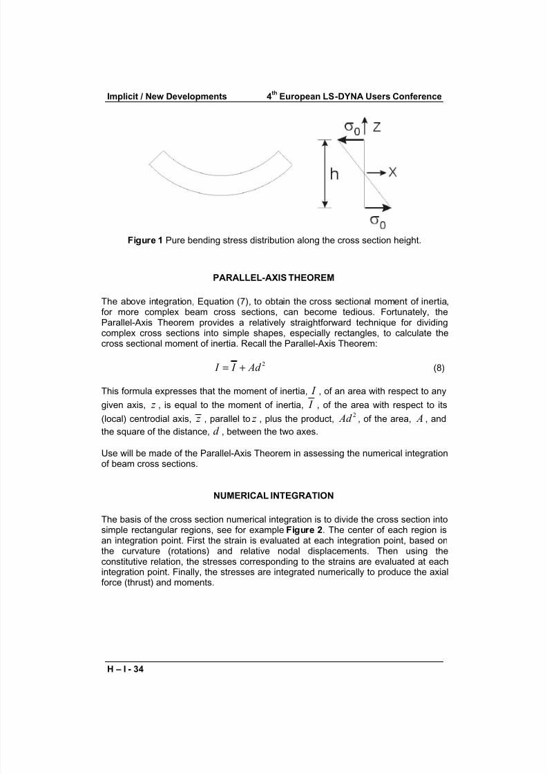
For the special case of pure bending about only one axis, say the y axis, with a

symmetric cross section, the axial stress may be written as

( ) 0

2 z z

hσ σ σ = = (4)

where0

σ is the maximum (outer fiber) stress and / 2 / 2h z h− < < where h is the

height of the cross section, see Figure 1, and for simplicity consider a rectangular

cross section of width b .

Substitution of the above linear stress distribution into the first of Equations (2) yields

( )/ 2 / 2 / 2

2

0

/ 2 / 2 / 2

3

00

2

2

12

b h h

y

A b h h

yy

b M zdA dy z zdz z dz

h

bh I

h c

σ σ σ

σ

σ

− − −

= = =

= =

∫ ∫ ∫ ∫ (5)

Inverting the above provides the familiar strength of materials result

0

Mc

I σ = (6)

where / 2c h= and yy

I is the cross sectional moment of inertia, and has the

following familiar form

/ 2 32 2

/ 212

h

yy

A h

bh I z dA b z dz

−

= = = ∫ ∫ (7)

when z is the centrodial axis.

4th


H – I - 33



Figure 1 Pure bending stress distribution along the cross section height.

PARALLEL-AXIS THEOREM

The above integration, Equation (7), to obtain the cross sectional moment of inertia,for more complex beam cross sections, can become tedious. Fortunately, theParallel-Axis Theorem provides a relatively straightforward technique for dividingcomplex cross sections into simple shapes, especially rectangles, to calculate thecross sectional moment of inertia. Recall the Parallel-Axis Theorem:

2 I I Ad = + (8)

This formula expresses that the moment of inertia, I , of an area with respect to any

given axis, z , is equal to the moment of inertia, I , of the area with respect to its(local) centrodial axis, z , parallel to z , plus the product,

2 Ad , of the area, A , and

the square of the distance, d , between the two axes.

Use will be made of the Parallel-Axis Theorem in assessing the numerical integrationof beam cross sections.

NUMERICAL INTEGRATION

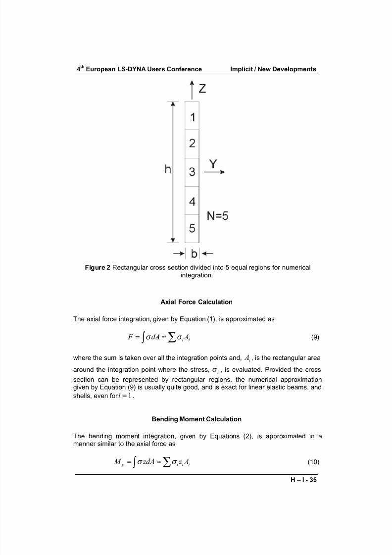
The basis of the cross section numerical integration is to divide the cross section intosimple rectangular regions, see for example Figure 2. The center of each region is

an integration point. First the strain is evaluated at each integration point, based onthe curvature (rotations) and relative nodal displacements. Then using theconstitutive relation, the stresses corresponding to the strains are evaluated at eachintegration point. Finally, the stresses are integrated numerically to produce the axialforce (thrust) and moments.



H – I - 34



Figure 2 Rectangular cross section divided into 5 equal regions for numericalintegration.

Axial Force Calculation

The axial force integration, given by Equation (1), is approximated as

i i F dA Aσ σ = ≈ ∑ ∫ (9)

where the sum is taken over all the integration points and,i

A , is the rectangular area

around the integration point where the stress, iσ , is evaluated. Provided the cross

section can be represented by rectangular regions, the numerical approximation

given by Equation (9) is usually quite good, and is exact for linear elastic beams, andshells, even for 1i = .

Bending Moment Calculation

The bending moment integration, given by Equations (2), is approximated in amanner similar to the axial force as

y i i i M zdA z Aσ σ = ≈ ∑ ∫ (10)

4th


H – I - 35



where the distancei

z is measured from the integration point to the y axis, about

which the moment is being calculated.

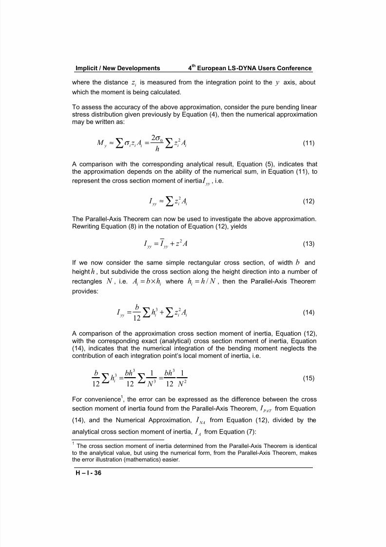
To assess the accuracy of the above approximation, consider the pure bending linearstress distribution given previously by Equation (4), then the numerical approximationmay be written as:

202

y i i i i i M z A z A

h

σ

σ ≈ =∑ ∑ (11)

A comparison with the corresponding analytical result, Equation (5), indicates thatthe approximation depends on the ability of the numerical sum, in Equation (11), to

represent the cross section moment of inertia yy

I , i.e.

2

yy i i I z A≈ ∑ (12)

The Parallel-Axis Theorem can now be used to investigate the above approximation.Rewriting Equation (8) in the notation of Equation (12), yields

2

yy yy I I z A= + (13)

If we now consider the same simple rectangular cross section, of width b and

height h , but subdivide the cross section along the height direction into a number of

rectangles N , i.e. i i A b h= × where /

ih h N = , then the Parallel-Axis Theorem

provides:

3 2

12 yy i i i

b I h z A= +∑ ∑ (14)

A comparison of the approximation cross section moment of inertia, Equation (12),with the corresponding exact (analytical) cross section moment of inertia, Equation(14), indicates that the numerical integration of the bending moment neglects thecontribution of each integration point’s local moment of inertia, i.e.

3 33

3 2

1 1

12 12 12i

b bh bhh

N N = =

∑ ∑(15)

For convenience1, the error can be expressed as the difference between the cross

section moment of inertia found from the Parallel-Axis Theorem, PAT I from Equation

(14), and the Numerical Approximation, NA I from Equation (12), divided by the

analytical cross section moment of inertia, A I from Equation (7):

1The cross section moment of inertia determined from the Parallel-Axis Theorem is identical

to the analytical value, but using the numerical form, from the Parallel-Axis Theorem, makesthe error illustration (mathematics) easier.



H – I - 36



3 2

3 2/12 1/12

PAT NA

A

I I bh N Error I bh N −= = = (16)

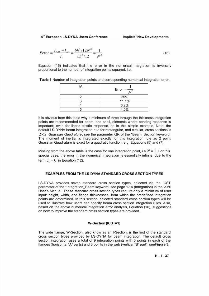
Equation (16) indicates that the error in the numerical integration is inverselyproportional to the number of integration points squared, i.e.

Table 1 Number of integration points and corresponding numerical integration error.

i N

Error 2

1

N =

2 25%

3 11.1%

4 6.2%

5 4.0%

It is obvious from this table why a minimum of three through-the-thickness integrationpoints are recommended for beam, and shell, elements where bending response isimportant; even for linear elastic response, as in this simple example. Note: thedefault LS-DYNA beam integration rule for rectangular, and circular, cross sections is

2 2× Guassian Quadrature, see the parameter QR of the *Beam_Section keyword.The moment of inertial is integrated exactly for this integration rule as 2 pointGuassian Quadrature is exact for a quadratic function, e.g. Equations (5) and (7).

Missing from the above table is the case for one integration point, i.e. 1 N = . For this

special case, the error in the numerical integration is essentially infinite, due to theterm 1

0 z = in Equation (12).

EXAMPLES FROM THE LS-DYNA STANDARD CROSS SECTION TYPES

LS-DYNA provides seven standard cross section types, selected via the ICSTparameter of the *Integration_Beam keyword, see page 17.4 (Integration) in the v960User’s Manual. These standard cross section types require only a minimum of user input: height, width, and flange thicknesses, from which the predefined integrationpoints are determined. In this section, selected standard cross section types will beused to illustrate how users can specify beam cross section integration rules. Also,

based on the above numerical integration error analysis, Equation (16), suggestionson how to improve the standard cross section types are provided.

W-Section (ICST=1)

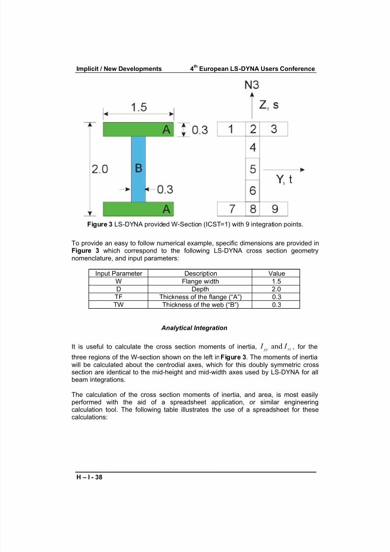
The wide flange, W-Section, also know as an I-Section, is the first of the standardcross section types provided by LS-DYNA for beam integration. The default crosssection integration uses a total of 9 integration points with 3 points in each of theflanges (horizontal “A” parts) and 3 points in the web (vertical “B” part), see Figure 3.

4th


H – I - 37



Figure 3 LS-DYNA provided W-Section (ICST=1) with 9 integration points.

To provide an easy to follow numerical example, specific dimensions are provided inFigure 3 which correspond to the following LS-DYNA cross section geometrynomenclature, and input parameters:

Input Parameter Description Value

W Flange width 1.5

D Depth 2.0TF Thickness of the flange (“A”) 0.3

TW Thickness of the web (“B”) 0.3

Analytical Integration

It is useful to calculate the cross section moments of inertia, and yy zz

I I , for the

three regions of the W-section shown on the left in Figure 3. The moments of inertiawill be calculated about the centrodial axes, which for this doubly symmetric crosssection are identical to the mid-height and mid-width axes used by LS-DYNA for allbeam integrations.

The calculation of the cross section moments of inertia, and area, is most easilyperformed with the aid of a spreadsheet application, or similar engineeringcalculation tool. The following table illustrates the use of a spreadsheet for thesecalculations:



H – I - 38



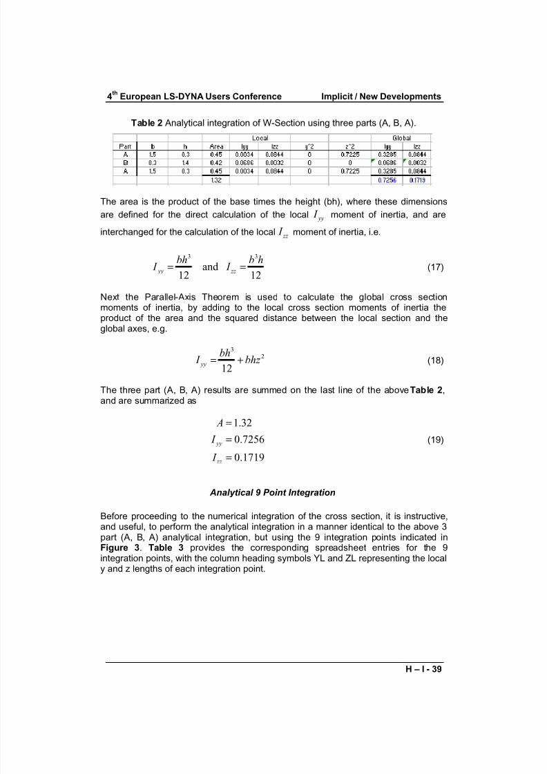
Table 2 Analytical integration of W-Section using three parts (A, B, A).

The area is the product of the base times the height (bh), where these dimensions

are defined for the direct calculation of the local yy I moment of inertia, and are

interchanged for the calculation of the local zz

I moment of inertia, i.e.

3 3

and 12 12 yy zz

bh b h

I I = = (17)

Next the Parallel-Axis Theorem is used to calculate the global cross sectionmoments of inertia, by adding to the local cross section moments of inertia theproduct of the area and the squared distance between the local section and theglobal axes, e.g.

32

12 yy

bh I bhz = + (18)

The three part (A, B, A) results are summed on the last line of the above Table 2,and are summarized as

1.32

0.7256

0.1719

yy

zz

A

I

I

==

=

(19)

Analytical 9 Point Integration

Before proceeding to the numerical integration of the cross section, it is instructive,and useful, to perform the analytical integration in a manner identical to the above 3part (A, B, A) analytical integration, but using the 9 integration points indicated inFigure 3. Table 3 provides the corresponding spreadsheet entries for the 9integration points, with the column heading symbols YL and ZL representing the localy and z lengths of each integration point.

4th


H – I - 39



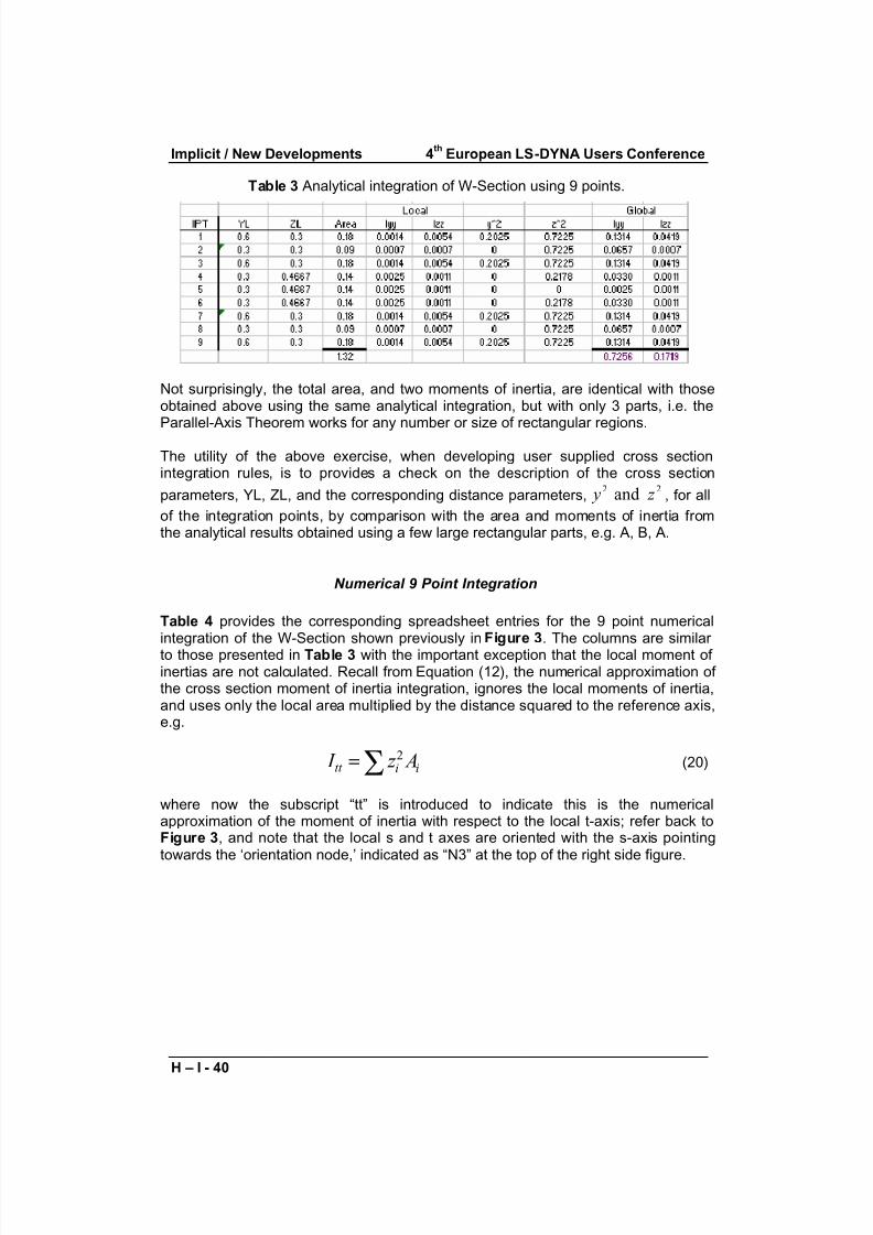
Table 3 Analytical integration of W-Section using 9 points.

Not surprisingly, the total area, and two moments of inertia, are identical with thoseobtained above using the same analytical integration, but with only 3 parts, i.e. theParallel-Axis Theorem works for any number or size of rectangular regions.

The utility of the above exercise, when developing user supplied cross sectionintegration rules, is to provides a check on the description of the cross section

parameters, YL, ZL, and the corresponding distance parameters,2 2 and y z , for all

of the integration points, by comparison with the area and moments of inertia fromthe analytical results obtained using a few large rectangular parts, e.g. A, B, A.

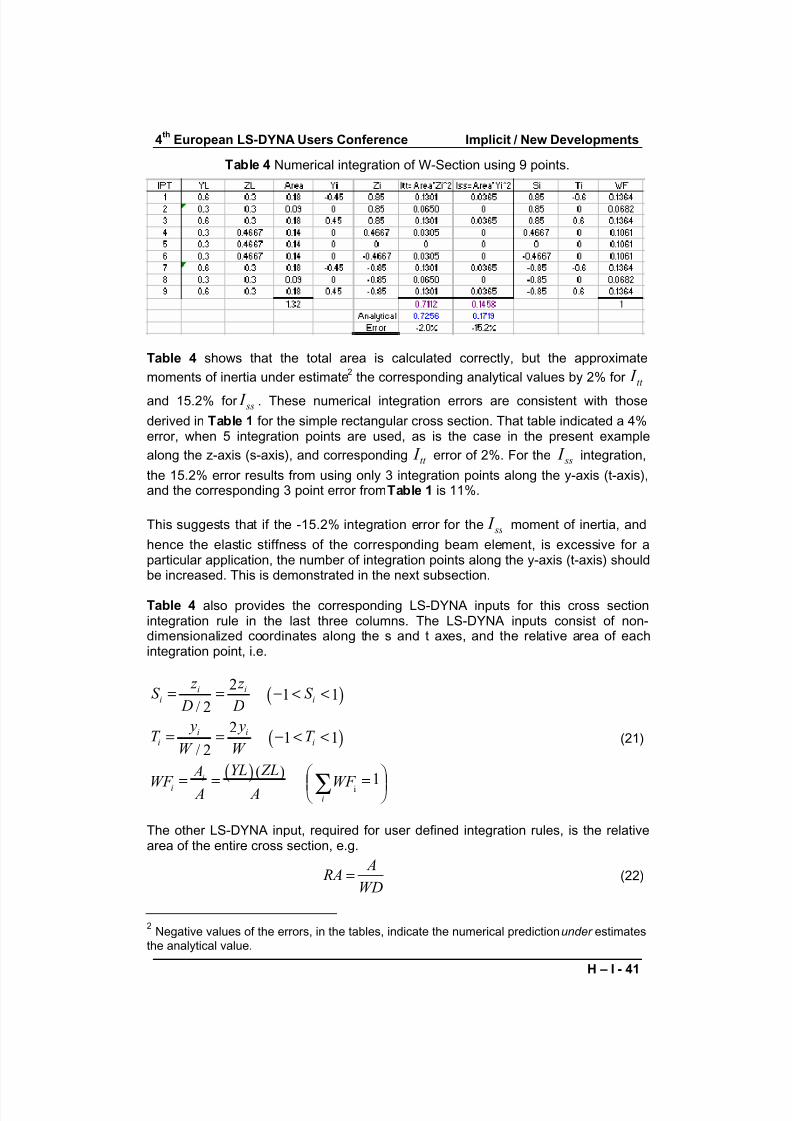
Numerical 9 Point Integration

Table 4 provides the corresponding spreadsheet entries for the 9 point numericalintegration of the W-Section shown previously in Figure 3. The columns are similar to those presented in Table 3 with the important exception that the local moment of inertias are not calculated. Recall from Equation (12), the numerical approximation of the cross section moment of inertia integration, ignores the local moments of inertia,and uses only the local area multiplied by the distance squared to the reference axis,e.g.

2tt i i I z A= ∑ (20)

where now the subscript “tt” is introduced to indicate this is the numericalapproximation of the moment of inertia with respect to the local t-axis; refer back toFigure 3, and note that the local s and t axes are oriented with the s-axis pointingtowards the ‘orientation node,’ indicated as “N3” at the top of the right side figure.



H – I - 40



Table 4 Numerical integration of W-Section using 9 points.

Table 4 shows that the total area is calculated correctly, but the approximate

moments of inertia under estimate2 the corresponding analytical values by 2% for tt I

and 15.2% for ss I . These numerical integration errors are consistent with those

derived in Table 1 for the simple rectangular cross section. That table indicated a 4%error, when 5 integration points are used, as is the case in the present example

along the z-axis (s-axis), and corresponding tt I error of 2%. For the ss I integration,

the 15.2% error results from using only 3 integration points along the y-axis (t-axis),and the corresponding 3 point error from Table 1 is 11%.

This suggests that if the -15.2% integration error for the ss I moment of inertia, and

hence the elastic stiffness of the corresponding beam element, is excessive for aparticular application, the number of integration points along the y-axis (t-axis) shouldbe increased. This is demonstrated in the next subsection.

Table 4 also provides the corresponding LS-DYNA inputs for this cross sectionintegration rule in the last three columns. The LS-DYNA inputs consist of non-dimensionalized coordinates along the s and t axes, and the relative area of eachintegration point, i.e.

( )

( )

( )i

2 1 1

/ 2

2 1 1

/ 2

( )

1

i ii i

i ii i

i

ii

z z S S

D D

y yT T

W W

YL ZL A

WF WF A A

= = − < <

= = − < <

= = = ∑

(21)

The other LS-DYNA input, required for user defined integration rules, is the relativearea of the entire cross section, e.g.

A RA

WD= (22)

2Negative values of the errors, in the tables, indicate the numerical prediction under estimates

the analytical value.

4th


H – I - 41



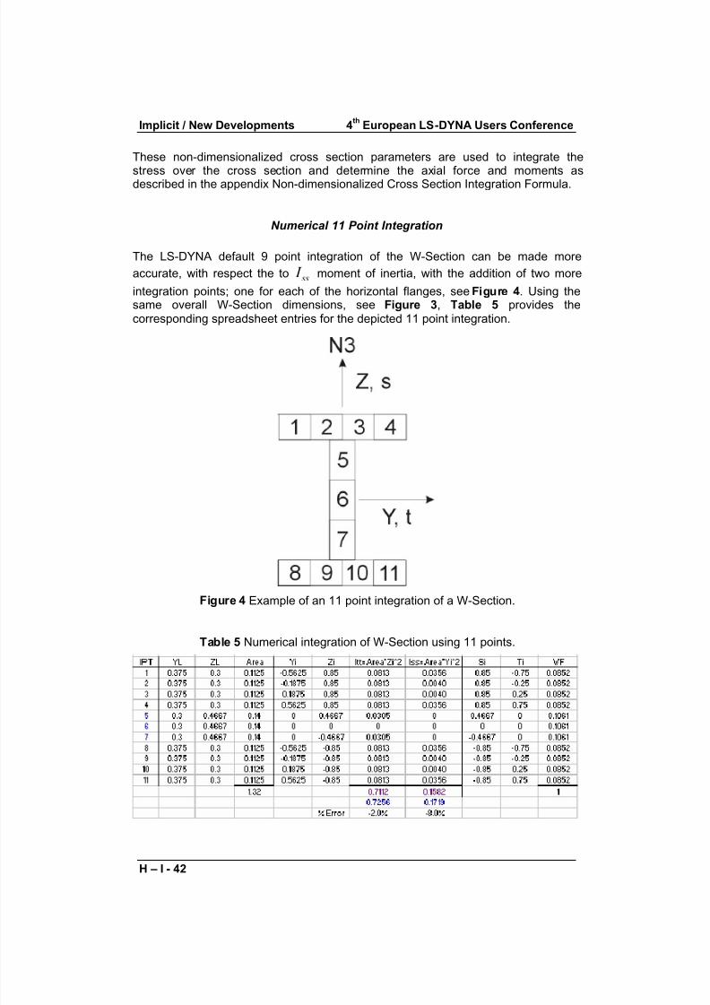
Table 5 indicates the numerical integration error in the ss I moment of inertia isreduced to -8% from the previous -15.2% when 9 integration points were used; e.g. 3points along the y-axis (t-axis). Often in engineering applications, errors on the orderof 10% are acceptable, but the error could be further reduced by adding another twointegration points along the y-axis (t-axis).

The integration template shown in Figure 4 also illustrates that the numericalintegration points do not need to form continuous, or consistent, interfaces of therectangular regions, i.e. there is no need to partition the horizontal flange integrationregions to account for the width of the vertical web, as was done in Figure 3. Further,the numerical integration regions need not be contiguous, i.e. unconnected or isolated integration regions are permitted.

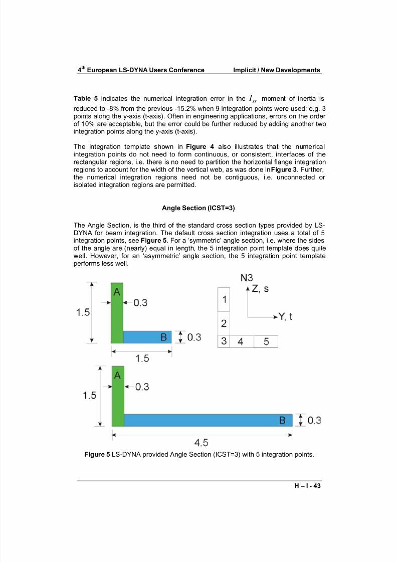
Angle Section (ICST=3)

The Angle Section, is the third of the standard cross section types provided by LS-DYNA for beam integration. The default cross section integration uses a total of 5integration points, see Figure 5. For a ‘symmetric’ angle section, i.e. where the sidesof the angle are (nearly) equal in length, the 5 integration point template does quitewell. However, for an ‘asymmetric’ angle section, the 5 integration point templateperforms less well.

Figure 5 LS-DYNA provided Angle Section (ICST=3) with 5 integration points.

4th


H – I - 43



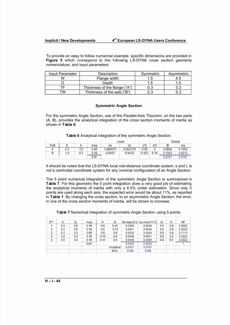
To provide an easy to follow numerical example, specific dimensions are provided inFigure 5 which correspond to the following LS-DYNA cross section geometrynomenclature, and input parameters:

Input Parameter Description Symmetric Asymmetric

W Flange width 1.5 4.5

D Depth 1.5 1.5

TF Thickness of the flange (“A”) 0.3 0.3

TW Thickness of the web (“B”) 0.3 0.3

Symmetric Angle Section

For the symmetric Angle Section, use of the Parallel-Axis Theorem, on the two parts(A, B), provides the analytical integration of the cross section moments of inertia asshown in Table 6.

Table 6 Analytical integration of the symmetric Angle Section.

It should be noted that the LS-DYNA local mid-distance coordinate system, s and t, is

not a centrodial coordinate system for any nominal configuration of an Angle Section.

The 5 point numerical integration of the symmetric Angle Section is summarized inTable 7. For this geometry the 5 point integration does a very good job of estimatingthe analytical moments of inertia with only a 6.5% under estimation. Since only 3points are used along each axis, the expected error would be about 11%, as reportedin Table 1. By changing the cross section, to an asymmetric Angle Section, the error,in one of the cross section moments of inertia, will be shown to increase.

Table 7 Numerical integration of symmetric Angle Section using 5 points.



H – I - 44



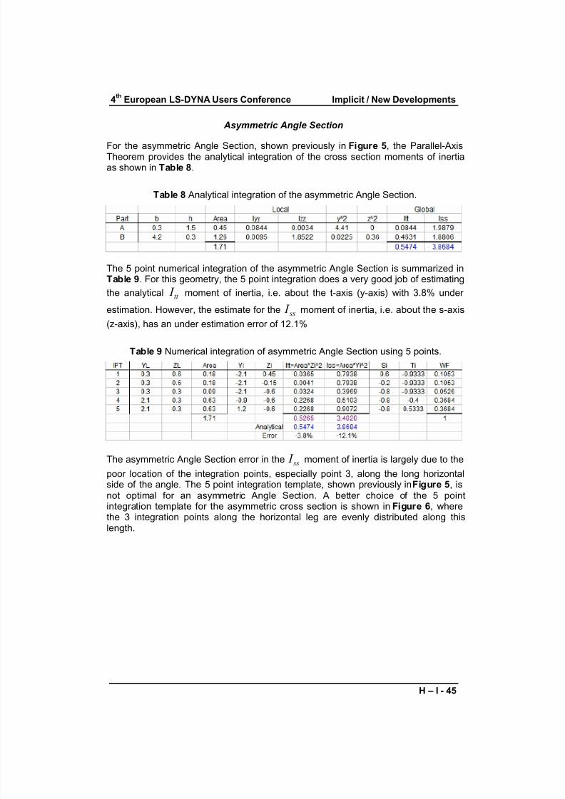
For the asymmetric Angle Section, shown previously in Figure 5, the Parallel-AxisTheorem provides the analytical integration of the cross section moments of inertiaas shown in Table 8.

Table 8 Analytical integration of the asymmetric Angle Section.

The 5 point numerical integration of the asymmetric Angle Section is summarized in

Table 9. For this geometry, the 5 point integration does a very good job of estimatingthe analytical tt I moment of inertia, i.e. about the t-axis (y-axis) with 3.8% under

estimation. However, the estimate for the ss I moment of inertia, i.e. about the s-axis

(z-axis), has an under estimation error of 12.1%

Table 9 Numerical integration of asymmetric Angle Section using 5 points.

The asymmetric Angle Section error in the ss I moment of inertia is largely due to the

poor location of the integration points, especially point 3, along the long horizontalside of the angle. The 5 point integration template, shown previously in Figure 5, isnot optimal for an asymmetric Angle Section. A better choice of the 5 pointintegration template for the asymmetric cross section is shown in Figure 6, wherethe 3 integration points along the horizontal leg are evenly distributed along thislength.

Asymmetric Angle Section

4th


H – I - 45



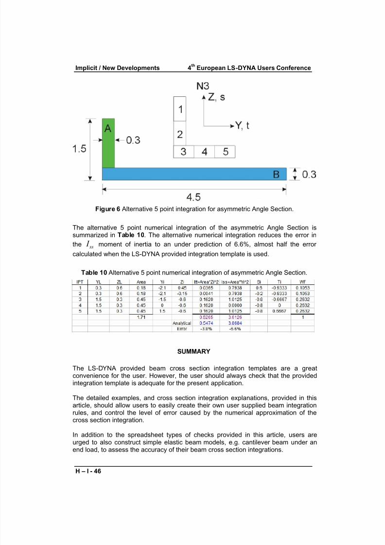
Figure 6 Alternative 5 point integration for asymmetric Angle Section.

The alternative 5 point numerical integration of the asymmetric Angle Section issummarized in Table 10. The alternative numerical integration reduces the error in

the ss I moment of inertia to an under prediction of 6.6%, almost half the error

calculated when the LS-DYNA provided integration template is used.

Table 10 Alternative 5 point numerical integration of asymmetric Angle Section.

SUMMARY

The LS-DYNA provided beam cross section integration templates are a greatconvenience for the user. However, the user should always check that the provided

integration template is adequate for the present application.

The detailed examples, and cross section integration explanations, provided in thisarticle, should allow users to easily create their own user supplied beam integrationrules, and control the level of error caused by the numerical approximation of thecross section integration.

In addition to the spreadsheet types of checks provided in this article, users areurged to also construct simple elastic beam models, e.g. cantilever beam under anend load, to assess the accuracy of their beam cross section integrations.



H – I - 46



APPENDIX NON-DIMENSIONALIZED CROSS SECTION INTEGRATIONFORMULA

The integration of the stress over the cross section to determine the axial force andmoments, uses non-dimensionalized user supplied integration parameters. The user supplied parameters are the non-dimensional coordinates of the integrations points,

i s and it , the relative area of the integration point iWF , and the relative area of the

entire cross section RA ; refer back to Equations (21) and (22) for definitions. Inaddition, the overall cross section dimensions, TS and TT, also need to be providedvia the *Section_Beam keyword; in the W-Section example provided, see Figure 3,TT=W and TS=D.

Using this non-dimensional cross section notation, the area of each integration pointis given by

( )( )( ) ( )i i A WF RA TS TT = (23)

Then the numerical integration for the axial force, Equation (9), and moment,Equation (10), are given by:

( )( )( ) ( )i i i i F dA A RA TS TT WF σ σ σ = ≈ =∑ ∑ ∫ (24)

and

( ) ( ) ( ) ( )

( )( ) ( ) ( )

( )( ) ( ) ( )2

2

1

2

y i i i i i i

i i i

i i i t

M zdA z A RA TS TT z WF

TS RA TS TT s WF

RA TS TT s WF M

σ σ σ

σ

σ

= ≈ =

=

= =

∑ ∑ ∫

∑

∑

(25)

where the moment about the s-axis is obviously

( )( ) ( ) ( )21

2 s i i i

M RA TS TT t WF σ = ∑ (26)

APPENDIX SIMPLE FORMULA FOR INTEGRATION POINTS ON ARECTANGULAR STRIP

Consider a rectangular strip of width W. If the y-coordinate origin is located at themid-width of the strip, i.e. W/2, then for any number integration points N, aligned inthe y-direction, the y-coordinate is given by:

1

2i

N W y i

N

+ = −

4th


H – I - 47





H – I - 48

Ls Dyna Beams

Documents

Transcript of Ls Dyna Beams