AASHTO-LRFD Design Example: Horizontally Curved Steel Box Girder
Upload
waleed-usmanCategory
view
2.343download
38description

LRFD Steel Design
AASHTO LRFD Bridge Design Specifications
Example Problems
Created July 2007


This material is copyrighted by
The University of Cincinnati and
Dr. James A Swanson.
It may not be reproduced, distributed, sold, or stored by any means, electrical or
mechanical, without the expressed written consent of The University of Cincinnati and
Dr. James A Swanson.
July 31, 2007


LRFD Steel Design
AASHTO LRFD Bridge Design Specification
Example Problems Case Study: 2-Span Continuous Bridge.......................................................................................1 Case Study: 1-Span Simply-Supported Bridge .........................................................................63 Case Study: 1-Span Truss Bridge...............................................................................................87 Ad-Hoc Tension Member Examples Tension Member Example #1 ..........................................................................................105 Tension Member Example #2 ..........................................................................................106 Tension Member Example #3 ..........................................................................................108 Tension Member Example #4 ..........................................................................................110 Ad-Hoc Compression Member Examples Compression Member Example #1 .................................................................................111 Compression Member Example #2 .................................................................................112 Compression Member Example #3 .................................................................................114 Compression Member Example #4 .................................................................................116 Compression Member Example #5 .................................................................................119 Compression Member Example #6 .................................................................................121 Compression Member Example #7 .................................................................................123 Ad-Hoc Flexural Member Examples Flexure Example #1 ..........................................................................................................127 Flexure Example #2 ..........................................................................................................129 Flexure Example #3 ..........................................................................................................131 Flexure Example #4 ..........................................................................................................134 Flexure Example #5a ........................................................................................................137 Flexure Example #5b........................................................................................................141 Flexure Example #6a ........................................................................................................147 Flexure Example #6b........................................................................................................152 Ad-Hoc Shear Strength Examples Shear Strength Example #1 .............................................................................................159 Shear Strength Example #2 .............................................................................................161
Ad-Hoc Web Strength and Stiffener Examples Web Strength Example #1 ...............................................................................................165 Web Strength Example #2 ...............................................................................................168 Ad-Hoc Connection and Splice Examples Connection Example #1....................................................................................................175 Connection Example #2....................................................................................................179 Connection Example #3....................................................................................................181 Connection Example #4....................................................................................................182 Connection Example #5....................................................................................................185 Connection Example #6a..................................................................................................187 Connection Example #6b .................................................................................................189 Connection Example #7....................................................................................................190

James A Swanson Associate Professor University of Cincinnati Dept of Civil & Env. Engineering 765 Baldwin Hall Cincinnati, OH 45221-0071
Ph: (513) 556-3774 Fx: (513) 556-2599


2- Span Continuous Bridge Example AASHTO-LRFD 2007 ODOT LRFD Short Course - Steel Page 1 of 62
1. PROBLEM STATEMENT AND ASSUMPTIONS: A two-span continuous composite I-girder bridge has two equal spans of 165’ and a 42’ deck width. The steel girders have Fy = 50ksi and all concrete has a 28-day compressive strength of f’c = 4.5ksi. The concrete slab is 91/2” thick. A typical 2¾” haunch was used in the section properties. Concrete barriers weighing 640plf and an asphalt wearing surface weighing 60psf have also been applied as a composite dead load. HL-93 loading was used per AASHTO (2004), including dynamic load allowance.
3 spaces @ 12' - 0" = 36' - 0" 3'-0"
42' - 0" Out to Out of Deck
39' - 0" Roadway Width
9½” (typ)
23/4" Haunch (typ)
3'-0"
References:
Barth, K.E., Hartnagel, B.A., White, D.W., and Barker, M.G., 2004, “Recommended Procedures for Simplified Inelastic Design of Steel I-Girder Bridges,” ASCE Journal of Bridge Engineering, May/June Vol. 9, No. 3
“Four LRFD Design Examples of Steel Highway Bridges,” Vol. II, Chapter 1A Highway Structures Design Handbook, Published by American Iron and Steel Institute in cooperation with HDR Engineering, Inc. Available at http://www.aisc.org/
-- 1 --

2- Span Continuous Bridge Example AASHTO-LRFD 2007 ODOT LRFD Short Course - Steel Page 2 of 62
Positive Bending Section (Section 1)
Negative Bending Section (Section 2)
2. LOAD CALCULATIONS: DC dead loads (structural components) include:
• Steel girder self weight (DC1) • Concrete deck self weight (DC1) • Haunch self weight (DC1) • Barrier walls (DC2)
DW dead loads (structural attachments) include:
• Wearing surface (DW) 2.1: Dead Load Calculations
Steel Girder Self-Weight (DC1): (Add 15% for Miscellaneous Steel)
(a) Section 1 (Positive Bending)
A = (15”)(3/4”) + (69”)(9/16”) + (21”)(1”) = 71.06 in2
( )( ) Lb
ftinft
2sec 1 2 1.15490 pcf71.06 in 278.1
12tionW
⎛ ⎞⎜ ⎟⎜ ⎟⎜ ⎟⎝ ⎠
= = per girder
(b) Section 2 (Negative Bending) A = (21”)(1”) + (69”)(9/16”) + (21”)(2-1/2”) = 112.3 in2
( )( ) Lb
ftinft
2sec 2 2 1.15490 pcf112.3 in 439.5
12tionW
⎛ ⎞⎜ ⎟⎜ ⎟⎜ ⎟⎝ ⎠
= = per girder
-- 2 --
2- Span Continuous Bridge Example AASHTO-LRFD 2007 ODOT LRFD Short Course - Steel Page 3 of 62
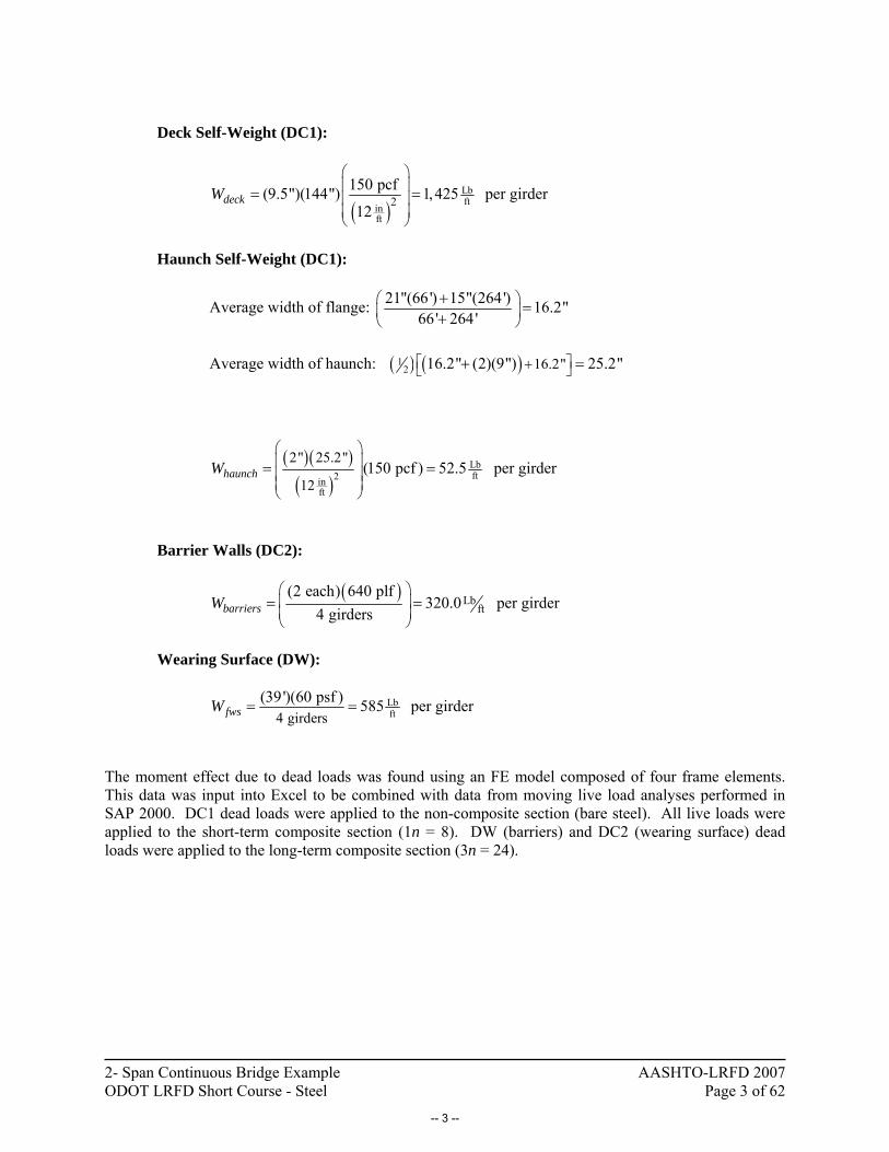
Deck Self-Weight (DC1):
( )Lbft
inft
2150 pcf(9.5")(144") 1,42512
deckW⎛ ⎞⎜ ⎟⎜ ⎟⎜ ⎟⎝ ⎠
= = per girder
Haunch Self-Weight (DC1):
Average width of flange: 21"(66') 15"(264') 16.2"66' 264'
⎛ ⎞⎜ ⎟⎝ ⎠
+ =+
Average width of haunch: ( ) ( )1
2 16.2"16.2" (2)(9") 25.2"⎡ ⎤+⎣ ⎦+ =
( )( )( )
Lbft2in
ft
2" 25.2"
12(150 pcf ) 52.5haunchW
⎛ ⎞⎜ ⎟⎜ ⎟⎜ ⎟⎝ ⎠
= = per girder
Barrier Walls (DC2):
( ) Lbft
(2 each) 640 plf320.0
4 girdersbarriersW⎛ ⎞⎜ ⎟⎜ ⎟⎝ ⎠
= = per girder
Wearing Surface (DW):
Lbft4 girders
(39')(60 psf ) 585fwsW = = per girder
The moment effect due to dead loads was found using an FE model composed of four frame elements. This data was input into Excel to be combined with data from moving live load analyses performed in SAP 2000. DC1 dead loads were applied to the non-composite section (bare steel). All live loads were applied to the short-term composite section (1n = 8). DW (barriers) and DC2 (wearing surface) dead loads were applied to the long-term composite section (3n = 24).
-- 3 --
2- Span Continuous Bridge Example AASHTO-LRFD 2007 ODOT LRFD Short Course - Steel Page 4 of 62
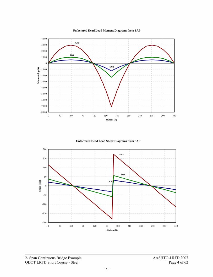
Unfactored Dead Load Moment Diagrams from SAP
-8,000
-7,000
-6,000
-5,000
-4,000
-3,000
-2,000
-1,000
0
1,000
2,000
3,000
4,000
0 30 60 90 120 150 180 210 240 270 300 330
Station (ft)
Mom
ent (
kip-
ft)
DC1
DW
DC2
Unfactored Dead Load Shear Diagrams from SAP
-200
-150
-100
-50
0
50
100
150
200
0 30 60 90 120 150 180 210 240 270 300 330
Station (ft)
Shea
r (k
ip)
DC1
DW
DC2
-- 4 --

2- Span Continuous Bridge Example AASHTO-LRFD 2007 ODOT LRFD Short Course - Steel Page 5 of 62
The following Dead Load results were obtained from the FE analysis:
• The maximum positive live-load moments occur at stations 58.7’ and 271.3’ • The maximum negative live-load moments occur over the center support at station 165.0’
Max (+) Moment Stations 58.7’ and 271.3’
Max (-) Moment Station 165.0’
DC1 - Steel: 475k-ft -1,189k-ft DC1 - Deck: 2,415k-ft -5,708k-ft
DC1 - Haunch: 89k-ft -210k-ft DC1 - Total: 2,979k-ft -7,107k-ft
DC2: 553k-ft -1,251k-ft DW 1,011k-ft -2,286k-ft
-- 5 --

2- Span Continuous Bridge Example AASHTO-LRFD 2007 ODOT LRFD Short Course - Steel Page 6 of 62
2.2: Live Load Calculations The following design vehicular live load cases described in AASHTO-LRFD are considered: 1) The effect of a design tandem combined with the effect of the lane loading. The design tandem consists of two 25kip axles spaced 4.0’ apart. The lane loading consists of a 0.64klf uniform load on all spans of the bridge. (HL-93M in SAP) 2) The effect of one design truck with variable axle spacing combined with the effect of the 0.64klf lane loading. (HL-93K in SAP)
3) For negative moment between points of contraflexure only: 90% of the effect of a truck-train combined with 90% of the effect of the lane loading. The truck train consists of two design trucks (shown below) spaced a minimum of 50’ between the lead axle of one truck and the rear axle of the other truck. The distance between the two 32kip axles should be taken as 14’ for each truck. The points of contraflexure were taken as the field splices at 132’ and 198’ from the left end of the bridge. (HL-93S in SAP)
4) The effect of one design truck with fixed axle spacing used for fatigue loading.
All live load calculations were performed in SAP 2000 using a beam line analysis. The nominal moment data from SAP was then input into Excel. An Impact Factor of 1.33 was applied to the truck and tandem loads and an impact factor of 1.15 was applied to the fatigue loads within SAP.
-- 6 --

2- Span Continuous Bridge Example AASHTO-LRFD 2007 ODOT LRFD Short Course - Steel Page 7 of 62
Unfactored Moving Load Moment Envelopes from SAP
-6,000
-4,000
-2,000
0
2,000
4,000
6,000
0 30 60 90 120 150 180 210 240 270 300 330
Station (ft)
Mom
ent (
kip-
ft)
Single Truck
Tandem
Tandem
Two Trucks
Single Truck
Contraflexure PointContraflexure Point
Fatigue
Fatigue
Unfactored Moving Load Shear Envelopes from SAP
-200
-150
-100
-50
0
50
100
150
200
0 30 60 90 120 150 180 210 240 270 300 330
Station (ft)
Shea
r (k
ip)
Single Truck
Tandem
Fatigue
-- 7 --

2- Span Continuous Bridge Example AASHTO-LRFD 2007 ODOT LRFD Short Course - Steel Page 8 of 62
The following Live Load results were obtained from the SAP analysis:
• The maximum positive live-load moments occur at stations 73.3’ and 256.7’ • The maximum negative live-load moments occur over the center support at station 165.0’
Max (+) Moment Stations 73.3’ and 256’
Max (-) Moment Station 165’
HL-93M 3,725k-ft -3,737k-ft HL-93K 4,396k-ft -4,261k-ft HL-93S N/A -5,317k-ft Fatigue 2,327k-ft -1,095k-ft
Before proceeding, these live-load moments will be confirmed with an influence line analysis.
-- 8 --
2- Span Continuous Bridge Example AASHTO-LRFD 2007 ODOT LRFD Short Course - Steel Page 9 of 62
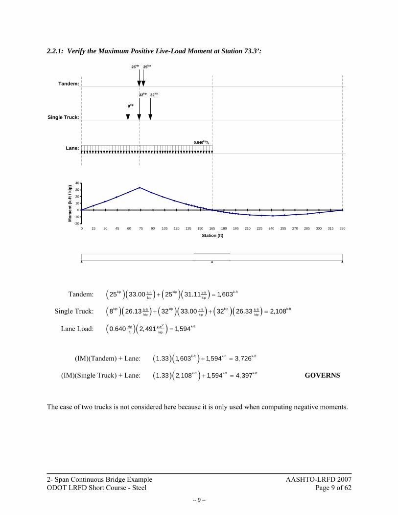
2.2.1: Verify the Maximum Positive Live-Load Moment at Station 73.3’:
Tandem:
Lane:
8kip
32kip 32kip
25kip25kip
0.640kip/ft
Single Truck:
-20
-10
0
10
20
30
40
0 15 30 45 60 75 90 105 120 135 150 165 180 195 210 225 240 255 270 285 300 315 330
Station (ft)
Mom
ent (
k-ft
/ kip
)
Tandem: ( )( ) ( )( )+ =kip kip k-ftk-ft k-ft
kip kip25 33.00 25 31.11 1,603
Single Truck: ( )( ) ( )( ) ( )( )+ + =kip kip kip k-ftk-ft k-ft k-ftkip kip kip
8 26.13 32 33.00 32 26.33 2,108
Lane Load: ( )( ) =2 k-ftkip k-ftft kip
0.640 2,491 1,594
(IM)(Tandem) + Lane: ( )( ) + =k-ft k-ft k-ft1.33 1,603 1,594 3,726
(IM)(Single Truck) + Lane: ( )( ) + =k-ft k-ft k-ft1.33 2,108 1,594 4,397 GOVERNS
The case of two trucks is not considered here because it is only used when computing negative moments.
-- 9 --

2- Span Continuous Bridge Example AASHTO-LRFD 2007 ODOT LRFD Short Course - Steel Page 10 of 62
2.2.2: Verify the Maximum Negative Live-Load Moment at Station 165.0’:
Tandem:
Single Truck:
Lane:
25kip25kip
0.640kip/ft
Two Trucks:
8kip
32kip 32kip
8kip
32kip 32kip
8kip
32kip 32kip
-20
-15
-10
-5
00 15 30 45 60 75 90 105 120 135 150 165 180 195 210 225 240 255 270 285 300 315 330
Station (ft)
Mom
ent (
k-ft
/ kip
)
Tandem: ( )( ) ( )( )+ =kip kip k-ftk-ft k-ft
kip kip25 18.51 25 18.45 924.0
Single Truck: ( )( ) ( )( ) ( )( )+ + =kip kip kip k-ftk-ft k-ft k-ftkip kip kip
8 17.47 32 18.51 32 18.31 1,318
Two Trucks: ( )( ) ( )( ) ( )( )
( )( ) ( )( ) ( )( )+ + +
+ + + =
kip kip kipk-ft k-ft k-ftkip kip kip
kip kip kip k-ftk-ft k-ft k-ftkip kip kip
8 17.47 32 18.51 32 18.31 ...
... 8 16.72 32 18.31 32 18.51 2,630
Lane Load: ( )( ) =2 k-ftkip k-ftft kip
0.640 3,918 2,508
(IM)(Tandem) + Lane: ( )( ) + =k-ft k-ft k-ft1.33 924.0 2,508 3,737
(IM)(Single Truck) + Lane: ( )( ) + =k-ft k-ft k-ft1.33 1,318 2,508 4,261
(0.90){(IM)(Two Trucks) + Lane}: ( ) ( )( ) + =⎡ ⎤⎣ ⎦k-ft k-ft k-ft0.90 1.33 2,630 2,508 5,405 GOVERNS
-- 10 --
2- Span Continuous Bridge Example AASHTO-LRFD 2007 ODOT LRFD Short Course - Steel Page 11 of 62
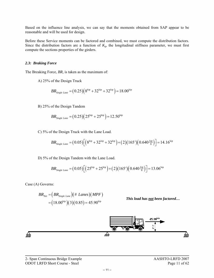
Based on the influence line analysis, we can say that the moments obtained from SAP appear to be reasonable and will be used for design. Before these Service moments can be factored and combined, we must compute the distribution factors. Since the distribution factors are a function of Kg, the longitudinal stiffness parameter, we must first compute the sections properties of the girders. 2.3: Braking Force The Breaking Force, BR, is taken as the maximum of:
A) 25% of the Design Truck ( )( )kip kip kip kip
0.25 8 32 32 18.00Single LaneBR = + + =
B) 25% of the Design Tandem
( )( )kip kip kip 0.25 25 25 12.50Single LaneBR = + =
C) 5% of the Design Truck with the Lane Load. ( ) ( ) ( )( )( )kipkip kip kip kip
ft0.05 8 32 32 2 165' 0.640 14.16Single LaneBR ⎡ ⎤= + + + =⎣ ⎦
D) 5% of the Design Tandem with the Lane Load. ( ) ( ) ( )( )( )kipkip kip kip
ft0.05 25 25 2 165' 0.640 13.06Single LaneBR ⎡ ⎤= + + =⎣ ⎦
Case (A) Governs:
( )( )( )( )( )( )
kip kip
#
18.00 3 0.85 45.90
Net Single LaneBR BR Lanes MPF=
= = This load has not been factored…
-- 11 --

2- Span Continuous Bridge Example AASHTO-LRFD 2007 ODOT LRFD Short Course - Steel Page 12 of 62
2.4: Centrifugal Force A centrifugal force results when a vehicle turns on a structure. Although a centrifugal force doesn’t apply to this bridge since it is straight, the centrifugal load that would result from a hypothetical horizontal curve will be computed to illustrate the procedure. The centrifugal force is computed as the product of the axle loads and the factor, C.
2vC f
gR= (3.6.3-1)
where: v - Highway design speed ( )ft
sec f - 4/3 for all load combinations except for Fatigue, in which case it is 1.0 g - The acceleration of gravity ( )2
ftsec
R - The radius of curvature for the traffic lane (ft). Suppose that we have a radius of R = 600’ and a design speed of v = 65mph = 95.33ft/sec.
( )( )( )2
2ftsec
ftsec
95.334 0.62723 32.2 600 '
C⎡ ⎤⎛ ⎞ ⎢ ⎥= =⎜ ⎟⎢ ⎥⎝ ⎠ ⎣ ⎦
( )( )( )( )( )( )( )( )kip kip
#
72 0.6272 3 0.85 115.2
CE Axle Loads C Lanes MPF=
= =
This force has not been factored… The centrifugal force acts horizontally in the direction pointing away from the center of curvature and at a height of 6’ above the deck. Design the cross frames at the supports to carry this horizontal force into the bearings and design the bearings to resist the horizontal force and the resulting overturning moment.
-- 12 --

2- Span Continuous Bridge Example AASHTO-LRFD 2007 ODOT LRFD Short Course - Steel Page 13 of 62
2.5: Wind Loads For the calculation of wind loads, assume that the bridge is located in the “open country” at an elevation of 40’ above the ground.
Take Z = 40’ Open Country oV = 8.20mph oZ = 0.23ft
Horizontal Wind Load on Structure: (WS) Design Pressure:
2
2 2
mph10,000DZ DZ
D B BB
V VP P PV
⎛ ⎞= =⎜ ⎟
⎝ ⎠ (3.8.1.2.1-1)
PB - Base Pressure - For beams, PB = 50psf when VB = 100mph. (Table 3.8.1.2.1-1)
VB - Base Wind Velocity, typically taken as 100mph. V30 - Wind Velocity at an elevation of Z = 30’ (mph)
VDZ - Design Wind Velocity (mph)
Design Wind Velocity:
( )( )
30
ftmph mph
ft
2.5 ln
100 402.5 8.20 Ln 105.8100 0.23
DZ oB o
V ZV VV Z
⎛ ⎞⎛ ⎞= ⎜ ⎟⎜ ⎟
⎝ ⎠ ⎝ ⎠⎛ ⎞⎛ ⎞= =⎜ ⎟⎜ ⎟
⎝ ⎠ ⎝ ⎠
(3.8.1.1-1)
( ) ( )( )2
2mphpsf psf
mph
105.850 55.92
10,000DP = =
The height of exposure, hexp, for the finished bridge is computed as
71.5" 11.75" 42" 125.3" 10.44 'exph = + + = = The wind load per unit length of the bridge, W, is then computed as:
( )( )psf lbsft55.92 10.44 ' 583.7W = =
Total Wind Load: ( )( )( ) kiplbs
, ft583.7 2 165' 192.6H TotalWS = =
For End Abutments: ( )( )( ) kiplbs 1, ft 2583.7 165' 48.16H AbtWS = =
For Center Pier: ( )( )( )( ) kiplbs 1, ft 2583.7 2 165' 96.31H PierWS = =
PD
hexp
-- 13 --
2- Span Continuous Bridge Example AASHTO-LRFD 2007 ODOT LRFD Short Course - Steel Page 14 of 62
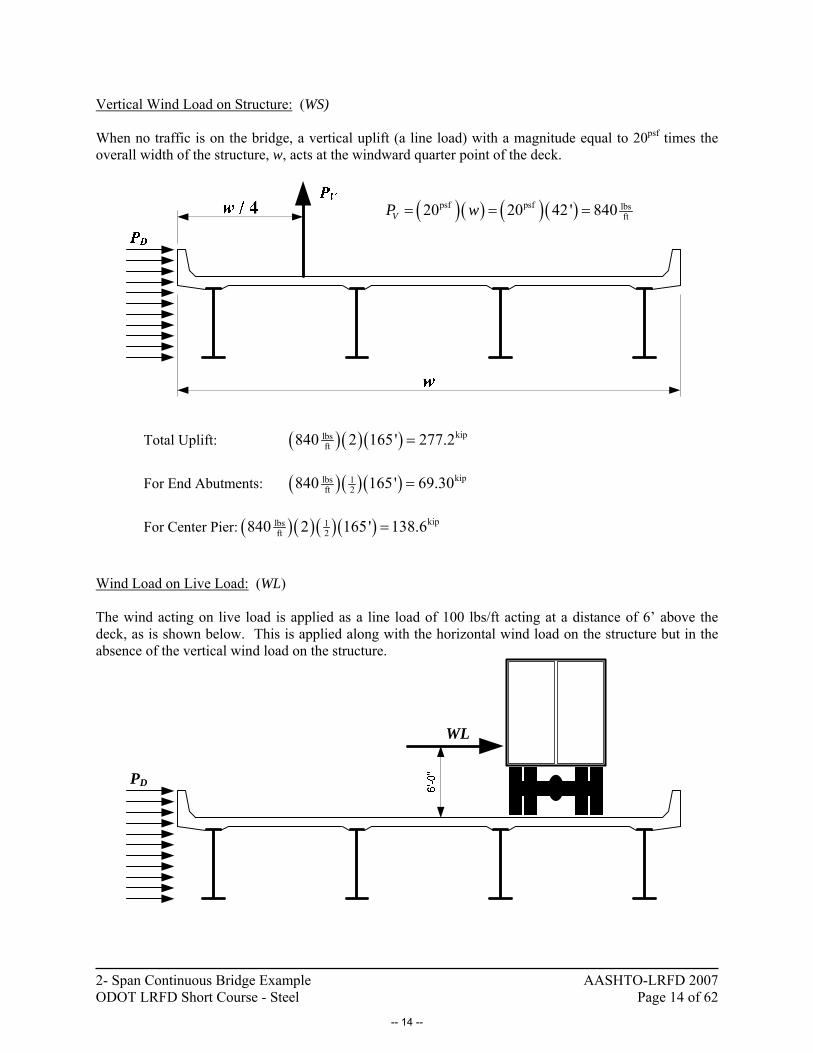
Vertical Wind Load on Structure: (WS) When no traffic is on the bridge, a vertical uplift (a line load) with a magnitude equal to 20psf times the overall width of the structure, w, acts at the windward quarter point of the deck.
( )( ) ( )( )psf psf lbsft20 20 42 ' 840VP w= = =
Total Uplift: ( )( )( ) kiplbs
ft840 2 165' 277.2= For End Abutments: ( )( )( ) kiplbs 1
ft 2840 165' 69.30= For Center Pier: ( )( )( )( ) kiplbs 1
ft 2840 2 165' 138.6= Wind Load on Live Load: (WL) The wind acting on live load is applied as a line load of 100 lbs/ft acting at a distance of 6’ above the deck, as is shown below. This is applied along with the horizontal wind load on the structure but in the absence of the vertical wind load on the structure.
WL
PD
-- 14 --

2- Span Continuous Bridge Example AASHTO-LRFD 2007 ODOT LRFD Short Course - Steel Page 15 of 62
3. SECTION PROPERTIES AND CALCULATIONS: 3.1: Effective Flange Width, beff: For an interior beam, beff is the lesser of:
inft
132' 33' 396"4 4
15"12 (12)(8.5") 109.5"2 2
(12')(12 ) 144"
eff
fs
L
bt
S
⎧• = = =⎪⎪⎪• + = + =⎨⎪• = =⎪⎪⎩
For an exterior beam, beff is the lesser of:
( )inft
132' 33' 198.0"4 4
15"12 (12)(8.5") 109.5"2 2
12' 3' 12 108.0"2 2
eff
fs
e
L
bt
S d
⎧• = = =⎪⎪⎪• + = + =⎨⎪⎪ ⎛ ⎞• + = + =⎪ ⎜ ⎟
⎝ ⎠⎩
Note that Leff was taken as 132.0’ in the above calculations since for the case of effective width in continuous bridges, the span length is taken as the distance from the support to the point of dead load contra flexure. For computing the section properties shown on the two pages that follow, reinforcing steel in the deck was ignored for short-term and long-term composite calculations but was included for the cracked section. The properties for the cracked Section #1 are not used in this example, thus the amount of rebar included is moot. For the properties of cracked Section #2, As = 13.02 in2 located 4.5” from the top of the slab was taken from an underlying example problem first presented by Barth (2004).
-- 15 --
2- Span Continuous Bridge Example AASHTO-LRFD 2007 ODOT LRFD Short Course - Steel Page 16 of 62
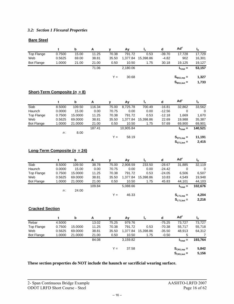
3.2: Section 1 Flexural Properties Bare Steel
t b A y Ay Ix d Ad2 IXTop Flange 0.7500 15.00 11.25 70.38 791.72 0.53 -39.70 17,728 17,729Web 0.5625 69.00 38.81 35.50 1,377.84 15,398.86 -4.82 902 16,301Bot Flange 1.0000 21.00 21.00 0.50 10.50 1.75 30.18 19,125 19,127
71.06 2,180.06 ITotal = 53,157
Y = 30.68 SBS1,top = 1,327SBS1,bot = 1,733
Short-Term Composite (n = 8)
t b A y Ay Ix d Ad2 IXSlab 8.5000 109.50 116.34 75.00 8,725.78 700.49 -16.81 32,862 33,562Haunch 0.0000 15.00 0.00 70.75 0.00 0.00 -12.56 0 0Top Flange 0.7500 15.0000 11.25 70.38 791.72 0.53 -12.18 1,669 1,670Web 0.5625 69.0000 38.81 35.50 1,377.84 15,398.86 22.69 19,988 35,387Bot Flange 1.0000 21.0000 21.00 0.50 10.50 1.75 57.69 69,900 69,901
187.41 10,905.84 ITotal = 140,521n : 8.00
Y = 58.19 SST1,top = 11,191SST1,bot = 2,415
Long-Term Composite (n = 24)
t b A y Ay Ix d Ad2 IXSlab 8.5000 109.50 38.78 75.00 2,908.59 233.50 -28.67 31,885 32,119Haunch 0.0000 15.00 0.00 70.75 0.00 0.00 -24.42 0 0Top Flange 0.7500 15.0000 11.25 70.38 791.72 0.53 -24.05 6,506 6,507Web 0.5625 69.0000 38.81 35.50 1,377.84 15,398.86 10.83 4,549 19,948Bot Flange 1.0000 21.0000 21.00 0.50 10.50 1.75 45.83 44,101 44,103
109.84 5,088.66 ITotal = 102,676n : 24.00
Y = 46.33 SLT1,top = 4,204SLT1,bot = 2,216
Cracked Section
t b A y Ay Ix d Ad2 IXRebar 4.5000 13.02 75.25 979.76 -75.25 73,727 73,727Top Flange 0.7500 15.0000 11.25 70.38 791.72 0.53 -70.38 55,717 55,718Web 0.5625 69.0000 38.81 35.50 1,377.84 15,398.86 -35.50 48,913 64,312Bot Flange 1.0000 21.0000 21.00 0.50 10.50 1.75 -0.50 5 7
84.08 3,159.82 ITotal = 193,764
Y = 37.58 SCR1,top = 5,842SCR1,bot = 5,156
These section properties do NOT include the haunch or sacrificial wearing surface.
-- 16 --

2- Span Continuous Bridge Example AASHTO-LRFD 2007 ODOT LRFD Short Course - Steel Page 17 of 62
3.3: Section 2 Flexural Properties Bare Steel
t b A y Ay Ix d Ad2 IXTop Flange 1.0000 21.00 21.00 72.00 1,512.00 1.75 -45.17 42,841 42,843Web 0.5625 69.00 38.81 37.00 1,436.06 15,398.86 -10.17 4,012 19,411Bot Flange 2.5000 21.00 52.50 1.25 65.63 27.34 25.58 34,361 34,388
112.31 3,013.69 ITotal = 96,642
Y = 26.83 SBS2,top = 2,116SBS2,bot = 3,602
Short Term Composite (n = 8)
t b A y Ay Ix d Ad2 IXSlab 8.5000 109.50 116.34 76.75 8,929.38 700.49 -24.52 69,941 70,641Haunch 0.0000 21.00 0.00 72.50 0.00 0.00 -20.27 0 0Top Flange 1.0000 21.0000 21.00 72.00 1,512.00 1.75 -19.77 8,207 8,208Web 0.5625 69.0000 38.81 37.00 1,436.06 15,398.86 15.23 9,005 24,403Bot Flange 2.5000 21.0000 52.50 1.25 65.63 27.34 50.98 136,454 136,481
228.66 11,943.07 ITotal = 239,734n : 8.00
Y = 52.23 SST2,top = 11,828SST2,bot = 4,590
Long-Term Composite (n = 24)
t b A y Ay Ix d Ad2 IXSlab 8.5000 109.50 38.78 76.75 2,976.46 233.50 -37.10 53,393 53,626Haunch 0.0000 15.00 0.00 72.50 0.00 0.00 -32.85 0 0Top Flange 1.0000 21.0000 21.00 72.00 1,512.00 1.75 -32.35 21,983 21,985Web 0.5625 69.0000 38.81 37.00 1,436.06 15,398.86 2.65 272 15,670Bot Flange 2.5000 21.0000 52.50 1.25 65.63 27.34 38.40 77,395 77,423
151.09 5,990.15 ITotal = 168,704n : 24.00
Y = 39.65 SLT2,top = 5,135SLT2,bot = 4,255
Cracked Section
t b A y Ay Ix d Ad2 IXRebar 4.5000 13.02 77.00 1,002.54 -44.96 26,313 26,313Top Flange 1.0000 21.0000 21.00 72.00 1,512.00 1.75 -39.96 33,525 33,527Web 0.5625 69.0000 38.81 37.00 1,436.06 15,398.86 -4.96 953 16,352Bot Flange 2.5000 21.0000 52.50 1.25 65.63 27.34 30.79 49,786 49,813
125.33 4,016.23 ITotal = 126,006
Y = 32.04 SCR2,top = 3,115SCR2,bot = 3,932
These section properties do NOT include the haunch or sacrificial wearing surface.
-- 17 --

2- Span Continuous Bridge Example AASHTO-LRFD 2007 ODOT LRFD Short Course - Steel Page 18 of 62
4. DISTRIBUTION FACTOR FOR MOMENT 4.1: Positive Moment Region (Section 1): Interior Girder –
One Lane Loaded:
0.10.4 0.3
1, 3
2
4 2 2
4
0.4 0.3 4
1, 3
0.0614 12
( )
8(53,157 in (71.06 in )(46.82") )
1,672, 000 in
12 ' 12 ' 1, 672, 000 in0.06
14 165 ' (12)(165 ')(8.5")
gM Int
s
g g
g
g
M Int
KS SDF
L Lt
K n I Ae
K
K
DF
+
+
= +
= +
= +
=
= +
⎛ ⎞⎛ ⎞ ⎛ ⎞⎜ ⎟⎜ ⎟ ⎜ ⎟ ⎜ ⎟⎝ ⎠ ⎝ ⎠ ⎝ ⎠
⎛⎛ ⎞ ⎛ ⎞⎜⎜ ⎟ ⎜ ⎟
⎝ ⎠ ⎝ ⎠ ⎝
0.1
1, 0.5021M IntDF + =
⎞⎟⎠
In these calculations, the terms eg and Kg include the haunch and sacrificial wearing surface since doing so increases the resulting factor. Note that ts in the denominator of the final term excludes the sacrificial wearing surface since excluding it increases the resulting factor.
Two or More Lanes Loaded:
0.10.6 0.2
2, 3
0.10.6 0.2 4
2, 3
2,
0.0759.5 12
12 ' 12 ' 1,672, 000 in0.075
9.5 165 ' 12(165 ')(8.5")
0.7781
gM Int
s
M Int
M Int
KS SDF
L Lt
DF
DF
+
+
+
= +
= +
=
⎛ ⎞⎛ ⎞ ⎛ ⎞⎜ ⎟⎜ ⎟ ⎜ ⎟ ⎜ ⎟⎝ ⎠ ⎝ ⎠ ⎝ ⎠
⎛ ⎞⎛ ⎞ ⎛ ⎞⎜ ⎟⎜ ⎟ ⎜ ⎟
⎝ ⎠ ⎝ ⎠ ⎝ ⎠
Exterior Girder –
One Lane Loaded:
The lever rule is applied by assuming that a hinge forms over the first interior girder as a truck load is applied near the parapet. The resulting reaction in the exterior girder is the distribution factor.
1,
8.50.7083
12M ExtDF + = =
Multiple Presence: DFM1,Ext+ = (1.2) (0.7083) = 0.8500
-- 18 --

2- Span Continuous Bridge Example AASHTO-LRFD 2007 ODOT LRFD Short Course - Steel Page 19 of 62
Two or More Lanes Loaded:
DFM2,Ext+ = e DFM2,Int+
0.779.11.5
0.77 0.93489.1
ede = +
= + =
DFM2,Ext+ = (0.9348) (0.7781) = 0.7274
4.2: Negative Moment Region (Section 2): The span length used for negative moment near the pier is the average of the lengths of the adjacent spans. In this case, it is the average of 165.0’ and 165.0’ = 165.0’. Interior Girder –
One Lane Loaded:
0.10.4 0.3
1, 3
2
4 2 2
4
0.4 0.3 4
1, 3
0.0614 12
( )
8(96, 642 in (112.3 in )(52.17") )
3, 218, 000 in
12 ' 12 ' 3, 218,000 in0.06
14 165 ' (12)(165 ')(8.5")
gM Int
s
g g
g
g
M Int
KS SDF
L Lt
K n I Ae
K
K
DF
−
−
= +
= +
= +
=
= +
⎛ ⎞⎛ ⎞ ⎛ ⎞⎜ ⎟⎜ ⎟ ⎜ ⎟ ⎜ ⎟⎝ ⎠ ⎝ ⎠ ⎝ ⎠
⎛⎛ ⎞ ⎛ ⎞⎜⎜ ⎟ ⎜ ⎟
⎝ ⎠ ⎝ ⎠ ⎝
0.1
1, 0.5321M IntDF − =
⎞⎟⎠
Two or More Lanes Loaded:
0.10.6 0.2
2, 3
0.10.6 0.2 4
2, 3
2,
0.0759.5 12
12 ' 12 ' 3, 218, 000 in0.075
9.5 165 ' (12)(165 ')(8.5")
0.8257
gM Int
s
M Int
M Int
KS SDF
L Lt
DF
DF
−
−
−
= +
= +
=
⎛ ⎞⎛ ⎞ ⎛ ⎞⎜ ⎟⎜ ⎟ ⎜ ⎟ ⎜ ⎟⎝ ⎠ ⎝ ⎠ ⎝ ⎠
⎛ ⎞⎛ ⎞ ⎛ ⎞⎜ ⎟⎜ ⎟ ⎜ ⎟
⎝ ⎠ ⎝ ⎠ ⎝ ⎠
-- 19 --

2- Span Continuous Bridge Example AASHTO-LRFD 2007 ODOT LRFD Short Course - Steel Page 20 of 62
Exterior Girder – One Lane Loaded:
Same as for the positive moment section: DFM1,Ext- = 0.8500
Two or More Lanes Loaded:
DFM2,Ext- = e DFM2,Int-
0.779.11.5
0.77 0.93489.1
dee = +
= + =
DFM2,Ext- = (0.9348) (0.8257) = 0.7719
4.3: Minimum Exterior Girder Distribution Factor:
,
2
L
Ext Minb
N
ExtL
Nb
X eN
DFN x
= +∑
∑
One Lane Loaded:
1, , 2 2
1 (18.0 ')(14.5 ')0.6125
4 (2) (18 ') (6 ')M Ext MinDF = + =
+⎡ ⎤⎣ ⎦
Multiple Presence: DFM1,Ext,Min = (1.2) (0.6125) = 0.7350
-- 20 --

2- Span Continuous Bridge Example AASHTO-LRFD 2007 ODOT LRFD Short Course - Steel Page 21 of 62
Two Lanes Loaded:
12'3'
2' 3'
14.5'
6'
P1 P2
Lane 1 (12')
3' 2' 3' 3'
2.5'
Lane 2 (12')
2 , , 2 2
2 (18.0 ')(14.5 ' 2.5 ')0.9250
4 (2) (18 ') (6 ')M Ext MinDF
+= + =
+⎡ ⎤⎣ ⎦
Multiple Presence: DFM2,Ext,Min = (1.0) (0.9250) = 0.9250
Three Lanes Loaded:
The case of three lanes loaded is not considered for the minimum exterior distribution factor since the third truck will be placed to the right of the center of gravity of the girders, which will stabilize the rigid body rotation effect resulting in a lower factor.
4.4: Moment Distribution Factor Summary Strength and Service Moment Distribution: Positive Moment Negative Moment Interior Exterior Interior Exterior
1 Lane Loaded: 0.5021 0.8500 ≥ 0.7350 0.5321 0.8500 ≥ 0.7350 2 Lanes Loaded: 0.7781 0.7274 ≥ 0.9250 0.8257 0.7719 ≥ 0.9250
For Simplicity, take the Moment Distribution Factor as 0.9250 everywhere for the Strength and Service load combinations. Fatigue Moment Distribution: For Fatigue, the distribution factor is based on the one-lane-loaded situations with a multiple presence factor of 1.00. Since the multiple presence factor for 1-lane loaded is 1.2, these factors can be obtained by divided the first row of the table above by 1.2. Positive Moment Negative Moment Interior Exterior Interior Exterior
1 Lane Loaded: 0.4184 0.7083 ≥ 0.6125 0.4434 0.7083 ≥ 0.6125 For Simplicity, take the Moment Distribution Factor as 0.7083 everywhere for the Fatigue load combination Multiplying the live load moments by this distribution factor of 0.9250 yields the table of “nominal” girder moments shown on the following page.
-- 21 --
2- Span Continuous Bridge Example AASHTO-LRFD 2007 ODOT LRFD Short Course - Steel Page 22 of 62
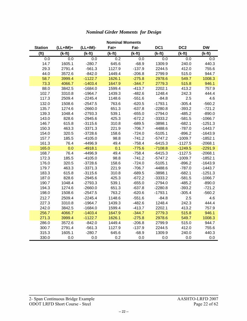
Nominal Girder Moments for Design
Station (LL+IM)+ (LL+IM)- Fat+ Fat- DC1 DC2 DW(ft) (k-ft) (k-ft) (k-ft) (k-ft) (k-ft) (k-ft) (k-ft)
0.0 0.0 0.0 0.2 0.0 0.0 0.0 0.014.7 1605.1 -280.7 645.6 -68.9 1309.9 240.0 440.329.3 2791.4 -561.3 1127.9 -137.9 2244.5 412.0 755.644.0 3572.6 -842.0 1449.4 -206.8 2799.9 515.0 944.758.7 3999.4 -1122.7 1626.1 -275.8 2978.6 549.7 1008.373.3 4066.7 -1403.4 1647.9 -344.7 2779.3 515.8 946.188.0 3842.5 -1684.0 1599.4 -413.7 2202.1 413.2 757.9
102.7 3310.8 -1964.7 1439.3 -482.6 1248.4 242.3 444.4117.3 2509.4 -2245.4 1148.6 -551.6 -84.8 2.5 4.6132.0 1508.6 -2547.5 763.6 -620.5 -1793.1 -305.4 -560.2135.7 1274.6 -2660.0 651.3 -637.8 -2280.8 -393.2 -721.2139.3 1048.4 -2793.3 539.1 -655.0 -2794.0 -485.2 -890.0143.0 828.6 -2945.6 425.3 -672.2 -3333.2 -581.5 -1066.7146.7 615.8 -3115.6 310.8 -689.5 -3898.1 -682.1 -1251.3150.3 463.3 -3371.3 221.9 -706.7 -4488.6 -787.0 -1443.7154.0 320.5 -3728.6 158.6 -724.0 -5105.1 -896.2 -1643.9157.7 185.5 -4105.0 98.8 -741.2 -5747.2 -1009.7 -1852.1161.3 76.4 -4496.9 49.4 -758.4 -6415.3 -1127.5 -2068.1165.0 0.0 -4918.1 0.1 -775.6 -7108.8 -1249.5 -2291.9168.7 76.4 -4496.9 49.4 -758.4 -6415.3 -1127.5 -2068.1172.3 185.5 -4105.0 98.8 -741.2 -5747.2 -1009.7 -1852.1176.0 320.5 -3728.6 158.6 -724.0 -5105.1 -896.2 -1643.9179.7 463.3 -3371.3 221.9 -706.7 -4488.6 -787.0 -1443.7183.3 615.8 -3115.6 310.8 -689.5 -3898.1 -682.1 -1251.3187.0 828.6 -2945.6 425.3 -672.2 -3333.2 -581.5 -1066.7190.7 1048.4 -2793.3 539.1 -655.0 -2794.0 -485.2 -890.0194.3 1274.6 -2660.0 651.3 -637.8 -2280.8 -393.2 -721.2198.0 1508.6 -2547.5 763.2 -620.6 -1793.1 -305.4 -560.2212.7 2509.4 -2245.4 1148.6 -551.6 -84.8 2.5 4.6227.3 3310.8 -1964.7 1439.3 -482.6 1248.4 242.3 444.4242.0 3842.5 -1684.0 1599.4 -413.7 2202.1 413.2 757.9256.7 4066.7 -1403.4 1647.9 -344.7 2779.3 515.8 946.1271.3 3999.4 -1122.7 1626.1 -275.8 2978.6 549.7 1008.3286.0 3572.6 -842.0 1449.4 -206.8 2799.9 515.0 944.7300.7 2791.4 -561.3 1127.9 -137.9 2244.5 412.0 755.6315.3 1605.1 -280.7 645.6 -68.9 1309.9 240.0 440.3330.0 0.0 0.0 0.2 0.0 0.0 0.0 0.0
Nominal Moments
-- 22 --

2- Span Continuous Bridge Example AASHTO-LRFD 2007 ODOT LRFD Short Course - Steel Page 23 of 62
5. DISTRIBUTION FACTOR FOR SHEAR The distribution factors for shear are independent of the section properties and span length. Thus, the only one set of calculations are need - they apply to both the section 1 and section 2 5.1: Interior Girder –
One Lane Loaded:
1 0.3625.012 '0.36 0.840025.0
V ,IntSDF = +
= + =
Two or More Lanes Loaded:
2
2
2
0.212 35
12 ' 12 '0.2 1.08212 35
V ,IntS SDF ⎛ ⎞= + − ⎜ ⎟
⎝ ⎠
⎛ ⎞= + − =⎜ ⎟⎝ ⎠
5.2: Exterior Girder –
One Lane Loaded: Lever Rule, which is the same as for moment: DFV1,Ext = 0.8500 Two or More Lanes Loaded:
DFV2,Ext = e DFV2,Int
0.60101.5 '0.60 0.750010
ede = +
= + =
DFV2,Ext = (0.7500) (1.082) = 0.8115
5.3: Minimum Exterior Girder Distribution Factor - The minimum exterior girder distribution factor applies to shear as well as moment. DFV1,Ext,Min = 0.7350 DFV2,Ext,Min = 0.9250
-- 23 --

2- Span Continuous Bridge Example AASHTO-LRFD 2007 ODOT LRFD Short Course - Steel Page 24 of 62
5.4: Shear Distribution Factor Summary Strength and Service Shear Distribution:
Shear Distribution Interior Exterior
1 Lane Loaded: 0.8400 0.8500 ≥ 0.7350 2 Lanes Loaded: 1.082 0.6300 ≥ 0.9250
For Simplicity, take the Shear Distribution Factor as 1.082 everywhere for Strength and Service load combinations. Fatigue Shear Distribution: For Fatigue, the distribution factor is based on the one-lane-loaded situations with a multiple presence factor of 1.00. Since the multiple presence factor for 1-lane loaded is 1.2, these factors can be obtained by divided the first row of the table above by 1.2.
Shear Distribution Interior Exterior
1 Lane Loaded: 0.7000 0.7083 ≥ 0.6125 For Simplicity, take the Shear Distribution Factor as 0.7083 everywhere for the Fatigue load combination. Multiplying the live load shears by these distribution factors yields the table of “nominal” girder shears shown on the following page.
-- 24 --

2- Span Continuous Bridge Example AASHTO-LRFD 2007 ODOT LRFD Short Course - Steel Page 25 of 62
Nominal Girder Shears for Design
Station (LL+IM)+ (LL+IM)- Fat+ Fat- DC1 DC2 DW(ft) (kip) (kip) (kip) (kip) (kip) (kip) (kip)
0.0 144.9 -19.7 50.8 -4.7 115.0 20.6 37.614.7 123.5 -20.3 44.6 -4.7 88.8 15.9 29.029.3 103.5 -26.8 38.5 -6.4 62.5 11.2 20.544.0 85.0 -41.4 32.6 -11.1 36.3 6.5 11.958.7 68.1 -56.7 26.9 -17.2 10.1 1.8 3.373.3 52.8 -72.7 21.4 -23.2 -16.1 -2.9 -5.388.0 39.4 -89.1 16.3 -29.0 -42.3 -7.6 -13.9
102.7 27.8 -105.7 11.5 -34.6 -68.6 -12.3 -22.4117.3 18.0 -122.3 7.3 -39.9 -94.8 -17.0 -31.0132.0 10.0 -138.6 3.9 -44.9 -121.0 -21.7 -39.6135.7 8.3 -142.5 3.4 -46.0 -127.6 -22.8 -41.7139.3 6.7 -146.5 2.8 -47.2 -134.1 -24.0 -43.9143.0 5.5 -150.5 2.3 -48.3 -140.7 -25.2 -46.0146.7 4.3 -154.5 1.8 -49.4 -147.2 -26.4 -48.2150.3 3.2 -158.4 1.4 -50.4 -153.8 -27.5 -50.3154.0 2.2 -162.3 1.0 -51.5 -160.3 -28.7 -52.5157.7 1.3 -166.2 0.6 -52.4 -166.9 -29.9 -54.6161.3 0.0 -170.1 0.3 -53.4 -173.4 -31.0 -56.8165.0 0.0 -173.9 54.3 -54.3 -180.0 -32.2 -58.9168.7 170.1 -0.5 53.4 -0.3 173.4 31.0 56.8172.3 166.2 -1.3 52.4 -0.6 166.9 29.9 54.6176.0 162.3 -2.2 51.5 -1.0 160.3 28.7 52.5179.7 158.4 -3.2 50.4 -1.4 153.8 27.5 50.3183.3 154.5 -4.3 49.4 -1.8 147.2 26.4 48.2187.0 150.5 -5.5 48.3 -2.3 140.7 25.2 46.0190.7 146.5 -6.7 47.2 -2.8 134.1 24.0 43.9194.3 142.5 -8.3 46.0 -3.4 127.6 22.8 41.7198.0 138.6 -10.0 44.9 -3.9 121.0 21.7 39.6212.7 122.3 -18.0 39.9 -7.3 94.8 17.0 31.0227.3 105.7 -27.8 34.6 -11.5 68.6 12.3 22.4242.0 89.1 -39.4 29.0 -16.3 42.3 7.6 13.9256.7 72.7 -52.8 23.2 -21.4 16.1 2.9 5.3271.3 56.7 -68.1 17.2 -26.9 -10.1 -1.8 -3.3286.0 41.4 -85.0 11.1 -32.6 -36.3 -6.5 -11.9300.7 26.8 -103.5 6.4 -38.5 -62.5 -11.2 -20.5315.3 20.3 -123.5 4.7 -44.6 -88.8 -15.9 -29.0330.0 19.7 -144.9 4.7 -50.8 -115.0 -20.6 -37.6
Nominal Shears
-- 25 --

2- Span Continuous Bridge Example AASHTO-LRFD 2007 ODOT LRFD Short Course - Steel Page 26 of 62
6. FACTORED SHEAR AND MOMENT ENVELOPES
The following load combinations were considered in this example: Strength I: 1.75(LL + IM) + 1.25DC1 + 1.25DC2 + 1.50DW Strength IV: 1.50DC1 + 1.50DC2 + 1.50DW Service II: 1.3(LL + IM) + 1.0DC1 + 1.0DC2 + 1.0DW
Fatigue: 0.75(LL + IM) (IM = 15% for Fatigue; IM = 33% otherwise) Strength II is not considered since this deals with special permit loads. Strength III and V are not considered as they include wind effects, which will be handled separately as needed. Strength IV is considered but is not expected to govern since it addresses situations with high dead load that come into play for longer spans. Extreme Event load combinations are not included as they are also beyond the scope of this example. Service I again applies to wind loads and is not considered (except for deflection) and Service III and Service IV correspond to tension in prestressed concrete elements and are therefore not included in this example. In addition to the factors shown above, a load modifier, η, was applied as is shown below.
i i iQ Qη γ= ∑ η is taken as the product of ηD, ηR, and ηI, and is taken as not less than 0.95. For this example, ηD and ηI are taken as 1.00 while ηR is taken as 1.05 since the bridge has 4 girders with a spacing greater than or equal to 12’. Using these load combinations, the shear and moment envelopes shown on the following pages were developed. Note that for the calculation of the Fatigue moments and shears that η is taken as 1.00 and the distribution factor is based on the one-lane-loaded situations with a multiple presence factor of 1.00 (AASHTO Sections 6.6.1.2.2, Page 6-29 and 3.6.1.4.3b, Page 3-25).
-- 26 --

2- Span Continuous Bridge Example AASHTO-LRFD 2007 ODOT LRFD Short Course - Steel Page 27 of 62
Strength Limit Moment Envelopes
-25,000
-20,000
-15,000
-10,000
-5,000
0
5,000
10,000
15,000
20,000
0 30 60 90 120 150 180 210 240 270 300 330
Station (ft)
Mom
ent (
kip-
ft)
Strength I
Strength IV
Strength IV
Strength I
Strength Limit Shear Force Envelope
-800
-600
-400
-200
0
200
400
600
800
0 30 60 90 120 150 180 210 240 270 300 330
Station (ft)
Shea
r (k
ip)
Strength IV
Strength I
-- 27 --
2- Span Continuous Bridge Example AASHTO-LRFD 2007 ODOT LRFD Short Course - Steel Page 28 of 62
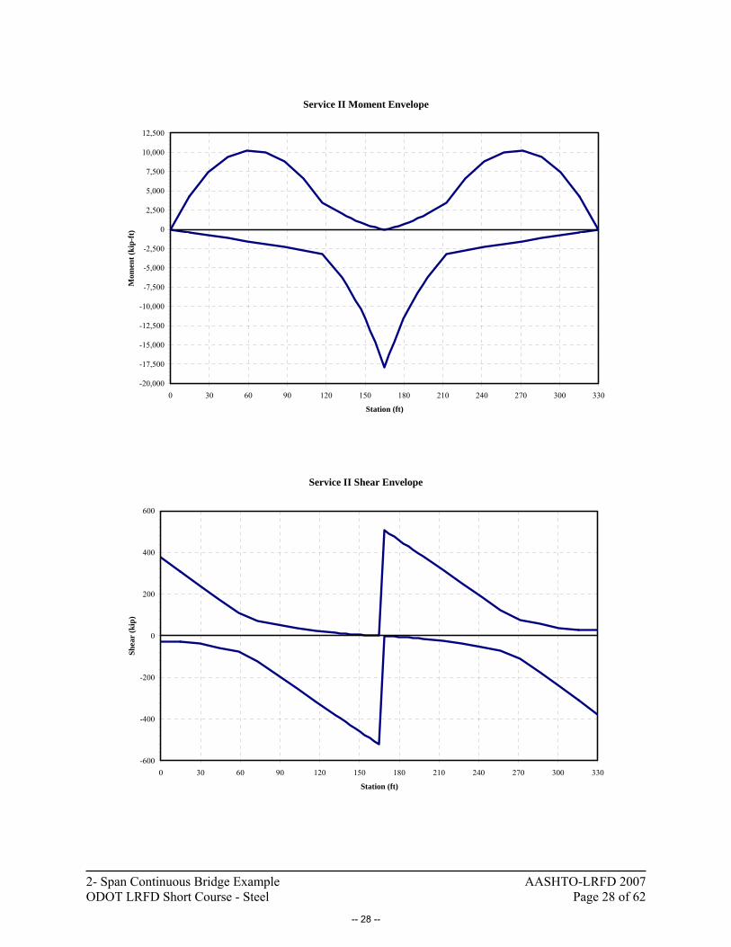
Service II Moment Envelope
-20,000
-17,500
-15,000
-12,500
-10,000
-7,500
-5,000
-2,500
0
2,500
5,000
7,500
10,000
12,500
0 30 60 90 120 150 180 210 240 270 300 330
Station (ft)
Mom
ent (
kip-
ft)
Service II Shear Envelope
-600
-400
-200
0
200
400
600
0 30 60 90 120 150 180 210 240 270 300 330
Station (ft)
Shea
r (k
ip)
-- 28 --
2- Span Continuous Bridge Example AASHTO-LRFD 2007 ODOT LRFD Short Course - Steel Page 29 of 62
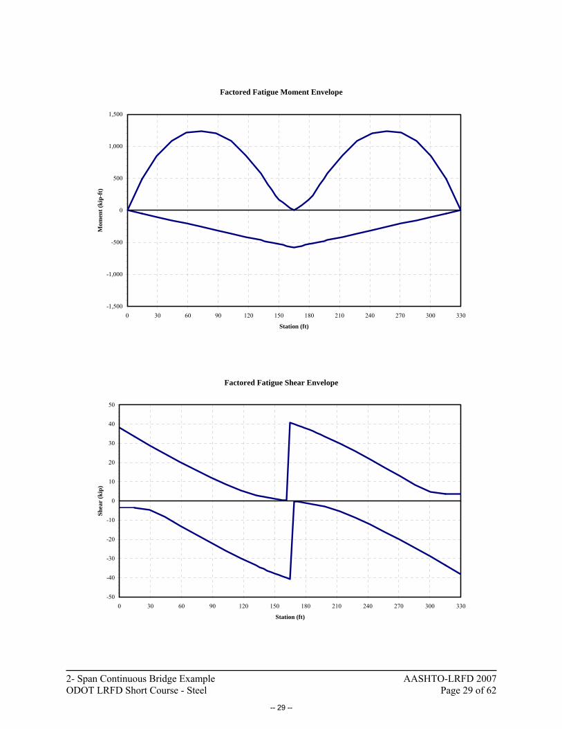
Factored Fatigue Moment Envelope
-1,500
-1,000
-500
0
500
1,000
1,500
0 30 60 90 120 150 180 210 240 270 300 330
Station (ft)
Mom
ent (
kip-
ft)
Factored Fatigue Shear Envelope
-50
-40
-30
-20
-10
0
10
20
30
40
50
0 30 60 90 120 150 180 210 240 270 300 330
Station (ft)
Shea
r (k
ip)
-- 29 --

2- Span Continuous Bridge Example AASHTO-LRFD 2007 ODOT LRFD Short Course - Steel Page 30 of 62
Factored Girder Moments for Design
Station Total + Total - Total + Total - Total + Total - Total + Total -(ft) (k-ft) (k-ft) (k-ft) (k-ft) (k-ft) (k-ft) (k-ft) (k-ft)
0.0 0.0 0.0 0.0 0.0 0.0 0.0 0.2 0.014.7 5677.1 -515.7 3134.6 0.0 4280.7 -383.1 484.2 -51.729.3 9806.0 -1031.5 5374.1 0.0 7393.0 -766.2 845.9 -103.444.0 12403.3 -1547.2 6708.8 0.0 9349.1 -1149.4 1087.1 -155.158.7 13567.8 -2062.9 7145.1 0.0 10222.6 -1532.5 1219.6 -206.873.3 13287.4 -2578.7 6679.8 0.0 10004.2 -1915.6 1235.9 -258.688.0 11687.1 -3094.4 5312.9 0.0 8787.0 -2298.7 1199.5 -310.3
102.7 8740.0 -3610.2 3047.7 0.0 6551.1 -2681.8 1079.5 -362.0117.3 4621.6 -4237.1 11.2 -133.5 3432.8 -3153.9 861.5 -413.7132.0 2772.1 -8317.5 0.0 -4187.3 2059.3 -6268.9 572.7 -465.4135.7 2342.0 -9533.2 0.0 -5347.3 1739.8 -7195.8 488.5 -478.3139.3 1926.4 -10838.2 0.0 -6566.4 1431.1 -8190.4 404.3 -491.3143.0 1522.6 -12230.6 0.0 -7845.7 1131.1 -9251.2 318.9 -504.2146.7 1131.6 -13707.1 0.0 -9184.5 840.6 -10375.8 233.1 -517.1150.3 851.2 -15392.8 0.0 -10582.9 632.3 -11657.1 166.5 -530.0154.0 588.9 -17317.3 0.0 -12041.3 437.4 -13117.1 119.0 -543.0157.7 340.9 -19328.3 0.0 -13559.1 253.3 -14642.7 74.1 -555.9161.3 140.4 -21420.1 0.0 -15137.1 104.3 -16229.6 37.1 -568.8165.0 0.0 -23617.1 0.0 -16774.1 0.0 -17895.9 0.1 -581.7168.7 140.4 -21420.1 0.0 -15137.1 104.3 -16229.6 37.1 -568.8172.3 340.9 -19328.3 0.0 -13559.1 253.3 -14642.7 74.1 -555.9176.0 588.9 -17317.3 0.0 -12041.3 437.4 -13117.1 119.0 -543.0179.7 851.2 -15392.8 0.0 -10582.9 632.3 -11657.1 166.5 -530.0183.3 1131.6 -13707.1 0.0 -9184.5 840.6 -10375.8 233.1 -517.1187.0 1522.6 -12230.6 0.0 -7845.7 1131.1 -9251.2 318.9 -504.2190.7 1926.4 -10838.2 0.0 -6566.4 1431.1 -8190.4 404.3 -491.3194.3 2342.0 -9533.2 0.0 -5347.3 1739.8 -7195.8 488.5 -478.3198.0 2772.1 -8317.5 0.0 -4187.3 2059.3 -6268.9 572.4 -465.4212.7 4621.6 -4237.1 11.2 -133.5 3432.8 -3153.9 861.5 -413.7227.3 8740.0 -3610.2 3047.7 0.0 6551.1 -2681.8 1079.5 -362.0242.0 11687.1 -3094.4 5312.9 0.0 8787.0 -2298.7 1199.5 -310.3256.7 13287.4 -2578.7 6679.8 0.0 10004.2 -1915.6 1235.9 -258.6271.3 13567.8 -2062.9 7145.1 0.0 10222.6 -1532.5 1219.6 -206.8286.0 12403.3 -1547.2 6708.8 0.0 9349.1 -1149.4 1087.1 -155.1300.7 9806.0 -1031.5 5374.1 0.0 7393.0 -766.2 845.9 -103.4315.3 5677.1 -515.7 3134.6 0.0 4280.7 -383.1 484.2 -51.7330.0 0.0 0.0 0.0 0.0 0.0 0.0 0.2 0.0
FatigueStrength I Strength IV Service II
-- 30 --

2- Span Continuous Bridge Example AASHTO-LRFD 2007 ODOT LRFD Short Course - Steel Page 31 of 62
Factored Girder Shears for Design
Station Total + Total - Total + Total - Total + Total - Total + Total -(ft) (kip) (kip) (kip) (kip) (kip) (kip) (kip) (kip)
0.0 479.5 -34.5 272.8 0.0 379.7 -26.9 38.1 -3.514.7 390.5 -35.5 210.6 0.0 309.0 -27.7 33.5 -3.529.3 304.0 -46.9 148.4 0.0 240.2 -36.6 28.9 -4.844.0 220.1 -72.4 86.2 0.0 173.4 -56.5 24.5 -8.358.7 138.9 -99.3 24.0 0.0 108.9 -77.5 20.2 -12.973.3 92.5 -158.9 0.0 -38.2 72.1 -124.8 16.1 -17.488.0 68.9 -239.1 0.0 -100.4 53.8 -188.6 12.2 -21.8
102.7 48.6 -319.7 0.0 -162.6 37.9 -252.7 8.6 -26.0117.3 31.5 -400.1 0.0 -224.8 24.6 -316.8 5.5 -29.9132.0 17.5 -480.2 0.0 -287.0 13.7 -380.5 3.0 -33.7135.7 14.5 -500.0 0.0 -302.6 11.3 -396.3 2.5 -34.5139.3 11.7 -519.8 0.0 -318.1 9.2 -412.1 2.1 -35.4143.0 9.6 -539.7 0.0 -333.7 7.5 -427.9 1.7 -36.2146.7 7.6 -559.6 0.0 -349.2 5.9 -443.7 1.4 -37.0150.3 5.7 -579.3 0.0 -364.8 4.4 -459.4 1.0 -37.8154.0 3.9 -599.0 0.0 -380.3 3.0 -475.1 0.8 -38.6157.7 2.2 -618.7 0.0 -395.9 1.7 -490.8 0.5 -39.3161.3 0.0 -638.3 0.0 -411.4 0.0 -506.4 0.2 -40.0165.0 0.0 -657.9 0.0 -427.0 0.0 -522.0 40.7 -40.7168.7 638.3 -0.9 411.4 0.0 506.4 -0.7 40.0 -0.2172.3 618.7 -2.2 395.9 0.0 490.8 -1.7 39.3 -0.5176.0 599.0 -3.9 380.3 0.0 475.1 -3.0 38.6 -0.8179.7 579.3 -5.7 364.8 0.0 459.4 -4.4 37.8 -1.0183.3 559.6 -7.6 349.2 0.0 443.7 -5.9 37.0 -1.4187.0 539.7 -9.6 333.7 0.0 427.9 -7.5 36.2 -1.7190.7 519.8 -11.7 318.1 0.0 412.1 -9.2 35.4 -2.1194.3 500.0 -14.5 302.6 0.0 396.3 -11.3 34.5 -2.5198.0 480.2 -17.5 287.0 0.0 380.5 -13.7 33.7 -2.9212.7 400.1 -31.5 224.8 0.0 316.8 -24.6 29.9 -5.5227.3 319.7 -48.6 162.6 0.0 252.7 -37.9 26.0 -8.6242.0 239.1 -68.9 100.4 0.0 188.6 -53.8 21.8 -12.2256.7 158.9 -92.5 38.2 0.0 124.8 -72.1 17.4 -16.1271.3 99.3 -138.9 0.0 -24.0 77.5 -108.9 12.9 -20.2286.0 72.4 -220.1 0.0 -86.2 56.5 -173.4 8.3 -24.5300.7 46.9 -304.0 0.0 -148.4 36.6 -240.2 4.8 -28.9315.3 35.5 -390.5 0.0 -210.6 27.7 -309.0 3.5 -33.5330.0 34.5 -479.5 0.0 -272.8 26.9 -379.7 3.5 -38.1
Strength I Strength IV Service II Fatigue
-- 31 --
2- Span Continuous Bridge Example AASHTO-LRFD 2007 ODOT LRFD Short Course - Steel Page 32 of 62
7. FATIGUE CHECKS 7.1: Check transverse stiffener to flange weld at Station 73.3: Traffic information: ADTT given as 2400. Three lanes are available to trucks. (ADTT)SL = (0.80) (2,400) = 1,920 N = (ADTT)SL (365) (75) n = (1,920) (365) (75) (1) = 52.56M Cycles Check Top Flange Weld: Fatigue need only be checked when the compressive stress due to unfactored permanent loads is less than twice the maximum tensile stress due to factored fatigue loads.
Check ?
, 2comp DL Fatf f≤ Distance from bottom of section to the detail under investigation
y = tf,bottom + D = 1.00” + 69.00” = 70”
k-ft1 2,779DCM =
( )( )( )k-ft inft ksi
1 4
2,779 12 70" 30.68"24.67
53,157 inDCf−
= =
k-ft2 515.8DCM =
( )( )( )k-ft inft ksi
2 4
515.8 12 70" 46.33"1.427
102,676 inDCf−
= =
ksi ksi ksi
, 24.67 1.427 26.09comp DLf = + =
k-ft, 258.6Fat NegM =
( )( )( )k-ft inft ksi
4
258.6 12 70" 58.19"0.261
140,521 inFatf−
= =
Check ?
, 2comp DL Fatf f≤ ( )( )?
ksi ksi ksi26.09 2 0.261 0.521≤ = , No. Fatigue need not be checked on the top flange at Station 73.3.
(Pg 24) (Pg 16)
(Pg 16)
(Pg 24) (Pg 16)
(Pg 16)
(Pg 30) (Pg 16)
(Pg 16)
-- 32 --

2- Span Continuous Bridge Example AASHTO-LRFD 2007 ODOT LRFD Short Course - Steel Page 33 of 62
Check Bottom Flange Weld: The permanent loads at Station 73.3 cause tension in the bottom flange, thus by inspection fatigue needs to be checked. ( ) ( )n
f FΔ ≤ Δγ
( ) ( )13
2TH
n
FAFN
Δ⎛ ⎞Δ = ≥⎜ ⎟⎝ ⎠
γ is a load factor of 0.75, which is already included in the fatigue moments.
( ) ( )( )( )k-ft inft ksi
4
1, 236 12 58.19" 1.00"6.036
140,521 infγ
−Δ = =
The detail under consideration is a Category C’ detail. A = 44.0 x 10⁸ ksi3 and (ΔF)TH = 12.0 ksi
( ) ksiksi12.0 6.00
2 2TH
FΔ= = The stress in the detail is almost less than the
infinite life threshold
118 3 33 ksi
6
44 10 ksi 4.37552.56 10
AN
⎛ ⎞×⎛ ⎞ = =⎜ ⎟⎜ ⎟ ×⎝ ⎠ ⎝ ⎠
Since ( )
13 ksi ksi4.375 is less than 6.00
2TH
FAN
Δ⎛ ⎞ = =⎜ ⎟⎝ ⎠
, the infinite life governs.
( ) ksi6.00
nFΔ =
Since ( ) ( )ksi ksi6.036 6.00
nf Fγ Δ = > = , the detail is not satisfactory.
-- 33 --
2- Span Continuous Bridge Example AASHTO-LRFD 2007 ODOT LRFD Short Course - Steel Page 34 of 62
Calculate the design life of the part under consideration:
Since ( ) ( ) is greater than
2TH
Ffγ
ΔΔ , solve for N in the following equation.
( )13Af
Nγ ⎛ ⎞Δ ≤ ⎜ ⎟
⎝ ⎠
( ) ( )8 3
63 3ksi
44 10 ksi 20.01 10 cycles6.036
ANfγ
×≤ = = ×
Δ
620.01 10 cycles 10,420 days
1,920×
=
( )10, 420 days 28.55 years = 28y, 6m, 19d, 2h, 38min...365
= ☺
-- 34 --
2- Span Continuous Bridge Example AASHTO-LRFD 2007 ODOT LRFD Short Course - Steel Page 35 of 62
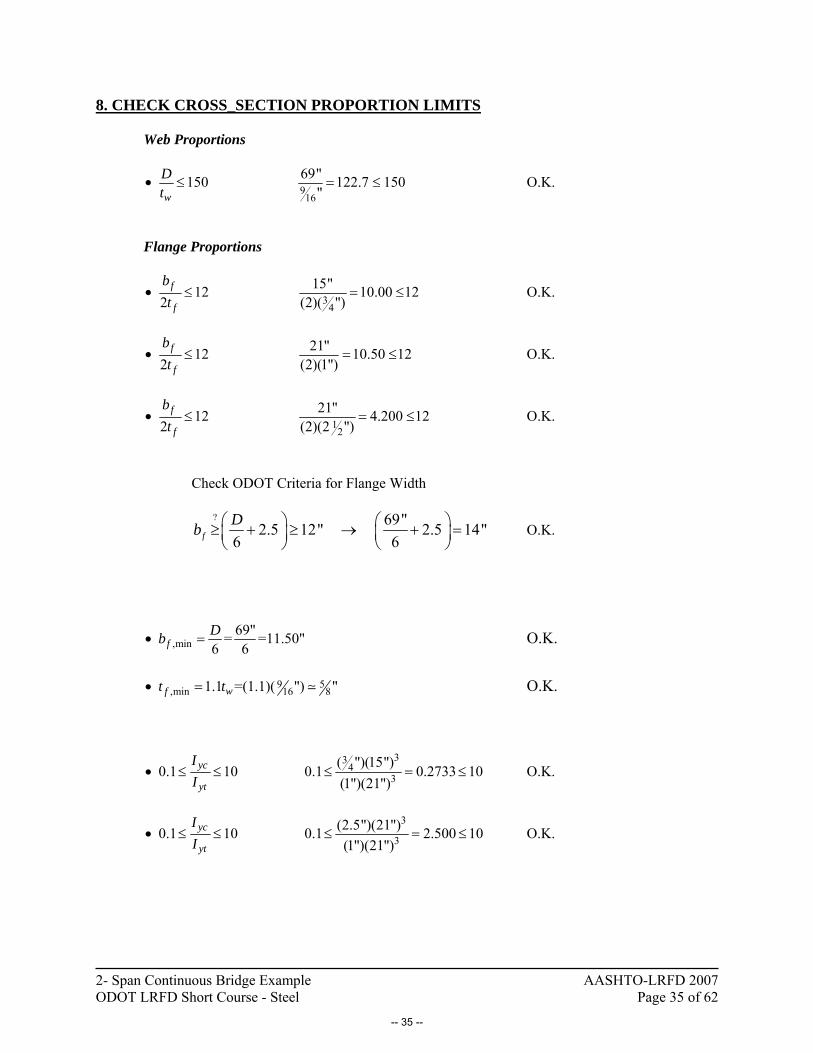
8. CHECK CROSS_SECTION PROPORTION LIMITS
Web Proportions
916
69"150 122.7 150"w
Dt
• ≤ = ≤ O.K.
Flange Proportions
34
15"12 10.00 122 (2)( ")
f
f
bt
• ≤ = ≤ O.K.
21"12 10.50 122 (2)(1")
f
f
bt
• ≤ = ≤ O.K.
1
2
21"12 4.200 122 (2)(2 ")
f
f
bt
• ≤ = ≤ O.K.
Check ODOT Criteria for Flange Width
? 69"2.5 12" 2.5 14"
6 6fDb ⎛ ⎞ ⎛ ⎞≥ + ≥ → + =⎜ ⎟ ⎜ ⎟
⎝ ⎠ ⎝ ⎠ O.K.
,min69"= =11.50"
6 6fDb• = O.K.
9 5
,min 16 81.1 =(1.1)( ") "wft t• = O.K.
33
43
( ")(15")0.1 10 0.1 0.2733 10(1")(21")
yc
yt
II
• ≤ ≤ ≤ = ≤ O.K.
3
3(2.5")(21")0.1 10 0.1 2.500 10(1")(21")
yc
yt
II
• ≤ ≤ ≤ = ≤ O.K.
-- 35 --
2- Span Continuous Bridge Example AASHTO-LRFD 2007 ODOT LRFD Short Course - Steel Page 36 of 62
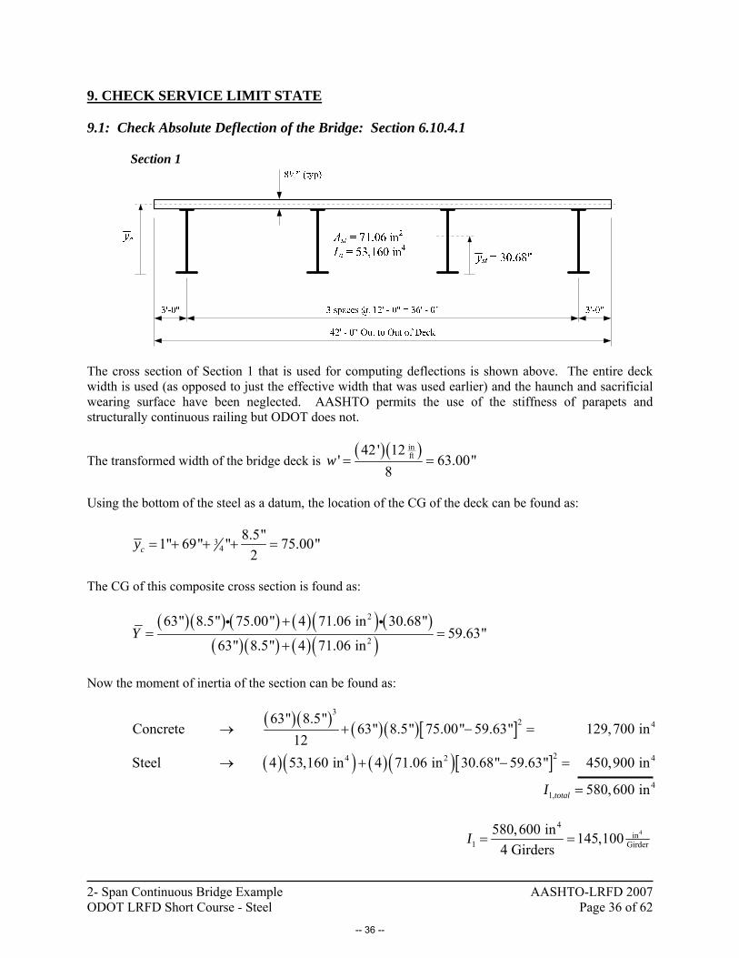
9. CHECK SERVICE LIMIT STATE 9.1: Check Absolute Deflection of the Bridge: Section 6.10.4.1
Section 1
The cross section of Section 1 that is used for computing deflections is shown above. The entire deck width is used (as opposed to just the effective width that was used earlier) and the haunch and sacrificial wearing surface have been neglected. AASHTO permits the use of the stiffness of parapets and structurally continuous railing but ODOT does not.
The transformed width of the bridge deck is ( )( )in
ft42 ' 12' 63.00"
8w = =
Using the bottom of the steel as a datum, the location of the CG of the deck can be found as:
34
8.5"1" 69" " 75.00"2cy = + + + =
The CG of this composite cross section is found as:
( )( ) ( ) ( )( ) ( )
( )( ) ( )( )2
2
63" 8.5" 75.00" 4 71.06 in 30.68"59.63"
63" 8.5" 4 71.06 inY
+= =
+
i i
Now the moment of inertia of the section can be found as:
( )( ) ( )( )[ ]
( )( ) ( )( )[ ]
32 4
24 2 4
41,
63" 8.5"Concrete 63" 8.5" 75.00" 59.63" 129,700 in
12Steel 4 53,160 in 4 71.06 in 30.68" 59.63" 450,900 in
580,600 intotalI
→ + − =
→ + − =
=
44
in1 Girder
580,600 in 145,1004 Girders
I = =
-- 36 --

2- Span Continuous Bridge Example AASHTO-LRFD 2007 ODOT LRFD Short Course - Steel Page 37 of 62
Section 2
The cross section of Section 2 that is used for computing deflections is shown above.
The transformed width of the bridge deck is ( )( )in
ft42 ' 12' 63.00"
8w = =
Using the bottom of the steel as a datum, the location of the CG of the deck can be found as:
12
8.5"2 " 69" 1" 76.75"2cy = + + + =
The CG of this composite cross section is found as:
( )( ) ( ) ( )( ) ( )
( )( ) ( )( )2
2
63" 8.5" 76.75" 4 112.3 in 26.83"53.98"
63" 8.5" 4 112.3 inY
+= =
+
i i
Now the moment of inertia of the section can be found as:
( )( ) ( )( )[ ]
( )( ) ( )( )[ ]
32 4
24 2 4
4
63" 8.5"Concrete 63" 8.5" 76.75" 53.98" 280,900 in
12Steel 4 96,640 in 4 112.3 in 26.83" 53.98" 717,700 in
998,600 intotalI
→ + − =
→ + − =
=
44
in2 Girder
998,600 in 249,7004 Girders
I = =
-- 37 --

2- Span Continuous Bridge Example AASHTO-LRFD 2007 ODOT LRFD Short Course - Steel Page 38 of 62
The following model, which represents the stiffness of a single girder, was used to compute absolute live-load deflections assuming the entire width of the deck to be effective in both compression and tension. The live load component of the Service I load combination is applied. Based on AASHTO Section 3.6.1.3.2, the loading includes (1) the design truck alone and (2) the lane load with 25% of the design truck. The design truck and design lane load were applied separately in the model and will be combined below. The design truck included 33% impact.
I = 145,100 in4 I = 145,100 in4I = 249,700 in4
From the analysis: Deflection due to the Design Truck with Impact: ΔTruck = 2.442” Deflection due to the Design Lane Load: ΔLane = 0.8442” These deflections are taken at Stations 79.2’ and 250.8’. The model was broken into segments roughly 25’ long in the positive moment region and 7’ long in the negative moment region. A higher level of discretization may result in slightly different deflections but it is felt that this level of accuracy was acceptable for deflection calculations. Since the above results are from a single-girder model subjected to one lane’s worth of loading, distribution factors must be applied to obtain actual bridge deflections. Since it is the absolute deflection that is being investigated, all lanes are loaded (multiple presence factor apply) and it is assumed that all girders deflect equally. Given these assumptions, the distribution factor for deflection is simply the number of lanes times the multiple presence factor divided by the number of girders. Looking at the two loading criteria described above:
( )( )( ) ( )
( )( )( ) ( ) ( )( )
1
2
0.85 32.442" 1.558" Governs
4
0.85 30.8442" 0.25 2.442" 0.9274"
4
⎛ ⎞Δ = = ←⎜ ⎟⎜ ⎟
⎝ ⎠⎛ ⎞
Δ = + =⎡ ⎤⎜ ⎟ ⎣ ⎦⎜ ⎟⎝ ⎠
The limiting deflection for this bridge is:
( )( )in
ft165' 122.475" OK
800 800LimitL
Δ = = = ←
-- 38 --

2- Span Continuous Bridge Example AASHTO-LRFD 2007 ODOT LRFD Short Course - Steel Page 39 of 62
9.2: Check the Maximum Span-to-Depth Ratio: Section 6.10.4.1 From Table 2.5.2.6.3-1, (1) the overall depth of a composite I-beam in a continuous span must not be less than 0.032L and (2) the depth of the steel in a composite I-beam in a continuous span must not be less than 0.027L.
( ) ( )( )( )( ) ( )( )( )
inft
inft
1 0.032 0.032 165' 12 63.36" OK
2 0.027 0.027 165' 12 53.46" OK
L
L
→ = =
→ = =
-- 39 --
2- Span Continuous Bridge Example AASHTO-LRFD 2007 ODOT LRFD Short Course - Steel Page 40 of 62
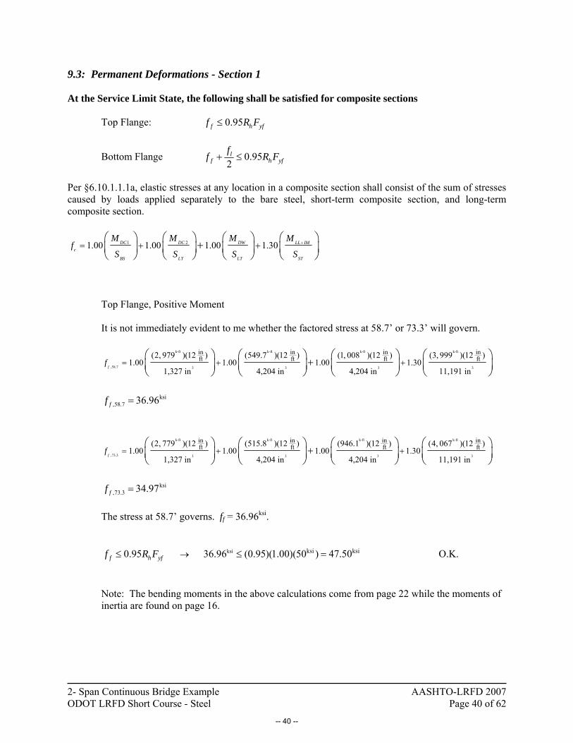
9.3: Permanent Deformations - Section 1 At the Service Limit State, the following shall be satisfied for composite sections Top Flange: 0.95f h yff R F≤
Bottom Flange 0.952
lf h yf
ff R F+ ≤
Per §6.10.1.1.1a, elastic stresses at any location in a composite section shall consist of the sum of stresses caused by loads applied separately to the bare steel, short-term composite section, and long-term composite section.
1 21.00 1.00 1.00 1.30DC DC DW LL IMc
BS LT LT ST
M M M Mf
S S S S+= + +
⎛ ⎞ ⎛ ⎞⎛ ⎞ ⎛ ⎞+⎜ ⎟ ⎜ ⎟⎜ ⎟ ⎜ ⎟
⎝ ⎠ ⎝ ⎠⎝ ⎠ ⎝ ⎠
Top Flange, Positive Moment It is not immediately evident to me whether the factored stress at 58.7’ or 73.3’ will govern.
k-ft k-ft k-ft k-ft
,58.7 3 3 3 3
in in in inft ft ft ft(2, 979 )(12 ) (549.7 )(12 ) (1, 008 )(12 ) (3, 999 )(12 )
1.00 1.00 1.00 1.301,327 in 4,204 in 4,204 in 11,191 in
ff = + ++
⎛ ⎞ ⎛ ⎞ ⎛ ⎞ ⎛ ⎞⎜ ⎟ ⎜ ⎟ ⎜ ⎟ ⎜ ⎟⎝ ⎠ ⎝ ⎠ ⎝ ⎠ ⎝ ⎠
ksi
,58.7 36.96ff =
k-ft k-ft k-ft k-ft
,73.3 3 3 3 3
in in in inft ft ft ft(2, 779 )(12 ) (515.8 )(12 ) (946.1 )(12 ) (4, 067 )(12 )
1.00 1.00 1.00 1.301,327 in 4,204 in 4,204 in 11,191 in
ff = + ++
⎛ ⎞ ⎛ ⎞ ⎛ ⎞ ⎛ ⎞⎜ ⎟ ⎜ ⎟ ⎜ ⎟ ⎜ ⎟⎝ ⎠ ⎝ ⎠ ⎝ ⎠ ⎝ ⎠
ksi
,73.3 34.97ff =
The stress at 58.7’ governs. ff = 36.96ksi.
ksi ksi ksi 0.95 36.96 (0.95)(1.00)(50 ) 47.50f h yff R F →≤ ≤ = O.K.
Note: The bending moments in the above calculations come from page 22 while the moments of inertia are found on page 16.
-- 40 --

2- Span Continuous Bridge Example AASHTO-LRFD 2007 ODOT LRFD Short Course - Steel Page 41 of 62
Bottom Flange, Positive Moment
k-ft k-ft k-ft k-ft
,58.7 3 3 3 3
in in in inft ft ft ft(2, 979 )(12 ) (549.7 )(12 ) (1, 008 )(12 ) (3, 999 )(12 )
1.00 1.00 1.00 1.301,733 in 2,216 in 2,216 in 2,415 in
ff = + ++
⎛ ⎞ ⎛ ⎞ ⎛ ⎞ ⎛ ⎞⎜ ⎟ ⎜ ⎟ ⎜ ⎟ ⎜ ⎟⎝ ⎠ ⎝ ⎠ ⎝ ⎠ ⎝ ⎠
ksi
,58.7 54.90ff =
k-ft k-ft k-ft k-ft
,73.3 3 3 3 3
in in in inft ft ft ft(2, 779 )(12 ) (515.8 )(12 ) (946.1 )(12 ) (4, 067 )(12 )
1.00 1.00 1.00 1.301,733 in 2,216 in 2,216 in 2,415 in
ff = + ++
⎛ ⎞ ⎛ ⎞ ⎛ ⎞ ⎛ ⎞⎜ ⎟ ⎜ ⎟ ⎜ ⎟ ⎜ ⎟⎝ ⎠ ⎝ ⎠ ⎝ ⎠ ⎝ ⎠
ksi
,73.3 53.43ff =
The stress at 58.7’ governs. ff = 54.90ksi. The load factor for wind under Service II is 0.00, ∴ fl = 0ksi
ksi
ksi ksi ksi 54.90 00.95 (0.95)(1.00)(50 ) 47.502 2
lf h yf
ff R F →+ ≤ + ≤ = No Good.
Note: The bending moments in the above calculations come from page 22 while the moments of inertia are found on page 17.
-- 41 --

2- Span Continuous Bridge Example AASHTO-LRFD 2007 ODOT LRFD Short Course - Steel Page 42 of 62
9.4: Permanent Deformations - Section 2
Top Flange, Negative Moment
k-ft k-ft k-ft k-ft
,165 3 3 3 3
in in in inft ft ft ft(7,109 )(12 ) (1, 250 )(12 ) (2, 292 )(12 ) (4, 918 )(12 )
1.00 1.00 1.00 1.302,116 in 5,135 in 5,135 in 11,828 in
ff = + ++
⎛ ⎞ ⎛ ⎞ ⎛ ⎞ ⎛ ⎞⎜ ⎟ ⎜ ⎟ ⎜ ⎟ ⎜ ⎟⎝ ⎠ ⎝ ⎠ ⎝ ⎠ ⎝ ⎠
ksi
,165 55.08ff =
?ksi ksi ksi0.95 55.08 (0.95)(1.00)(50 ) 47.50f h yff R F≤ → ≤ = No Good.
Bottom Flange, Negative Moment
k-ft k-ft k-ft k-ft
3 3 3 3
in in in inft ft ft ft(7,108 )(12 ) (1, 250 )(12 ) (2, 292 )(12 ) (4, 918 )(12 )
1.00 1.00 1.00 1.303,602 in 4,255 in 4,255 in 4,590 in
ff = + ++
⎛ ⎞ ⎛ ⎞ ⎛ ⎞ ⎛ ⎞⎜ ⎟ ⎜ ⎟ ⎜ ⎟ ⎜ ⎟⎝ ⎠ ⎝ ⎠ ⎝ ⎠ ⎝ ⎠
ksi50.39ff =
The load factor for wind under Service II is 0.00, ∴ fl = 0ksi
ksi
ksi ksi ksi00.95 50.39 (0.95)(1.00)(50 ) 47.502 2
lf h yf
ff R F+ ≤ → + ≤ = No Good.
-- 42 --
2- Span Continuous Bridge Example AASHTO-LRFD 2007 ODOT LRFD Short Course - Steel Page 43 of 62
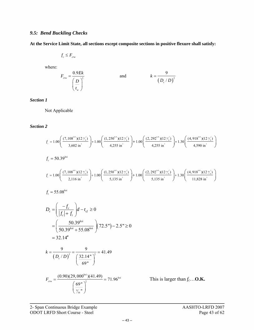
9.5: Bend Buckling Checks At the Service Limit State, all sections except composite sections in positive flexure shall satisfy: c crwf F≤ where:
2
0.9crw
w
EkF
Dt
=⎛ ⎞⎜ ⎟⎝ ⎠
and ( )2
9
/c
kD D
=
Section 1 Not Applicable Section 2
k-ft k-ft k-ft k-ftin in in inft ft ft ft
3 3 3 3
(7,108 )(12 ) (1, 250 )(12 ) (2, 292 )(12 ) (4, 918 )(12 )1.00 1.00 1.00 1.30
3,602 in 4,255 in 4,255 in 4,590 inc
f = + ++⎛ ⎞ ⎛ ⎞ ⎛ ⎞ ⎛ ⎞⎜ ⎟ ⎜ ⎟ ⎜ ⎟ ⎜ ⎟⎝ ⎠ ⎝ ⎠ ⎝ ⎠ ⎝ ⎠
ksi50.39cf =
k-ft k-ft k-ft k-ftin in in in
ft ft ft ft
3 3 3 3
(7,108 )(12 ) (1, 250 )(12 ) (2, 292 )(12 ) (4, 918 )(12 )1.00 1.00 1.00 1.30
2,116 in 5,135 in 5,135 in 11,828 int
f = + ++⎛ ⎞ ⎛ ⎞ ⎛ ⎞ ⎛ ⎞⎜ ⎟ ⎜ ⎟ ⎜ ⎟ ⎜ ⎟⎝ ⎠ ⎝ ⎠ ⎝ ⎠ ⎝ ⎠
ksi55.08tf =
( )ksi
ksi ksi
0
50.39 72.5" 2.5" 050.39 55.08
32.14
cc cf
c t
fD d tf f
⎛ ⎞−= − ≥⎜ ⎟⎜ ⎟+⎝ ⎠⎛ ⎞
= − ≥⎜ ⎟+⎝ ⎠′′=
( )2 2
9 941.49
/ 32.14"69"
c
kD D
= = =⎛ ⎞⎜ ⎟⎝ ⎠
ksi
ksi2
916
(0.90)(29, 000 )(41.49)71.96
69""
crwF = =⎛ ⎞⎜ ⎟⎝ ⎠
This is larger than fc…O.K.
-- 43 --
2- Span Continuous Bridge Example AASHTO-LRFD 2007 ODOT LRFD Short Course - Steel Page 44 of 62
10. CHECK STRENGTH LIMIT STATE 10.1: Section 1 Positive Flexure
Section Classification (§6.10.6.2, Pg. 6.98 – 6.99)
Check 2
3.76cp
w yc
D Et F
≤
Find Dcp, the depth of the web in compression at Mp (compression rebar in the slab is ignored).
( )( )ksi kip
ksi kip916
ksi kip34
' ksi kip
(50 ) 21" 1" 1,050
(50 )(69")( ") 1,941
(50 )(15")( ") 562.5
0.85 (0.85)(4.5 )(109.5")(8.5") 3,560
t yt t t
w yw w
c yc c c
s c s s
P F b t
P F Dt
P F b t
P f b t
= = =
= = =
= = =
= = =
Since Pt + Pw +Pc < Ps 3,554kip < 3,560kip, the PNA lies in the slab.
( ) ( )kip
kip
3,5548.5"3,560
8.486 8.486" from top of slab "
c w ts
s
p
P P PY tP
Y YD
⎡ ⎤ ⎡ ⎤+ +⎢ ⎥ ⎢ ⎥
⎣ ⎦⎣ ⎦
=
= =
= ↓ ∴ =
Since none of the web is in compression, Dcp = 0 and the web is compact. For Composite Sections in Positive Flexure, (§6.10.7.1, Pg. 6.101 – 6.102)
13u xt nl fM f S Mφ+ ≤ Mu = 13,568k-ft from Page 30; take fl = 0
Dt = 1” + 69” + 3/4” + 8.5” = 79.25” 0.1Dt = 7.925” (The haunch is not included in Dt, as per ODOT Exceptions)
Since Dp =8.486 > 0.1Dt = 7.925, 1.07 0.7 pn p
t
DM M
D⎛ ⎞
= −⎜ ⎟⎝ ⎠
kip
k-in k-ft
8.486"(3,554 ) 79.25" 30.68"2
157,500 13,130
pM ⎛ ⎞⎜ ⎟⎝ ⎠
= − −
= =
( ) ( )k-ft k-ft8.486"13,130 1.07 0.7 13,06079.25"nM
⎡ ⎤⎛ ⎞= − =⎜ ⎟⎢ ⎥⎝ ⎠⎣ ⎦
-- 44 --
2- Span Continuous Bridge Example AASHTO-LRFD 2007 ODOT LRFD Short Course - Steel Page 45 of 62
? ?
k-ft k-ft13 (13,568 ) (0) (1.00)(13,060 )u xt nl fM f S Mφ+ ≤ + ≤ No Good.
Note that the check of 1.3 h yn R MM ≤ has not been made in the above calculations. This section would satisfy the Article B6.2 so this check doesn’t need to be made.
Check the ductility requirement to prevent crushing of the slab:
( )( )? ?
0.42 8.486" 0.42 79.25" 33.29"p tD D≤ → ≤ = O.K.
The Section is NOT Adequate for Positive Flexure at Stations 58.7’ and 271.3’
The Girder failed the checks for service limits and has failed the first of several checks at the strength limit state. At this point I will investigate the strength of a section with 70ksi steel in the top and bottom flanges.
-- 45 --
2- Span Continuous Bridge Example AASHTO-LRFD 2007 ODOT LRFD Short Course - Steel Page 46 of 62
Hybrid Girder Factors Will Now be Required: Compute the Hybrid Girder Factor, Rh, for Section 1:
Per AASHTO Commentary Pg 6-95, Dn shall be taken for the bottom flange since this is a composite section in positive flexure.
, 58.19" 1" 57.19"n BottomD = − =
( )312 3
12 2hRβ ρ ρ
β
+ −=
+
( )( )( )( )
916(2) 57.19" "2 3.064
1" 21"n w
fn
D tA
= = =β
ksi
ksi
501.0 0.714370
yw
n
Ff
ρ ρ= ≤ → = =
( )
( )( )
3
, 1
12 3.064 (3)(0.7143) (0.7143)0.9626
12 2 3.064h SectionR⎡ ⎤+ −⎣ ⎦= =+
Compute the Hybrid Girder Factor, Rh, for Section 2: For the short-term composite section, 1
2, 2 " 69" 52.23" 19.27"n TopD = + − =
12, 52.23" 2 " 49.73"n BottomD = − = Governs
( )312 3
12 2hRβ ρ ρ
β
+ −=
+
( )( )( )( )
916
12
(2) 49.73" "2 1.0662 " 21"
n w
fn
D tA
= = =β
ksi
ksi
501.0 0.714370
yw
n
Ff
ρ ρ= ≤ → = =
( )
( )( )
3
, 2
12 1.066 (3)(0.7143) (0.7143)0.9833
12 2 1.066h SectionR⎡ ⎤+ −⎣ ⎦= =+
-- 46 --

2- Span Continuous Bridge Example AASHTO-LRFD 2007 ODOT LRFD Short Course - Steel Page 47 of 62
11. RECHECK SERVICE LIMIT STATE WITH 70KSI FLANGES 11.1: Permanent Deformations - Section 1 At the Service Limit State, the following shall be satisfied for composite sections Top Flange: 0.95f h yff R F≤
Bottom Flange 0.952
lf h yf
ff R F+ ≤
Top Flange, Positive Moment
From before: ksi,58.7 36.96ff =
?
ksi ksi ksi 0.95 36.96 (0.95)(0.9626)(70 ) 64.01f h yff R F →≤ ≤ = O.K.
Bottom Flange, Positive Moment
ksi,58.7 54.90ff = The load factor for wind under Service II is 0.00, ∴ fl = 0ksi
?ksi
ksi ksi ksi 54.90 00.95 (0.95)(0.9626)(70 ) 64.012 2
lf h yf
ff R F →+ ≤ + ≤ = O.K.
11.2: Permanent Deformations - Section 2
Top Flange, Negative Moment
From before: ksi,165 55.08ff =
?
ksi ksi ksi0.95 55.08 (0.95)(0.9833)(70 ) 65.39f h yff R F≤ → ≤ = O.K.
Bottom Flange, Negative Moment
ksi50.39ff = The load factor for wind under Service II is 0.00, ∴ fl = 0ksi
ksi ?ksi ksi ksi00.95 50.39
2 2(0.95)(0.9833)(70 ) 65.39l
f h yff
f R F+ ≤ → + ≤ = O.K.
-- 47 --
2- Span Continuous Bridge Example AASHTO-LRFD 2007 ODOT LRFD Short Course - Steel Page 48 of 62
11.3: Bend Buckling Checks At the Service Limit State, all sections except composite sections in positive flexure shall satisfy: c crwf F≤ where:
2
0.9crw
w
EkF
Dt
=⎛ ⎞⎜ ⎟⎝ ⎠
and ( )2
9
/c
kD D
=
Section 1 - Not Applicable Section 2
k-ft k-ft k-ft k-ftin in in inft ft ft ft
3 3 3 3
(7,108 )(12 ) (1, 250 )(12 ) (2, 292 )(12 ) (4, 918 )(12 )1.00 1.00 1.00 1.30
3,602 in 4,255 in 4,255 in 4,590 inc
f = + ++⎛ ⎞ ⎛ ⎞ ⎛ ⎞ ⎛ ⎞⎜ ⎟ ⎜ ⎟ ⎜ ⎟ ⎜ ⎟⎝ ⎠ ⎝ ⎠ ⎝ ⎠ ⎝ ⎠
ksi50.39cf =
k-ft k-ft k-ft k-ftin in in in
ft ft ft ft
3 3 3 3
(7,108 )(12 ) (1, 250 )(12 ) (2, 292 )(12 ) (4, 918 )(12 )1.00 1.00 1.00 1.30
2,116 in 5,135 in 5,135 in 11,828 int
f = + ++⎛ ⎞ ⎛ ⎞ ⎛ ⎞ ⎛ ⎞⎜ ⎟ ⎜ ⎟ ⎜ ⎟ ⎜ ⎟⎝ ⎠ ⎝ ⎠ ⎝ ⎠ ⎝ ⎠
ksi55.08tf =
( )ksi
ksi ksi
0
50.39 72.5" 2.5" 050.39 55.08
32.14
cc cf
c t
fD d tf f
⎛ ⎞−= − ≥⎜ ⎟⎜ ⎟+⎝ ⎠⎛ ⎞
= − ≥⎜ ⎟+⎝ ⎠′′=
( )2 2
9 941.49
/ 32.14"69"
c
kD D
= = =⎛ ⎞⎜ ⎟⎝ ⎠
ksi
ksi2
916
(0.90)(29, 000 )(41.49)71.96
69""
crwF = =⎛ ⎞⎜ ⎟⎝ ⎠
This is larger than fc…O.K.
-- 48 --
2- Span Continuous Bridge Example AASHTO-LRFD 2007 ODOT LRFD Short Course - Steel Page 49 of 62
12. RECHECK STRENGTH LIMIT STATE WITH 70KSI FLANGES 12.1: Section 1 - Positive Flexure
Section Classification (§6.10.6.2, Pg. 6.98 – 6.99)
Check 2
3.76cp
w yc
D Et F
≤
Find Dcp, the depth of the web in compression at Mp (compression rebar in the slab is ignored).
( )( )ksi kip
ksi kip916
ksi kip34
' ksi kip
(70 ) 21" 1" 1,470
(50 )(69")( ") 1,941
(70 )(15")( ") 787.5
0.85 (0.85)(4.5 )(109.5")(8.5") 3,560
t yt t t
w yw w
c yc c c
s c s s
P F b t
P F Dt
P F b t
P f b t
= = =
= = =
= = =
= = =
Since Pt + Pw +Pc > Ps 4,199kip > 3,560kip, the PNA is NOT in the slab.
Check Case I ?
t w c sP P P P+ ≥ +
?
kip kip kip kip1, 470 1,941 787.5 3,560+ ≥ + NO
Check Case II ?
t w c sP P P P+ + ≥
?
kip kip kip kip1, 470 1,941 787.5 3,560+ + ≥ YES - PNA in Top Flange
kip kip kip
kip
12
0.750" 1,941 1,470 3,560 1 0.3040" (from the top of steel)2 787.5
c w t s
c
t P P PYP
⎛ ⎞+ −⎛ ⎞= +⎜ ⎟⎜ ⎟⎝ ⎠⎝ ⎠
⎛ ⎞+ −⎛ ⎞= + =⎜ ⎟⎜ ⎟⎝ ⎠⎝ ⎠
Dp = 8.5” + 0.3040” = 8.804”
Since none of the web is in compression, Dcp = 0 and the web is compact. For Composite Sections in Positive Flexure, (§6.10.7.1, Pg. 6.101 – 6.102)
13u xt nl fM f S Mφ+ ≤ Mu = 13,568k-ft from Page 30; take fl = 0
Dt = 1” + 69” + 3/4” + 8.5” = 79.25” 0.1Dt = 7.925”
-- 49 --

2- Span Continuous Bridge Example AASHTO-LRFD 2007 ODOT LRFD Short Course - Steel Page 50 of 62
(The haunch is not included in Dt, as per ODOT Exceptions)
Since Dp = 8.804” > 0.1Dt = 7.925”, 1.07 0.7 pn p
t
DM M
D⎛ ⎞
= −⎜ ⎟⎝ ⎠
Determine Mp:
The distances from the component forces to the PNA are calculated.
( )
8.5" 0.3040" 4.554"2
69" 0.75" 0.3040" 34.05"2
1"70.75" 0.3040" 69.95"2
s
w
t
d
d
d
= + =
= − − =
= − − =
The plastic moment is computed.
( ) [ ]
( ) ( )
( )( ) ( )( ) ( )( )
( )
22
kip2 2
kip kip kip
2 k-inkipin
k-
2
787.5 0.3040" 0.750" 0.3040" ...(2)(0.750")
... 3,560 4.554" 1,941 34.05" 1,470 69.95"
525 0.2913 in 185,100
185,300
cp c s s w w t t
c
PM Y t Y P d P d Pdt
⎛ ⎞ ⎡ ⎤= + − + + +⎜ ⎟ ⎣ ⎦⎝ ⎠⎛ ⎞ ⎡ ⎤= + − +⎜ ⎟ ⎣ ⎦⎝ ⎠
⎡ ⎤+ + +⎣ ⎦⎡ ⎤ ⎡ ⎤= +⎣ ⎦ ⎣ ⎦
= in k-ft15,440=
( ) ( )k-ft k-ft8.804"15,440 1.07 0.7 15,32079.25"nM
⎡ ⎤⎛ ⎞= − =⎜ ⎟⎢ ⎥⎝ ⎠⎣ ⎦
? ?
k-ft k-ft13 (13,568 ) (0) (1.00)(15,320 )u xt nl fM f S Mφ+ ≤ + ≤ O.K.
Note that the check of 1.3 h yn R MM ≤ has not been made in the above calculations. This section would satisfy the Article B6.2 so this check doesn’t need to be made.
Check the ductility requirement to prevent crushing of the slab:
( )( )? ?
0.42 8.804" 0.42 79.25" 33.29"p tD D≤ → ≤ = O.K.
The Section is Adequate for Positive Flexure at Stations 58.7’ and 271.3’ with 70ksi Flanges
-- 50 --

2- Span Continuous Bridge Example AASHTO-LRFD 2007 ODOT LRFD Short Course - Steel Page 51 of 62
12.2: Section 2 - Negative Flexure
Section Classification (§6.10.6.2, Pg. 6.98 – 6.99)
Check 2 5.70c
w yc
D Et F
≤
Dc is the depth of the web in compression for the cracked section.
Dc = 32.04” – 21/2” = 29.54”
ksi
ksi916
2 (2)(29.54") 29,000105.0 5.70 5.70 137.3( ") 50
c
w yc
D Et F
= = < = =
The web is non-slender. Since the web is non-slender we have the option of using the provisions in Appendix A to determine the moment capacity. I will first determine the capacity using the provisions in §6.10.8, which will provide a somewhat conservative determination of the flexural resistance. For Composite Sections in Negative Flexure, (§6.10.8.1, Pg. 6.105 – 6.114)
The Compression Flange must satisfy:
13 ncbu l ff f Fφ+ ≤
Per §6.10.1.1.1a, elastic stresses at any location in a composite section shall consist of the sum of stresses caused by loads applied separately to the bare steel, short-term composite section, and long-term composite section. In §6.10.1.1.1c, though, it states that for the Strength Limit, the short-term and long-term composite sections shall consist of the bare steel and the longitudinal rebar. In other words, for determining negative moment stresses over the pier, we can use the factored moment above with the properties for the cracked section.
1 21.25 1.50 1.751.25 DC DC DW LL
buBS CR
M M M Mf
S S−+ +
= +⎛ ⎞ ⎛ ⎞⎜ ⎟ ⎜ ⎟⎝ ⎠ ⎝ ⎠
k-ft k-ft k-ftk-ft
3 3
ininftft
(1.25)(1, 250 ) (1.50)(2, 292 ) (1.75)(4, 918 ) (12 )(7,109 )(12 )1.25
3,602 in 3,932 inbuf+ +
= +⎛ ⎡ ⎤ ⎞⎛ ⎞ ⎣ ⎦⎜ ⎟⎜ ⎟
⎝ ⎠ ⎝ ⎠
ksi71.13buf =
Since fbu is greater than Fyc, it is obvious that a strength computed based on the provisions in §6.10.8 will not be adequate.
-- 51 --

2- Span Continuous Bridge Example AASHTO-LRFD 2007 ODOT LRFD Short Course - Steel Page 52 of 62
As it stands here, this girder is clearly not adequate over the pier. The compression flange is overstressed as per the provisions in §6.10.8. There are still other options to explore, though, before increasing the plate dimensions.
1. Since the web is non-slender for Section 2 in Negative Flexure, we have the option of using the provisions in Appendix A6 to determine moment capacity. This would provide an upper bound strength of Mp instead of My as was determined in §6.10.8.
2. The provisions in Appendix B6 allow for redistribution of negative moment from the region
near the pier to the positive moment region near mid-span for sections that satisfy stringent compactness and stability criteria. If this section qualifies, as much as ~2,000k-ft may be able to be redistributed from the pier to mid-span, which could enable the plastic moment strength from Appendix A6 to be adequate. (This solution may even work with the flange strength at 50ksi, but I doubt it…)
Despite the fact that the girder appears to have failed our flexural capacity checks, let’s look at the shear capacity.
-- 52 --

2- Span Continuous Bridge Example AASHTO-LRFD 2007 ODOT LRFD Short Course - Steel Page 53 of 62
12.3 Vertical Shear Capacity At the strength Limit, the following must be satisfied u nV Vφ≤ For an unstiffened web,
n cr pV V CV= =
Check, 1.12w yw
D Ekt F≤ ,
916
69" 122.7"w
Dt
= =
Since there are no transverse stiffeners, k = 5
ksi
ksi
(29,000 )(5)1.12 60.31(50 )
= ksi
ksi
(29,000 )(5)1.40 75.39(50 )
=
Since 1.40w yw
D Ekt F
> , elastic shear buckling of the web controls.
ksi
2 2 ksi
916
1.57 1.57 (5)(29,000 ) 0.3026(50 )69"
"yw
w
kECFD
t
⎛ ⎞ ⎛ ⎞= = =⎜ ⎟ ⎜ ⎟⎜ ⎟⎛ ⎞ ⎛ ⎞ ⎝ ⎠⎝ ⎠⎜ ⎟ ⎜ ⎟
⎝ ⎠⎝ ⎠
ksi kip9
160.58 (0.58)(50 )(69")( ") 1,126p yw wV F Dt= = =
kip kip(0.3026)(1,126 ) 340.6n pV CV= = =
( )( )kip kip1.00 340.6 340.6nVφ = = No Good.
This strength is adequate from 16’ – 100’ and 230’ - 314’. This strength is not adequate near the end supports or near the pier, however.
-- 53 --

2- Span Continuous Bridge Example AASHTO-LRFD 2007 ODOT LRFD Short Course - Steel Page 54 of 62
Try adding transverse stiffeners spaced at do = 8’ = 96”
2 2
5 55 5 7.58396"69"
o
kdD
= + = + =⎛ ⎞ ⎛ ⎞
⎜ ⎟⎜ ⎟ ⎝ ⎠⎝ ⎠
122.7w
Dt
= , ksi
ksi
(29,000 )(7.583)1.12 74.28(50 )
= , ksi
ksi
(29,000 )(7.583)1.40 92.85(50 )
=
Since 1.40w yw
D Ekt F
> , elastic shear buckling of the web controls.
ksi
2 2 ksi
916
1.57 1.57 (29,000 )(7.583) 0.4589(50 )69"
"yw
w
EkCFD
t
⎛ ⎞ ⎛ ⎞= = =⎜ ⎟ ⎜ ⎟⎜ ⎟⎛ ⎞ ⎛ ⎞ ⎝ ⎠⎝ ⎠⎜ ⎟ ⎜ ⎟
⎝ ⎠⎝ ⎠
kip kip(1.00)(0.4589)(1,126 ) 516.5n pV CVφ = φ = = O.K.
This capacity is fine but we may be able to do better if we account for tension field action. Try adding transverse stiffeners spaced at do = 12’ = 144”
2 2
5 55 5 6.148144"69"
o
kdD
= + = + =⎛ ⎞ ⎛ ⎞
⎜ ⎟⎜ ⎟ ⎝ ⎠⎝ ⎠
122.7w
Dt
= , ksi
ksi
(29,000 )(6.148)1.12 66.88(50 )
= , ksi
ksi
(29,000 )(6.148)1.40 83.60(50 )
=
Since 1.40w yw
D Ekt F
> , elastic shear buckling of the web controls.
ksi
2 2 ksi
916
1.57 1.57 (29,000 )(6.148) 0.3721(50 )69"
"yw
w
EkCFD
t
⎛ ⎞ ⎛ ⎞= = =⎜ ⎟ ⎜ ⎟⎜ ⎟⎛ ⎞ ⎛ ⎞ ⎝ ⎠⎝ ⎠⎜ ⎟ ⎜ ⎟
⎝ ⎠⎝ ⎠
Without TFA: kip kip(0.3721)(1,126 ) 418.9n pV CV= = =
-- 54 --

2- Span Continuous Bridge Example AASHTO-LRFD 2007 ODOT LRFD Short Course - Steel Page 55 of 62
With TFA:
Since ( ) ( )
916
12
2 (2)(69")( ") 1.056 2.5(21")(2 ") (21")(1")
w
fc fc ft ft
Dtb t b t
= = ≤++
,
kip
2 2
0.87(1 ) (0.87)(1 0.3721)(1,126 ) 0.3721144"1169"
n p
o
CV V CdD
⎡ ⎤ ⎡ ⎤⎢ ⎥ ⎢ ⎥
− −⎢ ⎥ ⎢ ⎥= + = +⎢ ⎥ ⎢ ⎥⎛ ⎞ ⎛ ⎞⎢ ⎥ ⎢ ⎥++ ⎜ ⎟⎜ ⎟⎢ ⎥ ⎢ ⎥⎝ ⎠⎝ ⎠ ⎣ ⎦⎣ ⎦
kip kip(1,126 )(0.6082) 684.8nV = =
( )( )kip kip1.00 684.8 684.8nVφ = = O.K.
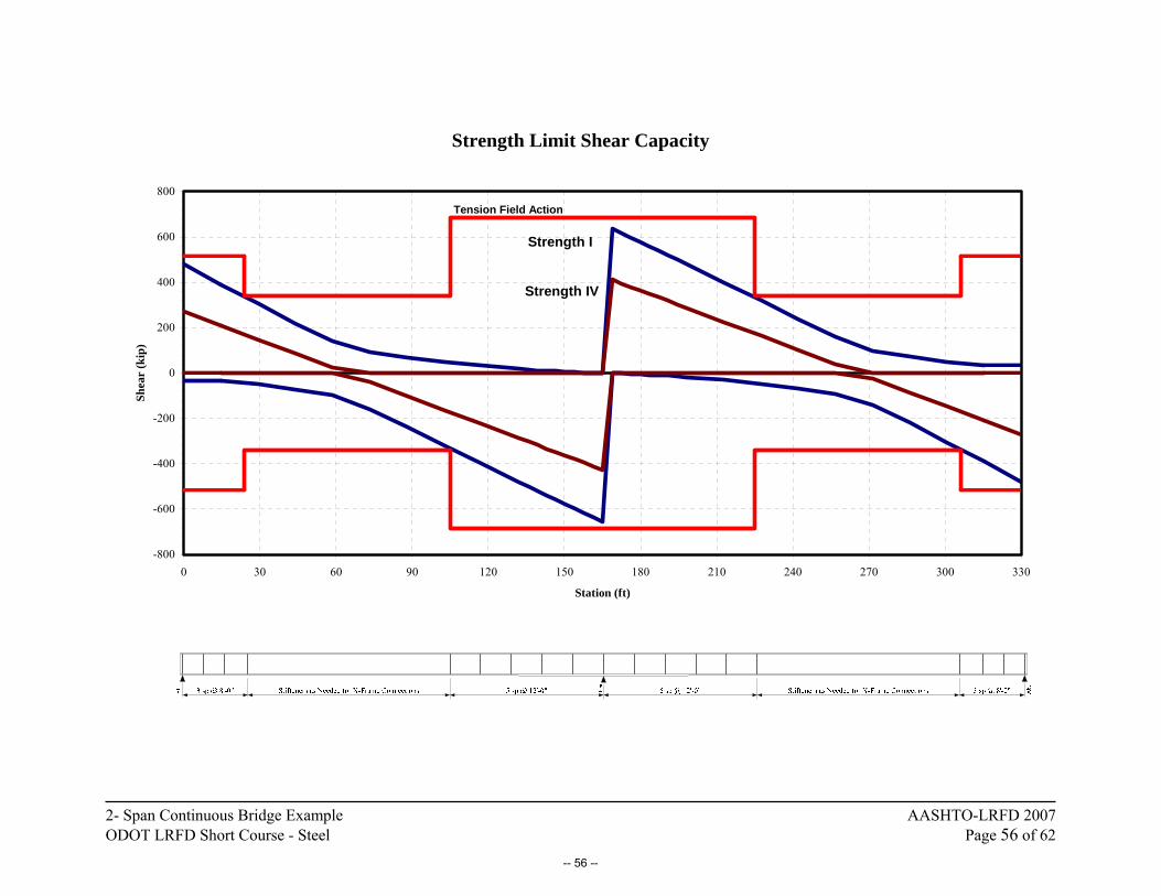
This TFA strength is adequate near the pier but TFA is not permitted in the end panels. The following stiffener configuration should provide adequate shear strength.
-- 55 --
2- Span Continuous Bridge Example AASHTO-LRFD 2007 ODOT LRFD Short Course - Steel Page 56 of 62
Strength Limit Shear Capacity
-800
-600
-400
-200
0
200
400
600
800
0 30 60 90 120 150 180 210 240 270 300 330
Station (ft)
Shea
r (k
ip)
Strength IV
Strength I
Tension Field Action
-- 56 --
2- Span Continuous Bridge Example AASHTO-LRFD 2007 ODOT LRFD Short Course - Steel Page 57 of 62
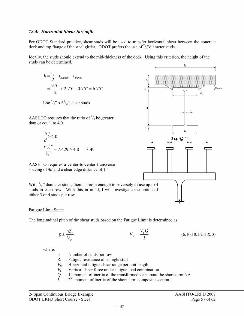
12.4: Horizontal Shear Strength Per ODOT Standard practice, shear studs will be used to transfer horizontal shear between the concrete deck and top flange of the steel girder. ODOT prefers the use of 7/8”diameter studs. Ideally, the studs should extend to the mid-thickness of the deck. Using this criterion, the height of the studs can be determined.
29.5" 2.75" 0.75" 6.75"
2
shaunch flange
th t t= + −
= + − =
Use 7/8” x 61/2” shear studs AASHTO requires that the ratio of h/d be greater than or equal to 4.0.
?
12
78
4.0
6 " 7.429 4.0 OK"
hd≥
= ≥
AASHTO requires a center-to-center transverse spacing of 4d and a clear edge distance of 1”. With 7/8” diameter studs, there is room enough transversely to use up to 4 studs in each row. With this in mind, I will investigate the option of either 3 or 4 studs per row. Fatigue Limit State: The longitudinal pitch of the shear studs based on the Fatigue Limit is determined as
r
sr
nZpV
≤ fsr
V QV
I= (6.10.10.1.2-1 & 3)
where: n - Number of studs per row Zr - Fatigue resistance of a single stud Vsr - Horizontal fatigue shear range per unit length Vf - Vertical shear force under fatigue load combination Q - 1st moment of inertia of the transformed slab about the short-term NA I - 2nd moment of inertia of the short-term composite section
be
ts
bc
bt
tc
D
tt
tw
thaunch
-- 57 --

2- Span Continuous Bridge Example AASHTO-LRFD 2007 ODOT LRFD Short Course - Steel Page 58 of 62
2
2 5.52rdZ dα= ≥ (6.10.10.2-1)
34.5 4.28Log( )Nα = − (6.10.10.2-2) 6 ksi34.5 4.28Log(55.84 10 ) 1.343α = − × =
( )( ) ( )2 2ksi 7 7
8 8
kip kip kip
5.51.343 " "2
1.028 2.105 2.105
r
r
Z
Z
⎛ ⎞= ≥ ⎜ ⎟⎝ ⎠
= ≥ → =
tc cQ A d=
( )( ) 3
1
109.5" 9.5" 9.5"1" 69" 2.75" 58.19" 2,511 in8 2SectionQ
⎡ ⎤ ⎛ ⎞= + + + − =⎢ ⎥ ⎜ ⎟⎝ ⎠⎣ ⎦
( )( ) 3
2
109.5" 9.5" 9.5"2.5" 69" 2.75" 52.23" 3, 481 in8 2SectionQ
⎡ ⎤ ⎛ ⎞= + + + − =⎢ ⎥ ⎜ ⎟⎝ ⎠⎣ ⎦
4
1 140,500 inSectionI = 4 2 239,700 inSectionI =
Since the fatigue shear varies along the length of the bridge, the longitudinal distribution of shear studs based on the Fatigue Limit also varies. These results are presented in a tabular format on a subsequent page. To illustrate the computations, I have chosen the shear at the abutment as an example. At the abutment, ( )kip kip kip38.13 3.53 41.66fV = − − =
( )( )
( )kip 3
kipinch4
41.66 2,511 in0.7445
140,500 insrV = =
For 3 studs in each row: For 4 studs in each row:
( )( )( )
ksiin
rowkipinch
3 2.1058.482
0.7445p ≤ =
( )( )( )
ksiin
rowkipinch
4 2.10511.31
0.7453p ≤ =
-- 58 --
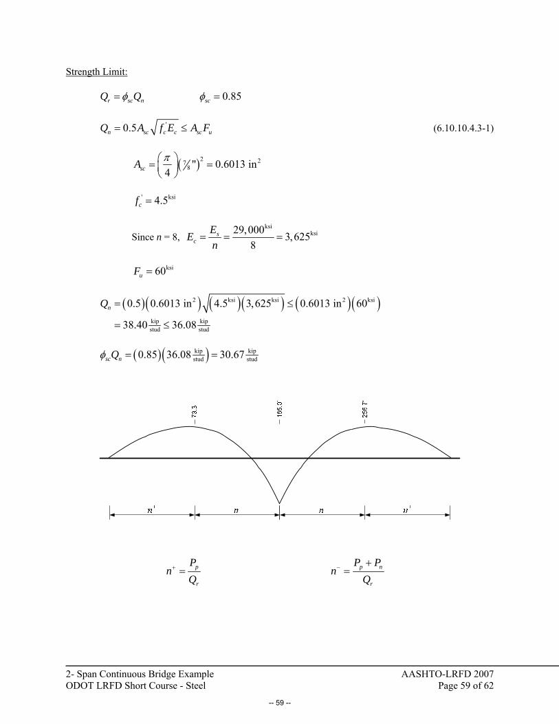
2- Span Continuous Bridge Example AASHTO-LRFD 2007 ODOT LRFD Short Course - Steel Page 59 of 62
Strength Limit: 0.85r sc n scQ Qφ φ= =
'0.5n sc c c sc uQ A f E A F= ≤ (6.10.10.4.3-1)
( )2 278 " 0.6013 in
4scA π⎛ ⎞= =⎜ ⎟⎝ ⎠
' ksi4.5cf =
Since n = 8, ksi
ksi29,000 3,6258
sc
EEn
= = =
ksi60uF =
( )( ) ( )( ) ( )( )2 ksi ksi 2 ksi
kip kipstud stud
0.5 0.6013 in 4.5 3,625 0.6013 in 60
38.40 36.08
nQ = ≤
= ≤
( )( )kip kip
stud stud0.85 36.08 30.67sc nQφ = =
p
r
Pn
Q+ = p n
r
P Pn
Q− +=
-- 59 --
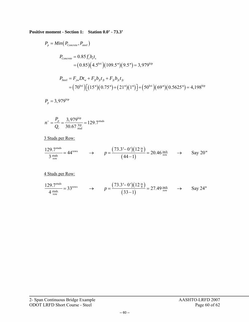
2- Span Continuous Bridge Example AASHTO-LRFD 2007 ODOT LRFD Short Course - Steel Page 60 of 62
Positive moment - Section 1: Station 0.0’ - 73.3’ ( ),p Concrete steelP Min P P=
( )( )( )( )
'
ksi kip
0.85
0.85 4.5 109.5" 9.5" 3,979Concrete c e sP f b t=
= =
( ) ( )( ) ( )( ) ( )( )( )ksi ksi kip70 15" 0.75" 21" 1" 50 69" 0.5625" 4,198Steel yw w ft ft ft fc fc fcP F Dt F b t F b t= + +
= + + =⎡ ⎤⎣ ⎦
kip3,979pP =
kip
studskipstud
3,979 129.730.67
p
r
Pn
Q+ = = =
3 Studs per Row:
( )( )
( )studs in
ftrows inchrowstuds
row
73.3' 0 ' 12129.7 44 20.46 Say 20"3 44 1
p−
= → = = →−
4 Studs per Row:
( )( )
( )studs in
ftrows inchrowstuds
row
73.3' 0 ' 12129.7 33 27.49 Say 24"4 33 1
p−
= → = = →−
-- 60 --

2- Span Continuous Bridge Example AASHTO-LRFD 2007 ODOT LRFD Short Course - Steel Page 61 of 62
Negative Moment - Section 2: Station 73.3’ - 165.0’ ( ),n steel CrackP Min P P=
( )( )( )( )
'
ksi kip
0.45
0.45 4.5 109.5" 9.5" 2,107Crack c e sP f b t=
= =
( ) ( )( ) ( )( ) ( )( )( )ksi ksi kip70 21" 2.5" 21" 1" 50 69" 0.5625" 7,086Steel yw w ft ft ft fc fc fcP F Dt F b t F b t= + +
= + + =⎡ ⎤⎣ ⎦
kip2,107nP =
kip kip
studskipstud
3,979 2,107 198.430.67
p n
r
P Pn
Q− + += = =
3 Studs per Row:
( )( )
( )studs in
ftrows inchrowstuds
row
165.0 ' 73.3' 12198.4 67 16.67 Say 16"3 67 1
p−
= → = = →−
4 Studs per Row:
( )( )
( )studs in
ftrows inchrowstuds
row
165.0 ' 73.3' 12198.4 50 22.48 Say 20"4 50 1
p−
= → = = →−
-- 61 --
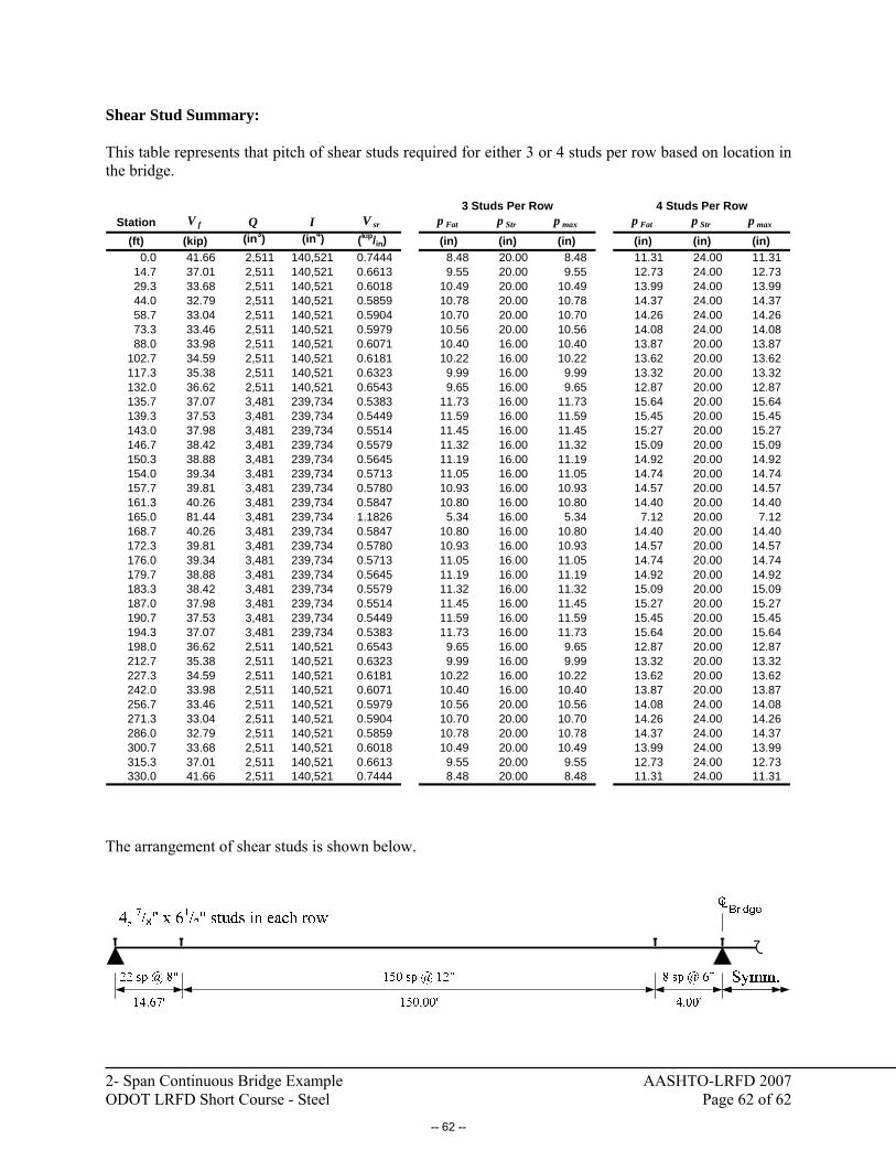
2- Span Continuous Bridge Example AASHTO-LRFD 2007 ODOT LRFD Short Course - Steel Page 62 of 62
Shear Stud Summary: This table represents that pitch of shear studs required for either 3 or 4 studs per row based on location in the bridge.
Station V f Q I V sr p Fat p Str p max p Fat p Str p max
(ft) (kip) (in3) (in4) (kip/in) (in) (in) (in) (in) (in) (in)0.0 41.66 2,511 140,521 0.7444 8.48 20.00 8.48 11.31 24.00 11.31
14.7 37.01 2,511 140,521 0.6613 9.55 20.00 9.55 12.73 24.00 12.7329.3 33.68 2,511 140,521 0.6018 10.49 20.00 10.49 13.99 24.00 13.9944.0 32.79 2,511 140,521 0.5859 10.78 20.00 10.78 14.37 24.00 14.3758.7 33.04 2,511 140,521 0.5904 10.70 20.00 10.70 14.26 24.00 14.2673.3 33.46 2,511 140,521 0.5979 10.56 20.00 10.56 14.08 24.00 14.0888.0 33.98 2,511 140,521 0.6071 10.40 16.00 10.40 13.87 20.00 13.87
102.7 34.59 2,511 140,521 0.6181 10.22 16.00 10.22 13.62 20.00 13.62117.3 35.38 2,511 140,521 0.6323 9.99 16.00 9.99 13.32 20.00 13.32132.0 36.62 2,511 140,521 0.6543 9.65 16.00 9.65 12.87 20.00 12.87135.7 37.07 3,481 239,734 0.5383 11.73 16.00 11.73 15.64 20.00 15.64139.3 37.53 3,481 239,734 0.5449 11.59 16.00 11.59 15.45 20.00 15.45143.0 37.98 3,481 239,734 0.5514 11.45 16.00 11.45 15.27 20.00 15.27146.7 38.42 3,481 239,734 0.5579 11.32 16.00 11.32 15.09 20.00 15.09150.3 38.88 3,481 239,734 0.5645 11.19 16.00 11.19 14.92 20.00 14.92154.0 39.34 3,481 239,734 0.5713 11.05 16.00 11.05 14.74 20.00 14.74157.7 39.81 3,481 239,734 0.5780 10.93 16.00 10.93 14.57 20.00 14.57161.3 40.26 3,481 239,734 0.5847 10.80 16.00 10.80 14.40 20.00 14.40165.0 81.44 3,481 239,734 1.1826 5.34 16.00 5.34 7.12 20.00 7.12168.7 40.26 3,481 239,734 0.5847 10.80 16.00 10.80 14.40 20.00 14.40172.3 39.81 3,481 239,734 0.5780 10.93 16.00 10.93 14.57 20.00 14.57176.0 39.34 3,481 239,734 0.5713 11.05 16.00 11.05 14.74 20.00 14.74179.7 38.88 3,481 239,734 0.5645 11.19 16.00 11.19 14.92 20.00 14.92183.3 38.42 3,481 239,734 0.5579 11.32 16.00 11.32 15.09 20.00 15.09187.0 37.98 3,481 239,734 0.5514 11.45 16.00 11.45 15.27 20.00 15.27190.7 37.53 3,481 239,734 0.5449 11.59 16.00 11.59 15.45 20.00 15.45194.3 37.07 3,481 239,734 0.5383 11.73 16.00 11.73 15.64 20.00 15.64198.0 36.62 2,511 140,521 0.6543 9.65 16.00 9.65 12.87 20.00 12.87212.7 35.38 2,511 140,521 0.6323 9.99 16.00 9.99 13.32 20.00 13.32227.3 34.59 2,511 140,521 0.6181 10.22 16.00 10.22 13.62 20.00 13.62242.0 33.98 2,511 140,521 0.6071 10.40 16.00 10.40 13.87 20.00 13.87256.7 33.46 2,511 140,521 0.5979 10.56 20.00 10.56 14.08 24.00 14.08271.3 33.04 2,511 140,521 0.5904 10.70 20.00 10.70 14.26 24.00 14.26286.0 32.79 2,511 140,521 0.5859 10.78 20.00 10.78 14.37 24.00 14.37300.7 33.68 2,511 140,521 0.6018 10.49 20.00 10.49 13.99 24.00 13.99315.3 37.01 2,511 140,521 0.6613 9.55 20.00 9.55 12.73 24.00 12.73330.0 41.66 2,511 140,521 0.7444 8.48 20.00 8.48 11.31 24.00 11.31
3 Studs Per Row 4 Studs Per Row
The arrangement of shear studs is shown below.
-- 62 --
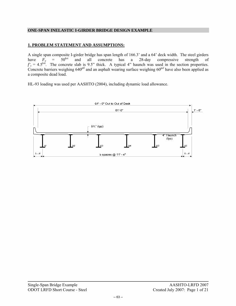
Single-Span Bridge Example AASHTO-LRFD 2007 ODOT LRFD Short Course - Steel Created July 2007: Page 1 of 21
ONE-SPAN INELASTIC I-GIRDER BRIDGE DESIGN EXAMPLE 1. PROBLEM STATEMENT AND ASSUMPTIONS: A single span composite I-girder bridge has span length of 166.3’ and a 64’ deck width. The steel girders have Fy = 50ksi and all concrete has a 28-day compressive strength of f’c = 4.5ksi. The concrete slab is 9.5” thick. A typical 4” haunch was used in the section properties. Concrete barriers weighing 640plf and an asphalt wearing surface weighing 60psf have also been applied as a composite dead load. HL-93 loading was used per AASHTO (2004), including dynamic load allowance.
-- 63 --
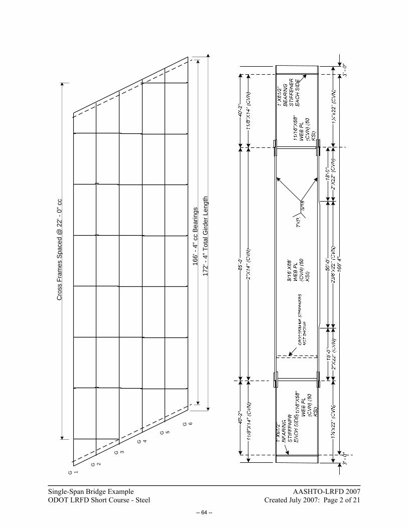
Single-Span Bridge Example AASHTO-LRFD 2007 ODOT LRFD Short Course - Steel Created July 2007: Page 2 of 21
166'
-4"
cc
Bea
rings
172'
-4"
Tot
al G
irder
Len
gth
G 1
G 2
G 3
G 4
G 5
G 6
Cro
ss F
ram
es S
pace
d @
22'
-0"
cc
-- 64 --
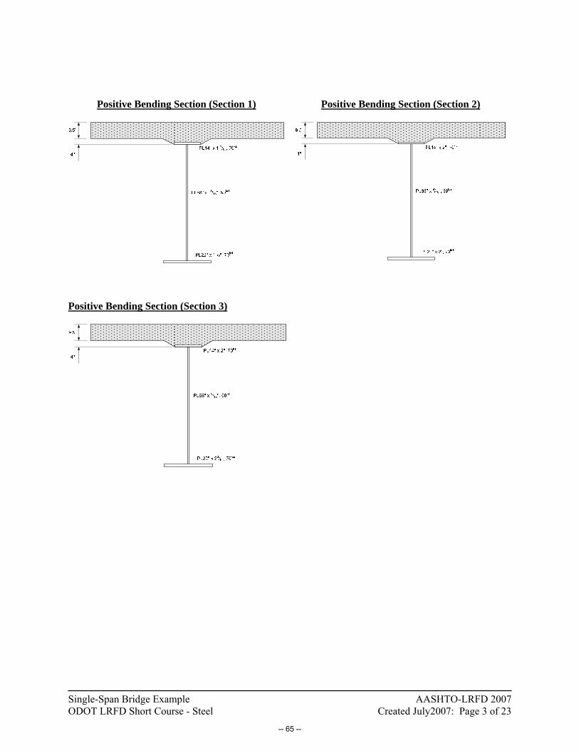
Single-Span Bridge Example AASHTO-LRFD 2007 ODOT LRFD Short Course - Steel Created July2007: Page 3 of 23
Positive Bending Section (Section 1)
Positive Bending Section (Section 2)
Positive Bending Section (Section 3)
-- 65 --
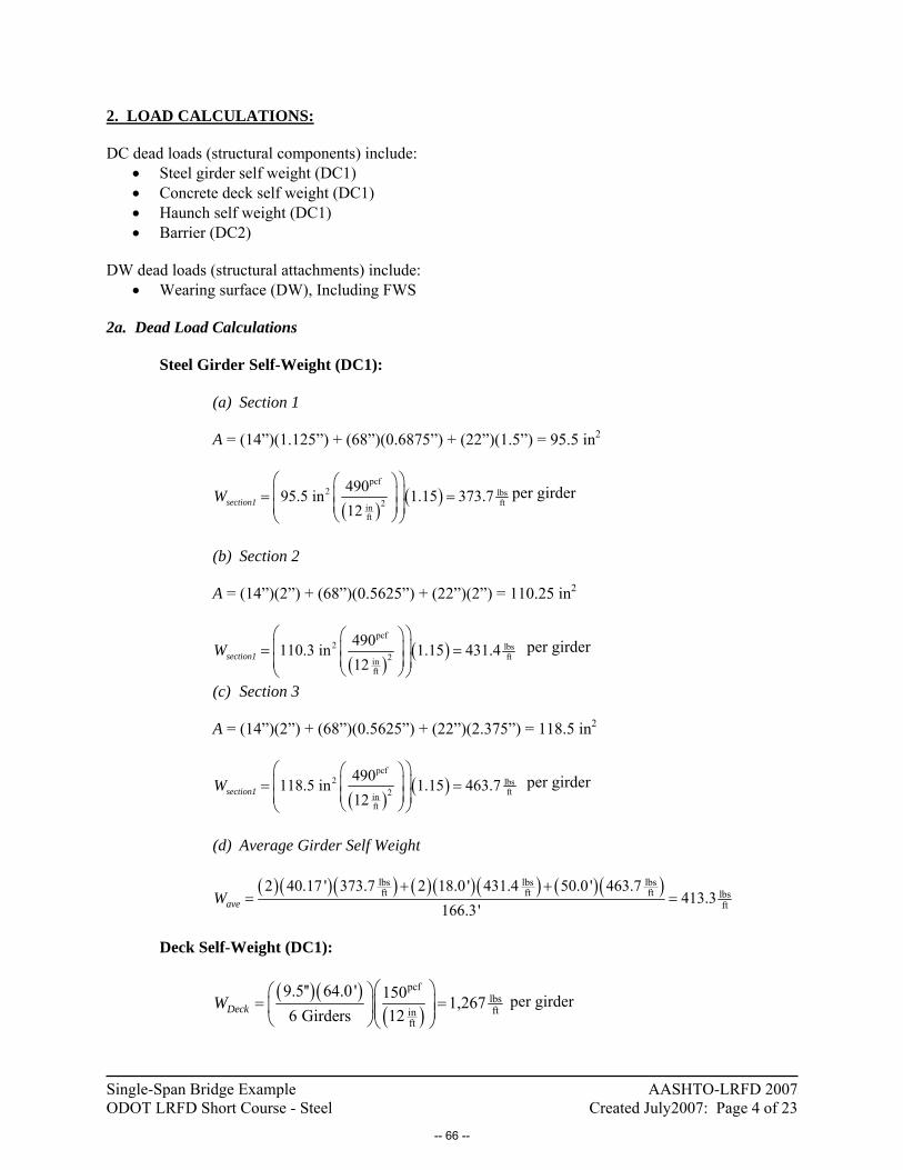
Single-Span Bridge Example AASHTO-LRFD 2007 ODOT LRFD Short Course - Steel Created July2007: Page 4 of 23
2. LOAD CALCULATIONS: DC dead loads (structural components) include:
• Steel girder self weight (DC1) • Concrete deck self weight (DC1) • Haunch self weight (DC1) • Barrier (DC2)
DW dead loads (structural attachments) include:
• Wearing surface (DW), Including FWS 2a. Dead Load Calculations
Steel Girder Self-Weight (DC1):
(a) Section 1
A = (14”)(1.125”) + (68”)(0.6875”) + (22”)(1.5”) = 95.5 in2
( )( )
pcf2 lbs
ft2inft
49095.5 in 1.15 373.712
section1W⎛ ⎞⎛ ⎞⎜ ⎟⎜ ⎟= =
⎜ ⎟⎜ ⎟⎝ ⎠⎝ ⎠
per girder
(b) Section 2 A = (14”)(2”) + (68”)(0.5625”) + (22”)(2”) = 110.25 in2
( )( )
pcf2 lbs
ft2inft
490110.3 in 1.15 431.412
section1W⎛ ⎞⎛ ⎞⎜ ⎟⎜ ⎟= =
⎜ ⎟⎜ ⎟⎝ ⎠⎝ ⎠
per girder
(c) Section 3 A = (14”)(2”) + (68”)(0.5625”) + (22”)(2.375”) = 118.5 in2
( )( )
pcf2 lbs
ft2inft
490118.5 in 1.15 463.712
section1W⎛ ⎞⎛ ⎞⎜ ⎟⎜ ⎟= =
⎜ ⎟⎜ ⎟⎝ ⎠⎝ ⎠
per girder
(d) Average Girder Self Weight
( )( )( ) ( )( )( ) ( )( )lbs lbs lbsft ft ft lbs
ft
2 40.17 ' 373.7 2 18.0 ' 431.4 50.0 ' 463.7413.3
166.3'aveW+ +
= =
Deck Self-Weight (DC1):
( )( )( )
pcflbsftin
ft
9.5'' 64.0 ' 150 1,2676 Girders 12DeckW
⎛ ⎞⎛ ⎞= =⎜ ⎟⎜ ⎟⎜ ⎟⎝ ⎠⎝ ⎠
per girder
-- 66 --
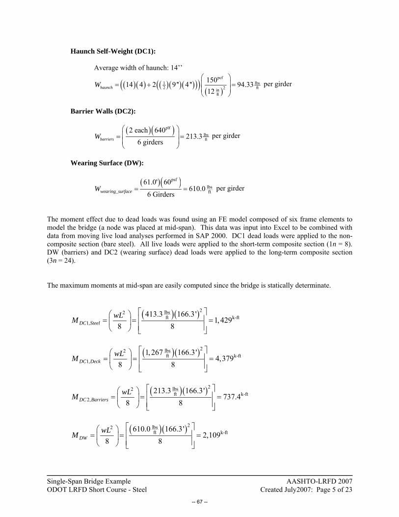
Single-Span Bridge Example AASHTO-LRFD 2007 ODOT LRFD Short Course - Steel Created July2007: Page 5 of 23
Haunch Self-Weight (DC1):
Average width of haunch: 14’’
( )( ) ( )( )( )( )( )( )
pcflbs1
2 ft2inft
15014 4 2 9 '' 4 '' 94.3312
haunchW⎛ ⎞⎜ ⎟= + =⎜ ⎟⎝ ⎠
per girder
Barrier Walls (DC2):
( )( )plflbsft
2 each 640213.3
6 girdersbarriersW⎛ ⎞⎜ ⎟= =⎜ ⎟⎝ ⎠
per girder
Wearing Surface (DW):
( )( )psflbsft
61.0' 60610.0
6 Girderswearing_surfaceW = = per girder
The moment effect due to dead loads was found using an FE model composed of six frame elements to model the bridge (a node was placed at mid-span). This data was input into Excel to be combined with data from moving live load analyses performed in SAP 2000. DC1 dead loads were applied to the non-composite section (bare steel). All live loads were applied to the short-term composite section (1n = 8). DW (barriers) and DC2 (wearing surface) dead loads were applied to the long-term composite section (3n = 24). The maximum moments at mid-span are easily computed since the bridge is statically determinate.
( )( )2lbs2
ft k-ft1,
413.3 166.3'1, 429
8 8DC SteelwLM
⎡ ⎤⎛ ⎞⎢ ⎥= = =⎜ ⎟⎢ ⎥⎝ ⎠ ⎣ ⎦
( )( )2lbs2ft k-ft
1,1, 267 166.3'
4,3798 8DC Deck
wLM⎡ ⎤⎛ ⎞⎢ ⎥= = =⎜ ⎟⎢ ⎥⎝ ⎠ ⎣ ⎦
( )( )2lbs2ft k-ft
2,213.3 166.3'
737.48 8DC Barriers
wLM⎡ ⎤⎛ ⎞⎢ ⎥= = =⎜ ⎟⎢ ⎥⎝ ⎠ ⎣ ⎦
( )( )2lbs2ft k-ft610.0 166.3'
2,1098 8DW
wLM⎡ ⎤⎛ ⎞⎢ ⎥= = =⎜ ⎟⎢ ⎥⎝ ⎠ ⎣ ⎦
-- 67 --
Single-Span Bridge Example AASHTO-LRFD 2007 ODOT LRFD Short Course - Steel Created July2007: Page 6 of 23
The maximum shear forces at the ends of the girder are also easily computed.
( )( )lbsft kip
1,413.3 166.3'
34.372 2DC Steel
wLV⎡ ⎤⎛ ⎞= = =⎢ ⎥⎜ ⎟
⎝ ⎠ ⎢ ⎥⎣ ⎦
( )( )lbsft kipt
1,1, 267 166.3'
105.42 2DC Deck
wLV⎡ ⎤⎛ ⎞= = =⎢ ⎥⎜ ⎟
⎝ ⎠ ⎢ ⎥⎣ ⎦
( )( )lbsft kip
2,213.3 166.3'
17.742 2DC Barriers
wLV⎡ ⎤⎛ ⎞= = =⎢ ⎥⎜ ⎟
⎝ ⎠ ⎢ ⎥⎣ ⎦
( )( )lbsft kip610.0 166.3'
50.722 2DW
wLV⎡ ⎤⎛ ⎞= = =⎢ ⎥⎜ ⎟
⎝ ⎠ ⎢ ⎥⎣ ⎦
-- 68 --
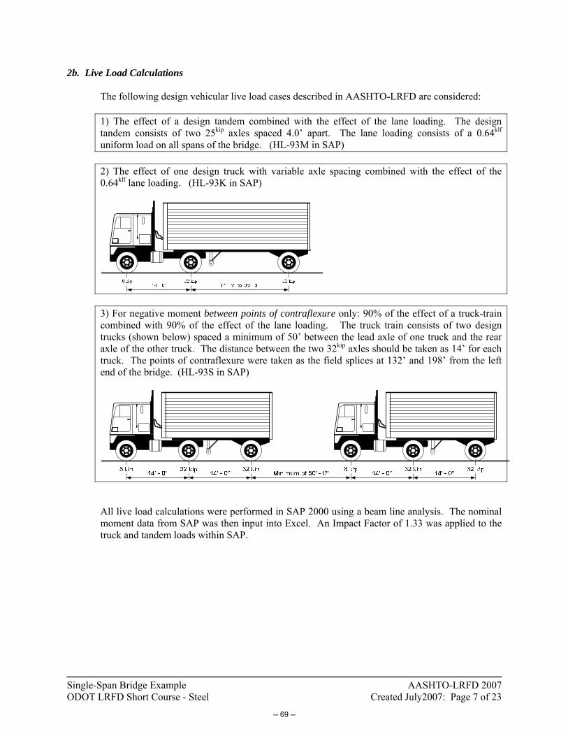
Single-Span Bridge Example AASHTO-LRFD 2007 ODOT LRFD Short Course - Steel Created July2007: Page 7 of 23
2b. Live Load Calculations
The following design vehicular live load cases described in AASHTO-LRFD are considered: 1) The effect of a design tandem combined with the effect of the lane loading. The design tandem consists of two 25kip axles spaced 4.0’ apart. The lane loading consists of a 0.64klf uniform load on all spans of the bridge. (HL-93M in SAP) 2) The effect of one design truck with variable axle spacing combined with the effect of the 0.64klf lane loading. (HL-93K in SAP)
3) For negative moment between points of contraflexure only: 90% of the effect of a truck-train combined with 90% of the effect of the lane loading. The truck train consists of two design trucks (shown below) spaced a minimum of 50’ between the lead axle of one truck and the rear axle of the other truck. The distance between the two 32kip axles should be taken as 14’ for each truck. The points of contraflexure were taken as the field splices at 132’ and 198’ from the left end of the bridge. (HL-93S in SAP)
All live load calculations were performed in SAP 2000 using a beam line analysis. The nominal moment data from SAP was then input into Excel. An Impact Factor of 1.33 was applied to the truck and tandem loads within SAP.
-- 69 --

Single-Span Bridge Example AASHTO-LRFD 2007 ODOT LRFD Short Course - Steel Created July2007: Page 8 of 23
Unfactored HL-93 Moment Envelopes from SAP
-6,000
-4,000
-2,000
0
2,000
4,000
6,000
0 30 60 90 120 150
Station (ft)
Mom
ent (
kip-
ft)
Single Truck
Tandem
The following results were obtained from the SAP analysis:
• The maximum positive live-load moments occur at stations 83.15’
Station 40.16’- Section 1 Station 58.15’- Section 2 Station 83.15’- Section 3 HL-93M 3,614k-ft 4,481k-ft 4,911k-ft HL-93K 4,322k-ft 5,238k-ft 5,821k-ft HL-93S N/A N/A N/A
Before proceeding, these live-load moments will be confirmed with an influence line analysis.
-- 70 --

Single-Span Bridge Example AASHTO-LRFD 2007 ODOT LRFD Short Course - Steel Created July2007: Page 9 of 23
2c. Verify the Maximum Positive Live-Load Moment at Station 83.15’:
Tandem: ( )( ) ( )( )kip kip k-ftk-ft k-ft
kip kip25 41.58 25 39.58 2,029+ =
Single Truck: ( )( ) ( )( ) ( )( )kip kip kip k-ftk-ft k-ft k-ftkip kip kip8 34.57 32 41.58 32 34.57 2,713+ + =
Lane Load: ( )( ) k-ftk-ft k-ftkip kip0.640 3, 457 2, 212=
(IM)(Tandem) + Lane: ( )( ) k-ft k-ftk-ftkip1.33 2, 029 2, 212 4,911+ =
(IM)(Single Truck) + Lane: ( )( ) k-ft k-ftk-ftkip1.33 2,713 2, 212 5,821+ = GOVERNS
The case of two trucks is not considered here because it is only used when computing negative moments.
Single Truck
Tandem :
Lane
8kip
32kip 32kip
25kip25kip
0.640kip/ft
:
05
1015202530354045
0 15 30 45 60 75 90 105 120 135 150 165
Station (ft)
Mom
ent (
k-ft
/ kip
)
-- 71 --

Single-Span Bridge Example AASHTO-LRFD 2007 ODOT LRFD Short Course - Steel Created July2007: Page 10 of 23
Based on the influence line analysis, we can say that the moments obtained from SAP appear to be reasonable and will be used for design.
Before these Service moments can be factored and combined, we must compute the distribution factors. Since the distribution factors are a function of Kg, the longitudinal stiffness parameter, we must first compute the sections properties of the girders. 3. SECTION PROPERTIES AND CALCULATIONS: 3a. Effective Flange Width, bs:
For an interior beam, bs is the lesser of:
( )( )
( )( )inft
14"12 12 8.5" 109 ''2 2
11.33' 12 135.96 ''
166.3' 41.58' 498.9 ''4 4
fs
eff
bt
SL
⎧• + = + =⎪⎪⎪• = =⎨⎪⎪• = = =⎪⎩
Therefore, bs = 109”
For computing the section properties shown on the two pages that follow, reinforcing steel in the deck was ignored for short-term and long-term composite calculations but was included for the cracked section. Note: At this point one should also check the effective of the outside girders as well. For this example, however, I will proceed sing the effective width for the interior girders.
-- 72 --

Single-Span Bridge Example AASHTO-LRFD 2007 ODOT LRFD Short Course - Steel Created July2007: Page 11 of 23
3b. Section 1 Flexural Properties
Bare Steel
t b A y Ay Ix d Ad2 IXTop Flange 1.1250 14.00 15.75 70.06 1,103.48 1.66 -40.87 26,308 26,310Web 0.6875 68.00 46.75 35.50 1,659.63 18,014.33 -6.31 1,860 19,874Bot Flange 1.5000 22.00 33.00 0.75 24.75 6.19 28.44 26,696 26,702
95.50 2,787.86 ITotal = 72,886
Y = 29.19 SBS1,top = 1,759SBS1,bot = 2,497
Short-Term Composite (N=8)
t b A y Ay Ix d Ad2 IX
Slab 8.5000 109.00 115.81 74.88 8,671.46 697.29 -20.65 49,365 50,062Haunch 0.0000 14.0000 0.00 70.63 0.00 0.00 -16.40 0 0Top Flange 1.1250 14.0000 15.75 70.06 1,103.48 1.66 -15.83 3,948 3,950Web 0.6875 68.0000 46.75 35.50 1,659.63 18,014.33 18.73 16,399 34,414Bot Flange 1.5000 22.0000 33.00 0.75 24.75 6.19 53.48 94,381 94,387
211.31 11,459.32 ITotal = 182,813
n = 8.00 Y = 54.23 SST1,top = 11,150SST1,bot = 3,371
Long-Term Composite (N=24)
t b A y Ay Ix d Ad2 IXSlab 8.5000 109.00 38.60 74.88 2,890.49 232.43 -32.53 40,856 41,089Haunch 0.0000 14.00 0.00 70.63 0.00 0.00 -28.28 0 0Top Flange 1.1250 14.0000 15.75 70.06 1,103.48 1.66 -27.72 12,102 12,104Web 0.6875 68.0000 46.75 35.50 1,659.63 18,014.33 6.84 2,189 20,203Bot Flange 1.5000 22.0000 33.00 0.75 24.75 6.19 41.59 57,089 57,095
134.10 5,678.35 ITotal = 130,491
n = 24.00 Y = 42.34 SLT1,top = 4,614SLT1,bot = 3,082
Single Span Bridge Example - Section 1
-- 73 --

Single-Span Bridge Example AASHTO-LRFD 2007 ODOT LRFD Short Course - Steel Created July2007: Page 12 of 23
3c. Section 2 Flexural Properties
Bare Steel
t b A y Ay Ix d Ad2 IXTop Flange 2.0000 14.00 28.00 71.00 1,988.00 9.33 -40.08 44,978 44,987Web 0.5625 68.00 38.25 36.00 1,377.00 14,739.00 -5.08 987 15,726Bot Flange 2.0000 22.00 44.00 1.00 44.00 14.67 29.92 39,391 39,405
110.25 3,409.00 ITotal = 100,119
Y = 30.92 SBS1,top = 2,437SBS1,bot = 3,238
Short-Term Composite (N=8)
t b A y Ay Ix d Ad2 IXSlab 8.5000 109.00 115.81 76.25 8,830.70 697.29 -22.11 56,600 57,297Haunch 0.0000 14.0000 0.00 72.00 0.00 0.00 -17.86 0 0Top Flange 2.0000 14.0000 28.00 71.00 1,988.00 9.33 -16.86 7,956 7,966Web 0.5625 68.0000 38.25 36.00 1,377.00 14,739.00 18.14 12,591 27,330Bot Flange 2.0000 22.0000 44.00 1.00 44.00 14.67 53.14 124,264 124,279
226.06 12,239.70 ITotal = 216,871
n = 8.00 Y = 54.14 SST1,top = 12,145SST1,bot = 4,006
Long-Term Composite (N=24)
t b A y Ay Ix d Ad2 IXSlab 8.5000 109.00 38.60 76.25 2,943.57 232.43 -33.57 43,514 43,746Haunch 0.0000 14.00 0.00 72.00 0.00 0.00 -29.32 0 0Top Flange 2.0000 14.0000 28.00 71.00 1,988.00 9.33 -28.32 22,462 22,472Web 0.5625 68.0000 38.25 36.00 1,377.00 14,739.00 6.68 1,705 16,444Bot Flange 2.0000 22.0000 44.00 1.00 44.00 14.67 41.68 76,425 76,439
148.85 6,352.57 ITotal = 159,101
n = 24.00 Y = 42.68 SLT1,top = 5,426SLT1,bot = 3,728
Single Span Bridge Example - Section 2
-- 74 --

Single-Span Bridge Example AASHTO-LRFD 2007 ODOT LRFD Short Course - Steel Created July2007: Page 13 of 23
3d. Section 3 Flexural Properties
Bare Steel
t b A y Ay Ix d Ad2 IXTop Flange 2.0000 14.00 28.00 71.38 1,998.50 9.33 -42.25 49,970 49,980Web 0.5625 68.00 38.25 36.38 1,391.34 14,739.00 -7.25 2,008 16,747Bot Flange 2.3750 22.00 52.25 1.19 62.05 24.56 27.94 40,796 40,820
118.50 3,451.89 ITotal = 107,546
Y = 29.13 SBS1,top = 2,487SBS1,bot = 3,692
Short-Term Composite (N=8)
t b A y Ay Ix d Ad2 IXSlab 8.5000 109.00 115.81 76.63 8,874.13 697.29 -24.02 66,819 67,516Haunch 0.0000 14.0000 0.00 72.38 0.00 0.00 -19.77 0 0Top Flange 2.0000 14.0000 28.00 71.38 1,998.50 9.33 -18.77 9,865 9,874Web 0.5625 68.0000 38.25 36.38 1,391.34 14,739.00 16.23 10,076 24,815Bot Flange 2.3750 22.0000 52.25 1.19 62.05 24.56 51.42 138,137 138,161
234.31 12,326.02 ITotal = 240,366
n = 8.00 Y = 52.61 SST1,top = 12,158SST1,bot = 4,569
Long-Term Composite (N=24)
t b A y Ay Ix d Ad2 IXSlab 8.5000 109.00 38.60 76.63 2,958.04 232.43 -35.82 49,544 49,777Haunch 0.0000 14.00 0.00 72.38 0.00 0.00 -31.57 0 0Top Flange 2.0000 14.0000 28.00 71.38 1,998.50 9.33 -30.57 26,174 26,184Web 0.5625 68.0000 38.25 36.38 1,391.34 14,739.00 4.43 749 15,488Bot Flange 2.3750 22.0000 52.25 1.19 62.05 24.56 39.61 81,990 82,015
157.10 6,409.93 ITotal = 173,463
n = 24.00 Y = 40.80 SLT1,top = 5,494SLT1,bot = 4,251
Single Span Bridge Example - Section 3
-- 75 --

Single-Span Bridge Example AASHTO-LRFD 2007 ODOT LRFD Short Course - Steel Created July2007: Page 14 of 23
4. DISTRIBUTION FACTOR FOR MOMENT 4a. Section 1:
Interior Girder - One Lane Loaded:
( )( )( )( )
( )( )( )
0.10.4 0.3
3
2
24 2
4
0.4 0.3 4
3
0.0614 12
(8) 72,890 in 95.5 in 49.06"
2,422,000 in
11.33' 11.33' 2, 422,000 in0.0614 166.3' 12 166.3' 8.5"
gM1,Int,Sec1
S
g g
g
g
M1,Int,Sec1
KS SDFL Lt
K n I Ae
K
K
DF
⎛ ⎞⎛ ⎞ ⎛ ⎞= + ⎜ ⎟⎜ ⎟ ⎜ ⎟⎝ ⎠ ⎝ ⎠ ⎝ ⎠
= +
= +
=
⎛ ⎞ ⎛ ⎞= + ⎜ ⎟ ⎜ ⎟⎝ ⎠ ⎝ ⎠
0.1
0.4994M1,Int,Sec1DF
⎛ ⎞⎜ ⎟⎜ ⎟⎝ ⎠
=
Interior Girder - Two or More Lanes Loaded:
( )( )( )
0.10.4 0.3
3
0.10.6 0.2 4
3
0.0759.5 12
11.33' 11.33' 2, 422,000 in0.0759.5 166.3' 12 166.3' 8.5"
0.7703
gM2,Int,Sec1
S
M2,Int,Sec1
M2,Int,Sec1
KS SDFL Lt
DF
DF
⎛ ⎞⎛ ⎞ ⎛ ⎞= + ⎜ ⎟⎜ ⎟ ⎜ ⎟⎝ ⎠ ⎝ ⎠ ⎝ ⎠
⎛ ⎞⎛ ⎞ ⎛ ⎞= + ⎜ ⎟⎜ ⎟ ⎜ ⎟ ⎜ ⎟⎝ ⎠ ⎝ ⎠ ⎝ ⎠=
-- 76 --

Single-Span Bridge Example AASHTO-LRFD 2007 ODOT LRFD Short Course - Steel Created July2007: Page 15 of 23
Exterior Girder – One Lane Loaded:
The lever rule is applied by assuming that a hinge forms over the first interior girder as a truck load is applied near the parapet. The resulting reaction in the exterior girder is the distribution factor.
1 18 5' 0 7500
11 33'M ,Ext,Sec.DF ..
= =
Multiple Presence: DFM1,Ext,Sec1 = (1.2) (0.7500) = 0.9000
Exterior Girder - Two or More Lanes Loaded:
DFM2,Ext,Sec1 = e DFM2,Int,Sec1
0.77
9.12.167 '0.77 1.008
9.1
ede
e
= +
= + =
DFM2,Ext+ = (1.008) (0.7703) = 0.7765
4b. Section 2:
Interior Girder – One Lane Loaded:
( )( )( )( )
( )( )
0.10.4 0.3
3
2
24 2
4
0.4 0.3 4
0.0614 12
(8) 100,100 in 110.3 in 47.83"
2,819,000 in
11.33' 11.33' 2,819,000 in0.0614 166.3' 12 166.3' 8.5
gM1,Int,Sec2
S
g g
g
g
M1,Int,Sec2
KS SDFL Lt
K n I Ae
K
K
DF
⎛ ⎞⎛ ⎞ ⎛ ⎞= + ⎜ ⎟⎜ ⎟ ⎜ ⎟⎝ ⎠ ⎝ ⎠ ⎝ ⎠
= +
= +
=
⎛ ⎞ ⎛ ⎞= + ⎜ ⎟ ⎜ ⎟⎝ ⎠ ⎝ ⎠ ( )
0.1
3"
0.5061M1,Int,Sec2DF
⎛ ⎞⎜ ⎟⎜ ⎟⎝ ⎠
=
-- 77 --
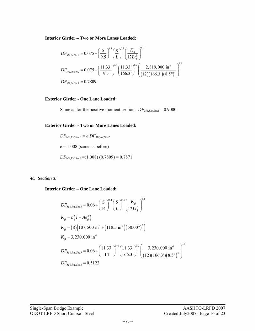
Single-Span Bridge Example AASHTO-LRFD 2007 ODOT LRFD Short Course - Steel Created July2007: Page 16 of 23
Interior Girder – Two or More Lanes Loaded:
( )( )( )
0.10.4 0.3
3
0.10.6 0.2 4
3
0.0759.5 12
11.33' 11.33' 2,819,000 in0.0759.5 166.3' 12 166.3' 8.5"
0.7809
gM2,Int,Sec2
S
M2,Int,Sec2
M2,Int,Sec2
KS SDFL Lt
DF
DF
⎛ ⎞⎛ ⎞ ⎛ ⎞= + ⎜ ⎟⎜ ⎟ ⎜ ⎟⎝ ⎠ ⎝ ⎠ ⎝ ⎠
⎛ ⎞⎛ ⎞ ⎛ ⎞= + ⎜ ⎟⎜ ⎟ ⎜ ⎟ ⎜ ⎟⎝ ⎠ ⎝ ⎠ ⎝ ⎠=
Exterior Girder - One Lane Loaded:
Same as for the positive moment section: DFM1,Ext,Sec2 = 0.9000
Exterior Girder - Two or More Lanes Loaded:
DFM2,Ext,Sec2 = e DFM2,Int,Sec2
e = 1.008 (same as before)
DFM2,Ext,Sec2 =(1.008) (0.7809) = 0.7871
4c. Section 3:
Interior Girder – One Lane Loaded:
( )( ) ( )( )( )
( ) ( )( )
0.10.4 0.3
1, , 3 3
2
24 2
4
0.4 0.3 4
1, , 3 3
0.0614 12
8 107,500 in 118.5 in 50.00"
3, 230,000 in
11.33' 11.33' 3, 230,000 in0.0614 166.3' 12 166.3' 8.5"
gM Int Sec
S
g g
g
g
M Int Sec
KS SDFL Lt
K n I Ae
K
K
DF
⎛ ⎞⎛ ⎞ ⎛ ⎞= + ⎜ ⎟⎜ ⎟ ⎜ ⎟⎝ ⎠ ⎝ ⎠ ⎝ ⎠
= +
= +
=
⎛ ⎞ ⎛ ⎞= + ⎜ ⎟ ⎜ ⎟⎝ ⎠ ⎝ ⎠
0.1
1, , 3 0.5122M Int SecDF
⎛ ⎞⎜ ⎟⎜ ⎟⎝ ⎠
=
-- 78 --

Single-Span Bridge Example AASHTO-LRFD 2007 ODOT LRFD Short Course - Steel Created July2007: Page 17 of 23
Interior Girder - Two or More Lanes Loaded:
( )( ) ( )
0.10.4 0.3
2, , 3 3
0.10.6 0.2 4
2, , 3 3
2, , 3
0.0759.5 12
11.33' 11.33' 3,230,000 in0.0759.5 166.3' 12 166.3' 8.5"
0.7906
gM Int Sec
S
M Int Sec
M Int Sec
KS SDFL Lt
DF
DF
⎛ ⎞⎛ ⎞ ⎛ ⎞= + ⎜ ⎟⎜ ⎟ ⎜ ⎟⎝ ⎠ ⎝ ⎠ ⎝ ⎠
⎛ ⎞⎛ ⎞ ⎛ ⎞ ⎜ ⎟= + ⎜ ⎟ ⎜ ⎟ ⎜ ⎟⎝ ⎠ ⎝ ⎠ ⎝ ⎠=
Exterior Girder – One Lane Loaded:
Same as for the positive moment section: DFM1,Ext,Sec3 = 0.9000
Exterior Girder - Two or More Lanes Loaded:
DFM2,Ext,Sec3 = e DFM2,Int,Sec3
e = 1.008 (same as before)
DFM2,Ext,Sec3 =(1.008) (0.7906) = 0.7969 4d. Minimum Exterior Girder Distribution Factor:
,
2
L
Ext Minb
N
ExtL
Nb
X eN
DFN x
= +∑
∑
-- 79 --
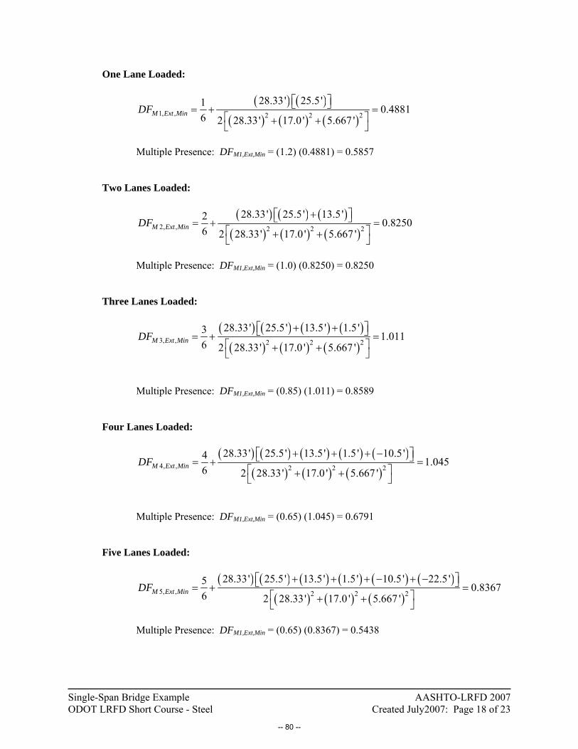
Single-Span Bridge Example AASHTO-LRFD 2007 ODOT LRFD Short Course - Steel Created July2007: Page 18 of 23
One Lane Loaded:
( ) ( )( ) ( ) ( )
1, , 2 2 2
28.33' 25.5 '1 0.48816 2 28.33' 17.0 ' 5.667 '
M Ext MinDF⎡ ⎤⎣ ⎦= + =
⎡ ⎤+ +⎣ ⎦
Multiple Presence: DFM1,Ext,Min = (1.2) (0.4881) = 0.5857
Two Lanes Loaded:
( ) ( ) ( )
( ) ( ) ( )2, , 2 2 2
28.33' 25.5 ' 13.5 '2 0.82506 2 28.33' 17.0 ' 5.667 '
M Ext MinDF+⎡ ⎤⎣ ⎦= + =
⎡ ⎤+ +⎣ ⎦
Multiple Presence: DFM1,Ext,Min = (1.0) (0.8250) = 0.8250
Three Lanes Loaded:
( ) ( ) ( ) ( )( ) ( ) ( )
3, , 2 2 2
28.33' 25.5 ' 13.5 ' 1.5 '3 1.0116 2 28.33' 17.0 ' 5.667 '
M Ext MinDF+ +⎡ ⎤⎣ ⎦= + =
⎡ ⎤+ +⎣ ⎦
Multiple Presence: DFM1,Ext,Min = (0.85) (1.011) = 0.8589
Four Lanes Loaded:
( ) ( ) ( ) ( ) ( )
( ) ( ) ( )4, , 2 2 2
28.33' 25.5 ' 13.5 ' 1.5 ' 10.5 '4 1.0456 2 28.33' 17.0 ' 5.667 '
M Ext MinDF+ + + −⎡ ⎤⎣ ⎦= + =
⎡ ⎤+ +⎣ ⎦
Multiple Presence: DFM1,Ext,Min = (0.65) (1.045) = 0.6791
Five Lanes Loaded:
( ) ( ) ( ) ( ) ( ) ( )
( ) ( ) ( )5, , 2 2 2
28.33' 25.5 ' 13.5 ' 1.5 ' 10.5 ' 22.5 '5 0.83676 2 28.33' 17.0 ' 5.667 '
M Ext MinDF+ + + − + −⎡ ⎤⎣ ⎦= + =
⎡ ⎤+ +⎣ ⎦
Multiple Presence: DFM1,Ext,Min = (0.65) (0.8367) = 0.5438
-- 80 --

Single-Span Bridge Example AASHTO-LRFD 2007 ODOT LRFD Short Course - Steel Created July2007: Page 19 of 23
4d. Moment Distribution Factor Summary
Positive Moment Section # Lanes Loaded Interior Exterior
1 0.4994 0.9000 ≥ 0.5857 2 0.7703 0.7765 ≥ 0.8250 1 3 0.7703 0.7765 ≥ 0.8589 1 0.5061 0.9000 ≥ 0.5857 2 0.7809 0.7871 ≥ 0.8250 2 3 0.7809 0.7871 ≥ 0.8589 1 0.5122 0.9000 ≥ 0.5857 2 0.7906 0.7969 ≥ 0.8250 3 3 0.7906 0.7969 ≥ 0.8589
For Simplicity, take the Moment Distribution Factor as 0.9000 everywhere. Multiplying the live load moments by this distribution factor of 0.9000 yields the table of “nominal” girder moments shown below.
Nominal Girder Moments from Visual Analysis and SAP
Station LL+ LL- DC1 DC2 DW(ft) (k-ft) (k-ft) (k-ft) (k-ft) (k-ft)
0.0 0.0 0.0 0.0 0.0 0.08.0 986.5 0.0 1086.2 135.6 457.7
16.1 1868.0 0.0 2064.8 257.4 869.024.1 2645.5 0.0 2935.8 365.5 1233.732.1 3319.1 0.0 3699.2 459.8 1552.040.2 3889.3 0.0 4355.1 540.3 1823.949.2 4404.3 0.0 4959.7 614.2 2073.358.2 4795.1 0.0 5424.7 670.8 2264.366.5 5054.9 0.0 5729.3 707.8 2389.174.8 5202.6 0.0 5912.1 730.0 2464.083.1 5238.6 0.0 5973.0 737.4 2489.083.1 5238.5 0.0 5973.0 737.4 2489.091.5 5202.6 0.0 5911.6 729.9 2463.899.8 5055.0 0.0 5728.3 707.7 2388.7
108.1 4795.7 0.0 5423.3 670.6 2263.7108.1 4795.2 0.0 5423.3 670.6 2263.7117.1 4404.5 0.0 4957.8 614.0 2072.4126.1 3890.2 0.0 4352.6 540.0 1822.9126.1 3889.5 0.0 4352.6 540.0 1822.9134.2 3319.4 0.0 3696.9 459.5 1551.1142.2 2645.7 0.0 2933.8 365.2 1232.9150.2 1868.1 0.0 2063.3 257.2 868.3158.3 986.6 0.0 1085.3 135.5 457.3166.3 1.1 0.0 0.0 0.0 0.0
Nominal Moments
-- 81 --
Single-Span Bridge Example AASHTO-LRFD 2007 ODOT LRFD Short Course - Steel Created July2007: Page 20 of 23
5. FACTORED MOMENT ENVELOPES
The following load combinations were considered in this example: Strength I: 1.75(LL + IM) + 1.25DC1 + 1.25DC2 + 1.50DW Strength IV: 1.50DC1 + 1.50DC2 + 1.50DW Service II: 1.3(LL + IM) + 1.0DC1 + 1.0DC2 + 1.0DW
Fatigue: 0.75(LL + IM) (IM for Fatigue = 15%) Strength II is not considered since this deals with special permit loads. Strength III and V are not considered as they include wind effects, which will be handled separately as needed. Strength IV is considered but is not expected to govern since it addresses situations with high dead load that come into play for longer spans. Extreme Event load combinations are not included as they are also beyond the scope of this example. Service I again applies to wind loads and is not considered and Service III and Service IV correspond to tension in prestressed concrete elements and are therefore not included in this example. In addition to the factors shown above, a load modifier, η, was applied as is shown below.
i i iQ Qη γ= ∑ η is taken as the product of ηD, ηR, and ηI, and is taken as not less than 0.95. For this example, ηD, ηR, and ηI are taken as 1.00. Using these load combinations, the shear and moment envelopes shown on the following pages were developed.
-- 82 --

Single-Span Bridge Example AASHTO-LRFD 2007 ODOT LRFD Short Course - Steel Created July2007: Page 21 of 23
Station LL+ LL- DC1 DC2 DW Total + Total -(ft) (k-ft) (k-ft) (k-ft) (k-ft) (k-ft) (k-ft) (k-ft)
0.0 0.0 0.0 0.0 0.0 0.0 0.0 0.08.0 1726.3 0.0 1357.7 169.5 686.6 3940.1 0.0
16.1 3268.9 0.0 2581.0 321.8 1303.4 7475.1 0.024.1 4629.6 0.0 3669.7 456.9 1850.6 10606.8 0.032.1 5808.5 0.0 4624.0 574.7 2328.1 13335.3 0.040.2 6806.2 0.0 5443.9 675.4 2735.8 15661.3 0.049.2 7707.5 0.0 6199.7 767.8 3109.9 17784.8 0.058.2 8391.4 0.0 6780.8 838.5 3396.5 19407.2 0.066.5 8846.1 0.0 7161.6 884.7 3583.7 20476.2 0.074.8 9104.5 0.0 7390.1 912.5 3696.0 21103.1 0.083.1 9167.5 0.0 7466.3 921.7 3733.5 21289.0 0.083.1 9167.4 0.0 7466.3 921.7 3733.5 21288.9 0.091.5 9104.6 0.0 7389.5 912.4 3695.7 21102.2 0.099.8 8846.3 0.0 7160.4 884.6 3583.1 20474.4 0.0
108.1 8392.4 0.0 6779.1 838.3 3395.6 19405.3 0.0108.1 8391.6 0.0 6779.1 838.3 3395.6 19404.5 0.0117.1 7707.8 0.0 6197.3 767.5 3108.7 17781.2 0.0126.1 6807.8 0.0 5440.8 675.0 2734.3 15657.9 0.0126.1 6806.6 0.0 5440.8 675.0 2734.3 15656.7 0.0134.2 5808.9 0.0 4621.1 574.4 2326.6 13331.0 0.0142.2 4630.0 0.0 3667.2 456.5 1849.3 10603.1 0.0150.2 3269.2 0.0 2579.1 321.5 1302.5 7472.2 0.0158.3 1726.5 0.0 1356.7 169.4 686.0 3938.5 0.0166.3 1.9 0.0 0.0 0.0 0.0 1.9 0.0
Strength I Moments
Station DC1 DC2 DW Total + Total -(ft) (k-ft) (k-ft) (k-ft) (k-ft) (k-ft)
0.0 0.0 0.0 0.0 0.0 0.07.2 1629.3 203.4 686.6 2519.2 0.0
14.5 3097.2 386.1 1303.4 4786.7 0.021.7 4403.7 548.2 1850.6 6802.5 0.028.9 5548.8 689.7 2328.1 8566.6 0.036.2 6532.6 810.5 2735.8 10078.9 0.043.4 7439.6 921.3 3109.9 11470.8 0.050.6 8137.0 1006.2 3396.5 12539.7 0.057.8 8593.9 1061.7 3583.7 13239.3 0.065.1 8868.1 1095.0 3696.0 13659.1 0.072.3 8959.5 1106.1 3733.5 13799.1 0.079.5 8959.5 1106.1 3733.5 13799.1 0.086.8 8867.4 1094.9 3695.7 13658.0 0.094.0 8592.5 1061.5 3583.1 13237.1 0.0
101.2 8134.9 1005.9 3395.6 12536.4 0.0108.5 8134.9 1005.9 3395.6 12536.4 0.0115.7 7436.7 920.9 3108.7 11466.3 0.0122.9 6529.0 810.0 2734.3 10073.3 0.0130.1 6529.0 810.0 2734.3 10073.3 0.0137.4 5545.4 689.3 2326.6 8561.2 0.0144.6 4400.7 547.9 1849.3 6797.8 0.0151.8 3094.9 385.9 1302.5 4783.2 0.0159.1 1628.0 203.2 686.0 2517.2 0.0166.3 0.0 0.0 0.0 0.0 0.0
Strength IV Moments
-- 83 --

Single-Span Bridge Example AASHTO-LRFD 2007 ODOT LRFD Short Course - Steel Created July2007: Page 22 of 23
Station LL+ LL- DC1 DC2 DW Total + Total -(ft) (k-ft) (k-ft) (k-ft) (k-ft) (k-ft) (k-ft) (k-ft)
0.0 0.0 0.0 0.0 0.0 0.0 0.0 0.07.2 1282.4 0.0 1086.2 135.6 457.7 2961.9 0.0
14.5 2428.3 0.0 2064.8 257.4 869.0 5619.5 0.021.7 3439.2 0.0 2935.8 365.5 1233.7 7974.2 0.028.9 4314.9 0.0 3699.2 459.8 1552.0 10026.0 0.036.2 5056.0 0.0 4355.1 540.3 1823.9 11775.3 0.043.4 5725.6 0.0 4959.7 614.2 2073.3 13372.8 0.050.6 6233.6 0.0 5424.7 670.8 2264.3 14593.4 0.057.8 6571.4 0.0 5729.3 707.8 2389.1 15397.6 0.065.1 6763.4 0.0 5912.1 730.0 2464.0 15869.4 0.072.3 6810.2 0.0 5973.0 737.4 2489.0 16009.6 0.079.5 6810.1 0.0 5973.0 737.4 2489.0 16009.5 0.086.8 6763.4 0.0 5911.6 729.9 2463.8 15868.7 0.094.0 6571.5 0.0 5728.3 707.7 2388.7 15396.3 0.0
101.2 6234.4 0.0 5423.3 670.6 2263.7 14591.9 0.0108.5 6233.8 0.0 5423.3 670.6 2263.7 14591.3 0.0115.7 5725.8 0.0 4957.8 614.0 2072.4 13370.0 0.0122.9 5057.2 0.0 4352.6 540.0 1822.9 11772.7 0.0130.1 5056.3 0.0 4352.6 540.0 1822.9 11771.8 0.0137.4 4315.2 0.0 3696.9 459.5 1551.1 10022.6 0.0144.6 3439.4 0.0 2933.8 365.2 1232.9 7971.3 0.0151.8 2428.5 0.0 2063.3 257.2 868.3 5617.3 0.0159.1 1282.5 0.0 1085.3 135.5 457.3 2960.7 0.0166.3 1.4 0.0 0.0 0.0 0.0 1.4 0.0
Service II Moments
-- 84 --
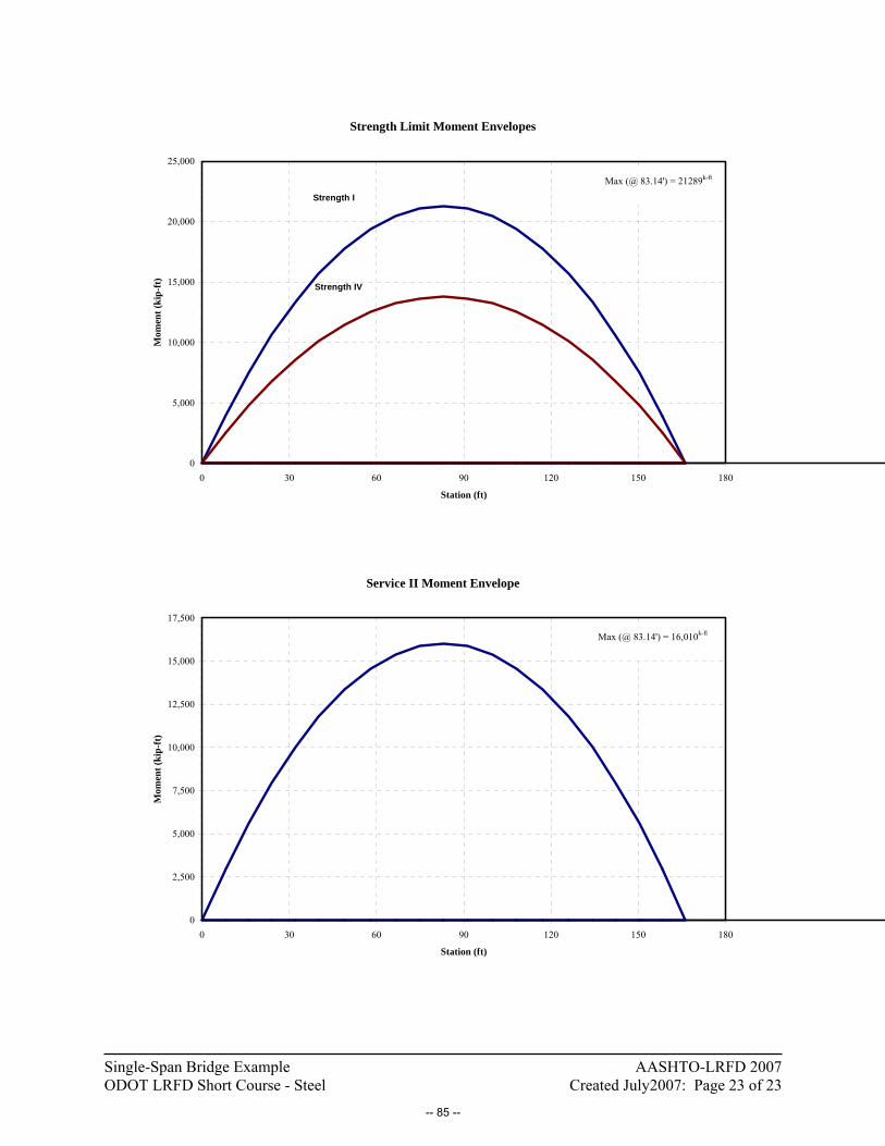
Single-Span Bridge Example AASHTO-LRFD 2007 ODOT LRFD Short Course - Steel Created July2007: Page 23 of 23
Strength Limit Moment Envelopes
0
5,000
10,000
15,000
20,000
25,000
0 30 60 90 120 150 180
Station (ft)
Mom
ent (
kip-
ft)
Strength I
Strength IV
Max (@ 83.14') = 21289k-ft
Service II Moment Envelope
0
2,500
5,000
7,500
10,000
12,500
15,000
17,500
0 30 60 90 120 150 180
Station (ft)
Mom
ent (
kip-
ft)
Max (@ 83.14') = 16,010k-ft
-- 85 --

-- 86 --

Single-Span Truss Bridge Example AASHTO-LRFD 2007 ODOT LRFD Short Course - Steel Created July 2007: Page 1 of 17
SINGLE-SPAN TRUSS BRIDGE DESIGN EXAMPLE 1. PROBLEM STATEMENT AND ASSUMPTIONS: Consider the truss bridge shown in Figure 1 below. The truss is simply supported with a span length of 112’–0” and a width (c-c of the trusses) of 19’–6”. The truss is made up of 7 panels that are each 16’-0” in length. Floor beams span between the truss panel points perpendicular to traffic and support stringers that span 16’-0” in the direction of traffic. Finally, the noncomposite W10 x 88 stringers support a 6” thick reinforced concrete deck. The simply supported stringers (6 across in each panel) are spaced at 3’ - 6” laterally. 1) Determine maximum and minimum axial forces in members 1-2, 1-4, 9-11, 9-10, and 10-13
due to an HL-93 Loading. 2) Determine the maximum moment in the stringer members due to the HL-93 Loading The entire truss superstructure is made up of W14 x 109 members except for the bottom chord, which is made up of MC 12 x 35 members. You may assume that the trucks drive down the center of the bridge (they really do, by the way) and as a result, the truck loads are approximately equally distributed between the trusses. To be on the safe side, however, assume that each truss carries 75% of the single lane. Model the truss as a determinate structure with pinned joints even though the actual truss has very few joints that are truly pinned. You may use a computer program for your truss analysis if you wish. I would suggest that you use SAP2000, Visual Analysis, or another similar FE package to model the truss. Disregard the lower limit of L = 20’ on the span length for computing distribution factors for the stringer members. Think about what is appropriate for the multiple presence factor.
Figure 1 - Tyler Road Bridge, Delaware County, OH
-- 87 --
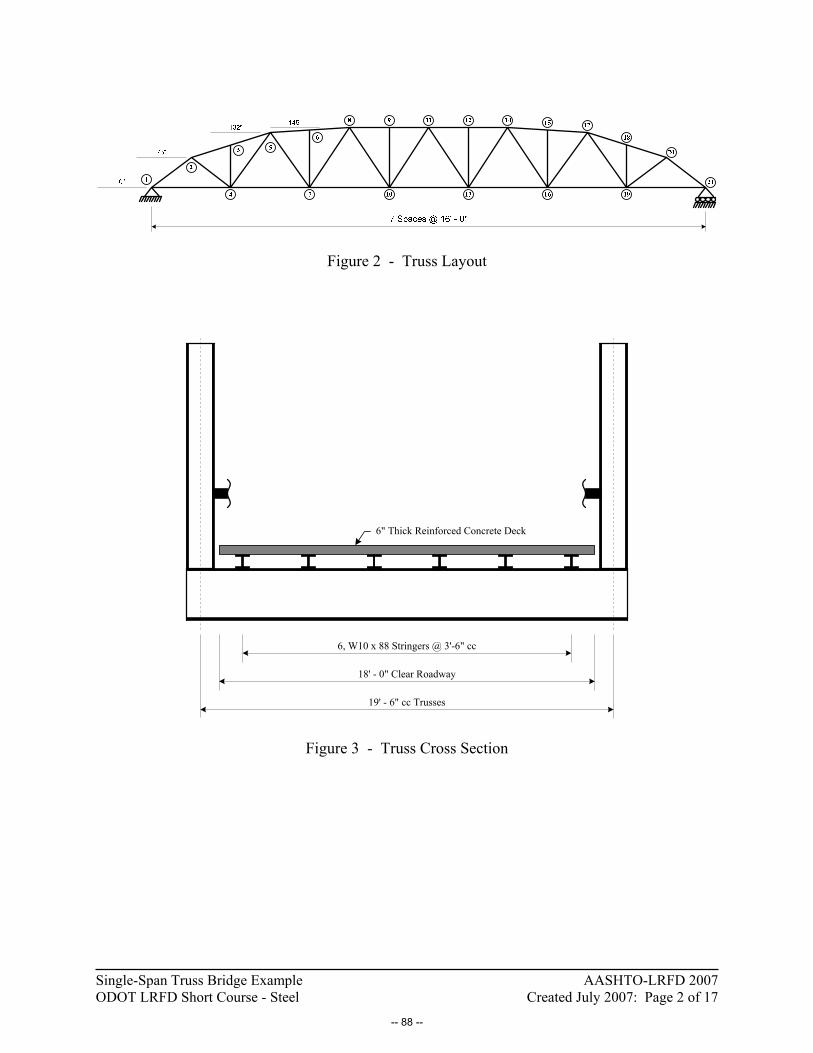
Single-Span Truss Bridge Example AASHTO-LRFD 2007 ODOT LRFD Short Course - Steel Created July 2007: Page 2 of 17
Figure 2 - Truss Layout
18' - 0" Clear Roadway
19' - 6" cc Trusses
6, W10 x 88 Stringers @ 3'-6" cc
6" Thick Reinforced Concrete Deck
Figure 3 - Truss Cross Section
-- 88 --

Single-Span Truss Bridge Example AASHTO-LRFD 2007 ODOT LRFD Short Course - Steel Created July 2007: Page 3 of 17
Compute the Maximum and Minimum Forces in Critical Members of the Truss: The following Influence Lines were obtained from SAP 2000:
-- 89 --
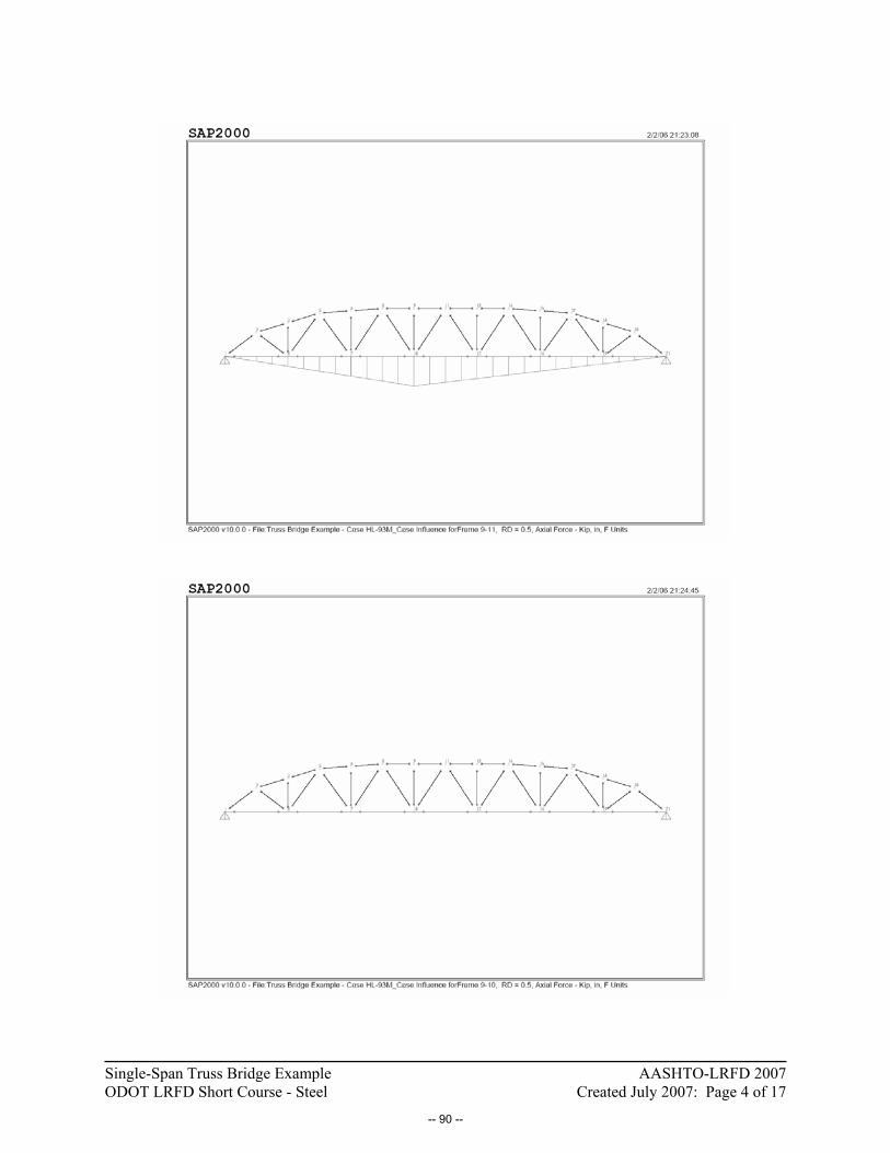
Single-Span Truss Bridge Example AASHTO-LRFD 2007 ODOT LRFD Short Course - Steel Created July 2007: Page 4 of 17
-- 90 --

Single-Span Truss Bridge Example AASHTO-LRFD 2007 ODOT LRFD Short Course - Steel Created July 2007: Page 5 of 17
-- 91 --
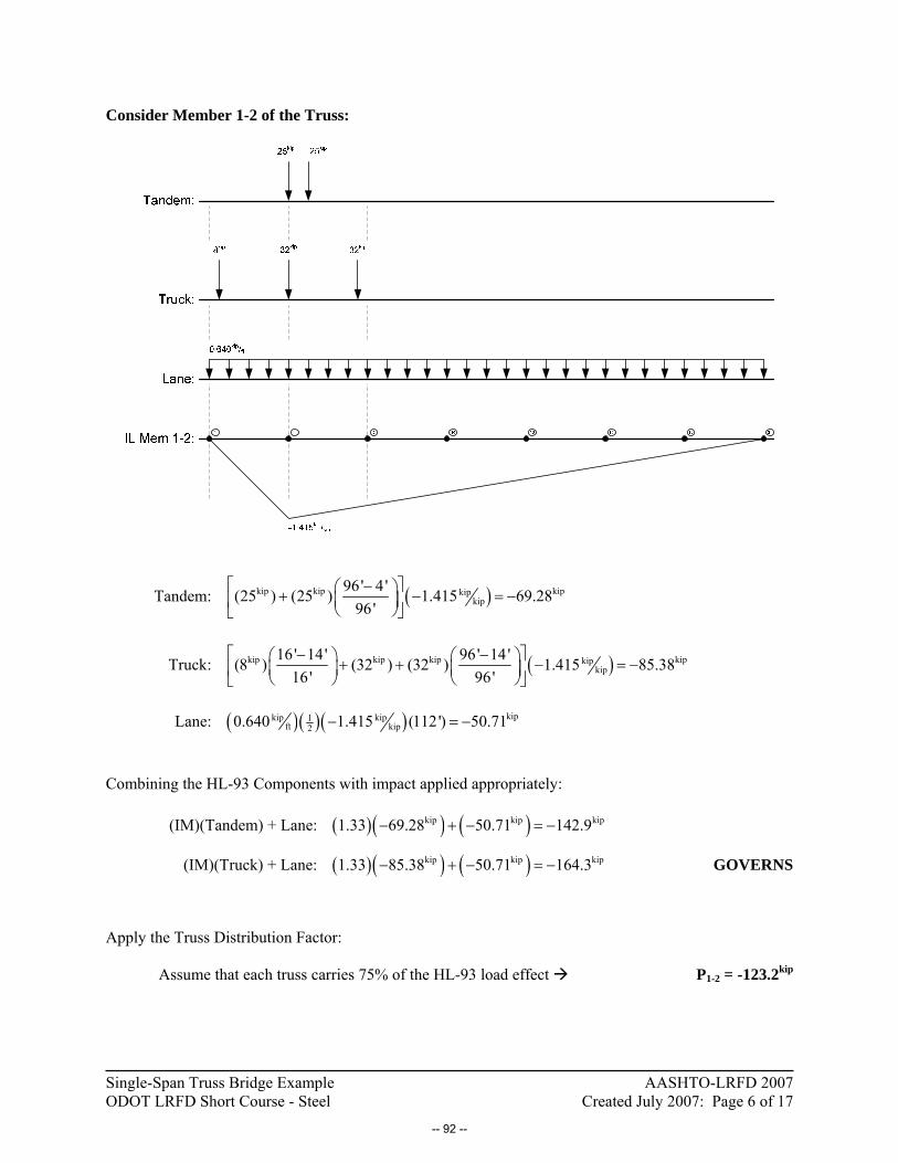
Single-Span Truss Bridge Example AASHTO-LRFD 2007 ODOT LRFD Short Course - Steel Created July 2007: Page 6 of 17
Consider Member 1-2 of the Truss:
Tandem: ( )kip kip kipkipkip
96' 4 '(25 ) (25 ) 1.415 69.2896'
⎡ ⎤−⎛ ⎞+ − = −⎜ ⎟⎢ ⎥⎝ ⎠⎣ ⎦
Truck: ( )kip kip kip kipkipkip
16' 14' 96' 14'(8 ) (32 ) (32 ) 1.415 85.3816' 96'
⎡ ⎤− −⎛ ⎞ ⎛ ⎞+ + − = −⎜ ⎟ ⎜ ⎟⎢ ⎥⎝ ⎠ ⎝ ⎠⎣ ⎦
Lane: ( )( )( ) kipkip kip1
ft kip20.640 1.415 (112') 50.71− = − Combining the HL-93 Components with impact applied appropriately: (IM)(Tandem) + Lane: ( )( ) ( )kip kip kip1.33 69.28 50.71 142.9− + − = −
(IM)(Truck) + Lane: ( )( ) ( )kip kip kip1.33 85.38 50.71 164.3− + − = − GOVERNS
Apply the Truss Distribution Factor: Assume that each truss carries 75% of the HL-93 load effect P1-2 = -123.2kip
-- 92 --
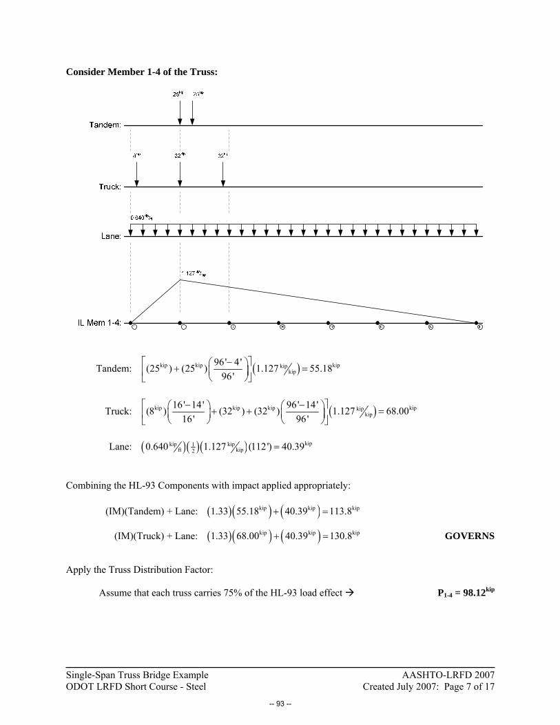
Single-Span Truss Bridge Example AASHTO-LRFD 2007 ODOT LRFD Short Course - Steel Created July 2007: Page 7 of 17
Consider Member 1-4 of the Truss:
Tandem: ( )kip kip kipkipkip
96' 4 '(25 ) (25 ) 1.127 55.1896'
⎡ ⎤−⎛ ⎞+ =⎜ ⎟⎢ ⎥⎝ ⎠⎣ ⎦
Truck: ( )kip kip kip kipkipkip
16 ' 14' 96' 14'(8 ) (32 ) (32 ) 1.127 68.0016' 96'
⎡ ⎤− −⎛ ⎞ ⎛ ⎞+ + =⎜ ⎟ ⎜ ⎟⎢ ⎥⎝ ⎠ ⎝ ⎠⎣ ⎦
Lane: ( )( )( ) kipkip kip1
ft kip20.640 1.127 (112') 40.39= Combining the HL-93 Components with impact applied appropriately: (IM)(Tandem) + Lane: ( )( ) ( )kip kip kip1.33 55.18 40.39 113.8+ =
(IM)(Truck) + Lane: ( )( ) ( )kip kip kip1.33 68.00 40.39 130.8+ = GOVERNS
Apply the Truss Distribution Factor: Assume that each truss carries 75% of the HL-93 load effect P1-4 = 98.12kip
-- 93 --

Single-Span Truss Bridge Example AASHTO-LRFD 2007 ODOT LRFD Short Course - Steel Created July 2007: Page 8 of 17
Consider Member 9-11 of the Truss:
Tandem: ( )kip kip kipkipkip
64' 4 '(25 ) (25 ) 2.254 109.264'
⎡ ⎤−⎛ ⎞+ − = −⎜ ⎟⎢ ⎥⎝ ⎠⎣ ⎦
Truck: ( )kip kip kip kipkipkip
48' 14' 64' 14'(8 ) (32 ) (32 ) 2.254 141.348' 64'
⎡ ⎤− −⎛ ⎞ ⎛ ⎞+ + − = −⎜ ⎟ ⎜ ⎟⎢ ⎥⎝ ⎠ ⎝ ⎠⎣ ⎦
Lane: ( )( )( ) kipkip kip1
ft kip20.640 2.254 (112') 80.78− = − Combining the HL-93 Components with impact applied appropriately: (IM)(Tandem) + Lane: ( )( ) ( )kip kip kip1.33 109.2 80.78 226.0− + − = −
(IM)(Truck) + Lane: ( )( ) ( )kip kip kip1.33 141.3 80.78 268.6− + − = − GOVERNS
Apply the Truss Distribution Factor: Assume that each truss carries 75% of the HL-93 load effect P9-11 = -201.5kip
-- 94 --

Single-Span Truss Bridge Example AASHTO-LRFD 2007 ODOT LRFD Short Course - Steel Created July 2007: Page 9 of 17
Consider Member 9-10 of the Truss: Member 9-10 of the truss is a zero force member. It may see some bending moment due to its rigid connection to the floor beam but it will not experience a net axial force due to live load. P9-10 = 0.000kip
-- 95 --
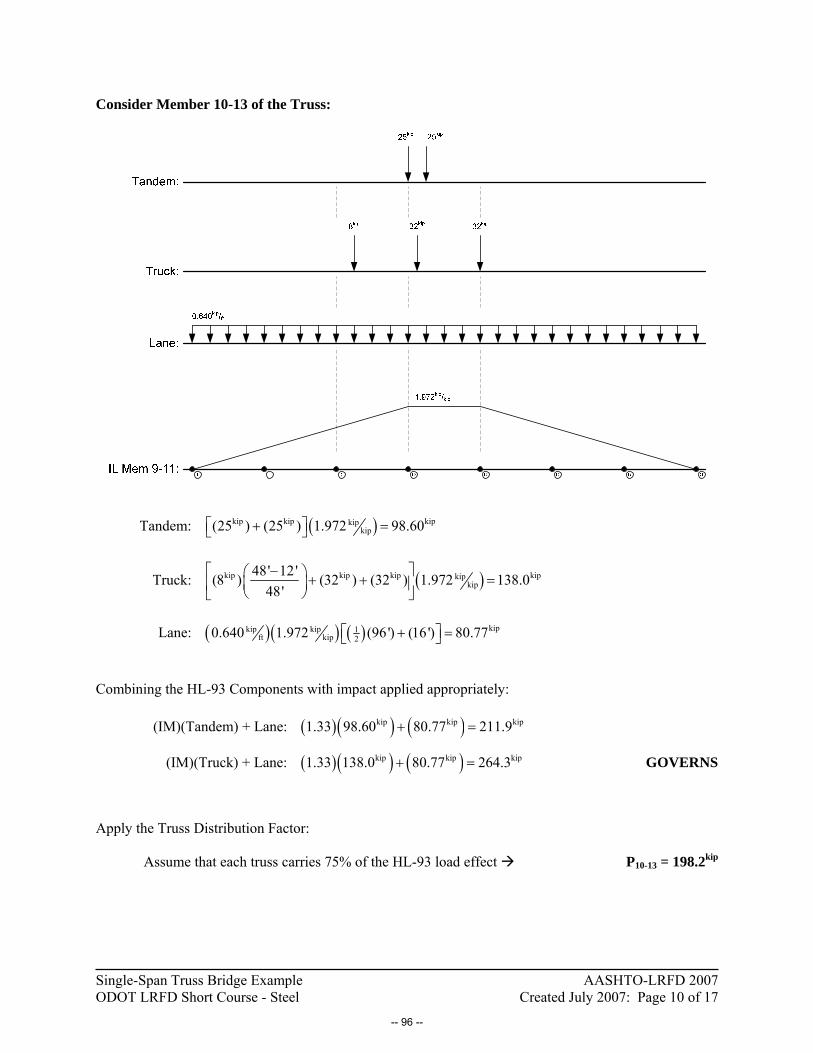
Single-Span Truss Bridge Example AASHTO-LRFD 2007 ODOT LRFD Short Course - Steel Created July 2007: Page 10 of 17
Consider Member 10-13 of the Truss:
Tandem: ( )kip kip kipkip
kip(25 ) (25 ) 1.972 98.60⎡ ⎤+ =⎣ ⎦
Truck: ( )kip kip kip kipkipkip
48' 12'(8 ) (32 ) (32 ) 1.972 138.048'
⎡ ⎤−⎛ ⎞ + + =⎜ ⎟⎢ ⎥⎝ ⎠⎣ ⎦
Lane: ( )( ) ( ) kipkip kip 1
ft kip 20.640 1.972 (96') (16') 80.77⎡ ⎤+ =⎣ ⎦ Combining the HL-93 Components with impact applied appropriately: (IM)(Tandem) + Lane: ( )( ) ( )kip kip kip1.33 98.60 80.77 211.9+ =
(IM)(Truck) + Lane: ( )( ) ( )kip kip kip1.33 138.0 80.77 264.3+ = GOVERNS
Apply the Truss Distribution Factor: Assume that each truss carries 75% of the HL-93 load effect P10-13 = 198.2kip
-- 96 --
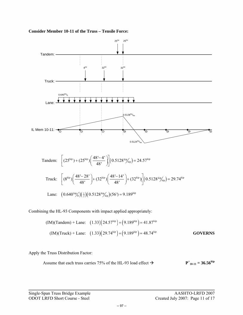
Single-Span Truss Bridge Example AASHTO-LRFD 2007 ODOT LRFD Short Course - Steel Created July 2007: Page 11 of 17
Consider Member 10-11 of the Truss – Tensile Force:
8kip 32kip 32kip
25kip 25kip
0.640kip/ft
0.5128kip/kip
Tandem:
Truck:
Lane:
IL Mem 10-11:
0.5124kip/kip
1 4 7 10 13 16 19 21
Tandem: ( )kip kip kipkipkip
48' 4 '(25 ) (25 ) 0.5128 24.5748'
⎡ ⎤−⎛ ⎞+ =⎜ ⎟⎢ ⎥⎝ ⎠⎣ ⎦
Truck: ( )kip kip kip kipkipkip
48' 28' 48' 14'(8 ) (32 ) (32 ) 0.5128 29.7448' 48'
⎡ ⎤− −⎛ ⎞ ⎛ ⎞+ + =⎜ ⎟ ⎜ ⎟⎢ ⎥⎝ ⎠ ⎝ ⎠⎣ ⎦
Lane: ( )( )( ) kipkip kip1
ft kip20.640 0.5128 (56') 9.189= Combining the HL-93 Components with impact applied appropriately: (IM)(Tandem) + Lane: ( )( ) ( )kip kip kip1.33 24.57 9.189 41.87+ =
(IM)(Truck) + Lane: ( )( ) ( )kip kip kip1.33 29.74 9.189 48.74+ = GOVERNS
Apply the Truss Distribution Factor: Assume that each truss carries 75% of the HL-93 load effect P+
10-11 = 36.56kip
-- 97 --

Single-Span Truss Bridge Example AASHTO-LRFD 2007 ODOT LRFD Short Course - Steel Created July 2007: Page 12 of 17
Consider Member 10-11 of the Truss – Compressive Force:
8kip32kip32kip
25kip 25kip
0.640kip/ft
0.5128kip/kip
Tandem:
Truck:
Lane:
IL Mem 10-11:
0.5124kip/kip
1 4 7 10 13 16 19 21
Tandem: ( )kip kip kipkipkip
48' 4 '(25 ) (25 ) 0.5124 24.5548'
⎡ ⎤−⎛ ⎞+ − = −⎜ ⎟⎢ ⎥⎝ ⎠⎣ ⎦
Truck: ( )kip kip kip kipkipkip
48' 28' 48' 14'(8 ) (32 ) (32 ) 0.5124 29.7248' 48'
⎡ ⎤− −⎛ ⎞ ⎛ ⎞+ + − = −⎜ ⎟ ⎜ ⎟⎢ ⎥⎝ ⎠ ⎝ ⎠⎣ ⎦
Lane: ( )( )( ) kipkip kip1
ft kip20.640 0.5124 (56') 9.182− = − Combining the HL-93 Components with impact applied appropriately: (IM)(Tandem) + Lane: ( )( ) ( )kip kip kip1.33 24.55 9.182 41.83− + − = −
(IM)(Truck) + Lane: ( )( ) ( )kip kip kip1.33 29.72 9.182 48.71− + − = − GOVERNS
Apply the Truss Distribution Factor: Assume that each truss carries 75% of the HL-93 load effect P-
10-11 = -36.53kip
-- 98 --
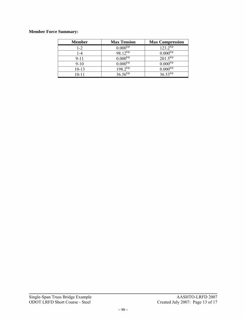
Single-Span Truss Bridge Example AASHTO-LRFD 2007 ODOT LRFD Short Course - Steel Created July 2007: Page 13 of 17
Member Force Summary:
Member Max Tension Max Compression 1-2 0.000kip 123.2kip 1-4 98.12kip 0.000kip
9-11 0.000kip 201.5kip 9-10 0.000kip 0.000kip
10-13 198.2kip 0.000kip 10-11 36.56kip 36.53kip
-- 99 --

Single-Span Truss Bridge Example AASHTO-LRFD 2007 ODOT LRFD Short Course - Steel Created July 2007: Page 14 of 17
Compute the Moment Distribution Factor for the Stringers in the Floor System: Interior Girder –
One Lane Loaded:
0.10.4 0.3
1, 3
2
4 2 2
4
0.10.4 0.3 4
1, 3
1,
0.0614 12
( )
(8)(534 in (25.9 in )(8.40") )
18,890 in
3.5 ' 3.5 ' 18,890 in0.06
14 16 ' 12(16 ')(6.0")
gM Int
s
g g
g
g
M Int
M Int
KS SDF
L Lt
K n I Ae
K
K
DF
DF
= +
= +
= +
=
= +
=
⎛ ⎞⎛ ⎞ ⎛ ⎞⎜ ⎟ ⎜ ⎟ ⎜ ⎟⎝ ⎠ ⎝ ⎠ ⎝ ⎠
⎛ ⎞⎛ ⎞ ⎛ ⎞⎜ ⎟ ⎜ ⎟ ⎜ ⎟⎝ ⎠ ⎝ ⎠ ⎝ ⎠
0.3965
Two or More Lanes Loaded:
The bridge is designed for a single traffic lane. Exterior Girder –
One Lane Loaded:
The lever rule is applied by assuming that a hinge forms over the first interior stringer as a truck load is applied near the guard rail. The resulting reaction in the exterior stringer is the distribution factor.
( )
1,
1.75')0.2500
(3.50 ') 0.2500
/ 2 (
M Ext
P
DF
PR = =
=
The Multiple Presence Factor would generally be applied but in this case, there is only a single design lane so it is not used.
Two or More Lanes Loaded:
The bridge is designed for a single traffic lane.
Minimum Exterior Girder Distribution Factor:
-- 100 --

Single-Span Truss Bridge Example AASHTO-LRFD 2007 ODOT LRFD Short Course - Steel Created July 2007: Page 15 of 17
,
2
L
Ext Minb
N
ExtL
Nb
X eN
DFN
x= +
∑
∑
One Lane Loaded:
8'-9"
P/2 P/2
3'-0"2'-0"
1'-9"
5'-3"
3'-0"
4'-0"
1, , 2 2 2
1 (4.00 ')(8.75')0.3299
6 (2) (8.75') (5.25') (1.75')M Ext MinDF = + =
+⎡ ⎤+⎣ ⎦
The Multiple Presence Factor would generally be applied but in this case, there is only a single design lane so it is not used.
Moment Distribution Factor Summary: Interior Stringer: DFM1,Int = 0.3965 Exterior Stringer (Lever Rule): DFM1, Ext = 0.2500 Exterior Stringer (Minimum): DFM1, Ext = 0.3299
For simplicity, take the moment distribution factor as 0.3965 for all stringers.
-- 101 --
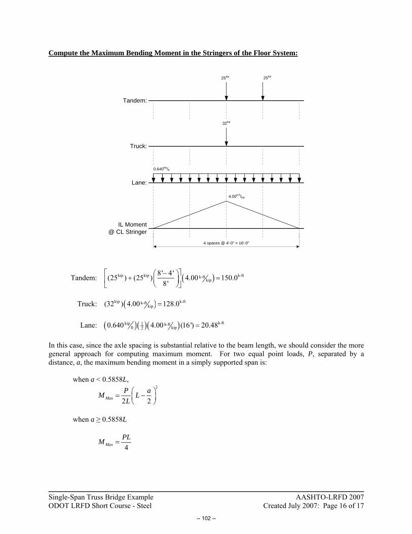
Single-Span Truss Bridge Example AASHTO-LRFD 2007 ODOT LRFD Short Course - Steel Created July 2007: Page 16 of 17
Compute the Maximum Bending Moment in the Stringers of the Floor System:
32kip
25kip 25kip
0.640kip/ft
Tandem:
Truck:
Lane:
IL Moment@ CL Stringer
4.00k-ft/kip
4 spaces @ 4'-0" = 16'-0"
Tandem: ( )kip kip k-ftk-ftkip
8' 4 '(25 ) (25 ) 4.00 150.08'
⎡ ⎤−⎛ ⎞+ =⎜ ⎟⎢ ⎥⎝ ⎠⎣ ⎦
Truck: ( )kip k-ftk-ft
kip(32 ) 4.00 128.0= Lane: ( )( )( ) k-ftkip 1 k-ft
ft kip20.640 4.00 (16') 20.48= In this case, since the axle spacing is substantial relative to the beam length, we should consider the more general approach for computing maximum moment. For two equal point loads, P, separated by a distance, a, the maximum bending moment in a simply supported span is: when a < 0.5858L,
2
2 2MaxP aM LL⎛ ⎞= −⎜ ⎟⎝ ⎠
when a ≥ 0.5858L
4Max
PLM =
-- 102 --

Single-Span Truss Bridge Example AASHTO-LRFD 2007 ODOT LRFD Short Course - Steel Created July 2007: Page 17 of 17
Tandem: 2kip
k-ft(25 ) 4'16' 153.1(2)(16') 2MaxM ⎛ ⎞= − =⎜ ⎟
⎝ ⎠ (an increase of 2.067%)
Truck: kip
k-ft(32 )(16') 128.0(4)MaxM = = (no change)
Combining the HL-93 Components with impact applied appropriately: (IM)(Tandem) + Lane: ( )( ) ( )k-ft k-ft k-ft1.33 153.1 20.48 224.1+ = GOVERNS
(IM)(Truck) + Lane: ( )( ) ( )k-ft k-ft k-ft1.33 128.0 20.48 190.7+ =
Apply the Stringer Distribution Factor: Each stringer carries 0.3965 lanes of the HL-93 loading MStringer = 88.86k-ft
-- 103 --

-- 104 --
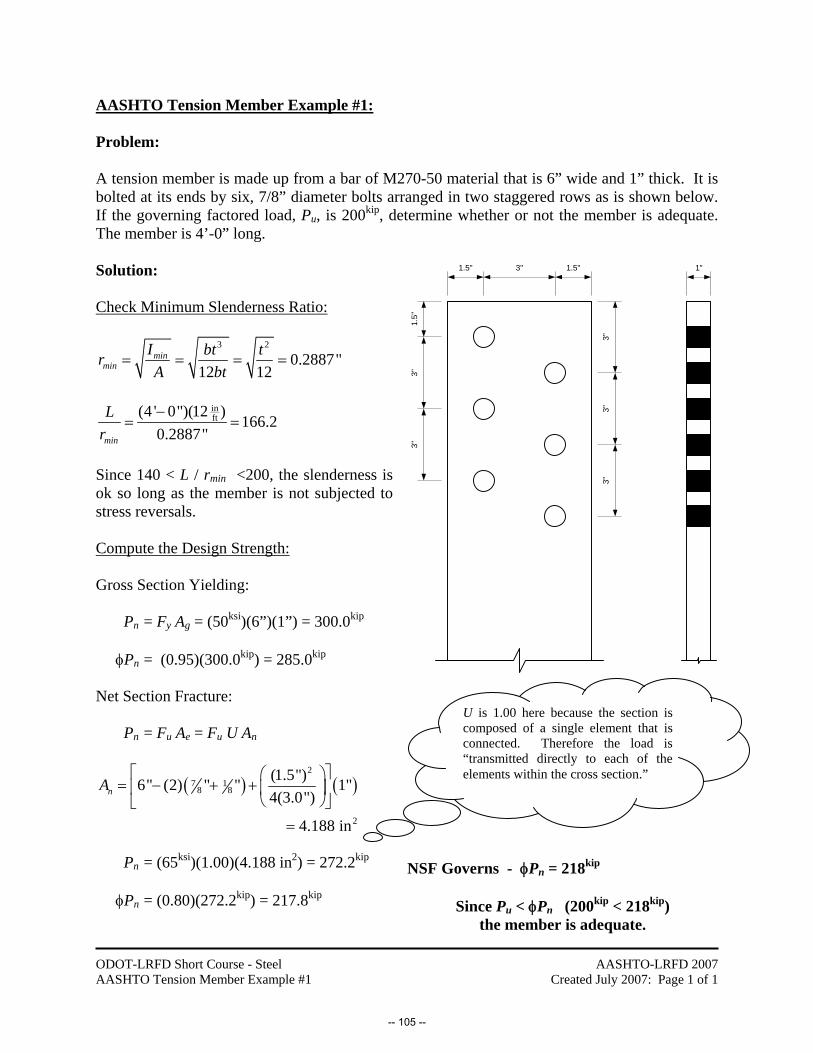
ODOT-LRFD Short Course - Steel AASHTO Tension Member Example #1
AASHTO-LRFD 2007 Created July 2007: Page 1 of 1
AASHTO Tension Member Example #1: Problem: A tension member is made up from a bar of M270-50 material that is 6” wide and 1” thick. It is bolted at its ends by six, 7/8” diameter bolts arranged in two staggered rows as is shown below. If the governing factored load, Pu, is 200kip, determine whether or not the member is adequate. The member is 4’-0” long. Solution: Check Minimum Slenderness Ratio:
3 2
0.2887"12 12
minmin
I bt trA bt
= = = =
inft(4 ' 0")(12 ) 166.2
0.2887"min
Lr
−= =
Since 140 < L / rmin <200, the slenderness is ok so long as the member is not subjected to stress reversals. Compute the Design Strength: Gross Section Yielding: Pn = Fy Ag = (50ksi)(6”)(1”) = 300.0kip φPn = (0.95)(300.0kip) = 285.0kip Net Section Fracture: Pn = Fu Ae = Fu U An
( ) ( )2
7 18 8
2
(1.5")6" (2) " " 1"4(3.0")
4.188 in
nA⎡ ⎤⎛ ⎞
= − + +⎢ ⎥⎜ ⎟⎝ ⎠⎣ ⎦
=
Pn = (65ksi)(1.00)(4.188 in2) = 272.2kip
φPn = (0.80)(272.2kip) = 217.8kip
3" 1"
1.5"
3"3"
3"3"
3"
1.5" 1.5"
NSF Governs - φPn = 218kip
Since Pu < φPn (200kip < 218kip) the member is adequate.
U is 1.00 here because the section is composed of a single element that is connected. Therefore the load is “transmitted directly to each of the elements within the cross section.”
-- 105 --
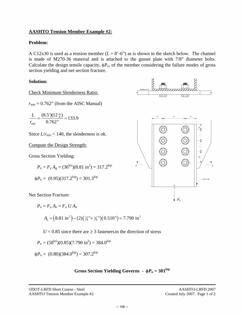
ODOT-LRFD Short Course - Steel AASHTO Tension Member Example #2
AASHTO-LRFD 2007 Created July 2007: Page 1 of 2
AASHTO Tension Member Example #2: Problem: A C12x30 is used as a tension member (L = 8’-6”) as is shown in the sketch below. The channel is made of M270-36 material and is attached to the gusset plate with 7/8” diameter bolts. Calculate the design tensile capacity, φPn, of the member considering the failure modes of gross section yielding and net section fracture. Solution: Check Minimum Slenderness Ratio: rmin = 0.762” (from the AISC Manual)
inft(8.5 ')(12 ) 133.9
0.762"min
Lr
= =
Since L/rmin < 140, the slenderness is ok. Compute the Design Strength: Gross Section Yielding: Pn = Fy Ag = (36ksi)(8.81 in2) = 317.2kip φPn = (0.95)(317.2kip) = 301.3kip Net Section Fracture: Pn = Fu Ae = Fu U An
A
3"3" 6"
Pu
A
Section A-A
C12 x 30
( ) ( )( )2 27 1
8 88.81 in (2) " " 0.510" 7.790 innA = − + = U = 0.85 since there are ≥ 3 fasteners in the direction of stress Pn = (58ksi)(0.85)(7.790 in2) = 384.0kip
φPn = (0.80)(384.0kip) = 307.2kip
Gross Section Yielding Governs - φPn = 301kip
-- 106 --

ODOT-LRFD Short Course - Steel AASHTO Tension Member Example #2
AASHTO-LRFD 2007 Created July 2007: Page 2 of 2
Side Note:
Note that if the AISC shear lag provisions were used that Case 2 from AISC Table D3.1 would apply:
0.674"1 1 0.92519.00"
xUL
= − = − = …. for net section fracture, φPn = 334.3kip
In this case, however, the design strength is unaffected since gross yielding governs.
-- 107 --

ODOT-LRFD Short Course - Steel AASHTO Tension Member Example #3
AASHTO-LRFD 2007 Created July 2007: Page 1 of 2
AASHTO Tension Member Example #3: Problem: Determine the design strength of the W10x60 member of M270-50 steel. As is shown, the member is connected to two gusset plates – one on each flange. The end connection has two lines of 3/4” diameter bolts in each flange - five in each line.
A
ASection A-A
5 spaces @ 3”
W10 x 60
Gusset Plates
Solution: Check Minimum Slenderness Ratio:
rmin = 2.57” (from the AISC Manual)
min
1402.57"
L Lr
= ≤ this is satisfied so long as L ≤ 359.8” = 29’-113/4”
Compute the Design Strength: Gross Section Yielding: Pn = Fy Ag = (50ksi)(17.6 in2) = 880.0kip φPn = (0.95)(880.0kip) = 836.0kip
-- 108 --

ODOT-LRFD Short Course - Steel AASHTO Tension Member Example #3
AASHTO-LRFD 2007 Created July 2007: Page 2 of 2
Net Section Fracture: Pn = Fu Ae = Fu U An ( ) ( )( )2 23 1
4 817.6 in (4) " " 0.680" 15.22 innA = − + =
Check ?
23fb d≥ … ( ) ( )( )
?2
310.1" 10.2"≥ OK U = 0.90 since bf > 2/3d and there are ≥ 3 fasteners in the direction of stress.
Pn = (65ksi)(0.90)(15.22 in2) = 890.4kip
φPn = (0.80)(890.4kip) = 712.3kip
Net Section Fracture Governs - φPn =712kip
Side Note:
Note that if the AISC shear lag provisions were used that Case 7a from AISC Table D3.1 would apply:
Check ?
23fb d≥
( ) ( )( )?
2310.1" 10.2"≥ OK
∴ U = 0.90 Alternatively, Table D3.1 Case 2 can be applied:
0.884"1 1 0.926312.0"
xUL
= − = − =
The value of U = 0.9263 can be used. Pn = (65ksi)(0.9263)(15.22 in2) = 916.4kip
φPn = (0.80)(916.4kip) = 733.1kip
x x
The connection eccentricity x is taken as the distance from the faying surface to the CG of a WT5x30.
Since Net Section Fracture governs the capacity of this member, the overall design strength of the member would be increased to 733kip.
-- 109 --

ODOT-LRFD Short Course - Steel AASHTO Tension Member Example #4
AASHTO-LRFD 2007 Created July 2007: Page 1 of 1
AASHTO Tension Member Example #4: Problem: An L6x4x1/2, M270-36, is welded to a gusset plate. The long leg of the angle is attached using two, 8” long fillet welds. Compute the strength of the angle in tension. Solution: Check Minimum Slenderness Ratio:
rmin = rz = 0.864” (from the AISC Manual)
2400.864"min
L Lr
= ≤
this is satisfied so long as L ≤ 207.4” = 17’-33/8”
Compute the Design Strength: Gross Section Yielding: Pn = Fy Ag = (36ksi)(4.75 in2) = 171.0kip φPn = (0.95)(171.0kip) = 162.5kip Net Section Fracture: Pn = Fu Ae = Fu U An Lacking other guidance, AISC Table D3.1 Case 2 will be applied:
0.981"1 1 0.87748.0"
xUL
= − = − =
Pn = (58ksi) (0.8774)(4.75 in2) = 241.7kip φPn = (0.80)(241.7kip) = 193.4kip
Gross Section Yielding Governs - φPn =163kip
-- 110 --

ODOT-LRFD Short Course - Steel AASHTO Compression Member Example #1
AASHTO-LRFD 2007 Created July 2007: Page 1 of 1
AASHTO Compression Member Example #1: Problem: Compute the design compressive strength of a W14x74 made of M270-50 steel. The column has a length of 20 ft and can be treated as pinned-pinned. Solution: Check Local Buckling:
Flange: ?
2f
f y
b Ekt F≤ λf = 6.41 (Tabulated)
? 29,0006.41 0.56 13.550
≤ = OK
Web: ?
w y
h Ekt F≤ λw = 25.4 (Tabulated)
? 29,00025.4 1.49 35.950
≤ = OK
Compute Flexural Buckling Capacity: Slenderness Ratios:
inft
inft
(1.00)(20 ')(12 ) 39.74 120 OK6.04"
(1.00)(20 ')(12 ) 96.77 120 OK2.48"
x
y
KLr
KLr
⎛ ⎞ = = <⎜ ⎟⎝ ⎠
⎛ ⎞ = = <⎜ ⎟⎝ ⎠
Since the effective slenderness ratio is larger for the y axis than the x axis, y-axis buckling will govern. 2 2 ksi
ksi
96.77 50 1.63629,000
y
y
FKLr E
⎛ ⎞⎛ ⎞ ⎛ ⎞λ = = =⎜ ⎟⎜ ⎟ ⎜ ⎟π π⎝ ⎠ ⎝ ⎠ ⎝ ⎠
(6.9.4.1-3)
Since λ ≤ 2.25, Inelastic Buckling Governs
( )( )( )( )1.636 ksi 2 kip0.66 0.66 50 21.8 in 549.6n y sP F Aλ= = = (6.9.4.1-1)
φPn = (0.90)(549.6kip) φPn = 495kip
-- 111 --
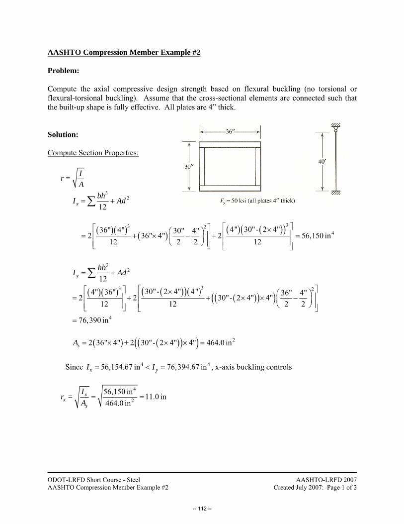
ODOT-LRFD Short Course - Steel AASHTO Compression Member Example #2
AASHTO-LRFD 2007 Created July 2007: Page 1 of 2
AASHTO Compression Member Example #2 Problem: Compute the axial compressive design strength based on flexural buckling (no torsional or flexural-torsional buckling). Assume that the cross-sectional elements are connected such that the built-up shape is fully effective. All plates are 4” thick. Solution: Compute Section Properties:
Ir =A
32
12xbhI Ad= +∑
( )( ) ( ) ( ) ( )( )33 2 4" 30"- 2 4"36" 4" 30" 4"2 36" 4" 212 2 2 12
⎡ ⎤⎡ ⎤ ×⎛ ⎞ ⎢ ⎥= + × − +⎢ ⎥⎜ ⎟ ⎢ ⎥⎝ ⎠⎢ ⎥⎣ ⎦ ⎣ ⎦
456,150 in=
3
2
12yhbI Ad= +∑
( )( ) ( )( )( ) ( )( )( )33 230"- 2 4" 4"4" 36" 36" 4"2 2 30"- 2 4" 4"
12 12 2 2
⎡ ⎤⎡ ⎤ × ⎛ ⎞⎢ ⎥= + + × × −⎢ ⎥ ⎜ ⎟⎢ ⎥⎝ ⎠⎢ ⎥⎣ ⎦ ⎣ ⎦
476,390 in=
( ) ( )( )( ) 22 36" 4" + 2 30"- 2 4" 4" 464.0 insA = × × × =
Since 4 456,154.67 in 76,394.67 inx yI I= < = , x-axis buckling controls
4
256,150 in 11.0 in464.0 in
xx
s
Ir =A
= =
-- 112 --

ODOT-LRFD Short Course - Steel AASHTO Compression Member Example #2
AASHTO-LRFD 2007 Created July 2007: Page 2 of 2
Check Local Buckling (Section 6.9.4.2):
( )36" 2 4"7.00
4"bt
−= =
?
y
b Ekt F≤ (6.9.4.2-1)
ksi
ksi29,0007.00 1.40 33.72
50≤ = OK
Calculate the Nominal Compressive Strength (Section E3 page 16.1-33):
Slenderness Ratios: KLr
where:
0.8K = (Section 4.6.2.5)
inft40 ft 12 480"x yL L= = × =
( )( )( )
0.8 480 in34.91
11.0 inx
x
KLr
= =
2 2 ksi
ksi34.91 50 0.2129
29,000y
s
FKLr E
⎛ ⎞ ⎛ ⎞λ = = =⎜ ⎟ ⎜ ⎟π π⎝ ⎠⎝ ⎠ (6.9.4.1-3)
Since 2.25λ ≤ , Inelastic Flexural Buckling Governs
( )( )0.2129 ksi 2 kip0.66 0.66 50 464.0 in 21,240n y sP F Aλ= = = (6.9.4.1-1)
( )( )kip kip
c 0.90 21,240 19,110nPφ = =
-- 113 --

ODOT-LRFD Short Course - Steel AASHTO Compression Member Example #3 v2
AASHTO-LRFD 2007 Created July 2007: Page 1 of 2
AASHTO Compression Member Example #3: Problem: Determine the effective length factor, K, for column AB in the frame shown below. Column AB is a W10x88 made of A992 steel. W16x36 beams frame into joint A and W16x77 beams frame into joint B. The frame is unbraced and all connections are rigid. Consider only buckling in the plane of the page about the sections’ strong axes.
W16 x 36
L=24'
W16 x 77
L=24'
W10 x 88
L=14'
A
B
4 @ 24'
8 @
14'
A
B
Solution:
-- 114 --
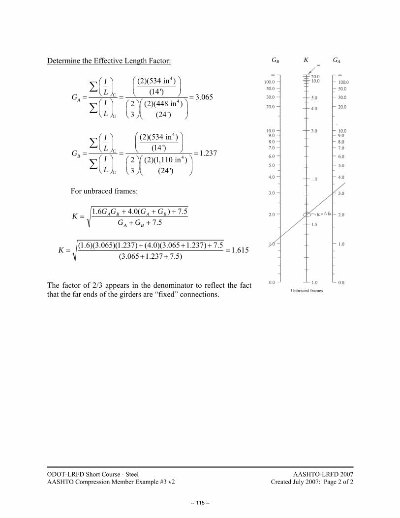
ODOT-LRFD Short Course - Steel AASHTO Compression Member Example #3 v2
AASHTO-LRFD 2007 Created July 2007: Page 2 of 2
Determine the Effective Length Factor:
4
4
(2)(534 in )(14 ')
3.0652 (2)(448 in )3 (24 ')
CA
G
ILGIL
⎛ ⎞⎛ ⎞⎜ ⎟⎜ ⎟
⎝ ⎠ ⎝ ⎠= = =⎛ ⎞ ⎛ ⎞⎛ ⎞⎜ ⎟ ⎜ ⎟⎜ ⎟⎝ ⎠ ⎝ ⎠⎝ ⎠
∑
∑
4
4
(2)(534 in )(14 ')
1.2372 (2)(1,110 in )3 (24 ')
CB
G
ILGIL
⎛ ⎞⎛ ⎞⎜ ⎟⎜ ⎟
⎝ ⎠ ⎝ ⎠= = =⎛ ⎞ ⎛ ⎞⎛ ⎞⎜ ⎟ ⎜ ⎟⎜ ⎟⎝ ⎠ ⎝ ⎠⎝ ⎠
∑
∑
For unbraced frames:
5.75.7)(0.46.1
+++++
=BA
BABA
GGGGGGK
(1.6)(3.065)(1.237) (4.0)(3.065 1.237) 7.5 1.615(3.065 1.237 7.5)
K + + += =
+ +
The factor of 2/3 appears in the denominator to reflect the fact that the far ends of the girders are “fixed” connections.
GB K GA
-- 115 --
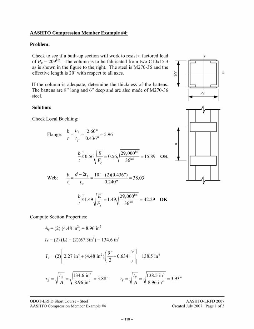
ODOT-LRFD Short Course - Steel AASHTO Compression Member Example #4
AASHTO-LRFD 2007 Created July 2007: Page 1 of 3
AASHTO Compression Member Example #4: Problem: Check to see if a built-up section will work to resist a factored load of Pu = 209kip. The column is to be fabricated from two C10x15.3as is shown in the figure to the right. The steel is M270-36 and the effective length is 20’ with respect to all axes.
If the column is adequate, determine the thickness of the battens.The battens are 8” long and 6” deep and are also made of M270-36 steel.
Solution: Check Local Buckling:
Flange: 2.60" 5.960.436"
f
f
bbt t= = =
ksi?
ksi
29,0000.56 0.56 15.8936y
b Et F≤ = = OK
Web: 2 10" (2)(0.436") 38.03
0.240"f
w
d tbt t
− −= = =
ksi?
ksi
29,0001.49 1.49 42.2936y
b Et F≤ = = OK
9"
a
x
y
10"
Compute Section Properties: As = (2) (4.48 in2) = 8.96 in2 IX = (2) (Ix) = (2)(67.3in4) = 134.6 in4
2
4 2 49"(2) 2.27 in (4.48 in ) 0.634" 138.5 in2YI
⎡ ⎤⎛ ⎞= + − =⎢ ⎥⎜ ⎟⎝ ⎠⎢ ⎥⎣ ⎦
4
2
134.6 in 3.88"8.96 in
XX
IrA
= = = 4
2
138.5 in 3.93"8.96 in
YY
IrA
= = =
-- 116 --

ODOT-LRFD Short Course - Steel AASHTO Compression Member Example #4
AASHTO-LRFD 2007 Created July 2007: Page 2 of 3
Slenderness Ratios:
inft(20 ')(12 ) 61.86
3.88"X
KLr
⎛ ⎞⎛ ⎞ = =⎜ ⎟ ⎜ ⎟⎝ ⎠ ⎝ ⎠
inft(20 ')(12 ) 61.07
3.93"Y
KLr
⎛ ⎞⎛ ⎞ = =⎜ ⎟ ⎜ ⎟⎝ ⎠ ⎝ ⎠
It appears as though X axis buckling will govern but since the battens will be subjected to shear if the section buckles about its Y axis, this slenderness ratio must be modified.
Batten Spacing:
34i
max
KLa rr
⎛ ⎞⎛ ⎞≤ ⎜ ⎟⎜ ⎟⎝ ⎠⎝ ⎠
ri = ry = 0.711” (for one channel) max X
KL KLr r
⎛ ⎞ ⎛ ⎞=⎜ ⎟ ⎜ ⎟⎝ ⎠ ⎝ ⎠
( )( )(0.711") 0.75 61.86a ≤
32.98"a ≤ use 9 battens @ a = 30”
Modified Slenderness Ratio – Y-axis Buckling:
The modified slenderness ratio is calculated as,
22 2
20.82(1 )m o ib
KL KL ar r r
αα
⎛ ⎞⎛ ⎞ ⎛ ⎞= + ⎜ ⎟⎜ ⎟ ⎜ ⎟ +⎝ ⎠ ⎝ ⎠ ⎝ ⎠ (6.9.4.3.1-1)
rib = 0.711” h = 9” – (2)(0.634”) = 7.73”
7.732" 5.442 (2)(0.711")ib
hr
α = = =
( ) ( )22
2
2
(5.44) 30"61.07 0.82 71.700.711"1 (5.44)m
KLr
⎛ ⎞⎛ ⎞ ⎛ ⎞⎜ ⎟= + =⎜ ⎟ ⎜ ⎟⎜ ⎟+⎝ ⎠ ⎝ ⎠⎝ ⎠
Now we can see that after the Y axis slenderness ratio is modified, Y axis buckling actually governs over X axis buckling.
-- 117 --

ODOT-LRFD Short Course - Steel AASHTO Compression Member Example #4
AASHTO-LRFD 2007 Created July 2007: Page 3 of 3
Column Design Capacity:
2 2 ksi
ksi
71.70 36 0.646629,000
y
y
FKLr E
⎛ ⎞⎛ ⎞ ⎛ ⎞λ = = =⎜ ⎟⎜ ⎟ ⎜ ⎟π π⎝ ⎠ ⎝ ⎠ ⎝ ⎠
(6.9.4.1-3)
Since λ ≤ 2.25, Inelastic Buckling Governs ( )( )( )( )0.6466 ksi 2 kip0.66 0.658 36 8.96 in 246.1n y sP F Aλ= = = (6.9.4.1-1)
φPn = (0.90)(246.1kip) φPn = 221kip Since φPn > ΣγQ, the column is adequate.
Batten Design: Assume that there are inflection points half way between the battens and design for a shear equal to 2% of the compressive design strength (AISC Section E6. Pg 16.1-39)
2Mu,Batten
2.21 kip
2.21 kip
Vu = (0.02)(221kip) = 4.42kip
kipkip
channel4.42 2.21
2=
ΣM Mu,Batten = 33.15k-in
3(6") 1812Batten
tI t= =
18 63Batten
tS t= =
for first yield, My = Fy S Let φFy S ≥ Mu,Batten
k-in
ksi 3
33.15(1.00)(36 )(6 in )
t ≥
t ≥ 0.153” use t = 5/16” (Min Thickness) use PL6 x 8 x 5/16 Battens
-- 118 --
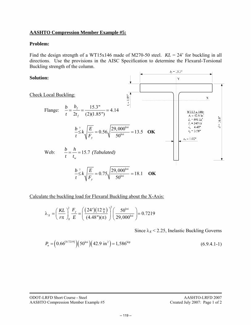
ODOT-LRFD Short Course - Steel AASHTO Compression Member Example #5
AASHTO-LRFD 2007 Created July 2007: Page 1 of 2
AASHTO Compression Member Example #5: Problem: Find the design strength of a WT15x146 made of M270-50 steel. KL = 24’ for buckling in all directions. Use the provisions in the AISC Specification to determine the Flexural-Torsional Buckling strength of the column. Solution:
Check Local Buckling:
Flange: 15.3" 4.142 (2)(1.85")
f
f
bbt t= = =
ksi?
ksi
29,0000.56 13.550y
b Ekt F≤ = = OK
Web: 15.7w
b ht t= = (Tabulated)
ksi?
ksi
29,0000.75 18.150y
b Ekt F≤ = = OK
Calculate the buckling load for Flexural Buckling about the X-Axis:
( )( ) 22 ksiinft
ksi
24 ' 12 50 0.7219(4.48")( ) 29,000
yX
X
FKLr E
⎛ ⎞ ⎛ ⎞⎛ ⎞λ = = =⎜ ⎟ ⎜ ⎟⎜ ⎟π π⎝ ⎠ ⎝ ⎠⎝ ⎠
Since λX < 2.25, Inelastic Buckling Governs
( )( )( )( )0.7219 ksi 2 kip0.66 50 42.9 in 1,586nP = = (6.9.4.1-1)
-- 119 --

ODOT-LRFD Short Course - Steel AASHTO Compression Member Example #5
AASHTO-LRFD 2007 Created July 2007: Page 2 of 2
Calculate the Critical Stress for Flexural-Torsional Buckling about the Y-axis:
( ), , , ,
2, ,
41 1
2cr Y cr Z cr Y cr Z
crft
cr Y cr Z
F F F F HF
H F F
⎛ ⎞+ ⎜ ⎟= − −⎜ ⎟+⎝ ⎠
(AISC E4-2)
( )( ) 22 ksiinft
ksi
24 ' 12 50 1.131(3.58")( ) 29,000
yY
Y
FKLr E
⎛ ⎞ ⎛ ⎞⎛ ⎞λ = = =⎜ ⎟ ⎜ ⎟⎜ ⎟π π⎝ ⎠ ⎝ ⎠⎝ ⎠
Since λY < 2.25, Inelastic Buckling Governs
( )( )( )1.131 ksi ksi
, 0.66 50 31.15ncr Y
s
PFA
= = = (6.9.4.1-1)
2 2 2 x y
o o og
I Ir x y
A+
= + + …… 1.85"3.62" 2.695"2oy = − = (AISC E4-7)
( )4 4
22 2 22
(861 in 549 in )(0.00) 2.695 40.13 in42.9 inor +
= + + =
ksi 4
ksi, 2 2 2
(11,200 )(37.5 in ) 244.0(42.9 in )(40.13 in )cr Z
o
GJFAr
= = = (AISC E4-3)
2 2 2 2
2 2
(0.000") (2.695")1 1 0.819040.13 in
o o
o
x yHr+ +
= − = − = (AISC E4-8)
( )ksi ksi ksi ksi
ksi2ksi ksi
31.15 244.0 (4)(31.15 )(244.0 )(0.819)1 1 30.37(2)(0.819) 31.15 244.1
crftF⎛ ⎞⎛ ⎞+ ⎜ ⎟= − − =⎜ ⎟⎜ ⎟⎝ ⎠ +⎝ ⎠
(AISC E4-2)
Pn = AsFcrft = (42.9 in2)(30.37ksi) = 1,303kip Since 1,303kip < 1,586kip, Flexural-Torsional Buckling Governs φPn = (0.90)(1,303kip) = 1,170kip
-- 120 --
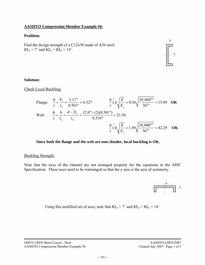
ODOT-LRFD Short Course - Steel AASHTO Compression Member Example #6
AASHTO-LRFD 2007 Created July 2007: Page 1 of 2
AASHTO Compression Member Example #6: Problem: Find the design strength of a C12x30 made of A36 steel. KLy = 7’ and KLx = KLz = 14’. x
y
Solution: Check Local Buckling:
Flange: 3.17" 6.3270.501"
f
f
bbt t= = =
ksi?
ksi
29,0000.56 15.8936y
b Ekt F≤ = = OK
Web: 2 12.0" (2)(0.501") 21.56
0.510"f
w w
d tb ht t t
− −= = = =
ksi?
ksi
29,0001.49 42.2936y
b Ekt F≤ = = OK
Since both the flange and the web are non-slender, local buckling is OK.
Buckling Strength: Note that the axes of the channel are not arranged properly for the equations in the AISC Specification. These axes need to be rearranged so that the y axis is the axis of symmetry.
Using this modified set of axes, note that KLx = 7’ and KLy = KLz = 14’.
-- 121 --

ODOT-LRFD Short Course - Steel AASHTO Compression Member Example #6
AASHTO-LRFD 2007 Created July 2007: Page 2 of 2
Calculate the buckling load for Flexural Buckling about the X-Axis:
( )( ) 22 ksiinft
ksi
7 ' 12 36 1.528(0.762")( ) 29,000
yx
x
FKLr E
⎛ ⎞ ⎛ ⎞⎛ ⎞λ = = =⎜ ⎟ ⎜ ⎟⎜ ⎟π π⎝ ⎠ ⎝ ⎠⎝ ⎠
Since λx < 2.25, Inelastic Buckling Governs
( )( )( )( )1.528 ksi 2 kip0.66 36 8.81 in 167.3nP = = (6.9.4.1-1) Calculate the Critical Stress for Flexural-Torsional Buckling about the Y-axis: For Singly symmetric Sections:
( ) ⎟⎟
⎠
⎞
⎜⎜
⎝
⎛
+−−
+= 2
411
2 ezey
ezeyezeye FF
HFFH
FFF
(AISC E4-5)
2 ksiksi
2inft
( )(29,000 ) 186.6(14 ')(12 )
4.29"
eyF π= =⎛ ⎞⎜ ⎟⎝ ⎠
(AISC E4-10)
( )
2 ksi 6ksi 4
2 2 2inft
ksi
( )(29,000 )(151 in ) 1(11,200 )(0.861 in )(8.81 in )(4.54")(14 ')(12 )
61.54
ez
ez
F
F
⎡ ⎤π= +⎢ ⎥⎢ ⎥⎣ ⎦
=
(AISC E4-11)
ksi ksi ksi ksi
ksi ksi 2
ksi
(186.6 61.54 ) (4)(186.6 )(61.54 )(0.919")1 1(2)(0.919") (186.6 61.54 )
59.30
e
e
F
F
⎛ ⎞⎛ ⎞+= − −⎜ ⎟⎜ ⎟⎜ ⎟+⎝ ⎠⎝ ⎠=
(AISC E4-5)
ksi
ksi
36 0.607159.30
y
e
FF
λ = = =
( )( )( )(0.6071) ksi 2 kip0.66 36 8.81 in 246.0nP = = (6.9.4.1-1)
since 167.3kip < 246.0kip, Flexural Buckling about the x Axis Governs φPn = (0.90)( 167.3kip) = 151kip
-- 122 --

ODOT-LRFD Short Course – Steel AASHTO Compression Member Example #7
AASHTO-LRFD 2007 Created July 2007: Page 1 of 3
AASHTO Compression Members Example #7: Problem: A pair of L4x4x1/2 angles are used as a compression member. The angles are made of M270-36 steel and have an effective length of 12’. The angles are separated by 3/8” thick connectors. Solution: Check Local Buckling:
12
4.0" 8.0"
bt= =
ksi?
ksi
29,0000.45 12.7736y
b Ekt F≤ = =
Local Buckling is OK
Check the Connector Spacing:
( )( )in
ft12 ' 12119.0
(1.21")X
KLr
⎛ ⎞⎛ ⎞ = =⎜ ⎟⎜ ⎟⎝ ⎠ ⎝ ⎠
( )( )in
ft12 ' 1278.69
(1.83")Y
KLr
⎛ ⎞⎛ ⎞ = =⎜ ⎟⎜ ⎟⎝ ⎠ ⎝ ⎠
34i
max
KLa rr
⎛ ⎞⎛ ⎞≤ ⎜ ⎟⎜ ⎟⎝ ⎠⎝ ⎠
( )3(0.776") 119.0 69.26"4
a ⎛ ⎞≤ =⎜ ⎟⎝ ⎠
Use 5 connectors….. a = 36”
ry = 1.83” from AISC 2L Table 1-15, Pg 1-104.
FullyTensioned
4" 3/8" 4"Y
X
-- 123 --

ODOT-LRFD Short Course – Steel AASHTO Compression Member Example #7
AASHTO-LRFD 2007 Created July 2007: Page 2 of 3
Check Flexural Buckling about the X-Axis: (Y axis is the axis of symmetry)
2 2 ksi
ksi
119.0 36 1.78129,000
yX
X
FKLr E
⎛ ⎞⎛ ⎞ ⎛ ⎞λ = = =⎜ ⎟⎜ ⎟ ⎜ ⎟π π⎝ ⎠ ⎝ ⎠ ⎝ ⎠
Since λX < 2.25, Inelastic Buckling Governs ( )( )( )( )1.781 ksi 2 kip0.66 36 7.49 in 127.9nP = = (6.9.4.1-1)
Check Flexural-Torsional Buckling about the Y-Axis: For Tees and Double Angles where the Y axis is the Axis of Symmetry:
( ), , , ,
2, ,
41 1
2cr Y cr Z cr Y cr Z
crft
cr Y cr Z
F F F F HF
H F F
⎛ ⎞+ ⎜ ⎟= − −⎜ ⎟+⎝ ⎠
(AISC E4-2)
Since the section is built-up and the connectors will be in shear for Y-axis buckling, we must consider a modified slenderness ratio…
Calculate Modified Slenderness and Y-axis Flexural Buckling Stress:
22 2
20.82(1 )m o ib
KL KL ar r r
⎛ ⎞α⎛ ⎞ ⎛ ⎞= + ⎜ ⎟⎜ ⎟ ⎜ ⎟ + α⎝ ⎠ ⎝ ⎠ ⎝ ⎠ (6.9.4.3.1-1)
2 ib
hr
α = ( )( ) ( )382 1.18" " 2.735"h = + =
rib = ry for a single angle = 1.21”
2.735" 1.130(2)(1.21")
α = =
( )22
22
(0.82)(1.130) 36"78.69 81.24(1 (1.130) ) 1.21"m
KLr
⎛ ⎞ ⎛ ⎞= + =⎜ ⎟ ⎜ ⎟+⎝ ⎠ ⎝ ⎠
-- 124 --
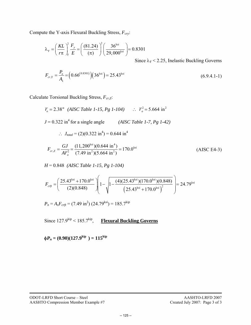
ODOT-LRFD Short Course – Steel AASHTO Compression Member Example #7
AASHTO-LRFD 2007 Created July 2007: Page 3 of 3
Compute the Y-axis Flexural Buckling Stress, Fcry:
22 ksi
ksi
(81.24) 36 0.8301( ) 29,000
yY
Y
FKLr E
⎛ ⎞⎛ ⎞⎛ ⎞λ = = =⎜ ⎟⎜ ⎟⎜ ⎟π π⎝ ⎠ ⎝ ⎠ ⎝ ⎠
Since λY < 2.25, Inelastic Buckling Governs
( )( )( )0.8301 ksi ksi, 0.66 36 25.43n
cr Ys
PFA
= = = (6.9.4.1-1)
Calculate Torsional Buckling Stress, Fcr,Z:
2.38"or = (AISC Table 1-15, Pg 1-104) ∴ 2 25.664 inor =
J = 0.322 in4 for a single angle (AISC Table 1-7, Pg 1-42)
∴ Jtotal = (2)(0.322 in4) = 0.644 in4
ksi 4
ksi, 2 2
(11,200 )(0.644 in ) 170.0(7.49 in )(5.664 in )cr Z
o
GJFAr 2= = = (AISC E4-3)
H = 0.848 (AISC Table 1-15, Pg 1-104)
( )ksi ksi ksi ksi
ksi2ksi ksi
25.43 170.0 (4)(25.43 )(170.0 )(0.848)1 1 24.79(2)(0.848) 25.43 170.0
crftF⎛ ⎞⎛ ⎞+ ⎜ ⎟= − − =⎜ ⎟⎜ ⎟⎜ ⎟⎝ ⎠ +⎝ ⎠
Pn = AsFcrft = (7.49 in2) (24.79ksi) = 185.7kip Since 127.9kip < 185.7kip, Flexural Buckling Governs φPn = (0.90)(127.9kip ) = 115kip
-- 125 --

-- 126 --
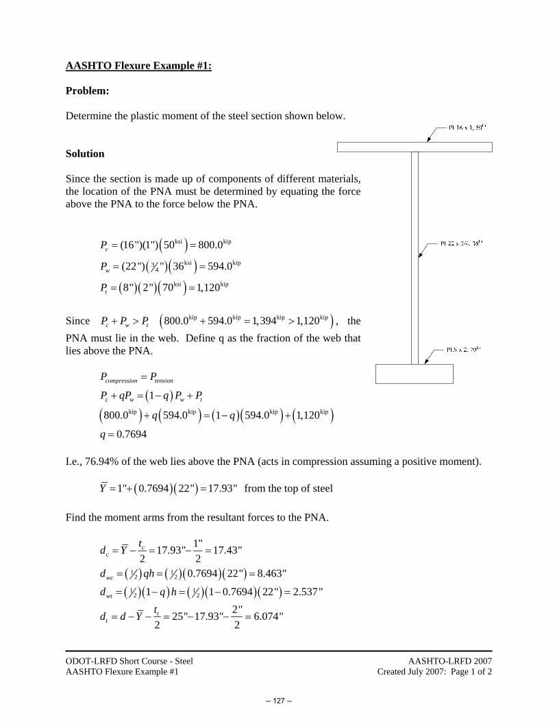
ODOT-LRFD Short Course - Steel AASHTO Flexure Example #1
AASHTO-LRFD 2007 Created July 2007: Page 1 of 2
AASHTO Flexure Example #1: Problem: Determine the plastic moment of the steel section shown below. Solution Since the section is made up of components of different materials, the location of the PNA must be determined by equating the force above the PNA to the force below the PNA.
( )( )( )
( )( )( )
ksi kip
ksi kip34
ksi kip
(16")(1") 50 800.0
(22") " 36 594.0
8" 2" 70 1,120
c
w
t
P
P
P
= =
= =
= =
Since ( )kip kip kip kip 800.0 594.0 1,394 1,120c w tP P P+ > + = > , the PNA must lie in the web. Define q as the fraction of the web that lies above the PNA.
( )
( ) ( ) ( )( ) ( )kip kip kip kip
1
800.0 594.0 1 594.0 1,120
0.7694
compression tension
c w w t
P P
P qP q P P
q q
q
=
+ = − +
+ = − +
=
I.e., 76.94% of the web lies above the PNA (acts in compression assuming a positive moment).
( )( )1" 0.7694 22" 17.93"Y = + = from the top of steel
Find the moment arms from the resultant forces to the PNA.
( ) ( )( )( )( )( ) ( )( )( )
1 12 2
1 12 2
1"17.93" 17.43"2 2
0.7694 22" 8.463"
1 1 0.7694 22" 2.537"2"25" 17.93" 6.074"
2 2
cc
wc
wt
tt
td Y
d qh
d q htd d Y
= − = − =
= = =
= − = − =
= − − = − − =
-- 127 --
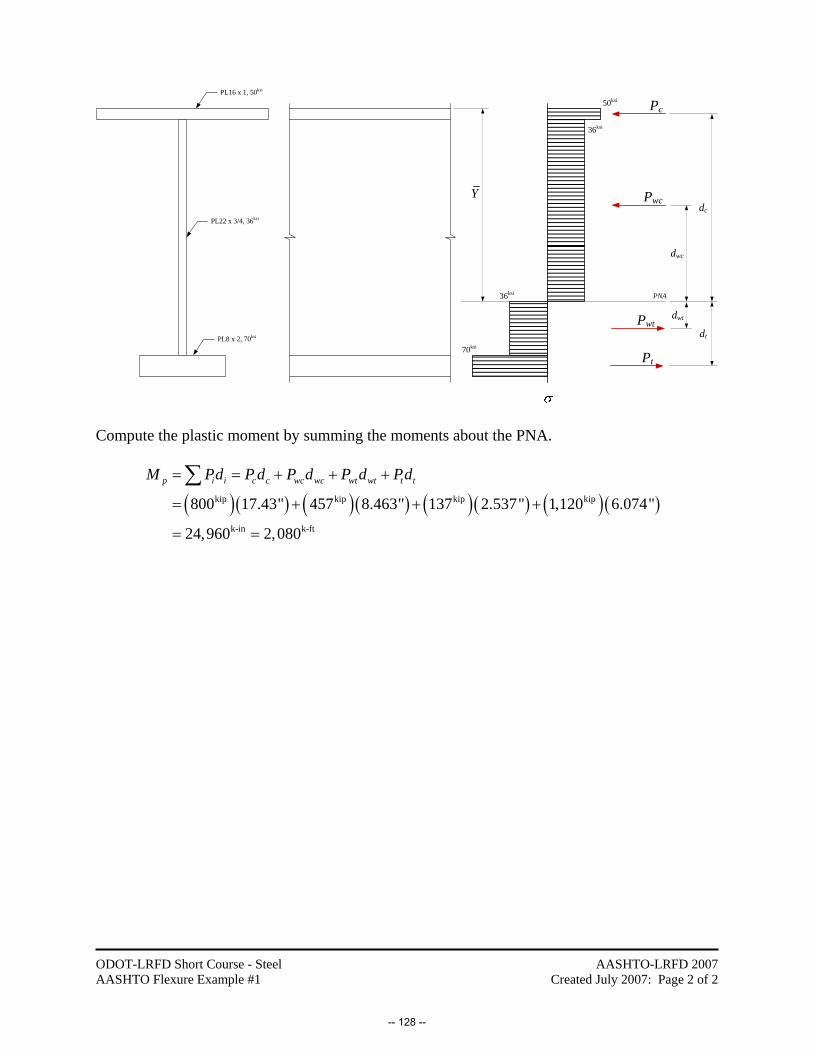
ODOT-LRFD Short Course - Steel AASHTO Flexure Example #1
AASHTO-LRFD 2007 Created July 2007: Page 2 of 2
PL16 x 1, 50ksi
PL22 x 3/4, 36ksi
PL8 x 2, 70ksi
Pc
Pwt
dwc
PNA
50ksi
dcPwc
Pt
dwt
dt
36ksi
36ksi
70ksi
Y
Compute the plastic moment by summing the moments about the PNA.
( )( ) ( )( ) ( )( ) ( )( )kip kip kip kip
k-in k-ft
800 17.43" 457 8.463" 137 2.537" 1,120 6.074"
24,960 2,080
p i i c c wc wc wt wt t tM Pd P d P d P d Pd= = + + +
= + + +
= =
∑
-- 128 --
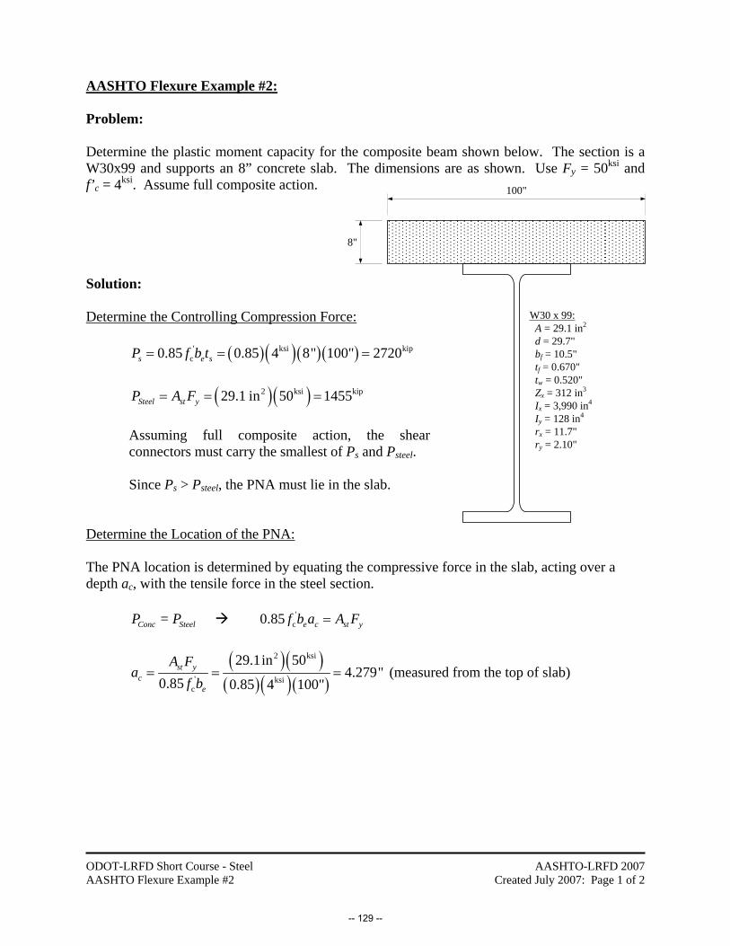
ODOT-LRFD Short Course - Steel AASHTO Flexure Example #2
AASHTO-LRFD 2007 Created July 2007: Page 1 of 2
AASHTO Flexure Example #2: Problem: Determine the plastic moment capacity for the composite beam shown below. The section is a W30x99 and supports an 8” concrete slab. The dimensions are as shown. Use Fy = 50ksi and f’c = 4ksi. Assume full composite action.
Solution:
Determine the Controlling Compression Force:
( )( )( )( )' ksi kipc0.85 0.85 4 8" 100" 2720s e sP f b t= = =
( )( )2 ksi kip29.1 in 50 1455Steel st yP A F= = =
Assuming full composite action, the shear connectors must carry the smallest of Ps and Psteel. Since Ps > Psteel, the PNA must lie in the slab.
Determine the Location of the PNA:
The PNA location is determined by equating the compressive force in the slab, acting over a depth ac, with the tensile force in the steel section.
=Conc SteelP P '
c0.85 e c st yf b a A F=
( )( )( )( )( )
2 ksi
' ksic
29.1 in 504.279"
0.85 0.85 4 100"st y
ce
A Fa
f b= = = (measured from the top of slab)
100"
8"
W30 x 99:A = 29.1 in2
d = 29.7" bf = 10.5" tf = 0.670" tw = 0.520" Zx = 312 in3
Ix = 3,990 in4
Iy = 128 in4
rx = 11.7" ry = 2.10"
-- 129 --

ODOT-LRFD Short Course - Steel AASHTO Flexure Example #2
AASHTO-LRFD 2007 Created July 2007: Page 2 of 2
Determine the Plastic Moment:
The plastic moment is calculated by summing the tension and compression forces about any point. In general, the moments are summed about the PNA. In this case (where the PNA is in the slab) it is simplest to sum moments about either force PSteel or the force Pconc. Note that the tension force in the concrete is ignored.
100"
8"Pconc
Psteel
a1
PNA
0.85f’c
Fy
ac
( ) ( )1 1( ) ( )p Conc SteelM P a P a= =
129.7" 4.279"8" 20.71"
2 2 2 2st c
sd aa t= + − = + − =
( )kip k-in k-ft1455 (20.71") 30,130 2,511pM = = =
-- 130 --

ODOT-LRFD Short Course - Steel AASHTO Flexure Example #3
AASHTO-LRFD 2007 Created July 2007: Page 1 of 3
AASHTO Flexure Example #3: Problem: Determine the plastic moment capacity for the composite beam shown below. The section is a W30x99 and supports a 6” thick concrete slab. The dimensions are as shown. Use Fy = 50ksi and f’c = 4ksi. Assume full composite action. Solution: Determine the Controlling Compression Force:
( )( )( )( )' ksi kip
c0.85 0.85 4 6" 50" 1020s s sP f b t= = =
( )( )2 ksi kip29.1 in 50 1455Steel st yP A F= = =
Assuming full composite action, the shear connectors must carry the smallest of Ps and Psteel. Since Ps < Psteel, the PNA must lie in the steel. When this occurs, it is simplest to use the aids in Appendix D of the AASHTO Specification to determine the location of the PNA and plastic moment.
Referring to Table D6.1-1 in Appendix D6.1, Page 6-290:
Determine the forces in the components of the cross section. The forces in the rebar will be conservatively taken as zero (we don’t know what size the rebar is any ways…)
( )( )( )( )
( )( )
' ksi kipc
ksi kip
2 ksi kip
kip
0.85 0.85 4 6" 50" 1020
(0.670")(10.5") 50 351.8
29.1 in (2)(0.670")(10.5") 50 751.5
351.8
s s s
c
w
t c
P f b t
P
P
P P
= = =
= =
⎡ ⎤= − =⎣ ⎦= =
Check Case I ?
t w c sP P P P+ ≥ +
?
kip kip kip kip351.8 751.5 351.8 1020+ ≥ + NO
In this case, I took Aw = Asteel - 2Af. Otherwise, Pc+Pt+Pw ≠ Psteel. If you take Aw = D tw where D = d - 2tf, the plastic moment changes by ~2%
-- 131 --

ODOT-LRFD Short Course - Steel AASHTO Flexure Example #3
AASHTO-LRFD 2007 Created July 2007: Page 2 of 3
Check Case II ?
t w c sP P P P+ + ≥
?
kip kip kip kip351.8 751.5 351.8 1020+ + ≥ YES - PNA in Top Flange
50"
6"Ps
Pw
ds PNA
0.85f’c
FyPt
Fy
dw
dt
Pc2
Pc1
First, the location of the PNA within the top flange is determined.
kip kip kip
kip
12
0.670" 751.5 351.8 1,020 1 0.2368"2 351.8
c w t s
c
t P P PYP
⎛ ⎞+ −⎛ ⎞= +⎜ ⎟⎜ ⎟⎝ ⎠⎝ ⎠
⎛ ⎞+ −⎛ ⎞= + =⎜ ⎟⎜ ⎟⎝ ⎠⎝ ⎠
Next, the distances from the component forces to the PNA are calculated.
6" 0.2368" 3.237"229.7" 0.2368" 14.61"
20.670"29.7" 0.2368" 29.13"
2
s
w
t
d
d
d
= + =
= − =
= − − =
-- 132 --

ODOT-LRFD Short Course - Steel AASHTO Flexure Example #3
AASHTO-LRFD 2007 Created July 2007: Page 3 of 3
Finally, the plastic moment is computed.
( ) [ ]
( ) ( )
( )( ) ( )( ) ( )( )
( )
22
kip2 2
kip kip kip
kip 2 k-inin
k-
2
351.8 0.2368" 0.670" 0.2368" ...(2)(0.670")
... 1,020 3.237" 751.5 14.61" 351.8 29.13"
262.5 0.2437 in 24,530
24,590
cp c s s w w t t
c
PM Y t Y P d P d Pdt
⎛ ⎞ ⎡ ⎤= + − + + +⎜ ⎟ ⎣ ⎦⎝ ⎠⎛ ⎞ ⎡ ⎤= + − +⎜ ⎟ ⎣ ⎦⎝ ⎠
⎡ ⎤+ + +⎣ ⎦
⎡ ⎤ ⎡ ⎤= +⎣ ⎦ ⎣ ⎦
= in k-ft2,049=
-- 133 --
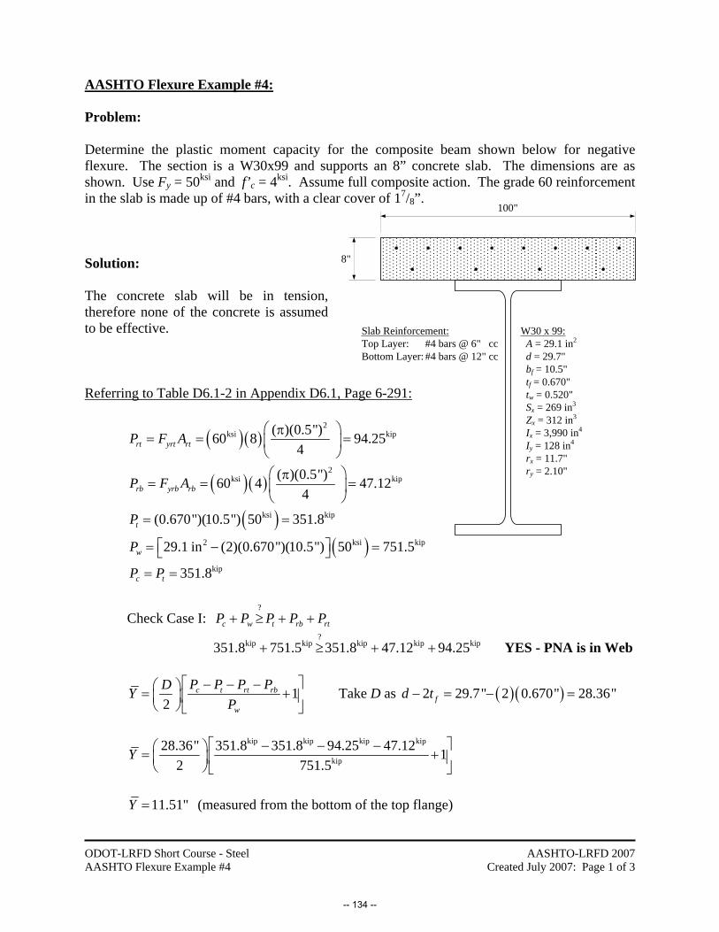
ODOT-LRFD Short Course - Steel AASHTO Flexure Example #4
AASHTO-LRFD 2007 Created July 2007: Page 1 of 3
AASHTO Flexure Example #4: Problem: Determine the plastic moment capacity for the composite beam shown below for negative flexure. The section is a W30x99 and supports an 8” concrete slab. The dimensions are as shown. Use Fy = 50ksi and f’c = 4ksi. Assume full composite action. The grade 60 reinforcement in the slab is made up of #4 bars, with a clear cover of 17/8”.
Solution: The concrete slab will be in tension, therefore none of the concrete is assumed to be effective. Referring to Table D6.1-2 in Appendix D6.1, Page 6-291:
( )( )2
ksi kip( )(0.5")60 8 94.254rt yrt rtP F A
⎛ ⎞π= = =⎜ ⎟
⎝ ⎠
( )( )2
ksi kip( )(0.5")60 4 47.124rb yrb rbP F A
⎛ ⎞π= = =⎜ ⎟
⎝ ⎠
( )( )
ksi kip
2 ksi kip
kip
(0.670")(10.5") 50 351.8
29.1 in (2)(0.670")(10.5") 50 751.5
351.8
t
w
c t
P
P
P P
= =
⎡ ⎤= − =⎣ ⎦= =
Check Case I: ?
c w t rb rtP P P P P+ ≥ + +
?
kip kip kip kip kip351.8 751.5 351.8 47.12 94.25+ ≥ + + YES - PNA is in Web
12
c t rt rb
w
P P P PDYP
⎡ ⎤− − −⎛ ⎞= +⎢ ⎥⎜ ⎟⎝ ⎠ ⎣ ⎦
Take D as ( )( )2 29.7" 2 0.670" 28.36"fd t− = − =
kip kip kip kip
kip
28.36" 351.8 351.8 94.25 47.12 12 751.5
Y⎡ ⎤− − −⎛ ⎞= +⎜ ⎟ ⎢ ⎥
⎝ ⎠ ⎣ ⎦
11.51"Y = (measured from the bottom of the top flange)
100"
8"
W30 x 99:A = 29.1 in2
d = 29.7" bf = 10.5" tf = 0.670" tw = 0.520" Sx = 269 in3
Zx = 312 in3
Ix = 3,990 in4
Iy = 128 in4
rx = 11.7" ry = 2.10"
Slab Reinforcement:Top Layer: #4 bars @ 6" ccBottom Layer: #4 bars @ 12" cc
-- 134 --

ODOT-LRFD Short Course - Steel AASHTO Flexure Example #4
AASHTO-LRFD 2007 Created July 2007: Page 2 of 3
( )( )7 1 1
8 2 211.51" 0.670" 8" 1 " " 18.06"rtd = + + − + =⎡ ⎤⎣ ⎦
( )( )7 1 18 2 211.51" 0.670" 1 " " 14.31"rbd = + + + =⎡ ⎤⎣ ⎦
( )( )1211.51" 0.670" 11.85"td = + =
( )( )12 11.51" 5.755"wtd = =
( )( )12 28.36" 11.51" 8.425"wcd = − =
( ) ( )( )1228.36" 11.51" 0.670" 17.19"cd = − + =
[ ]2 2( )2
wp rt rt rb rb t t c c
PM y D y P d P d Pd P dD
⎛ ⎞ ⎡ ⎤= + − + + + +⎜ ⎟ ⎣ ⎦⎝ ⎠
kip2 2 kip
kip kip kip
751.5 (11.51") (28.36" 11.51") [(94.25 )(18.06") ...(2)(28.36")
... (47.12 )(14.31") (351.8 )(11.85") (351.8 )(17.19")]
⎡ ⎤= + − + +⎣ ⎦
+ + +
k-in k-ft18,110 1,509= =
Not needed when using Table D6.1-2
-- 135 --
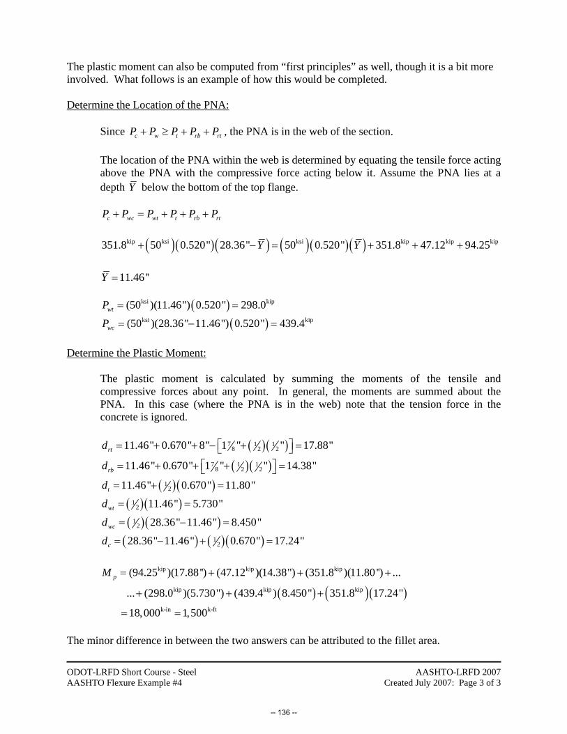
ODOT-LRFD Short Course - Steel AASHTO Flexure Example #4
AASHTO-LRFD 2007 Created July 2007: Page 3 of 3
The plastic moment can also be computed from “first principles” as well, though it is a bit more involved. What follows is an example of how this would be completed. Determine the Location of the PNA:
Since c w t rb rtP P P P P+ ≥ + + , the PNA is in the web of the section. The location of the PNA within the web is determined by equating the tensile force acting above the PNA with the compressive force acting below it. Assume the PNA lies at a depth Y below the bottom of the top flange.
c wc wt t rb rtP P P P P P+ = + + +
( )( )( ) ( )( )( )kip ksi ksi kip kip kip351.8 50 0.520" 28.36" 50 0.520" 351.8 47.12 94.25Y Y+ − = + + +
11.46 ''Y =
( )ksi kip(50 )(11.46") 0.520" 298.0wtP = =
( )ksi kip(50 )(28.36" 11.46") 0.520" 439.4wcP = − = Determine the Plastic Moment:
The plastic moment is calculated by summing the moments of the tensile and compressive forces about any point. In general, the moments are summed about the PNA. In this case (where the PNA is in the web) note that the tension force in the concrete is ignored.
( )( )7 1 18 2 211.46" 0.670" 8" 1 " " 17.88"rtd = + + − + =⎡ ⎤⎣ ⎦
( )( )7 1 18 2 211.46" 0.670" 1 " " 14.38"rbd = + + + =⎡ ⎤⎣ ⎦
( )( )1211.46" 0.670" 11.80"td = + =
( )( )12 11.46" 5.730"wtd = =
( )( )12 28.36" 11.46" 8.450"wcd = − =
( ) ( )( )1228.36" 11.46" 0.670" 17.24"cd = − + =
( ) ( )( )
kip kip kip
kip kip kip
(94.25 )(17.88'') (47.12 )(14.38") (351.8 )(11.80 '') ...
... (298.0 )(5.730") (439.4 ) 8.450" 351.8 17.24"pM = + + +
+ + +
k-in k-ft18,000 1,500= = The minor difference in between the two answers can be attributed to the fillet area.
-- 136 --

ODOT-LRFD Short Course - Steel AASHTO Flexure Example #5a
AASHTO-LRFD 2007 Created July 2007: Page 1 of 4
AASHTO Flexural Example #5a: Problem: A non-composite W30x99 made of M270-50 steel is used to span 48’. The beam is braced laterally at 12’-0” intervals and is subjected to a factored load of w = 3.75kip/ft, which includes the self weight of the beam. Check to see if the section is adequate considering flexural failure modes at the Strength Limit States. If appropriate, use the provisions in AASHTO Section 6.10.8 to determine capacity. Solution:
Determine Classification of the Section:
Check ?2 5.7c
w yc
D Et F
≤ (6.10.6.2.3-1)
Take D = d - 2tf = 29.7” - (2)(0.670”) = 28.36”
28.36" 14.18"2 2cDD = = =
ksi?
ksi
(2)(14.18") 29,00054.54 5.7 137.3(0.520") 50
= ≤ = OK, ∴ web is non-slender
Check ?
0.3yc
yt
II
≥ (6.10.6.2.3-2)
Since Section is doubly symmetric, Iyc = Iyt OK
-- 137 --
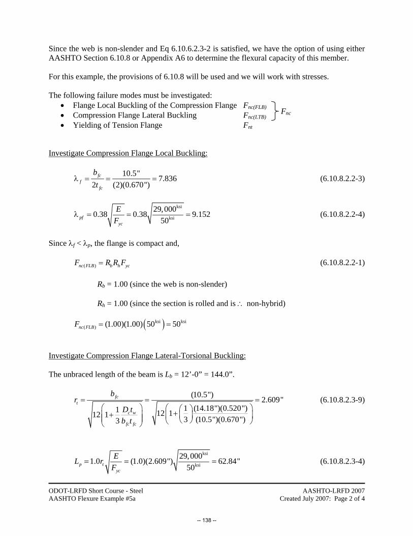
ODOT-LRFD Short Course - Steel AASHTO Flexure Example #5a
AASHTO-LRFD 2007 Created July 2007: Page 2 of 4
Since the web is non-slender and Eq 6.10.6.2.3-2 is satisfied, we have the option of using either AASHTO Section 6.10.8 or Appendix A6 to determine the flexural capacity of this member. For this example, the provisions of 6.10.8 will be used and we will work with stresses. The following failure modes must be investigated:
• Flange Local Buckling of the Compression Flange Fnc(FLB) • Compression Flange Lateral Buckling Fnc(LTB) • Yielding of Tension Flange Fnt
Investigate Compression Flange Local Buckling:
10.5" 7.8362 (2)(0.670")
fcf
fc
bt
λ = = = (6.10.8.2.2-3)
ksi
ksi
29,0000.38 0.38 9.15250pf
yc
EF
λ = = = (6.10.8.2.2-4)
Since λf < λp, the flange is compact and, ( )nc FLB b h ycF R R F= (6.10.8.2.2-1) Rb = 1.00 (since the web is non-slender) Rh = 1.00 (since the section is rolled and is ∴ non-hybrid) ( )ksi ksi
( ) (1.00)(1.00) 50 50nc FLBF = = Investigate Compression Flange Lateral-Torsional Buckling: The unbraced length of the beam is Lb = 12’-0” = 144.0”.
(10.5") 2.609"1 (14.18")(0.520")1 12 112 1 3 (10.5")(0.670")3
fct
c w
fc fc
br
D tb t
= = =⎛ ⎞ ⎛ ⎞⎛ ⎞++ ⎜ ⎟⎜ ⎟ ⎜ ⎟⎜ ⎟ ⎝ ⎠⎝ ⎠⎝ ⎠
(6.10.8.2.3-9)
ksi
ksi
29,0001.0 (1.0)(2.609") 62.84"50p t
yc
EL rF
= = = (6.10.8.2.3-4)
Fnc
-- 138 --
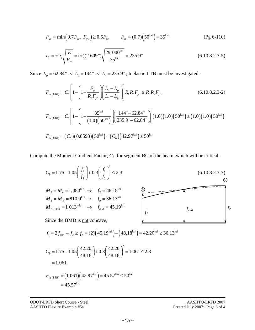
ODOT-LRFD Short Course - Steel AASHTO Flexure Example #5a
AASHTO-LRFD 2007 Created July 2007: Page 3 of 4
( )min 0.7 , 0.5yr yc yw ycF F F F= ≥ ( )ksi ksi(0.7) 50 35yrF = = (Pg 6-110)
ksi
ksi
29,000 ( )(2.609") 235.9"35r t
yr
EL rF
= π = π = (6.10.8.2.3-5)
Since 62.84" 144" 235.9"p b rL L L= < = < = , Inelastic LTB must be investigated.
( ) 1 1 yr b pnc LTB b b h yc b h yc
h yc r p
F L LF C R R F R R F
R F L L
⎡ ⎤⎛ ⎞⎛ ⎞−= − − ≤⎢ ⎥⎜ ⎟⎜ ⎟⎜ ⎟⎜ ⎟−⎢ ⎥⎝ ⎠⎝ ⎠⎣ ⎦
(6.10.8.2.3-2)
( )( ) ( )( )( ) ( )( )( )
ksiksi ksi
( ) ksi
35 144" 62.84"1 1 1.0 1.0 50 1.0 1.0 50235.9" 62.84"1.0 50nc LTB bF C
⎡ ⎤⎛ ⎞ −⎛ ⎞⎢ ⎥⎜ ⎟= − − ≤⎜ ⎟⎜ ⎟ −⎢ ⎥⎝ ⎠⎝ ⎠⎣ ⎦
( )( )( ) ( )( )ksi ksi ksi
( ) 0.8593 50 42.97 50nc LTB b bF C C= = ≤ Compute the Moment Gradient Factor, Cb, for segment BC of the beam, which will be critical.
2
1 1
2 2
1.75 1.05 0.3 2.3bf fCf f
⎛ ⎞ ⎛ ⎞= − + ≤⎜ ⎟ ⎜ ⎟
⎝ ⎠ ⎝ ⎠ (6.10.8.2.3-7)
k-ft ksi2 2
k-ft ksi
k-ft ksi,
1,080 48.18
810.0 36.13
1,013 45.19
c
o B o
BC mid mid
M M f
M M f
M f
= = → =
= = → =
= → =
Since the BMD is not concave, ( ) ( )ksi ksi ksi ksi
1 22 (2) 45.19 48.18 42.20 36.13mid of f f f= − ≥ = − = ≥
242.20 42.201.75 1.05 0.3 1.061 2.348.18 48.18
1.061
bC ⎛ ⎞ ⎛ ⎞= − + = ≤⎜ ⎟ ⎜ ⎟⎝ ⎠ ⎝ ⎠
=
( )( )ksi ksi ksi( )
ksi
1.061 42.97 45.57 50
45.57nc LTBF = = ≤
=
B
C
f2fmidf1
-- 139 --

ODOT-LRFD Short Course - Steel AASHTO Flexure Example #5a
AASHTO-LRFD 2007 Created July 2007: Page 4 of 4
The governing strength for the compression flange is the smaller of Fnc(FLB) and Fnc(LTB):
Since ksi ksi( ) ( )45.57 50.00nc LTB nc FLBF F= < = , LTB governs the strength of the
compression flange.
ksi( ) 45.57nc nc LTBF F= =
( )ksi ksi(1.00) 45.57 45.57ncFφ = =
Check 13bu l f ncf f F+ ≤ φ (6.10.8.1.1-1)
ksi48.18bu Cf f= = Assume that Strength I Load Combination Governs, ∴ γWS = 0.0 and fl = 0
Since ksi ksi1 48.18 =45.573bu l f ncf f F+ = > φ , the compression flange is not adequate.
Investigate the Strength of the Tension Flange: Since the tension flange is discretely braced, ( )ksi ksi(1.0) 50 50nt h ytF R F= = = (6.10.8.3-1) ( )ksi ksi(1.00) 50 50ntFφ = =
Check 13bu l f ntf f F+ ≤ φ (6.10.8.1.2-1)
ksi48.18bu Cf f= =
Since ksi ksi1 48.18 =50.003bu l f ntf f F+ = < φ , the tension flange is adequate.
Since the compression flange is not adequate, the section is not adequate for flexure.
-- 140 --
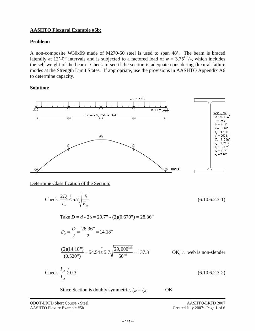
ODOT-LRFD Short Course - Steel AASHTO Flexure Example #5b
AASHTO-LRFD 2007 Created July 2007: Page 1 of 6
AASHTO Flexural Example #5b: Problem: A non-composite W30x99 made of M270-50 steel is used to span 48’. The beam is braced laterally at 12’-0” intervals and is subjected to a factored load of w = 3.75kip/ft, which includes the self weight of the beam. Check to see if the section is adequate considering flexural failure modes at the Strength Limit States. If appropriate, use the provisions in AASHTO Appendix A6 to determine capacity. Solution:
Determine Classification of the Section:
Check ?2 5.7c
w yc
D Et F
≤ (6.10.6.2.3-1)
Take D = d - 2tf = 29.7” - (2)(0.670”) = 28.36”
28.36" 14.18"2 2cDD = = =
ksi?
ksi
(2)(14.18") 29,00054.54 5.7 137.3(0.520") 50
= ≤ = OK, ∴ web is non-slender
Check ?
0.3yc
yt
II
≥ (6.10.6.2.3-2)
Since Section is doubly symmetric, Iyc = Iyt OK
-- 141 --

ODOT-LRFD Short Course - Steel AASHTO Flexure Example #5b
AASHTO-LRFD 2007 Created July 2007: Page 2 of 6
Since the web is non-slender and Eq 6.10.6.2.3-2 is satisfied, we have the option of using either AASHTO Section 6.10.8 or Appendix A6 to determine the flexural capacity of this member. For this example, the provisions of A6 will be used and we will work with moments. The following failure modes must be investigated:
• Flange Local Buckling of the Compression Flange Mnc(FLB) • Lateral-Torsional Buckling Mnc(LTB) • Yielding of Tension Flange Mnt
Compute Web Plasticity Factors, Rpc and Rpt (Section A6.2): Investigate the classification of the web.
Check ?
( )
2cp
cppw D
w
Dt
≤λ (A6.2.1-1)
( ) 20.54
0.09cp
yc cppw D rw
cp
h y
EF D
DMR M
⎛ ⎞λ = ≤ λ ⎜ ⎟
⎛ ⎞ ⎝ ⎠−⎜ ⎟⎜ ⎟
⎝ ⎠
(A6.2.1-2)
5.7 137.3rwyc
EF
λ = = (A6.2.1-3)
Rh = 1.00 (since the section is rolled and is ∴ non-hybrid)
( )( )( )( )
3 ksi k-in k-ft
3 ksi k-in k-ft
269 in 50 13,450 1,121
312 in 50 15,600 1,300
y x y
p x y
M S F
M Z F
= = = =
= = = =
( )( )( )( )
ksi
ksi
( ) 2k-in
k-in
29,00014.18"50 83.76 137.3 137.314.18"0.54 15,600
0.091.0 13,450
cppw D⎛ ⎞λ = = ≤ =⎜ ⎟⎝ ⎠⎛ ⎞
⎜ ⎟−⎜ ⎟⎝ ⎠
( ) 83.76
cppw Dλ =
Mnc
-- 142 --
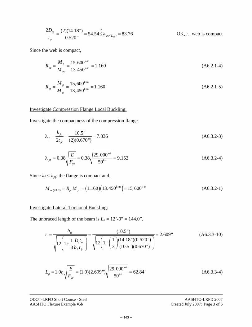
ODOT-LRFD Short Course - Steel AASHTO Flexure Example #5b
AASHTO-LRFD 2007 Created July 2007: Page 3 of 6
?
( )
2 (2)(14.18") 54.54 83.760.520" cp
cppw D
w
Dt
= = ≤λ = OK, ∴ web is compact
Since the web is compact,
k-in
k-in
15,600 1.16013,450
ppc
yc
MR
M= = = (A6.2.1-4)
k-in
k-in
15,600 1.16013,450
ppt
yt
MR
M= = = (A6.2.1-5)
Investigate Compression Flange Local Buckling: Investigate the compactness of the compression flange.
10.5" 7.8362 (2)(0.670")
fcf
fc
bt
λ = = = (A6.3.2-3)
ksi
ksi
29,0000.38 0.38 9.15250pf
yc
EF
λ = = = (A6.3.2-4)
Since λf < λpf, the flange is compact and, ( )( )k-in k-in
( ) 1.160 13,450 15,600nc FLB pc ycM R M= = = (A6.3.2-1) Investigate Lateral-Torsional Buckling: The unbraced length of the beam is Lb = 12’-0” = 144.0”.
(10.5") 2.609"1 (14.18")(0.520")1 12 112 1 3 (10.5")(0.670")3
fct
c w
fc fc
br
D tb t
= = =⎛ ⎞ ⎛ ⎞⎛ ⎞++ ⎜ ⎟⎜ ⎟ ⎜ ⎟⎜ ⎟ ⎝ ⎠⎝ ⎠⎝ ⎠
(A6.3.3-10)
ksi
ksi
29,0001.0 (1.0)(2.609") 62.84"50p t
yc
EL rF
= = = (A6.3.3-4)
-- 143 --
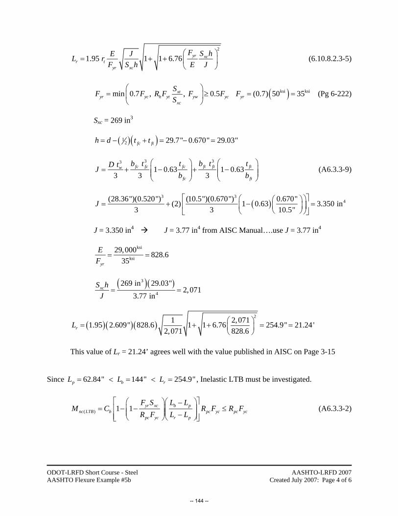
ODOT-LRFD Short Course - Steel AASHTO Flexure Example #5b
AASHTO-LRFD 2007 Created July 2007: Page 4 of 6
2
1.95 1 1 6.76 yr xcr t
yr xc
F S hE JL rF S h E J
⎛ ⎞= + + ⎜ ⎟
⎝ ⎠ (6.10.8.2.3-5)
min 0.7 , , 0.5xtyr yc h yt yw yc
xc
SF F R F F FS
⎛ ⎞= ≥⎜ ⎟
⎝ ⎠ ( )ksi ksi(0.7) 50 35yrF = = (Pg 6-222)
Sxc = 269 in3 ( )( )1
2 29.7" 0.670" 29.03"fc fth d t t= − + = − =
3 33 1 0.63 1 0.63
3 3 3fc fc fc ft ft ftw
fc ft
b t t b t tD tJb b
⎛ ⎞ ⎛ ⎞= + − + −⎜ ⎟ ⎜ ⎟⎜ ⎟ ⎜ ⎟
⎝ ⎠ ⎝ ⎠ (A6.3.3-9)
( )3 3
4(28.36")(0.520") (10.5")(0.670") 0.670"(2) 1 0.63 3.350 in3 3 10.5"
J⎡ ⎤⎛ ⎞⎛ ⎞= + − =⎢ ⎥⎜ ⎟⎜ ⎟⎝ ⎠⎝ ⎠⎣ ⎦
J = 3.350 in4 J = 3.77 in4 from AISC Manual….use J = 3.77 in4
ksi
ksi
29,000 828.635yr
EF
= =
( )( )3
4
269 in 29.03"2,071
3.77 inxcS hJ
= =
( )( )( )21 2,0711.95 2.609" 828.6 1 1 6.76 254.9" 21.24 '
2,071 828.6rL ⎛ ⎞= + + = =⎜ ⎟⎝ ⎠
This value of Lr = 21.24’ agrees well with the value published in AISC on Page 3-15 Since 62.84" 144" 254.9"p b rL L L= < = < = , Inelastic LTB must be investigated.
( ) 1 1 yr xc b pnc LTB b pc yc pc yc
pc yc r p
F S L LM C R F R F
R F L L
⎡ ⎤⎛ ⎞⎛ ⎞−= − − ≤⎢ ⎥⎜ ⎟⎜ ⎟⎜ ⎟⎜ ⎟−⎢ ⎥⎝ ⎠⎝ ⎠⎣ ⎦
(A6.3.3-2)
-- 144 --

ODOT-LRFD Short Course - Steel AASHTO Flexure Example #5b
AASHTO-LRFD 2007 Created July 2007: Page 5 of 6
( )( )( )( ) ( )( ) ( )( )
( )( )( ) ( )( )
ksi 3k-in k-in
( ) k-in
k-in k-in k-in
35 269 in 144" 62.84"1 1 1.160 13,450 1.160 13,450254.9" 62.84"1.16 13,450
0.9656 15,600 12,990 15,600
nc LTB b
b b
M C
C C
⎡ ⎤⎛ ⎞ −⎛ ⎞⎢ ⎥⎜ ⎟= − − ≤⎜ ⎟⎜ ⎟ −⎢ ⎥⎝ ⎠⎝ ⎠⎣ ⎦
= = ≤
Compute the Moment Gradient Factor, Cb, for segment BC of the beam, which will be critical.
2
1 1
2 2
1.75 1.05 0.3 2.3bM MCM M
⎛ ⎞ ⎛ ⎞= − + ≤⎜ ⎟ ⎜ ⎟
⎝ ⎠ ⎝ ⎠ (A6.3.3-7)
k-ft2
k-ft
k-ft,
1,080
810.0
1,013
c
o B
BC mid
M M
M M
M
= =
= =
=
Since the BMD is not concave, ( ) ( )k-ft k-ft k-ft k-ft
1 22 (2) 1,013 1,080 946 810mid oM M M M= − ≥ = − = ≥
2946 9461.75 1.05 0.3 1.061 2.31,080 1,080
1.061
bC ⎛ ⎞ ⎛ ⎞= − + = ≤⎜ ⎟ ⎜ ⎟⎝ ⎠ ⎝ ⎠
=
( )( )k-in k-in k-in
( ) 1.061 12,990 13,780 15,600nc LTBM = = ≤ k-in
( ) 13,780nc LTBM =
-- 145 --

ODOT-LRFD Short Course - Steel AASHTO Flexure Example #5b
AASHTO-LRFD 2007 Created July 2007: Page 6 of 6
The governing strength for the compression flange is the smaller of Mnc(FLB) and Mnc(LTB):
Since k-in k-in( ) ( )13,780 15,600nc LTB nc FLBM M= < = , LTB governs the strength of the
compression flange.
k-in k-ft( ) 13,780 1,148nc nc LTBM M= = =
( )k-ft k-ft(1.00) 1,148 1,148ncMφ = =
Check 13u l xc f ncM f S M+ ≤ φ (A6.1.1-1)
k-ft1,080u CM M= = Assume that Strength I Load Combination Governs, ∴ γWS = 0.0 and fl = 0
Since k-ft k-ft1 1,080 =1,1483u l xc f ncM f S M+ = < φ , the compression flange is adequate.
Investigate the Strength of the Tension Flange: Since the tension flange is discretely braced, ( )k-in k-in k-ft(1.160) 13,450 15,600 1,300nt pt ytM R M= = = = (A6.4-1) ( )k-ft k-ft(1.00) 1,300 1,300ntMφ = =
Check 13u l xt f ntM f S M+ ≤ φ (6.10.8.1.2-1)
k-ft1,080u CM M= =
Since k-ft k-ft1 1,080 =1,3003u l xt f ntM f S M+ = < φ , the tension flange is adequate.
Since both flanges are adequate, the section is adequate for flexure.
Note that the benefits of using Appendix A6 are illustrated here since the section was found to be not adequate when the provisions in Section 6.10.8 were used to compute capacity.
-- 146 --

ODOT-LRFD Short Course - Steel AASHTO Flexure Example #6a
AASHTO-LRFD 2007 Created July 2007: Page 1 of 5
AASHTO Flexural Example #6a: Problem: A non-composite built-up girder made of M270-50 steel is used to span 48’. The beam is braced laterally at 12’-0” intervals and is subjected to a factored load of w = 3.75kip/ft, which includes the self weight of the beam. Check to see if the section is adequate considering flexural failure modes at the Strength Limit States. If appropriate, use the provisions in AASHTO Section 6.10.8 to determine capacity. Solution:
Determine Classification of the Section:
Check ?2 5.7c
w yc
D Et F
≤ (6.10.6.2.3-1)
Take D = 38”
38" 19"2 2cDD = = =
ksi?
ksi38
(2)(19") 29,000101.3 5.7 137.3( ") 50
= ≤ = OK, ∴ web is non-slender
Check ?
0.3yc
yt
II
≥ (6.10.6.2.3-2)
Since Section is doubly symmetric, Iyc = Iyt OK
PL16 x 3/4
PL38 x 3/8
PL16 x 3/4
Ix = 10,730 in4
Iy = 513.2 in4
Sx = 543.1 in3
Sy = 64.15 in3
-- 147 --
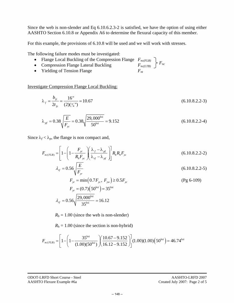
ODOT-LRFD Short Course - Steel AASHTO Flexure Example #6a
AASHTO-LRFD 2007 Created July 2007: Page 2 of 5
Since the web is non-slender and Eq 6.10.6.2.3-2 is satisfied, we have the option of using either AASHTO Section 6.10.8 or Appendix A6 to determine the flexural capacity of this member. For this example, the provisions of 6.10.8 will be used and we will work with stresses. The following failure modes must be investigated:
• Flange Local Buckling of the Compression Flange Fnc(FLB) • Compression Flange Lateral Buckling Fnc(LTB) • Yielding of Tension Flange Fnt
Investigate Compression Flange Local Buckling:
3
4
16" 10.672 (2)( ")
fcf
fc
bt
λ = = = (6.10.8.2.2-3)
ksi
ksi
29,0000.38 0.38 9.15250pf
yc
EF
λ = = = (6.10.8.2.2-4)
Since λf < λp, the flange is non compact and,
( ) 1 1 yr f pfnc FLB b h yc
h yc rf pf
FF R R F
R F
⎡ ⎤⎛ ⎞⎛ ⎞λ −λ= − −⎢ ⎥⎜ ⎟⎜ ⎟⎜ ⎟⎜ ⎟λ −λ⎢ ⎥⎝ ⎠⎝ ⎠⎣ ⎦
(6.10.8.2.2-2)
0.56rfyr
EF
λ = (6.10.8.2.2-5)
( )min 0.7 , 0.5yr yc yw ycF F F F= ≥ (Pg 6-109)
( )ksi ksi(0.7) 50 35yrF = =
ksi
ksi
29,0000.56 16.1235rf = =λ
Rb = 1.00 (since the web is non-slender) Rh = 1.00 (since the section is non-hybrid)
( )ksi
ksi ksi( ) ksi
35 10.67 9.1521 1 (1.00)(1.00) 50 46.74(1.00)(50 ) 16.12 9.152nc FLBF
⎡ ⎤⎛ ⎞ −⎛ ⎞= − − =⎢ ⎥⎜ ⎟⎜ ⎟−⎝ ⎠⎝ ⎠⎣ ⎦
Fnc
-- 148 --

ODOT-LRFD Short Course - Steel AASHTO Flexure Example #6a
AASHTO-LRFD 2007 Created July 2007: Page 3 of 5
Investigate Compression Flange Lateral-Torsional Buckling: The unbraced length of the beam is Lb = 12’-0” = 144.0”.
3
83
4
(16") 4.220"1 (19")( ")1 12 112 1 3 (16")( ")3
fct
c w
fc fc
br
D tb t
= = =⎛ ⎞ ⎛ ⎞⎛ ⎞++ ⎜ ⎟⎜ ⎟ ⎜ ⎟⎜ ⎟ ⎝ ⎠⎝ ⎠⎝ ⎠
(6.10.8.2.3-9)
ksi
ksi
29,0001.0 (1.0)(4.220") 101.6"50p t
yc
EL rF
= = = (6.10.8.2.3-4)
( )min 0.7 , 0.5yr yc yw ycF F F F= ≥ ( )ksi ksi(0.7) 50 35yrF = = (Pg 6-110)
ksi
ksi
29,000 ( )(4.220") 381.6"35r t
yr
EL rF
= π = π = (6.10.8.2.3-5)
Since 101.6" 144" 381.6"p b rL L L= < = < = , Inelastic LTB must be investigated.
( ) 1 1 yr b pnc LTB b b h yc b h yc
h yc r p
F L LF C R R F R R F
R F L L
⎡ ⎤⎛ ⎞⎛ ⎞−= − − ≤⎢ ⎥⎜ ⎟⎜ ⎟⎜ ⎟⎜ ⎟−⎢ ⎥⎝ ⎠⎝ ⎠⎣ ⎦
(6.10.8.2.3-2)
( )( ) ( )( )( ) ( )( )( )ksi
ksi ksi( ) ksi
35 144" 101.6"1 1 1.0 1.0 50 1.0 1.0 50381.6" 101.6"1.00 50nc LTB bF C
⎡ ⎤⎛ ⎞ −⎛ ⎞⎢ ⎥⎜ ⎟= − − ≤⎜ ⎟⎜ ⎟ −⎢ ⎥⎝ ⎠⎝ ⎠⎣ ⎦
( )( )( ) ( )( )ksi ksi ksi
( ) 0.9546 50 47.73 50nc LTB b bF C C= = ≤
-- 149 --
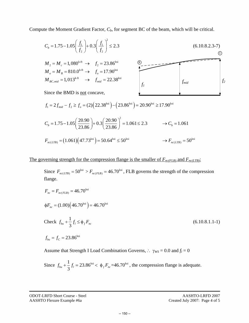
ODOT-LRFD Short Course - Steel AASHTO Flexure Example #6a
AASHTO-LRFD 2007 Created July 2007: Page 4 of 5
Compute the Moment Gradient Factor, Cb, for segment BC of the beam, which will be critical.
2
1 1
2 2
1.75 1.05 0.3 2.3bf fCf f
⎛ ⎞ ⎛ ⎞= − + ≤⎜ ⎟ ⎜ ⎟
⎝ ⎠ ⎝ ⎠ (6.10.8.2.3-7)
k-ft ksi2 2
k-ft ksi
k-ft ksi,
1,080 23.86
810.0 17.90
1,013 22.38
c
o B o
BC mid mid
M M f
M M f
M f
= = → =
= = → =
= → =
Since the BMD is not concave, ( ) ( )ksi ksi ksi ksi
1 22 (2) 22.38 23.86 20.90 17.90mid of f f f= − ≥ = − = ≥
220.90 20.901.75 1.05 0.3 1.061 2.3 1.061
23.86 23.86b bC C⎛ ⎞ ⎛ ⎞= − + = ≤ → =⎜ ⎟ ⎜ ⎟⎝ ⎠ ⎝ ⎠
( )( )ksi ksi ksi ksi
( ) ( )1.061 47.73 50.64 50 50nc LTB nc LTBF F= = ≤ → = The governing strength for the compression flange is the smaller of Fnc(FLB) and Fnc(LTB):
Since ksi ksi( ) ( )50 > 46.70nc LTB nc FLBF F= = , FLB governs the strength of the compression
flange.
ksi( ) 46.70nc nc FLBF F= =
( )ksi ksi(1.00) 46.70 46.70ncFφ = =
Check 13bu l f ncf f F+ ≤ φ (6.10.8.1.1-1)
ksi23.86bu Cf f= = Assume that Strength I Load Combination Governs, ∴ γWS = 0.0 and fl = 0
Since ksi ksi1 23.86 =46.703bu l f ncf f F+ = < φ , the compression flange is adequate.
B
C
f2fmidf1
-- 150 --

ODOT-LRFD Short Course - Steel AASHTO Flexure Example #6a
AASHTO-LRFD 2007 Created July 2007: Page 5 of 5
Investigate the Strength of the Tension Flange: Since the tension flange is discretely braced, ( )ksi ksi(1.0) 50 50nt h ytF R F= = = (6.10.8.3-1) ( )ksi ksi(1.00) 50 50ntFφ = =
Check 13bu l f ntf f F+ ≤ φ (6.10.8.1.2-1)
ksi23.86bu Cf f= =
Since ksi ksi1 23.86 =50.003bu l f ntf f F+ = < φ , the tension flange is adequate.
Since both the compression flange and tension flange are adequate, the section is adequate for flexure.
-- 151 --

ODOT-LRFD Short Course - Steel AASHTO Flexure Example #6b
AASHTO-LRFD 2007 Created July 2007: Page 1 of 7
AASHTO Flexural Example #6b: Problem: A non-composite built-up girder made of M270-50 steel is used to span 48’. The beam is braced laterally at 12’-0” intervals and is subjected to a factored load of w = 3.75kip/ft, which includes the self weight of the beam. Check to see if the section is adequate considering flexural failure modes at the Strength Limit States. If appropriate, use the provisions in AASHTO Appendix A6 to determine capacity. Solution:
Determine Classification of the Section:
Check ?2 5.7c
w yc
D Et F
≤ (6.10.6.2.3-1)
Take D = 38”
38" 19"2 2cDD = = =
ksi?
ksi38
(2)(19") 29,000101.3 5.7 137.3( ") 50
= ≤ = OK, ∴ web is non-slender
Check ?
0.3yc
yt
II
≥ (6.10.6.2.3-2)
Since Section is doubly symmetric, Iyc = Iyt OK
-- 152 --

ODOT-LRFD Short Course - Steel AASHTO Flexure Example #6b
AASHTO-LRFD 2007 Created July 2007: Page 2 of 7
Since the web is non-slender and Eq 6.10.6.2.3-2 is satisfied, we have the option of using either AASHTO Section 6.10.8 or Appendix A6 to determine the flexural capacity of this member. For this example, the provisions of A6 will be used and we will work with moments. The following failure modes must be investigated:
• Flange Local Buckling of the Compression Flange Mnc(FLB) • Lateral-Torsional Buckling Mnc(LTB) • Yielding of Tension Flange Mnt
Compute Web Plasticity Factors, Rpc and Rpt (Section A6.2): Investigate the classification of the web.
Check ?
( )
2cp
cppw D
w
Dt
≤λ (A6.2.1-1)
( ) 20.54
0.09cp
yc cppw D rw
cp
h y
EF D
DMR M
⎛ ⎞λ = ≤ λ ⎜ ⎟
⎛ ⎞ ⎝ ⎠−⎜ ⎟⎜ ⎟
⎝ ⎠
(A6.2.1-2)
5.7 137.3rwyc
EF
λ = = (A6.2.1-3)
Rh = 1.00 (since the section is rolled and is ∴ non-hybrid)
( )( )( )( )
3 ksi k-in k-ft
3 ksi k-in k-ft
543.1 in 50 27,160 2,263
600.4 in 50 30,020 2,502
y x y
p x y
M S F
M Z F
= = = =
= = = =
( )( )( )( )
ksi
ksi
( ) 2k-in
k-in
29,00019"50 93.68 137.3 137.319"0.54 30,020
0.091.0 27,160
cppw D⎛ ⎞λ = = ≤ =⎜ ⎟⎝ ⎠⎛ ⎞
⎜ ⎟−⎜ ⎟⎝ ⎠
( ) 93.68
cppw Dλ =
Mnc
-- 153 --

ODOT-LRFD Short Course - Steel AASHTO Flexure Example #6b
AASHTO-LRFD 2007 Created July 2007: Page 3 of 7
?
( )38
2 (2)(19") 101.3 93.68" cp
cppw D
w
Dt
= = >λ = ∴ web is non compact
Since the web is non compact,
( )
( )
1 1 c
c
w pw Dh yc p ppc
p rw pw D yc yc
R M M MR
M M M
⎡ ⎤⎛ ⎞⎛ ⎞ λ −λ= − − ≤⎢ ⎥⎜ ⎟⎜ ⎟⎜ ⎟⎜ ⎟λ −λ⎢ ⎥⎝ ⎠⎝ ⎠⎣ ⎦
(A6.2.2-4)
Where,
( ) ( )c cp
cppw D pw D rw
c
DD
⎛ ⎞λ = λ ≤ λ⎜ ⎟
⎝ ⎠ (A6.2.2-6)
19 ''93.68 137.319 ''
93.68 137.3
⎛ ⎞= ≤⎜ ⎟⎝ ⎠
= ≤
k-in k-in k-in
k-in k-in k-in
(1.00)(27,160 ) 101.3 93.68 (30,020 ) (30,020 )1 1(30,020 ) 137.3 93.68 (27,160 ) (27,160 )pcR
⎡ ⎤⎛ ⎞ −⎛ ⎞= − − ≤⎢ ⎥⎜ ⎟⎜ ⎟−⎝ ⎠⎝ ⎠⎣ ⎦
1.087 1.1051.087
= ≤=
( )
( )
1 1 c
c
w pw Dh yt p ppt
p rw pw D yt yt
R M M MR
M M M
⎡ ⎤⎛ ⎞⎛ ⎞ λ −λ= − − ≤⎢ ⎥⎜ ⎟⎜ ⎟⎜ ⎟⎜ ⎟λ −λ⎢ ⎥⎝ ⎠⎝ ⎠⎣ ⎦
(A6.2.2-5)
k-in k-in k-in
k-in k-in k-in
(1.00)(27,160 ) 101.3 93.68 (30,020 ) (30,020 )1 1(30,020 ) 137.3 93.68 (27,160 ) (27,160 )ptR
⎡ ⎤⎛ ⎞ −⎛ ⎞= − − ≤⎢ ⎥⎜ ⎟⎜ ⎟−⎝ ⎠⎝ ⎠⎣ ⎦
1.087 1.1051.087
= ≤=
Investigate Compression Flange Local Buckling: Investigate the compactness of the compression flange.
3
4
16" 10.672 (2)( ")
fcf
fc
bt
λ = = = (A6.3.2-3)
ksi
ksi
29,0000.38 0.38 9.15250pf
yc
EF
λ = = = (A6.3.2-4)
-- 154 --
ODOT-LRFD Short Course - Steel AASHTO Flexure Example #6b
AASHTO-LRFD 2007 Created July 2007: Page 4 of 7
Since λf >λpf, the flange is non compact and,
( ) 1 1 yr xc f pfnc FLB pc yc
pc yc rf pf
F SM R M
R M
⎡ ⎤⎛ ⎞⎛ ⎞λ −λ= − −⎢ ⎥⎜ ⎟⎜ ⎟⎜ ⎟⎜ ⎟λ −λ⎢ ⎥⎝ ⎠⎝ ⎠⎣ ⎦
(A6.3.2-2)
min 0.7 , , 0.5xtyr yc h yt yw yc
xc
SF F R F F FS
⎛ ⎞= ≥⎜ ⎟
⎝ ⎠ ; ( )ksi ksi(0.7) 50 35yrF = = (Pg 6-222)
0.95 crf
yr
EkF
λ = (A.6.3.2-5)
''
''38
4 4 0.397438
c
w
kDt
= = = (A6.3.2-6)
( )( )
( )ksi
ksi
29,000 0.39740.95 17.24
35rf = =λ
( )( )( )( ) ( )( )
ksi 3k-in
( ) k-in
35 543.1 in 10.67 9.1521 1 1.087 27,16017.24 9.1521.087 27,160nc FLBM
⎡ ⎤⎛ ⎞ −⎛ ⎞⎢ ⎥⎜ ⎟= − − ⎜ ⎟⎜ ⎟ −⎢ ⎥⎝ ⎠⎝ ⎠⎣ ⎦
k-in k-ft27,550 2,296= = Investigate Compression Flange Lateral-Torsional Buckling: The unbraced length of the beam is Lb = 12’-0” = 144.0”.
3
83
4
(16") 4.220"1 (19")( ")1 12 112 1 3 (16")( ")3
fct
c w
fc fc
br
D tb t
= = =⎛ ⎞ ⎛ ⎞⎛ ⎞++ ⎜ ⎟⎜ ⎟ ⎜ ⎟⎜ ⎟ ⎝ ⎠⎝ ⎠⎝ ⎠
(A6.3.3-10)
ksi
ksi
29,0001.0 (1.0)(4.220") 101.6"50p t
yc
EL rF
= = = (A6.3.3-4)
2
1.95 1 1 6.76 yr xcr t
yr xc
F S hE JL rF S h E J
⎛ ⎞= + + ⎜ ⎟
⎝ ⎠ (6.10.8.2.3-5)
min 0.7 , , 0.5xtyr yc h yt yw yc
xc
SF F R F F FS
⎛ ⎞= ≥⎜ ⎟
⎝ ⎠ ( )( )ksi ksi0.7 50 35yrF = = (Pg 6-222)
-- 155 --
ODOT-LRFD Short Course - Steel AASHTO Flexure Example #6b
AASHTO-LRFD 2007 Created July 2007: Page 5 of 7
( )( ) 312 438" " 38.75"fc fth D t t= + + = + =
3 33 1 0.63 1 0.63
3 3 3fc fc fc ft ft ftw
fc ft
b t t b t tD tJb b
⎛ ⎞ ⎛ ⎞= + − + −⎜ ⎟ ⎜ ⎟⎜ ⎟ ⎜ ⎟
⎝ ⎠ ⎝ ⎠ (A6.3.3-9)
( )3 33 3 3
48 4 4(38")( ") (16")( ") "(2) 1 0.63 5.035 in3 3 16"
J⎡ ⎤⎛ ⎞⎛ ⎞= + − =⎢ ⎥⎜ ⎟⎜ ⎟⎝ ⎠⎝ ⎠⎣ ⎦
ksi
ksi
29,000 828.635yr
EF
= =
( )( )3
4
543.1 in 38.75"4,180
5.035 inxcS hJ
= =
( )( )( )21 4,1801.95 4.220" 828.6 1 1 6.76 396.8" 33.06 '
4,180 828.6rL ⎛ ⎞= + + = =⎜ ⎟⎝ ⎠
Since 101.6" 144" 396.8"p b rL L L= < = < = , Inelastic LTB must be investigated.
( ) 1 1 yr xc b pnc LTB b pc yc pc yc
pc yc r p
F S L LM C R M R M
R M L L
⎡ ⎤⎛ ⎞⎛ ⎞−= − − ≤⎢ ⎥⎜ ⎟⎜ ⎟⎜ ⎟⎜ ⎟−⎢ ⎥⎝ ⎠⎝ ⎠⎣ ⎦
(A6.3.3-2)
( )( )( )( ) ( )( ) ( )( )
( )( )( ) ( )( )
ksi 3k-in k-in
( ) k-in
k-in k-in k-in
35 543.1 in 144" 101.6"1 1 1.087 27,160 1.087 27,160396.8" 101.6"1.087 27,160
0.9488 29,520 28,010 29,520
nc LTB b
b b
M C
C C
⎡ ⎤⎛ ⎞ −⎛ ⎞⎢ ⎥⎜ ⎟= − − ≤⎜ ⎟⎜ ⎟ −⎢ ⎥⎝ ⎠⎝ ⎠⎣ ⎦
= = ≤
-- 156 --

ODOT-LRFD Short Course - Steel AASHTO Flexure Example #6b
AASHTO-LRFD 2007 Created July 2007: Page 6 of 7
Compute the Moment Gradient Factor, Cb, for segment BC of the beam, which will be critical.
2
1 1
2 2
1.75 1.05 0.3 2.3bM MCM M
⎛ ⎞ ⎛ ⎞= − + ≤⎜ ⎟ ⎜ ⎟
⎝ ⎠ ⎝ ⎠ (A6.3.3-7)
k-ft2
k-ft
k-ft,
1,080
810.0
1,013
c
o B
BC mid
M M
M M
M
= =
= =
=
Since the BMD is not concave, ( ) ( )k-ft k-ft k-ft k-ft
1 22 (2) 1,013 1,080 946 810mid oM M M M= − ≥ = − = ≥
2946 9461.75 1.05 0.3 1.061 2.31,080 1,080
1.061
bC ⎛ ⎞ ⎛ ⎞= − + = ≤⎜ ⎟ ⎜ ⎟⎝ ⎠ ⎝ ⎠
=
( )( )k-in k-in k-in
( ) 1.061 28,010 29,720 29,520nc LTBM = = ≤ k-in k-ft
( ) 29,520 2,460nc LTBM = = The governing strength for the compression flange is the smaller of Mnc(FLB) and Mnc(LTB):
Since k-ft k-ft( ) ( )2, 460 > 2, 296nc LTB nc FLBM M= = , ∴ FLB governs the strength of the
compression flange.
k-ft( ) 2, 296nc nc FLBM M= =
( )k-ft k-ft(1.00) 2,296 2,296ncMφ = =
Check 13u l xc f ncM f S M+ ≤ φ (A6.1.1-1)
k-ft1,080u CM M= = Assume that Strength I Load Combination Governs, ∴ γWS = 0.0 and fl = 0
Since k-ft k-ft1 1,080 =2,2963u l xc f ncM f S M+ = < φ , the compression flange is adequate.
-- 157 --

ODOT-LRFD Short Course - Steel AASHTO Flexure Example #6b
AASHTO-LRFD 2007 Created July 2007: Page 7 of 7
Investigate the Strength of the Tension Flange: Since the tension flange is discretely braced, ( )k-in k-in k-ft(1.087) 27,160 29,520 2,460nt pt ytM R M= = = = (A6.4-1) ( )k-ft k-ft(1.00) 2,460 2,460ntMφ = =
Check 13u l xt f ntM f S M+ ≤ φ (6.10.8.1.2-1)
k-ft1,080u CM M= =
Since k-ft k-ft1 1,080 =2,4603u l xt f ntM f S M+ = < φ , the tension flange is adequate.
Since both flanges are adequate, the section is adequate for flexure.
Note that the benefits of using Appendix A6 are illustrated here. Even though the capacity was found to be adequate in both Examples #6a and #6b, using Appendix A6, the capacity was found to be 16% greater than the capacity found using the provisions in Section 6.10.8.
-- 158 --
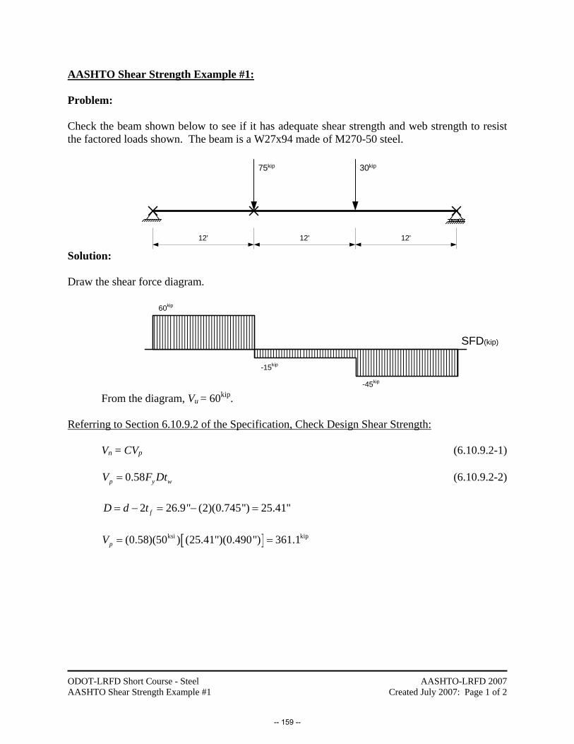
ODOT-LRFD Short Course - Steel AASHTO Shear Strength Example #1
AASHTO-LRFD 2007 Created July 2007: Page 1 of 2
AASHTO Shear Strength Example #1: Problem: Check the beam shown below to see if it has adequate shear strength and web strength to resist the factored loads shown. The beam is a W27x94 made of M270-50 steel.
Solution: Draw the shear force diagram.
From the diagram, Vu = 60kip.
Referring to Section 6.10.9.2 of the Specification, Check Design Shear Strength:
Vn = CVp (6.10.9.2-1)
0.58p y wV F Dt= (6.10.9.2-2)
2 26.9" (2)(0.745") 25.41"fD d t= − = − =
[ ]ksi kip(0.58)(50 ) (25.41")(0.490") 361.1pV = =
75kip
12' 12'12'
30kip
SFD(kip)
60kip
-15kip
-45kip
-- 159 --
ODOT-LRFD Short Course - Steel AASHTO Shear Strength Example #1
AASHTO-LRFD 2007 Created July 2007: Page 2 of 2
Since the web is unstiffened, k = 5.00.
( )( )( )
ksi
ksi
29,000 5.0053.85
50y
EkF
= =
( )( )1.12 1.12 53.85 60.31y
EkF
= = 25.41" 51.860.490"w
Dt= =
Since 51.86 1.12 60.31w y
D Ekt F
= < = , shear yielding governs and,
C = 1.00 (6.10.9.3.2-4) Vn = CVp = (1.00)(361.1kip) = 361.1kip φVn = (1.00)(361.1kip) = 361.1kip > Vu = 60kip O.K.
-- 160 --

ODOT-LRFD Short Course - Steel AASHTO Shear Strength Example #2
AASHTO-LRFD 2007 Created July 2007: Page 1 of 3
AASHTO Shear Strength Example #2: Problem: A built-up section made of M270-50 steel, is used as a beam. Determine the design shear capacity of the beam and determine if the beam can sustain a factored shear force of 242kip. Solution: Referring to Section 6.10.9.2 of the Specification:
Vn = CVp (6.10.9.2-1)
0.58p y wV F Dt= (6.10.9.2-2)
[ ]ksi kip38(0.58)(50 ) (38")( ") 413.3pV = =
Since the web is unstiffened, k = 5.00.
( )( )( )
ksi
ksi
29,000 5.0053.85
50y
EkF
= =
( )( )1.12 1.12 53.85 60.31y
EkF
= =
( )( )1.40 1.40 53.85 75.39y
EkF
= = 3
8
38" 101.3"w
Dt= =
Since 101.3 1.40 75.39w y
D Ekt F
= > = , Elastic shear buckling governs and,
( )( )( )
( )( )( )
ksi
2 2 ksi
29,000 5.001.571.57 0.443750/ 101.3yw
EkCFD t
⎛ ⎞⎛ ⎞⎜ ⎟= = =⎜ ⎟⎜ ⎟ ⎜ ⎟⎝ ⎠ ⎝ ⎠
(6.10.9.3.2-6)
Vn = CVp = (0.4437) (413.3kip) = 183.4kip φVn = (1.00)(183.4kip) = 183.4kip < Vu = 242kip
-- 161 --
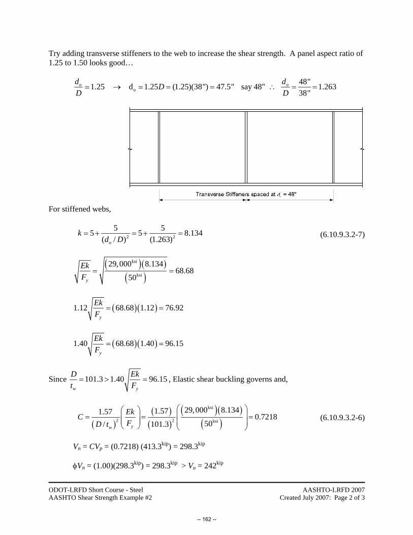
ODOT-LRFD Short Course - Steel AASHTO Shear Strength Example #2
AASHTO-LRFD 2007 Created July 2007: Page 2 of 3
Try adding transverse stiffeners to the web to increase the shear strength. A panel aspect ratio of 1.25 to 1.50 looks good…
o48"1.25 d 1.25 (1.25)(38") 47.5" say 48" 1.26338"
o od dDD D
→ = = ∴ = =
For stiffened webs,
2 2
5 55 5 8.134( / ) (1.263)o
kd D
= + = + = (6.10.9.3.2-7)
( )( )( )
ksi
ksi
29,000 8.13468.68
50y
EkF
= =
( )( )1.12 68.68 1.12 76.92y
EkF
= =
( )( )1.40 68.68 1.40 96.15y
EkF
= =
Since 101.3 1.40 96.15w y
D Ekt F
= > = , Elastic shear buckling governs and,
( )( )( )
( )( )( )
ksi
2 2 ksi
29,000 8.1341.571.57 0.721850/ 101.3yw
EkCFD t
⎛ ⎞⎛ ⎞⎜ ⎟= = =⎜ ⎟⎜ ⎟ ⎜ ⎟⎝ ⎠ ⎝ ⎠
(6.10.9.3.2-6)
Vn = CVp = (0.7218) (413.3kip) = 298.3kip φVn = (1.00)(298.3kip) = 298.3kip > Vu = 242kip
-- 162 --

ODOT-LRFD Short Course - Steel AASHTO Shear Strength Example #2
AASHTO-LRFD 2007 Created July 2007: Page 3 of 3
The previous calculations were based on the buckling strength of the web. For interior panels where:
( )2 2.5w
fc fc ft ft
Dtb t b t
≤+
(6.10.9.3.2-1)
[ ]3
8
3 34 4
(2)(38")( ") 28.5 1.188 2.5(16")( ") (16")( ") 24.0
= = ≤+
OK
Tension Field Action can be developed:
2
0.87(1 )
1n p
o
CV V CdD
⎡ ⎤⎢ ⎥
−⎢ ⎥= +⎢ ⎥⎛ ⎞⎢ ⎥+ ⎜ ⎟⎢ ⎥⎝ ⎠⎣ ⎦
(6.10.9.3.2-2)
( )kip kip
2
(0.87)(1 0.7218)(413.3 ) (0.7218) 360.41 1.263
nV⎡ ⎤
−⎢ ⎥= + =⎢ ⎥+⎣ ⎦
φVn = (1.00)(360.4kip) = 360.4kip
-- 163 --

-- 164 --

ODOT-LRFD Short Course - Steel AASHTO Web Strength Example #1
AASHTO-LRFD 2007 Created July 2007: Page 1 of 3
AASHTO Web Strength Example #1: Problem: Check the beam shown below to see if it has adequate shear strength and web strength to resist the factored loads shown. The beam is a W27x94 made of M270-50 steel.
Solution: Draw the shear force diagram.
Referring to Section D6.5 of the Specification, Check the End Reactions for Web Yielding and Web Crippling: (Assume that the bearing length, N, is 3-1/4”.) Check Web Yielding
Since the supports are likely to be at a distance less than or equal to d from the end of the member:
(2.5 )n yw wR k N F t= + (D6.5.2-3)
ksi kip((2.5)(1.34") 3.25")(50 )(0.490") 161.7nR = + =
kip kip(1.0)(161.7 ) 161.7nRφ = = > 60kip O.K.
SFD(kip)
60kip
-15kip
-45kip
75kip
12' 12'12'
30kip
-- 165 --
ODOT-LRFD Short Course - Steel AASHTO Web Strength Example #1
AASHTO-LRFD 2007 Created July 2007: Page 2 of 3
Check Web Crippling
Since the supports are likely to be at a distance less than or equal to d/2 from the end of the member.
Check Nd
:
3.25" 0.1208 0.2026.9"
= ≤
Therefore, (D6.5.3-3) controls: 1.5
20.40 1 3 yw fwn w
f w
EF ttNR td t t
⎡ ⎤⎛ ⎞⎛ ⎞⎢ ⎥= + ⎜ ⎟⎜ ⎟⎜ ⎟⎢ ⎥⎝ ⎠⎝ ⎠⎣ ⎦
1.5 ksi ksi
2 3.25" 0.490" (29,000 )(50 )(0.745")0.40(0.490") 1 326.9" 0.745" 0.490"nR
⎡ ⎤⎛ ⎞⎛ ⎞= +⎢ ⎥⎜ ⎟⎜ ⎟⎝ ⎠⎝ ⎠⎢ ⎥⎣ ⎦
2 ksi kip(0.09604 in )(1.193)(1485 ) 170.2nR = =
kip kip(0.80)(170.2 ) 136.2nRφ = = > 60kip O.K.
Check the Interior Concentrated Loads for Web Yielding and Web Crippling: (Assume that the bearing length, N, is 3.25”) Check Web Yielding
Since the applied load is located at a distance greater than d from the end of the member.
(5 )n yw wR k N F t= + (D6.5.2-2)
ksi kip((5)(1.34") 3.25")(50 )(0.490") 243.8nR = + =
kip kip(1.0)(243.8 ) 243.8nRφ = = > 75kip O.K.
-- 166 --
ODOT-LRFD Short Course - Steel AASHTO Web Strength Example #1
AASHTO-LRFD 2007 Created July 2007: Page 3 of 3
Check Web Crippling
Since the applied load is located at a distance greater than d/2 from the end of the member.
Therefore, (D6.5.3-2) controls: 1.5
20.80 1 3 yw fwn w
f w
EF ttNR td t t
⎡ ⎤⎛ ⎞⎛ ⎞⎢ ⎥= + ⎜ ⎟⎜ ⎟⎜ ⎟⎢ ⎥⎝ ⎠⎝ ⎠⎣ ⎦
1.5 ksi ksi
2 3.25" 0.490" (29,000 )(50 )(0.745")0.80(0.490") 1 326.9" 0.745" 0.490"nR
⎡ ⎤⎛ ⎞⎛ ⎞= +⎢ ⎥⎜ ⎟⎜ ⎟⎝ ⎠⎝ ⎠⎢ ⎥⎣ ⎦
2 ksi kip(0.1921 in )(1.193)(1485 ) 340.3nR = =
kip kip(0.80)(340.3 ) 272.2nRφ = = > 75kip O.K.
The Web Yielding and Web Crippling Strengths are Satisfactory
-- 167 --

ODOT-LRFD Short Course - Steel AASHTO Web Strength Example #2
AASHTO-LRFD 2007 Created July 2007: Page 1 of 6
AASHTO Web Strength Example #2: Problem: A built-up section made of M270-50 steel, is used as a beam. It was determined in AASHTO Shear Strength Example #2 that intermediate stiffeners were required to develop adequate shear strength in the web. Determine the required size of these intermediate stiffeners. And check the web to see if an end reaction of 128kip can be supported. Solution:
Design the intermediate stiffeners that were added to increase the shear strength: The moment of inertia of the intermediate stiffeners should satisfy the smaller of: 3
t wI bt J≥ (6.10.11.1.3-1) and
1.54 1.3
40ywt
t
FDIE
ρ ⎛ ⎞≥ ⎜ ⎟
⎝ ⎠ (6.10.11.1.3-2)
where: It - Moment of inertia of the stiffener pair about the mid-thickness of the web.
2
2.5 2.0 0.5/o
DJd D
⎛ ⎞= − ≥⎜ ⎟
⎝ ⎠ use…
( )22.5 2.0 0.5/o
Jd D
= − ≥ (6.10.11.1.3-3)
-- 168 --
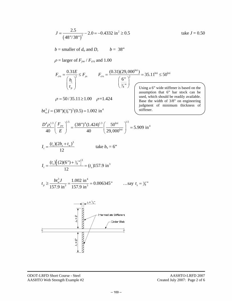
ODOT-LRFD Short Course - Steel AASHTO Web Strength Example #2
AASHTO-LRFD 2007 Created July 2007: Page 2 of 6
( )
22
2.5 2.0 0.4332 in 0.548"/ 38"
J = − = − ≥ take J = 0.50
b = smaller of do and D, b = 38” ρ = larger of Fyw / Fcrs and 1.00
ksi
ksi ksi2 2
38
0.31 (0.31)(29,000 ) 35.11 50 6"
"
crs ys crs
t
p
EF F Fbt
= ≤ = = ≤⎛ ⎞ ⎛ ⎞⎜ ⎟ ⎜ ⎟⎜ ⎟ ⎝ ⎠⎝ ⎠
50 / 35.11 1.00 =1.424ρ ρ= ≥ 3 3 43
8(38")( ") (0.5) 1.002 inwbt j = =
1.5 1.54 1.3 4 1.3 ksi
4ksi
(38") (1.424) 50 5.909 in40 40 29,000
ywt FDE
⎛ ⎞ ⎛ ⎞= =⎜ ⎟ ⎜ ⎟
⎝ ⎠⎝ ⎠
ρ
3( )(2 )
12s s w
tt b tI +
= take bs = 6”
[ ]338 3( ) (2)(6") "
( )157.9 in12
st s
tI t
+= =
3 4
3 3
1.002 in 0.006345"157.9 in 157.9 in
wp
bt Jt ≥ = = …say 38 "st =
Using a 6” wide stiffener is based on the assumption that 6” bar stock can be used, which should be readily available. Base the width of 3/8” on engineering judgment of minimum thickness of stiffener.
-- 169 --

ODOT-LRFD Short Course - Steel AASHTO Web Strength Example #2
AASHTO-LRFD 2007 Created July 2007: Page 3 of 6
Referring to SectionD6.5 of the Manual, Check the End Reactions for Web Yielding and Web Crippling: The bearing length, N, is 9” and we’ll assume that 3/8” fillet welds connect the flanges and web. This gives an effective “k” distance of 3/4” + 3/8” = 1.125” Check Web Yielding
Since the supports are likely to be at a distance less than or equal to d from the end of the member.
(2.5 )n yw wR k N F t= + (D6.5.2-3)
ksi kip38((2.5)(1.125") 9")(50 )( ") 221.5nR = + =
kip kip(1.0)(221.5 ) 221.5nRφ = = > 128kip O.K.
Check Web Crippling
Since the supports are likely to be at a distance less than or equal to d/2 from the end of the member.
Check Nd
:
34
9" 0.2278 0.2038" (2)( ")
= >+
Therefore, (D6.5.3-4) controls: 1.5
2 40.40 1 0.2 yw fwn w
f w
EF ttNR td t t
⎡ ⎤⎛ ⎞⎛ ⎞⎢ ⎥= + − ⎜ ⎟⎜ ⎟⎜ ⎟⎢ ⎥⎝ ⎠⎝ ⎠⎣ ⎦
1.5 ksi ksi3 3
2 8 438 3 3 3
4 4 8
(4)(9") " (29,000 )(50 )( ")(0.40)( ") 1 0.2(38" (2)( ") " ( ")nR
⎡ ⎤⎛ ⎞⎛ ⎞= + −⎢ ⎥⎜ ⎟⎜ ⎟+ ⎝ ⎠⎝ ⎠⎢ ⎥⎣ ⎦
2 ksi kip(0.05625 in )(1.252)(1,703 ) 119.9nR = =
kip kip(0.80)(119.9 ) 95.92nRφ = = <128kip No Good.
The web strength is satisfactory with regard to web yielding but not for web crippling. Bearing stiffeners will need to be added. (Technically speaking, stiffeners are required by AASHTO at all bearing locations on built-up sections anyways…)
-- 170 --
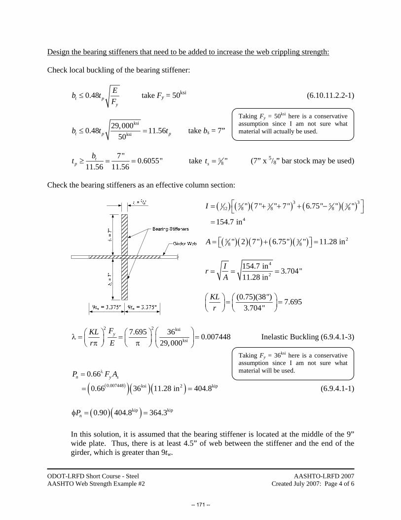
ODOT-LRFD Short Course - Steel AASHTO Web Strength Example #2
AASHTO-LRFD 2007 Created July 2007: Page 4 of 6
Design the bearing stiffeners that need to be added to increase the web crippling strength: Check local buckling of the bearing stiffener:
0.48t py
Eb tF
≤ take Fy = 50ksi (6.10.11.2.2-1)
ksi
ksi
29,0000.48 11.5650t p pb t t≤ = take bs = 7”
7" 0.6055"11.56 11.56
tp
bt ≥ = = take 58 "st = (7” x 5/8” bar stock may be used)
Check the bearing stiffeners as an effective column section:
( ) ( )( ) ( )( )3 35 3 5 3112 8 8 8 8
4
" 7" " 7" 6.75" " "
154.7 in
I ⎡ ⎤= + + + −⎣ ⎦=
( )( )( ) ( )( ) 25 3
8 8" 2 7" 6.75" " 11.28 inA = + =⎡ ⎤⎣ ⎦
4
2
154.7 in 3.704"11.28 in
IrA
= = =
(0.75)(38") 7.695
3.704"KLr
⎛ ⎞ ⎛ ⎞= =⎜ ⎟ ⎜ ⎟⎝ ⎠ ⎝ ⎠
2 2 ksi
ksi
7.695 36 0.00744829,000
yFKLr E
⎛ ⎞⎛ ⎞ ⎛ ⎞λ = = =⎜ ⎟⎜ ⎟ ⎜ ⎟π π⎝ ⎠ ⎝ ⎠ ⎝ ⎠ Inelastic Buckling (6.9.4.1-3)
0.66n y sP F Aλ=
( )( ) ( )( )0.007448 ksi 2 kip0.66 36 11.28 in 404.8= = (6.9.4.1-1)
( )( )kip kip0.90 404.8 364.3nPφ = =
In this solution, it is assumed that the bearing stiffener is located at the middle of the 9” wide plate. Thus, there is at least 4.5” of web between the stiffener and the end of the girder, which is greater than 9tw.
Taking Fy = 50ksi here is a conservative assumption since I am not sure what material will actually be used.
Taking Fy = 36ksi here is a conservative assumption since I am not sure what material will be used.
-- 171 --
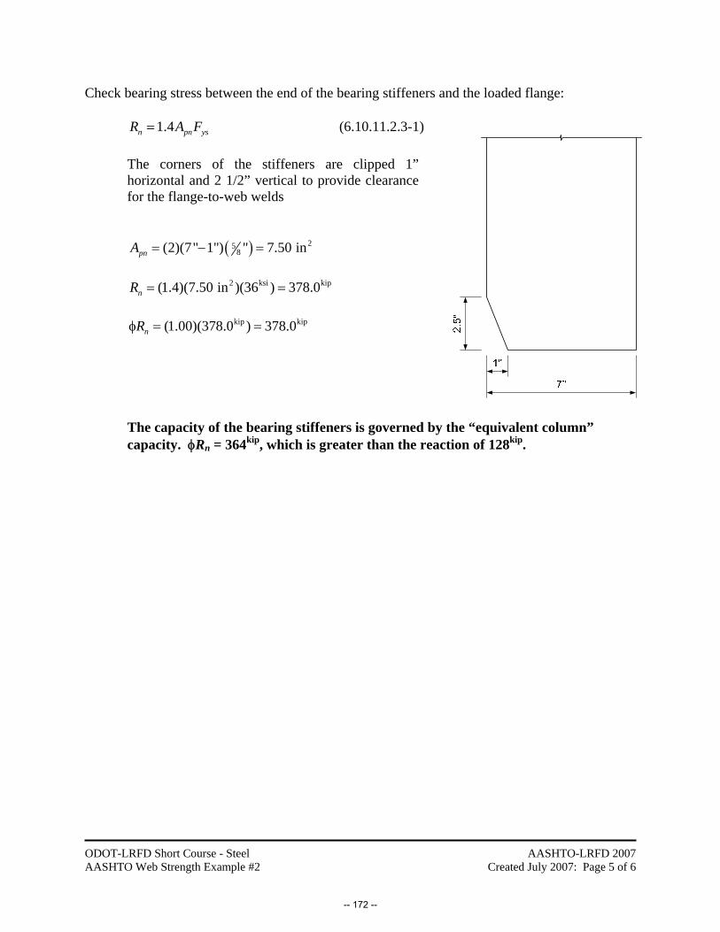
ODOT-LRFD Short Course - Steel AASHTO Web Strength Example #2
AASHTO-LRFD 2007 Created July 2007: Page 5 of 6
Check bearing stress between the end of the bearing stiffeners and the loaded flange: 1.4n pn ysR A F= (6.10.11.2.3-1)
The corners of the stiffeners are clipped 1” horizontal and 2 1/2” vertical to provide clearance for the flange-to-web welds
( ) 25
8(2)(7" 1") " 7.50 inpnA = − = 2 ksi kip(1.4)(7.50 in )(36 ) 378.0nR = = kip kip(1.00)(378.0 ) 378.0nRφ = =
The capacity of the bearing stiffeners is governed by the “equivalent column” capacity. φRn = 364kip, which is greater than the reaction of 128kip.
-- 172 --

ODOT-LRFD Short Course - Steel AASHTO Web Strength Example #2
AASHTO-LRFD 2007 Created July 2007: Page 6 of 6
Just for fun ☺, lets check the capacity of 2 pairs of 7” x 5/8” interior bearing stiffeners: The local buckling check will be the same as for the single pair of bearing stiffeners. Check the bearing stiffeners as an effective column section:
( ) ( )( ) ( )( )( )3 3 45 3 5 31
12 8 8 8 8(2) " 7" " 7" (2)(3.375") 7" (2) " " 309.5 inI ⎡ ⎤= + + + + − =⎣ ⎦
( )( )( ) ( ) ( ) 25 3
8 8" 4 7" (2) 3.375" 7" " 22.66 inA ⎡ ⎤= + + =⎡ ⎤⎣ ⎦⎣ ⎦
4
2
309.5 in 3.696"22.66 in
IrA
= = = (0.75)(38") 7.7113.696"
KLr
⎛ ⎞ ⎛ ⎞= =⎜ ⎟ ⎜ ⎟⎝ ⎠ ⎝ ⎠
2 2 ksi
ksi
7.711 36 0.00747929,000
yFKLr E
⎛ ⎞⎛ ⎞ ⎛ ⎞λ = = =⎜ ⎟⎜ ⎟ ⎜ ⎟π π⎝ ⎠ ⎝ ⎠ ⎝ ⎠ Inelastic Buckling (6.9.4.1-3)
( )( )( )( )0.007479 ksi 2 kip0.66 0.66 36 22.66 in 813.2n y sP F Aλ= = = (6.9.4.1-1)
( )( )kip kip0.90 813.2 731.9nPφ = = The bearing stress between the end of the bearing stiffeners and the loaded flange would be twice that calculated for a single pair of stiffeners: φRn = (2)(378.0kip) = 756.0kip. The strength is governed again by the “equivalent column” capacity, φRn = 732kip.
-- 173 --

-- 174 --
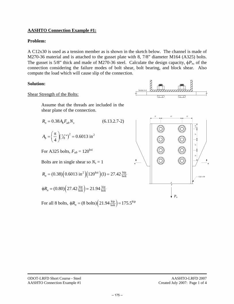
ODOT-LRFD Short Course - Steel AASHTO Connection Example #1
AASHTO-LRFD 2007 Created July 2007: Page 1 of 4
AASHTO Connection Example #1: Problem: A C12x30 is used as a tension member as is shown in the sketch below. The channel is made of M270-36 material and is attached to the gusset plate with 8, 7/8” diameter M164 (A325) bolts. The gusset is 5/8” thick and made of M270-36 steel. Calculate the design capacity, φPn, of the connection considering the failure modes of bolt shear, bolt bearing, and block shear. Also compute the load which will cause slip of the connection. Solution: Shear Strength of the Bolts:
Assume that the threads are included in the shear plane of the connection.
0.38n b ub sR A F N= (6.13.2.7-2)
( )2 278 " 0.6013 in
4bA π⎛ ⎞= =⎜ ⎟⎝ ⎠
For A325 bolts, Fub = 120ksi
Bolts are in single shear so Ns = 1
( )( ) kip2 ksibolt(0.38) 0.6013 in 120 (1) 27.42nR = =
( )kip kipbolt bolt(0.80) 27.42 21.94nRφ = =
For all 8 bolts, ( )kip kip
bolt(8 bolts) 21.94 175.5nRφ = =
A
3"
3"3"
1.5"
3" 6"
Pu
A
Section A-A
C12 x 30
3"
-- 175 --

ODOT-LRFD Short Course - Steel AASHTO Connection Example #1
AASHTO-LRFD 2007 Created July 2007: Page 2 of 4
Check Bearing Strength: Interior Bolts Bearing on the Channel Web: ( )( )( )71 1
2 8 163" 2 " " 2.063"cL = − + = Since Lc = 2.063” > 2d = 1.75”, 2.4n uR dtF= ( ) ( ) kipksi7
8 bolt(2.4) " (0.510") 58 62.11nR = = (6.13.2.9-1)
Interior Bolts Bearing on the Gusset Plate: ( )( )( )71 1
2 8 163" 2 " " 2.063"cL = − + = Since Lc = 2.063” > 2d = 1.75”, 2.4n uR dtF= ( )( )( ) kipksi7 5
8 8 bolt(2.4) " " 58 76.13nR = = (6.13.2.9-1)
End Bolts Bearing on the Channel Web: ( )( )71 1
2 8 161.5" " " 1.031"cL = − + = Since Lc = 1.031” < 2d = 1.75”, 1.2n c uR L tF= ( ) ( ) kipksi
bolt(1.2) 1.031" (0.510") 58 36.60nR = = (6.13.2.9-2)
End Bolts Bearing on the Gusset Plate: (Assume that the end distance on the gusset is 11/2”) ( )( )71 1
2 8 161.5" " " 1.031"cL = − + = Since Lc = 1.031” < 2d = 1.75”, 1.2n c uR L tF= ( )( )( ) kipksi5
8 bolt(1.2) 1.031" " 58 44.85nR = = (6.13.2.9-2)
For all 8 Bolts: ( ) ( ) ( )kip kip kip kip
bolt bolt bolt(2 bolts) 44.85 (4 bolts) 62.11 (2 bolts) 36.60 411.3nR = + + =
( )kip kip(0.80) 411.3 329.1nRφ = =
-- 176 --
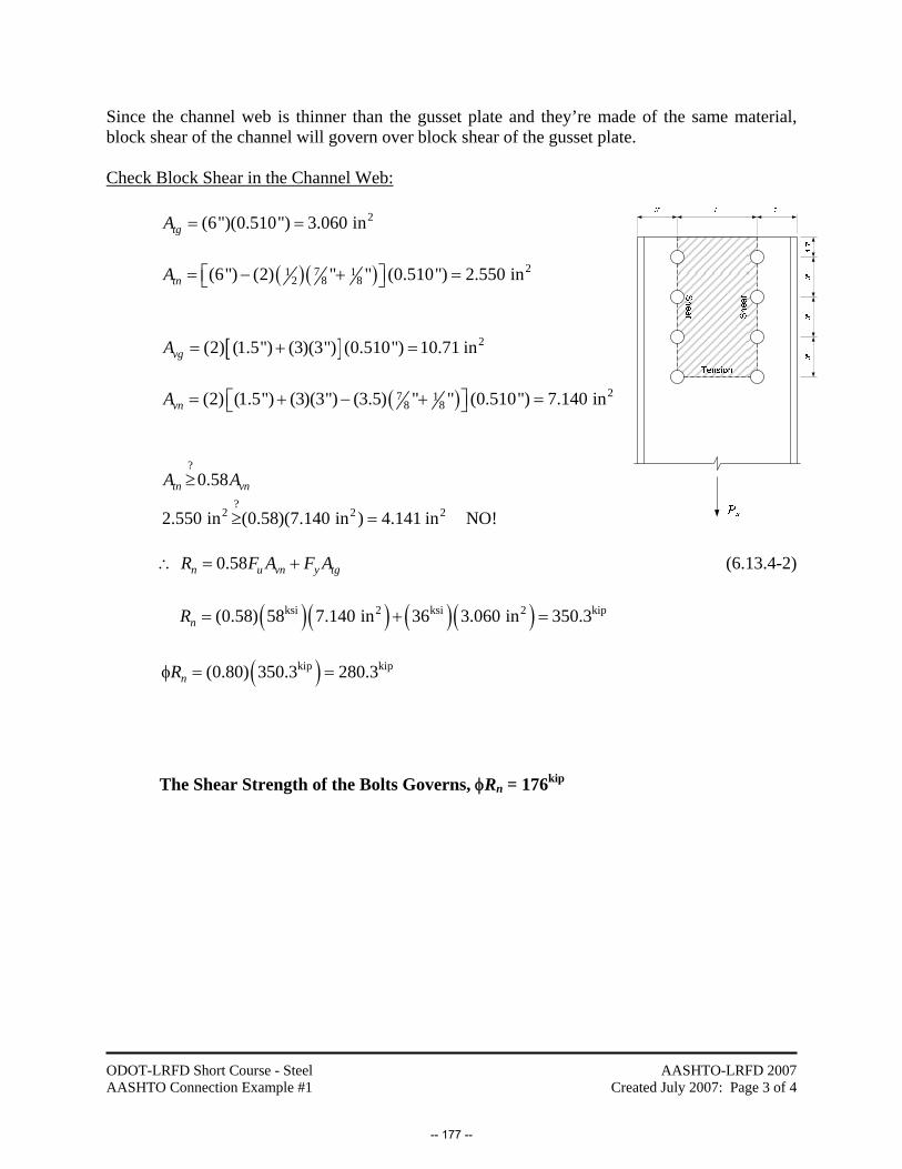
ODOT-LRFD Short Course - Steel AASHTO Connection Example #1
AASHTO-LRFD 2007 Created July 2007: Page 3 of 4
Since the channel web is thinner than the gusset plate and they’re made of the same material, block shear of the channel will govern over block shear of the gusset plate. Check Block Shear in the Channel Web: 2(6")(0.510") 3.060 intgA = = ( )( ) 271 1
2 8 8(6") (2) " " (0.510") 2.550 intnA = − + =⎡ ⎤⎣ ⎦ [ ] 2(2) (1.5") (3)(3") (0.510") 10.71 invgA = + = ( ) 27 1
8 8(2) (1.5") (3)(3") (3.5) " " (0.510") 7.140 invnA = + − + =⎡ ⎤⎣ ⎦
?
?2 2 2
0.58
2.550 in (0.58)(7.140 in ) 4.141 in NO!
tn vnA A≥
≥ =
0.58n u vn y tgR F A F A∴ = + (6.13.4-2) ( )( ) ( )( )ksi 2 ksi 2 kip (0.58) 58 7.140 in 36 3.060 in 350.3nR = + =
( )kip kip(0.80) 350.3 280.3nRφ = =
The Shear Strength of the Bolts Governs, φRn = 176kip
-- 177 --

ODOT-LRFD Short Course - Steel AASHTO Connection Example #1
AASHTO-LRFD 2007 Created July 2007: Page 4 of 4
Check the Slip Capacity of the Connection: n h s s tR K K N P= (6.13.2.8-1)
Kh = 1.00 (for standard holes) Ks = 0.33 (assume Class A surface) Ns = 1 Pt = 39kip (from Table 6.13.2.8-1 for M164 Bolts)
( ) kipkip
bolt(1.00)(0.33)(1) 39 12.87nR = =
For All 8 Bolts: ( )kip kip
bolt(8 bolts) 12.87 103.0nR = =
-- 178 --

ODOT-LRFD Short Course - Steel AASHTO Connection Example #2
AASHTO-LRFD 2007 Created July 2007: Page 1 of 2
AASHTO Connection Example #2: Problem: An 8” long WT 10.5 x 66 is attached to the bottom flange of a beam as is shown below. This hanger must support a factored load of 120kip. Given that 4, 1” diameter M164 (A325) bolts are used to attach the hanger to the beam, investigate the adequacy of the bolts and tee flange. Solution: Prying must be investigated in this situation:
33
8 20ub tQ Pa
⎛ ⎞= −⎜ ⎟⎝ ⎠
(6.13.2.10.4-1)
181
7" 1 " 2.375"2 2
tgb k= − = − = (k1 = 11/8” for W21 x 132)
( )( ) ( )( )1 1
2 2 12.4" 7" 2.700"f ta b g= − = − =
3(3)(2.375") (1.04") 0.2736
(8)(2.700") 20u u uQ P P⎛ ⎞
= − =⎜ ⎟⎝ ⎠
( )kip kip1.274 (1.274) 120 152.8u u u uT Q P P= + = = = Tensile Resistance of the Bolts: 0.76n b ubT A F= (6.13.2.10.2-1)
( )2 21" 0.7854 in4bA π⎛ ⎞= =⎜ ⎟
⎝ ⎠
Fub = 120ksi
( )( ) kip2 ksi
bolt(0.76) 0.7854 in 120 71.63nT = = ( )kip kipbolt bolt(0.80) 71.63 57.30nTφ = =
For All 4 Bolts: ( )kip kip
bolt(4 bolts) 57.30 229.2nTφ = = OK
-- 179 --

ODOT-LRFD Short Course - Steel AASHTO Connection Example #2
AASHTO-LRFD 2007 Created July 2007: Page 2 of 2
Check the Strength of the Flange of the WT: Assume that a plastic mechanism forms between the bolt lines and stem. Moment Equilibrium about at the fillet:
22u
uP bM M ⎛ ⎞→ = ⎜ ⎟
⎝ ⎠∑
( )kip
k-in
120 (2.375")4
71.25
uM⎛ ⎞⎜ ⎟=⎜ ⎟⎝ ⎠
=
For Safety, p uM Mφ ≥ . ( )2
ksi k-in(8")(1.04") 50 108.24 4p y
LtM F ⎛ ⎞= = =⎜ ⎟⎝ ⎠
( )k-in k-in(1.00) 108.2 108.2pMφ = = OK
Mu
Pu/2
Mu
Tu
QQ T T
Pu
b
-- 180 --

ODOT-LRFD Short Course - Steel AASHTO Connection Example #3
AASHTO-LRFD 2007 Created July 2007: Page 1 of 1
AASHTO Connection Example #3: Problem: Assuming an unfactored fatigue load of 60kip, determine the fatigue life of the tension bolts in the previous example. Solution: For Safety, ( ) ( )n
f Fγ Δ ≤ Δ (6.6.1.2.2-1)
( ) ( ) ( )( )( )
kipksi
2
(0.75) 1.274 6018.24
(4) 0.7854 inbolts
Pf
A
⎡ ⎤γ Δ ⎣ ⎦γ Δ = = =
( ) ( )13
2TH
n
FAFN
Δ⎛ ⎞Δ = ≥⎜ ⎟⎝ ⎠
For infinite life, ( ) ( ) ksiksi31.0 15.5
2 2TH
n
FF
ΔΔ = = =
Since ( ) ( )ksi ksi18.24 15.5
nf Fγ Δ = > Δ = , the bolts will have a finite life
For finite life, ( ) ( )13
n
Af FN
⎛ ⎞γ Δ ≤ Δ = ⎜ ⎟⎝ ⎠
( )( ) ( )
8 3
3 3ksi
17.1 10 ksi 281,800 cycles18.24
ANf
×≤ = =
γ Δ
Note that if prying is not included, ( ) ksi14.32fγ Δ = and the calculations would incorrectly show that the bolts have an infinite fatigue life.
-- 181 --

ODOT-LRFD Short Course - Steel AASHTO Connection Example #4
AASHTO-LRFD 2007 Created July 2007: Page 1 of 3
AASHTO Connection Example #4: Problem: Suppose that the hanger depicted in Examples #2 and #3 is subjected to a force that is applied at an angle as is shown below. Determine if the connection is adequate in this configuration. Solution:
kip2 0.8944 107.35u
u uPV P= = =
kip
kipbolt
107.3 26.834 boltsuV = =
kip1.274 0.5694 68.335
uu u
PT P= = =
kip
kipbolt
68.33 17.084 boltsuT = =
Assume that the threads are included in the shear plane of the connection. 0.38n n b ub sV R A F N= = (6.13.2.7-2)
( )( ) kip2 ksibolt(0.38) 0.7854 in 120 (1) 35.81nV = =
kipboltkipbolt
26.83 0.749135.81
u
n
VV
= = , 2
0.76 1 un b ub
n
VT A FV
⎛ ⎞∴ = − ⎜ ⎟φ⎝ ⎠
(6.13.2.11-2)
( )( ) ( )( )
2kipbolt kip2 ksi
boltkipbolt
26.83(0.76) 0.7854 in 120 1 25.11
(0.80) 35.81nT⎛ ⎞
= − =⎜ ⎟⎜ ⎟⎝ ⎠
( )kip kip
bolt bolt(0.80) 25.11 20.09nTφ = = Since kip kip
bolt bolt20.09 17.08n uT Tφ = > = , the bolts are OK for the loading shown.
-- 182 --

ODOT-LRFD Short Course - Steel AASHTO Connection Example #4
AASHTO-LRFD 2007 Created July 2007: Page 2 of 3
Check Bearing of the Flange of the WT:
It is given that the WT is 8” long. Since the minimum spacing is 3”, we’ll assume that an end distance of 2” is provided resulting in a spacing of 4” bolt-to-bolt.
Interior Bolts: ( )( )( )1 1
2 164" 2 1" " 2.938"cL = − + = Since Lc = 2.938” > 2d = 2”, 2.4n uR dtF= (6.13.2.9-1) ( ) ( ) kipksi
bolt(2.4) 1" (1.04") 65 162.2nR = =
End Bolts: ( )( )1 1
2 162" 1" " 1.469"cL = − + = Since Lc = 1.469” < 2d = 2”, 1.2n c uR L tF= (6.13.2.9-2) ( ) ( ) kipksi
bolt(1.2) 1.469" (1.04") 65 119.1nR = =
For all 4 Bolts: ( ) ( )kip kip kip
bolt bolt(2 bolts) 162.2 (2 bolts) 119.1 562.8nR = + =
( )kip kip(0.80) 562.8 450.1nRφ = =
Since kip kip450 107n uR Vφ = > = , the flange of the WT will be OK in bearing.
Note that since the flange thickness of the W24x176 is greater than that of the WT10.5x66 and they are made of the same material, bearing of the WT will govern over bearing of the W24x176.
-- 183 --
ODOT-LRFD Short Course - Steel AASHTO Connection Example #4
AASHTO-LRFD 2007 Created July 2007: Page 3 of 3
Check Shear in the Stem of the WT: 0.58n g yR A F= (6.13.5.3-2) [ ]( )ksi kip(0.58) (8")(0.650") 50 150.8nR = = ( )kip kip(1.00) 150.8 150.8nRφ = = Since kip kip150.8 107.3n uR Vφ = > = , the stem will be satisfactory in shear.
-- 184 --
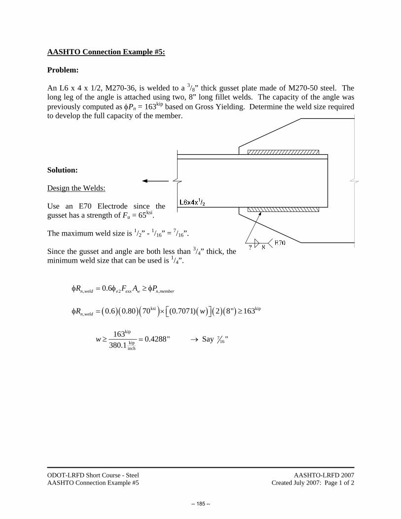
ODOT-LRFD Short Course - Steel AASHTO Connection Example #5
AASHTO-LRFD 2007 Created July 2007: Page 1 of 2
AASHTO Connection Example #5: Problem: An L6 x 4 x 1/2, M270-36, is welded to a 3/8” thick gusset plate made of M270-50 steel. The long leg of the angle is attached using two, 8” long fillet welds. The capacity of the angle was previously computed as φPn = 163kip based on Gross Yielding. Determine the weld size required to develop the full capacity of the member. Solution: Design the Welds: Use an E70 Electrode since the gusset has a strength of Fu = 65ksi. The maximum weld size is 1/2” - 1/16” = 7/16”. Since the gusset and angle are both less than 3/4” thick, the minimum weld size that can be used is 1/4”. , 2 ,0.6n weld e exx w n memberR F A Pφ = φ ≥ φ
( )( )( ) ( ) ( )( )ksi kip, 0.6 0.80 70 (0.7071) 2 8" 163n weldR wφ = × ≥⎡ ⎤⎣ ⎦
kip
716kip
inch
163 0.4288" Say "380.1
w ≥ = →
-- 185 --

ODOT-LRFD Short Course - Steel AASHTO Connection Example #5
AASHTO-LRFD 2007 Created July 2007: Page 2 of 2
Check Tension for the Gusset: Check tension on the Whitmore section: Since the overall width of the gusset is not given, I’ll check the Whitmore width assuming that it governs. If the overall width is less than the Whitmore width, these calculations will be unconservative. Compute the width of the Whitmore section: ( )( ) ( )6" 2 8" 30 15.24"wL Tan= + ° = Gross Section Yielding: ( ) ( )( )ksi kip3
8(0.95) 50 15.24" " 271.4n y gP F Aφ = φ = =⎡ ⎤⎣ ⎦
Net Section Fracture:
( ) ( )( ) ( )ksi kip38(0.80) 65 15.24" " 1.00 297.1n u eP F Aφ = φ = =⎡ ⎤⎣ ⎦ (Taking U = 1.00)
Check Block Shear in the Gusset Plate: ( ) 23
8(6") " 2.250 intg tnA A= = = ( )( ) 238(2) 8" " 6.000 invg vnA A= = =
? ?
2 2 20.58 2.250 in (0.58)(6.000 in ) 3.480 in NO!tn vnA A≥ → ≥ = 0.58n u vn y tgR F A F A∴ = + (6.13.4-2) ( )( ) ( )( )ksi 2 ksi 2 kip (0.58) 65 6.000 in 50 2.250 in 338.7nR = + =
( )kip kip(0.80) 338.7 271.0nRφ = =
Use 7/16” x 8” Fillet Welds made with an E70 Electrode
-- 186 --

ODOT-LRFD Short Course - Steel AASHTO Connection Example #6a
AASHTO-LRFD 2007 Created July 2007: Page 1 of 2
AASHTO Connection Example #6a: Problem: Use the elastic vector method to compute the maximum force on any bolt in the
eccentrically loaded bolt group shown in the figure below. The bolts are all the same size. (Example 4.12.1 from Salmon & Johnson)
B
C D
E F
P3"4"
3"3"
A
Solution:
( )( )
( )( ) ( )( ) ( )
( )( )
( ) ( )
kip k-in
2 2
2 2 22 2
4
k-in 2 2
4
ksi
2ksi kip
24 3" 2" 120
4 (2") (3") 2 2" 1"4
47.12 in
120 (2") (3")Corner Bolts:
47.12 in9.182
9.182 1" 7.2114
Tr TJ
J Ad A d
J
J
TrJ
V
τ = → = + =
= =
π⎛ ⎞⎡ ⎤= + + ⎜ ⎟⎢ ⎥⎣ ⎦ ⎝ ⎠=
+τ = =
τ =
π⎛ ⎞= =⎜ ⎟⎝ ⎠
∑ ∑
-- 187 --
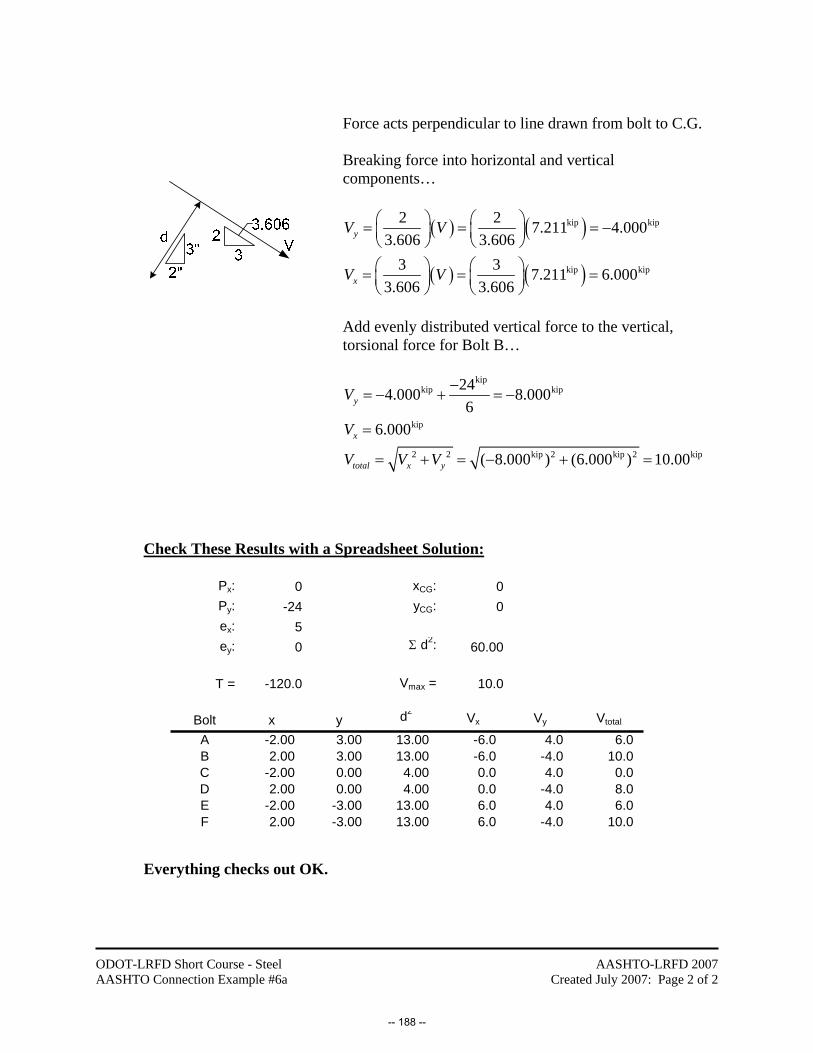
ODOT-LRFD Short Course - Steel AASHTO Connection Example #6a
AASHTO-LRFD 2007 Created July 2007: Page 2 of 2
Force acts perpendicular to line drawn from bolt to C.G. Breaking force into horizontal and vertical components…
( ) ( )
( ) ( )
kip kip
kip kip
2 2 7.211 4.0003.606 3.606
3 3 7.211 6.0003.606 3.606
y
x
V V
V V
⎛ ⎞ ⎛ ⎞= = = −⎜ ⎟ ⎜ ⎟⎝ ⎠ ⎝ ⎠⎛ ⎞ ⎛ ⎞= = =⎜ ⎟ ⎜ ⎟⎝ ⎠ ⎝ ⎠
Add evenly distributed vertical force to the vertical, torsional force for Bolt B…
kipkip kip
kip
2 2 kip 2 kip 2 kip
244.000 8.0006
6.000
( 8.000 ) (6.000 ) 10.00
y
x
total x y
V
V
V V V
−= − + = −
=
= + = − + =
Check These Results with a Spreadsheet Solution:
Px: 0 xCG: 0Py: -24 yCG: 0ex: 5ey: 0 Σ d2: 60.00
T = -120.0 Vmax = 10.0
Bolt x y d2 Vx Vy Vtotal
A -2.00 3.00 13.00 -6.0 4.0 6.0B 2.00 3.00 13.00 -6.0 -4.0 10.0C -2.00 0.00 4.00 0.0 4.0 0.0D 2.00 0.00 4.00 0.0 -4.0 8.0E -2.00 -3.00 13.00 6.0 4.0 6.0F 2.00 -3.00 13.00 6.0 -4.0 10.0
Everything checks out OK.
-- 188 --
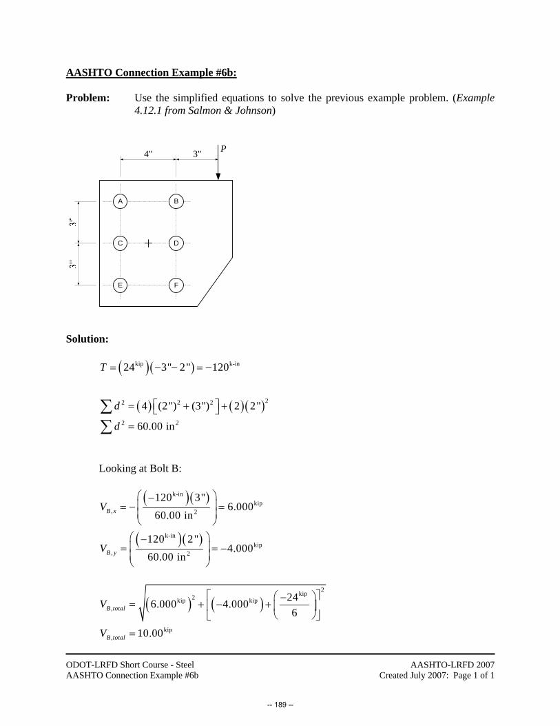
ODOT-LRFD Short Course - Steel AASHTO Connection Example #6b
AASHTO-LRFD 2007 Created July 2007: Page 1 of 1
AASHTO Connection Example #6b: Problem: Use the simplified equations to solve the previous example problem. (Example
4.12.1 from Salmon & Johnson)
B
C D
E F
P3"4"
A
Solution:
( )( )
( ) ( )( )
kip k-in
22 2 2
2 2
24 3" 2" 120
4 (2") (3") 2 2"
60.00 in
T
d
d
= − − = −
⎡ ⎤= + +⎣ ⎦=
∑∑
Looking at Bolt B:
( )( )
( )( )
k-inkip
, 2
k-inkip
, 2
120 3"6.000
60.00 in
120 2"4.000
60.00 in
B x
B y
V
V
⎛ ⎞−⎜ ⎟= − =⎜ ⎟⎝ ⎠
⎛ ⎞−⎜ ⎟= = −⎜ ⎟⎝ ⎠
( ) ( )2kip2kip kip
,
kip,
246.000 4.0006
10.00
B total
B total
V
V
⎡ ⎤⎛ ⎞−= + − +⎢ ⎥⎜ ⎟
⎝ ⎠⎣ ⎦
=
-- 189 --
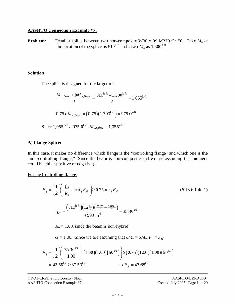
ODOT-LRFD Short Course - Steel AASHTO Connection Example #7
AASHTO-LRFD 2007 Created July 2007: Page 1 of 20
AASHTO Connection Example #7: Problem: Detail a splice between two non-composite W30 x 99 M270 Gr 50. Take Mu at
the location of the splice as 810k-ft and take φMn as 1,300k-ft.
Solution: The splice is designed for the larger of:
k-ft k-ft
, , k-ft810 1,300 1,0552 2
u Beam n BeamM M+ φ += =
( )( )k-ft k-ft
,0.75 0.75 1,300 975.0n BeamMφ = =
Since 1,055k-ft > 975.0k-ft, Mu,Splice = 1,055k-ft A) Flange Splice: In this case, it makes no difference which flange is the “controlling flange” and which one is the “non-controlling flange,” (Since the beam is non-composite and we are assuming that moment could be either positive or negative). For the Controlling flange:
1 0.75 2
cfcf f yf f yf
h
fF F F
R⎛ ⎞⎛ ⎞= + αφ ≥ αφ⎜ ⎟⎜ ⎟⎜ ⎟⎝ ⎠⎝ ⎠
(6.13.6.1.4c-1)
( )( )( )k-ft 29.7" 0.670"in
ft 2 2 ksi4
810 1235.36
3,990 incff−
= =
Rh = 1.00, since the beam is non-hybrid. α = 1.00. Since we are assuming that φMn = φMp, Fn = Fyf
( )( )( ) ( )( )( )( )
ksiksi ksi
ksi ksi ksi
1 35.36 1.00 1.00 50 0.75 1.00 1.00 502 1.00
42.68 37.50 42.68
cf
cf
F
F
⎛ ⎞⎛ ⎞= + ≥⎜ ⎟⎜ ⎟⎜ ⎟⎝ ⎠⎝ ⎠= ≥ → =
-- 190 --

ODOT-LRFD Short Course - Steel AASHTO Connection Example #7
AASHTO-LRFD 2007 Created July 2007: Page 2 of 20
For the Non-Controlling Flange:
0.75 ncfncf cf f yf
h
fF R F
R= ≥ αφ (6.13.6.1.4c-3)
ksi35.36ncf cff f= =
ksi
ksi42.68 1.20735.36
cfcf
cf
FR
f= = =
( ) ( )( )( )( )
ksiksi
ksi ksi ksi
35.361.207 0.75 1.00 1.00 501.00
42.68 37.50 42.68
ncf
ncf
F
F
= ≥
= ≥ → =
For the Compression Flange: ,u Comp cf eP F A= In compression, Ae is taken as the gross area of the flange. ( )( ) 210.5" 0.670" 7.035 ine gA A= = = ( )( )ksi 2 kip
, 42.68 7.035 in 300.3u CompP = =
For the Tension Flange: ,u Ten cf eP F A=
In tension, u ue n g
y y
FA A AF
⎛ ⎞φ= ≤⎜ ⎟⎜ ⎟φ⎝ ⎠
(6.13.6.4c-2)
For 1” diameter bolts, ( ) ( )( ) ( ) 21
810.5" 2 1 " 0.670" 5.528 innA = − =⎡ ⎤⎣ ⎦
-- 191 --

ODOT-LRFD Short Course - Steel AASHTO Connection Example #7
AASHTO-LRFD 2007 Created July 2007: Page 3 of 20
( )( )( )( ) ( )
ksi2 2
ksi
2 2 2
0.80 655.528 in 7.035 in
0.95 50
6.052 in 7.035 in 6.052 in
e
e
A
A
⎛ ⎞⎜ ⎟= ≤⎜ ⎟⎝ ⎠
= ≤ → =
( )( )ksi 2 kip
, 42.68 6.052 in 258.3u TenP = =
Proceed assuming that the flange splice will consist of plate on both the outside and inside of the flange. Assume that the flange force will be equally distributed between in the inner and outer plates (we’ll check the validity of this assumption later). Also assume that the outer splice plate will be 10.5” wide (the same width as the flange) with two rows of 1” diameter M164 (A325) bolts.
kip
kip,
258.3 129.12u TenP = =
kipkip
,300.3 150.2
2u CompP = =
For the Outer Flange Splice Plate:
Gross Yielding (Tension): ,n y y g u TenP F A Pφ = φ ≥ (6.8.2.1-1)
( )( )( )( )ksi kip0.95 50 10.5" 129.1n outerP tφ = ≥
( )( )( )
kip
ksi
516
129.10.95 50 10.5"
0.2589" say "
outert ≥
≥ →
Net Section Fracture (Tension): ,n u u n u TenP F A U Pφ = φ ≥ (6.8.2.1-2)
( )( ) ( ) ( )( ) ( )( )ksi kip180.80 65 10.5" 2 1" " 1.00 129.1n outerP tφ = − + ≥⎡ ⎤⎣ ⎦
( )( )( )
kip
ksi
516
129.10.80 65 8.25"
0.3010" say "
outert ≥
≥ →
-- 192 --
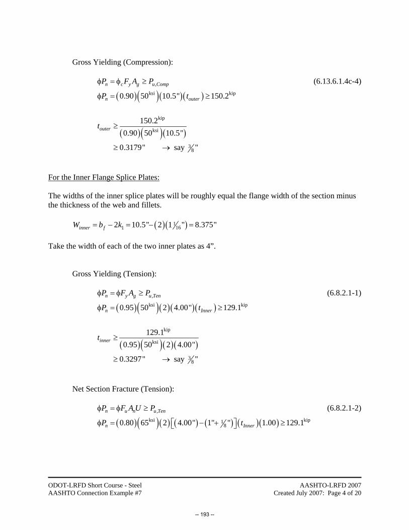
ODOT-LRFD Short Course - Steel AASHTO Connection Example #7
AASHTO-LRFD 2007 Created July 2007: Page 4 of 20
Gross Yielding (Compression): ,n c y g u CompP F A Pφ = φ ≥ (6.13.6.1.4c-4)
( )( )( )( )ksi kip0.90 50 10.5" 150.2n outerP tφ = ≥
( )( )( )
kip
ksi
38
150.20.90 50 10.5"
0.3179" say "
outert ≥
≥ →
For the Inner Flange Splice Plates: The widths of the inner splice plates will be roughly equal the flange width of the section minus the thickness of the web and fillets. ( )( )1
1612 10.5" 2 1 " 8.375"inner fW b k= − = − = Take the width of each of the two inner plates as 4”.
Gross Yielding (Tension): ,n y g u TenP F A Pφ = φ ≥ (6.8.2.1-1)
( )( )( )( )( )ksi kip0.95 50 2 4.00" 129.1n InnerP tφ = ≥
( )( )( )( )
kip
ksi
38
129.10.95 50 2 4.00"
0.3297" say "
innert ≥
≥ →
Net Section Fracture (Tension): ,n u n u TenP F A U Pφ = φ ≥ (6.8.2.1-2)
( )( )( ) ( ) ( ) ( )( )ksi kip180.80 65 2 4.00" 1" " 1.00 129.1n InnerP tφ = − + ≥⎡ ⎤⎣ ⎦
-- 193 --

ODOT-LRFD Short Course - Steel AASHTO Connection Example #7
AASHTO-LRFD 2007 Created July 2007: Page 5 of 20
( )( )( )
kip
ksi
716
129.10.80 65 5.75"
0.4318" say "
innert ≥
≥ →
Gross Yielding (Compression): ,n c y g u CompP F A Pφ = φ ≥ (6.13.6.1.4c-4)
( )( )( )( )( )ksi kip0.90 50 2 4.00" 150.2n InnerP tφ = ≥
( )( )( )( )
kip
ksi
716
150.20.90 50 2 4.00"
0.4172" say "
Innert ≥
≥ →
For a flange splice with inner and outer splice plates, the flange design force at the strength limit state may be assumed divided equally to the inner and outer plates and their connections when the areas of the inner and outer plates do not differ by more than 10% (Commentary, Page 6-191). ( )( ) 23
810.5" " 3.938 inOuterA = = ( )( )( ) 27162 4.00" " 3.500 inInnerA = =
( ) ( ) ( )( ) ( )
2 2
2 2
2 3.938 in 3.500 in11.76%
3.938 in 3.500 inOuter Inner
Ave
A AA
−−= =
+
Since the difference area is greater than 10%, either (1) the assumption that the flange force is evenly divided between the outer and inner plates must be modified, or (2) the inner plate thickness must be increased to 1/2”, which would result in a difference in area between the outer and inner plates of less than 2%. The second option will be selected for the case of this example. Outer Flange Splice Plate: 101/2” x 3/8” Inner Flange Splice Plates: 4” x 1/8”
-- 194 --
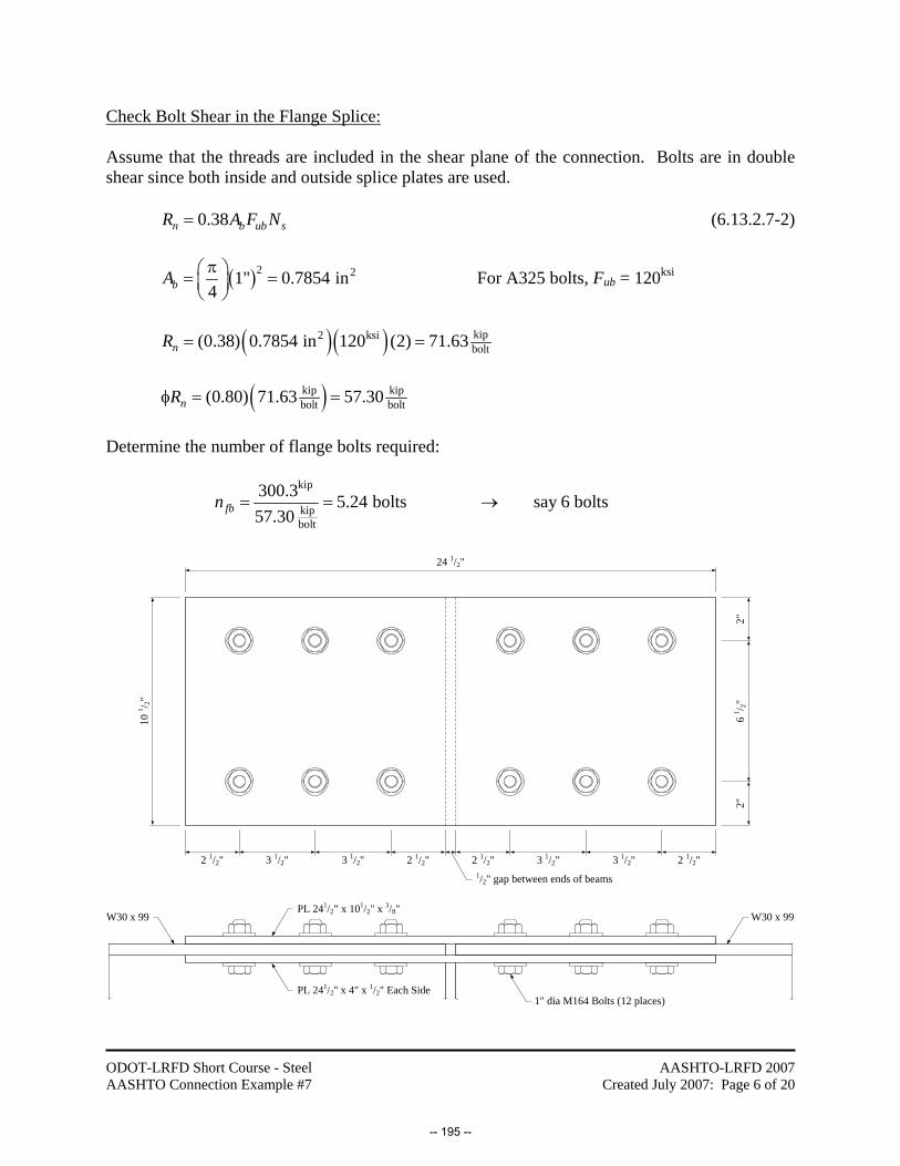
ODOT-LRFD Short Course - Steel AASHTO Connection Example #7
AASHTO-LRFD 2007 Created July 2007: Page 6 of 20
Check Bolt Shear in the Flange Splice: Assume that the threads are included in the shear plane of the connection. Bolts are in double shear since both inside and outside splice plates are used. 0.38n b ub sR A F N= (6.13.2.7-2)
( )2 21" 0.7854 in4bA π⎛ ⎞= =⎜ ⎟
⎝ ⎠ For A325 bolts, Fub = 120ksi
( )( ) kip2 ksibolt(0.38) 0.7854 in 120 (2) 71.63nR = =
( )kip kipbolt bolt(0.80) 71.63 57.30nRφ = =
Determine the number of flange bolts required:
kip
kipbolt
300.3 5.24 bolts say 6 bolts57.30fbn = = →
2 1/2" 3 1/2" 2 1/2" 2 1/2" 2 1/2"3 1/2" 3 1/2" 3 1/2"
10 1 / 2"
2"6
1 / 2"2"
1/2" gap between ends of beams
PL 241/2” x 101/2" x 3/8"
PL 241/2" x 4" x 1/2" Each Side
W30 x 99W30 x 99
1" dia M164 Bolts (12 places)
24 1/2"
-- 195 --

ODOT-LRFD Short Course - Steel AASHTO Connection Example #7
AASHTO-LRFD 2007 Created July 2007: Page 7 of 20
Check Bolt Bearing in the Flange Splice: Interior Bolts Bearing on the Beam Flange: ( )( )( )1 1 1
2 2 163 " 2 1" " 2.438"cL = − + = Since Lc = 2.433” > 2d = 2.0”, 2.4n uR dtF= ( ) ( ) kipksi
bolt(2.4) 1" (0.670") 65 104.5nR = = (6.13.2.9-1)
Interior Bolts Bearing on the Splice Plates: ( )( )( )1 1 1
2 2 163 " 2 1" " 2.438"cL = − + = Since Lc = 2.433” > 2d = 2.0”, 2.4n uR dtF= ( )( )( ) kipksi3 1
8 2 bolt(2.4) 1" " " 65 136.5nR = + = (6.13.2.9-1)
End Bolts Bearing on the Beam Flange: ( )( )1 1 1
2 2 162 " 1" " 1.969"cL = − + = Since Lc = 1.969” < 2d = 2.0”, 1.2n c uR L tF= ( ) ( ) kipksi
bolt(1.2) 1.969" (0.670") 65 102.9nR = = (6.13.2.9-2)
End Bolts Bearing on the Splice Plates: ( )( )1 1 1
2 2 162 " 1" " 1.969"cL = − + = Since Lc = 1.969” < 2d = 2.0”, 1.2n c uR L tF= ( )( )( ) kipksi3 1
8 2 bolt(1.2) 1.969" " " 65 134.4nR = + = (6.13.2.9-2)
For all 6 Bolts: ( ) ( ) ( )kip kip kip kip
bolt bolt bolt(2 bolts) 104.5 (2 bolts) 104.5 (2 bolts) 102.9 623.9nR = + + =
( )kip kip(0.80) 623.9 499.1nRφ = = OK
-- 196 --

ODOT-LRFD Short Course - Steel AASHTO Connection Example #7
AASHTO-LRFD 2007 Created July 2007: Page 8 of 20
Check Slip of the Flange Splice: Bolted connections for flange splices shall be designed as slip-critical connections for the flange design force. As a minimum, for checking slip of the flange splice bolts, the design force for the flange under consideration shall be taken as the Service II design stress, Fs, times the smaller gross flange area on either side of the splice. Take the Service II moment as 548k-ft
slip s gP F A= where ( )( )( )
( )( )k-ft 29.7" 0.670"in
ft 2 2 ksi4
548 1223.92
1.00 3,990 ins
sh
fFR
−= = = (6.13.6.1.4c-5)
( )( )( )ksi kip23.92 10.5" 0.670" 168.3slipP = =
The slip resistance of a single bolt is taken as: n h s s tR K K N P= (6.13.2.8-1)
Kh = 1.00 (for standard holes) Ks = 0.33 (assume Class A surface) Ns = 2 Pt = 51kip (from Table 6.13.2.8-1 for M164 Bolts)
( ) kipkip
bolt(1.00)(0.33)(2) 51 33.66nR = =
Determine the number of flange bolts required:
kip
kipbolt
168.3 5.00 bolts 6 bolts will work33.66fbn = = →
-- 197 --

ODOT-LRFD Short Course - Steel AASHTO Connection Example #7
AASHTO-LRFD 2007 Created July 2007: Page 9 of 20
Check Block Shear of the Beam Flange:
( )( )( ) 22 2" 0.670" 2.680 intgA = =
( ) ( )( ) ( ) 21 1822 2" 1" " 0.670" 1.926 intnA ⎡ ⎤= − + =⎣ ⎦
( )( )( ) 21 1 1
2 2 22 3 " 3 " 2 " 0.670" 12.73 invgA = + + =
( ) ( )( ) ( ) 21 12 82 9 " 2.5 1" " 0.670" 8.961 invnA = − + =⎡ ⎤⎣ ⎦
?
?2 2 2
0.58
1.926 in (0.58)(8.961 in ) 5.198 in NO!
tn vnA A≥
≥ =
0.58n u vn y tgR F A F A∴ = + (6.13.4-2) ( )( ) ( )( )ksi 2 ksi 2 kip (0.58) 65 8.961 in 50 2.680 in 471.8nR = + =
( )kip kip(0.80) 471.8 377.5nRφ = = OK
3 1/2" 2 1/2"3 1/2"
2"6
1 / 2"2"
Shear
Shear
Tens
ion
-- 198 --
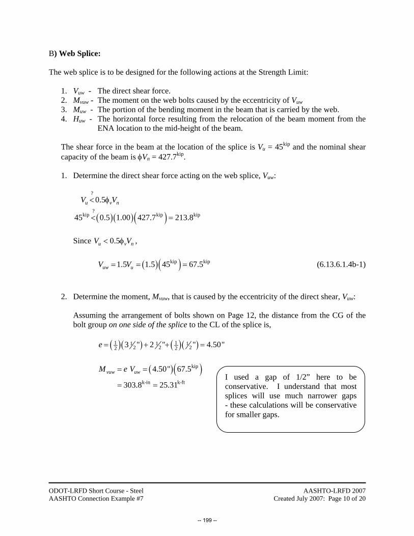
ODOT-LRFD Short Course - Steel AASHTO Connection Example #7
AASHTO-LRFD 2007 Created July 2007: Page 10 of 20
B) Web Splice: The web splice is to be designed for the following actions at the Strength Limit:
1. Vuw - The direct shear force. 2. Mvuw - The moment on the web bolts caused by the eccentricity of Vuw 3. Muw - The portion of the bending moment in the beam that is carried by the web. 4. Huw - The horizontal force resulting from the relocation of the beam moment from the
ENA location to the mid-height of the beam.
The shear force in the beam at the location of the splice is Vu = 45kip and the nominal shear capacity of the beam is φVn = 427.7kip.
1. Determine the direct shear force acting on the web splice, Vuw:
( )( )( )
?
?kip kip kip
0.5
45 0.5 1.00 427.7 213.8
u v nV V< φ
< =
Since 0.5u v nV V< φ , ( )( )kip kip1.5 1.5 45 67.5uw uV V= = = (6.13.6.1.4b-1)
2. Determine the moment, Mvuw, that is caused by the eccentricity of the direct shear, Vuw:
Assuming the arrangement of bolts shown on Page 12, the distance from the CG of the bolt group on one side of the splice to the CL of the splice is,
( )( ) ( )( )1 11 1 1
2 2 22 23 " 2 " " 4.50"e = + + =
( )( )kip
k-in k-ft
4.50" 67.5
303.8 25.31
vuw uwM e V= =
= = I used a gap of 1/2” here to be
conservative. I understand that most splices will use much narrower gaps - these calculations will be conservative for smaller gaps.
-- 199 --
ODOT-LRFD Short Course - Steel AASHTO Connection Example #7
AASHTO-LRFD 2007 Created July 2007: Page 11 of 20
3. Determine the portion of the beam moment that is carried by the web splice, Muw:
2
12w
uw h cf cf ncft DM R F R f= − (C6.13.6.1.4b-1)
ksi42.68cfF = (Positive since it’s in tension) 1.207cfR = (from Before) ksi35.36ncff = − (Negative since it’s in compression)
( )( ) ( )( ) ( )( )
( )
2ksi ksi
3 ksi k-in k-ft
0.520" 28.36"1.00 42.08 1.207 35.36
12
34.85 in 85.36 2,975 247.9
uwM⎡ ⎤
= − −⎢ ⎥⎢ ⎥⎣ ⎦
= = =
4. Determine the horizontal force that results from moving the beam moment, Huw:
12w
uw h cf cf ncft DH R F R f= + (C6.13.6.1.4b-2)
( )( ) ( )( ) ( )( )
( )
ksi ksi
2 ksi kip
0.520" 28.36"1.00 42.68 1.207 35.36
12
1.229 in 0.000 0.00
uwH⎡ ⎤
= + −⎢ ⎥⎣ ⎦
= =
In this case, the ENA is at the mid-height of the beam. Since Huw is the horizontal force that results from the eccentricity of the ENA relative to the mid-height of the beam, it makes sense that Huw is zero.
-- 200 --
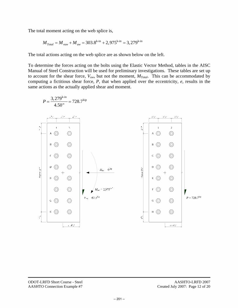
ODOT-LRFD Short Course - Steel AASHTO Connection Example #7
AASHTO-LRFD 2007 Created July 2007: Page 12 of 20
The total moment acting on the web splice is, k-in k-in k-in303.8 2,975 3, 279Total vuw uwM M M= + = + = The total actions acting on the web splice are as shown below on the left. To determine the forces acting on the bolts using the Elastic Vector Method, tables in the AISC Manual of Steel Construction will be used for preliminary investigations. These tables are set up to account for the shear force, Vuw, but not the moment, MTotal. This can be accommodated by computing a fictitious shear force, P, that when applied over the eccentricity, e, results in the same actions as the actually applied shear and moment.
k-in
kip3, 279 728.74.50"
P = =
P = 728.7kip
A
B
C
D
E
F
G
H
1 2
2 1/2" 3 1/2" 2 3/4"
e = 41/2"
-- 201 --
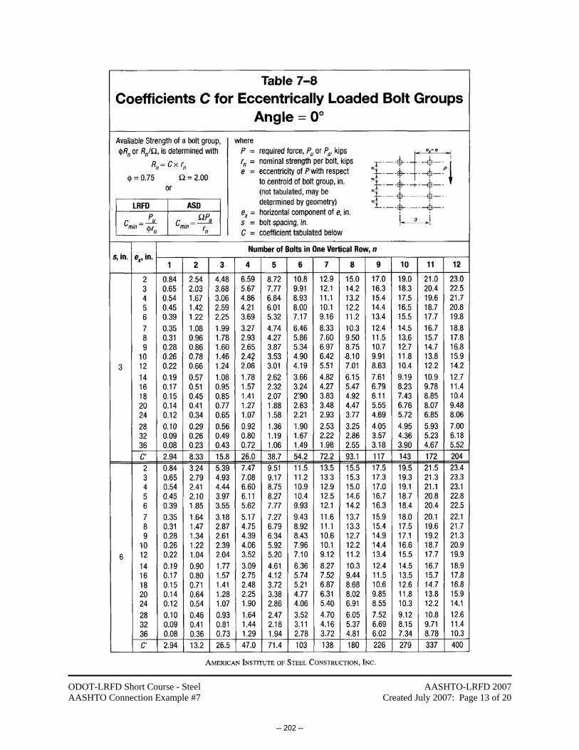
ODOT-LRFD Short Course - Steel AASHTO Connection Example #7
AASHTO-LRFD 2007 Created July 2007: Page 13 of 20
-- 202 --

ODOT-LRFD Short Course - Steel AASHTO Connection Example #7
AASHTO-LRFD 2007 Created July 2007: Page 14 of 20
From Table 7-8 on Page 7-38 of the 13th Ed. of the AISC Manual of Steel Construction,
kip
min kipbolt
728.7 12.7257.30
u
n
PCr
= = =φ
From the Table for e = 4.00”, S = 3.00”, and for 8 bolts in a row, C = 13.2 From the Table for e = 5.00”, S = 3.00”, and for 8 bolts in a row, C = 12.2 The average of these two values is 12.7. Although this is slightly smaller than 12.72, the proposed configuration will probably still work since our horizontal spacing is 31/2” instead of 3”. Elastic Vector Method for the Web Splice:
( ) ( )( ) ( ) ( ) ( ) ( )( ) ( )( ) ( ) ( ) ( ) ( )
2 2 2 222, , , ,
2 2 2 2 22 2
4 4
4 4 1.75" 1.5" 4.5" 7.5" 10.5" 805 in
x y D y C y B y Ad d d d d d
d
⎡ ⎤Σ = + + + +⎢ ⎥⎣ ⎦⎡ ⎤Σ = + + + + =⎣ ⎦
Examine Bolt A2:
( )( )k-in
kip, 2 2
3, 279 10.5" 42.77805 inT X
T yVd
= = =Σ
( )( )k-in
kip, 2 2
3, 279 1.75" x 7.128805 inT Y
TVd
= = =Σ
The direct shear force is,
( )kip
kip, bolt
67.54.219
16 boltsD YV = =
( ) ( )2 2kip kip kip kip42.77 7.128 4.219 44.25TotalV = + + =
From this, an actual value of C can be computed, which will be useful when investigating slip resistance.
kip
kipbolt
728.7 16.4744.25
TotalActual
bolt
PCP
= = =
-- 203 --

ODOT-LRFD Short Course - Steel AASHTO Connection Example #7
AASHTO-LRFD 2007 Created July 2007: Page 15 of 20
The calculations shown on the previous page have been validated using the spreadsheet shown here.
M: 2975Px: 0 xCG: 0Py: 67.5 yCG: 0ex: 4.5ey: 0 Σ d2: 805.00
T = 3278.75 Vmax = 44.2459
Bolt x y d2 Vx Vy Vtotal
A1 -1.75 10.50 113.31 42.7663 -7.1277 42.8651B1 -1.75 7.50 59.31 30.5474 -7.1277 30.6856C1 -1.75 4.50 23.31 18.3284 -7.1277 18.5578D1 -1.75 1.50 5.31 6.1095 -7.1277 6.7667E1 -1.75 -1.50 5.31 -6.1095 -7.1277 6.7667F1 -1.75 -4.50 23.31 -18.3284 -7.1277 18.5578G1 -1.75 -7.50 59.31 -30.5474 -7.1277 30.6856H1 -1.75 -10.50 113.31 -42.7663 -7.1277 42.8651A2 1.75 10.50 113.31 42.7663 7.1277 44.2459B2 1.75 7.50 59.31 30.5474 7.1277 32.5866C2 1.75 4.50 23.31 18.3284 7.1277 21.5563D2 1.75 1.50 5.31 6.1095 7.1277 12.8867E2 1.75 -1.50 5.31 -6.1095 7.1277 12.8867F2 1.75 -4.50 23.31 -18.3284 7.1277 21.5563G2 1.75 -7.50 59.31 -30.5474 7.1277 32.5866H2 1.75 -10.50 113.31 -42.7663 7.1277 44.2459
-- 204 --

ODOT-LRFD Short Course - Steel AASHTO Connection Example #7
AASHTO-LRFD 2007 Created July 2007: Page 16 of 20
Check Flexural Yielding of the Web Splice Plates: Take Muw = 3,262k-in
( )( ) 23
12 322
py
p pp p
M dM y M FI d td t
⎡ ⎤ ⎛ ⎞⎢ ⎥σ = = = ≤ φ⎜ ⎟⎢ ⎥ ⎝ ⎠⎣ ⎦
Solve for tp: ( )( )
( ) ( )( )k-in
2 2 ksi
3 3,2623 0.2787"26.5" 1.00 50
pp y
Mtd F
≥ = =φ
Use one PL261/2” x 171/2” x 5/16” each side of web. Check Shear Yielding of the Web Splice Plates: Take Vuw = 67.5kip
( )( )( )( )( )
( )( )( ) ( )( ) ( )ksi kip516
0.58 2
1.00 0.58 26.5" 2 " 50 480.3 OK
uw n p p yV V d t F≤ φ = φ
= =⎡ ⎤⎣ ⎦
Check Shear Rupture of the Web Splice Plates: Take Vuw = 67.5kip
( )( )( )( )( )
( )( ) ( ) ( )( ) ( )( ) ( ),
ksi kip518 16
0.58 2
0.80 0.58 26.5" 8 1 " 2 " 65 329.9 OK
uw n p net p uV V d t F≤ φ = φ
= − =⎡ ⎤ ⎡ ⎤⎣ ⎦ ⎣ ⎦
-- 205 --

ODOT-LRFD Short Course - Steel AASHTO Connection Example #7
AASHTO-LRFD 2007 Created July 2007: Page 17 of 20
Check Bearing of the Bolts in the Web Splice: Edge Bolts Bearing on the Beam Web: ( )( )1 1 1
2 2 162 " 1" " 1.969"cL = − + = Since Lc = 1.969” < 2d = 2.0”, 1.2n c uR L tF= ( ) ( ) kipksi
bolt(1.2) 1.969" (0.520") 65 79.85nR = = (6.13.2.9-2)
Edge Bolts Bearing on the Splice Plates: ( )( )1 1 1
2 2 162 " 1" " 1.969"cL = − + = Since Lc = 1.969” < 2d = 2.0”, 1.2n c uR L tF= ( )( )( )( ) kipksi5
16 bolt(1.2) 1.969" 2 " 65 95.99nR = = (6.13.2.9-2)
Summary of Splice Plate Bearing: Bearing on the beam web governs.
( )( )
kipbolt
kip kipbolt bolt
79.85
0.80 79.85 63.88 OK
n
n
R
R
=
φ = =
-- 206 --

ODOT-LRFD Short Course - Steel AASHTO Connection Example #7
AASHTO-LRFD 2007 Created July 2007: Page 18 of 20
Check Slip of the Bolts in the Web Splice: Take the Service II moment as 548k-ft. From the slip check on the flange splice, Fs and fs were determined to be 23.92ksi and Pslip was determined to be 168.3kip. Take the Service II shear force at the location of the splice to be Vsw = 30.4kip. The web splice is to be designed for the following actions at the Service II Limit
1. Vsw - The direct shear force. 2. Mvsw - The moment on the web bolts caused by the eccentricity of Vsw 3. Msw - The portion of the bending moment in the beam that is carried by the web. 4. Hsw - The horizontal force resulting from the relocation of the beam moment from the
ENA location to the mid-height of the beam.
1. The direct shear force acting on the web splice is given as, Vsw = 30.4kip:
2. Determine the moment, Mvsw, that is caused by the eccentricity of the direct shear, Vsw:
Assuming the arrangement of bolts shown on Page 12, the distance from the CG of the bolt group on one side of the splice to the CL of the splice is,
( )( ) ( )( )1 11 1 1
2 2 22 23 " 2 " " 4.50"e = + + =
( )( )kip
k-in k-ft
4.50" 30.4
136.8 11.40
vsw swM e V= =
= =
-- 207 --
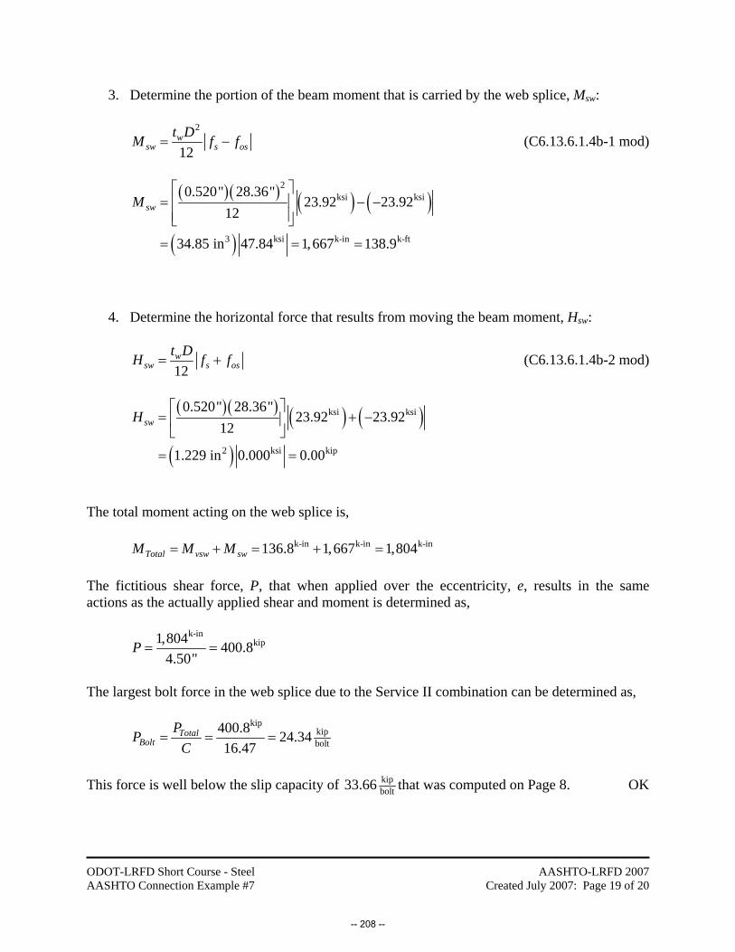
ODOT-LRFD Short Course - Steel AASHTO Connection Example #7
AASHTO-LRFD 2007 Created July 2007: Page 19 of 20
3. Determine the portion of the beam moment that is carried by the web splice, Msw:
2
12w
sw s ost DM f f= − (C6.13.6.1.4b-1 mod)
( )( ) ( ) ( )
( )
2ksi ksi
3 ksi k-in k-ft
0.520" 28.36"23.92 23.92
12
34.85 in 47.84 1,667 138.9
swM⎡ ⎤
= − −⎢ ⎥⎢ ⎥⎣ ⎦
= = =
4. Determine the horizontal force that results from moving the beam moment, Hsw:
12w
sw s ost DH f f= + (C6.13.6.1.4b-2 mod)
( )( ) ( ) ( )
( )
ksi ksi
2 ksi kip
0.520" 28.36"23.92 23.92
12
1.229 in 0.000 0.00
swH⎡ ⎤
= + −⎢ ⎥⎣ ⎦
= =
The total moment acting on the web splice is, k-in k-in k-in136.8 1,667 1,804Total vsw swM M M= + = + = The fictitious shear force, P, that when applied over the eccentricity, e, results in the same actions as the actually applied shear and moment is determined as,
k-in
kip1,804 400.84.50"
P = =
The largest bolt force in the web splice due to the Service II combination can be determined as,
kip
kipbolt
400.8 24.3416.47
TotalBolt
PPC
= = =
This force is well below the slip capacity of kip
bolt33.66 that was computed on Page 8. OK
-- 208 --
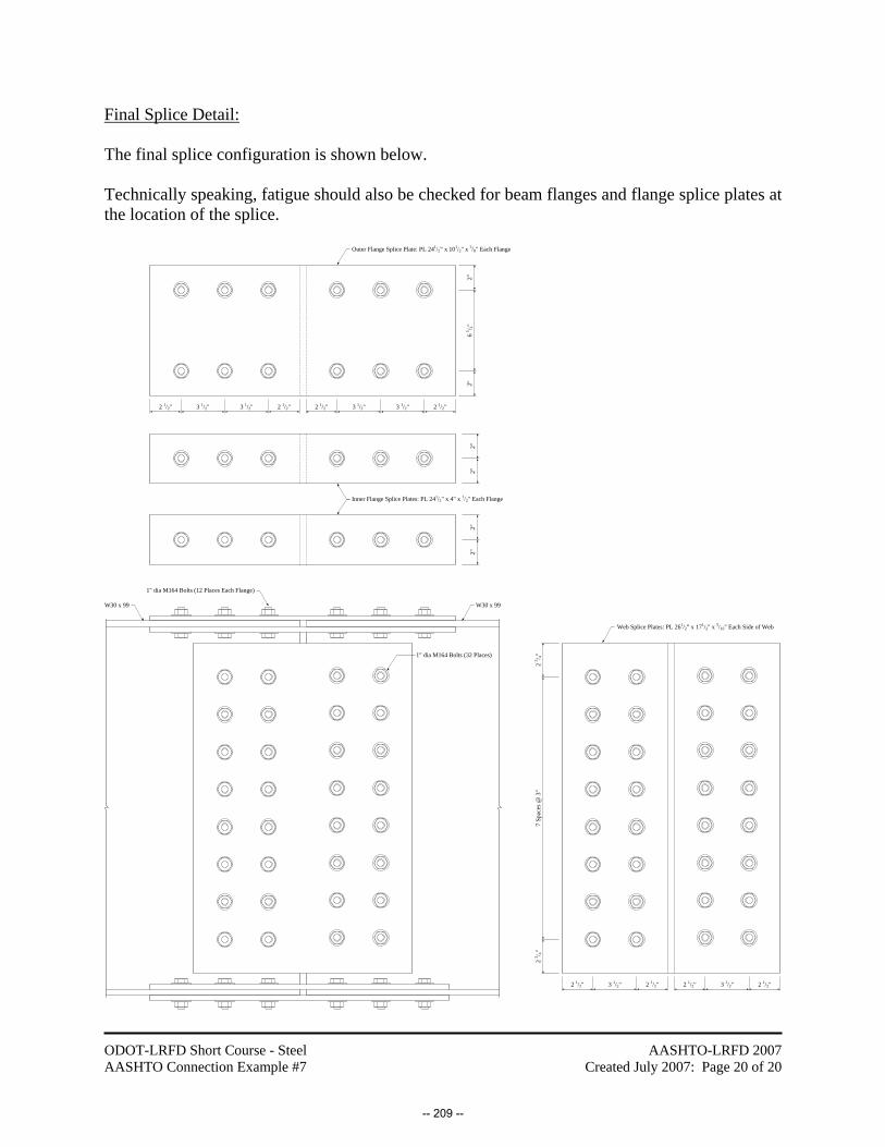
ODOT-LRFD Short Course - Steel AASHTO Connection Example #7
AASHTO-LRFD 2007 Created July 2007: Page 20 of 20
Final Splice Detail: The final splice configuration is shown below. Technically speaking, fatigue should also be checked for beam flanges and flange splice plates at the location of the splice.
2 1/2" 3 1/2" 2 1/2" 2 1/2" 2 1/2"3 1/2" 3 1/2" 3 1/2"
2"6
1 / 2"2"
2 1/2" 2 1/2"3 1/2" 2 1/2" 2 1/2"3 1/2"
2 3 / 4"
2 3 / 4"
7 Sp
aces
@ 3
"
2"2"
2"2"
Outer Flange Splice Plate: PL 241/2” x 101/2" x 3/8" Each Flange
Inner Flange Splice Plates: PL 241/2" x 4" x 1/2" Each Flange
1" dia M164 Bolts (12 Places Each Flange)
1" dia M164 Bolts (32 Places)
Web Splice Plates: PL 261/2” x 171/2" x 5/16" Each Side of Web
W30 x 99 W30 x 99
-- 209 --


![AASHTO - LRFD [Design Example for Steel Girder Superstructure Bridge - 2003]](https://static.fdocuments.in/doc/165x107/54faee334a79590b398b4fd6/aashto-lrfd-design-example-for-steel-girder-superstructure-bridge-2003.jpg)