LRFD Software for Design and Actual Ultimate Capacity of … · ii Form DOT F 1700.7 (8-72) 1...
220
A cooperative transportation research program between Kansas Department of Transportation, Kansas State University Transportation Center, and The University of Kansas Report No. K-TRAN: KSU-11-3 ▪ FINAL REPORT▪ April 2013 LRFD Software for Design and Actual Ultimate Capacity of Confined Rectangular Columns Ahmed Mohsen ABD El Fattah, Ph.D., LEED AP Hayder Rasheed, Ph.D., P.E. Asad Esmaeily, Ph.D., P.E. Kansas State University Transportation Center
Transcript of LRFD Software for Design and Actual Ultimate Capacity of … · ii Form DOT F 1700.7 (8-72) 1...

A cooperative transportation research program betweenKansas Department of Transportation,Kansas State University Transportation Center, andThe University of Kansas
Report No. K-TRAN: KSU-11-3 ▪ FINAL REPORT▪ April 2013
LRFD Software for Design and Actual Ultimate Capacity of Confined Rectangular Columns
Ahmed Mohsen ABD El Fattah, Ph.D., LEED AP Hayder Rasheed, Ph.D., P.E.Asad Esmaeily, Ph.D., P.E.
Kansas State University Transportation Center

i
This page intentionally left blank.

ii
Form DOT F 1700.7 (8-72)
1 Report No.
K-TRAN: KSU-11-3 2 Government Accession No.
3 Recipient Catalog No.
4 Title and Subtitle
LRFD Software for Design and Actual Ultimate Capacity of Confined Rectangular Columns 5 Report Date
April 2013 6 Performing Organization Code
7 Author(s)
Ahmed Mohsen ABD El Fattah, Ph.D., LEED AP; Hayder Rasheed, Ph.D., P.E.; Asad Esmaeily, Ph.D., P.E.
8 Performing Organization Report No.
9 Performing Organization Name and Address
Department of Civil Engineering Kansas State University Transportation Center 2118 Fiedler Hall Manhattan, Kansas 66506
10 Work Unit No. (TRAIS)
11 Contract or Grant No.
C1880
12 Sponsoring Agency Name and Address
Kansas Department of Transportation Bureau of Materials and Research 700 SW Harrison Street Topeka, Kansas 66603-3745
13 Type of Report and Period Covered
Final Report October 2010–September 2012
14 Sponsoring Agency Code
RE-0546-01
15 Supplementary Notes
For more information write to address in block 9.
The analysis of concrete columns using unconfined concrete models is a well established practice. On the other hand, prediction of the actual ultimate capacity of confined concrete columns requires specialized nonlinear analysis. Modern codes and standards are introducing the need to perform extreme event analysis. There has been a number of studies that focused on the analysis and testing of concentric columns or cylinders. This case has the highest confinement utilization since the entire section is under confined compression. On the other hand, the augmentation of compressive strength and ductility due to full axial confinement is not applicable to pure bending and combined bending and axial load cases simply because the area of effective confined concrete in compression is reduced. The higher eccentricity causes smaller confined concrete region in compression yielding smaller increase in strength and ductility of concrete. Accordingly, the ultimate confined strength is gradually reduced from the fully confined value fcc (at zero eccentricity) to the unconfined value f’c (at infinite eccentricity) as a function of the compression area to total area ratio. The higher the eccentricity, the smaller the confined concrete compression zone. This paradigm is used to implement adaptive eccentric model utilizing the well known Mander Model.
Generalization of the moment of area approach is utilized based on proportional loading, finite layer procedure and the secant stiffness approach, in an iterative incremental numerical model to achieve equilibrium points of P- and M- response up to failure. This numerical analysis is adapted to assess the confining effect in rectangular columns confined with conventional lateral steel. This model is validated against experimental data found in literature. The comparison shows good correlation. Finally computer software is developed based on the non-linear numerical analysis. The software is equipped with an elegant graphics interface that assimilates input data, detail drawings, capacity diagrams and demand point mapping in a single sheet. Options for preliminary design, section and reinforcement selection are seamlessly integrated as well. The software generates 3D failure surface for rectangular columns and allows the user to determine the 2D interaction diagrams for any angle between the x-axis and the resultant moment. Improvements to KDOT Bridge Design Manual using this software with reference to AASHTO LRFD are made. This study is limited to stub columns.
17 Key Words
Software, Columns, Bridge, Certified Reinforced Concrete, LRFD, Load and Resistance Factor Design
18 Distribution Statement
No restrictions. This document is available to the public through the National Technical Information Service www.ntis.gov.
19 Security Classification (of this
report)
Unclassified
20 Security Classification (of this
page) Unclassified 21 No. of pages
220 22 Price

iii
LRFD Software for Design and Actual Ultimate Capacity of Confined
Rectangular Columns
Final Report
Prepared by
Ahmed Mohsen ABD El Fattah, Ph.D., LEED AP
Hayder Rasheed, Ph.D., P.E.
Asad Esmaeily, Ph.D., P.E.
Kansas State University Transportation Center
A Report on Research Sponsored by
THE KANSAS DEPARTMENT OF TRANSPORTATION TOPEKA, KANSAS
and
KANSAS STATE UNIVERSITY TRANSPORTATION CENTER
MANHATTAN, KANSAS
April 2013
© Copyright 2013, Kansas Department of Transportation

iv
PREFACE The Kansas Department of Transportation’s (KDOT) Kansas Transportation Research and New-Developments (K-TRAN) Research Program funded this research project. It is an ongoing, cooperative and comprehensive research program addressing transportation needs of the state of Kansas utilizing academic and research resources from KDOT, Kansas State University and the University of Kansas. Transportation professionals in KDOT and the universities jointly develop the projects included in the research program.
NOTICE The authors and the state of Kansas do not endorse products or manufacturers. Trade and manufacturers names appear herein solely because they are considered essential to the object of this report. This information is available in alternative accessible formats. To obtain an alternative format, contact the Office of Transportation Information, Kansas Department of Transportation, 700 SW Harrison, Topeka, Kansas 66603-3754 or phone (785) 296-3585 (Voice) (TDD).
DISCLAIMER The contents of this report reflect the views of the authors who are responsible for the facts and accuracy of the data presented herein. The contents do not necessarily reflect the views or the policies of the state of Kansas. This report does not constitute a standard, specification or regulation.
v
Abstract
The analysis of concrete columns using unconfined concrete models is a well established
practice. On the other hand, prediction of the actual ultimate capacity of confined concrete
columns requires specialized nonlinear analysis. Modern codes and standards are introducing the
need to perform extreme event analysis. There has been a number of studies that focused on the
analysis and testing of concentric columns or cylinders. This case has the highest confinement
utilization since the entire section is under confined compression. On the other hand, the
augmentation of compressive strength and ductility due to full axial confinement is not
applicable to pure bending and combined bending and axial load cases simply because the area
of effective confined concrete in compression is reduced. The higher eccentricity causes smaller
confined concrete region in compression yielding smaller increase in strength and ductility of
concrete. Accordingly, the ultimate confined strength is gradually reduced from the fully
confined value fcc (at zero eccentricity) to the unconfined value f ’c (at infinite eccentricity) as a
function of the compression area to total area ratio. The higher the eccentricity, the smaller the
confined concrete compression zone. This paradigm is used to implement adaptive eccentric
model utilizing the well known Mander Model.
Generalization of the moment of area approach is utilized based on proportional loading,
finite layer procedure and the secant stiffness approach, in an iterative incremental numerical
model to achieve equilibrium points of P- and M- response up to failure. This numerical
analysis is adapted to assess the confining effect in rectangular columns confined with
conventional lateral steel. This model is validated against experimental data found in literature.
The comparison shows good correlation. Finally computer software is developed based on the
non-linear numerical analysis. The software is equipped with an elegant graphics interface that
assimilates input data, detail drawings, capacity diagrams and demand point mapping in a single
sheet. Options for preliminary design, section and reinforcement selection are seamlessly
integrated as well. The software generates 3D failure surface for rectangular columns and allows
the user to determine the 2D interaction diagrams for any angle between the x-axis and the
resultant moment. Improvements to KDOT Bridge Design Manual using this software with
reference to AASHTO LRFD are made. This study is limited to stub columns.

vi
Table of Contents
Abstract .......................................................................................................................................... v
Table of Contents ......................................................................................................................... vi
List of Figures .............................................................................................................................. vii
List of Tables .............................................................................................................................. xiii
Acknowledgements .................................................................................................................... xiv
Chapter 1: Introduction ............................................................................................................... 1
1.1 Background ..................................................................................................................... 1
1.2 Objectives ....................................................................................................................... 1
1.3 Scope ............................................................................................................................... 2
Chapter 2: Literature Review ...................................................................................................... 4
2.1 Steel Confinement Models .............................................................................................. 4
2.1.1 Chronological Review of Models ............................................................................... 4
2.1.2 Discussion ................................................................................................................. 50
2.2 Rectangular Columns Subjected to Biaxial Bending and Axial Compression ............. 55
2.2.1 Past Work Review..................................................................................................... 56
2.2.2 Discussion ............................................................................................................... 109
Chapter 3: Rectangular Columns Subjected to Biaxial Bending and Axial Compression 111
3.1 Introduction ................................................................................................................. 111
3.2 Unconfined Rectangular Columns Analysis ............................................................... 112
3.2.1 Formulations ........................................................................................................... 112
3.2.2 Analysis Approaches .............................................................................................. 114
3.2.3 Results and Discussion ........................................................................................... 131
3.3 Confined Rectangular Columns Analysis ................................................................... 136
3.3.1 Formulations ........................................................................................................... 136
3.3.2 Numerical Formulation ........................................................................................... 160
3.3.3 Results and Discussion ........................................................................................... 170
Chapter 4: Conclusions and Recommendations .................................................................... 186
4.1 Conclusions ................................................................................................................. 186
4.2 Recommendations ....................................................................................................... 186
References .................................................................................................................................. 188
Appendix A: Ultimate Confined Strength Tables .................................................................. 197

vii
List of Figures
FIGURE 2.1 General Stress-Strain Curve by Chan (1955) ............................................................ 6
FIGURE 2.2 General Stress-Strain Curve by Blume et al. (1961) ................................................. 7
FIGURE 2.3 General Stress-Strain Curve by Soliman and Yu (1967) ........................................... 9
FIGURE 2.4 Stress-Strain Curve by Kent and Park (1971) ......................................................... 11
FIGURE 2.5 Stress-Strain Curve by Vallenas et al. (1977). ........................................................ 13
FIGURE 2.6 Proposed Stress-Strain Curve by Wang et al. (1978) .............................................. 15
FIGURE 2.7 Proposed Stress-Strain Curve by Muguruma et al. (1980) ...................................... 17
FIGURE 2.8 Proposed General Stress-Strain Curve by Sheikh and Uzumeri (1982) .................. 20
FIGURE 2.9 Proposed General Stress-Strain Curve by Park et al. (1982) ................................... 22
FIGURE 2.10 Proposed General Stress-Strain Curve by Yong et al. (1988) ............................... 25
FIGURE 2.11 Stress-Strain Model Proposed by Mander et al. (1988) ........................................ 27
FIGURE 2.12 Proposed General Stress-Strain Curve by Fujii et al. (1988) ................................ 29
FIGURE 2.13 Proposed Stress-Strain Curve by Saatcioglu and Razvi (1992-1999) ................... 31
FIGURE 2.14 Proposed Stress-Strain Curve by Cusson and Paultre (1995) ............................... 37
FIGURE 2.15 Proposed Stress-Strain Curve by Attard and Setunge (1996) ............................... 40
FIGURE 2.16 Mander et al. (1988), Saatcioglu and Razvi (1992) and El-Dash and Ahmad
(1995) Models Compared to Case 1 ..................................................................................... 54
FIGURE 2.17 Mander et al. (1988), Saatcioglu and Razvi (1992) and El-Dash and Ahmad
(1995) Models Compared to Case 2 ..................................................................................... 54
FIGURE 2.18 Mander et al. (1988), Saatcioglu and Razvi (1992) and El-Dash and Ahmad
(1995) Models Compared to Case 3 ..................................................................................... 55
FIGURE 2.19 Relation between T and C by Andersen (1941) .................................................... 59
FIGURE 2.20 Relation between c and byBakhoum (1948) ..................................................... 61
FIGURE 2.21 Geometric Dimensions in Crevin Analysis (1948) ............................................... 63
viii
FIGURE 2.22 Concrete Center of Pressure versus Neutral Axis Location, Mikhalkin 1952 ...... 64
FIGURE 2.23 Steel Center of Pressure versus Neutral Axis Location, Mikhalkin 1952 ............. 64
FIGURE 2.24 Bending with Normal Compressive Force Chart np = 0.03, Hu (1955). In His
Paper the Graphs Were Plotted with Different Values of np 0.03,0.1 ,0.3 .......................... 66
FIGURE 2.25 Linear Relationship between Axial Load and Moment for Compression Failure
Whitney and Cohen 1957 ...................................................................................................... 70
FIGURE 2.26 Section and Design Chart for Case 1(rx/b = 0.005), Au (1958) ............................ 72
FIGURE 2.27 Section and Design Chart for Case 2, Au (1958) .................................................. 72
FIGURE 2.28 Section and Design Chart for Case 3(dx/b = 0.7, dy/t = 0. 7), Au (1958) .............. 73
FIGURE 2.29 Graphical Representation of Method One by Bresler (1960) ................................ 77
FIGURE 2.30 Graphical Representation of Method Two by Bresler (1960) ............................... 78
FIGURE 2.31 Interaction Curves Generated from Equating and by Bresler (1960) ................ 78
FIGURE 2.32 Five Cases for the Compression Zone Based on the Neutral Axis Location
Czerniak (1962) .................................................................................................................... 80
FIGURE 2.33 Values for N for Unequal Steel Distribution by Pannell (1963) ........................... 84
FIGURE 2.34 Design Curve by Fleming et al. (1961) ................................................................. 86
FIGURE 2.35 Relation between and by Ramamurthy (1966) ............................................... 88
FIGURE 2.36 Biaxial Moment Relationship by Parme et al. (1966) ........................................... 89
FIGURE 2.37 Biaxial Bending Design Constant (Four Bars Arrangement) by Parme et al. (1966)
............................................................................................................................................... 89
FIGURE 2.38 Biaxial Bending Design Constant (Eight Bars Arrangement) by Parme et al.
(1966) .................................................................................................................................... 90
FIGURE 2.39 Biaxial Bending Design Constant (Twelve Bars Arrangement) by Parme et al.
(1966) .................................................................................................................................... 90
FIGURE 2.40 Biaxial Bending Design Constant (6-8-10 Bars Arrangement) by Parme et al.
(1966) .................................................................................................................................... 91

ix
FIGURE 2.41 Simplified Interaction Curve by Parme et al. (1966) ............................................ 92
FIGURE 2.42 Working Stress Interaction Diagram for Bending about X-Axis by Mylonas
(1967) .................................................................................................................................... 93
FIGURE 2.43 Comparison of Steel Stress Variation for Biaxial Vending When = 30 and q =
1.0 .......................................................................................................................................... 95
FIGURE 2.44 Non Dimensional Biaxial Contour on Quarter Column by Taylor and Ho
(1984) .................................................................................................................................... 97
FIGURE 2.45 Pu/Puo to A Relation for 4bars Arrangement by Hartley (1985) (left) Non-
Dimensional Load Contour (Right) ...................................................................................... 98
FIGURE 3.1 a) Using Finite Filaments in Analysis b)Trapezoidal Shape of Compression Zone
............................................................................................................................................. 112
FIGURE 3.2 a) Stress-Strain Model for Concrete by Hognestad b) Steel Stress-Strain Model
............................................................................................................................................. 113
FIGURE 3.3 Different Strain Profiles Due to Different Neutral Axis Positions ........................ 114
FIGURE 3.4 Defining Strain for Concrete Filaments and Steel Rebars from Strain Profile ..... 115
FIGURE 3.5 Filaments and Steel Rebars Geometric Properties with Respect to Crushing Strain
Point and Geometric Centroid ............................................................................................ 116
FIGURE 3.6 Method One Flowchart for the Predefined Ultimate Strain Profile Method ......... 116
Figure 3.7 2D Interaction Diagram from Approach One Before and After Correction ............. 117
FIGURE 3.8 Transferring Moment from Centroid to the Geometric Centroid .......................... 121
FIGURE 3.9 Geometric Properties of Concrete Filaments and Steel Rebars with Respect to
Geometric Centroid and Inelastic Centroid ........................................................................ 124
FIGURE 3.10 Radial Loading Concept ...................................................................................... 125
FIGURE 3.11 Moment Transferring from Geometric Centroid to Inelastic Centroid ............... 126
FIGURE 3.12 Flowchart of Generalized Moment of Area Method Used for Unconfined Analysis
............................................................................................................................................. 130

x
FIGURE 3.13 Comparison of Approach One and Two ( = 0) ................................................. 131
FIGURE 3.14 Comparison of Approach One and Two ( = 4.27) ............................................ 132
FIGURE 3.15 Comparison of Approach One and Two ( = 10.8) ............................................ 132
FIGURE 3.16 Comparison of Approach Oone and Two ( = 52) ............................................. 133
FIGURE 3.17 Column Geometry Used in Software Comparison .............................................. 134
FIGURE 3.18 Unconfined Curve Comparison between KDOT Column Expert and SP Column
( = 0) ................................................................................................................................. 134
FIGURE 3.19 Design Curve Comparison between KDOT Column Expert and CSI Col 8 Using
ACI Reduction Factors ....................................................................................................... 135
FIGURE 3.20 Design Curve Comparison between KDOT Column Expert and SP Column Using
ACI Reduction Factors ....................................................................................................... 135
FIGURE 3.21 a) Using Finite Filaments in Analysis b)Trapezoidal Shape of Compression
Zone…………………………………… ............................................................................ 136
FIGURE 3.22 Axial Stress-Strain Model Proposed by Mander et al. (1988) for Monotonic
Loading ............................................................................................................................... 138
FIGURE 3.23 Effectively Confined Core for Rectangular Hoop Reinforcement (Mander Model)
............................................................................................................................................. 139
FIGURE 3.24 Effective Lateral Confined Core for Rectangular Cross Section ........................ 140
FIGURE 3.25 Confined Strength Determination ........................................................................ 142
FIGURE 3.26 Effect of Compression Zone Depth on Concrete Stress ...................................... 146
FIGURE 3.27 Amount of Confinement Engaged in Different Cases ......................................... 147
FIGURE 3.28 Normalized Eccentricity versus Compression Zone to Total Area Ratio (Aspect
Ratio 1:1) ............................................................................................................................ 148
FIGURE 3.29 Normalized Eccentricity versus Compression Zone to Total Area Ratio (Aspect
Ratio 2:1) ............................................................................................................................ 149
xi
FIGURE 3.30 Normalized Eccentricity versus Compression Zone to Total Area Ratio (Aspect
Ratio 3:1) ............................................................................................................................ 149
FIGURE 3.31 Normalized Eccentricity versus Compression Zone to Total Area Ratio (Aspect
Ratio 4:1) ............................................................................................................................ 150
FIGURE 3.32 Cumulative Chart for Normalized Eccentricity against Compression Zone Ratio
(All Data Points) ................................................................................................................. 150
FIGURE 3.33 Eccentricity Based Confined Mander Model ...................................................... 153
FIGURE 3.34 Eccentric Based Stress-Strain Curves Using Compression Zone Area to Gross
Area Ratio ........................................................................................................................... 154
FIGURE 3.35 Eccentric Based Stress-Strain Curves Using Normalized Eccentricity Instead of
Compression Zone Ratio ..................................................................................................... 155
FIGURE 3.36 Transferring Moment from Centroid to the Geometric Centroid ........................ 159
FIGURE 3.37 Geometric Properties of Concrete Filaments and Steel Rebars with Respect to
Crushing Strain Point, Geometric Centroid and Inelastic Centroid .................................... 162
FIGURE 3.38 Radial Loading Concept ...................................................................................... 163
FIGURE 3.39 Moment Transferring from Geometric Centroid to Inelastic Centroid ............... 164
FIGURE 3.40 Flowchart of Generalized Moment of Area Method ........................................... 169
FIGURE 3.41 Hognestad Column .............................................................................................. 170
FIGURE 3.42 Comparison between KDOT Column Expert with Hognestad Experiment ( = 0)
............................................................................................................................................. 171
FIGURE 3.43 Bresler Column .................................................................................................... 172
FIGURE 3.44 Comparison between KDOT Column Expert with Bresler Experiment ( = 90) 172
FIGURE 3.45 Comparison between KDOT Column Expert with Bresler Experiment ( = 0) . 173
FIGURE 3.46 Ramamurthy Column .......................................................................................... 174
FIGURE 3.47 Comparison between KDOT Column Expert with Ramamurthy Experiment ( =
26.5) .................................................................................................................................... 174

xii
FIGURE 3.48 Saatcioglu Column .............................................................................................. 175
FIGURE 3.49 Comparison between KDOT Column Expert with Saatcioglu et al. Experiment (
= 0) ...................................................................................................................................... 175
FIGURE 3.50 Saatcioglu Column .............................................................................................. 176
FIGURE 3.51 Comparison between KDOT Column Expert with Saatcioglu et al. Experiment 1
( = 0) ................................................................................................................................. 177
FIGURE 3.52 Scott Column ....................................................................................................... 178
FIGURE 3.53 Comparison between KDOT Column Expert with Scott et al. Experiment ( = 0)
............................................................................................................................................. 178
FIGURE 3.54 Scott Column ....................................................................................................... 179
FIGURE 3.55 Comparison between KDOT Column Expert with Scott et al. Experiment ( = 0)
............................................................................................................................................. 180
FIGURE 3.56 T and C Meridians Using Equations 3.182 and 3.183 used in Mander Model for f’c
= 4.4 ksi ............................................................................................................................... 181
FIGURE 3.57 T and C Meridians for f’c = 3.34 ksi .................................................................... 182
FIGURE 3.58 T and C Meridians for f’c = 3.9 ksi ...................................................................... 183
FIGURE 3.59 T and C Meridians for f’c = 5.2 ksi ...................................................................... 183

xiii
List of Tables
TABLE 2.1 Lateral Steel Confinement Models Comparison ....................................................... 51
TABLE 2.2 Experimental Cases Properties .................................................................................. 53
TABLE 3.1 Data for Constructing T and C Meridian Curves for f’c Equal to 3.34 ksi ............. 184
TABLE 3.2 Data for Constructing T and C Meridian Curves for f’c Equal to 3.9 ksi ............... 185
TABLE 3.3 Data for Constructing T and C Meridian Curves for f’c Equal to 5.2 ksi ............... 185

xiv
Acknowledgements
This research was made possible by funding from KDOT. Special thanks are extended to
John Jones, Loren Risch, and Ken Hurst of KDOT, for their interest in the project and their
continuous support and feedback that made it possible to arrive at such important findings

1
Chapter 1: Introduction
1.1 Background
Columns are considered the most critical elements in structures. The unconfined analysis
for columns is well established in the literature. Structural design codes dictate reduction factors
for safety. It wasn’t until very recently that design specifications and codes of practice, like
AASHTO LRFD, started realizing the importance of introducing extreme event load cases that
necessitates accounting for advanced behavioral aspects like confinement. Confinement adds
another dimension to columns analysis as it increases the column’s capacity and ductility.
Accordingly, confinement needs special non linear analysis to yield accurate predictions.
Nevertheless the literature is still lacking specialized analysis tools that take into account
confinement despite the availability of all kinds of confinement models. In addition the literature
has focused on axially loaded members with less attention to eccentric loading. Although the
latter is more likely to occur, at least with misalignment tolerances, the eccentricity effect is not
considered in any confinement model available in the literature.
It is widely known that code Specifications involve very detailed design procedures that
need to be checked for a number of limit states making the task of the designer very tedious.
Accordingly, it is important to develop software that guide through the design process and
facilitate the preparation of reliable analysis/design documents.
1.2 Objectives
This study is intended to determine the actual capacity of confined reinforced concrete
columns subjected to eccentric loading and to generate the failure envelope at three different
levels. First, the well-known ultimate capacity analysis of unconfined concrete is developed as a
benchmarking step. Secondly, the unconfined ultimate interaction diagram is scaled down based
on the reduction factors of the AASHTO LRFD to the design interaction diagram. Finally, the
actual confined concrete ultimate analysis is developed based on a new eccentricity model
accounting for partial confinement effect under eccentric loading. The analyses are conducted for
rectangular columns confined with conventional transverse steel. It is important to note that the

2
present analysis procedure will be benchmarked against a wide range of experimental and
analytical studies to establish its accuracy and reliability.
It is also the objective of this study to furnish interactive software with a user-friendly
interface having analysis and design features that will facilitate the preliminary design of circular
columns based on the actual demand. The overall objectives behind this research are summarized
in the following points:
Introduce the eccentricity effect in the stress-strain modeling
Implement non-linear analysis for considering the confinement effects on
column’s actual capacity
Test the analysis for rectangular columns confined with conventional transverse
steel.
Generate computer software that helps in designing and analyzing confined
concrete columns through creating three levels of Moment-Force envelopes;
unconfined curve, design curve based on AASHTO-LRFD and confined curve.
1.3 Scope
This study is composed of four chapters covering the development of material models,
analysis procedures, benchmarking and practical applications.
Chapter one introduces the objectives of the study and the content of the different
chapters.
Chapter two reviews the literature through two independent sections:
Section 1: Reinforced concrete confinement models
Section 2: Rectangular Columns subjected to biaxial bending and Axial
Compression
Chapter three presents rectangular columns analysis for both the unconfined and
confined cases. Chapter three addresses the following subjects:
o Finite Layer Approach (Fiber Model)
o Present Confinement Model for Concentric Columns
o Present Confinement Model for Eccentric Columns

3
o Moment of Area Theorem
o Numerical Formulation
o Results and Discussion
Chapter four states the conclusions and recommendations.

4
Chapter 2: Literature Review
This chapter reviews two different topics; lateral steel confinement models and
rectangular columns subjected to biaxial bending and axial compression.
2.1 Steel Confinement Models
A comprehensive review of confined models for concrete columns under concentric axial
compression that are available in the literature is conducted. The models reviewed are
chronologically presented then compared by a set of criteria that assess consideration of different
factors in developing the models such as effectively confined area, yielding strength and
ductility.
2.1.1 Chronological Review of Models
The confinement models available are presented chronologically regardless of their
comparative importance first. After that, discussion and categorization of the models are carried
out and conclusions are made. Common notation is used for all the equations for the sake of
consistency and comparison.
2.1.1.1 Notation
As: the cross sectional area of longitudinal steel reinforcement
Ast: the cross sectional area of transverse steel reinforcement
Ae: the area of effectively confined concrete
Acc: the area of core within centerlines of perimeter spirals or hoops excluding area of
longitudinal steel
b: the confined width (core) of the section
h: the confined height (core) of the section
c: center-to-center distance between longitudinal bars
d’s: the diameter of longitudinal reinforcement
d’st: the diameter of transverse reinforcement
D: the diameter of the column

5
ds the core diameter of the column
fcc: the maximum confined strength
f ’c: the peak unconfined strength
fl: the lateral confined pressure
f ’l: the effective lateral confined pressure
fyh: the yield strength of the transverse steel
fs: the stress in the lateral confining steel
ke: the effective lateral confinement coefficient
q: the effectiveness of the transverse reinforcement
s: tie spacing
so: the vertical spacing at which transverse reinforcement is not effective in concrete
confinement
co: the strain corresponding to the peak unconfined strength f ’c
cc: the strain corresponding to the peak confined strength fcc
εy: the strain at yielding for the transverse reinforcement
εcu: the ultimate strain of confined concrete
ρs: the volumetric ratio of lateral steel to concrete core
ρl: the ratio of longitudinal steel to the gross sectional area
ρ: the volumetric ratio of lateral + longitudinal steel to concrete core
Richart, Brandtzaeg, and Brown (1929)
Richart et al.’s (1929) model was the first to capture the proportional relationship
between the lateral confined pressure and the ultimate compressive strength of confined
concrete.
lccc fkff 1' Equation 2.1

6
The average value for the coefficient k1, which was derived from a series of short column
specimen tests, came out to be (4.1). The strain corresponding to the peak strength cc (see
Mander et al. 1988) is obtained using the following function:
'21c
lcocc
f
fk 12 5kk Equation 2.2
where co is the strain corresponding to f ’c, k2 is the strain coefficient of the effective lateral
confinement pressure. No stress-strain curve graph was proposed by Richart et al. (1929).
Chan (1955)
A tri-linear curve describing the stress-strain relationship was suggested by Chan (1955)
based on experimental work. The ratio of the volume of steel ties to concrete core volume and
concrete strength were the only variables in the experimental work done. Chan assumed that OA
approximates the elastic stage and ABC approximates the plastic stage (Figure 2.1). The
positions of A, B and C may vary with different concrete variables. Chan assumed three different
slopes Ec, Ec, Ec for lines OA, AB and BC respectively. However no information about
and was provided.
FIGURE 2.1 General Stress-Strain Curve by Chan (1955)
2Ec1Ec
Strain
Str
ess
ufpf
ef
O
A B
C
e p u
1Ec 2Ec

7
Blume, Newmark, and Corning (1961)
Blume et al. (1961) were the first to impose the effect of the yield strength for the
transverse steel fyh in different equations defining the model. The model generated, Figure 2.2,
has ascending straight line with steep slope starting from the origin till the plain concrete peak
strength f ’c and the corresponding strain εco, then a less slope straight line connect the latter point
and the confined concrete peak strength fcc and εcc. Then the curve flatten till εcu
sh
fAff yhst
ccc 1.485.0 ' for rectangular columns Equation 2.3
psi
psifcco 6
'
10
40022.0 Equation 2.4
ycc 5 Equation 2.5
sucu 5 Equation 2.6
Str
ess
Strain
0.85f'c
fcc
co cc cu
FIGURE 2.2 General Stress-Strain Curve by Blume et al. (1961)

8
where εy is the strain at yielding for the transverse reinforcement, Ast is the cross sectional area of
transverse steel reinforcement, h is the confined cross sectional height, su is the strain of
transverse spiral reinforcement at maximum stress and cu is the ultimate concrete strain.
Roy and Sozen (1965)
Based on their experimental results, which were controlled by two variables; ties spacing
and amount of longitudinal reinforcement, Roy and Sozen (1965) concluded that there is no
enhancement in the concrete capacity by using rectilinear ties. On the other hand there was
significant increase in ductility. They proposed a bilinear ascending-descending stress strain
curve that has a peak of the maximum strength of plain concrete f ’c and corresponding strain co
with a value of 0.002. The second line goes through the point defined by 50 till it intersects with
the strain axis. The strain ε50 was suggested to be a function of the volumetric ratio of ties to
concrete core ρs, tie spacing s and the shorter side dimension b’ (see Sheikh 1982).
s
bs
4
'350
Equation 2.7
Soliman and Yu (1967)
Soliman and Yu (1967) proposed another model that emerged from experimental results.
The main parameters involved in the work done were tie spacing s, a new term represents the
effectiveness of ties so, the area of ties Ast, and finally section geometry, which has three different
variables; Acc the area of confined concrete under compression, Ac the area of concrete under
compression and b. The model has three different portions as shown in Figure 2.3. The ascending
portion which is represented by a curve till the peak point (f ’c, εce). The flat straight-line portion
with its length varying depending on the degree of confinement. The last portion is a descending
straight line passing through (0.8 f ’c, εcf) then extending down till an ultimate strain.
20028.045.04.1
BssA
ssA
A
Aq
st
ost
c
cc
Equation 2.8

9
Str
ess
Strain
'cf
'8.0 cf
ce cs cf
qff ccc 05.019.0 ' Equation 2.9
610*55.0 ccce f Equation 2.10
)1(0025.0 qcs Equation 2.11
)85.01(0045.0 qcf Equation 2.12
where q refers to the effectiveness of the transverse reinforcement, so is the vertical spacing at
which transverse reinforcement is not effective in concrete confinement and B is the greater of b
and 0.7 h.
FIGURE 2.3 General Stress-Strain Curve by Soliman and Yu (1967)
Sargin (1971)
Sargin conducted experimental work on low and medium strength concrete with no
longitudinal reinforcement. The transverse steel that was used had different size and different
yield and ultimate strength. The main variables affecting the results were the volumetric ratio of
lateral reinforcement to concrete core ρs, the strength of plain concrete f ’c, the ratio of tie spacing
to the width of the concrete core and the yield strength of the transverse steel fyh.

10
2
2'
3 )2(1
1
mxxA
xmAxfkf cc Equation 2.13
where m is a constant controlling the slope of the descending branch:
'05.08.0 cfm Equation 2.14
cc
cx
Equation 2.15
'3 c
ccc
fk
EA
Equation 2.16
'3 245.010146.01c
yhs
f
f
b
sk
Equation 2.17
'
734.010374.00024.0
c
yhscc
f
f
b
s
Equation 2.18
'3 ccc fkf Equation 2.19
where k3 is concentric loading maximum stress ratio.
Kent and Park (1971)
As Roy and Sozen (1965) did, Kent and Park (1971) assumed that the maximum strength
for confined and plain concrete is the same f ’c. The suggested curve, Figure 2.4, starts from the
origin then increases parabolically (Hognestad’s Parabola) till the peak at f’c and the
corresponding strain co at 0.002. Then it descends with one of two different straight lines. For
the confined concrete, which is more ductile, it descends till the point (0.5 f ’c, ε50c) and continues
descending to 0.2f ’c followed by a flat plateau. For the plain concrete it descends till the point
(0.5 f ’c, ε50u) and continue descending to 0.2f ’c as well without a flat plateau. Kent and Park
assumed that confined concrete could sustain strain to infinity at a constant stress of 0.2 f ’c:

11
2
' 2
co
c
co
ccc ff
for ascending branch
coccc Zff 1' for descending branch Equation 2.20
1000
002.03'
'
50
c
cu
f
f Equation 2.21
hbs
Abh sts
2 Equation 2.22
uch 505050 Equation 2.23
s
bsh
4
350 Equation 2.24
couh
Z
5050
5.0 Equation 2.25
where ρs is the ratio of lateral steel to the concrete core, Z is a constant controlling the slope of
descending portion.
FIGURE 2.4 Stress-Strain Curve by Kent and Park (1971)
Strain
'cf
'2.0 cf
'5.0 cfStr
ess
c u50 c50 c20

12
Popovics (1973)
Popovics pointed out that the stress-strain diagram is influenced by testing conditions and
concrete age. The stress equation is:
n
cc
ccc
cccc
n
nff
1
Equation 2.26
0.110*4.0 3 ccfn Equation 2.27
4410*7.2 cccc f Equation 2.28
Vallenas, Bertero, and Popov (1977)
The variables utilized in the experimental work conducted by Vallenas et al. (1977) were
the volumetric ratio of lateral steel to concrete core ρs, ratio of longitudinal steel to the gross area
of the section ρl, ties spacing s, effective width size, strength of ties and size of longitudinal bars.
The model generated was similar to Kent and Park model with improvement in the peak strength
for confined concrete (Figure 2.5). For the ascending branch:
)1(1'
xZkf
fcc
c
c kccc 3.0 Equation 2.29
kf
f
c
c 3.0' ck 3.0 Equation 2.30
cc
cx
Equation 2.31
'ccc kff Equation 2.32

13
xkf
E
kxxf
E
f
f
c
ccc
c
ccc
c
c
21'
2'
'
ccc Equation 2.33
For the descending branch:
'
'
'245.010091.01
c
yhls
st
f
fd
d
h
sk
Equation 2.34
'
734.01005.00024.0
c
yhcc
f
f
h
s
Equation 2.35
002.01000
002.03
4
3
5.0
'
'
c
cs f
f
s
hZ
Equation 2.36
where k is coefficient of confined strength ratio, Z is the slope of descending portion, d’s and d’st
are the diameter of longitudinal and transverse reinforcement, respectively.
Axi
al S
tres
s
Axial Strain
cc
f cc
0.3k
0.3kf'c
FIGURE 2.5 Stress-Strain Curve by Vallenas et al. (1977)

14
Wang, Shah, and Naaman (1978)
Wang et al. (1978) obtained experimentally another stress-strain curve describing the
behavior of confined reinforced concrete under compression, Figure 2.6. The concrete tested was
normal weight concrete ranging in strength from 3000 to 11000 psi (20.7 to 75.8 MPa) and light
weight concrete with strength of 3000-8000 psi (20.7 to 55 MPa). Wang et al. utilized an
equation, with four constants, similar to that of Sargin et al.
2
2
1 DXCX
BXAXY
Equation 2.37
where
cc
c
f
fY Equation 2.38
cc
cX
Equation 2.39
The four constant A, B, C, D were evaluated for the ascending part independently of the
descending one. The four conditions used to evaluate the constants for the ascending part were
dY/dX = E0.45/Esec at X=0 Esec = fcc/cc
Y = 0.45 for X = 0.45/(E0.45/Esec)
Y=1 for X=1
dY/dX = 0 at X=1
whereas for the descending branch:
Y=1 for X=1
dY/dX = 0 at X=1
Y = fi/fcc for X = i/cc

15
FIGURE 2.6 Proposed Stress-Strain Curve by Wang et al. (1978)
where fi and i are the stress and strain at the inflection point, f2i and i refer to a point such that
cciii 2 and E0.45 represents the secant modulus of elasticity at 0.45 fcc
Y = f2i/fcc for X = i/cc
Muguruma, Watanabe , Katsuta, and Tanaka (1980)
Muguruma et al. (1980) obtained their stress-strain model based on experimental work
conducted by the model authors, Figure 2.7. The stress-strain model is defined by three zones;
Zone 1 from 0-A:
2
2
'
c
co
coiccic
EfEf
(kgf/cm2) coc 0 Equation 2.40
Zone 2 from A-D
ccc
ccco
cccccc ffff
'2
2
(kgf/cm2) cccco Equation 2.41
Strain
Str
ess
ccf
ccf45.0
cc i i2
if
if2

16
Zone 3 from D-E
ccccccu
ccuccc
ffff
(kgf/cm2) cuccc Equation 2.42
cucc
ccccu
fSf
2
(kgf/cm2) Equation 2.43
2000/100413.0 'cu f (kgf/cm2) Equation 2.44
W
s
f
fCc
c
yh
s 5.01'
Equation 2.45
where S is the area surrounded by the idealized stress-strain curve up to the peak stress and W is
the minimum side length or diameter of confined concrete
For circular columns confined with circular hoops:
'1501 ccc fCcf (kgf/cm2) Equation 2.46
cocc Cc 14601 Equation 2.47
ucu Cc 9901 Equation 2.48
whereas for square columns confined with square hoops:
'501 ccc fCcf (kgf/cm2) Equation 2.49
cocc Cc 4501 Equation 2.50
ucu Cc 4501 Equation 2.51

17
Axi
al S
tres
s
f cc
f'c
f'u
cc cu
D
Axial Strainu
f u
co
FIGURE 2.7 Proposed Stress-Strain Curve by Muguruma et al. (1980)
Scott, Park, Priestly (1982)
Scott et al. (1982) examined specimens by loading at high strain rate to correlate with the
seismic loading. They presented the results including the effect of eccentric loading, strain rate,
amount and distribution of longitudinal steel and amount and distribution of transverse steel. For
low strain rate Kent and Park equations were modified to fit the experimental data
2'
002.0002.0
2
kkkff cc
cc
kc 002.0 Equation 2.52
)002.0(1' kZkff cmcc kc 002.0 Equation 2.53
where
'1
c
yhs
f
fk
Equation 2.54
ks
b
f
fZ
sc
c
m
002.0"
4
3
1000145
29.03
5.0
'
'
f’c is in MPa Equation 2.55
18
where b” is the width of concrete core measured to outside of the hoops. For the high strain rate,
the k and Zm were adapted to
)1(25.1'
c
yhs
f
fk
Equation 2.56
ks
b
f
fZ
sc
c
m
002.04
3
1000145
29.03
625.0
'
'
f’c is in MPa Equation 2.57
and the maximum strain was suggested to be:
3009.0004.0 yh
scu
f Equation 2.58
It was concluded that increasing the spacing while maintaining the same ratio of lateral
reinforcement by increasing the diameter of spirals, reduce the efficiency of concrete
confinement. In addition, increasing the number of longitudinal bars will improve the concrete
confinement due to decreasing the spacing between the longitudinal bars.
Sheikh and Uzumeri (1982)
Sheikh and Uzumeri (1982) introduced the effectively confined area as a new term in
determining the maximum confined strength (Soliman and Yu (1967) had trial in effective area
introduction). In addition to that they, in their experimental work, utilized the volumetric ratio of
lateral steel to concrete core, longitudinal steel distribution, strength of plain concrete, and ties
strength, configuration and spacing. The stress-strain curve, Figure 2.8, was presented
parabolically up to (fcc, εcc), then it flattens horizontally till εcs, and finally it drops linearly
passing by (0.85fcc, ε85) till 0.3 fcc, In that sense, it is conceptually similar to the earlier model of
Soliman and Yu (1967).
fcc and εcc can be determined from the following equations:

19
cpscc fkf 'cpcp fkf 85.0pk Equation 2.59
'2
2
22
21
5.51
73.21 sts
occs f
b
s
b
nc
P
bk
Equation 2.60
6' 10*55.0 cscc fk Equation 2.61
'
'2
5181.0
1c
stscocs
f
f
b
s
c
Equation 2.62
css s
b 225.085 Equation 2.63
s
bZ
s4
3
5.0 Equation 2.64
where b is the confined width of the cross section, f ’st is the stress in the lateral confining bar, c is
center-to-center distance between longitudinal bars,s85 is the value of strain corresponding to
85% of the maximum stress on the unloading branch, n is the number of laterally supported
longitudinal bars, Z is the slope for the unloading part, fcp is the equivalent strength of
unconfined concrete in the column, and Pocc = Kpf'c(Acc - As)

20
FIGURE 2.8 Proposed General Stress-Strain Curve by Sheikh and Uzumeri (1982)
Ahmad and Shah (1982)
Ahmad and Shah (1982) developed a model based on the properties of hoop
reinforcement and the constitutive relationship of plain concrete. Normal weight concrete and
lightweight concrete were used in tests that were conducted with one rate of loading. No
longitudinal reinforcement was provided and the main two parameters varied were spacing and
yield strength of transverse reinforcement. Ahmed and Shah observed that the spirals become
ineffective when the spacing exceeds 1.25 the diameter of the confined concrete column. They
concluded also that the effectiveness of the spiral is inversely proportional with compressive
strength of unconfined concrete.
Ahmad and Shah adapted Sargin model counting on the octahedral failure theory, the
three stress invariants and the experimental results:
2
2
)2(1
)1(
XDXA
XDXAY
ii
ii
Equation 2.65
pcn
pcs
f
fY Equation 2.66
Str
ess
Strain
ccf
cc cs 85

21
ip
iX
Equation 2.67
where fpcs is the most principal compressive stress, fpcn is the most principal compressive strength,
i is the strain in the i-th principal direction and ip is the strain at the peak in the i-th direction.
ip
ii E
EA
ip
pcnip
fE
Ei is the initial slope of the stress strain curve, Di is a parameter that governs the
descending branch. When the axial compression is considered to be the main loading, which is
typically the case in concentric confined concrete columns, Equations 2.65, 2.66, and 2.67
become:
2
2
)2(1
)1(
DXXA
XDAXY
Equation 2.68
cc
c
f
fY Equation 2.69
cc
cX
Equation 2.70
secE
EA c Equation 2.71
Park, Priestly, and Gill (1982)
Park et al. (1982) modified Kent and Park (1971) equations to account for the strength
improvement due to confinement based on experimental work conducted for four square full
scaled columns (21.7 in2 (14 000 mm2) cross sectional area and 10.8 ft (3292 mm) high (Figure
2.9). The proposed equations are as follow:

22
2'
002.0002.0
2
kkkff cc
cc
for ascending branch Equation 2.72
ckfZkff cocmcc '2.01' for descending branch Equation 2.73
ks
b
f
fZ
sc
c
m
002.04
3
1000145
29.03
5.0
'
'
Equation 2.74
'1
c
yhs
f
fk
Equation 2.75
Axi
al S
tres
s
f cc
f'c
Axial Strain0.002K
m
C
FIGURE 2.9 Proposed General Stress-Strain Curve by Park et al. (1982)
Martinez, Nilson, and Slate (1984)
Experimental investigation was conducted to propose equations to define the stress strain
curve for spirally reinforced high strength concrete under compressive loading. The main
parameters used were compressive strength for unconfined concrete, amount of confinement and
specimen size. Two types of concrete where used; normal weight concrete with strength to about

23
12000 psi. (82.75 MPa) and light weight concrete with strength to about 9000 psi (62 MPa).
Martinez et al. (1984) concluded that the design specification for low strength concrete might be
unsafe if applied to high strength concrete. For normal weight concrete:
)1(4'
'
st
lcccd
sfff Equation 2.76
and for light weight concrete:
)1(8.1'
'
st
lcccd
sfff Equation 2.77
where d’st is the diameter of the lateral reinforcement.
Fafitis and Shah (1985)
Fafitis and Shah (1985) assumed that the maximum capacity of confined concrete occurs
when the cover starts to spall off. The experimental work was done on high strength concrete
with varying the confinement pressure and the concrete strength. Two equations are proposed to
express the ascending and the descending branches of the model. For the ascending branch:
A
cc
cccc ff
11 ccc 0 Equation 2.78
and for the descending branch:
15.1exp cccccc kff ccc Equation 2.79
The equations for the constant A and k:
cc
ccc
f
EA
Equation 2.80
24
lcc ffk 01.0exp17.0 Equation 2.81
fcc and εcc can be found using the following equations:
lc
ccc ff
ff
'' 3048
15.1 Equation 2.82
00195.00296.010*027.1 '7
cc
lccc f
ff Equation 2.83
fl represents the confinement pressure and is given by the following equations:
s
yhstl sd
fAf
2 for circular columns Equation 2.84
sd
fAf
e
yhstl
2 for square columns Equation 2.85
ds is the core diameter of the column and de is the equivalent diameter.
Yong, Nour, and Nawy (1988)
The model suggested by Yong et al. (1988) was based on experimental work done for
rectangular columns with rectangular ties (Figure 2.10).
'
ccc Kff Equation 2.86
'
3/2734.010035.0
00265.0c
yhs
ccf
fh
s
Equation 2.87

25
''
'
8
245.010091.01
c
yhl
s
sts
f
f
sd
nd
h
sK
Equation 2.88
4.025.0
'
cc
ccci f
fff Equation 2.89
0003.04.1
KK cc
i
Equation 2.90
cccc
ci ff
ff 3.0065.01000
025.0'2
Equation 2.91
Mander, Priestly and Park (1988)
Using the same concept of effective lateral confinement pressure introduced by Sheikh
and Uzumeri, Mander et al. (1988) developed a new confined model for circular spiral and hoops
or rectangular ties (Figure 2.11). In addition Mander et al. (1988) was the second group after
Bazant et al. (1972) to investigate the effect of the cyclic load side by side with monotonic one.
FIGURE 2.10 Proposed General Stress-Strain Curve by Yong et al. (1988)
Strain
Str
ess
ccf
ccf45.0
cc i i2
if
if2

26
'
'
'
'' 2
94.71254.2254.1
c
l
c
lccc
f
f
f
fff Equation 2.92
151
'
'
c
cccocc
f
f Equation 2.93
leyhsel fkfkf 2
1' Equation 2.94
rcc
c xr
xrff
1 Equation 2.95
secEE
Er
c
c
Equation 2.96
cc
cx
Equation 2.97
where ke is the effective lateral confinement coefficient:
cc
ee A
Ak Equation 2.98
Ae is the area of effectively confined concrete, Esec = fcc/cc and Acc is area of core within
centerlines of perimeter spirals or hoops excluding area of longitudinal steel.
cc
se
d
s
k
1
21
2'
Equation 2.99
For circular hoops

27
cc
se
d
s
k
1
21
'
Equation 2.100
cc
n
i
i
e
h
s
b
s
hb
w
k
1
21
21
61
''
1
2'
Equation 2.101
where s’ is the clear spacing, cc is the the ratio of longitudinal reinforcement to the core area
2iw is the sum of the squares of all the clear spacing between adjacent longitudinal steel bars
in a rectangular section. Mander et al. (1988) proposed calculation for the ultimate confined
concrete strain cu based on the strain energy of confined concrete.
FIGURE 2.11 Stress-Strain Model Proposed by Mander et al. (1988)
Fujii, Kobayashi, Miyagawa, Inoue, and Matsumoto (1988)
Fujii et al. (1988) developed a stress strain relation by uniaxial testing of circular and
square specimen of 150 mm wide and 300 mm tall (Figure 2.12). The tested specimen did not
have longitudinal bars and no cover. The proposed stress strain model has four regions;
For circular spirals
For rectangular ties
Strain
Str
ess
ccf
'cf
co cc cu
secE

28
Region 1 from 0-A
2
2
'
c
co
coiccic
EfEf
coc 0 Equation 2.102
Region 2 from A-B
ccc
ccco
cccccc ffff
'3
3
cccco Equation 2.103
Region 3 from B-C
cccccc ff 20cccc Equation 2.104
Region 4 from C-end
ccc ff 2.0 cc 20 Equation 2.105
Fujii et al. (1988) defined three confinement coefficients for maximum stress Ccf,
corresponding strain Ccu and stress degradation gradient C. For circular specimens, the peak
strength and corresponding strain are as follow:
02.175.1'
cfc
cc Cf
f Equation 2.106
25.1 50 c uco
cc C
Equation 2.107
574417 C Equation 2.108

29
'51.01
c
yh
sscf f
f
d
sC
Equation 2.109
2'95.01
c
yh
ssuc
f
f
d
sC
Equation 2.110
27201240 C Equation 2.111
h
sC scf 1 Equation 2.112
2'1
c
yh
sucf
f
h
sC
Equation 2.113
yhcs ffC //12' Equation 2.114
They showed that the proposed model has higher accuracy than Park et al. (1982) model
compared to the experimental work done by Fujii et al. (1988).
Axi
al S
tres
s
f cc
f'c
Axial Strain
A
B
0 co cc c20
0.2f cc
FIGURE 2.12 Proposed General Stress-Strain Curve by Fujii et al. (1988)

30
Saatcioglu and Razvi (1992)
Saatcioglu and Razvi (1992) concluded that the passive lateral pressure generated by
laterally expanding concrete and restraining transverse reinforcement is not always uniform.
Based on tests on normal and high strength concrete ranging from 30 to 130 MPa, Saatcioglu
and Razvi proposed a new model (Figure 2.13) that has exponential relationship between the
lateral confinement pressure and the peak confinement strength. They ran tests by varying
volumetric ratio, spacing, yield strength, arrangement of transverse reinforcement, concrete
strength and section geometry. In addition, the significance of imposing the tie arrangement as a
parameter in determining the peak confined strength was highlighted
lccc fkff 1' for circular cross section Equation 2.115
17.01 )(7.6 lfk Equation 2.116
sd
fAf
s
yhsl
2 for circular cross section Equation 2.117
leccc fkff 1' for rectangular cross section Equation 2.118
lle fkf 2 Equation 2.119
sh
fAf yhs
l
sin for square columns Equation 2.120
11
15.02
lfc
h
s
hk Equation 2.121
hb
hfbff leylex
le
for rectangular columns Equation 2.122

31
'151
c
lecocc f
fk Equation 2.123
For the stress strain curve
08585 260
cc
s
hbs
A Equation 2.124
where 085 is the strain at 0.85 f ’c for the unconfined concrete
'121/12
2c
le
f
fk
cc
c
cc
cccc ff
Equation 2.125
where c is spacing of longitudinal reinforcement and is the angle between the transverse
reinforcement and b.
FIGURE 2.13 Proposed Stress-Strain Curve by Saatcioglu and Razvi (1992-1999)
Strain
Str
ess
ccf
ccf85.0
'cf
'85.0 cf
ccf2.0
cocc 20

32
Sheikh and Toklucu (1993)
Sheikh and Toklucu (1993) studied the ductility and strength for confined concrete and
they concluded that ductility is more sensitive, than the strength, to amount of transverse steel,
and the increase in concrete strength due to confinement was observed to be between 2.1 and 4
times the lateral pressure.
Karabinis and Kiousis (1994)
Karabinis and Kiousis (1994) utilized the theory of plasticity in evaluating the
development of lateral confinement in concrete columns. However, no stress-strain equations
were proposed
Hsu and Hsu (1994)
Hsu and Hsu (1994) modified Carreira and Chu (1985) equation that was developed for
unconfined concrete, to propose an empirical stress strain equations for high strength concrete.
The concrete strength equation is:
x
xff ccc 1
for dxx 0 Equation 2.126
cc
cx
Equation 2.127
iccc
c
E
f
'
1
1
for 1 Equation 2.128
where andare material properties.depends on the shape of the stress strain curve and
depends on material strength and it is taken equal toand xd is the strain at 0.6 f'c. in the
descending portion of the curve.

33
Rasheed and Dinno (1994)
Rasheed and Dinno (1994) introduced a fourth degree polynomial to express the stress
strain curve of concrete under compression.
4
43
32
21 ccccoc aaaaaf Equation 2.129
They evaluated the constants ao-a4 using the boundary conditions of the stress strain
curve. Similar to Kent and Park, they assumed no difference between the unconfined and
confined peak strength.
'
cccc fkf Equation 2.130
where
1ck
They used expression taken from Kent and Park model to evaluate the slope of the
descending branch starting at strain of 0.003. A flat straight line was proposed when the stress
reaches 0.2 fcc up to Cccc. where Cc is the ratio of maximum confined compressive strain to cc. The five boundary conditions used are:
fc = 0 at c=0
d fc /dc = Ec at c=0
fc = f’c at c= co
d fc /dc = 0 at c= co
d fc /dc = -Z fc at c =

34
El-Dash and Ahmad (1995)
El-Dash and Ahmad (1995) used Sargin et al. model to predict analytically the behavior
of spirally confined normal and high strength concrete in one series of equations. They used the
internal force equilibrium, properties of materials, and the geometry of the section to predict the
pressure. The parameters imposed in the analytical prediction where plain concrete strength,
confining reinforcement diameter and yield strength, the volumetric ratio of lateral reinforcement
to the core, the dimension of the column and spacing.
2
2
)2(1
)1(
BXXA
XBAXY
Equation 2.131
where
cc
c
f
fY Equation 2.132
cc
cX
Equation 2.133
lccc fkff 1' Equation 2.134
'2
c
lcocc
f
fk Equation 2.135
The values of A, B, k1, k2 and fl are defined by the following equations
secE
E
f
EA c
cc
ccc
Equation 2.136

35
33.0
'
'
5.16
st
l
c
d
sf
fB Equation 2.137
25.0''5.0
'
1 1.5
s
st
yh
c d
f
fk
Equation 2.138
7.1''
2
66
cst
fd
sk
Equation 2.139
)25.1
1(5.0s
yhsl d
sff Equation 2.140
where ds is the core diameter.
Cusson and Paultre (1995)
Unlike all the previous work, Cusson and Paultre (1995) built their model based on the
actual stress in the stirrups upon failure and they did not consider the yield strength, as the
experimental work have shown that the yield strength for the transverse steel is reached in case
of well confined columns. The ascending and the descending branches in the model curve are
expressed by two different equations (Figure 2.14). For the ascending portion:
k
cc
c
cc
c
ccc
k
k
ff
1
ccc Equation 2.141
cc
ccc
c
fE
Ek
Equation 2.142

36
For descending one:
2
501exp kccccccc kff ccc Equation 2.143
2
50
1
5.0lnk
cccc
k
Equation 2.144
4.1
'
'
2 1658.0
c
l
f
fk Equation 2.145
where c50c is axial strain in confined concrete when stress drops to 0.5 fcc. It is observed that
equation (2.144) proposed by Cusson and Paultre is identical to equation (2.95) suggested by
Mander et al. (1988).
Following the same methodology of Sheikh and Uzumeri (1982) and Mander et al.
(1988) Cusson and Paultre considered the lateral confinement pressure fl.
hb
AA
s
ff sysxhcc
l Equation 2.146
where Asx and Asy are the lateral cross sectional area of the lateral steel perpendicular to x and y
axes respectively and fhcc is the stress in the transverse reinforcement at the maximum strength of
confined concrete.
cc
i
e
h
s
b
s
bh
w
k
1
2
'1
2
'1
61
2
Equation 2.147
lel fkf ' Equation 2.148
where 2iw is the sum of the squares of all the clear spacing between adjacent longitudinal
steel bars in a rectangular section. fcc and cc can be found by the following equations

37
7.0
'
'' 1.21
c
lccc
f
fff Equation 2.149
7.1
'
'
21.0
c
lcocc
f
f Equation 2.150
1.1
'
'
50 15.0004.0
c
lcc
f
f Equation 2.151
Axi
al S
tres
s
Axial Strain
cc co
f cc
f'c
0.5f cc
c50c
FIGURE 2.14 Proposed Stress-Strain Curve by Cusson and Paultre (1995)
Attard and Setunge (1996)
Attard and Setunge (1996) experimentally determined full stress-strain curve for concrete
with compressive strength of 60 –130 MPa and with confining pressure of 1-20 MPa, Figure
2.15. The main parameters used were peak stress; strain at peak stress, modulus of elasticity, and
the stress and strain at point of inflection. Attard and Setunge followed the same equation used
by Wang et al. (1978). and Sargin (1971):
2
2
1 DXCX
BXAXY
Equation 2.152

38
where
cc
c
f
fY Equation 2.153
cc
cX
Equation 2.154
For the ascending branch, the four constant are determined by setting four conditions:
1- at 0cf , cc
c Ed
df
2- at ccc ff , 0c
c
d
df
3- at ccc ff , ccc
4- at cc ff '45.0 ,45.0E
fcc
The constants are given by:
secE
E
f
EA c
cc
ccc
Equation 2.155
145.0
145.0
)1(
45.01
)1(''2
45.0
45.0
2
'
45.0
2
cc
c
cc
cc
c
cc
cc
f
f
f
f
E
E
E
EA
f
f
E
E
AB Equation 2.156
2 AC Equation 2.157
1 BD Equation 2.158
while for the descending curve the four boundary conditions were

39
1- at ccc ff , 0c
c
d
df
2- at ccc ff , ccc
3- at ic ff , ic
4- at ic ff 2 , ic 2
where fi and i refer to the coordinate of the inflection point.
The four constants for the descending curve are
icc
ii
icc
ii
cc
ii
ff
E
ff
EA
2
222 4
Equation 2.159
icc
i
icc
iii ff
E
ff
EB
2
22 Equation 2.160
2 AC Equation 2.161
1 BD Equation 2.162
The fcc came out to be a function of the confining pressure, the compressive and tensile
strength of concrete f ’c, fl, ft, and a parameter k that reflects the effectiveness of confinement.
k
t
l
c
cc
f
f
f
f
1
' Equation 2.163
21.0''
062.0125.1
c
c
l ff
fk MPa Equation 2.164
''06.0171
c
lc
co
cc
f
ff
Equation 2.165

40
No lateral pressure equation was provided
Axi
al S
tres
s
f cc
cc i 2i
f i
f 2i
FIGURE 2.15 Proposed Stress-Strain Curve by Attard and Setunge (1996)
Mansur, Chin, and Wee (1996)
Mansur et al. (1996) introduced casting direction, if the member is cast in
place(vertically) or pre-cast (horizontally), as a new term among the test parameters, for high
strength concrete, which were tie diameter and spacing and concrete core area. They concluded
that the vertically cast confined fiber concrete has higher strain at peak stress and higher ductility
than the horizontally cast specimen. In addition, vertically cast confined non-fiber concrete has
larger strain than that of horizontally cast concrete with no enhancement in ductility. Mansur et
al. utilized the same equations found by Carreira and Chu for plain concrete with some
modifications. For the ascending branch, they used the exact same equation
cc
ccccc ff
1
Equation 2.166
where is a material parameter depending on the stress strain shape diagram and can be found
by :

41
ccc
cc
E
f
1
1 Equation 2.167
k1 and k2 are two constants introduced in the equation describing the descending branch:
2
11
1
k
cc
c
cc
c
ccc
k
k
ff Equation 2.168
for confined horizontally and vertically cast non-fiber concrete:
'1 77.2c
yhs
f
fk
Equation 2.169
17.019.2'2
c
yhs
f
fk
Equation 2.170
for horizontally cast confined fiber concrete
12.033.3'1
c
yhs
f
fk
Equation 2.171
35.062.1'2
c
yhs
f
fk
Equation 2.172
and the values of fcc and cc can be obtained from the following equations for confined
non-fiber concrete:

42
23.1
''6.01
c
yhs
c
cc
f
f
f
f Equation 2.173
for confined fiber concrete:
23.1
''63.111
c
yhs
c
cc
f
f
f
f Equation 2.174
for vertically cast fiber concrete
2
'2.621
c
yhs
co
cc
f
f
Equation 2.175
for horizontally cast fiber concrete and vertically cast non-fiber concrete
8.0
'6.21
c
yhs
co
cc
f
f
Equation 2.176
and for horizontally cast non-fiber concrete
5.1
'9.51
c
yhs
co
cc
f
f
Equation 2.177
Hoshikuma, Kawashima, Nagaya, and Taylor (1997)
Hoshikuma et al. (1997) developed their models to satisfy bridge column section design
in Japan. The model was based on series of compression loading tests of reinforced concrete
column specimens that have circular, square and wall type cross sections. The variables that
varied in the experimental wok were hoop volumetric ratio, spacing, configuration of the hook in
the hoop reinforcement and tie arrangement.

43
Hoshikuma et al. (1997) asserted that the ascending branch represented in second degree
parabola is not accurate to satisfy four boundary conditions:
1. Initial condition fc= 0, εc=0.
2. Initial stiffness condition dfc/d εc=Ec at εc=0.
3. Peak condition fc=fcc at εc= εcc
4. Peak stiffness condition dfc/dεc=0 at εc= εcc
The function that defines the ascending branch is:
11
1
cc
cccc Ef Equation 2.178
ccccc
ccc
fE
E
Equation 2.179
For the descending branch:
cccdesccc Eff Equation 2.180
where Edes is the deterioration rate that controls slope of the descending line and can be found
using the following equation
2'
2.11
c
yhsdes
f
fE
Equation 2.181
The peak stress and the corresponding strain for the circular section
''83.31
c
yhs
c
cc
f
f
f
f Equation 2.182

44
'0332.000218.0
c
yhscc
f
f Equation 2.183
while for the square section
''73.01
c
yhs
c
cc
f
f
f
f Equation 2.184
'0122.000245.0
c
yhscc f
f Equation 2.185
Razvi and Saatcioglu (1999)
Razvi and Saatcioglu modified their model of Saatcioglu and Razvi (1992) to fit the high
strength concrete (30 – 130 MPa). The ascending zone is defined by Popovics equation as
follow:
r
cc
c
cc
ccc
c
r
rf
f
1
Equation 2.186
and for the descending branch:
Kkcocc 351 Equation 2.187
08542385 15.01260
kkhBS
AK cc
s Equation 2.188
0.140
'3 cf
k 0.15004 yhf
k '
1
c
le
f
fkK Equation 2.189
Razvi and Saatcioglu (1999) showed the good agreement of the model with some
experimental work available in the literature.

45
Mendis, Pendyala, and Setunge (2000)
Mendis et al. (2000) modified Scott et al. (1982) equations to fit high strength concrete.
They empirically adjusted Scott et al. (1982) equations to the following ones:
2
' 2
cc
c
cc
ccc kff
for ccc Equation 2.190
rescccmcc fZkff )(1' for ccc Equation 2.191
'cres RKff Equation 2.192
'31
c
l
f
fK Equation 2.193
0"
4
3
1000145
29.03
5.0
'
'
ccsc
c
m
s
b
f
fZ
f’c in MPa Equation 2.194
cocc K 76.024.0 3 Equation 2.195
'0032.028.0 cfR 0R Equation 2.196
55.0018.0 ' cfZ Equation 2.197
fl is calculated according to Mander equations.
Assa, Nishiyama, and Watanabe (2001)
A new model was proposed for concrete confined by spiral reinforcement based on
concrete-transverse steel interaction. The two main parameters were concrete strength and lateral
stress-lateral strain relationship that represents the response characteristics of the transverse steel
to the lateral expansion of concrete. Assa et al. (2001) modeled a confinement mechanism and

46
limited the lateral expansion of the confined concrete with the maximum lateral expansion
capacity. Assa et al. (2001) reached some relationships expressed in the following equations:
''36.31
c
l
c
cc
f
f
f
f Equation 2.198
'5.211
c
l
co
cc
f
f
Equations 2.199
'016.00021.0
c
llcu f
f Equation 2.200
where lcu is the maximum lateral concrete strain. The proposed stress-strain curve has one
equation:
2
2
21
)1(
XX
XXff ccc
Equation 2.201
cc
cX
Equation 2.202
where controls the stiffness of ascending branch and controls the slope of the descending
branch:
secE
E
f
E c
cc
ccc Equation 2.203
2
80
80
2
80
2.0
8.06.12.0
cc
cccc
Equation 2.204

47
where 80 is the strain at 0.8fcc .
Lokuge, Sanjayan, and Setunge (2005)
A simple stress-strain model was proposed based on shear failure. The model was based
on the experimental results taken from Candappa (2000). Lokuge et al. (2005) proposed a
relationship between axial and lateral strain:
cclcc
l v
' Equation 2.205
a
cclcc
l
' Equation 2.206
where ’ is a strain at a point where axial strain and lateral strain curves deviate, is the initial
Poisson’s ratio, and a is a material parameter which depends on the uniaxial concrete strength
138.00002.010*8 '2'6 cc ffv Equation 2.207
2818.10177.0 ' cfa Equation 2.208
where f’c is in MPa.

48
Binici (2005)
Binici (2005) introduced a generalized formulas describing concrete under triaxial
compression. The proposed stress strain curve is defined by elastic region then non linear curve.
The axial compression is expressed using Leon-Paramono criterion as follow
2' )1( kmckff cc Equation 2.209
'c
l
f
f
''
2'2'
tc
tc
ff
ffm
Equation 2.210
where f’t is the uniaxial tensile strength, c is the softening parameter and is equal to one in
hardening region and zero for residual strength and k is the hardening parameter and is equal to
one at ultimate strength and softening region and is equal to 0.1 at the elastic limit. Binici (2005)
defined three equations for determining the stress in the elastic, hardening and softening zones as
follow:
For elastic zone:
ccc Ef ec 1 Equation 2.211
For the hardening zone:
r
ecc
ececc
ececcec
r
rffff
1
11
111
1
ccce 1 Equation 2.212
secEE
Er
c
c
c
ee E
f11
8.05
'c
cccocc f
f Equation 2.213
For the softening zone:

49
c
rcc
c
fc
rccE
ff
l
G
ff
21
1
21
Equation 2.214
where lc is the length of the specimen and Gfc is the compressive failure energy and is calculated
as follow:
ccc
rccc
cccrcccfc E
ffdfflG
2exp
21
2
1 Equation 2.215
To fully define the stress strain curve for constant pressure, Equation 2.212 is used to
define the limit stresses. These stresses are imposed in Equations 2.215 and 2.217 to fully define
the stress strain curve. The lateral pressure is calculated using the lateral strain l found by:
csl Equation 2.216
os for ec 1 Equation 2.217
2
1
11
ln
exp
ecc
cccos for ce 1
o
p
1
1 Equation 2.218
where s is the secant Poisson’s ratio
4185.0
1
p e11 Equation 2.219
whereas in case of changing lateral pressure, the lateral pressure is solved by equating the lateral
strain in jacket to the lateral strain of concrete:

50
02
1 jj
lls E
ff
Equation 2.220
where Ej and j is the modulus of elasticity and volumetric ratio of the jacket respectively.
2.1.2 Discussion
As stated by many research studies, like Mander et al. (1988), Scott et al. (1982), Sheikh
and Uzumeri (1980) and Shuhaib and Mallare (1993), the spirals or circular hoops are more
efficient than the rectangular hoops. The uniform pressure generated by the circular hoop is one
of the reasons of circular spirals advantage.
According to Eid and Dancygier (2005), there are four main approaches for the modeling
of confined concrete by lateral ties
1. The empirical approach: in which the stress-strain curve is generated based on the
experimental results. Fafitis and Shah (1985) and Hoshikuma et al. (1997)
followed that approach.
2. Physical engineering model based approach: the lateral pressure causing the
confined behavior of the concrete core, is provided by the arch action between the
lateral reinforcement ties. This approach was adopted by Sheikh and Uzumeri
(1980), and was followed by Mander et al. (1988).
3. The third approach is based either on the first approach or the second one, but it
does not assume the lateral ties yielding. Instead, It include computation of the
steel stress at concrete peak stress, either by introducing compatibility conditions,
solved by iterative process as Cusson and Paultre (1995) did, or by introducing
empirical expressions as Saatcigolu and Razvi (1992) followed.
4. A plasticity model for confined concrete core introduced by Karabinis and
Kiousis (1994). The shape of the confined core is based on the arching action.

51
Based on the reviewed models, around 50% followed the empirical approach, whereas
10% used the physical engineering approach, and the rest combined between the empirical and
physical engineering approach.
According to Lokuge et al. (2005), the stress strain models can be classified as three
categories:
1. Sargin (1971) based models: Martinez et al. (1984), Ahmad and Shah (1982),
Eldash and Ahmad (1995) Assa et al. (2001).
2. Kent and Park (1971) based models: Sheikh and Uzumeri (1982), Saatcigolu and
Razvi (1992).
3. Popovics (1973) based models: Mander et al. (1988), Cusson and Paultre (1995)
and Hoshikuma et al. (1997).
Most of the confined models were developed by testing small specimens that did not
simulate the real cases for the actual column, and small portion used real columns to verify their
works such as Mander et al. (1988).
TABLE 2.1
Lateral Steel Confinement Models Comparison Long.
steel
spacing Lateral
steel
size
Lateral
steel
config.
Effective
area
Section
geometry
Lateral
pressure
Lateral
steel
stress
Richart *
Chan *
Blume * * * *
Roy * *
Soliman * *
Sargin * * * *

52
Long.
steel
spacing Lateral
steel
size
Lateral
steel
config.
Effective
area
Section
geometry
Lateral
pressure
Lateral
steel
stress
Kent * * *
Vallenas * * * *
Muguruma * * *
Scott * * * *
Sheikh * * * * * *
Ahmed * *
Park * * *
Martinez * * *
Fafitis * * * *
Young * * * *
Mander * * * * * * * *
Fujii * * * * *
Saatcioglu * * * * * * * *
El-Dash * * * *
Cusson * * * * * * *
Attard * * *
Mansur * * *
Fujii * * * *
Razvi * * * * * * * *
Mendis * * * * * * *

53
Long.
steel
spacing Lateral
steel
size
Lateral
steel
config.
Effective
area
Section
geometry
Lateral
pressure
Lateral
steel
stress
Assa * *
Binici * *
Table 2.1 shows that the most successful models considering the lateral pressure
determination parameters are Mander et al. (1988) that lies in the third group according to
Lokuge et al. (2005) comparison and Saatcioglu and Razvi (1992), second group (Razvi and
Saatcioglu (1999) was developed for high strength concrete). For the sake of comparing three
models, one from each group, with the experimental results, El-Dash and Ahmad Model (1995)
is selected from the first group as the model that considered most of the contributing factors,
Table 2.1, compared to Attard and Setunge (1996), Mansur et al. (1997), Martinez et al. (1984)
and Sargin (1971) models. However El-Dash and Ahmad model was developed for spirally
confined concrete, hence, it was eliminated from Rectangular column comparison. The model
selected from group 2 is Mander et al. (1988) and that chosen from group 3 is Saatcioglu and
Razvi (1992) as mentioned above.
TABLE 2.2
Experimental Cases Properties Length
(in.) Width (in.)
Cover (in.)
Fc (ksi)
Fy (ksi)
Bars #
Bars diameter
(in.)
Lateral steel
diameter (in.)
Spacing (in.)
Fyh (ksi.)
Case1 19.69 Circular 0.98 4.06 42.8 12 0.63 0.47 1.61 49.3
Case2 19.69 Circular 0.98 4.2 42.8 12 0.63 0.63 3.66 44.5
Case3 17.7 17.7 0.787 3.65 57.13 8 0.945 0.394 2.83 44.8

54
The three models are compared with two experimental results, case 1 and case 2 for
circular cross section columns, Table 2.2. All the three models are successfully capturing the
ascending branch. However, Mander model is the best in expressing the descending one, Figure
2.16 and 2.17.
FIGURE 2.16 Mander et al. (1988), Saatcioglu and Razvi (1992) and El-Dash and Ahmad (1995) Models Compared to Case 1
FIGURE 2.17 Mander et al. (1988), Saatcioglu and Razvi (1992) and El-Dash and Ahmad (1995) Models Compared to Case 2

55
For the case of rectangular column comparison, Figure 2.18, Saatcioglu and Razvi (1992)
is better in capturing the ultimate compressive strength. Whereas Mander describes the softening
zone better than Saatcioglu and Razvi model. Based on Table 2.1 and Figures 2.16, 2.17, and
2.18, Mander model is seen to be the best in expressing the stress strain response for circular and
rectangular columns.
FIGURE 2.18 Mander et al. (1988), Saatcioglu and Razvi (1992) and El-Dash and Ahmad (1995) Models Compared to Case 3
2.2 Rectangular Columns Subjected to Biaxial Bending and Axial Compression
Rectangular reinforced concrete columns can be subjected to biaxial bending moments
plus axial force. When the load acts on one of the cross section bending axes the problem
becomes uniaxial bending. However when the load is applied eccentrically on a point that is not
along any of the bending axes the case becomes biaxial bending. The biaxial bending case can be
found in many structures nowadays. This case is visited extensively in the literature disregarding
the confinement effect. The failure surface of rectangular columns is 3D surface consisted of
many 2D interaction diagrams. Each of the 2D interaction diagrams represents one angle
between the bending moment about x-axis and the resultant moment. Many simplifications are
introduced to justify the compressive trapezoidal shape of concrete, due to the two bending axes
existence. This section reviews the previous work concerns rectangular columns subjected to
biaxial bending and axial load chronologically. Hence, the review is classified according to its
author/s.

56
2.2.1 Past Work Review
2.2.1.1 A Study of Combined Bending and Axial Load in Reinforced
Concrete Members (Hogenstad 1930)
Hogenstad classified concrete failure subjected to flexure with or without axial load to
five modes
1. Failure by excessive compressive strain in the concrete with no yield in tensioned
steel (compression failure).
2. Tension failure where the tensioned steel yield cause excessive strain in the
concrete.
3. Balanced failure where tensioned steel yield at the same time compressive
concrete fail.
4. Compression failure where the tensioned steel pass the yield stress.
5. Brittle failure caused by tensioned steel rupture after the cracks developed in the
compressive concrete.
6. Hogenstad (1930) suggested designing by the ultimate failure theory in his report
as opposed to the linear elastic theory (standard theory) that was widely
applicable up to nearly fifty years. He discussed some of the available inelastic
theories that were limited to uniaxial stress according to him. The theories
discussed were E. Suenson (1912), L. Mensch (1914), H. Dyson (1922), F. Stussi
(1932). C. Schreyer (1933). S. Steuermann (1933). G. Kazinczy (1933). F.
Gebauer (1934) O. Baunmann (1934). E. Bittner (1935). A. Brandtzxg (1935). F.
Emperger (1936). R. Saliger (1936). C. Witney (1937), USSR specifications OST
90003, (1938). V. Jensen1943. R. Chambaud (1949). Also Hognestad (1930)
introduced his new theory of inelastic flexural failure. He sat equations for tension
failure and compression one.
2.2.1.2 A Simple Analysis for Eccentrically Loaded Concrete Sections
(Parker and Scanlon 1940)
Parker and Scanlon (1940) used elastic theory.

57
y
y
x
x
I
cM
I
cM
A
P
Equation 2.221
They developed a procedure by first calculating stresses at the four corners, then
checking if all stresses are positive, no further steps are needed, otherwise, calculating center of
gravity and recalculating moment of inertia then recalculating stress and determining the new
position of the neutral axis. These steps are repeated till the internal forces converge with the
applied one.
2.2.1.3 Reinforced Concrete Columns Subjected to Bending about Both
Principal Axes (Troxell 1941)
Troxell (1941) Suggested that portion of the applied axial load can be used with the
bending moment about one axis to find the maximum compressive and tensile strength in the
cross section. Then the remaining load along with the other bending moment about the other axis
can be used the same way, using the method of superposition. The summation stresses are the
stresses generated from the section. He also suggested taking equivalent steel area in each side to
facilitate the calculation procedure.
2.2.1.4 Design Diagram for Square Concrete Columns Eccentrically
Loaded in Two Directions (Anderesen 1941)
Andersen (1941) implemented a new procedure for determining maximum compressive
and tensile stresses on cross sections without determining the location of the neutral axis. The
limitation of this procedure that it is just applied on square cross sections and the steel has to be
symmetric. Based on the linear elastic theory and the perpendicularity of the neutral axis to the
plane of bending which was proven in a previous study, Andersen derived stresses coefficients
equations basically for cross sections reinforced with four bars, and then represented them
graphically. This derivation was set after classifying the problem into three different cases based
on the neutral axis location.

58
2cos6
2coscos231
k
knpcC
Equation 2.222
1cos
1
kD
dT
Equation 2.223
c1 = is a coefficient that is fully determined in his paper for each case of the three cases
n = modular ratio
P = steel ratio
k = distance from apex of compression area to neutral axis divided by diagonal length
D= diagonal length
d = distance from corner to reinforcing bar
These two values can be substituted in the following equations to determine the
maximum compressive strength and tensile strength respectively
2Ca
Pf c
Equation 2.224
cs nTff Equation 2.225
where a is the side length of cross section and P is force magnitude.
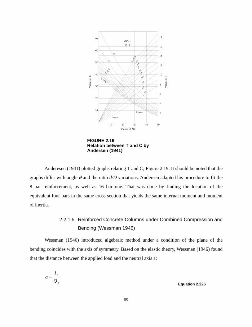
59
70
60
50
40
30
20
10
10 20 30 40 50
Val
ues
of C
Values of D/e
Val
ues
of T
d/D=.1 0
c curves
T curves
7018
16
14
12
10
8
6
4
2
n p=1
.00.
90.
80.
70.
60.
50.
40.
30.
20.
1
np =1.0
0.1
0.20.3
0.40.5
FIGURE 2.19 Relation between T and C by Andersen (1941)
Anderesen (1941) plotted graphs relating T and C; Figure 2.19. It should be noted that the
graphs differ with angle and the ratio d/D variations. Andersen adapted his procedure to fit the
8 bar reinforcement, as well as 16 bar one. That was done by finding the location of the
equivalent four bars in the same cross section that yields the same internal moment and moment
of inertia.
2.2.1.5 Reinforced Concrete Columns under Combined Compression and
Bending (Wessman 1946)
Wessman (1946) introduced algebraic method under a condition of the plane of the
bending coincides with the axis of symmetry. Based on the elastic theory, Wessman (1946) found
that the distance between the applied load and the neutral axis a:
p
p
Q
Ia
Equation 2.226

60
Ip = moment of inertia of the effective area with respect to the load axis
Qp = the first moment of the effective area.
The procedure proposed has very limited applicability since it required the applied load
lies on the axis of symmetry, which consider a very special case. In addition it relies on the
elastic theory.
2.2.1.6 Analysis of Normal Stresses in Reinforced Concrete Section
under Symmetrical Bending (Bakhoum 1948)
Using the elastic theory and equating the internal forces and moments to the applied one,
Bakhoum (1948) developed procedure in locating the neutral axis. This procedure was set for
uniaxial bending. He also intensified the importance of taking the tensioned concrete into
account while analyzing.
1
1'
s
iH
Equation 2.227
t
HH '
Equation 2.228
3bt
nIi ps
Equation 2.229
2bt
nSs ps
Equation 2.230
H = distance between the load and the neutral axis
N= modular ratio
b= section width
t = section height

61
Ips = Moment of inertia of the total reinforcement steel about the line parallel to the
neutral axis through the point of application of the external force.
Sps = Statical moment of the total reinforcement steel about the line parallel to the neutral
axis through the point of application of the external force.
The relation between and is plotted graphically; Figure 2.20.
0.01
0.02
0.03
0.04
0.05 0.1
0.2
0.3
0.4
0.5
1.0
2.0
3.0
4.0
5.0
10.0
20.0
30.0
40.0
50.0
100.
0Values of 10 1 and 1
-0.5
0.0
0.5
1.0
1.5
2.0
2.5
3.0
3.5
c
P
HC
Z
t
bIpc = bt
Spc = bt
Z' = Z/t
C' = C/t
3
2
1
1
valu
es o
f f
or Z
' = 0
.11
0.2
0.3
0.4
0.5
0.6
0.7
0.8
0.9
1.0 va
lues
of 1
0 fo
r Z' =
0.1
1
0.2
0.3
0.4
0.5
0.6
0.7
0.8
0.9
1.0
FIGURE 2.20 Relation between c and byBakhoum (1948)
For the case of unsymmetrical bending, Bakhoum (1948) suggested three solutions;
methods of center of action of steel and concrete, product of inertia method and method of
mathematical successful trial. It is noted that the first two methods are trial and error methods,
and all the three methods were built on the elastic linear theory.

62
2.2.1.7 Design of Rectangular Tied Columns Subjected to Bending with
Steel in All Faces (Cervin 1948)
The Portland cement association published “continuity in concrete frames” (third edition)
that has an equation that relates the maximum load to the actual applied load and moment. It can
be applied on a cross section:
t
MCDNP
Equation 2.231
P = total allowable axial load on column section
N= actual axial load on column section
M = moment
T = section height
'45.0 c
a
f
fC
Equation 2.232
fa = the average allowable stress on axially loaded reinforced concrete column
2
2
2R
tD
Equation 2.233
R = radius of gyration
This equation is limited to reinforcement on the end faces. Crevin (1948) redefined the
term D in the equation to fit reinforcement in the four faces as follow
22 1167.0
11
pgnyzx
pnD
Equation 2.234
c
s
E
En
Equation 2.235

63
p = reinforcement ratio
g = ratio between extremities of column steel and overall column depth
x = ratio of total column steel at one end
y = ratio of total column steel between centroid and one end
z = arm from cetroid of steel ratio y to centroid of column
t gt
gt2 Z
y
X
CENTROID OF COLUMN
b
FIGURE 2.21 Geometric Dimensions in Crevin Analysis (1948)
He showed that x+yz2 vary from 0.25 to 0.5. The limitation of this equation applicability
is that the ratio e/t has to be less than one.
2.2.1.8 The Strength of Reinforced Concrete Members Subjected to
Compression and Unsymmetrical Bending (Mikhalkin 1952)
Mikhalkin (1952) performed studies on determination of the allowable load and ultimate
load of biaxially loaded rectangular members. He developed design and analysis procedure for
tension and compression failure according to ultimate theory, as he generated charts for design
simplification based on the elastic theory using simple compatibility equations Figure 2.22 and
2.23. These charts locate the concrete and steel centers of pressure with respect to the neutral
axis.

64
0 0.1 0.2 0.3 0.4 0.50
0.2
0.4
0.6
0.8
1.0
1.2
1.4
1.6
1.8
2.0
2.2
2.4
2.6
2.8
3.0
Xc/b or Yc/h
K=2
0<K<1
K=3
J
3.2
3.4
FIGURE 2.22 Concrete Center of Pressure versus Neutral Axis Location, Mikhalkin 1952
-2 -1 0 1 2 3 4 5 6 70
1
2
3
4
5
k=2
k=1
k=0.75
k=2
k=1
k=0.75
k=2
k=0.
5
R=
j
X 1/b1 or Y 2/h1
J
FIGURE 2.23 Steel Center of Pressure versus Neutral Axis Location, Mikhalkin 1952

65
2.2.1.9 Eccentric Bending in Two Directions of Rectangular Concrete
Columns (Hu 1955)
Hu (1955) followed the elastic assumption in building his analysis. He showed
numerically that the slope of the neutral axis for non homogeneous section can be replaced by
that of homogeneous one with small error percentage. He found algebraically the equilibrium
equations
1
2
1
2
1
6 khnp
chk
bdf
N
c Equation 2.236
k
a
h
anff yx
cs
111
Equation 2.237
k
Qnpccm
chkme
bdf
Ndby
c 122
1
2
1
61 2
Equation 2.238
npnqnqmQ yx 2
Equation 2.239
N = the normal compressive force
b = section width
d = section height
fc = maximum concrete strength
h and k define the position of the neutral axis
c, cb, cd coefficients (functions of h)
Ax = cover in x direction coefficient
Ab = cover in y direction coefficient
ex = load eccentricity from the geometric centroid (in x-direction)
ey= load eccentricity from the geometric centroid (in y-direction)
c
s
E
En
Equation 2.240

66
c
s
A
Ap
Equation 2.241
cx
sxx I
Iq
cy
syy I
Iq
Equation 2.242
y
x
e
em
Equation 2.243
The previous equations are plotted graphically to obtain the unkown values k, n/bdf’c,
Figure 2.24.
0 0.1 0.2 0.3 0.4 0.5 0.6 0.7 0.8 0.9 1.0 1.1 1.2 1.3 1.4 1.5
0 0.1 0.2 0.3 0.4 0.5 0.6 0.7 0.8 0.9 1.0 1.1 1.2 1.3 1.4 1.5
0.1
0.2
0.3
0.4
0.5
0.6
0.7
0.8
0.9
1.0
1.1
1.2
1.3
1.4
1.5
0.1
0.2
0.3
0.4
0.5
0.6
0.7
0.8
0.9
1.0
1.1
1.2
1.3
1.4
1.5
Value of e y
Value of e x
Val
ue o
f e
y
Value of e
x
Q=3
K=0.3
K=
0.9
0.4
0.5
0.6
0.70.
8
0.80.7
0.6
0.5
0.4
K=0
.3
0.3
0.3
0.2
0.15
0.100.09
0.080.07
0.06
0.05
0.045
0.040
0.038
0.036
0.034
0.032
0.030
0.029
0.028
0.027
0.026
0.025
0.024
0.023
0.022
0.021
=0.020
Nbdf
c
Nbdfc
=0.015Q=1
0.016
0.0170.0180.0190.0200.0210.0220.0230.0240.0250.0260.0270.0280.029
0.0300.0320.0340.036
0.0380.0400.0450.050.06
0.070.080.090.10
0.15
0.2
FIGURE 2.24 Bending with Normal Compressive Force Chart np = 0.03, Hu (1955). In His Paper the Graphs Were Plotted with Different Values of np 0.03,0.1 ,0.3
The first obvious interest in the ultimate strength of the structural members appeared in
the first half of the past century. Prior to that, there were some designations to the importance of
designing with ultimate strength. While Thullies’s flexural theory (1897) and Ritter’s
introduction of the parabolic distribution of concrete stresses (1899) were introduced prior to the

67
straight line theory of Coignet and Tedesco (1900). The straight line theory became accepted due
to its simplicity and the agreement with the tests’ requirements that time. Coignet’s theory grew
widely till it was contradicted by some experimental work done on beams by Lyse, Slatter and
Zipprodt in 1920’s, and on columns by McMillan (1921), as the concrete’s construction
applicability was spreading out (ACI-ASCE committee 327(1956)). After 1950 there was a call
to start working with the ultimate strength design as it was adopted in several countries in Europe
and others, as the reinforced concrete design has advanced. This led the ACI-ASCE committee
327 to propose the first report on ultimate strength design in 1956 (ACI-ASCE committee
327(1956)). The committee members showed in their studies that the ultimate strength design
load can be found accurately.
They defined the maximum load capacity for concentric load
yststgco fAAAfP )(85.0 '
Equation 2.244
gA = the gross area of the section.
stA = steel bars area
The committee considered minimum eccentricity value to design with. For tied columns
the value was 0.1 times the section’s depth.
For combined axial load and bending moment
ssysucu fAfAkbdkfP '1
'85.0 Equation 2.245
d
ddfAkk
k
kkkbdfeP ysuucu
''
11
21
2' 1185.0 Equation 2.246
uP = axial load on the section
e= eccentricity of the axial load measured from the centroid of tensile reinforcement.
sf = stress in the tensile reinforcement.
udk = distance from extreme fiber to neutral axis, where uk is less than one

68
1k = ratio of the average compressive stress to 0.85 'cf , where 1k is not greater than 0.85
and is to be reduced at the rate of 0.5 per 1000 psi for concrete strength over 5000 psi.
2k = ratio of distance between extreme fiber and resultant of compressive stresses to
distance between extreme fiber and the neutral axis.
1
2
k
k should not be taken less than 0.5.
After ultimate strength design was released, the ACI committee 318 in their “Building
code requirements for reinforced concrete (ACI 318-56)” approved the usage of the ultimate
strength method for designing reinforced concrete members along with the standard method in
1956. They conditioned that:
1b
by
b
bz
a
a
F
f
F
f
F
f
Equation 2.247
Given that the ratio e/t does not exceed 2/3 where
byf= the bending moment about y-axis divided by section modulus of the transformed
section relative to y-axis.
bzf = the bending moment about y-axis divided by section modulus of the transformed
section relative to y-axis.
e = eccentricity of the load measured from the geometric centroid
t = overall depth of the column
af = nominal axial unit stress.
bf = allowable bending unit stress = gsc pff '225.0*8.0
gp= steel ratio to the gross area.
sf = nominal allowable stress in reinforcement.
2.2.1.10 Guide for Ultimate Strength Design of Reinforced Concrete
(Whitney and Cohen 1957)
Following this massive change in paradigm, Charles Whitney and Edward Cohen
released their paper “ guide for ultimate strength design of reinforced concrete” which served as

69
a supplement to the ACI building code (318-56). They suggested a linear relationship between
the case of the pure bending and that of concentric load in the following equation
o
uo
o
u
P
PP
M
M
Equation 2.248
Mu = total moment of the plastic centroid of the section.
Po = ultimate direct load capacity for a concentrically loaded short column.
Pu = ultimate direct load capacity for an eccentrically loaded short column.
Mo = the moment capacity without thrust as controlled by compressin assuming enough
tensile steel to develop it in full and it is equal to
''''2333.0 ddfAfbdM ysco
Equation 2.249
They limited the maximum moment allowed for design to Mu using the following
equation
d
dfpf
bd
Myc
u'
'''2
1306.0 Equation 2.250
'' 85.0 cyy fff Equation 2.251
bdAp s /'' Equation 2.252
As’ = compressive steel area.
d = distance from extreme compressive fiber to centroid of tension force in tensile
reinforcement.
d’ = distance from extreme compressive fiber to centroid of tension force in compressive
reinforcement.
b = column width.

70
0 Mu Mo
Pu
Po
Moment, Pu e' LIMITING VALUE OFMOMENT FOR DESIGN
FIGURE 2.25 Linear Relationship between Axial Load and Moment for Compression Failure Whitney and Cohen 1957
2.2.1.11 Ultimate Strength Design of Rectangular Concrete Members
Subjected to Unsymmetrical Bending (Au 1958)
Au (1958) generated charts to calculate the equivalent compressive depth of the stress
block based on assumed values of section’s dimensions and bars arrangements. The design
equations were created complying with the ACI-ASCE assumptions.
He showed that when a member is subjected to compressive force as well as bending, the
section can be controlled either by tension or compression failure depending on the magnitude of
eccentricities.
His procedure is to first approximate the location of the neutral axis that can be made by
observing that the applied load, the resultant of the tensile force in steel and the resultant of the
compressive forces in compressive steel and concrete must all lie in the same plane. This
classifies the problem as one of the three cases:
1. Neutral axis intersects with two opposite sides
2. Neutral axis intersects with two adjacent sides forming a compression zone bigger
than half of the cross sectional area

71
3. Neutral axis intersects with two adjacent sides forming a compression zone
smaller than half of the cross sectional area
Equilibrium equations plus compatibility equations are needed when the section is
controlled by compression (concrete crush). Whereas, equilibrium equations are sufficient in
tension controlled cases. Tung specified two conditions based on ACI-ASCE report, that are the
average stress sf is assigned to each tensioned bar and the resultant tensile force is considered
the tensile bar group centroid. Based on that, the bars close to the neutral axis are ignored in
computations. Having equilibrium equations, Tung denoted six dimensionless variables, two for
each case of the three cases mentioned above and plotted charts relating each two associated
variables Figures 2.26, 2.27, and 2.28. The charts generated have an output of determining the
neutral axis position. The dimensionless variables utilized are:
t
e
t
r
btf
P
t
d
t
dmp
d
tc yy
c
uyy
y
'
'
'''
2
1 85.0 Equation 2.253
b
e
b
r
btf
P
b
d
b
dmp
d
tc xx
c
uxx
y
'
'
'''
2 85.0 Equation 2.254
t
e
t
r
btf
P
t
d
t
dmp
dd
btQ yy
c
uyy
yx
'
'
'''
2
2
1 85.0
2
Equation 2.255
b
e
b
r
btf
P
b
d
b
dmp
dd
tbQ xx
c
uxx
yx
'
'
'''
2
2
2 85.0
2 Equation 2.256
t
e
t
r
btf
P
t
d
t
dmp
t
rU yy
c
uyyy'
'
'''
1 85.0 Equation 2.257
b
e
b
r
btf
P
b
d
b
dmp
b
rU xx
c
uxxx'
'
'''
2 85.0 Equation 2.258

72
e'y
t/2
d'y
r'y
ry
c
dx
b
dy
t
g go
e'xb/2rx r'x d'x
Pu
NA
h
T
Cs
0
0.1
0.2
0.3
0.4
0.5
0.6
0.7
0.8
0 0.1 0.2 0.3 0.4 0.5
g/dy
go/dy
C1=0.45
0.40
0.35
0.30
0.40
0.20
0.15
0.10
0.05
0
0.25
C2=0.11
0.100.09
0.08
0.07
0.06
0.05
0.040.030.02
0.01
a= K h1
FIGURE 2.26 Section and Design Chart for Case 1(rx/b = 0.005), Au (1958)
e'y
t/2
d'y
r'y
ry
dx
b
dy
t
e'xb/2rx r'x d'x
Pu
NA
T
Cs
nxn'x
nyn'y
h
0.1 0.2 0.3 0.4 0.50 0.6 0.7 0.8 0.9 1.0
0.1
0.2
0.3
0.4
0.5
0.6
0.7
0.8
0.9
1.0
Q1/Q2=0.8
0.9
1.0
1.1
1.2
1.31.4
0.7
Q1=0.1
0.2
0.3
0.4
0.5
0.6
nx/d
x
ny/dy
1a=k h
FIGURE 2.27 Section and Design Chart for Case 2, Au (1958)

73
e'y
t/2
d'y
r'y
ry
dx
b
dy
t
e'xb/2rx
r'xd'x
Pu
NA
T
Cs
w'xwx
w'ywy
h
a=k h
0.1 0.2 0.3 0.4 0.50 0.6 0.7 0.8 0.9
0.1
0.2
0.3
0.4
0.5
0.6
0.7
0.8
0.9
Wy/
tWx/b
U1=0.025
0.02
0.015
0.010.005
0.0025
U1/U2=0.2
0.4
0.6
0.8
1
1.5
2.03.0
1
FIGURE 2.28 Section and Design Chart for Case 3(dx/b = 0.7, dy/t = 0. 7), Au (1958)
t = total depth of rectangular section
dy = distance from extreme compressive corner to centroid of tensile reinforcement
measured in the direction of y-axis
p’ = A’s/bt
b = width of rectangular section
m’ = m-1 , m =fy/0.85f’c
d’y = distance from extreme compressive corner to centroid of compressive reinforcement
measured in the direction of y-axis.
Pu = ultimate direct load capacity for the member subject to bending in two directions
ry = distance from centroid of tensile reinforcement to x’-axis.
rx = distance from centroid of tensile reinforcement to y’-axis.
e’y = eccentricity of ultimate direct load measured from centroid of rectangular section in
the direction of y-axis
d’x = distance from extreme compressive corner to centroid of compressive reinforcement
measured in the direction of x-axis
74
dx = distance from extreme compressive corner to centroid of tensile reinforcement
measured in the direction of x-axis
e’x = eccentricity of ultimate direct load measured from centroid of rectangular section in
the direction of x-axis.
2.2.1.12 Design of Symmetrical Columns with Small Eccentricities in One
or Two Directions (Wiesinger 1958)
Using the section moment of inertia and the section modulus, Wiesinger (1957)
introduced a new designing equation for the gross sectional area required by design for columns
subjected to small eccentricities in one direction or two. Wiesinger (1957) proposed gross section
equation:
gsgbgscg pgnF
tNe
pffQ
NA
2
'
' 1
/
225.0
Equation 2.259
and the capacity of a given column is calculated using the following equation
gsgbgsc pgnF
te
pffQ
N
2
'
' 1
/
225.0
1
Equation 2.260
g
gg At
I2
2
Equation 2.261
s
ss
Agt
I2
2
Equation 2.262
Ag = gross area
As= Steel area
t = column length in the direction of bending

75
Ig= gross moment of inertia in the bending direction
Is= moment of inertia of steel in the bending direction
e’ = eccentricity of the resultant load measured to center of gravity
N= applied axial load
Q= reduction factor = 0.8 for short tied column
pg = As/Ag
Fb= allowable bending unit stress that is permitted if bending stress existed = 0.45 f’c
G = center to center steel in the direction of bending divided by column length in the
direction of bending
2.2.1.13 Biaxially Loaded Reinforced Concrete Columns (Chu and
Pabarcius 1958)
In 1958 Chu and Pabarcius introduced a new numerical procedure to determine the actual
stresses for a give section. Their procedure was based on the inelastic theory showed earlier by
Hogenstad. Initially, they assumed the cross section is in the elastic range, and assumed a
location for the neutral axis. Then used the following formula that was found by Hardy Cross
(1930), to solve for stresses
Y
I
II
I
IMM
X
I
II
I
IMM
A
Pf
oy
oxyox
ox
oxyoyox
ox
oxyoy
ox
oxyoxoy
E2
""
2
""
"
Equation 2.263
f = stress
Ae = Area of the elastic portion.
Iox = moment of inertia about x-axis
Ioy = moment of inertia about y axis
Ioxy = product of inertia
M”oy =moment of the elastic portion about the y axis
M”ox =moment of the elastic portion about the x axis

76
P” = axial force taken by the elastic portion.
If the concrete and steel stresses lie in the elastic range, the above equation was used to
locate a new position for the neutral axis, and comparing it with the assumed one. The whole
process is repeated till the position of the calculated neutral axis coincides with the assumed one.
On the other hand if any of the concrete or steel are beyond the elastic range, the plastic load and
moments are calculating, then deducted from the total load and moments. The reminder is used,
as the elastic portion of the load, to locate the neutral axis.
2.2.1.14 Design Criteria for Reinforced Columns under Axial Load and
Biaxial Bending (Bresler 1960)
Bresler (1960) proposed a new approach of approximations of the failure surface in two
different forms. He showed the magnitude of the failure load is a function of primary factors;
column dimensions, steel reinforcement, stress-strain curves and secondary factors; concrete
cover, lateral ties arrangement. He introduced two different methods. The first method named
reciprocal load method
oyxi PPPP
1111
Equation 2.264
Pi =approximation of Pu
Px = load carrying capacity in compression with uniaxial eccentricity x.
Py = load carrying capacity in compression with uniaxial eccentricity y.
Pu = load carrying capacity under pure axial compression
The second method is the load contour
1
yo
y
xo
x
M
M
M
M
Equation 2.265
and this can be simplified to
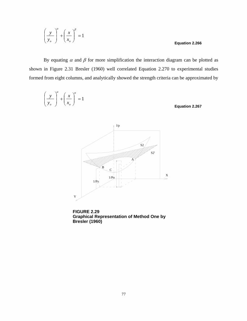
77
1
oo x
x
y
y
Equation 2.266
By equating and for more simplification the interaction diagram can be plotted as
shown in Figure 2.31 Bresler (1960) well correlated Equation 2.270 to experimental studies
formed from eight columns, and analytically showed the strength criteria can be approximated by
1
oo x
x
y
y
Equation 2.267
X
Y
C
S2
A
B
l/p
S2'
1/Po1/Py
FIGURE 2.29 Graphical Representation of Method One by Bresler (1960)

78
My
Mx
Mxo
Myo
Pu
LOAD CONTOUR
PLANE PA CONSTANT
FAILURE SURFACE S3
P M INTERACTION CURVES
P
2 24 .6 84 4
FIGURE 2.30 Graphical Representation of Method Two by Bresler (1960)
X/Xo
1.0
Y/Yo
1.0
0.8
0.6
0.4
0.2
00.80.60.40.20
= 1
= 1.4
= 2
= 3
= 4
FIGURE 2.31 Interaction Curves Generated from Equating and by Bresler (1960)

79
2.2.1.15 Rectangular Concrete Stress Distribution in Ultimate Strength
Design (Mattock and Kritz 1961)
Mattock and Kritz (1961) determined five cases for the position of the neutral axis with
respect to the rectangular cross section; when the neutral axis cut through two adjacent sides with
small and big compression zone, the neutral axis intersect with the section length or width and
when it lies outside the cross section. They implemented formulas for calculating the position of
the neutral axis based on the load and moment equilibrium and the geometry of the compression
zone.
2.2.1.16 Square Columns with Double Eccentricities Solved by
Numerical Methods (Ang 1961)
Ang (1961) introduced a numerical method to solve the problem. He proposed iterative
process to find equilibrium between internal forces and applied ones, by assuming a position for
the neutral axis. The location of the neutral axis kept changing till equilibrium. However, he
calculated stresses based on Bernoulli’s plane theorem which was built upon straight line theory
(elastic theory). The stress of the extreme compression fiber was approximately calculated
according to the specification of AASHTO 1957 “Standard specifications for highway bridges”.
2.2.1.17 Ultimate Strength of Square Columns under Biaxially Eccentric
Load (Furlong 1961)
Furlong (1961) analyzed square columns that have equal reinforcement in the four sides
and reinforcement in two sides only, to visualize the behavior of rectangular columns that has
unsymmetrical bending axis. He used a series of parallel neutral axis with the crushing ultimate
strain of 0.003 at one of the section corners to develop a full interaction diagram at one angle.
And by using different angles and locations of the neutral axis a full 3D interaction surface can
be developed. He was the first to introduce this procedure. Furlong (1961) concluded that the
minimum capacity of a square column, having equal amount of steel in all sides, exists when the
load causes bending about an axis of 45 degree from a major axis. He also concluded that
1
22
y
y
x
x
M
m
M
m
Equation 2.268

80
Mx = moment component in direction of major axis.
My = moment component in direction of minor axis.
Mx = moment capacity when the load acts along the major axis.
My= moment capacity when the load acts along the minor axis.
2.2.1.18 Tie Requirements for Reinforced Concrete Columns (Bresler
and Gilbert 1961)
Bresler (1961) introduced the importance of the tie confinement in columns as objects to
hold the longitudinal bars in place and prevent them from buckling after the cover spalling off.
No concrete strength improvement was discussed.
2.2.1.19 Analytical Approach to Biaxial Eccentricity (Czerniak 1962)
Czerniak (1962) proved that the slope of the neutral axis is depending on the relative
magnitude of moment about the X axis to the moment about the Y axis and the geometry of the
sections and it is independent of the magnitude of bending moment and the applied force for the
elastic range. According to the effective compressive concrete, Czerniak (1962) determined five
cases based on the location of the neutral axis, Figure 2.44.
(a) (b) (c) (d) (e)
FIGURE 2.32 Five Cases for the Compression Zone Based on the Neutral Axis Location Czerniak (1962)
He developed an iterative procedure for locating the neutral axis position for a given
cross section, by using equations 2.272 and 2.273 to determine the initial position of the neutral
axis oxpoxpoyoxpxypox
oypoyoxpoxoxpxyoypxy
QYIAXQQXIAYQ
QXIQYIQXIQYIa
Equation 2.269

81
oypoypoxoypxypox
oypoyoxpoxoxpxyoypxy
QXIAYQQYIAXQ
QXIQYIQXIQYIb
Equation 2.270
a = x-intercept of the neutral axis line
b = y-intercept of the neutral axis line
xyI = elastic product of inertia of the area about the origin
oxI =elastic moment of inertia of the area about the x-axis
oyI =elastic moment of inertia of the area about the y-axis
oxQ = moment area about x-axis (within elastic region)
oyQ = moment area about y-axis (within elastic region)
A = area of transformed section (within elastic regions)
pY = y-coordinate of the applied eccentric load
pX = x-coordinate of the applied eccentric load
then calculating the new section properties, effective concrete and transformed steel, and
finding the new values of Xp and Yp.
b
y
a
x
b
r
a
ry
Y
oxxy
p
1
22
Equation 2.271
b
y
a
x
b
r
a
rx
X
xyoy
p
1
22
Equation 2.272
and solving for a, b again and repeat the procedure up till convergence.
As for ultimate strength design, Czerniak (1962) proved with some simplification that the
neutral axis is parallel to concrete plastic compression line and steel plastic tension and

82
compression line, so they can be found by multiplying the location of the neutral axis by some
values. The ultimate eccentric load and its moment about x and y axis can be found from:
b
Q
a
QAfP oxoy
uou'
Equation 2.273
puoxxy
uxoux YPb
I
a
IQfM
'
Equation 2.274
puxyoy
uyouy XPb
I
a
IQfM
'
Equation 2.275
xsxsxcoxux mQQmQQQ '' )1( Equation 2.276
ysysycoyuy mQQmQQQ '' )1( Equation 2.277
of = stress intensity at the origin
and the x-axis and y-axis intercept of the neutral axis are found:
oxpoxupuyoxpxyupux
oypoyoxpoxoxpxyoypxy
QYIAXQPXIAYQ
QXIQYIQXIQYIa
''''
Equation 2.278
oypoyupuxoypxyupuy
oypoyoxpoxoxpxyoypxy
QXIAYQQYIAXQ
QXIQYIQXIQYIb
'''
Equation 2.279
where
ususuco
cu mAAmA
f
fAA '
"' 1
Equation 2.280

83
xsxsxco
coxux mQQmQ
f
fQQ '
''' 1
Equation 2.281
ysysyco
coyuy mQQmQ
f
fQQ '
''' 1
Equation 2.282
xcQ = moment of area about x-axis of the plastic portion of the concrete effective section
ycQ = moment of area about y-axis of the plastic portion of the concrete effective section
xsQ = moment of area about x-axis of the plastic portion of the yielded tensile
reinforcement
ysQ = moment of area about y-axis of the plastic portion of the yielded tensile
reinforcement 'xsQ = moment of area about x-axis of the plastic portion of the yielded compressive
reinforcement 'ysQ = moment of area about y-axis of the plastic portion of the yielded compressive
reinforcement 'uA = equivalent plastic transformed area.
ucA = area of concrete under plastic compression
usA = area of yielded tensile reinforcement 'usA = area of yielded compressive reinforcement.
uP = ultimate strength of eccentrically loaded cross section
uxM = moment of the ultimate load about x-Axis
uyM = moment of the ultimate load about y-Axis
''cf = maximum concrete stress at ultimate loads (assumed as 0.85 f’c)
"c
y
f
fm

84
2.2.1.20 Failure Surfaces for Members in Compression and Biaxial
Bending (Pannell 1963)
Pannell implemented a relation between the failure moment about y-axis for a given load
and the y component of radial moment with the same load. The formula was found based on
deviation study between the actual load contour curve and an imaginary curve found from the
revolution of the failure point about y axis, with the same load, about the z axis. The equation
found for sections that have equal steel in each face:
2sin1 2N
MM y
fy
Equation 2.283
fy
d
M
MN 1
Equation 2.284
Mfy = failure moment for some load in plane y
= angle between y and the transformed failure plane
He showed that his formula is more accurate and conservative than that of Bresler. He
also developed a chart for N for unequal steel distribution; Figure 2.33.
P/f'cbd
fy/f
'c
FIGURE 2.33 Values for N for Unequal Steel Distribution by Pannell (1963)

85
2.2.1.21 Ultimate Strength of Column with Biaxially Eccentric Load
(Meek 1963)
Meek (1963) assumed constant ratio of moment about the x-axis and the y-axis.
Consequently, increasing the force will increase the moment proportionally.
.conste
e
M
M
y
x
x
y Equation 2.285
Using the above relation a location of the neutral axis is selected. Then this location is
adjusted until the following relation is satisfied
ststscscccu fAfAfAP Equation 2.286
He also showed set of experimental points correlated well to the theoritical interaction
diagram developed.
2.2.1.22 Biaxial Eccentricities in Ultimate Load Design (Aas-Jakobsen
1964)
To comply with local design code, Aas-jakbosen (1964) replaced biaxially eccentric load
acts on a regtangular cross section with an equivelant load acts on the main axis of symmetry
with an equivelant moment. He showed , using moment and force equilibrium, that the eqivelant
moment Me:
mcMPeM xe 1
Equation 2.287
yx
xy
te
tec
Equation 2.288
21 cm Equation 2.289

86
The moment M1 is small additional moment depends on failure mode and some other
factors. And in most cases it is equal to zero.
2.2.1.23 Design of Columns Subjected to Biaxial Bending (Fleming and
Werner 1965)
Fleming and Werner (1965) utilized the formulas found by Mattock (1961) for locating
the neutral axis in the different cases of the compression zone shape along with Furlong (1961)
method, by varying the location and inclination angle of the neutral axis, to plot the interaction
diagram. Fleming and Werner (1965) plotted dimensionless interaction diagram for a square
cross section for fourteen cases using parameters that is commonly used.
Pfy/f'c = 0.80fy = 30000 psi
0.80
1.0
1.5
2.0
3.0
5.0
10.0
Pu/f'cb 2=0.4
0.5
0.6
0.70.80.91.01.11.21.3
1.51.4
0.600.40
ex/ey =0.20
0
0.1
0.2
0.3
0.4
0.5
0.6
0.7
0.1 0.2 0.3 0.4 0.5 0.6 0.7 0.8 0.9
FIGURE 2.34 Design Curve by Fleming et al. (1961)
2.2.1.24 Investigation of the Ultimate Strength of Square and Rectangular
Column under Biaxially Eccentric Loads (Ramamurthy 1966)
Ramamurthy (1966) proposed a new method for defining the load contour for sections
having eight or more bars distributed evenly. He mentioned that the available methods of design
of biaxially loaded column are trial and error procedure and determination of ultimate load from
failure surface. He showed that columns containing four bars behave differently than those
containing eight or more bars with the same reinforcement ratio. He found theoretically for
square columns that the neutral axis inclination angle and the angle formed between the load ray
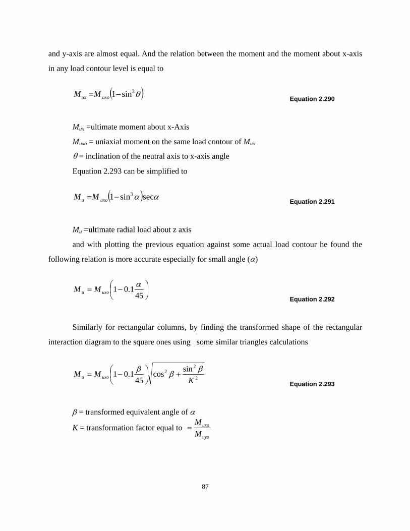
87
and y-axis are almost equal. And the relation between the moment and the moment about x-axis
in any load contour level is equal to
3sin1 uxoux MM
Equation 2.290
Mux =ultimate moment about x-Axis
Muxo = uniaxial moment on the same load contour of Mux
= inclination of the neutral axis to x-axis angle
Equation 2.293 can be simplified to
secsin1 3 uxou MM
Equation 2.291
Mu =ultimate radial load about z axis
and with plotting the previous equation against some actual load contour he found the
following relation is more accurate especially for small angle ()
451.01
uxou MM Equation 2.292
Similarly for rectangular columns, by finding the transformed shape of the rectangular
interaction diagram to the square ones using some similar triangles calculations
2
22 sin
cos45
1.01K
MM uxou
Equation 2.293
= transformed equivalent angle of
K = transformation factor equal to uyo
uxo
M
M

88
Also he showed that the upper equation is in good comparison with experimental actual
load contour. He plotted the relation between and for different ratios of length to width for
rectangular columns.
d/b =
1.0
d/b =
1.5
d/b =
2.0
FIGURE 2.35 Relation between and by Ramamurthy (1966)
2.2.1.25 Capacity of Reinforced Rectangular Columns Subjected to
Biaxial Bending (Parme, Nieves, and Gouwens 1966)
Parme et.al (1966). suggested relating the biaxial bending to the uniaxial resistance. They
restated Bresler equation
1log
5.0log
log
5.0log
uy
y
ux
x
M
M
M
M
Equation 2.294
Mx = uniaxial ultimate moment capacity about x-axis
Muy = uniaxial ultimate moment capacity about y-axis
Mx= biaxial bending capacity component about x-axis.
My= biaxial bending capacity component about y-axis.

89
is a function of reinforcement position, column dimension and the materialistic
properties of steel and concrete. Parme et.al (1966) used a computer program to obtain values for
. Then was represented graphically in four charts, Figure 2.37, 2.38, 2.39, 2.40.
Mx/Mux
My/
Muy
1.0
.9
.9.8.7.6.5.4.3.2.10
1.0
.8
.7
.6
.5
.4
.3
.2
.1
Uniaxial Bending Capacity about x axis = Mux about y axis = MuyBiaxial Bending Capacity about x axis = Mx about y axis = My
= .90
= .50
.85.80
.75.70
.65.60
.55
FIGURE 2.36 Biaxial Moment Relationship by Parme et al. (1966)
0 .1 .2 .3 .4 .5 .6 .7 .8 .9 0 .1 .2 .3 .4 .5 .6 .7 .8 .9
.6<g<1.0
3,000<fc'<6,0001.0<t/b<4.0q = Pt fy/fc'
Pt = Ast / tb
fy = 60,000 psi
.6
.7
.8
1.0
.9
.5
fy = 60,000 psi
q = .1
.3
.5
.9
1.3
Pu/Po Pu/Po
q = .1
.3
.5
.9
1.3
tX
gb
b
Y X
Y
FIGURE 2.37 Biaxial Bending Design Constant (Four Bars Arrangement) by Parme et al. (1966)

90
.6<g<1.03,000<fc'<6,000
1.0<t/b<4.0q = Pt fy/fc'
Pt = Ast / tb
tX
gb
b
Y X
Y
fy = 60,000 psify = 40,000 psi
Pu/Po Pu/Po
q = .1
.3.5
.9
1.3
.3.5
.9
1.3
q = .1
0 .1
.6
.7
.8
1.0
.9
.5
.2 .3 .4 .5 .6 .7 .8 .9 .0 .1 .2 .3 .4 .5 .6 .7 .8 .9
q =1.3
q = .1
FIGURE 2.38 Biaxial Bending Design Constant (Eight Bars Arrangement) by Parme et al. (1966)
.6<g<1.03,000<fc'<6,000
1.0<t/b<4.0q = Pt fy/fc'
Pt = Ast / tb
tX
gb
b
Y X
Y
fy = 60,000 psify = 40,000 psi
.6
.7
.8
1.0
.9
.5
Pu/Po Pu/Po
0 .1 .2 .3 .4 .5 .6 .7 .8 .9 .0 .1 .2 .3 .4 .5 .6 .7 .8 .9
q = .1
.3.5
.9
1.3
q = .1
.3
.5
.9
1.3
q = .1
q = 1.3
FIGURE 2.39 Biaxial Bending Design Constant (Twelve Bars Arrangement) by Parme et al. (1966)

91
.6<g<1.03,000<fc'<6,000
1.0<t/b<4.0q = Pt fy/fc'
Pt = Ast / tb
tX
gb
b
Y X
Y1.0
.9
fy = 60,000 psify = 40,000 psi
.6
.7
.8
.5.1 .2 .3 .4 .5 .6 .7 .8 .9 .0 .1 .2 .3 .4 .5 .6 .7 .8 .9
q = .1
.3
.5
.9
1.3
q = .1
q = 1.3 q = .1
.3
.5
.9
1.3
Pu/Po Pu/Po FIGURE 2.40 Biaxial Bending Design Constant (6-8-10 Bars Arrangement) by Parme et al. (1966)
Parme et al. (1966) showed agreement between the suggested Equation 2.297 and the
theoretical one calculated with equilibrium equations. Furthermore, they simplified the
exponential representation of the upper equation by introducing two equations for two straight
line starting from My/Muy =1 and Mx/ Mux =1 intersecting at the point of equal relative
moment Figure 2.41. The equations of the two straight lines are as follow:
uyux
uyxy M
M
MMM
1
Equation 2.295
ux
uy
uxyx M
M
MMM
1
Equation 2.296

92
Mx/My0
45M
y/M
uy
(Mx/Mux)(1-B/B)+My/Muy = 1
exponential contour
1.0
(Mx/Mux)(My.Muy)+(1-B/B) = 1
FIGURE 2.41 Simplified Interaction Curve by Parme et al. (1966)
2.2.1.26 Ultimate Strength Design Charts for Columns with Biaxial
Bending (Weber1966)
Based on Furlong conclusion that the most critical bending axes is the 45 degree ones
after the major and minor axes in the case of biaxial bending. Weber (1966) generated sixteen
chart for the 45 degree interaction diagrams for square columns. the columns are having
symmetrical reinforcement with different amount of steel bars. Design aids in the 1970 ACI SP-
17A Handbookl2 and the 1972 CRSI Handbookl3 were based on interaction diagrams developed
be Weber (1966).
2.2.1.27 Working Stress Column Design Using Interaction Diagrams
(Mylonas 1967)
Mylonas (1967) adapted the interaction diagrams charts generated in the ACI Design
handbook (1965), that were mainly for columns subjected to axial load and uniaxial bending and
the steel is distributed on two faces parallel to the bending axis, to fit cases of biaxial bending
and steel distributed along the four faces. Two reduction factors were introduced , one for each
zone (Figure 2.42).

93
Region 2
Region 3
Region 1
o
P'bx
N'
N'
P'a
F'a
kox.M'ox M'ox
M'xx
M'bx
r'x.M'xx
rx.M'bx
rx.M'bx M'bx
rx.M'axM'ax
Dx
D'xCompression control zone
Tension control zone
M'x
FIGURE 2.42 Working Stress Interaction Diagram for Bending about X-Axis by Mylonas (1967)
for zone 2:
x
xxx w
wkr
1
1
Equation 2.297
kx is the moment of the steel distributed on two faces and is equal to
2
2
5.0s
xsx
a
ak
Equation 2.298
gxx pgnw 2123 Equation 2.299
gx =bars center
pg = steel ratio
as = section area of arbitrary bar
x = bar distance from x-axis divided by gx t(section height)

94
For zone 3
oxxbx
oxx krP
Nkr
'
''
Equation 2.300
Kox is the moment reduction factor for pure bending about x-axis
5.0s
xsox a
ak
Equation 2.301
P’bx = load at balance failure
N’ = normalized axial load
Mylonas (1967) also suggested that the applied bending moment should be compared to
the reduced moment capacity, the moment capacity found from uniaxial bending interaction
chart, of the section in form
1'
'
'
'
yyy
y
xxx
x
Mr
M
Mr
M
Equation 2.302
M’x ,M’y are the applied moment
M’xx ,M’yy moment capacity
2.2.1.28 Comparison of Experimental Results with Ultimate Strength
Theory for Reinforced Concrete Columns in Biaxial Bending
(Brettle and Taylor 1968)
Brettle and Taylor (1968) suggested partitioning the cross section into small size area,
and using the limiting strain and the neutral axis position in calculating stresses in each filament
using curvilinear stress distribution or rectangular stress distribution or trapezoidal stress

95
distribution for concrete. They generated ultimate strength design charts relating Pu/Po to er/b for
different t/b ratios and different inclination angle beween the line conecting the load to the
centroid and the x-axis.
0 0.2 0.4 0.6 0.8 1.0 1.2 1.4
e / br
0.2
0.1
0.3
0.4
0.5
0.6
0.7
0.8
1.0
0.9b
0.8 b
0.8 tt
Pu/Po
e r
+Pu
= 30
q = 1.0
f sy = 30000 psi
f sy = 75000 psi
t =2b
t = b
t = b
t =2b
FIGURE 2.43 Comparison of Steel Stress Variation for Biaxial Vending When = 30 and q = 1.0
Brettle and Taylor (1968)
er = resultant eccentricityed
t = section height
b = section width
Po = theoretical ultimate load with no eccentricities
Pu= theoretical ultimate load with eccentricities
2.2.1.29 Biaxial Flexure and Axial Load Interaction in Short Rectangular
Reinforced Concrete Columns (Row and Paulay 1973)
Row and Paulay (1974) introduced six charts relating the m to Pu/f’cbh to facilitate the
design process. However these charts are applicable to limited cases only based on the material
properties required for design

96
2'
21
bhf
kMm
c
ux Equation 2.303
x
y
M
Mk Equation 2.304
2.2.1.30 Biaxial Bending Simplified (Gouwens 1975)
Gouwens (1975) proposed simplified analytical equations for design column subjected to
biaxial bending. He utilized Parme et al. (1966) simplified moment Equations 2.298 and 2.299.
He found that approaches 1 for 0.25 f’c bh by examining 67 column cases. Based on that he
proposed equations as follow:
For P ≥ 0.25 Cc
cs
c
CC
CP
85.0
25.02.025 Equation 2.305
For P < 0.25 Cc
csc
CCCP 285.025.02.0
2
25
Equation 2.306
bhfC cc' yss fAC Equation 2.307
s
c
C
C03.0485.025 5.0
s
c
C
C Equation 2.308
2
25 5.035.0545.0
s
c
C
C 5.0
s
c
C
C Equation 2.309

97
2.2.1.31 Analysis of Short Rectangular Reinforced Concrete Columns
Subjected to Biaxial Moments (Sallah 1983)
Sallah (1983) evaluated the Parameter , found by Parme et al. (1966) and found that it
was most affected by fy, f ’c , r, Pu/Puo and less affected by the number of bars. Sallah (1983)
introduced number of charts similar to Parme et al.’s (1966) for finding
2.2.1.32 Design Contour Charts for Biaxial Bending of Rectangular
Reinforced Concrete Columns Using Bresler Method (Taylor
and Ho 1984)
Taylor and Ho (1984) developed a computer program to generate the two main
interaction diagrams (with uniaxial bending-one for each axis). These two charts were used to
generate the whole biaxial failure surface (and the failure contours)using Bresler equations.
Different positions of parallel neutral axis and crushing strain of concrete were used to generate
strain profile. The stresses were generated by stress block or other accepted formulas. And forces
and moments were calculated. They plotted chart showing the load tracing on the cross section.
0 .2 .4 .6 .8 1.0 1.2
.2
.4
.6
.8
1.0
1.2
0.4columnSection
Pn/Po= 0.2
Pn/Po= 0.2
Pn/Po= 0.1
e /tx
e /b y
FIGURE 2.44 Non Dimensional Biaxial Contour on Quarter Column by Taylor and Ho (1984)

98
2.2.1.33 Radial Contour Method of Biaxial Short Column Design (Hartley
1985)
Hartley (1985) proposed two design procedure, one for finding the cross sectional length
and the other to calculate the steel reinforcement, given all other desin parametes. He showed an
optimum point to exist on the 3 D. interaction diagram that relates to the smallest area of the
cross section. Initially, he showed the relation between the load and eccentricity in the form:
b
eC
P
P
o
uln Equation 2.310
where c is a curve constant,b is section length and e is force eccentricity the initial value of the
cross section length can be found by
0*/
ln26.358.3 2
u
x
go
u
P
Mcb
t
b
AP
Pb
Equation 2.311
Hartley (1985), using computer program, plotted graphically the relation between the
cross sectional area and the ratio of Pu/Po. These charts can be used to determine the suitable
length in design.
Pu/Puo
A
fy = 300MPaf'c = 20MPa= 300MPa >= 0.6b/t >= 1
1.0
R
1.0
My/Moy
Mx/Mox
FIGURE 2.45 Pu/Puo to A Relation for 4bars Arrangement by Hartley (1985) (left) Non-Dimensional Load Contour (Right)

99
Hartley (1985) also showed the relation between the R and in the load contour by
2sin1 nAR Equation 2.312
where R and are showen in Figure 2.45 (right).
2.2.1.34 Expert Interactive Design of R/C Columns under Biaxial
Bending (Sacks snd Buyukozturk 1986)
Sacks and Buyukozturk (1986) developed computer software EIDOCC (Expert
interactive design of concrete columns) to analyse and design columns subjected to biaxial
bending. The procedure as follow
1. Finding the neutral axis location, according to Ramamurthy procedure, such that
x
y
ux
uy
e
e
e
etantan
Equation 2.313
eux = ultimate eccentricity measured parallel to x-axis
euy = ultimate eccentricity measured parallel to y-axis
ex = eccentricity measured parallel to x-axis
ey = eccentricity measured parallel to y-axis
2. Using the neutral axis depth,c, for the balanced failure as initial value
3. Calculating Pu and iterating for c using modified secant numerical method till the
load is very close to Pu
4. Calculating euy, eux and comparing them to ey, ex to check section adequacy.

100
2.2.1.35 Interactive Design of Reinforced Concrete Columns with Biaxial
Bending (Ross and Yen 1986)
Ross and Yen (1986) developed a computer program to analyze and design rectangular
columns subjected to biaxial bending. The procedure is to change the inclination angle of the
neutral axis to find adequate relation between Mnx, Mny, and then change the position of the
neutral axis to solve for the axial load. The section capacity is calculated using a predifined
postion of the neutral axis and crushing strain equal to 0.003 for concrete. They suggested using
four bars initially in the design process and keep increasing according to the applied loads with
limiting the number of bars as stated by ACI code.
2.2.1.36 Design of Columns Subjected to Biaxial Bending (Horowitz
1989)
Horowitz (1989) developed a computer program for columns with any cross section
subjected to biaxial bending. He relied on finding the least possible location of steel bars that
make the section capacity more than the applied load.
2.2.1.37 Strength of Reinforced Concrete Column in Biaxial Bending
(Amirthandan 1991)
Amirthandan et.al (1991) showed good corelation between the experimental work done
before and the method propsed in the austrailian standard for concrete structures AS 3600 for
short columns. The load contour in the standard is approximated by bresler equation. They
adopted the beta value from the British standard
NuoN 6.0/7.17.0 Equation 2.314
N = design axial force
Nuo = ultimate axial load.

101
2.2.1.38 Computer Analysis of Reinforced Concrete Sections under
Biaxial Bending and Longitudinal Load (Zak 1993)
Zak (1993) proposed solving the equilibrium equation with the modification of the
secant modulus method. The ultimate strain was not determined. However, it was found using
maximization method.
2.2.1.39 Analysis and Design of Square and Rectangular Column by
Equation of Failure Surface Hsu (1994)
Hsu (1994) proposed equation that covers columns subjected to biaxial bending and axial
compression or tension. The proposed equation is as follow:
0.1
5.15.1
nby
ny
nbx
nx
nbo
nbn
M
M
M
M
PP
PP
Equation 2.315
Pn = nominal axial compression or tension
Mnx, Mny= nominal bending moments about x and y axis
Po = maximum nominal axial compression or axial tension
Pnb = nominal axial compression at balanced strain condition
Mnbx, Mnby = nominal bending moments about x and y axis at balanced strain
condition.
2.2.1.40 Biaxial Interaction Diagrams for Short RC Columns of Any
Cross Section (Rodriguez and Ochoa 1999)
Rodriguez and Ochoa (1999) proposed a general method for analyzing any cross section
subjected to biaxial bending. They developed closed form solution for nominal total axial force
strength and nominal bending moment strengths about the global X and Y-axes. Quasi-Newton’s
method was used to solve these coupled nonlinear equations to locate the neutral axis position.

102
si
n
ibisi
n
ibi
m
icin fAfAPP
bc
111 Equation 2.316
bici
n
ibibisi
n
ibi
n
icia
n
icix
n
iciynx YfAYfAPYMMM
bctttt
11111
cossin Equation 2.317
bici
n
ibibisi
n
ibi
n
icia
n
icix
n
iciyny XfAXfAPXMMM
bctttt
11111
sincos
Equation 2.318
Pn= Nominal axial force strength.
Mnx = nominal bending moment strength about x axis
Mny = nominal bending moment strength about x axis
Xa, Ya = coordinates of origin with respect to global x, xaxes
= angle of inclination of neutral axis with respect to Xaxis;
n = number of reinforcement bars;
nbc = number of rebars located on compression side of cross section;
nt = number of trapezoids used to approximate concrete under compression;
Abi = area of steel rebar i;
fci = concrete stress at reinforcement bar i
fsi = steel stress at reinforcement bar i
Pci = force for each trapazoid.
Mciy = Moment of each trapazoid about y axis.
Mcix = Moment of each trapazoid about x axis.
2.2.1.41 Short Reinforced Concrete Column Capacity under Biaxial
Bending and Axial Load (Hong 2000)
Hong (2000) did not assume any crushing strain limit. He proposed two equation from
equating forces and moments:

103
0e - P
M xL
n
y Equation 2.319
0e - P
M yL
n
x Equation 2.320
where exl , eyl is the load eccentricity to x and y axes respectively.The two equations has three
unknows; the curvature, neutral axis inclination angle and the neutral axis intercipt with the y-
axis. Hong (2000) used the sequential quadratic programming method to solve the case as a
nonlinearly constrained optimization problem.
2.2.1.42 Reliability of Reinforced Concrete Columns under Axial Load
and Biaxial Bending (Wang and Hong 2002)
Wang and Hong (2002) evaluated the parameter (Parme et al. 1966) and fount that it is
insensitive to the reinforced ratio, it is more sensitive to biaxial bending than uniaxial bending, it
increases withload and concncrete compressive strength.
2.2.1.43 Analysis and Design of Concrete Columns for Biaxial Bending:
Overview (Furlong, Hsu, and Mirza 2004)
Furlong et al. (2004) reviewed many of the proposed formulas for analysis. These
formulas were compared to experimental work. They concluded that the equations of Bresler
(1960), although simple, are not very conservative, while Hsu equation is much more
conservative. As Hsu equation can be used in biaxial bending and tension as well. However, both
Hsu equation and Bresler reciprocal load equation can not be used in selecting cross section,
unlike Bresler load contour equation.
2.2.1.44 New Method to Evaluate the Biaxial Interaction Exponent for RC
Columns (Bajaj and Mendis 2005)
Bajaj and Mendis (2005) suggested new equations to evaluate the biaxial interaction
exponenet a found by Bresler (1960). The proposed equations are as follow

104
2noy
ny
nox
nx
M
M
M
M
Equation 2.321
log
5.0logK
Equation 2.322
Bajaj and Mendis (2005) benchmarked their equastion by comparing the results with
experimental work done on 8 (150* 150 mm) columns.
2.2.1.45 Analysis of Reinforced Concrete Columns Subjected to Biaxial
Loads (Demagh, Chabil, and Hamzaoui 2005)
Demagh et al. (2005) suggested solving for the three equations of equilibrium to find the
nominal force Pn, the inclination angle of the neutral axis and the depth of the neutral axis b.
The three equation are:
sicisicin AffPP
Equation 2.323
sisicisiciciciynnx yAffPYxMyMePM cossin Equation 2.324
sisicisicicicixnny yAffPXxMyMePM sincos Equation 2.325
where the subscript i refers to a concrete layer or steel bar element.
2.2.1.46 Analytical Approach to Failure Surfaces in Reinforced Concrete
Sections Subjected to Axial Loads and Biaxial Bending (Bonet,
Miguel, Fernandez, and Romero 2006)
Bonet et al. (2006) developed a new method for the surface failure based on numerical
simulation. The numerical simulation was generated using a computer program capable of
analysing moment-curvature diagram for given axial load and moment ratio. The maximum
value was used as a failure point for the given loads. The failure surface is defined by two

105
directrix curves and generatrix curves. The directrix curves are the curve corresponds to zero
axial force and the one corresponds to balance failure.the generatix curves are defined in
Muy/Mux plane, the first curve connects the pure tension axial load to balnce failure load.
Whearas the second curve connects the balnce failure load to the pure compression load. The
equations for the four curves are as follow
Directrix 1
1sin.cos.
2
,1
1
1
,1
1
yd
d
xd
d
M
M
M
M
Equation 2.326
Directrix 2
1sin.cos.
2
,2
2
1
,2
2
yd
d
xd
d
M
M
M
M
Equation 2.327
generatix 1
0*
1
1
22212
1
d
u
utd
utu
ut
ddd
ut
udu
N
N
NN
NN
N
NMM
n
NMM
Equation 2.328
generatix 2
0
1
1
22212
1
d
u
duc
uu
ut
ddd
ut
udu
M
M
NN
NN
N
NMM
n
NMM
Equation 2.329

106
Md1= absolute value of the nominal bending moment of the section in simple flexure
corresponding to angle beta
Md1,x, Md1,y= nominal bending moments of the section in simple flexure for the x and y
axes, respectively.
Md2 = absolute value of the nominal bending moment corresponding to the maximum
bending capacity
of the section for a particular angle
Md2,x, Md2,y = nominal bending moments corresponding to the maximum flexure capacity
of the section for the x and the y axes, respectively.
, =exponents of the directrices.
23.1
15.122.0
= steel reinforcement
Nu = axial load applied
Nuc = the ultimate axial load in pure compression
Nd2 =balance failure load.
95.07.0*8.0lim
NN
NN
uc
uuc Equation 2.330
Nlim = nominal axial compression at the balanced strain condition
2.2.1.47 Biaxial Bending of Concrete Columns: an Analytical Solution
(Cedolin, Cusatis, Eccheli, Roveda 2006)
Cedolin et al. (2006) introduced analytical solution of the failure envelope of rectangular
R/C cross sections subjected to biaxial bending and to an axial force by approximating the
rectangle to equivalent square section. The analysis was for unconfined concrete and the solution
outcome was dimensionless.

107
2.2.1.48 Comparative Study of Analytical and Numerical Algorithms for
Designing Reinforced Concrete Sections under Biaxial Bending
(Bonet, Barros, Romero 2006)
Bonet et al. (2006) introduced analytical and numerical methods for designing circular
and rectangular cross sections subjected to bi-axial bending. The analytical method uses the
heviside function (Barros et al. 2004) to define the failure strain, then integrate the stress based
on that failure. The numerical method breaks the section into multi thick layers parallel to the
nuteral axis. The internal forces are found by numerical integration of each layer using Gausss-
Legendre quadrature (Barros et al. 2004). They concluded that the two method are effeicint for
circular cross section’s analysis and the modified thick layer integration is more efficient for the
rectangular cross section’s analysis.
2.2.1.49 Investigation of Biaxial Bending of Reinforced Concrete
Columns through Fiber Method Modeling (Lejano 2007)
Lejano (2007) expanded the finite element method found by Kaba and Mahin (1984). To
predict the behavior of unconfined rectangular columns subjected to biaxial bending. The
analysis was limited to uniform semmetric square columns. Lejano (2007) utilized Bazant’s
Endochronic theory for concrete and Ciampi model for steel.
2.2.1.50 Variation of Ultimate Concrete Strain at RC Columns Subjected
to Axial Loads with Bi-Directional Eccentricities (Yoo and Shin
2007)
Yoo and Shin (2007) introduced the modified rectangular stress block (MRSB) to account
for non-rectangular compression zone induced by bi-axial bending. They showed experimentally
that the ultimate strain of concrete exposed to bi-directional eccentricities can reach up to 0.0059.
Based on this finding they introduced new equation for the unconfined ultimate strain as follow:
o
ncu P
P
45.0
003.0003.0 45.0
45.0o
n
P
P Equation 2.331

108
o
ncu P
P1
55.0
003.0003.0 45.0 45.0
o
n
P
P Equation 2.332
b
h145.0
tan
0025.0003.0
b
h1tan0 Equation 2.333
90tan90
0025.0003.0
145.0
b
h
90tan 1
b
h Equation 2.334
No definition for was provided.
2.2.1.51 Capacity of Rectangular Cross Sections under Biaxially
Eccentric Loads (Cedolin, Cusatis, Eccheli, Roveda 2008)
Cedolin et al. (2008) utilized the work of Cedolin et al. 2006 to generate more accurate
moment failure contour through creating one extra points on the contour. This point correspond
to the load acting on rectangle diagonlas and was approximated by using equivelant square to
benefit from symmetry. The developed moment contour was used for better evaluating the
parameter found by Bresler (1960).
2.2.1.52 Development of a Computer Program to Design Concrete
Columns for Biaxial Moments and Normal Force (Helgason
2010)
Helgason 2010 developed a computer program using Matlab for designing unconfined
rectangular hollow or solid columns subjected to axial force and bending moment. Helgason
2010 used the predefined strain profile to generate the interaction diagram and the equivelant
stress block equal to 80% of the compression zone depth. The outcome was compared to
Eurocode.

109
2.2.2 Discussion
According to the literature review, there are five different approaches that treated the
columns under axial load and bending moment problem. These ways are summarized as follow:
1. Trial for locating the neutral axis position such as Parker and Scanlon (1941), Ang
(1961) and Czerniak (1962) works.
2. Implementing closed form equations for special cases such as Andersen (1941),
Wiesinger (1958), Cedolin et al. (2006) and Yoo and Shin (2007) works.
3. Generating charts that relate two or more variable to facilitate the design process,
such as Mikhalkin, Au (1958), Fleming and Werner (1965) and Brettle and Taylor
(1968) works.
4. Developing simplified Interaction diagrams by using coefficients for curve
defining. This method was adopted by some researchers like Whitney and Cohen
(1957), Bresler (1960), Furlong (1961), Parme (1966), Mylons (1967), Bonet et
al. (2006).
5. Generating Sets of ready Interaction diagrams to be used directly by designers,
Weber (1966) and others.
There are some conclusions that can be drawn as follow
The finite layer approach is successful in analysis. This approach was
adopted by some authors such as Brettle and Taylor (1968), Bonet et al.
(2006) and Lejano (2007).
The Bresler Method is one of the most well known and successful method
in predicting the unconfined interaction diagrams and load contours. This
method was utilized and refined by many such as Rammamurthy (1966),
Parme et al. (1966), Gouwens (1975), Sallah (1983) Amirthandan (1991),
Wang and Hong (2002) and Bajaj and Mendis (2005). However it is very
conservative for some cases as shown by Furlong et al. (2004) and others.
Software applications on columns spread and became popular in the
beginning of 1980s.Taylor and Ho (1984) developed computer program

110
based on Bresler Method. Sacks and Bugukoztruck (1986) developed their
program based on iterating for neutral axis and load converge. Ross and
Yen (1986) used the predefined strain profile in their software. Horowitz
(1989) incremented the steel bars till the column capacity exceeded the
load applied. This transition in relying on machines for facilitates
calculations. Hence more accurate and precise analysis is needed to define
exactly the unconfined and confined capacity of different sections.
The predefined strain profile is seen to be one of the most effective and
fast procedure foe unconfined analysis. This method was suggested by
Furlong (1961) and utilized by many, such as Ross and Yan (1986).
There is lack of confinement effect analysis on columns capacity.
Nowadays, there is a need in predicting columns extreme events as stated
by some structural codes like AASHTO-LRFD.

111
Chapter 3: Rectangular Columns Subjected to Biaxial Bending and Axial Compression
3.1 Introduction
Rectangular reinforced concrete columns can be subjected to biaxial bending moments
plus axial force. When the load acts directly on one of the cross section bending axes the
problem becomes of uniaxial bending and axial force. However when the load is applied
eccentrically on a point that is not along any of the bending axes the case is generally biaxial
bending and axial force. The biaxial bending case can be found in many structures nowadays.
This case is visited extensively in the literature aside from the confinement effect. The failure
surface of rectangular columns is 3D surface consisted of many adjacent 2D interaction
diagrams. Each of the 2D interaction diagrams represents one angle between the bending
moment about x-axis and the resultant moment. Many simplifications are introduced to justify
the compressive trapezoidal shape of the concrete compression zone, due to the existence of the
two bending axes. Approximations also were presented to depict the 3D failure shape from the
principal interaction diagrams, in the two axes of symmetry. The most effective procedure found
in the literature is the predefined ultimate strain profile that determines a certain position of the
neutral axis and assigns crushing ultimate strain (typically 0.003) in one of the column corners.
With the advance in technology and the enormous speed of computations, analysis is needed to
plot a more accurate failure interaction diagram for both the unconfined and confined cases.
The methodology in this study is based on two different approaches; the adjusted
predefined ultimate strain profile and the moment of area generalization approaches described
below. The two methods are compared to benchmark the moment of area generalization method
that will be used in the actual capacity analysis (Confined analysis). This analysis is compared to
experimental data from the literature.

112
3.2 Unconfined Rectangular Columns Analysis
3.2.1 Formulations
3.2.1.1 Finite Layer Approach (Fiber Method)
The column cross section is divided into finite small-area filaments (Figure 3.1a). The
force and moment of each filament is calculated and stored. The rebars are treated as discrete
objects in their actual locations. The advantage of that is to avoid inaccuracy generated from
using the approximation of the stress block method, as a representative of the compression zone
and to well treat cases that have compressive trapezoidal or triangular shapes generated from the
neutral axis inclination (Figure 3.1b).
Mx
My
FIGURE 3.1 a) Using Finite Filaments in Analysis b)Trapezoidal Shape of Compression Zone
3.2.1.2 Concrete Model
Concrete is analyzed using the model proposed by Hognestad that was adopted from
Ritter’s Parabola 1899 (Hognestad 1951). Hognestad model is used extensively in numerous
papers as it well explains concrete stress-strain behavior in compression. In addition, it was
utilized by widely used concrete models such as Kent and Park model (1971). The stress-strain
model is expressed using the following equation (Figure 3.2):
a) b)

113
2
' 2o
c
o
ccc ff
Equation 3.1
cf = stress in concrete in compression. '
cf = maximum compressive strength of the concrete.
c = strain at cf
o = strain at 'cf
As shown in Figure 3.2a concrete carries tension up to cracking strength, then it is
neglected in calculation beyond that.
f'c
0.75f'c
Axial strainfk
Axi
al s
tres
s
Axial strain
Axi
al s
tres
s
fy
fy
FIGURE 3.2 a) Stress-Strain Model for Concrete by Hognestad b) Steel Stress-Strain Model
3.2.1.3 Steel Model
Steel is assumed to be elastic up to the yield stress then perfectly plastic as shown in
Figure 3.2b. It is assumed that there is perfect bond between the longitudinal steel bars and the
concrete. According to Bernoulli’s Hypothesis, strains along the depth of the column are
assumed to be distributed linearly.
a) b)

114
3.2.2 Analysis Approaches
The process of generalization of the moment-force interaction diagram is developed
using two different approaches; the adjusted predefined ultimate strain profile and the
generalized moment of area methods. The common features of the two approaches are described
as follow:
3.2.2.1 Approach One: Adjusted Predefined Ultimate Strain Profile
The first approach is the well known method that was used by many researchers and
practicing engineers. The procedure is to assign compressive failure strain at one of the column
corners (0.003) and to vary the position and the inclination angle of the neutral axis that ranges
from zero degree, parallel to the width of the column, to ninety degrees parallel to the height as
shown in Figure 3.3.
0.003
FIGURE 3.3 Different Strain Profiles Due to Different Neutral Axis Positions
Each set of the parallel neutral axes of a certain orientation represents approximately one
2D interaction diagram, and all of the sets from zero to ninety degrees represent the 3D failure
surface in one quadrant, which is identical to the other three quadrants due to the existence of

115
two axis of symmetry with respect of concrete and steel. The procedure is described in the
following steps:
1. Defining the strain profile for each neutral axis position and corner ultimate strain
applied.
2. Calculating strain and the corresponding stress in each filament of concrete and
doing the same for each steel bar Figure 3.4.
0.003
N.A
FIGURE 3.4 Defining Strain for Concrete Filaments and Steel Rebars from Strain Profile
3. Calculating the force and the moment about the geometric centroid for each
filament and steel bar Figure 3.5.
for concrete: for steel
iicici twfP sisisi AfP
Equation 3.2
iYPMx cici _* siYPMx sisi _* Equation 3.3
iXPMy cici _* siXPMy sisi _* Equation 3.4

116
Yi
BXi
wt
Ysi
H
BXsi
Y_si
X_Si
HY_i
X_i 0.003 0.003
FIGURE 3.5 Filaments and Steel Rebars Geometric Properties with Respect to Crushing Strain Point and Geometric Centroid
Summing up the forces and moments, from steel bars and concrete filaments, to get the
internal force and moment about x-axis and y-axis. The resultant force and moments represent
one point on the unconfined interaction diagram (Figure 3.6).
Start
Define
Neutral axis
position & orientation
Determine strain
Calculatec,s,f c,f s
Sum up internal forces and moments
Fz,GMox ,GMoy,GMR
profile based on
End
New Point
0.003 at a corner
FIGURE 3.6 Method One Flowchart for the Predefined Ultimate Strain Profile Method

117
The problem arising from this procedure is that the points developed from one set of
parallel neutral axes are close to but not lined up in one plane. However, they are scattered
tightly near that plane (Figure 3.7). To correct for that, an average angle of )/(cos 1Rx MM is
calculated and another run is established by slightly changing the inclination angle of the
neutral axis of the section with respect to the y-axis and iterating till the angle determined for
each point converges to the average angle . The average angle is taken as the average of all
angles obtained for a certain angle orientation of the neutral axis (Figure 3.3 and Figure 3.7).
P
Mx
Plane of the average angle
Point before correction
Point after correction
My
Figure 3.7 2D Interaction Diagram from Approach One Before and After Correction
The iterations mentioned above converge fast in all cases. This approach yields a very
fast computation since it directly evaluates the ultimate unconfined strain profile. However, no
moment curvature or load-strain history response is available with this approach.
3.2.2.2 Approach Two: Generalized Moment of Area Theorem
Moment of Area Theorem
The very general axial stress equation in an unsymmetrical section subjected to axial
force P and biaxial bending Mx and My (Hardy Cross 1930):

118
xIII
IMIMy
III
IMIM
A
P
xyyx
xyxxy
xyyx
xyyyxz 22
Equation 3.5
z = normal stress at any point (a) in cross section
P = applied load.
A = cross sectional area.
xM = bending moment about the geometric x-axis
yM = bending moment about the geometric y-axis
x = distance between the point (a) and y-axis
y = distance between the point (a) and x-axis
xI = moment of inertia about the geometric x-axis
yI = moment of inertia about the geometric y-axis
xyI = product moment of inertia in xy plane
Rewriting Equation 3.5 to determine the strain at any point in the cross section:
xEIEIEI
EIMEIMy
EIEIEI
EIMEIM
EA
P
xyyx
xyxxy
xyyx
xyyyxz 22
Equation 3.6
In case of linear elastic analysis, E in EA or EI expressions is constant (E=Ec). However,
if the section has linear strain but nonlinear stress profile, it will amount to variable E profile (per
layer or filament) in nonlinear analysis. Accordingly, the section parameters must include
i
ii AE , i
ii IE for a more generalized theory (Rasheed and Dinno 1994). Note that the linear
strain profile of the section from Equation 3.6 yields two distinct constant curvatures:
2 xyyyx
x
EIMEIM
Equation 3.7
2 xyxxy
y
EIMEIM
Equation 3.8

119
x = curvature about the x-axis
y = curvature about the y-axis 22xyyx EIEIEI
To prove Equations 3.7 and 3.8 above, invoke the coupled equations of moments about
the actual or current centroid (Bickford 1998).
yxyxxx EIEIM Equation 3.9
yyxxyy EIEIM Equation 3.10
In a matrix form:
y
x
yxy
xyx
y
x
EIEI
EIEI
M
M
Equation 3.11
Inverting Equation 3.11
y
x
xxy
xyy
y
x
M
M
EIEI
EIEI2
1
Equation 3.12
which reproduces Equations 3.7 and 3.8. Rewriting Equation 3.6 in terms of x and y
xyEA
Pyxz
Equation 3.13
Finding z at the actual or current centroid, since x = y = 0.
EA
P= o
Equation 3.14
Finding z at the geometric centroid,

120
xy yxo EA
P=
Equation 3.15
Solving for P at the geometric centroid;
yxo xEAyEAEAP Equation 3.16
But
yEAEAM x
cG YYy
xEAEAM y
cG XXx
YG is the vertical distance to the geometric centroid measured from bottom, XG is the
distance to the geometric centroid measured from the cross section’s left side, Yc is the vertical
distance to the inelastic centroid measured from the bottom and Xc is the horizontal distance to
the inelastic centroid measured from the cross section’s left side (Figure 3.8).
Thus,
yyxxo EAMEAMEAP Equation 3.17
The general formula of the moments about the geometric x-axis and the geometric y-axis
is derived as follows:
when the moment is transferred from the centroid to the geometric centroid (Figure 5.8a)
yPMM xx Equation 3.18
Substituting Equations 3.9 and 3.16 in 3.17 yields:
yEAMyEAMyEAEIEIM yyxxoyxyxxx Equation 3.19

121
yyxyxxxoxx yEAMEIyEAMEIEAMM Equation 3.20
Similarly (Figure 3.8b):
G
Cy
P
Mx
Mx GC
P
MyMy
xyyG
cx
xc
G
FIGURE 3.8 Transferring Moment from Centroid to the Geometric Centroid
xPMM yy Equation 3.21
xEAMxEAMxEAEIEIM yyxxoyyxxyy Equation 3.22
yyyxxxyoyy xEAMEIxEAMEIEAMM Equation 3.23
The terms yEAMEI xx and xEAMEI yy represent the xEI and yEI about the
geometric centroid respectively using the parallel axis theorem. And the terms xEAMEI xxy
and yEAMEI yxy are equal given that: xyEAxEAM x and xyEAyEAM y . Using
Equations 3.16, 3.19, and 3.22 yields the extended generalized moment of area equation:
y
x
o
yxyy
xyxx
yx
y EIEIEAM
EIEIEAM
EAMEAMEA
M
Mx
P
Equation 3.24
a) b)

122
Since the moment of area about the inelastic centroid vanishes (Rasheed and Dinno
1994), Equation 3.23 reduces to a partially uncoupled set when it is applied back at inelastic the
centroid since EAMx and EAMy vanish about that centroid.
y
x
o
yxy
xyx
y
x
EIEI
EIEI
EA
M
M
P
0
0
00
Equation 3.25
which is simply Equations 3.9, 3.10, and 3.14
3.2.2.3 Method Two
This approach simulates the radial loading of the force and moments by keeping the
relative proportion between them constant during the loading. Accordingly, all the points
comprising an interaction diagram of angle will be exactly on that 2D interaction diagram. In
addition to the ultimate points, the complete load deformation response is generated. The cross
section analyzed is loaded incrementally by maintaining a certain eccentricity between the axial
force P and the resultant moment MR. Since MR is generated as the resultant of Mx and My, the
angle = tan-1(My/Mx) is kept constant for a certain 2D interaction diagram. And since increasing
the load and resultant moment proportionally causes the neutral axis to vary unpredictably, the
generalized moment of area theorem is devised. This method is based on the general response of
rectangular unsymmetrical section subjected to biaxial bending and axial compression. The
asymmetry stems from the different behavior of concrete in compression and tension.
The method is developed using incremental iterative analysis algorithm, secant stiffness
approach and proportional or radial loading. It is explained in the following steps. (Figure 3.12
presents a flowchart of the outlined procedure):
1. Calculating the initial section properties:
Elastic axial rigidity EA:

123
Equation 3.26
= initial modulus of elasticity of the concrete
= initial modulus of elasticity of the steel rebar
The depth of the elastic centroid position from the bottom fiber of the section
Yc and from the left side of the section Xc
Equation 3.27
EA
XBAEEXBtwEX i i
sisicsiiic
c
)()()(
Equation 3.28
where Yi and Ysi are measured to the top extreme fiber, Xi and Xsi are measured to the right most
extreme fiber, see Figure 3.9.
Elastic flexural rigidity about the elastic centroid EI:
Equation 3.29
22 )()()( csisici
sciiii
cy XXBAEEXXBtwEEI Equation 3.30
csicsisici
sciciiii
cxy XXBYYHAEEXXBYYHtwEEI )()()(
Equation 3.31
Typically the initial elastic Yc = H/2, Xc = B/2 and EIxy = 0
i
sicsiii
c AEEtwEEA )(
cE
sE
EA
YHAEEYHtwEY i i
sisicsiiic
c
)()()(
22 )()()( csisici
sciiii
cx YYHAEEYYHtwEEI

124
Yi
H
Yc
B
Xc
Xi
wt
C
G
X
Y
G
G
0.003
H
Yc
B
Xc
Xsi
Ysi
X
Y
0.003
0.003 0.003
C
G
G
G
FIGURE 3.9 Geometric Properties of Concrete Filaments and Steel Rebars with Respect to Geometric Centroid and Inelastic Centroid
The depth of the geometric section centroid position from the bottom and left fibers of
the section YG, XG:
Equation 3.32
2
BX G
Equation 3.33
2. Defining the eccentricity e, which specifies the radial path of loading on the
interaction diagram. Also, defining the angle in between the resultant moment
GMR and GMX
2
HYG

125
FIGURE 3.10 Radial Loading Concept
3. Defining the loading step as a small portion of the maximum load, and
computing the axial force at the geometric centroid.
Equation 3.34
4. Calculating the moment GMR about the geometric centroid.
GP
GMe R GPeGM R * Equation 3.35
cosRX GMGM Equation 3.36
tanXY GMGM Equation 3.37
5. Transferring the moments to the inelastic centroid and calculating the new
transferred moments TMX and TMY :
)( cGXX YYGPGMTM
Equation 3.38
e
Resultant MomentA
xial
For
ceLoad Step GP
GP
GPGPGP oldnew

126
)( cGYY XXGPGMTM Equation 3.39
The advantage of transferring the moment to the position of the inelastic centroid is to
eliminate the coupling effect between the force and the two moments, since
0 yx EAMEAM about the inelastic centroid
y
x
o
yxy
xyx
y
x
EIEI
EIEI
EA
TM
TM
P
0
0
00
Equation 3.40
YG
XGXc
Yc
FIGURE 3.11 Moment Transferring from Geometric Centroid to Inelastic Centroid
6. Finding: Curvatures X and Y
XYY
YX
X EITM
EITM
**22
Equation 3.41
XYX
XY
Y EITM
EITM
**22
Equation 3.42

127
22xyYX EIEIEI Equation 3.43
Strain at the inelastic centroid , the extreme compression fiber strain , and strain at
the extreme level of steel in tension are found as follow:
Equation 3.44
)()( cycxoec XBYH Equation 3.45
)()( CoverXCoverY cycxoes Equation 3.46
where cover is up to center of bars
1. Calculating strain and corresponding stress fci in each filament of concrete
section by using Hognestad’s model (Equation 3.1) in case of unconfined analysis
2 2 2 2
y c i y c ix c i x c ici y x xy xy
TM B X X TM H Y YTM H Y Y TM B X XGPEI EI EI EI
EA
Equation 3.47
2. Calculating strain and corresponding stress fsi in each bar in the given section
by using the steel model shown in Figure 3.2b.
2 2 2 2
y c si y c six c si x c sisi y x xy xy
TM B X X TM H Y YTM H Y Y TM B X XGPEI EI EI EI
EA
Equation 3.48
1. Calculating the new section properties: axial rigidity EA, flexural rigidities about
the inelastic centroid EIx,, EIy, EIxy moment of axial rigidity about inelastic
centroid EAMx, EAMy, internal axial force Fz, internal bending moments about the
inelastic centroid Mox ,Moy:
o ec
es
EA
GPo
ci
si

128
i
sicisiiii
ci AEEtwEEA )( Equation 3.49
)()()( sicsicii
siiciii
cix YYHAEEYYHtwEEAM Equation 3.50
)()()( sicsicii
siiciii
ciy XXBAEEXXBtwEEAM Equation 3.51
sicisiiiciz AfftwfF )( Equation 3.52
22 )()()( sicsicii
siiciii
cix YYHAEEYYHtwEEI Equation 3.53
22 )()()( sicsicii
siiciii
ciy XXHAEEXXBtwEEI Equation 3.54
( ) ( ) ( )xy ci i i c i c i si ci si c si c sii i
EI E w t H Y Y B X X E E A H Y Y B X X
Equation 3.55
sicsicii
siiciii
ciox YYHAffYYHtwfM )()( Equation 3.56
sicsicii
siiciii
cioy XXBAffXXBtwfM )()( Equation 3.57
where Eci = secant modulus of elasticity of the concrete filament.
Esi = secant modulus of elasticity of the steel bar.
2. Transferring back the internal moment about the geometric centroid
Equation 3.58
)( cGoyoy XXGPMGM Equation 3.59
)( cGoxox YYGPMGM

129
3. Checking the convergence of the inelastic centroid
Equation 3.60
cyy XEAEAMTOL // Equation 3.61
4. Comparing the internal force to applied force, internal moments to applied
moments, and making sure the moments are calculated about the geometric
centroid :
510*1 zFGP Equation 3.62
510*1 oxx GMGM
510*1 oyy GMGM Equation 3.63
510*1 xTOL 510*1 yTOL
Equation 3.64
If Equations 3.61, 3.62, and 3.63 are not satisfied, the location of the inelastic centroid is
Updated by EAMx/EA and EAMy/EA and steps 5 to 12 are repeated till Equations 3.61, 3.62 and
3.63 are satisfied.
Equation 3.65
EA
EAMXX y
cc oldnew
Equation 3.66
Once equilibrium is reached, the algorithm checks for ultimate strain in concrete and
steel not to exceed 0.003 and 0.05 respectively, then it increases the loading by and
runs the analysis for the new load level using the latest section properties. Otherwise, if
cxx YEAEAMTOL //
EA
EAMYY x
cc oldnew
ec
es GP
ec

130
equals 0.003 or equals 0.05, the target force and resultant moment are reached as a point on
the failure surface for the amount of eccentricity and angle used.
S ta r t
C a lc u la te in it ia l s e c tio n p ro p e r t ie s
E A ,E I x , E I y,E I x y
Y c ,Y G ,X c ,X G
In p u t P ,
T ra n s fe r m o m e n t to in e la s tic c e n tro idT M x = G M x + P (Y G -Y c)T M y = G M y + P (X G -X c)
C a lc u la te ø x ,ø y , o , e c , e s
C a lc u la te c i, s i,f c i, f s i
C a lc u la te n e w s e c tio n p ro p e r tie s
E A ,E I x , E I y, E A M x,
E A M y
C a lc u la te in te rn a l fo rc e a n d m o m e n ts
F z,M ox ,M oy
T ra n s fe r m o m e n t b a c k to G .C .
G M o x = M o x -P (Y G -Y c)G M o y = M o y -P (X G -X c)
E A M xE A * Y c
1 0-5
E A M yE A * X c
1 0-5
Y c + = E A M x /E A
|G P -F z |<<
<
1 0-5
|G M x - G M o x|<1 0-5
|G M y - G M o y|< 1 0-5
P + = P
P & M a c h ie v e dN e w e c c in tr ic i ty
E n d
y e s
y e s
n o
n o
y e s
n o
e &
,E I xy
X c + = E A M y /E A
e c > 0 .0 0 3
e s > 0 .0 5
N o c o n v e rg e n c ea c h ie v e d . s to p
n o
y e s
N e w ay e s
n o
FIGURE 3.12 Flowchart of Generalized Moment of Area Method Used for Unconfined Analysis
es

131
3.2.3 Results and Discussion
3.2.3.1 Comparison between the Two Approaches
The two approaches are compared to each other in the following. The column used in
comparison has the following properties:
Section Height = 20 inches
Section Width = 10 inches
Clear Cover = 2 inches
Steel Bars in x direction = 3 # 4
Steel Bars in x direction = 6 # 4
Hoop #3
f’c = 4 ksi
fy = 60 ksi.
FIGURE 3.13 Comparison of Approach One and Two ( = 0)
0
100
200
300
400
500
600
700
800
900
1000
0 500 1000 1500 2000 2500
Force (k.)
Resultant Moment (k.in)
Method 1
Method 2

132
FIGURE 3.14 Comparison of Approach One and Two ( = 4.27)
FIGURE 3.15 Comparison of Approach One and Two ( = 10.8)
0
100
200
300
400
500
600
700
800
900
1000
0 500 1000 1500 2000 2500
Force (k.)
Resultant Moment (k.in)
Method 1
Method 2
0
100
200
300
400
500
600
700
800
900
1000
0 500 1000 1500 2000 2500
Force (k.)
Resultant Moment (k.in)
Method 1
Method 2

133
FIGURE 3.16 Comparison of Approach One and Two ( = 52)
The excellent correlation between the two approaches appears in Figure 3.13 through
3.16. The resultant moment angle is shown below each graph. This is evidence that approach two
effectively compared to the well known predefined ultimate strain profile approach. Accordingly,
method two can be used in the confined analysis for analyzing the actual capacity of the
rectangular columns.
3.2.3.2 Comparison with Existing Commercial Software
KDOT Column Expert is compared with CSI Col 8 of computers and structures Inc. and
SP column Software of structure point LLC. The case is selected from Example 11.1 in “Notes
on ACI 318-05 Building code Requirements for structural concrete” by PCA. The column details
are as follow (Figure 3.17):
Section Height = 24 inches
Section Width = 24 inches
Clear Cover = 1.5 inches
Steel Bars = 16 # 7 evenly distributed
Hoop #3
f’c = 6 ksi
fy = 60 ksi.
0
100
200
300
400
500
600
700
800
900
1000
0 200 400 600 800 1000 1200 1400
Force (k.)
Resultant Moment (k.in)
Method 1
Method 2

134
FIGURE 3.17 Column Geometry Used in Software Comparison
FIGURE 3.18 Unconfined Curve Comparison between KDOT Column Expert and SP Column ( = 0)
Figure 3.18 shows the match between the two programs in axial compression calculations
and in tension controlled zone. However KDOT Column Expert shows to be slightly more
conservative in compression controlled zone. This might be due to using finite layer approach in
calculations that has the advantage of accuracy over other approximations like Whitney stress
block.
0
500
1000
1500
2000
2500
3000
3500
4000
4500
0 200 400 600 800 1000 1200
Axial Force k.
Resultant Moment k‐ft.
Unconfined curve(SP Column)
Unconfined curve(KDOT Column Expert)

135
FIGURE 3.19 Design Curve Comparison between KDOT Column Expert and CSI Col 8 Using ACI Reduction Factors
The design curves in Figure 3.19 and Figure 3.20 were plotted using ACI reduction
factors that use a reduction factor of 0.65 in compression controlled zone as opposed to 0.75 used
by AASHTO. There is a good correlation between the KDOT Column Expert curve and CSI Col
8 and SP Columns curves as shown in Figure 3.19 and Figure 3.20.
FIGURE 3.20 Design Curve Comparison between KDOT Column Expert and SP Column Using ACI Reduction Factors
0
200
400
600
800
1000
1200
1400
1600
1800
2000
0 200 400 600 800 1000
Axial Force k.
Resultant Moment k‐ft.
Design curve (KDOT Column Expert)
Design curve (CSI Col 8)
0
200
400
600
800
1000
1200
1400
1600
1800
2000
0 200 400 600 800 1000
Axial Force k.
Resultant Moment k‐ft.
Design Curve (KDOT Column Expert)
Design curve (SP Column)
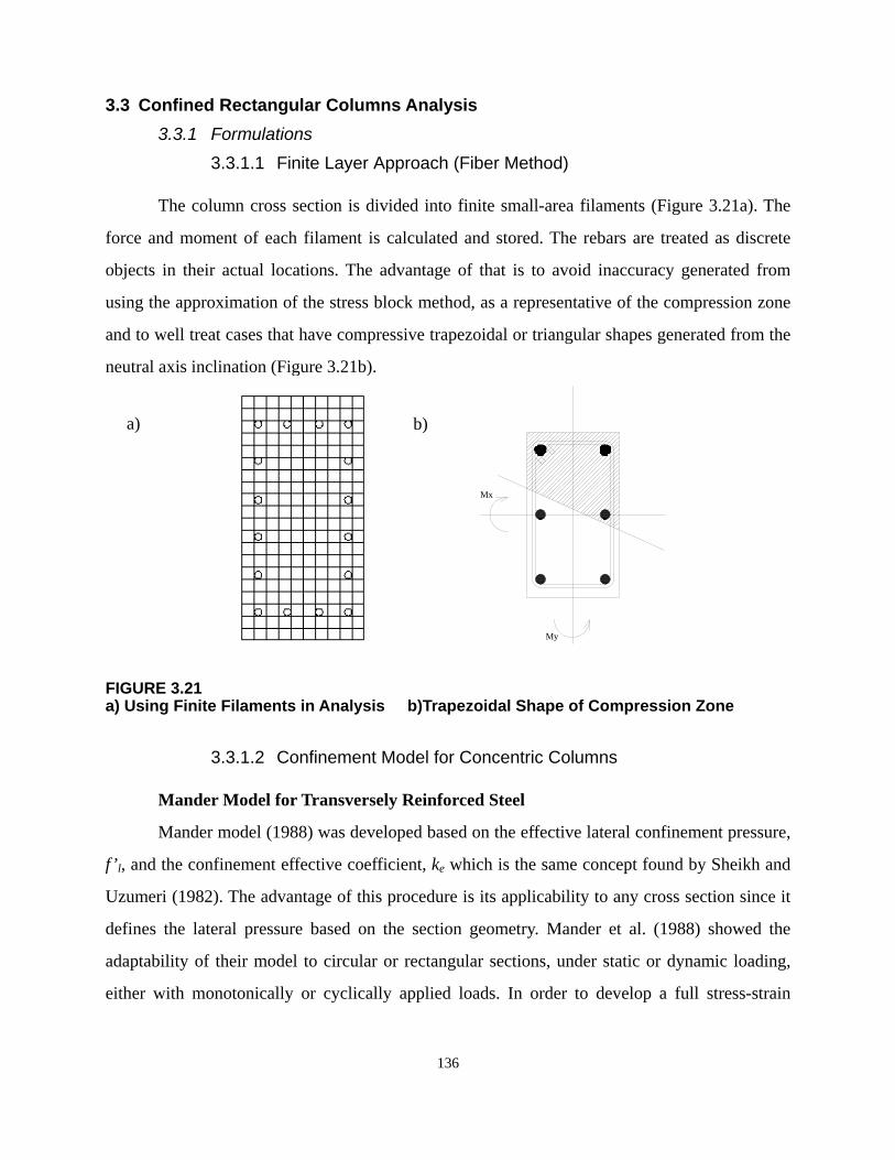
136
3.3 Confined Rectangular Columns Analysis
3.3.1 Formulations
3.3.1.1 Finite Layer Approach (Fiber Method)
The column cross section is divided into finite small-area filaments (Figure 3.21a). The
force and moment of each filament is calculated and stored. The rebars are treated as discrete
objects in their actual locations. The advantage of that is to avoid inaccuracy generated from
using the approximation of the stress block method, as a representative of the compression zone
and to well treat cases that have compressive trapezoidal or triangular shapes generated from the
neutral axis inclination (Figure 3.21b).
Mx
My
FIGURE 3.21 a) Using Finite Filaments in Analysis b)Trapezoidal Shape of Compression Zone
3.3.1.2 Confinement Model for Concentric Columns
Mander Model for Transversely Reinforced Steel
Mander model (1988) was developed based on the effective lateral confinement pressure,
f’l, and the confinement effective coefficient, ke which is the same concept found by Sheikh and
Uzumeri (1982). The advantage of this procedure is its applicability to any cross section since it
defines the lateral pressure based on the section geometry. Mander et al. (1988) showed the
adaptability of their model to circular or rectangular sections, under static or dynamic loading,
either with monotonically or cyclically applied loads. In order to develop a full stress-strain
a) b)

137
curve and to assess ductility, an energy balance approach is used to predict the maximum
longitudinal compressive strain in the concrete.
Mander derived the longitudinal compressive concrete stress-strain equation from
Popovics model that was originally developed for unconfined concrete (1973):
rcc
c xr
xrff
1 Equation 3.67
cc
cx
Equation 3.68
secEE
Er
c
c
Equation 3.69
'4723 cc fE in MPa Equation 3.70
cc
ccfE
sec Equation 3.71
and as suggested by Richart et al. (1928) the strain corresponding to the peak confined
compressive strength, f’cc, is:
151
'c
cccocc f
f Equation 3.72
The different parameters of this model are defined in Figure 3.22.

138
Com
pres
sive
Str
ess
Unconfined Concrete
Confined Concrete
First HoopFracture
fcc
f'c
co co sp cc cu
Ec Esec
FIGURE 3.22 Axial Stress-Strain Model Proposed by Mander et al. (1988) for Monotonic Loading
As shown in Figure 3.22 Mander et al. (1988) model has two curves; one for unconfined
concrete (lower curve) and the other for confined concrete (upper one). The upper one refers to
the behavior of confined concrete with concentric loading (no eccentricity). It is shown that it has
ascending branch with varying slope starting from Ec decreasing till it reaches the peak confined
strength at (fcc, cc). Then the slope becomes slightly negative in the descending branch
representing ductility till the strain of cu where first hoop fractures. The lower curve expresses
the unconfined concrete behavior. It has the same ascending branch as the confined concrete
curve till it peaks at (f’c, co). Then, the curve descends till 1.5-2co. A straight line is assumed
after that till zero strength at spalling strain sp.
Mander et al. (1988) utilized an approach similar to that of Sheik and Uzumeri (1982) to
determine effective lateral confinement pressure. It was assumed that the area of confined
concrete is the area within the centerlines of perimeter of spiral or hoop reinforcement Acc as
illustrated in Figure 3.23.

139
45° s's
Effectively Confined Core
Effectively Confined Core
45°
Smallest Lengthfor Confined Core
FIGURE 3.23 Effectively Confined Core for Rectangular Hoop Reinforcement (Mander Model)
Figure 3.23 shows that effectively confined concrete core Ae is smaller than the area of
core within center lines of perimeter spiral or hoops excluding longitudinal steel area, Acc, and to
satisfy that condition the effective lateral confinement pressure f’l should be a percentage of the
lateral pressure fl:
lel fkf ' Equation 3.73
and the confinement effectiveness coefficient ke is defined as the ratio of the effective
confined area Ae to the area enclosed by centerlines of hoops excluding the longitudinal bars Acc:
cc
ee A
Ak Equation 3.74
slccc AAA Equation 3.75
c
sl
c
cc
A
A
A
A 1 Equation 3.76
ccccc AA 1 Equation 3.77

140
where Ac is the area of the section core enclosed by hoops, Asl is the area of longitudinal steel and
cc is the ratio of longitudinal steel to the area of the core.
bc-s'/2
bc
s' s
bc
dcdc-s'/2
w'
Effectively Confined Core
Ineffectively Confined Core
B
H
FIGURE 3.24 Effective Lateral Confined Core for Rectangular Cross Section
The total ineffective confined core area in the level of the hoops when there are n bars:
n
i
ii
wA
1
2'
6 Equation 3.78
Given that the arching formed between two adjacent bars (Figure 3.24) is second degree
parabola with an initial tangent slope of 45o, the ratio of the area of effectively confined concrete
to the core area at the tie level:
et
n
i
iet
A
wA
1
2'
6 Equation 3.79

141
where Ac = bc* dc, The area of confined concrete in the midway section between two consecutive
ties:
ccccccemt d
s
b
sdb
sd
sbA
21
21
22
''''
Equation 3.80
Hence, the effective area at midway:
cccc
n
i
icc
cccccce d
s
b
sdb
wdb
dbd
s
b
sdbA
21
21
6
1
21
21
''
1
2'''
Equation 3.81
cc
n
i
icce d
s
b
swdbA
21
21
6
''
1
2'
Equation 3.82
Using Equation 3.73
cccc
cc
n
i cc
icc
e db
d
s
b
s
db
wdb
k
1
21
21
61
''
1
2'
Equation 3.83
cc
cc
n
i cc
i
e
d
s
b
s
db
w
k
1
21
21
61
''
1
2'
Equation 3.84
and the ratio of the volume of transverse steel in x any y directions to the volume of
confined core area x and y is defined as:
c
sx
cc
csxx sd
A
dsb
bA Equation 3.85
c
sy
cc
csyy sb
A
dsb
dA Equation 3.86

142
Asx, Asy are the total area of lateral steel in x and y direction respectively. The effective
lateral confining pressure in x and y directions are given by:
yhxelx fkf ' Equation 3.87
yhyely fkf ' Equation 3.88
Lar
gest
con
fini
ng S
tres
s ra
tio
Largest confining Stress ratio
0 0.30.1 0.20.3
0.2
0.1
0 1.0 2.01.5
Confined Strength ratio f'cc/f'co
f'l1/f'co
f'l2/
f'co
FIGURE 3.25 Confined Strength Determination

143
Figure 3.25 was developed numerically using multiaxial stress procedure to calculate
ultimate confined strength from two given lateral pressures. The numerical procedure is
summarized in the following steps:
1. Determining f’lx and f’ly using Equations 3.86 and 3.87
2. Converting the positive sign of f’lx and f’ly from positive to negative to represent
the major and intermediate principal stresses (These values are referred to as 1
and 2 so that 1 > 2).
3. Estimating the confined strength f cc (3) as the minor principal stress
4. Calculating the octahedral stress oct, octahedral shear stress oct and lode angle
as follows:
3213
1 oct Equation 3.89
21213
232
2213
1 oct Equation 3.90
oct
oct
2
cos 1
Equation 3.91
1. Determining the ultimate strength meridian surfaces T,C (for =60o and 0o
respectively) using the following equations derived by Elwi and Murray (1979)
from data by Scickert and Winkler (1977):
2
0.069232 0.661091 0.049350oct octT
Equation 3.92
2
0.122965 1.150502 0.315545oct octC Equation 3.93
'/oct oct cf Equation 3.94

144
2. Determining the octahedral shear stress using the interpolation function found by
Willam and Warnke (1975):
12 2
2
0.5 / cos 2 5 4
2oct
D T C D T TCC
D T C
Equation 3.95
2 2 24 cosD C T Equation 3.96
'coctoct f Equation 3.97
3. Recalculating f cc using the following equation (same as Equation 3.89) but
solving for 3:
221221
3 75.05.42
oct
Equation 3.98
4. If the value from Equation 3.97 is close to the initial value then there is
convergence. Otherwise, the value from Equation 3.97 is reused in steps 4
through 8.
Equations 3.91 and 3.92 that define the tension and compression meridians are compared
with different equations for different unconfined compressive strength. The results are shown in
section 3.3.3.2.
Mander et al. (1988) proposed an energy balancing theory to predict the ultimate
confined strain, which is determined at the first hoop fracture. They stated that the additional
ductility for confined concrete results from the additional strain energy stored in the hoops Ush.
Therefore from equilibrium:
cogsh UUU Equation 3.99
145
where Ug is the external work done in the concrete to fracture the hoop, and Uco is the work done
to cause failure to the unconfined concrete. Ush can be represented by the area under the tension
stress strain curve for the transverse steel between zero and fracture strain sf.
dfAUsf
sccssh 0
Equation 3.100
while Ug is equal to the area under the confined stress strain curve plus the area under the
longitudinal steel stress strain curve:
dAfdAfUscuscu
slscccg 00
Equation 3.101
similarly, it was proven experimentally that Uco is equal to:
'
0
017.0 ccccccco fAdfAUspall
in MPa Equation 3.102
and
ccssccssh AdfAUsf
1100
Equation 3.103
Substituting Equations 3.100, 3.101, and 3.102 into Equation 3.98:
'
00
017.0110 cslcs fdfdfcucu
Equation 3.104
where fsl is the stress in the longitudinal steel. Equation 3.103 can be solved numerically for cu.

146
3.3.1.3 Confinement Model for Eccentric Columns
Unlike concentric loading, the eccentric loading generates bending moment in addition to
axial loading. Columns subjected to eccentric loading behave differently from those
concentrically loaded, as the shape of the stress strain curve for fully confined reinforced
concrete (concentric loading) shows higher peak strength and more ductility than the unconfined
one (infinite eccentricity). Most of the previous studies were based on the uniform distribution of
compressive strain across the column section.
FIGURE 3.26 Effect of Compression Zone Depth on Concrete Stress
Figure 3.26 illustrates three different sections under concentric load, combination of axial
load and bending moment and pure bending moment, the highlighted fiber in the three cases has
the same strain. Any current confinement model yields the same stress for these three fibers. So
the depth or size of compression zone does not have any role in predicting the stress. Hence, it is
more realistic to relate the strength and ductility in a new model to the level of confinement
utilization and compression zone size.

147
FIGURE 3.27 Amount of Confinement Engaged in Different Cases
By definition, confinement gets engaged only when member is subjected to compression.
Compressed members tend to expand in lateral direction, and if confined, confinement will
prevent this expansion to different levels based on the degree of compressive force and
confinement strength as well. For fully compressed members (Figure 3.27), confinement
becomes effective 100% as it all acts to prevent the lateral expansion. Whereas members
subjected to compression and tension, when the neutral axis lies inside the section perimeter,
only confinement adjacent to the compression zone gets engaged. Accordingly, members become
partially confined.
In literature, various models were implemented to assess the ultimate confined capacity
of columns under concentric axial load. On the other hand the effect of partial confinement in
case of eccentric load (combined axial load and bending moments) is not investigated in any
proposed model. Therefore, it is pertinent to relate the strength and ductility of reinforced
concrete to the degree of confinement utilization in a new model.
The two curves of fully confined and unconfined concrete in any proposed model are
used in the eccentricity-based model as upper and lower bounds. The upper curve refers to
concentrically loaded confined concrete (zero eccentricity), while the lower one refers to pure
bending applied on concrete (infinite eccentricity). In between the two boundaries, infinite
numbers of stress-strain curves can be generated based on the eccentricity. The higher the
eccentricity the smaller the confined concrete region in compression. Accordingly, the ultimate
confined strength is gradually reduced from the fully confined value fcc to the unconfined value
f’c as a function of eccentricity to diameter ratio. In addition, the ultimate strain is gradually

148
reduced from the ultimate strain cu for fully confined concrete to the ultimate strain for
unconfined concrete 1.5co.
The relation between the compression area to whole area ratio and normalized
eccentricity is complicated in case of rectangular cross sections due to the existence of two
bending axes. The force location with respect to the two axes causes the compression zone to
take a trapezoidal shape sometimes if the force applied is not along one of the axes. Hence the
relation between the compression area and the load eccentricity needs more investigation as
oppose to the case of circular cross section which was shown to be simpler.
The normalized eccentricity is plotted against the compression area to cross sectional area
ratio for rectangular cross sections having different aspect ratio (length to width) at the
unconfined failure level. The aspect ratios used are 1:1, 2:1, 3:1, 4:1 as shown in Figures 3.28,
3.29, 3.30, and 3.31. Each curve represents specific angle (tan = My/Mx) ranging from zero
to ninety degrees. It is seen from these figures that there is inversely proportional relation
between the normalized eccentricity and compression zone ratio regardless of the angle
followed.
FIGURE 3.28 Normalized Eccentricity versus Compression Zone to Total Area Ratio
0
20
40
60
80
100
120
0 5 10 15 20 25 30 35
Compression area to the cross sectional area
ratio
eccentricity/(bh)^0.5
Aspect ratio 1:1
0
10
20
30
40
50
60
70
80
90
angles

149
(Aspect Ratio 1:1)
FIGURE 3.29 Normalized Eccentricity versus Compression Zone to Total Area Ratio (Aspect Ratio 2:1)
FIGURE 3.30 Normalized Eccentricity versus Compression Zone to Total Area Ratio (Aspect Ratio 3:1)
0
20
40
60
80
100
120
0 0.5 1 1.5 2 2.5
Compression area to the cross sectional
area ratio
eccentricity/(bh)^0.5
Aspect ratio 2:1
0103030405060708090
0
20
40
60
80
100
120
0 0.5 1 1.5 2
Compression area to the cross sectional area
ratio
eccentricity/(bh)^0.5
Aspect ratio 3:1
0102030405060708090
angles
angles

150
FIGURE 3.31 Normalized Eccentricity versus Compression Zone to Total Area Ratio (Aspect Ratio 4:1)
FIGURE 3.32 Cumulative Chart for Normalized Eccentricity against Compression Zone Ratio (All Data Points)
0
20
40
60
80
100
120
0 0.5 1 1.5 2
Compression area to the cross sectional
area ratio
eccentricity/(bh)^0.5
Aspect ratio 4:1
0102030405060708090
0
20
40
60
80
100
120
0 0.5 1 1.5 2 2.5
Compression area to the cross sectional
area ratio
eccentricity/(bh)^0.5

151
In order to find accurate mathematical expression that relates the compression zone to
load eccentricity, the data from Figures 3.28 through 3.31 are replotted as scatter points in Figure
3.32.
The best fitting curve of these points based on the least square method has the following
equation:
bh
ebh
e
CR
1.0*2.0
Equation 3.105
where CR refers to compression area to cross sectional area ratio.
Eccentric Model based on Mander Equations
The equation that defines the peak strength ccf according to the eccentricity is:
'
1
11
1
1c
Rcc
R
cc fC
f
C
f
Equation 3.106
whereas the equation developed for circular cross sections
'
1
1
1
1ccccc f
e
bhf
bh
ef
Equation 3.107
where e is the eccentricity, b and h is the column dimensions and ccf is the peak strength at the
eccentricity (e). The corresponding strain cc is given by
151
'c
cccocc
f
f Equation 3.108

152
and the maximum strain corresponding to the required eccentricity will be a linear
function of stress corresponding to maximum strain for confined concrete fcu and the maximum
unconfined concrete fcuo at cuo = 0.003:
r
cu
ucccu r
c
rE
E1
sec,
sec
11
003.0sec,
cu
cuocuu
ffE
Equation 3.109
u
ucu
E
Efc
sec,
sec, 003.0*
cc
ccfE
sec
secEE
Er
c
c
Equation 3.110
In order to verify the accuracy of the model at the extreme cases, the eccentricity is first
set to be zero. The coefficient of f’c will be zero in Equation 3.105 and Equations 3.105, 3.106
and 3.107 will reduce to be:
cccc ff Equation 3.111
cccc Equation 3.112
cucu Equation 3.113
On the other hand, if the eccentricity is set to be infinity the other coefficient will be zero,
and the strength, corresponding strain and ductility equations will be:
'
ccc ff Equation 3.114
cocc Equation 3.115
003.0cu Equation 3.116

153
Com
pres
sive
Str
ess
Compressive Strain
Unconfined Concrete
Confined Concretefcc
f'c
co sp cc cu cu
fcc
cc
Partially Confined Concrete
FIGURE 3.33 Eccentricity Based Confined Mander Model
Any point on the generated curves the stress-strain function can be calculated using the
following equation:
r
ccc
xr
rxff
1 Equation 3.117
where:
cc
cx
Equation 3.118
secEE
Er
c
c
Equation 3.119
cc
ccfE
sec Equation 3.120
To show the distinction between the Eccentric model designed for rectangular cross
sections, Figure 3.34 and that of circular cross sections, Figure 3.35, Equations 3.105 to 3.107

154
and 3.114 to 3.117 are used in plotting a set of Stress-Strain curves with eccentricity ranging
from 0 inches to ∞. The column cross sectional properties used to plot these curves is 36 in *36
inches, steel bars are 13 #11, spiral bar is # 5, spacing is 4 inches, f’c is equal to 4 ksi, fy is equal
to 60 ksi and fyh is equal to 60 ksi. This case is used in plotting the Eccentric Stress-Strain curve
that are developed for rectangular cross sectional concrete columns; Figure 3.34 while the same
case is used in plotting the eccentric Stress-Strain curves that are developed for circular cross
section, Figure 3.35. The eccentric stress-Strain curves in Figure 3.35 are almost parallel and
equidistant to each other. Whereas, the leap from one curve to the next one in Figure 3.34 is
varying. This is due to the effect of the coefficient CR, that is used in Equation 3.105, which has
non linear impact on the compression zone as opposed to the linear relation between the
eccentricity and compression zone for circular cross sections (Figure 3.35)
FIGURE 3.34 Eccentric Based Stress-Strain Curves Using Compression Zone Area to Gross Area Ratio
0
1
2
3
4
5
6
0 0.01 0.02 0.03
Axi
al S
tres
s (k
si)
Axial Strain
e = 0 in
e = 1 in
e = 2 in
e = 3 in
e = 4 in
e = 5 in
e = 6 in
e = 7 in
e = 8 in
e = 9 in
e = infiniti

155
FIGURE 3.35 Eccentric Based Stress-Strain Curves Using Normalized Eccentricity Instead of Compression Zone Ratio
3.3.1.4 Generalized Moment of Area Theorem
The very general axial stress equation in an unsymmetrical section subjected to axial
force P and biaxial bending Mx and My (Hardy Cross 1930):
xIII
IMIMy
III
IMIM
A
P
xyyx
xyxxy
xyyx
xyyyxz 22
Equation 3.121
z = normal stress at any point (a) in cross section
P = applied load.
A = cross sectional area.
xM = bending moment about x-axis
yM = bending moment about y-axis
x = distance between the point (a) and y-axis
0
1
2
3
4
5
6
0 0.005 0.01 0.015 0.02 0.025 0.03 0.035
Axi
al S
tres
s (k
si)
Axial Strain
e = 0 in
e = 1 in
e = 2 in
e = 3 in
e = 4 in
e = 5 in
e = 6 in
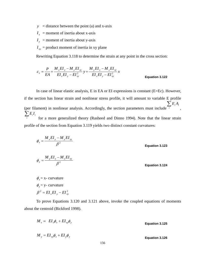
156
y = distance between the point (a) and x-axis
xI = moment of inertia about x-axis
yI = moment of inertia about y-axis
xyI = product moment of inertia in xy plane
Rewriting Equation 3.118 to determine the strain at any point in the cross section:
xEIEIEI
EIMEIMy
EIEIEI
EIMEIM
EA
P
xyyx
xyxxy
xyyx
xyyyxz 22
Equation 3.122
In case of linear elastic analysis, E in EA or EI expressions is constant (E=Ec). However,
if the section has linear strain and nonlinear stress profile, it will amount to variable E profile
(per filament) in nonlinear analysis. Accordingly, the section parameters must include
iii AE,
i
ii IE for a more generalized theory (Rasheed and Dinno 1994). Note that the linear strain
profile of the section from Equation 3.119 yields two distinct constant curvatures:
2 xyyyx
x
EIMEIM
Equation 3.123
2 xyxxy
y
EIMEIM
Equation 3.124
x = x- curvature
y = y- curvature 22xyyx EIEIEI
To prove Equations 3.120 and 3.121 above, invoke the coupled equations of moments
about the centroid (Bickford 1998).
yxyxxx EIEIM Equation 3.125
yyxxyy EIEIM Equation 3.126

157
In a matrix form:
y
x
yxy
xyx
y
x
EIEI
EIEI
M
M
Equation 3.127
Inverting Equation 3.124
y
x
xxy
xyy
y
x
M
M
EIEI
EIEI2
1
Equation 3.128
which reproduces Equations 3.120 and 3.121. Rewriting Equation 3.119 in terms of x
and y
xyEA
Pyxz
Equation 3.129
Finding z at the centroid, since x = y = 0.
P/EA = o
Equation 3.130
Solving for P at the geometric centroid;
yxo xEAyEAEAP Equation 3.131
o is the axial strain at the geometric centroid
But
yEAEAM x
cG YYy
xEAEAM y
cG XXx

158
YG is the vertical distance to the geometric centroid measured from bottom, XG is the
distance to the geometric centroid measured from the cross section’s left side, Yc is the vertical
distance to the inelastic centroid measured from the bottom and Xc is the horizontal distance to
the inelastic centroid measured from the cross section’s left side
Thus,
yyxxo EAMEAMEAP Equation 3.132
The general formula of the moments about the geometric x-axis and the geometric y-axis
is derived as follows:
when the moment is transferred from the centroid to the geometric centroid (Figure
3.36a)
yPMM xx Equation 3.133
Substituting Equations 3.122 and 3.129 into 3.130 yields:
yEAMyEAMyEAEIEIM yyxxoyxyxxx
Equation 3.134
yyxyxxxoxx yEAMEIyEAMEIEAMM Equation 3.135
Similarly, Figure 3.36b:

159
G
Cy
P
Mx
Mx GC
P
MyMy
xyyG
cx
xc
G
FIGURE 3.36 Transferring Moment from Centroid to the Geometric Centroid
xPMM yy Equation 3.136
xEAMxEAMxEAEIEIM yyxxoyyxxyy Equation 3.137
yyyxxxyoyy xEAMEIxEAMEIEAMM Equation 3.138
The terms yEAMEI xx and xEAMEI yy represent the xEI and yEI
about the
geometric centroid respectively using the parallel axis theorem. And the terms xEAMEI xxy
and yEAMEI yxy are equal given that: xyEAxEAM x and
xyEAyEAM y . Using
Equations 3.129, 3.132 and 3.135 yields the extended general moment of area equation:
y
x
yxyy
xyxx
yx
y EIEIEAM
EIEIEAM
EAMEAMEA
M
Mx
P
Equation 3.139
Since the moment of area about the centroid vanishes (Rasheed and Dinno 1994),
Equation 3.136 reduces to a partially uncoupled set when it is applied back at the centroid since
EAMx and EAMy vanish about the centroid.
a) b)

160
y
x
o
yxy
xyx
y
x
EIEI
EIEI
EA
M
M
P
0
0
00
Equation 3.140
which is simply Equations 3.122, 3.123, and 3.127
3.3.2 Numerical Formulation
This approach simulates the radial loading of the force and moments by keeping the
relative proportion between them constant during the loading. Accordingly, all the points will be
exactly on the 2D interaction diagram. In addition to the ultimate points, the complete load
deformation response is generated. The cross section analyzed is loaded incrementally by
maintaining a certain eccentricity between the axial force P and the resultant moment MR. Since
MR is generated as the resultant of Mx and My, the angle = tan-1(My/Mx) is kept constant for a
certain 2D interaction diagram. Since increasing the load and resultant moment cause the neutral
axis to vary nonlinearly, the generalized moment of area theorem is devised. This method is
based on the general response of rectangular unsymmetrical section subjected to biaxial bending
and axial compression. The asymmetry stems from the different behavior of concrete in
compression and tension.
The method is developed using the incremental iterative analysis algorithm, secant
stiffness approach and proportional or radial loading. It is explained in the following steps Figure
3.40:
1. Calculating the initial section properties:
Elastic axial rigidity EA:
Equation 3.141
= initial secant modulus of elasticity of the concrete
= initial modulus of elasticity of the steel rebar
i
sicsiii
c AEEtwEEA )(
cE
sE

161
The depth of the elastic centroid position from the bottom fiber of the section
Yc and from the left side of the section Xc, Figure 3.37
Equation 3.142
EA
XBAEEXBtwEX i i
sisicsiiic
c
)()()(
Equation 3.143
Elastic flexural rigidity about the elastic centroid EI:
Equation 3.144
22 )()()( csisici
sciiii
cy XXHAEEXXBtwEEI Equation 3.145
cicsisici
sciciiii
cxy XXBYYHAEEXXBYYHtwEEI )()()(
Equation 3.146
Typically the initial elastic Yc = H/2, Xc = B/2 and EIxy = 0
EA
YHAEEYHtwEY i i
sisicsiiic
c
)()()(
22 )()()( csisici
sciiii
cx YYHAEEYYHtwEEI

162
Yi
H
Yc
B
Xc
Xi
wt
C
G
X
Y
G
G
0.003
H
Yc
B
Xc
Xsi
Ysi
X
Y
0.003
0.003 0.003
C
G
G
G
FIGURE 3.37 Geometric Properties of Concrete Filaments and Steel Rebars with Respect to Crushing Strain Point, Geometric Centroid and Inelastic Centroid
The depth of the geometric section centroid position from the bottom and left fibers of
the section YG, XG, Figure 3.37:
Equation 3.147
2
BX G
Equation 3.148
2. Defining eccentricity e, which specifies the radial path of loading on the
interaction diagram. Also, defining the angle in between the resultant moment
GMR and GMX
2
HYG

163
FIGURE 3.38 Radial Loading Concept
3. Defining loading step as a small portion of the maximum load, and
computing the axial force at the geometric centroid.
Equation 3.149
4. Calculating moment GM about the geometric centroid.
GP
GMe R GPeGM R * Equation 3.150
cosRX GMGM Equation 3.151
tanXY GMGM Equation 3.152
5. Transferring moment to the current inelastic centroid and calculating the new
transferred moment TMX and TMY :
)( cGXX YYGPGMTM
Equation 3.153
e
Resultant Moment
Axi
al F
orce
Load Step GP
GP
GPGPGP oldnew

164
)( cGYY XXGPGMTM Equation 3.154
The advantage of transferring the moment to the position of the inelastic centroid is to
eliminate the coupling effect between the force and moments, since 0 yx EAMEAM about
the inelastic centroid
y
x
o
yxy
xyx
y
x
EIEI
EIEI
EA
TM
TM
P
0
0
00
Equation 3.155
YG
XGXc
Yc
FIGURE 3.39 Moment Transferring from Geometric Centroid to Inelastic Centroid
6. Finding: Curvatures X and Y
XYY
YX
X EITM
EITM
**22
Equation 3.156
XYX
XY
Y EITM
EITM
**22
Equation 3.157
22xyYX EIEIEI Equation 3.158

165
Strain at the inelastic centroid , the extreme compression fiber strain , and strain at
the extreme level of steel in tension are found as follow:
Equation 3.159
)()( cycxoec XBYH Equation 3.160
)()( CoverXCoverY cycxoes Equation 3.161
where cover is up to the centers of bars
7. Calculating strain and corresponding stress fci in each filament of concrete
section by using Eccentric Based Model (Mander Equations)
xy
icyxy
icx
xicy
yicx
ci
EIYYHTM
EIXXBTM
EIXXBTM
EIYYHTM
EA
GP
22
22
Equation 3.162
8. Calculating strain and corresponding stress fsi in each bar in the given section
by using the steel model shown in Figure 3.2b.
xy
sicyxy
sicx
xsicy
ysicx
si
EIYYHTM
EIXXBTM
EIXXBTM
EIYYHTM
EA
GP
22
22
Equation 3.163
9. Calculating the new section properties: axial rigidity EA, flexural rigidities about
the inelastic centroid EIx,, EIy, EIxy moment of axial rigidity about inelastic
o ec
es
EA
GPo
ci
si

166
centroid EAMx, EAMy, internal axial force Fz, internal bending moments about the
inelastic centroid Mox ,Moy:
i
sicisiiii
ci AEEtwEEA )( Equation 3.164
)()()( sicsicii
siiciii
cix YYHAEEYYHtwEEAM Equation 3.165
)()()( sicsicii
siiciii
ciy XXBAEEXXBtwEEAM Equation 3.166
sicisiiiciz AfftwfF )( Equation 3.167
22 )()()( sicsicii
siiciii
cix YYHAEEYYHtwEEI Equation 3.168
22 )()()( sicsicii
siiciii
ciy XXHAEEXXBtwEEI Equation 3.169
sicsicsicii
siiciciii
cixy XXBYYHAEEXXBYYHtwEEI )()()(
Equation 3.170
Equation 3.171
)()()( sicsicisiiciicioy XXBAffXXBtwfM Equation 3.172
where Eci = secant modulus of elasticity of the concrete filament .
Esi = secant modulus of elasticity of the steel bar .
10. Transferring back the internal moments about the geometric centroid
)()()( sicsicisiiciiciox YYHAffYYHtwfM

167
Equation 3.173
)( cGoyoy XYGPMGM Equation 3.174
11. Checking the convergence of the inelastic centroid
Equation 3.175
cyy XEAEAMTOL // Equation 3.176
12. Comparing the internal force to applied force, internal moments to applied
moments, and making sure the moments are calculated about the geometric
centroid :
510*1 zFGP Equation 3.177
510*1 oxx GMGM
510*1 oyy GMGM Equation 3.178
510*1 xTOL 510*1 yTOL
Equation 3.179
If Equations 3.174, 3.175 and 3.176 are not satisfied, the location of the inelastic centroid
is updated by EAMx/EA and EAMy/EA and steps 5 to 11 are repeated till Equations 3.174, 3.175
and 3.176 are satisfied.
Equation 3.180
EA
EAMXX y
cc oldnew
Equation 3.181
)( cGoxox YYGPMGM
cxx YEAEAMTOL //
EA
EAMYY x
cc oldnew

168
Once equilibrium is reached, the algorithm checks for ultimate strain in concrete and
steel not to exceed and 0.05 respectively. Then it increases the loading by and runs
the analysis for the new load level using the latest section properties. Otherwise, if equals
or equals 0.05, the target force and resultant moment are reached as a point on the failure
surface for the amount of eccentricity and angle used.
This method can be used combined with Approach One in the unconfined analysis,
section 3.2.2.1: Predefined Ultimate Strain Profile, for processing time optimization. Initially
unconfined analysis is utilized. The sectional properties, EA, EIx, EIy, EIxy, EAMx, EAMy,Yc,Xc Fz,
Mox and Moy are calculated from the unconfined failure point and used as section properties for
the following step. So instead of loading the section from the beginning, The equilibrium is
sought at unconfined failure point, Then, knowing the internal force capacity of the section, P
is added and the cross section is analyzed using the proposed numerical formulation of this
section until failure of the confined section.
ec
es GP
ec
es

169
S ta r t
C a lc u la te in it ia l s e c tio n p ro p e r t ie s
E A ,E I x , E I y,E I x y
Y c ,Y G ,X c ,X G
In p u t P ,
T ra n s fe r m o m e n t to in e la s tic c e n tro idT M x = G M x + P (Y G -Y c)T M y = G M y + P (X G -X c)
C a lc u la te ø x ,ø y , o , e c , e s
C a lc u la te c i, s i,f c i, f s i
C a lc u la te n e w s e c tio n p ro p e r tie s
E A ,E I x , E I y, E A M x,
E A M y
C a lc u la te in te rn a l fo rc e a n d m o m e n ts
F z,M ox ,M oy
T ra n s fe r m o m e n t b a c k to G .C .
G M o x = M o x -P (Y G -Y c)G M o y = M o y -P (X G -X c)
E A M xE A * Y c
1 0-5
E A M yE A * X c
1 0-5
Y c + = E A M x /E A
|G P -F z |<<
<
1 0-5
|G M x - G M o x|<1 0-5
|G M y - G M o y|< 1 0-5
P + = P
P & M a c h ie v e dN e w e c c in tr ic ity
E n d
y e s
y e s
n o
n o
y e s
n o
e &
,E I xy
X c + = E A M y /E A
e c > = c u
e s > = 0 .0 5
N o c o n v e rg e n c ea c h ie v e d . s to p
n o
y e s
N e w ay e s
n o
FIGURE 3.40 Flowchart of Generalized Moment of Area Method

170
3.3.3 Results and Discussion
Interaction diagrams generated by KDOT Column Expert Software are plotted and
compared to the corresponding experimental work found in the literature. Interaction diagrams
are generated using the numerical formulation described in section 3-3-2.
3.3.3.1 Comparison with Experimental Work Case 1
A Study of combined bending and axial load in reinforced concrete members (Eivind
Hogenstad)
Section Height = 10 inches
Section Width = 10 inches
Clear Cover = 0.8575 inches
Steel Bars in x direction = 2
Steel Bars in y direction = 4
Steel Diameter = 0.785 inches
Tie Diameter = 0.25 inches
f’c = 5.1 ksi fy = 60 ksi. fyh = 61.6 ksi. Spacing = 8 inches
FIGURE 3.41 Hognestad Column

171
FIGURE 3.42 Comparison between KDOT Column Expert with Hognestad Experiment ( = 0)
3.3.3.2 Comparison with Experimental Work Case 2
Design criteria for reinforced columns under axial load and biaxial bending (Boris
Bresler)
Section Height = 8 inches
SectionWidth = 6 inches
Clear Cover = 1.1875 inches
Steel Bars in x direction = 2#5
Steel Bars in y direction = 2#5
Tie Diameter = 0.25 inches

172
FIGURE 3.43 Bresler Column
f ’c = 3.7 ksi fy = 53.5 ksi. fyh = 53.5 ksi. Spacing = 4 in
FIGURE 3.44 Comparison between KDOT Column Expert with Bresler Experiment ( = 90)

173
FIGURE 3.45 Comparison between KDOT Column Expert with Bresler Experiment ( = 0)
3.3.3.3 Comparison with Experimental Work Case 3
Investigation of the ultimate strength of square and rectangular columns under biaxially
eccentric loads (L.N. Ramamurthy)
Section Height = 12 inches
Section Width = 6 inches
Clear Cover = 1.2375 inches
Steel Bars in x direction = 3#5
Steel Bars in y direction =3#5
Tie Diameter = 0.25 inches
f’c = 3.8 ksi fy = 46.79 ksi fyh = 46.79 ksi. Spacing = 6 inches

174
FIGURE 3.46 Ramamurthy Column
FIGURE 3.47 Comparison between KDOT Column Expert with Ramamurthy Experiment ( = 26.5)
3.3.3.4 Comparison with Experimental Work Case 4
Confined columns under eccentric loading
(Murat Saatcioglu. Amir Salamat and Salim Razvi )

175
Section Height = 8.27 inches
Section Width =8 .27 inches
Clear Cover = 0. 5 inches
Steel Bars in x direction = 3
Steel Bars in y direction = 3
Steel Area = 0.155 inches2
Tie Diameter = 0.364 inches
f’c = 5.1 ksi fy = 75 ksi. fyh = 59.45 ksi. Spacing = 1.97 inches
FIGURE 3.48 Saatcioglu Column
FIGURE 3.49 Comparison between KDOT Column Expert with Saatcioglu et al. Experiment ( = 0)
0
100
200
300
400
500
600
700
0 20 40 60
For
ce (
k.)
Moment (k.in.)
Experimental points
Interaction diagram " e relation"
Interaction diagram "CR relation"

176
3.3.3.5 Comparison with Experimental Work Case 5
Confined columns under eccentric loading
(Mural Saatcioglu. Amir Salamat and Salim Razvi )
Section Height = 8.27 inches
Section Width =8 .27 inches
Clear Cover = 0. 5 inches
Steel Bars in x direction = 4
Steel Bars in y direction = 4
Steel Area = 0.155 in2.
Tie Diameter = 0.364 inches
f’c = 5.1 ksi fy = 75 ksi. fyh = 59.45 ksi. Spacing = 1.97 inches
FIGURE 3.50 Saatcioglu Column

177
FIGURE 3.51 Comparison between KDOT Column Expert with Saatcioglu et al. Experiment 1 ( = 0)
3.3.3.6 Comparison with Experimental Work Case 6
Stress strain behavior of concrete confined by overlapping hoops at low and high strain
rate:
(B. Scott, R Park and M. Priestly)
Section Height = 17.7 inches
Section Width =17 .7 inches
Clear Cover = 0. 787 inches
Steel Bars in x direction = 4
Steel Bars in y direction = 4
Steel Area = 0.49 inches2
Tie Diameter = 0.394 inches
f’c = 3.67 ksi fy = 63 ksi. fyh = 44.8 ksi. Spacing = 2.83 inches
0
100
200
300
400
500
600
700
800
0 20 40 60 80
For
ce (
k.)
Moment (k.in.)
Experimental points
Interaction Diagram " e relation"
Interaction Diagram " CR relation"

178
FIGURE 3.52 Scott Column
FIGURE 3.53 Comparison between KDOT Column Expert with Scott et al. Experiment ( = 0)
0
200
400
600
800
1000
1200
1400
1600
1800
2000
0 100 200 300 400 500
For
ce (
k.)
Moment (k.in.)
Experimemtal points
Interaction diagram "e relation"
Interaction diagram "CR relation"
Interaction diagram "CR relation" with cover spalling
4
3
2

179
3.3.3.7 Comparison with Experimental Work Case Case 7
Stress strain behavior of concrete confined by overlapping hoops at low and high strain
rate
(B. Scott, R Park and M. Priestly)
Section Height = 17.7 inches
Section Width =17 .7 inches
Clear Cover = 0. 787 inches
Steel Bars in x direction = 3
Steel Bars in y direction = 3
Steel Area = 0.7 inches2.
Spiral Diameter = 0.394 inches
f’c = 3.67 ksi fy = 57.13 ksi. fyh = 44.8 ksi. Spacing = 2.83 inches
FIGURE 3.54 Scott Column

180
FIGURE 3.55 Comparison between KDOT Column Expert with Scott et al. Experiment ( = 0)
The analyzed seven cases cover the three Interaction diagram zones of; compression
controlled, tension controlled and balanced zones. There is good agreement between the
theoretical interaction diagram and the corresponding experimental data as shown in Figures
3.42, 3.44, 3.45, 3.47, 3.49, 3.51, 3.53, and 3.55.
It is shown from Figures 3.49, 3.51, 3.53, and 3.55 that interaction diagrams plotted using
Equation 3.105 that is representative of the compression zone area are more accurate compared
to those plotted using Equation 3.105a that is a function of eccentricity. Also the experimental
data correlate well to its associated interaction diagrams.
Figure 3.53 and 3.55 show more accuracy and conservative interaction diagram when the
analysis account for the cover spalling when the unconfined crushing strain is considered. This is
represented by the most inner curve in Figures 3.53 and 3.55. Also in Figure 3.53 and 3.55 the
experimental points 1 and 2 are having the same eccentricity but the loading strain rate is
different. The loading strain rate for point 1 is 0.0000033, whereas it is 0.0167 for point 2. Points
3 and 4 also have the same loading strain rate. It is seen that the loading strain rate for points 1
0
200
400
600
800
1000
1200
1400
1600
1800
2000
0 100 200 300 400 500
For
ce (
k.)
Moment (k.in.)
Experimental points
Interaction diagram "e relation"
Interaction diagram "CR relation"
Interaction diagram "CR relation" with cover spalling
3
2 4
1

181
and 3 are extremely small. Hence points 2 and 4 are more realistic and they are captured well by
the theoretical interaction diagram. In conclusion, the strain rate is a parameter that needs further
investigation.
3.3.3.8 Comparison between the Surface Meridians T&C Used in Mander
Model and Experimental Work
The ultimate strength surface meridians equations for compression C and tension T
derived by Elwi and Murray (1979) from the data of Scickert and Winkler (1977), that are
utilized by Mander et al. (1988) to predict the ultimate confined axial strength using the two
lateral confined pressures, are compared herein to some experimental data found from Mills and
Zimmerman (1970). The equations used by Mander are developed originally for concrete that
has unconfined strength of 4.4 ksi. They have the following formulas
2
049350.0661091.0069232.0 octoctT
Equation 3.182
2315545.0150502.1122965.0 octoctC Equation 3.183
FIGURE 3.56 T and C Meridians Using Equations 3.182 and 3.183 used in Mander Model for f’c = 4.4 ksi
y = ‐0.0493x2 ‐ 0.661x + 0.069
y = ‐0.3155x2 ‐ 1.15x + 0.122
0
0.2
0.4
0.6
0.8
1
1.2
‐1.5 ‐1 ‐0.5 0 0.5
oct
oct
T ( theta = 0)
C (theta = 60)
Poly. (T ( theta = 0))
Poly. (C (theta = 60))

182
The T and C meridians adopted by Mander from Elwi and Murray (1979) work are reported on
in Figure 3.56. Mills and Zimmerman (1970) developed three sets of multiaxial tests for concrete
with unconfined strength of 3.34, 3.9 and 5.2 ksi. For each set, the values of and are
extracted at unconfined strength f’c, the cracking tensile strength f’t, equibiaxial compressive
strength f’cb and two extra points; one on each of the meridians. These five points are used to plot
the T and C meridians as shown in Figures 3.57, 3.58 and 3.59.
FIGURE 3.57 T and C Meridians for f’c = 3.34 ksi
y = ‐0.0169x2 ‐ 0.6172x + 0.0851
y = ‐0.1865x2 ‐ 1.0471x + 0.1431
0
0.2
0.4
0.6
0.8
1
1.2
‐2 ‐1.5 ‐1 ‐0.5 0 0.5
oct
oct
T ( theta = 0)
C ( theta = 0)
Poly. (T ( theta = 0))
Poly. (C ( theta = 0))

183
FIGURE 3.58 T and C Meridians for f’c = 3.9 ksi
FIGURE 3.59 T and C Meridians for f’c = 5.2 ksi
The T and C equations for Figures 3.57 through 3.59 are as follow:
for f’c = 3.34 ksi:
y = ‐0.0151x2 ‐ 0.6479x + 0.0825
y = ‐0.112x2 ‐ 1.0472x + 0.1348
0
0.2
0.4
0.6
0.8
1
1.2
‐1.5 ‐1 ‐0.5 0 0.5
oct
oct
T ( theta = 0)
C ( theta = 60)
Poly. (T ( theta = 0))
Poly. (C ( theta = 60))
y = ‐0.0603x2 ‐ 0.6658x + 0.0719
y = ‐0.2768x2 ‐ 1.1332x + 0.1244
0
0.1
0.2
0.3
0.4
0.5
0.6
0.7
0.8
0.9
‐1 ‐0.5 0 0.5
oct
oct
T ( theta = 0)
C ( theta = 60)
Poly. (T ( theta = 0))
Poly. (C ( theta = 60))

184
20169.06172.00851.0 octoctT Equation 3.184
21865.00471.11431.0 octoctC Equation 3.185
for f’c = 3.9 ksi:
2
0151.06479.00825.0 octoctT Equation 3.186
2112.00472.11348.0 octoctC Equation 3.187
for f’c = 5.2 ksi:
2
0603.06658.00719.0 octoctT Equation 3.188
22768.01332.11244.0 octoctC Equation 3.189
Equations 3.181 through 3.186 are used in generating confined strength values for
different lateral pressures as shown in Appendix A. Equations 3.179 and 3.180 are used also in
developing confined strength values for the same lateral pressure values. It is seen from the
tables that Equations 3.179 and 3.180 give conservative values compared to Equations 3.181
through 3.186. Accordingly, Equations 3.179 and 3.180 are used herein to predict the ultimate
confined axial strength values for any given unconfined strength (f’c) value.
TABLE 3.1 Data for Constructing T and C Meridian
Curves for f’c Equal to 3.34 ksi
Control Parameter � Oct � Oct
f'c= 3.34 ksi -0.33333 0.471405
f't 0.043258 0.061176
f'cb -0.81497 0.576271
triaxial on C -1.15968 1.10653
triaxial on T -1.50898 0.978094

185
TABLE 3.2 Data for Constructing T and C Meridian
Curves for f’c Equal to 3.9 ksi
Control Parameter � Oct � Oct
f'c= 3.9 ksi -0.33333 0.471405
f't 0.040006 0.056578
f'cb -1.0904 0.771027
triaxial on C -1.06018 1.119058
triaxial on T -1.26248 0.876414
TABLE 3.3
Data for Constructing T and C Meridian Curves for f’c Equal to 5.2 ksi
Control Parameter � Oct � Oct
f'c= 5.2 ksi -0.33333 0.471405
f't 0.034553 0.048865
f'cb -0.80229 0.567306
triaxial on C -0.68386 0.76993
triaxial on T -0.88634 0.614725

186
Chapter 4: Conclusions and Recommendations
4.1 Conclusions
This study accomplished several objectives at the analysis, material modeling, design
implications and software development levels. It may be concluded that:
1. Based on the extensive review of the confined model available in the literature,
Mander Model is found to be the most suitable concentric loading model
expressing the stress-strain behavior of circular and rectangular columns confined
with convenient lateral steel and steel tubes as well.
2. The eccentric based stress-strain model developed in this study provides more
accuracy compared to the available concentric confined models in the literature as
it is shown through comparison with experimental data.
3. For rectangular columns, the ratio of the area of compression zone to the sectional
gross area is more representative than the normalized alone eccentricity in
correlating eccentric behavior.
4. The non-linear numerical procedure introduced, using the eccentric model and the
finite layer approach, successfully predicted the ultimate capacity of rectangular
reinforced concrete columns confined with steel.
5. A computer program named “KDOT Column Expert” is developed based on the
non-linear approach implemented for analyzing and designing rectangular
columns confined with lateral steel hoops.
6. The unconfined concrete analysis carried out by KDOT Column Expert is
benchmarked successfully against well-established commercial software for a
range of design parameters.
7. The confined concrete analysis implemented by KDOT Column Expert is well
correlated to experimental data.
4.2 Recommendations
This work should be extended to address the following areas:
1. Model the effect of FRP wrapping on confinement for rectangular columns.

187
2. Model corrosion of longitudinal and transverse steel for circular and rectangular
columns.
3. Model CFST for circular columns.
4. Model CFST for rectangular columns.
5. Expand the software application to include the CFST columns.

188
References
Aas-Jakobsen, A. 1964. “Biaxial Eccentricities in Ultimate Load Design.” ACI Journal 61 (3): 293–316.
ACI-ASCE Committee 327. 1956. “Ultimate Strength Design.” ACI Journal, Proceedings 52: 505–524.
Ahmad, S. H., and Shah, S. P. 1982. “Complete Triaxial Stress-Strain Curves for Concrete.” ASCE Journal 108 (ST4): 728–743.
Ahmad, S. H., and Shah, S. P. 1982. “Stress-Strain Curves of Concrete Confined by Spiral Reinforcement.” ACI Journal 79 (6): 484–490.
Andersen, Paul. 1941. “Design Diagrams for Square Concrete Columns Eccentrically Loaded in Two Directions.” ACI Journal, Proceedings 38: 149.
Ang, Cho-Lim Charles. 1961. “Square Column with Double Eccentricities Solved by Numerical Method.” ACI Journal, Proceedings 57: 977.
Assa B., Nishiyama, M., and Watanabe, F. 2001. “New Approach for Modeling Confined Concrete. I: Circular Columns.” Journal of Structural Engineering, ASCE 127 (7): 743–750.
Attard, M. M., and Setunge, S. 1996. “Stress-Strain Relationship of Confined and Unconfined Concrete.” ACI Materials Journal 93 (5): 432–442.
Au, Tung. 1957. “Ultimate Strength Design Charts for Columns Controlled by Tension.” ACI Journal, Proceedings 54: 471.
Au, Tung. 1958. “Ultimate Strength Design of Rectangular Concrete Members Subjected to Unsymmetrical Bending.” ACI Journal, Proceedings 54: 657.
Bajaj, S., and Mendis, P. 2005. “New Method to Evaluate the Biaxial Interaction Exponent for RC Columns.” Journal of Structural Engineering, ASCE 131 (12): 1926–1930.
Bakhoum, Michel. 1948. “Analysis of Normal Stresses in Reinforced Concrete Sections under Symmetrical Bending.” ACI Journal, Proceedings 44: 457.
Bazant, Z. P., and Bhat, P. D. 1976. “Endochronic Theory of Inelasticity and Failure of Concrete.” Journal of the Engineering Mechanics Division, ASCE 102 (4): 701–722.
Bazant, Z. P., and Bhat, P. D. 1977. “Prediction of Hysteresis of Reinforced Concrete Members.” Journal of the Structural Division, ASCE 103 (1): 153–167.
Binici, B. 2005. “An Analytical Model for Stress–Strain Behavior of Confined Concrete.” Engineering Structures 27 (7): 1040–1051.

189
Blume, J. A, Newmark, N. M., and Corning L. H. 1961. “Design of Multi Storey Reinforced Concrete Building for Earthquake Motions.” Chicago. Portland Cement Association.
Bonet, J. L., Barros, F. M., Romero, M. L. 2006. “Comparative Study of Analytical and Numerical Algorithms for Designing Reinforced Concrete Section under Biaxial Bending.” Computers and Structures 8:31–2.
Bonet, J. L., Miguel, P. F., Fernandez, M. A., and Romero, M. L. 2004. “Analytical Approach to Failure Surfaces in Reinforced Concrete Sections Subjected to Axial Loads and Biaxial Bending.” Journal of Structural Engineering 130 (12): 2006–2015.
Building Code Requirements for Reinforced Concrete. 1956. ACI 318-56. American Concrete Institute (ACI). Detroit, Michigan.
Braga, F., Gigliotti, R., Laterza, M. 2006. “Analytical Stress–Strain Relationship for Concrete Confined by Steel Stirrups and/or FRP Jackets.” Journal of Structural Engineering ASCE 132 (9): 1402–1416.
Breen, J. E. 1962. “The Restrained Long Concrete Column as a Part of A Rectangular Frame.” Ph. D. Thesis Presented to the University of Texas, Austin, TX.
Bresler, B. 1960. ‘‘Design, Criteria for Reinforced Columns under Axial Load Bi-Axial Bending.’’ ACI Journal Nov.: 481–491.
Bresler, B., and Gilberg, P. H. 1961. ‘‘Tie Requirements for Reinforced Concrete Columns.’’ ACI Journal 58 (5): 555–570.
Brettle, H. J.; Taylor, J. M. 1969. “Comparison of Experimental Results with Ultimate Strength Theory for Reinforced Concrete Columns in Biaxial Bending.” Transactions of the Institution of Engineers, Australia, Civil Engineering April 11 (1): 63–74.
Candappa, D. 2000. “The Constitutive Behavior of High Strength Concrete under Lateral Confinement.” PhD Thesis, Monash University, Clayton, VIC, Australia.
Candappa, D. P., Sanjayan, J. G., and Setunge, S. 2001. “Complete Triaxial Stress-Strain Curves of High-Strength Concrete.” Journal of Materials in Civil Engineering 13 (3): 209–215.
Candappa, D. P., Setunge, S., and Sanjayan, J. G. 1999. “Stress Versus Strain Relationship of High Strength Concrete under High Lateral Confinement.” Cement and Concrete Research 29 (12): 1977–1982.
Carreira, D J., and Chu, K. H. 1985. “Stress-Strain Relationship for Plain Concrete in Compression.” ACI Journal 83 (6): 797–804.
Cedolin, L.; Cusatis, G.; Eccheli, S.; Roveda, M. 2006. “Biaxial Bending of Concrete Columns: an Analytical Solution.” Studies and Researches 26. http://www.inti.gov.ar/cirsoc/
Cedolin L, Cusatis G, Ecchelli S, Roveda M. 2008. “Capacity of Rectangular Crosssections under Biaxially Eccentric Loads.” ACI Structural Journal 105 (2): 215–24.

190
Cervin, D. R. 1948. “Design of Rectangular Tied Columns Subjected to Bending with Steel in All Faces.” ACI Journal 19: 401–412.
Chan, W. W. L. 2002. “The Ultimate Strength and Deformation of Plastic Hinges in Reinforcement Concrete Frameworks.” Magazine of Concrete Research (London) 128 (12): 1551–1564.
Chu, Kuang-Han and Pabarcius, A. 1958. “Biaxially Loaded Reinforced Concrete Columns.” ASCE Proceedings 84 (ST 8): Paper 1865.
Cross, H. 1930. “The Column Analogy: Analysis of Elastic Arches and Frames.” Urbana, IL: University of Illinois.
Cusson, D. and Paultre, P. 1995. “Stress-Strain Model for Confined High-Strength Concrete.” ASCE Journal of Structural Engineering 121 (3): 468–477.
Czerniak. E. 1962. “Analytical Approach to Biaxial Eccentricity.” Proceedings of the ASCE Journal the Structural Division 88: 105–158.
Davister, M. D. 1986. “A Computer Program for Exact Analysis.” Concrete International: Design and Construction 8 (7): 56–61.
Demagh, K. Chabil, H.; Hamzaoui, L. 2005. “Analysis of Reinforced Concrete Columns Subjected to Biaxial Loads.” Proceedings of the International Conference on Concrete for Transportation Infrastructure 433–440.
Ehsani, Mohammad R. 1986. “CAD for Columns.” Concrete International: Design and Construction 8 (9): 43–47.
El-Dash, K. M., and Ahmad, S. H. 1995. “A Model for Stress- Strain Relationship of Spirally Confined Normal and High-Strength Concrete Columns.” Magazine of Concrete Research 47 (171): 177–184.
Elwi, A., and Murray, D. W. 1979. “A 3D Hypoelastic Concrete Constitutive Relationship.” Journal of Engineering Mechanics 105: 623–641.
Esmaily, A., and Xiao, Y. 2004. “Behavior of Reinforced Concrete Columns under Variable Axial Load.” ACI Structural Journal 101 (1): 124–132.
Everand, Noel J., and Cohen, Edward. 1964. “Ultimate Strength Design of Reinforced Concrete Columns.” ACI Special Publication SP-7: 182.
Everand, Noel J. 1997. “Axial Load Moment Interaction for Cross Sections Having Longitudinal Reinforcement Arranged in a Circle.” ACI Journal 94 (6).
Fafitis, A., and Shah, S.P. 1985. “Lateral Reinforcement for High-Strength Concrete Columns.” ACI Special Publication SP 87 (12): 213–232.

191
Fleming, J. F., and Werner, S. D. 1965. “Design of Columns Subjected to Biaxial Bending.” ACI Journal, Proceedings 62 (3): 327–342.
Fujii, M., Kobayashi, K., Miyagawa, T., Inoue, S., and Matsumoto, T. 1988. “A Study on the Application of a Stress-Strain Relation of Confined Concrete.” Proceedings, JCA Cement and Concrete 42, Japan Cement.
Furlong. R. W. 1961. “Ultimate Strength of Square Columns under Biaxially Eccentric Loads.” Journal of the American Concrete Institute 57 (53): 1129–1140.
Furlong, R. W., Hsu, C. T. T, Mirza, S. A. 2004. “Analysis and Design of Concrete Columns for Biaxial Bending-Overview.” ACI Structural Journal 101 (3): 413–23.
Giakoumelis, G., Lam, D. 2004. “Axial Capacity of Circular Concrete-Filled Tube Columns.” Journal of Constructional Steel Research 60 (7): 1049–1068.
Gouwens, Albert J. 1975. “Biaxial Bending Simplified,” Reinforced Concrete Columns, SP-50, American Concrete Institute, Detroit, 233–261.
Gunnin, B. L., Rad, F. N., and Furlong, R. W. 1979. “A General Nonlinear Analysis of Concrete Structures and Comparison with Frame Tests.” Computers and Structures 105 (2): 297–315.
Helgason, V. 2010. “Development of a Computer Program to Design Concrete Columns for Biaxial Moments and Normal Force.” M.S. Thesis. Lunds Institute of Technology, Lund University, Lund, Sweden.
Hartley, G.A. 1985. “Radial Contour Methods of Biaxial Short Column Design.” ACI Journal 82 (62): 693–700.
Hognestad, E. 1930. “A Study of Combined Bending and Axial Load in Reinforced Concrete Members.” University of Illinois, Urbana.
Hong, H. P. 2000. ‘‘Short RC Column Capacity under Biaxial Bending and Axial Load.’’ Canadian Journal of Civil Engineering 27 (6): 1173–1182.
Horowitz, B. 1989. “Design of Columns Subjected to Biaxial Bending.” ACI Structural Journal 86 (6): 717–722.
Hoshikuma, J., Kawashima, K., Nagaya, K., and Taylor, A. W. 1997. “Stress-Strain Model for Confined Reinforced Concrete in Bridge Piers.” Journal of Structural Engineering 123 (5): 624–633.
Hsu, C. T. T. 1988. “Analysis and Design of Square and Rectangular Columns by Equation of Failure Surface.” ACI Structural Journal 85 (2): 167–179.
Hsu, L. S., and Hsu, C. T. T. 1994. “Complete Stress-Strain Behavior of High-Strength Concrete under Compression.” Magazine of Concrete Research 46 (169): 301–312.

192
Hu, Lu-Shien. 1955. “Eccentric Bending in Tow Directions of Rectangular Concrete Columns.” ACI Journal 51: 921.
Karabinis, A. I., and Kiousis, P. D. 1994. “Effects of Confinement on Concrete Columns: Plasticity Approach.” ASCE Journal of Structural Engineering 12099: 2747–2767.
Kent, D., and Park, R. 1971. “Flexural Members with Confined Concrete.” Journal of Structural Division, Proceedings of the American Society of Civil Engineers 97 (ST7): 1969–1990.
Kroenke, W. C., Gutzwiller, M. J., and Lee, R. H. 1973. “Finite Element for Reinforced Concrete Frame Study.” Journal of Structural Division, ASCE 99 (ST7): 1371–1390.
Lazaro, A. L., and Richards, Jr., R. 1974. “Full Range Analysis of Concrete Frames.” Journal of Structural Division, ASCE 100 (ST12): 2419–2432.
Lejano, B., A. 2007. “Investigation of Biaxial Bending of Reinforced Concrete Columns through Fiber Method Modeling.” Journal of Research of Science and Computer Engineering 4 (3): 61–73.
Li, G. 2006. “Experimental Study of FRP Confined Concrete Cylinders.” Journal Engineering Structures 28: 1001–1008.
Lokuge, W. P., Sanjayan, J. G., and Setunge S. 2005. “Stress Strain Model for Laterally Confined Concrete.” Journal of Materials in Civil Engineering, ASCE 17 (6): 607–616.
Lucio, K. 2004. “Analytical Performance of Reinforced Concrete Sections using Various Confinement Models.” Master’s Thesis, Kansas State University.
Mander, J. B., Priestley, M. J. N., and Park, R. 1988. “Theoretical Stress-Strain Model for Confined Concrete.” Journal of Structural Engineering, ASCE 114 (8): 1827–1849.
Mander, J. B., Priestley, M. J. N., and Park, R. 1988. “Observed Stress Strain Behavior of Confined Concrete.” Journal of Structural Engineering, ASCE 114 (8): 1804–1825.
Mander, J. B. 1983. “Seismic Design of Bridge Piers.” Ph.D. thesis. University of Canterbury, New Zealand.
Mansur, M. A., Chin, M. S., and Wee, T. H. 1997. “Stress-Strain Relationship of Confined High Strength Plain and Fiber Reinforcement.” Journal of Materials in Civil Engineering 9 (4): 171–179.
Mattock, Allan H., and Kritz, Ladislav, B. 1961. “Rectangular Concrete Stress Distribution in Ultimate Strength Design.” ACI Journal Proceedings 57: 875. Discussion by P. W. Abeles, Homer M. Hadley, K. Hanjnal-Konyi, J. L. Meek, Luis Saenz, Ignacio Martin, Rafael Tamargo, ACI Journal, September, 1961, p 1763.
Martinez, S., Nilson, A. H., and Slate, F. O. 1984. “Spirally Reinforced High-Strength Concrete Columns.” ACI Journal 81 (5): 431–442.

193
Mazzotti, C., and M. Savoia. 2002. “Nonlinear Creep, Possion’s Ratio and Creep-Damage Interaction of Concrete in Compression.” ACI Materials Journal 99 (5): 450–457.
Medland, I. C., and Taylor, D. A. 1971. “Flexural Rigidity of Concrete Column Sections.” Journal of Structural Division, ASCE 97 (ST2): 573–586.
Meek, J. M. 1963. “Ultimate Strength of Columns with Biaxially Eccentric Loads.” ACI Journal 60 (August): 1053–1064.
Mendis, P., Pendyala, R. and Setunge, S. 2000. “Stress Strain Model to Predict the Full Range Moment Curvature Behavior of High Strength Concrete Section.” Magazine of Concrete Research 52 (4): 227–234.
Mikhalkin, B. 1952. “The Strength of Reinforced Concrete Members Subjected to Compression and Unsymmetrical Bending.” M.S. Thesis, University of California.
Mills, L. L., and Zimmerman, R. M. 1970. “Compressive Strength of Plain Concrete under Multiaxial Loading Conditions.” ACI Materials Journal 67 (101): 802–807.
Moran, D. A., Pantelides, C. P. 2002. “Stress–Strain Model for Fiber-Reinforced 665 Polymer-Confined Concrete.” Journal of Computing in Construction, ASCE 6 (4): 233–40.
Mylonas, G. A. 1967. “Working Stress Column Design Using Interaction Diagrams.” Volume 64, August 1.
Najami, A., and Tayem, A. 1996. “Design of Round Reinforced Concrete Columns.” Journal of Structural Engineering, ASCE 122 (9): 1062–1071.
Pantazopoulou, S. J., Mills, R., H. 1995. “Microstructural Aspects of the Mechanical Response of Plain Concrete.” ACI Materials Journal 92 (6): 605–616.
Pannel, F. N. 1963. “Failure Surfaces for Members in Compression and Biaxial Bending.” ACI Journal, Proceedings 60 (1): 129–140.
Park, R., Priestley, M. J. N., and Gill, W. D. 1982. “Ductility of Square Confined Concrete Columns.” Proceedings of ASCE 108 (ST4): 929–950.
Parker, L. G., and Scanton, J. J. 1940. “A Simple Analysis for Eccentrically Loaded Concrete Sections.” Civil Engineering 10 (10): 656.
Parme, A. L., Nieves, J. M., and Gouwens, A. 1966. “Capacity of Reinforced Rectangular Columns Subject to Biaxial Bending.” Journal of the American Concrete Institute 63 (9): 911–923.
Popovics, S. 1973. “A Numerical Approach to the Complete Stress-Strain Curves of Concrete.” Cement and Concrete Research 3 (5): 583-59.

194
Ramamurthy, L. N. 1966. “Investigation of the Ultimate Strength of Square and Rectangular Columns under Biaxially Eccentric Loads.” Symposium on Reinforced Concrete Columns, Detroit, ACI-SP-13, Paper No. 12, 263–298.
Rasheed, H. A., and Dinno, K. S. 1994. “An Efficient Nonlinear Analysis of RC Sections.” Computers and Structures 53 (3): 613–623
Razvi, S., and Saatcioglu, M. 1999. “Confinement Model for High-Strength Concrete.” Journal of Structural Engineering 125 (3): 281–289.
Richart. F. E., Brandtzaeg, A., and Brown R. L. 1929. “The Failure of Plain and Spirally Reinforced Concrete in Compression.” Bulletin No. 190, Engineering Station, University of Illinois, Urbana.
Rodriguez, J. A., and Ochoa, J. D. A. 1999. “Biaxial Interaction Diagrams for Short RC Columns of Any Cross Section.” Journal Structural Engineering ASCE 125 (6): 672–83.
Row, D. G., and Paulay, T. E. 1973. “Biaxial Flexure and Axial Load Interaction in Short Rectangular Columns.” Bulletin of the New Zealand Society for Earthquake Engineering 6 (3): 110–12.
Roy, H. E. H., and Sozen, M. A. 1965. “Ductility of Concrete.” Flexural Mechanics of Reinforced Concrete SP-12, American Concrete Institute/American Society of Civil Engineers, Detroit, 213–224.
Saatcioglu, M., and Razvi, S. R. 1992. “Strength and Ductility of Confined Concrete.” Journal of Structural Engineering 118 (6): 1590–1607.
Saatcioglu, M., Salamt, A. H., and Razvi, S. R. 1995. “Confined Columns under Eccentric Loading.” Journal of Structural Engineering 121 (11): 1547–1556.
Sacks, R., Buyukozturk, O. 1987. “Expert Interactive Design of R\C Columns under Biaxial Bending.” ASCE Journal of Computers in Civil Engineering 1 (2).
Saenz, L. P. 1964. “Equation for the Stress-Strain Curve of Concrete.” ACI Journal 61(9): 1229–1235.
Sallah, A. Y. 1983. “Analysis of Short Rectangular Reinforced Concrete Columns Subjected to Biaxial Moments.” Master of Engineering thesis, Department of Civil Engineering, Carleton University, Ottawa, 124 pp.
Sargin, M. 1971. “Stress-Strain Relationships for Concrete and the Analysis of Structural Concrete Sections.” Solid Mechanics Division, University of Waterloo, Study No. 4.
Scott, B. D., Park, R., and Priestley, N. 1982. “Stress-Strain Behavior of Concrete Confined by Overlapping Hoops at Law and High Strain Rates.” ACI Journal 79 (1): 13–27.
Sheikh, S. A. 1982. “A Comparative Study of Confinement Models.” 1982. ACI Journal 79 (4): 296–306.

195
Sheikh, S. A., and Uzumeri, S. M. 1982. “Analytical Model for Concrete Confinement in Tied Columns.” Journal of Structural Engineering, ASCE 108 (ST12): 2703–2722.
Sheikh, S. A., and Toklucu, M. T. 1993. “Reinforced Concrete Columns Confined by Circular Spirals and Hoops.” ACI Journal 90 (5): 542–553.
Soliman, M. T. M., and Yu, C. W. 1967. “The Flexural Stress-Strain Relationship of Concrete Confined by Rectangular Transverse Reinforcement.” Magazine of Concrete Research 19 (61): 223–28.
Taylor, M. A., and Ho, S. W. 1984. “Design Contour Charts for Biaxial Bending of Rectangular Reinforced Concrete Columns Using Bresler Method.” Structural Engineering Practice 2 (4): 301–317.
Troxel, G. E. 1941. “Reinforced Concrete Columns Subjected to Bending about Both Principal Axes.” Civil Engineering 11 (4): 237.
Vallenas, J., Bertero, V. and Popov, E. 1977. ”Concrete Confined by Rectangular Hoops and Subjected to Axial Loads.” Research Center Report UCB/EERC-77-13, University of California at Berkeley.
Wang, W., and Hong, H. 2002. “Reliability of Reinforced Concrete Columns under Axial Load and Biaxial Bending.” Proceedings, Annual Conference - Canadian Society for Civil Engineering 2161–2169.
Wang, G. G., and Hsu, C. T. 1992. “Complete Biaxial Load-Deformation Behavior of RC Columns.” Journal of Structural Engineering, ASCE 118 (9): 2590–2609.
Wang, P. T., Shah, S. P., and Naaman, A. E. 1978. “Stress-Strain Curves of Normal and Lightweight Concrete in Compression.” ACI Journal 75 (11): 603–611.
Weber, D.C. 1966. Ultimate Strength Design Charts for Columns with Biaxial Bending. ACI Journal 63(11), 1205–1230, (1966).
Wee, T. H., Chin, M. S., and Mansur, M. A. 1996. “Stress-Strain Relationship of High Strength Concrete in Compression.” Journal of Materials in Civil Engineering 8 (2): 70–6.
Wessman, Harold E. 1946. “Reinforced Concrete Columns under Combined Compression and Bendind.” ACI Journal, Proceedings 43: 1.
Whitney, C. S. and Cohen, E. 1956. “Guide for the Ultimate Strength Design of Reinforced Concrete.” ACI Journal, Proceedings 53 (November), 455–475.
Wiesinger, Frederick P. T. “Design of Symmetrical Columns with Small Eccentricities in One or Tow Directions.” ACI Journal, Proceedings 55 (August): 273.
Yong, Y.-K., Nour, M. G., and Nawy, E. G. 1998. “Behavior of Laterally Confined High-Strength Concrete under Axial Loads.” Journal of Structural Engineering 114 (2): 332–351.

196
Yoo, S. H., Shin, S. W. 2007. “Variation of Ultimate Concrete Strain at RC Columns Subjected to Axial Loads with Bi-Directional Eccentricities.” Key Engineering Materials 348-349: 617–620.
Zak, M. 1993. “Computer Analysis of Reinforced Concrete Sections under Biaxial Bending and Longitudinal Load.” ACI Structural Journal 90 (2):163–169.

197
Appendix A: Ultimate Confined Strength Tables
Table A.1 is developed for f’c of 3.3 using Equations 3.181 and 3.182. Table A.2 is for
f’c of 3.9 using Equations 3.183 and 3.184. Table A.3 is developed using Mander procedure that
utilizes Scickert and Winkler (1977) formulas. Table A.4 is for f’c of 5.2 using Equations 3.185
and 3.186. Tables A.5 through A.7 show the confined values for the same lateral pressure using
Scickert and Winkler (1977) equations. Tables A.5 through A.7 give conservative values
compared to table A.1, A.2 and A.4. This indicates that Equations 3.179 and 3.180 found by
Scickert and Winkler (1977) and utilized by Mander et al. (1988) are conservative enough to be
used in the analysis
∗
∗
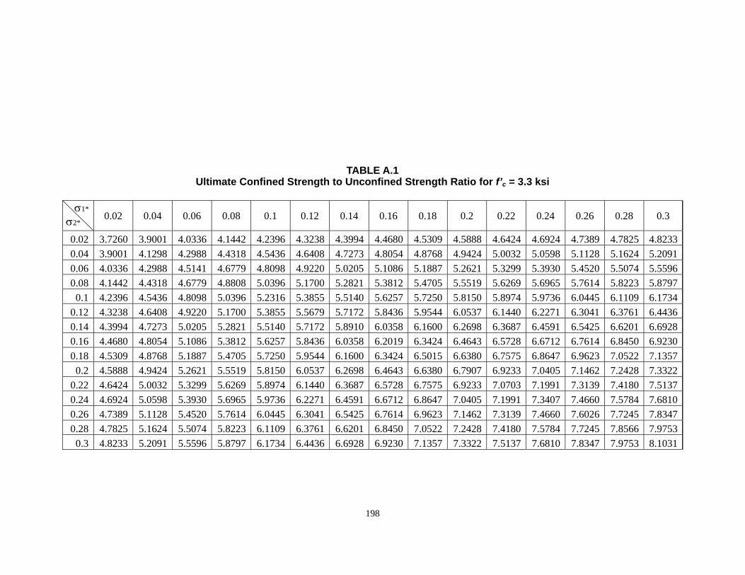
198
TABLE A.1 Ultimate Confined Strength to Unconfined Strength Ratio for f’c = 3.3 ksi
0.02 0.04 0.06 0.08 0.1 0.12 0.14 0.16 0.18 0.2 0.22 0.24 0.26 0.28 0.3
0.02 3.7260 3.9001 4.0336 4.1442 4.2396 4.3238 4.3994 4.4680 4.5309 4.5888 4.6424 4.6924 4.7389 4.7825 4.8233
0.04 3.9001 4.1298 4.2988 4.4318 4.5436 4.6408 4.7273 4.8054 4.8768 4.9424 5.0032 5.0598 5.1128 5.1624 5.2091
0.06 4.0336 4.2988 4.5141 4.6779 4.8098 4.9220 5.0205 5.1086 5.1887 5.2621 5.3299 5.3930 5.4520 5.5074 5.5596
0.08 4.1442 4.4318 4.6779 4.8808 5.0396 5.1700 5.2821 5.3812 5.4705 5.5519 5.6269 5.6965 5.7614 5.8223 5.8797
0.1 4.2396 4.5436 4.8098 5.0396 5.2316 5.3855 5.5140 5.6257 5.7250 5.8150 5.8974 5.9736 6.0445 6.1109 6.1734
0.12 4.3238 4.6408 4.9220 5.1700 5.3855 5.5679 5.7172 5.8436 5.9544 6.0537 6.1440 6.2271 6.3041 6.3761 6.4436
0.14 4.3994 4.7273 5.0205 5.2821 5.5140 5.7172 5.8910 6.0358 6.1600 6.2698 6.3687 6.4591 6.5425 6.6201 6.6928
0.16 4.4680 4.8054 5.1086 5.3812 5.6257 5.8436 6.0358 6.2019 6.3424 6.4643 6.5728 6.6712 6.7614 6.8450 6.9230
0.18 4.5309 4.8768 5.1887 5.4705 5.7250 5.9544 6.1600 6.3424 6.5015 6.6380 6.7575 6.8647 6.9623 7.0522 7.1357
0.2 4.5888 4.9424 5.2621 5.5519 5.8150 6.0537 6.2698 6.4643 6.6380 6.7907 6.9233 7.0405 7.1462 7.2428 7.3322
0.22 4.6424 5.0032 5.3299 5.6269 5.8974 6.1440 6.3687 6.5728 6.7575 6.9233 7.0703 7.1991 7.3139 7.4180 7.5137
0.24 4.6924 5.0598 5.3930 5.6965 5.9736 6.2271 6.4591 6.6712 6.8647 7.0405 7.1991 7.3407 7.4660 7.5784 7.6810
0.26 4.7389 5.1128 5.4520 5.7614 6.0445 6.3041 6.5425 6.7614 6.9623 7.1462 7.3139 7.4660 7.6026 7.7245 7.8347
0.28 4.7825 5.1624 5.5074 5.8223 6.1109 6.3761 6.6201 6.8450 7.0522 7.2428 7.4180 7.5784 7.7245 7.8566 7.9753
0.3 4.8233 5.2091 5.5596 5.8797 6.1734 6.4436 6.6928 6.9230 7.1357 7.3322 7.5137 7.6810 7.8347 7.9753 8.1031
1*
2*

199
TABLE A.2 Ultimate Confined Strength to Unconfined Strength Ratio for f’c = 3.9 ksi
0.02 0.04 0.06 0.08 0.1 0.12 0.14 0.16 0.18 0.2 0.22 0.24 0.26 0.28 0.3
0.02 4.4819 4.7318 4.9351 5.1101 5.2656 5.4063 5.5355 5.6552 5.7670 5.8721 5.9712 6.0651 6.1544 6.2394 6.3206
0.04 4.7318 5.0412 5.2854 5.4880 5.6642 5.8217 5.9649 6.0969 6.2196 6.3345 6.4427 6.5450 6.6422 6.7347 6.8230
0.06 4.9351 5.2854 5.5802 5.8187 6.0197 6.1962 6.3548 6.4998 6.6337 6.7587 6.8759 6.9865 7.0914 7.1911 7.2862
0.08 5.1101 5.4880 5.8187 6.1005 6.3333 6.5323 6.7083 6.8674 7.0134 7.1488 7.2753 7.3943 7.5068 7.6136 7.7154
0.1 5.2656 5.6642 6.0197 6.3333 6.6037 6.8308 7.0273 7.2024 7.3616 7.5081 7.6443 7.7720 7.8923 8.0062 8.1145
0.12 5.4063 5.8217 6.1962 6.5323 6.8308 7.0908 7.3125 7.5063 7.6802 7.8389 7.9855 8.1222 8.2506 8.3718 8.4868
0.14 5.5355 5.9649 6.3548 6.7083 7.0273 7.3125 7.5631 7.7795 7.9704 8.1427 8.3007 8.4471 8.5840 8.7128 8.8346
0.16 5.6552 6.0969 6.4998 6.8674 7.2024 7.5063 7.7795 8.0215 8.2328 8.4208 8.5913 8.7483 8.8942 9.0310 9.1599
0.18 5.7670 6.2196 6.6337 7.0134 7.3616 7.6802 7.9704 8.2328 8.4670 8.6733 8.8582 9.0269 9.1827 9.3279 9.4644
0.2 5.8721 6.3345 6.7587 7.1488 7.5081 7.8389 8.1427 8.4208 8.6733 8.9002 9.1018 9.2837 9.4503 9.6048 9.7492
0.22 5.9712 6.4427 6.8759 7.2753 7.6443 7.9855 8.3007 8.5913 8.8582 9.1018 9.3219 9.5190 9.6978 9.8624 10.0154
0.24 6.0651 6.5450 6.9865 7.3943 7.7720 8.1222 8.4471 8.7483 9.0269 9.2837 9.5190 9.7328 9.9255 10.1014 10.2638
0.26 6.1544 6.6422 7.0914 7.5068 7.8923 8.2506 8.5840 8.8942 9.1827 9.4503 9.6978 9.9255 10.1334 10.3220 10.4948
0.28 6.2394 6.7347 7.1911 7.6136 8.0062 8.3718 8.7128 9.0310 9.3279 9.6048 9.8624 10.1014 10.3220 10.5243 10.7080
0.3 6.3206 6.8230 7.2862 7.7154 8.1145 8.4868 8.8346 9.1599 9.4644 9.7492 10.0154 10.2638 10.4948 10.7080 10.9060
1*
2*

200
TABLE A.3 Ultimate Confined Strength to Unconfined Strength Ratio for f’c = 4.4 ksi (used by Mander et al. (1988))
0.02 0.04 0.06 0.08 0.1 0.12 0.14 0.16 0.18 0.2 0.22 0.24 0.26 0.28 0.3
0.02 5.0255 5.2550 5.4259 5.5656 5.6849 5.7895 5.8829 5.9674 6.0444 6.1152 6.1806 6.2412 6.2976 6.3502 6.3993
0.04 5.2550 5.5622 5.7791 5.9460 6.0845 6.2040 6.3096 6.4044 6.4906 6.5695 6.6423 6.7098 6.7728 6.8315 6.8866
0.06 5.4259 5.7791 6.0569 6.2623 6.4247 6.5613 6.6803 6.7860 6.8815 6.9686 7.0487 7.1230 7.1920 7.2566 7.3171
0.08 5.5656 5.9460 6.2623 6.5164 6.7112 6.8688 7.0030 7.1209 7.2263 7.3218 7.4094 7.4903 7.5654 7.6355 7.7012
0.1 5.6849 6.0845 6.4247 6.7112 6.9456 7.1307 7.2834 7.4150 7.5313 7.6359 7.7312 7.8188 7.9000 7.9756 8.0464
0.12 5.7895 6.2040 6.5613 6.8688 7.1307 7.3486 7.5248 7.6726 7.8012 7.9157 8.0193 8.1140 8.2013 8.2825 8.3582
0.14 5.8829 6.3096 6.6803 7.0030 7.2834 7.5248 7.7283 7.8964 8.0394 8.1650 8.2775 8.3797 8.4735 8.5604 8.6413
0.16 5.9674 6.4044 6.7860 7.1209 7.4150 7.6726 7.8964 8.0875 8.2480 8.3864 8.5089 8.6193 8.7200 8.8127 8.8989
0.18 6.0444 6.4906 6.8815 7.2263 7.5313 7.8012 8.0394 8.2480 8.4282 8.5818 8.7156 8.8350 8.9431 9.0422 9.1338
0.2 6.1152 6.5695 6.9686 7.3218 7.6359 7.9157 8.1650 8.3864 8.5818 8.7522 8.8994 9.0289 9.1451 9.2510 9.3483
0.22 6.1806 6.6423 7.0487 7.4094 7.7312 8.0193 8.2775 8.5089 8.7156 8.8994 9.0610 9.2022 9.3276 9.4408 9.5443
0.24 6.2412 6.7098 7.1230 7.4903 7.8188 8.1140 8.3797 8.6193 8.8350 9.0289 9.2022 9.3560 9.4916 9.6130 9.7231
0.26 6.2976 6.7728 7.1920 7.5654 7.9000 8.2013 8.4735 8.7200 8.9431 9.1451 9.3276 9.4916 9.6383 9.7687 9.8861
0.28 6.3502 6.8315 7.2566 7.6355 7.9756 8.2825 8.5604 8.8127 9.0422 9.2510 9.4408 9.6130 9.7687 9.9087 10.0343
0.3 6.3993 6.8866 7.3171 7.7012 8.0464 8.3582 8.6413 8.8989 9.1338 9.3483 9.5443 9.7231 9.8861 10.0343 10.1683
1*
2*

201
TABLE A.4 Ultimate Confined Strength to Unconfined Strength Ratio for f’c = 5.2 ksi
0.02 0.04 0.06 0.08 0.1 0.12 0.14 0.16 0.18 0.2 0.22 0.24 0.26 0.28 0.3
0.02 5.9070 6.1647 6.3409 6.4785 6.5923 6.6891 6.7730 6.8467 6.9120 6.9700 7.0217 7.0679 7.1091 7.1458 7.1783
0.04 6.1647 6.5586 6.8072 6.9847 7.1258 7.2436 7.3448 7.4332 7.5113 7.5810 7.6435 7.6996 7.7502 7.7959 7.8370
0.06 6.3409 6.8072 7.1633 7.4023 7.5789 7.7215 7.8417 7.9458 8.0373 8.1187 8.1917 8.2574 8.3170 8.3710 8.4201
0.08 6.4785 6.9847 7.4023 7.7279 7.9573 8.1317 8.2746 8.3962 8.5020 8.5957 8.6794 8.7548 8.8231 8.8853 8.9420
0.1 6.5923 7.1258 7.5789 7.9573 8.2579 8.4780 8.6495 8.7917 8.9137 9.0206 9.1157 9.2010 9.2782 9.3485 9.4126
0.12 6.6891 7.2436 7.7215 8.1317 8.4780 8.7576 8.9688 9.1369 9.2778 9.3996 9.5070 9.6028 9.6893 9.7678 9.8395
0.14 6.7730 7.3448 7.8417 8.2746 8.6495 8.9688 9.2303 9.4332 9.5975 9.7367 9.8579 9.9652 10.0615 10.1486 10.2280
0.16 6.8467 7.4332 7.9458 8.3962 8.7917 9.1369 9.4332 9.6790 9.8740 10.0344 10.1716 10.2917 10.3987 10.4951 10.5826
0.18 6.9120 7.5113 8.0373 8.5020 8.9137 9.2778 9.5975 9.8740 10.1061 10.2937 10.4501 10.5850 10.7039 10.8102 10.9063
0.2 6.9700 7.5810 8.1187 8.5957 9.0206 9.3996 9.7367 10.0344 10.2937 10.5135 10.6941 10.8465 10.9790 11.0964 11.2019
0.22 7.0217 7.6435 8.1917 8.6794 9.1157 9.5070 9.8579 10.1716 10.4501 10.6941 10.9029 11.0770 11.2255 11.3555 11.4713
0.24 7.0679 7.6996 8.2574 8.7548 9.2010 9.6028 9.9652 10.2917 10.5850 10.8465 11.0770 11.2759 11.4438 11.5885 11.7159
0.26 7.1091 7.7502 8.3170 8.8231 9.2782 9.6893 10.0615 10.3987 10.7039 10.9790 11.2255 11.4438 11.6338 11.7959 11.9367
0.28 7.1458 7.7959 8.3710 8.8853 9.3485 9.7678 10.1486 10.4951 10.8102 11.0964 11.3555 11.5885 11.7959 11.9776 12.1342
0.3 7.1783 7.8370 8.4201 8.9420 9.4126 9.8395 10.2280 10.5826 10.9063 11.2019 11.4713 11.7159 11.9367 12.1342 12.3084
1*
2*

202
TABLE A.5 Ultimate Confined Strength to Unconfined Strength Ratio for f’c = 3.3 ksi (using Scickert and Winkler (1977))
0.02 0.04 0.06 0.08 0.1 0.12 0.14 0.16 0.18 0.2 0.22 0.24 0.26 0.28 0.3
0.02 3.7369 3.9076 4.0347 4.1385 4.2272 4.3050 4.3745 4.4373 4.4946 4.5472 4.5958 4.6408 4.6827 4.7218 4.7584
0.04 3.9076 4.1360 4.2973 4.4214 4.5244 4.6133 4.6918 4.7623 4.8263 4.8850 4.9391 4.9894 5.0361 5.0799 5.1208
0.06 4.0347 4.2973 4.5039 4.6566 4.7773 4.8789 4.9674 5.0460 5.1170 5.1818 5.2414 5.2966 5.3479 5.3959 5.4410
0.08 4.1385 4.4214 4.6566 4.8456 4.9904 5.1076 5.2074 5.2950 5.3734 5.4445 5.5096 5.5697 5.6255 5.6777 5.7266
0.1 4.2272 4.5244 4.7773 4.9904 5.1647 5.3023 5.4159 5.5137 5.6002 5.6780 5.7489 5.8140 5.8744 5.9306 5.9832
0.12 4.3050 4.6133 4.8789 5.1076 5.3023 5.4643 5.5954 5.7053 5.8009 5.8861 5.9631 6.0335 6.0984 6.1588 6.2151
0.14 4.3745 4.6918 4.9674 5.2074 5.4159 5.5954 5.7467 5.8717 5.9780 6.0714 6.1551 6.2311 6.3009 6.3654 6.4256
0.16 4.4373 4.7623 5.0460 5.2950 5.5137 5.7053 5.8717 6.0138 6.1332 6.2361 6.3271 6.4092 6.4841 6.5531 6.6171
0.18 4.4946 4.8263 5.1170 5.3734 5.6002 5.8009 5.9780 6.1332 6.2671 6.3813 6.4809 6.5696 6.6500 6.7237 6.7918
0.2 4.5472 4.8850 5.1818 5.4445 5.6780 5.8861 6.0714 6.2361 6.3813 6.5081 6.6175 6.7138 6.8003 6.8789 6.9513
0.22 4.5958 4.9391 5.2414 5.5096 5.7489 5.9631 6.1551 6.3271 6.4809 6.6175 6.7377 6.8427 6.9359 7.0201 7.0970
0.24 4.6408 4.9894 5.2966 5.5697 5.8140 6.0335 6.2311 6.4092 6.5696 6.7138 6.8427 6.9571 7.0579 7.1481 7.2300
0.26 4.6827 5.0361 5.3479 5.6255 5.8744 6.0984 6.3009 6.4841 6.6500 6.8003 6.9359 7.0579 7.1669 7.2639 7.3512
0.28 4.7218 5.0799 5.3959 5.6777 5.9306 6.1588 6.3654 6.5531 6.7237 6.8789 7.0201 7.1481 7.2639 7.3681 7.4614
0.3 4.7584 5.1208 5.4410 5.7266 5.9832 6.2151 6.4256 6.6171 6.7918 6.9513 7.0970 7.2300 7.3512 7.4614 7.5611
1*
2*

203
TABLE A.6 Ultimate Confined Strength to Unconfined Strength Ratio for f’c = 3.9 ksi (Using Scickert and Winkler (1977))
0.02 0.04 0.06 0.08 0.1 0.12 0.14 0.16 0.18 0.2 0.22 0.24 0.26 0.28 0.3
0.02 4.4163 4.6181 4.7683 4.8909 4.9958 5.0877 5.1698 5.2441 5.3118 5.3740 5.4314 5.4846 5.5342 5.5804 5.6236
0.04 4.6181 4.8880 5.0786 5.2253 5.3470 5.4520 5.5448 5.6281 5.7038 5.7732 5.8372 5.8965 5.9518 6.0035 6.0519
0.06 4.7683 5.0786 5.3228 5.5032 5.6460 5.7660 5.8705 5.9635 6.0474 6.1239 6.1944 6.2596 6.3203 6.3770 6.4302
0.08 4.8909 5.2253 5.5032 5.7266 5.8977 6.0362 6.1542 6.2577 6.3504 6.4344 6.5113 6.5824 6.6484 6.7100 6.7677
0.1 4.9958 5.3470 5.6460 5.8977 6.1038 6.2664 6.4006 6.5162 6.6184 6.7104 6.7941 6.8711 6.9424 7.0089 7.0711
0.12 5.0877 5.4520 5.7660 6.0362 6.2664 6.4578 6.6127 6.7426 6.8557 6.9563 7.0473 7.1305 7.2072 7.2785 7.3452
0.14 5.1698 5.5448 5.8705 6.1542 6.4006 6.6127 6.7916 6.9392 7.0650 7.1753 7.2742 7.3640 7.4465 7.5228 7.5939
0.16 5.2441 5.6281 5.9635 6.2577 6.5162 6.7426 6.9392 7.1072 7.2483 7.3699 7.4775 7.5745 7.6630 7.7445 7.8202
0.18 5.3118 5.7038 6.0474 6.3504 6.6184 6.8557 7.0650 7.2483 7.4066 7.5416 7.6592 7.7641 7.8591 7.9462 8.0267
0.2 5.3740 5.7732 6.1239 6.4344 6.7104 6.9563 7.1753 7.3699 7.5416 7.6913 7.8207 7.9345 8.0367 8.1297 8.2152
0.22 5.4314 5.8372 6.1944 6.5113 6.7941 7.0473 7.2742 7.4775 7.6592 7.8207 7.9628 8.0868 8.1970 8.2964 8.3874
0.24 5.4846 5.8965 6.2596 6.5824 6.8711 7.1305 7.3640 7.5745 7.7641 7.9345 8.0868 8.2220 8.3412 8.4478 8.5446
0.26 5.5342 5.9518 6.3203 6.6484 6.9424 7.2072 7.4465 7.6630 7.8591 8.0367 8.1970 8.3412 8.4700 8.5846 8.6878
0.28 5.5804 6.0035 6.3770 6.7100 7.0089 7.2785 7.5228 7.7445 7.9462 8.1297 8.2964 8.4478 8.5846 8.7077 8.8175
0.3 5.6236 6.0519 6.4302 6.7677 7.0711 7.3452 7.5939 7.8202 8.0267 8.2152 8.3874 8.5446 8.6878 8.8175 8.9358
1*
2*

204
Table A.7 Ultimate Confined Strength to Unconfined Strength Ratio for f’c = 5.2 ksi (Using Scickert and Winkler (1977))
0.02 0.04 0.06 0.08 0.1 0.12 0.14 0.16 0.18 0.2 0.22 0.24 0.26 0.28 0.3
0.02 5.8885 6.1574 6.3577 6.5213 6.6610 6.7836 6.8931 6.9921 7.0823 7.1652 7.2418 7.3128 7.3788 7.4405 7.4980
0.04 6.1574 6.5173 6.7715 6.9671 7.1294 7.2694 7.3931 7.5042 7.6051 7.6976 7.7829 7.8620 7.9357 8.0046 8.0692
0.06 6.3577 6.7715 7.0970 7.3376 7.5279 7.6880 7.8274 7.9513 8.0632 8.1652 8.2592 8.3461 8.4270 8.5027 8.5736
0.08 6.5213 6.9671 7.3376 7.6354 7.8636 8.0483 8.2056 8.3437 8.4672 8.5792 8.6818 8.7765 8.8645 8.9467 9.0237
0.1 6.6610 7.1294 7.5279 7.8636 8.1384 8.3552 8.5342 8.6883 8.8246 8.9472 9.0588 9.1615 9.2566 9.3452 9.4281
0.12 6.7836 7.2694 7.6880 8.0483 8.3552 8.6105 8.8169 8.9902 9.1409 9.2750 9.3963 9.5073 9.6096 9.7047 9.7935
0.14 6.8931 7.3931 7.8274 8.2056 8.5342 8.8169 9.0554 9.2523 9.4200 9.5671 9.6989 9.8187 9.9286 10.0304 10.1251
0.16 6.9921 7.5042 7.9513 8.3437 8.6883 8.9902 9.2523 9.4763 9.6644 9.8265 9.9700 10.0994 10.2174 10.3261 10.4270
0.18 7.0823 7.6051 8.0632 8.4672 8.8246 9.1409 9.4200 9.6644 9.8755 10.0554 10.2123 10.3522 10.4789 10.5949 10.7023
0.2 7.1652 7.6976 8.1652 8.5792 8.9472 9.2750 9.5671 9.8265 10.0554 10.2551 10.4276 10.5793 10.7155 10.8396 10.9536
0.22 7.2418 7.7829 8.2592 8.6818 9.0588 9.3963 9.6989 9.9700 10.2123 10.4276 10.6170 10.7824 10.9293 11.0619 11.1832
0.24 7.3128 7.8620 8.3461 8.7765 9.1615 9.5073 9.8187 10.0994 10.3522 10.5793 10.7824 10.9627 11.1216 11.2637 11.3928
0.26 7.3788 7.9357 8.4270 8.8645 9.2566 9.6096 9.9286 10.2174 10.4789 10.7155 10.9293 11.1216 11.2934 11.4462 11.5838
0.28 7.4405 8.0046 8.5027 8.9467 9.3452 9.7047 10.0304 10.3261 10.5949 10.8396 11.0619 11.2637 11.4462 11.6103 11.7574
0.3 7.4980 8.0692 8.5736 9.0237 9.4281 9.7935 10.1251 10.4270 10.7023 10.9536 11.1832 11.3928 11.5838 11.7574 11.9144
1*
2*