LQHVL Q1RUWK$ PHULFD - UIUC RailTEC Proceedings/2017... ·...

$: LQHVL Q1RUWK$ PHULFD - UIUC RailTEC Proceedings/2017... · 'hod\3huirupdqfhri'liihuhqw7udlq7\shv8qghu &rpelqdwlrqvri6wuxfwxuhgdqg)oh[leoh2shudwlrqvrq 6lqjoh 7udfn5dlozd\/lqhvl q1ruwk$$
Delay Performance of Different Train Types Under

Combinations of Structured and Flexible Operations on

Single-Track Railway Lines in North America

Darkhan Mussanov a, 1, Nao Nishio a, C. Tyler Dick, PE a a Rail Transportation and Engineering Center (RailTEC), Department of Civil and

Environmental Engineering, University of Illinois at Urbana-Champaign

205 N Mathews Ave, Urbana, IL 61801, USA 1 E-mail: [email protected], Phone: +1 (217) 244 6063

Abstract

North American freight railroads typically operate flexible train schedules where train

dispatchers resolve train conflicts in real-time. This is in contrast to Europe, Asia, or rail

transit networks where structured train operations follow a pre-planned timetable. Under

flexible operations, trains are dispatched as needed, making it an ideal approach for low-

cost transportation of bulk commodities. Recently, North American railways have

experienced a substantial decline in demand for bulk transportation of coal. However,

demand for premium intermodal traffic that must operate on more rigid schedules has

reached record levels. To handle both types of traffic efficiently, North American railways

are faced with the challenge of operating both flexible and structured train schedules on the

same route infrastructure. This paper seeks to understand how different combinations of

scheduled and flexible trains, the amount of schedule flexibility, and train priorities impact

the performance of a single-track rail corridor. Rail Traffic Controller (RTC) simulation

software was used to simulate different operating conditions for a fixed traffic volume on a

representative rail corridor. The results suggest that efforts to reduce delay and improve

level-of-service by reducing schedule flexibility show little return until operations become

highly structured with little flexibility. Scheduled trains perform best when there are fewer

flexible trains on the route while flexible trains are relatively insensitive to traffic

composition. Assigning priority to scheduled trains causes the overall average level-of-

service to deteriorate. These general trends can help practitioners plan for operation of

different scheduled and flexible train types on the same rail corridor.

Keywords

Scheduling, flexible operations, train delay, simulation, priority

1 Introduction

North American freight rail traffic reached a peak in 2006 on the strength of heavy haul

transportation of bulk commodities and double-stack containers in international trade (FRA

(2015)). Following three years of traffic declines due to economic recession, freight rail

traffic has slowly returned to 2006 levels. However, the composition and geographic

distribution of this traffic has substantially changed. Coal traffic has declined by over 20

percent since 2006 while intermodal traffic has reached record levels (AAR (2016)).

Domestic package delivery companies have driven the growth of domestic intermodal

RailLille 2017 — 7th International Conference on Railway Operations Modelling and Analysis

MUSSANOV DARKHAN, NISHIO NAO, DICK C. TYLER

759 / 1705

traffic by contributing premium traffic that requires predictable service on precise

schedules. At the same time, there has been strong public and agency interest in expanding

commuter and regional intercity passenger rail service on these same freight corridors. Thus

many rail corridors are experiencing a transition from bulk freight trains operating on

flexible schedules to maximize efficiency and economies of scale, to premium services that

require more structured operations with fixed arrival and departure times. Although,

passenger, commuter and premium intermodal trains receive higher priority on the shared

corridors compared to bulk and manifest traffic, maintaining the schedule flexibility of bulk

freight trains while simultaneously providing the precision and level-of-service required by

passenger and intermodal trains presents a substantial operational challenge on the

predominantly single-track North American rail network.

To help increase the level-of-service of a single-track railway network with different

train types, railways may add passing sidings (passing loops), extend siding lengths, and

add double track. These actions can increase line capacity, reduce delay or allow for more

flexible operations but the infrastructure projects are capital intensive and each railroad

needs to maximize their return on infrastructure investment. Understanding the capacity and

level-of-service impact of altering the number of trains that depart precisely with the

timetable and according to flexible schedules can aid practitioners in evaluating operating

plans and potential infrastructure investments.

This paper seeks to understand how different combinations of scheduled and flexible

trains impact the performance of a single-track rail corridor. Simulation experiments were

conducted to examine how increasing the number of flexible trains within baseline traffic

of all scheduled trains alters the performance of a representative rail corridor. The results

of the experiments provide a better understanding of the fundamental relationships between

the proportion of scheduled and flexible trains, amount of schedule flexibility, and train

delay. The findings of this paper are not intended to suggest that one type of operation is

better than the other but rather to help practitioners consider the interaction of flexible and

scheduled trains in evaluating line capacity and infrastructure investment.

2 Background

Railway operations can be classified into two broad types: scheduled and flexible

(Figure 1). Under scheduled operations, all of the trains in the network depart according to

a pre-planned timetable with a fixed departure time and fixed arrival time (Figure 1a). The

timetable is constructed such that any conflicts between trains are resolved and if the same

timetable is executed each day, the same trains will meet and pass at the same locations

each day. This kind of operation is very common in passenger and transit networks and

railways in Europe and Asia. Precise operation according to a rigid timetable has also been

termed structured operation (Martland (2009)).

Under flexible operations, trains do not have a fixed timetable and depart terminals as

needed or within a range of pre-determined departure times. Most North American freight

trains are operated in this manner, with train dispatchers routing the trains and resolving

conflicts in real-time (Sogin (2013a)). Since train meets and passes occur at different

locations each day, the running time of individual trains can vary greatly. Thus flexible

trains, also referred to as unscheduled trains, exhibit both flexible departure times and

flexible running times over the route (Figure 1b and 1c). The result is that flexible trains

have variable arrival times at terminals or the ends of route segments under study.



760 / 1705

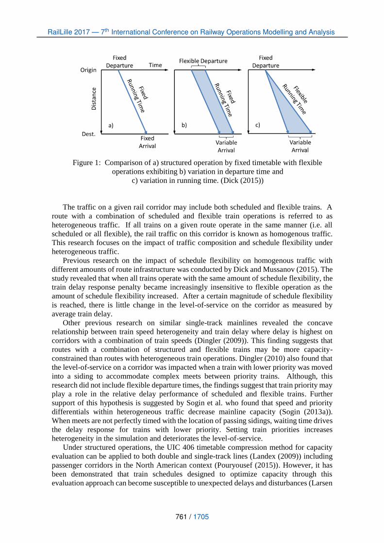
Figure 1: Comparison of a) structured operation by fixed timetable with flexible

operations exhibiting b) variation in departure time and

c) variation in running time. (Dick (2015))

The traffic on a given rail corridor may include both scheduled and flexible trains. A

route with a combination of scheduled and flexible train operations is referred to as

heterogeneous traffic. If all trains on a given route operate in the same manner (i.e. all

scheduled or all flexible), the rail traffic on this corridor is known as homogenous traffic.

This research focuses on the impact of traffic composition and schedule flexibility under

heterogeneous traffic.

Previous research on the impact of schedule flexibility on homogenous traffic with

different amounts of route infrastructure was conducted by Dick and Mussanov (2015). The

study revealed that when all trains operate with the same amount of schedule flexibility, the

train delay response penalty became increasingly insensitive to flexible operation as the

amount of schedule flexibility increased. After a certain magnitude of schedule flexibility

is reached, there is little change in the level-of-service on the corridor as measured by

average train delay.

Other previous research on similar single-track mainlines revealed the concave

relationship between train speed heterogeneity and train delay where delay is highest on

corridors with a combination of train speeds (Dingler (2009)). This finding suggests that

routes with a combination of structured and flexible trains may be more capacity-

constrained than routes with heterogeneous train operations. Dingler (2010) also found that

the level-of-service on a corridor was impacted when a train with lower priority was moved

into a siding to accommodate complex meets between priority trains. Although, this

research did not include flexible departure times, the findings suggest that train priority may

play a role in the relative delay performance of scheduled and flexible trains. Further

support of this hypothesis is suggested by Sogin et al. who found that speed and priority

differentials within heterogeneous traffic decrease mainline capacity (Sogin (2013a)).

When meets are not perfectly timed with the location of passing sidings, waiting time drives

the delay response for trains with lower priority. Setting train priorities increases

heterogeneity in the simulation and deteriorates the level-of-service.

Under structured operations, the UIC 406 timetable compression method for capacity

evaluation can be applied to both double and single-track lines (Landex (2009)) including

passenger corridors in the North American context (Pouryousef (2015)). However, it has

been demonstrated that train schedules designed to optimize capacity through this

evaluation approach can become susceptible to unexpected delays and disturbances (Larsen



761 / 1705

(2013)). Thus simulation is most often used to evaluate capacity under the flexible

operations found on most North American rail corridors (Pouryousef (2013)).

Although heterogeneity in train speed, priority and vehicle capability has been

extensively studied, these investigations did not consider the differing schedule flexibility

and level-of-service requirements of multiple types of trains. To fill this knowledge gap

and aid railway practitioners in planning operations and infrastructure, this research

investigates the behavior of routes with combinations of trains exhibiting differing amounts

of terminal departure time variability, ranging from precise schedules to complete

flexibility. This research seeks to characterize the relationship between the mixture of

scheduled and flexible trains operating on a rail corridor, the amount of schedule flexibility

in the train departure times, and the level-of-service (train delay) experienced by each type

of train.

3 Methodology

To understand the impact of dispatching two different types of railway operations on a

typical North American single-track corridor, multiple traffic scenarios were simulated on

a representative rail corridor with Rail Traffic Controller (RTC) simulation software.

3.1 Rail Traffic Controller (RTC)

RTC is an industry-leading railway simulation software commonly used by major North

American railroads and consultants to assess line capacity and aid decisions on

infrastructure investments. Unlike many other railway simulation platforms, RTC does not

require a fixed timetable with resolved train conflicts. RTC realistically models the actions

of a human train dispatcher in resolving meet and pass conflicts between trains.

RTC can also account for schedule flexibility by randomly departing trains within a

given range of departure times. For example if the schedule flexibility for a train is

specified as 60 minutes, RTC will randomly dispatch the train anytime within 60 minutes

before or after the initial set departure time during each day of the simulation. Scheduled

trains with no flexibility depart the terminal at the same exact time each day. Each

simulated day contains a different random combination of flexible train schedules along

with the trains operating on fixed schedules, resulting in differing amounts of train delay.

The train delay output is averaged over multiple days of simulated operations and

normalized by total train-miles to assess the performance of the traffic scenario.

To determine the number of simulation runs required to obtain a stable train delay

response for a given traffic scenario, an initial scenario was simulated for multiple days of

train operations and then replicated 100 times using different seeds to randomize the train

departures. Average train delay values stabilized after seven replications. Based on this

result, each traffic scenario was simulated with RTC for five days of train operations and

replicated ten times with different random seeds. The ten iterations provide 50 days of train

operations for calculation of the average train delay response associated with a given traffic

scenario in the experiment design and plotted as a single data point in the results.

3.2 Baseline Schedule and Introduction of Schedule Flexibility

For use with all of the simulation experiments, a typical North American single-track route

was constructed in RTC. The route is 386 km in length and features passing sidings that are

3.22 km long and spaced at 64 km intervals. With the exception of schedule flexibility and



762 / 1705

priority, all of the trains in the simulations have identical characteristics based on typical

North American freight trains with 115 railcars and three locomotives.

Before introducing flexible trains, a fixed baseline schedule for structured operations

was developed. The baseline schedule includes 24 trains per day that depart from either end

of the route on even intervals using a return-grid operating model on single track. In order

for all of the train meets to occur at the evenly-spaced passing sidings, the train speed,

departure interval, passing siding spacing, number of passing sidings and train

characteristics (Table 1) were carefully adjusted in RTC until delay was minimized.

Table 1: Baseline schedule parameters

Parameter Values

Length of route 386 km

Siding length 3.22 km

Siding spacing

Number of sidings

64 km

5

Traffic volume 24 trains per day

Scheduled departure

interval 2 hours

Maximum speed 37 km/hr

Locomotive type SD70 3206 kW, 3 locomotives per trainset

Train consist

Operating protocol

115 railcars at 125 tons each; 2.07 km total length

CTC 2-block, 3-aspect

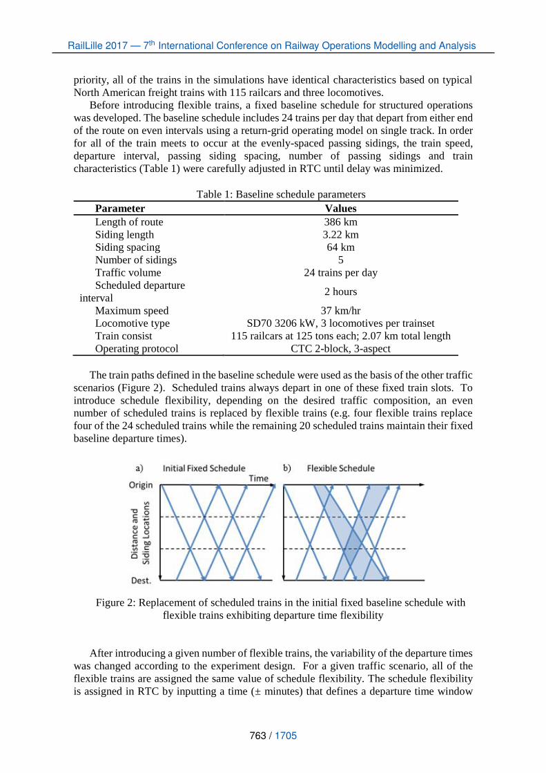
The train paths defined in the baseline schedule were used as the basis of the other traffic

scenarios (Figure 2). Scheduled trains always depart in one of these fixed train slots. To

introduce schedule flexibility, depending on the desired traffic composition, an even

number of scheduled trains is replaced by flexible trains (e.g. four flexible trains replace

four of the 24 scheduled trains while the remaining 20 scheduled trains maintain their fixed

baseline departure times).

Figure 2: Replacement of scheduled trains in the initial fixed baseline schedule with

flexible trains exhibiting departure time flexibility

After introducing a given number of flexible trains, the variability of the departure times

was changed according to the experiment design. For a given traffic scenario, all of the

flexible trains are assigned the same value of schedule flexibility. The schedule flexibility

is assigned in RTC by inputting a time (± minutes) that defines a departure time window



763 / 1705

around the corresponding departure time in the initial baseline schedule. During each

simulation day, a train will be dispatched at a random time within the departure time

window according to a uniform distribution. For this reason the headways are constantly

changing in the system. The experiment design section of this paper provides more detail

on the simulated factor levels of schedule flexibility and traffic composition.

In addition to schedule flexibility and traffic composition, another set of RTC

simulations were conducted to determine the level-of-service impact of assigning higher

priority to all of the scheduled trains.

3.3 Experiment Design and Outputs

The experiment design included three variable factors: traffic composition, schedule

flexibility and priority level. Each factor was simulated over a range of values or “levels”

(Table 2) in a full-factorial design. Simulating all factorial combinations of the factor levels

was necessary to capture the non-linear response of delay to each factor.

Table 2: Experiment Design Factors and Factor Levels

Parameter Values

Traffic Composition

(# of flexible trains out of 24 trains)

0,4, 6, 10, 12, 14, 18, 20, and 24

(% of flexible trains out of 24 trains) 0%, 17%, 25%, 58%, 50%, 58%, 75%, 83%, and

100%

Schedule Flexibility

(± minutes)

0, 10, 30, 60, 120, 180, 240, 300, 360, 420, 480,

540, 600, 660, and 720

Priority Assignment Equal Priority or

Unequal (scheduled trains have higher

priority)

Traffic composition quantifies the number of flexible trains operating on the route. This

factor can be expressed as the number of scheduled trains replaced by flexible trains per

day or as the percent of all trains on the route that operate on flexible schedules. The number

of flexible trains ranges from zero for the case of structured operations (all trains are

scheduled) to 24 for purely flexible operations (all trains are flexible). The traffic

composition factor is limited to even values to ensure an equal number of flexible trains

operate in each direction. In selecting scheduled trains to replace with flexible trains, care

is taken to evenly distribute them throughout each day (Table 3). As the traffic composition

is changed by increasing the number of flexible trains, the schedule slots taken by flexible

trains in the previous traffic compositions are maintained.

As described earlier, the schedule flexibility factor establishes the range of departure

times for each flexible train relative to the baseline schedule. The schedule flexibility factor

level of zero minutes corresponds to the structured baseline schedule with no deviation in

departure time. For higher factor levels, the departures of the flexible trains are randomized

over increasingly larger windows up to ± 720 minutes (±12 hours). At this highest factor

level, flexible trains depart each terminal randomly within each 24-hour period in a purely

unscheduled operation.

The priority assignment factor has two options that determine the relative priority of the



764 / 1705

flexible and scheduled trains. For equal priority, all scheduled and flexible trains are

assigned the same priority within RTC. For unequal priority, the scheduled trains are

assigned a higher priority value relative to flexible trains. This combination is of particular

interest since scheduled trains are likely to have higher level-of-service requirements

compared to flexible trains.

Output from the RTC simulations is reported as average train delay in minutes per 161

train-km (or 100 train-miles). This unit is very commonly used in the North American

railway industry to measure the level-of-service and define line capacity according a to a

minimum acceptable delay level. Higher delay implies congestion in the network and poor

overall performance (Sogin (2013b)). The train delay output can be calculated as an average

of all trains to assess the overall performance of the traffic scenario. The delays experienced

by scheduled and flexible trains can also be totalled separately to determine the relative

performance of each type of train.

Table 3: Replacement of scheduled trains with flexible trains (denoted by XX)

for different traffic compositions

Departure Time 0% 17% 25% 42% 50% 58% 75% 83% 100%

(0) (4) (6) (10) (12) (14) (18) (20) (24)

0:00:00 XX

2:00:00 XX XX XX XX XX XX XX XX

4:00:00 XX XX

6:00:00 XX XX XX XX XX

8:00:00 XX XX XX XX XX XX XX

10:00:00 XX XX XX

12:00:00 XX XX XX XX XX XX

14:00:00 XX XX XX

16:00:00 XX XX XX XX XX XX

18:00:00 XX XX XX XX

20:00:00 XX XX XX XX XX XX XX XX

22:00:00 XX

3.4 Types of Train Conflicts

A consequence of traffic comprised of a combination of scheduled and flexible trains is that

three different types of train meets are encountered: Scheduled – Scheduled (S-S), Flexible

– Scheduled (F-S), Flexible – Flexible (F-F). Examples of each type of conflict conflicts

can be observed in Figure 2b presented earlier in the paper. The point of intersection

between two scheduled trains (solid lines) is a S-S conflict. The F-S conflicts occur when a

scheduled train (solid line) intersects a flexible train (area). The diamond shapes in Figure

2b occur at the intersection of two flexible trains (areas) and represent a F-F conflict. The

three types of meets have different properties with respect to the range of possible meet

times and locations, and possible priority differences between the trains. These properties

influence the amount of delay that can be expected from each type of meet. The types of

train conflicts will be revisited later in the paper as a possible mechanism to explain the

simulation results.



765 / 1705

4 Results

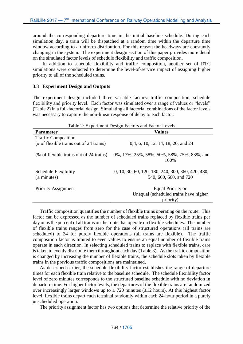
Following the completion of all simulation experiments, normalized train delay values for

each train type were plotted for the case of equal priority (Figure 3 a-b) and unequal priority

(Figure 3 c-d). The traffic composition in terms of the number of flexible trains is plotted

on the horizontal axis and the train delay response is plotted on the vertical axis. Each

coloured series displays a specific level of schedule flexibility via fitted linear or quadratic

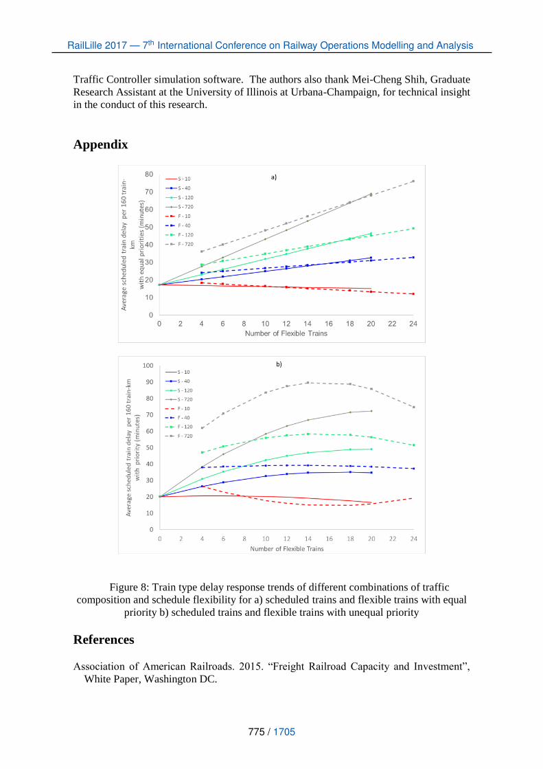
trend lines with 𝑅2 greater than 0.8. For a direct comparison of scheduled and flexible train

delay under each priority rule, see Figure 8 in the Appendix.

Figure 3: Train type delay response by traffic composition and schedule flexibility for

a) scheduled trains with equal priority b) flexible trains with equal priority c) scheduled

trains with unequal priority and d) flexible trains with unequal priority

4.1 Equal Priority

The train delay for scheduled and flexible trains with equal priority is described by a fan-

shaped set of linear relationships for each level of schedule flexibility (Figure 3a and 3b).

The linear relationships converge to a point when all the traffic is structured. As the value



766 / 1705

of schedule flexibility increases, the level-of-service deteriorates. However, there is a

greater difference in train delay between the scenarios with less schedule flexibility than the

cases with greater schedule flexibility. This follows the previous research that suggested

the delay of flexible operations increases rapidly with small amounts of schedule flexibility

but becomes insensitive to schedule flexibilities in excess of 120 minutes (Dick (2015)).

Flexible trains with schedule flexibility of 10 minutes exhibit slightly improved delay

response slightly compared to higher schedule flexibilities.

As evidenced by the linear trend in Figure 3a and 3b, for a given schedule flexibility,

each introduced flexible train adds an equal amount of average train delay, and the value of

the delay increase varies with schedule flexibility. When flexible trains are first introduced,

the flexible trains experience higher values of delay than the scheduled trains. However, as

the number of flexible trains increases, the delay response for both types of trains converges.

When there are only a small number of scheduled trains operating on a route with many

flexible trains, the delay performance of the scheduled trains is essentially indistinguishable

from the flexible trains.

A possible explanation for this last finding is that with equal priority, train conflicts do

not favor a particular type of train. If a scheduled train happens to arrive at a passing siding

earlier than a flexible train, the scheduled train will be held at the passing siding. This delay

shifts the scheduled train off the baseline schedule grid and it essentially becomes another

“flexible” train. When the number of flexible trains on the line increases, scheduled trains

encounter more F-S conflicts and therefore have a higher likelihood of transforming into a

“flexible” train that is no longer operating in its original schedule slot.

Each of the train delay trend lines in Figure 3a and 3b can be described by slope and

intercept parameters (Table 4). The intercept,𝑏(𝑆𝐹), and slope, 𝑚(𝑆𝐹), are both functions

of schedule flexibility, 𝑆𝐹. The slope term is essentially the delay contribution of each

flexible train under constant schedule flexibility. The b-intercept for scheduled trains is the

delay under the purely scheduled operation. The b-intercept for flexible trains is delay

gained from the introduction of the first 4 flexible trains. Train type delay,𝐷(𝑆𝐹, 𝑁), is

estimated as:

𝐷(𝑆𝐹, 𝑁) = 𝑚(𝑆𝐹) × 𝑁 + 𝑏(𝑆𝐹)

(1)

where,

𝑚(𝑆𝐹) = 𝐼𝑛𝑐𝑟𝑒𝑎𝑠𝑒 𝑖𝑛 𝑡𝑟𝑎𝑖𝑛 𝑑𝑒𝑙𝑎𝑦 𝑎𝑠 𝑎 𝑓𝑢𝑛𝑐𝑡𝑖𝑜𝑛 𝑜𝑓 𝑠𝑐ℎ𝑒𝑑𝑢𝑙𝑒 𝑓𝑙𝑒𝑥𝑖𝑏𝑖𝑙𝑖𝑡𝑦

𝑏(𝑆𝐹) = 𝑆𝑡𝑟𝑢𝑐𝑡𝑢𝑟𝑒𝑑 𝑜𝑝𝑒𝑟𝑎𝑡𝑖𝑜𝑛 𝑡𝑟𝑎𝑖𝑛 𝑑𝑒𝑙𝑎𝑦 𝑎𝑠 𝑎 𝑓𝑢𝑛𝑐𝑡𝑖𝑜𝑛 𝑜𝑓 𝑠𝑐ℎ𝑒𝑑𝑢𝑙𝑒 𝑓𝑙𝑒𝑥𝑖𝑏𝑖𝑙𝑖𝑡𝑦

𝑁 = 𝑁𝑢𝑚𝑏𝑒𝑟 𝑜𝑓 𝑓𝑙𝑒𝑥𝑖𝑏𝑙𝑒 𝑡𝑟𝑎𝑖𝑛𝑠 𝑖𝑛𝑡𝑟𝑜𝑑𝑢𝑐𝑒𝑑

𝑆𝐹 = 𝑆𝑐ℎ𝑒𝑑𝑢𝑙𝑒 𝑓𝑙𝑒𝑥𝑖𝑏𝑖𝑙𝑖𝑡𝑦

Table 4: Parameter estimates of train type delay for unequal priority

Train Type Slope (train/minutes) Intercept (minutes)

Scheduled trains 0.630 × ln(𝑆𝐹) − 1.56 17.3

Flexible trains 0.540 × ln (𝑆𝐹) − 1.56 2 × ln(𝑆𝐹) + 15

4.2 Unequal Priority

For the case of unequal priority, the response of scheduled train delay takes the shape of a



767 / 1705

concave function with a gradually levelling slope that becomes flat as number of flexible

trains increases (Figure 3c). The curves suggest two general ranges of interest: a low number

of flexible trains in the system (between zero and 12 flexible trains) and a high number of

flexible trains (from 12 to 24 trains). With a low number of flexible trains, train delay

continues to increase with each flexible train introduced. Replacing six scheduled trains by

flexible trains with 120 minutes of schedule flexibility nearly doubles the average train

delay. Replacing twelve scheduled trains triple the average train delay. However, after

introducing 12 flexible trains and entering the range with a high number of flexible trains,

scheduled train delay values become increasingly insensitive to the newly introduced

flexible trains.

The delay responses of flexible trains with unequal priority trace a parabolic shape

(Figure 3d). The parabola takes a concave up shape for low schedule flexibility data series

(between 0 and ± 60 minutes) and becomes concave down with high schedule flexibility

(beyond ± 60 minutes).

It is hypothesized that the overall balance between F-F, F-S and

S-S train conflict types may help explain the observed results. If the scenario does not

feature any flexible trains, only S-S meets are present minimal delay is incurred. As the

number of flexible trains is increased, a portion of the S-S conflicts are replaced by F-S and

F-F conflicts. Scenarios with more than 12 flexible trains experience a gradual replacement

of F-S and S-S meets with F-F conflicts.

When given priority, scheduled trains generally do not incur delay at F-S meets except

when meets near the end-of-route terminals. The meets near terminals often cause a

scheduled train to move off its assigned schedule slot, leading to mismatched S-S meets

further down the train path. Since the chance of terminal meet and associated delay is

proportional to the total number of F-S meets, delay for scheduled trains steadily increase

until 12 flexible trains are added.

When assigned a low priority, flexible train delay follows the concave up and down

patterns. Replacing the first four scheduled trains with flexible trains drives the average

delay of the flexible trains to be higher than scheduled trains because of F-S conflicts. As

previously mentioned, F-S conflicts are almost always resolved in favor of the higher-

priority scheduled traffic and cause substantial delay to the lower-priority flexible trains.

The delay values reach a maximum when 12 flexible trains are present. At this point there

are an equal number of scheduled and flexible trains on the route and heterogeneity in terms

of train priority and schedule is at its maximum. As the number of flexible trains increases

further, there are fewer priority scheduled trains and the likelihood of a F-S conflict

decreases while the number of F-F conflicts increase. Since both trains in a F-F conflict

have equal priority, the expected delay is shared between the flexible and scheduled trains,

and average delay begins to decrease.

Each of the train delay trend parabolas in Figure 3c and 3d can be described by a

polynomial with three parameters that are functions of schedule flexibility (Table 5). Train

type delay, 𝐷(𝑆𝐹, 𝑁), is estimated as:

𝐷(𝑆𝐹, 𝑁) = 𝑎(𝑆𝐹) × 𝑁2 + 𝑏(𝑆𝐹) × 𝑁 + 𝑐(𝑆𝐹) (2)

where,

𝑎(𝑆𝐹), 𝑏(𝑆𝐹) = 𝐼𝑛𝑐𝑟𝑒𝑎𝑠𝑒 𝑖𝑛 𝑡𝑟𝑎𝑖𝑛 𝑑𝑒𝑙𝑎𝑦 𝑎𝑠 𝑎 𝑓𝑢𝑛𝑐𝑡𝑖𝑜𝑛 𝑜𝑓 𝑠𝑐ℎ𝑒𝑑𝑢𝑙𝑒 𝑓𝑙𝑒𝑥𝑖𝑏𝑖𝑙𝑖𝑡𝑦

𝑐(𝑆𝐹) = 𝑆𝑡𝑟𝑢𝑐𝑡𝑢𝑟𝑒𝑑 𝑜𝑝𝑒𝑟𝑎𝑡𝑖𝑜𝑛 𝑡𝑟𝑎𝑖𝑛 𝑑𝑒𝑙𝑎𝑦 𝑎𝑠 𝑎 𝑓𝑢𝑛𝑐𝑡𝑖𝑜𝑛 𝑜𝑓 𝑠𝑐ℎ𝑒𝑑𝑢𝑙𝑒 𝑓𝑙𝑒𝑥𝑖𝑏𝑖𝑙𝑖𝑡𝑦

𝑁 = 𝑁𝑢𝑚𝑏𝑒𝑟 𝑜𝑓 𝑓𝑙𝑒𝑥𝑖𝑏𝑙𝑒 𝑡𝑟𝑎𝑖𝑛𝑠 𝑖𝑛𝑡𝑟𝑜𝑑𝑢𝑐𝑒𝑑

𝑆𝐹 = 𝑆𝑐ℎ𝑒𝑑𝑢𝑙𝑒 𝑓𝑙𝑒𝑥𝑖𝑏𝑖𝑙𝑖𝑡𝑦



768 / 1705

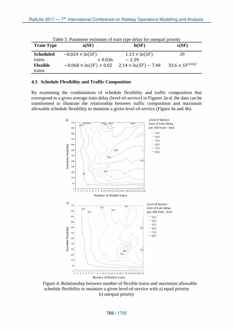
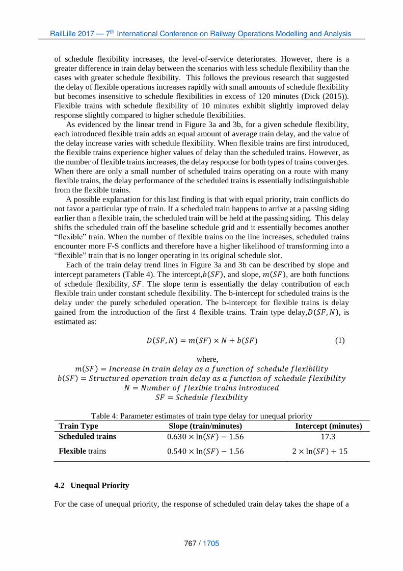
Table 5: Parameter estimates of train type delay for unequal priority

Train Type a(SF) b(SF) c(SF)

Scheduled

trains −0.024 × ln(𝑆𝐹)

+ 0.036

1.13 × ln(𝑆𝐹)− 2.39

20

Flexible

trains −0.068 × ln(𝑆𝐹) + 0.02 2.14 × ln(𝑆𝐹) − 7.48 33.6 × 𝑆𝐹0.022

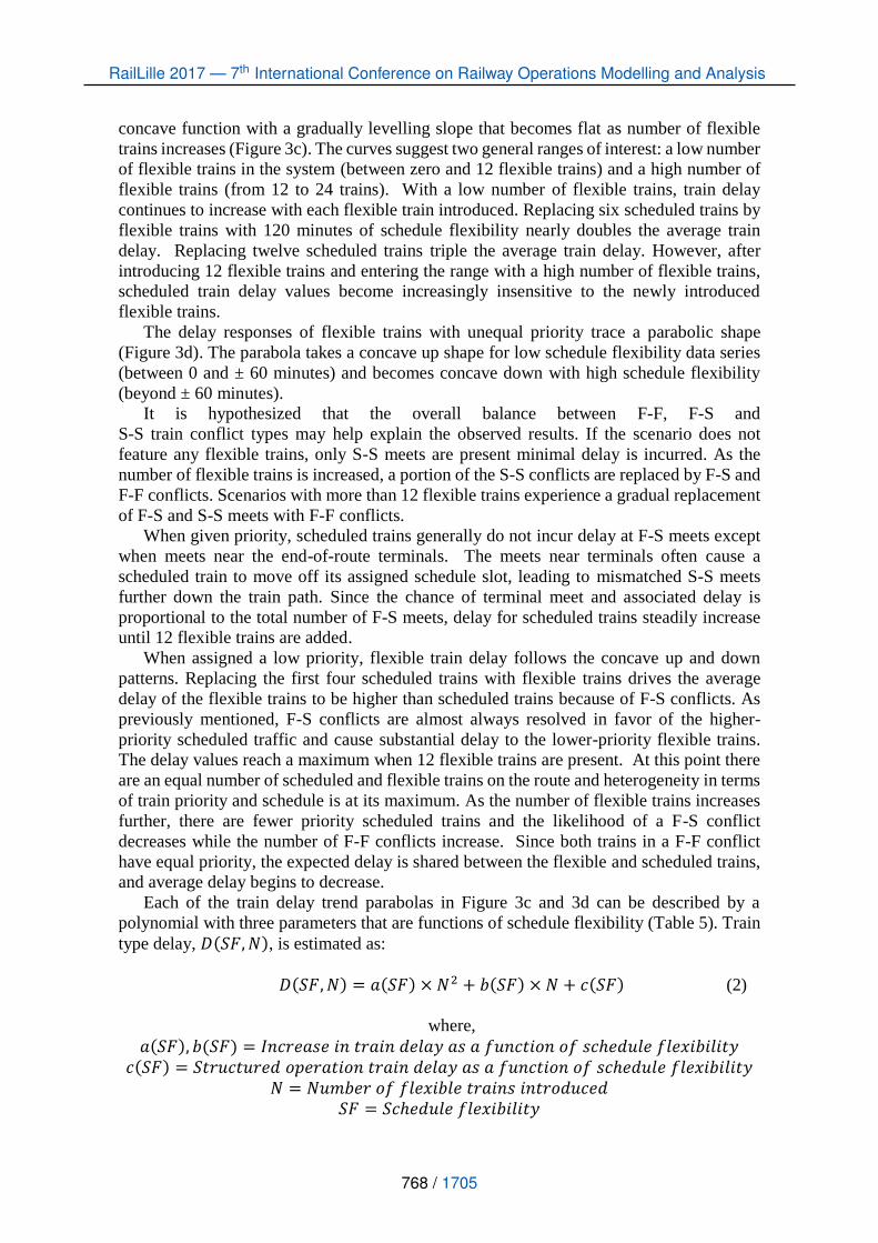
4.3 Schedule Flexibility and Traffic Composition

By examining the combinations of schedule flexibility and traffic composition that

correspond to a given average train delay (level-of-service) in Figures 3a-d, the data can be

transformed to illustrate the relationship between traffic composition and maximum

allowable schedule flexibility to maintain a given level-of-service (Figure 4a and 4b).

Figure 4: Relationship between number of flexible trains and maximum allowable

schedule flexibility to maintain a given level-of-service with a) equal priority

b) unequal priority



769 / 1705

Both figures suggest an inverse functional relationship between schedule flexibility and

number of flexible trains introduced. The amount of schedule flexibility required to

maintain the level-of-service is highly sensitive to initial increases in the number of flexible

trains. For a priority operation and a 30 minutes per 160 train-kilometres level-of-service,

the single-track route with 64 kilometre siding spacing could sustain approximately three

flexible trains with 720 minutes of scheduled flexibility. If an operator were to replace an

additional scheduled train, the schedule flexibility of all flexible trains must be reduced to

approximately to 60 minutes to maintain the desired level-of-service. To provide high levels

of schedule flexibility while maintaining a low average train delay (high level-of-service),

the number of flexible trains should be limited to three or four trains. However, if an

operator already runs flexible traffic with 60 minutes of schedule flexibility, there is an

option to convert the rest of the scheduled trains to be similarly flexible without affecting

average delay values. If majority of the trains on the line are flexible, increasing schedule

flexibility beyond 60 minutes increases delay response drastically. Overall, the results

suggest that equivalent delay performance can be obtained from the condition where there

are a small number of highly flexible trains or a large number of flexible trains with limited

schedule flexibility.

From the perspective of a capacity planner, these results suggest it is possible to

maintain a high level-of-service when a majority of the traffic is flexible by operating at

very low schedule flexibility levels. However, the level-of-service quickly deteriorates

(train delay increases) if externalities and disruptions force the operations to become more

flexible.

It is hypothesized that the delay equivalency between few but very flexible trains and

many but more structured trains arises from the ability of the flexible trains to recover to

the baseline return grid schedule train paths. Flexible trains have a certain probability to fall

close to the original return grid path and a chance to recover by meeting a scheduled train.

Trains with large amounts of schedule flexibility have a low probability to recover due to

their large range of departure times. However, flexible trains with 60 minutes of schedule

flexibility have a much higher probability of returning to their original scheduled train path.

A small number of trains with a low probability of recovery may exhibit the same delay

performance as a scenario with a large number of trains with a higher recovery probability.

5 Discussion

The following sections further expand on the presented results and suggest possible

mechanisms behind the observed trends.

5.1 Equal and Unequal Priorities

To better illustrate the effect of a change in assigned priority on the delay responses of

scheduled and flexible trains, a direct comparison is made between the train types with

equal and unequal priorities for a fixed schedule flexibility of 240 minutes (Figure 5).

When the scheduled and flexible trains are given equal priority and there are few flexible

trains, the scheduled trains have the lowest delay. As the number of flexible trains increases,

the delay of the scheduled trains converges to the same range as the flexible trains. The

scheduled trains become do disrupted by the flexible trains that the train types become

indistinguishable.



770 / 1705

When the scheduled trains are given priority, they exhibit much lower delays compared

to the lower priority flexible trains. Even as the number of flexible trains increases and

delay of both train types increases, the scheduled trains are able to take advantage of their

priority to exhibit lower delay than the flexible trains.

When the delay of scheduled trains with equal and unequal priorities is compared, the

findings are somewhat counter-intuitive. When the scheduled trains are assigned a higher

priority, their average train delay actually increases. It is hypothesized that the

disproportionate increase in train delay experienced by the flexible trains when they are

assigned a low priority effectively adds variability to train running times and the locations

of subsequent train meets, decreasing the overall performance of scheduled trains.

Figure 5: Scheduled and flexible average train delay with equal and unequal priorities for

schedule flexibility of 240 minutes

To help evaluate this hypothesis, the percent change in train delay values between the

case of equal and unequal priorities was determined for the simulated trains across all

experiment scenarios (Figure 6). Positive percent change values indicate improvement in

average train delay when priority is introduced while a negative change indicates

deterioration in average delay values. The vertical axis represents the percentage of trains

experiencing a particular percent change in delay. About 35 percent of scheduled trains do

not experience a change in performance when they are given priority.

A series Wilcoxon Rank Sum Tests was performed on the data for both scheduled and

flexible train distributions to test the null hypothesis that these two populations are identical.

The results give a p-value = 9.34 × 10−14 and at 𝛼 = 0.05, which reject the null hypothesis

stating that these populations are identical. Therefore these populations are significantly

different.

As priority is assigned to scheduled trains, the performance of flexible trains almost

always deteriorates. About 86 percent of flexible trains experience deterioration. It is

intuitive that flexible trains have higher delay values in unequal priority operation, since

train dispatcher will almost always favor a scheduled train at the conflict point. However,

the delay response of scheduled traffic is somewhat mixed. About 44 percent of scheduled



771 / 1705

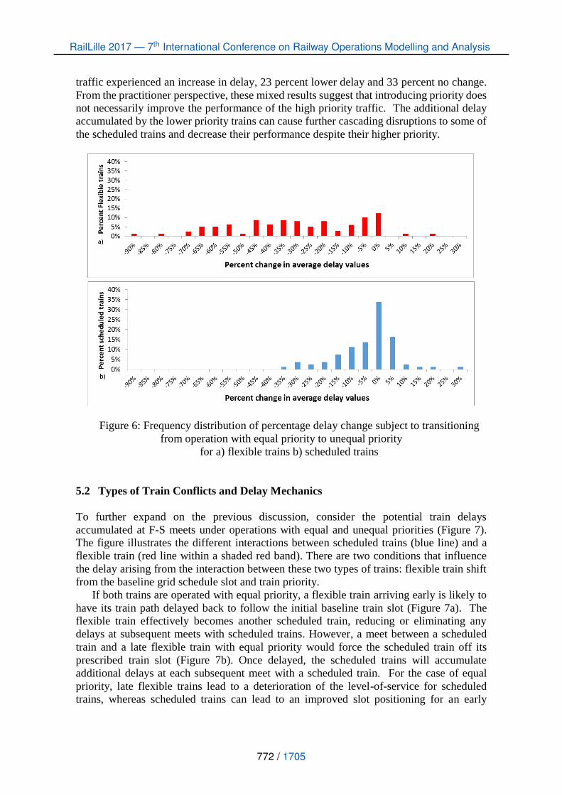
traffic experienced an increase in delay, 23 percent lower delay and 33 percent no change.

From the practitioner perspective, these mixed results suggest that introducing priority does

not necessarily improve the performance of the high priority traffic. The additional delay

accumulated by the lower priority trains can cause further cascading disruptions to some of

the scheduled trains and decrease their performance despite their higher priority.

Figure 6: Frequency distribution of percentage delay change subject to transitioning

from operation with equal priority to unequal priority

for a) flexible trains b) scheduled trains

5.2 Types of Train Conflicts and Delay Mechanics

To further expand on the previous discussion, consider the potential train delays

accumulated at F-S meets under operations with equal and unequal priorities (Figure 7).

The figure illustrates the different interactions between scheduled trains (blue line) and a

flexible train (red line within a shaded red band). There are two conditions that influence

the delay arising from the interaction between these two types of trains: flexible train shift

from the baseline grid schedule slot and train priority.

If both trains are operated with equal priority, a flexible train arriving early is likely to

have its train path delayed back to follow the initial baseline train slot (Figure 7a). The

flexible train effectively becomes another scheduled train, reducing or eliminating any

delays at subsequent meets with scheduled trains. However, a meet between a scheduled

train and a late flexible train with equal priority would force the scheduled train off its

prescribed train slot (Figure 7b). Once delayed, the scheduled trains will accumulate

additional delays at each subsequent meet with a scheduled train. For the case of equal

priority, late flexible trains lead to a deterioration of the level-of-service for scheduled

trains, whereas scheduled trains can lead to an improved slot positioning for an early



772 / 1705

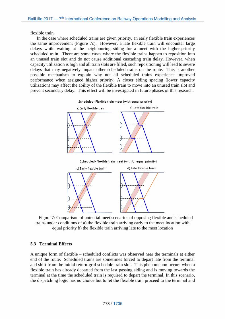
flexible train.

In the case where scheduled trains are given priority, an early flexible train experiences

the same improvement (Figure 7c). However, a late flexible train will encounter large

delays while waiting at the neighbouring siding for a meet with the higher-priority

scheduled train. There are some cases where the flexible trains happen to reposition into

an unused train slot and do not cause additional cascading train delay. However, when

capacity utilization is high and all train slots are filled, such repositioning will lead to severe

delays that may negatively impact other scheduled trains on the route. This is another

possible mechanism to explain why not all scheduled trains experience improved

performance when assigned higher priority. A closer siding spacing (lower capacity

utilization) may affect the ability of the flexible train to move into an unused train slot and

prevent secondary delay. This effect will be investigated in future phases of this research.

Figure 7: Comparison of potential meet scenarios of opposing flexible and scheduled

trains under conditions of a) the flexible train arriving early to the meet location with

equal priority b) the flexible train arriving late to the meet location

5.3 Terminal Effects

A unique form of flexible – scheduled conflicts was observed near the terminals at either

end of the route. Scheduled trains are sometimes forced to depart late from the terminal

and shift from the initial return-grid schedule train slot. This phenomenon occurs when a

flexible train has already departed from the last passing siding and is moving towards the

terminal at the time the scheduled train is required to depart the terminal. In this scenario,

the dispatching logic has no choice but to let the flexible train proceed to the terminal and



773 / 1705

delay the scheduled train even if it violates priority rules. Consequently, the scheduled train

shifts from its train slot and behaves like a flexible train with a delayed departure.

6 Conclusions and Future Work

For a given constant traffic volume and infrastructure, traffic compositions with various

levels of schedule flexibility yield distinct results depending on the assigned train priorities.

Operation with equal priorities shows little difference in performance between scheduled

and flexible trains. However, operating with unequal priorities yields distinct performance

differentials between the two train types. Delay curves with equal priorities show linear

trends for both train types; incremental introduction of flexible trains causes similar

increases in delay. Delay curves with unequal priorities display a quadratic relationship with

level-of-service being proportional to the number of flexible – scheduled (F-S) train type

conflicts. Given the infrastructure simulated in this study, operating with unequal priorities

yields mixed improvement in the performance of scheduled traffic and strict deterioration

for flexible traffic. Scheduled traffic is often delayed from its assigned departure time by

inbound flexible trains at terminals, causing the scheduled train to operate like a flexible

train and cascade secondary delay down the line.

From a level-of-service perspective, equivalent delay performance can be obtained from

the condition where there are a small number of highly flexible trains or a large number of

flexible trains each with limited schedule flexibility. From the perspective of a capacity

planner, these results suggest it is possible to maintain a high level-of-service when a

majority of the traffic is flexible by operating at very low schedule flexibility levels.

However, the level-of-service quickly deteriorates (train delay increases) if externalities and

disruptions force the operations to become more flexible.

Future work in this area will introduce various levels of infrastructure, traffic volume

and initial timetables to provide additional understanding on the trade-off between

infrastructure investment, traffic volume, schedule flexibility and initial timetable design.

For a given traffic composition and volume, a desired delay level-of-service may be

achieved through different combinations of timetable design and infrastructure investment.

Operations that isolate flexible trains to specific times of the day and wider slots could be

compensated by infrastructure investment.

As discussed above, in the case of 64 kilometre siding spacing operating with unequal

priorities yields mixed results for scheduled traffic. Operating preconditions that bring

distinct improvement to performance of scheduled traffic could provide planners with a

more refined checklist for enhancement of high priority traffic.

The number of F-F, F-S and S-S conflicts seem to govern the overall relationship

between traffic composition and schedule flexibility. Quantifying the exact impact of the

types of conflicts on the level-of-service is another logical step for future research on this

topic.

Acknowledgements

This research was supported by the National University Rail Center (NURail), a US DOT

OST Tier 1 University Transportation Center and the Association of American Railroads.

The authors thank Eric Wilson and Berkeley Simulation Software, LLC for the use of Rail



774 / 1705

Traffic Controller simulation software. The authors also thank Mei-Cheng Shih, Graduate

Research Assistant at the University of Illinois at Urbana-Champaign, for technical insight

in the conduct of this research.

Appendix

Figure 8: Train type delay response trends of different combinations of traffic

composition and schedule flexibility for a) scheduled trains and flexible trains with equal

priority b) scheduled trains and flexible trains with unequal priority

References

Association of American Railroads. 2015. “Freight Railroad Capacity and Investment”,

White Paper, Washington DC.



775 / 1705

Association of American Railroads. 2016. “Freight Railroad Capacity and Investment”,

White Paper, Washington DC.

Association of American Railroads. 2016. “Railroads and Coal”, White Paper, Washington

DC.

Dick, C.T. and D. Mussanov, 2016. “Operational schedule flexibility and infrastructure

investment: capacity trade-off on single-track railways”, Transportation Research

Record: Journal of the Transportation Research Board, 2546: 1-8.

DOI: 10.3141/2546-01.

Dingler, M.H., A. Koenig, S.L. Sogin and C.P.L. Barkan. 2010. “Determining the Causes

of Train Delay”, In: Proceedings of the Annual AREMA Conference. Orlando, FL, USA.

Dingler, M.H., Y-C. Lai and C.P.L Barkan, 2009. “Impact of train type heterogeneity on

single-track railway capacity”, Transportation Research Record: Journal of the

Transportation Research Board, 2117: 41-49.

Landex, A. 2009. “Evaluation of Railway Networks with Single Track Operation Using the

UIC 406 Capacity Method”, Netw Spat Econ,

9: 7. DOI:10.1007/s11067-008-9090-7.

Larsen, R., M. Pranzo, A. D’Ariano, F. Corman and D. Pacciarelli. 2013. “Susceptibility of

optimal train schedules to stochastic disturbances of process times”, Flexible Services

and Manufacturing Journal, 26(4): 466-489.

Martland, C.D. 2008. “Improving On-time Performance for Long-Distance Passenger

Trains Operating on Freight Routes”, Journal of the Transportation Research Forum,

Vol. 47 (Fall 2008): 63–80.

Pouryousef, H., P. Lautala and T. White. 2013. “Railroad capacity tools and methodologies

in the U.S. and Europe”, Journal of Modern Transportation,

23(1): 30-42.

Pouryousef, H., and P. Lautala. 2015. “Hybrid simulation approach for improving railway

capacity and train schedules”, Journal of Rail Transport Planning & Management, 5(4):

211-224.

Sogin, S., Y-C. Lai, C.T. Dick and C.P.L. Barkan. 2013a. “Comparison of capacity of

single- and double-track rail lines.”, Transportation Research Record: Journal of the

Transportation Research Board, 2374: 111-118.

Sogin, S. 2013b. “Simulations of mixed use rail corridors: How infrastructure affects

interactions among train types”, Master’s Thesis, University of Illinois at Urbana-

Champaign, Department of Civil and Environmental Engineering. Urbana, IL, USA.



776 / 1705

LQHVL Q1RUWK$ PHULFD - UIUC RailTEC Proceedings/2017... ·...

Documents

Transcript of LQHVL Q1RUWK$ PHULFD - UIUC RailTEC Proceedings/2017... ·...