LPV Active Power Control and Robust Analysis

for Wind Turbines

Shu Wang∗ and Peter Seiler†

Department of Aerospace Engineering & Mechanics

University of Minnesota, Minneapolis, MN, 55455, USA

Active power control (APC) refers to a mode of operation where the wind turbinetracks a desired power reference command. It enables wind farms to perform frequencyregulation and to provide ancillary services in the energy markets. This paper presents alinear parameter varying (LPV) approach for APC. The multiple-input, multiple-outputcontroller builds upon a previous gain-scheduled design. An LPV controller is designedto coordinate the blade pitch angle and generator torque, which are standard inputs toa utility scale turbine. The objective is to track a given power reference command whilealso minimizing the structural loads. The controller has parameter dependence on thewind speed and the power output. The LPV approach, in contrast to the previous ad-hoc gain scheduled design, provides (in theory) guarantees on closed-loop stability andperformance. This allows the turbine to be operated smoothly anywhere within the power/ wind speed envelope. The performance of this LPV design is evaluated using high fidelitysimulations. The robustness of the LPV system is analyzed using the theory of integralquadratic constraints.

Nomenclature

v Wind speed, m/sβ Blade pitch angle, degτ Generator torque, N ·mλ Tip speed ratio (TSR), unitlessω Rotor speed, rad/sp Generator power, MW

I. Introduction

As a promising renewable energy, wind power is increasing fast in energy markets all over the world.Though it only accounts for 3 % of the electricity produced globally in 2011, the penetration of wind energyis very high in some European countries.1 In the United States, the amount of wind energy is expected toincrease to about 30 % by 2020 to 2030.2 The power output of wind turbines is variable due to time-varyingwind speeds and this may cause unreliable operation of the power grid. This is not a significant issue whenwind power is only a small portion of the total electricity generated on the grid. However, to integrate higherlevels of variable wind power into the grid it is important for wind turbines to provide active power control(APC).3 APC can be used for the turbine to respond to fluctuations in grid frequency, termed primaryresponse, and to the power curtailment command from transmission system operator, termed secondaryresponse or automatic generation control (AGC).4

Traditional wind turbine control systems5 do not provide active power control. The power electronicsused in variable speed wind turbines decouple the mechanical/inertial turbine dynamics from the power grid.Thus a wind turbine with a traditional control law does not have the inertial response to a grid frequency

∗Graduate Student, wang2927@umn.edu†Assistant Professor, seile017@umn.edu

1 of 14

American Institute of Aeronautics and Astronautics

event like a conventional coal power generator.6 As a result the wind turbine does not participate in theprimary response. Moreover, the power output from the turbine fluctuates with variations in wind speed.As a result, new control strategies are being considered to enable wind turbines to track power commandsand possibly provide ancillary services.7–12 Some of these designs provide primary response by using inertiaresponse emulation.7,8 Another approach is to operate the wind turbine above the optimal tip speed ratiothus reserving kinetic energy.9,10 This approach enables the wind turbine to track the power commands andhence this can be used to realize AGC. The use of blade pitch control with or without combined generatortorque control has also been explored.11,12

This paper proposes an LPV controller to provide APC. The 2-input, 2-output control architecture buildsupon a previous gain-scheduled design,13 where collective blade pitch and generator torque are coordinatedin order to track power and rotor speed reference commands. The controller has parameter dependence onthe wind speed and the power output. The LPV approach, in contrast to the previous ad-hoc gain scheduleddesign, provides (in theory) guarantees on closed-loop stability and performance.14,15 This enables the LPVcontroller to have a uniform structure and operate smoothly anywhere within the power/wind speed envelopeof the turbine. It is also noted that the robustness is an important concern in modern control design forcomplex systems subject to uncertainties with the nominal model. Therefore, the robustness of this LPVsystem is analyzed using the theory of integral quadratic constraints (IQCs).16–18

The remainder of the paper is organized as follows. Section II briefly reviews the architecture for APCand the control of LPV systems. The theory of integral quadratic constraints for robust analysis of LPVsystems is in Appendix. Section III gives the detailed design process for the LPV controller. Simulationresults and robust analysis of the system are presented in Section IV. Finally, conclusions and future workare summarized in Section V.

II. Background

A. Architecture for APC

The traditional turbine control system tries to maximize power production at low wind speeds and keeprated power at high wind speeds to prevent damage of overload to the turbine.5,19,20 As shown in Figure1, the turbine using this control strategy operates on the blue curve of power versus wind speed. However,active power control requires the turbine to adjust its power output according to the command referencefrom transmission system operator or wind farm. It is important to note that the wind conditions limitthe power that can be generated (in steady-state) by the turbine. Specifically, the turbine must operatewithin the power vs. wind speed envelope below the blue curve. Thus active power control is constrained topower reference commands that are within this envelope. Methods to reserve power and operate within thisenvelope include de-rating, relative spinning reserves, and absolute spinning reserves.10,12,21 Each of thesemethods corresponds to operation along a specific power vs. wind speed curve that lies within the availablepower envelope.

Figure 1. Turbine operating regions.

An approach to realize APC has been proposed in our previous work to operate the turbine anywherewithin the power envelope.13 It enables de-rating, relative spinning reserves, and absolute spinning reservesas special cases. The control design of this approach is achieved by gain scheduling based on trim power pand wind speed v. However, the gain scheduling is less rigorous than the modern linear parameter varying(LPV) techniques.22,23 It is only sufficient for slow variations in the scheduling parameters and there are noformal guarantees on stability and performance. Therefore, a standard LPV design is applied in this paper

2 of 14

American Institute of Aeronautics and Astronautics

to achieve APC. It should be noted that LPV techniques have been applied to the control of wind turbinesin some literatures.24–26 However, these designs still try to operate the turbine in the traditional way. Abrief introduction to the control of LPV systems will be presented in Section II.B.

The way to operate the turbine to achieve APC using LPV builds upon a previous gain-scheduled design13

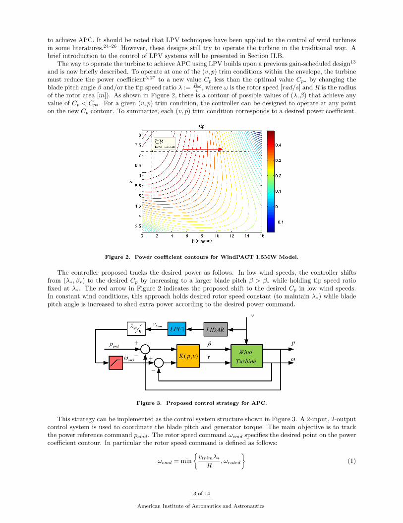
and is now briefly described. To operate at one of the (v, p) trim conditions within the envelope, the turbinemust reduce the power coefficient5,27 to a new value Cp less than the optimal value Cp∗ by changing theblade pitch angle β and/or the tip speed ratio λ := Rω

v , where ω is the rotor speed [rad/s] and R is the radiusof the rotor area [m]). As shown in Figure 2, there is a contour of possible values of (λ, β) that achieve anyvalue of Cp < Cp∗. For a given (v, p) trim condition, the controller can be designed to operate at any pointon the new Cp contour. To summarize, each (v, p) trim condition corresponds to a desired power coefficient.

Figure 2. Power coefficient contours for WindPACT 1.5MW Model.

The controller proposed tracks the desired power as follows. In low wind speeds, the controller shiftsfrom (λ∗, β∗) to the desired Cp by increasing to a larger blade pitch β > β∗ while holding tip speed ratiofixed at λ∗. The red arrow in Figure 2 indicates the proposed shift to the desired Cp in low wind speeds.In constant wind conditions, this approach holds desired rotor speed constant (to maintain λ∗) while bladepitch angle is increased to shed extra power according to the desired power command.

Figure 3. Proposed control strategy for APC.

This strategy can be implemented as the control system structure shown in Figure 3. A 2-input, 2-outputcontrol system is used to coordinate the blade pitch and generator torque. The main objective is to trackthe power reference command pcmd. The rotor speed command ωcmd specifies the desired point on the powercoefficient contour. In particular the rotor speed command is defined as follows:

ωcmd = min

{vtrimλ∗R

,ωrated

}(1)

3 of 14

American Institute of Aeronautics and Astronautics

where ωrated is the rated rotor speed and vtrim is an estimate of the effective wind speed. As describedabove, this rotor speed command attempts to keep the λ at the optimal value λ∗ at lower wind speeds. Thiswill cause an increasing rotor speed demand as wind speed increases. At higher wind speeds, the rotor speedcommand saturates and attempts to maintain the rated rotor speed. It is assumed that an accurate and realtime measurement of the wind speed is available. As shown in Figure 3, an estimate of the wind speed couldbe obtained from a LIDAR.28 Alternatively, an estimate of the effective wind speed could be constructed.29

In either case, the actual wind speed fluctuates and hence low-pass filtering, denoted LPF1 in the figure,is used to smooth out these fluctuations. As mentioned above, this LPV controller is designed to havedependence on trim wind speed vtrim and power ptrim to ensure the performance in the whole envelope. Thelow-pass filtered wind speed here also provides the corresponding scheduling parameter for the controller.The other scheduling parameter of power is from low-pass filtered power output measurement which is notshown in Figure 3.

The advantages and drawbacks of this MIMO control architecture have been discussed in.13 Comparedto the gain scheduled control, the stability can be guaranteed with a standard LPV design here, and it isexpected to achieve better performance.

B. Control of LPV Systems

LPV systems are a class of systems whose state space matrices depend on a time-varying parameter vectorρ : R+ → Rnρ . An allowable parameter trajectory ρ is a continuously differentiable function of time that isrestricted at each point in time to lie in a known compact set P ⊂ Rnρ . In addition, the parameter rates ofvariation ρ : R+ → P are assumed to lie within a hyperrectangle P defined by

P := {q ∈ Rnρ | νi ≤ qi ≤ νi, i = 1, . . . , nρ}. (2)

The set of admissible trajectories is defined as A := {ρ : R+ → Rnρ : ρ(t) ∈ P, ρ(t) ∈ P ∀t ≥ 0}. Theparameter trajectory is said to be rate unbounded if P = Rnρ .

An nthG order open loop LPV system Gρ is defined byxe

y

=

A(ρ(t)) B1(ρ(t)) B2(ρ(t))

C1(ρ(t)) D11(ρ(t)) D22(ρ(t))

C2(ρ(t)) D21(ρ(t)) D22(ρ(t))

xdu

(3)

where x ∈ RnG , d ∈ Rnd , e ∈ Rne , u ∈ Rnu and y ∈ Rny . The state-space matrices of the LPV systemare continuous functions of the parameter. Hence, LPV systems represent a special class of time-varyingsystems. Throughout the remainder of the paper the explicit dependence on t is suppressed to shorten thenotation. Moreover, it is important to emphasize that the state matrices are allowed to have an arbitrarydependence on the parameters.

The performance of an LPV system Gρ can be specified in terms of its induced L2 gain from input d tooutput e. The induced L2 norm is defined by

‖Gρ‖ := supd6=0,d∈L2,ρ∈A,x(0)=0

‖e‖‖d‖

. (4)

In words, this is the largest input/output gain over all possible inputs d ∈ L2 and allowable trajectoriesρ ∈ A.

This norm forms the basis for the induced L2 norm controller synthesis.30,31 Consider the open loopLPV system Gρ as described in Equation 3, the goal is to synthesize an LPV controller Kρ of the form:[

xK

u

]=

[AK(ρ) BK(ρ)

CK(ρ) DK(ρ)

][xK

y

]. (5)

The controller generates the control input u. It has a linear dependence on the measurement y but anarbitrary dependence on the (measurable) parameter ρ. The closed-loop interconnection of Gρ and Kρ

is given by a lower linear fractional transformation (LFT) and is denoted Fl(Gρ,Kρ). The objective is to

4 of 14

American Institute of Aeronautics and Astronautics

synthesize a controller Kρ of the specified form to minimize the closed-loop induced L2 gain from disturbancesd to errors e:

minKρ‖Fl(Gρ,Kρ)‖ . (6)

A simple, necessary and sufficient condition does not exist to evaluate the induced L2 norm of an LPVsystem. However, there are bounded-real type linear matrix inequality (LMI) conditions that are sufficient toupper bound the gain of an LPV system (Lemma 3.1 in31). This sufficient condition forms the basis for thesynthesis result.31 It should be noted that the synthesis leads to an infinite collection of parameter-dependentlinear matrix inequalities (LMIs). A remedy to this problem, which works in many practical examples, is toapproximate the set P by a finite set Pgrid ∈ P that represents a gridding over P.

III. LPV Control Design

This section provides details on the LPV approach introduced in Section II.A. The controller is designedfor the WindPACT 1.5 MW wind turbine whose model is contained in the FAST simulation package.32

First, an LPV model of the turbine is generated by selecting a gridding set of scheduling parameters thatcovers the envelope for APC and linearization at each trim point. Next, the control design and realizationis described for this grid based LPV model.

A. Model Description

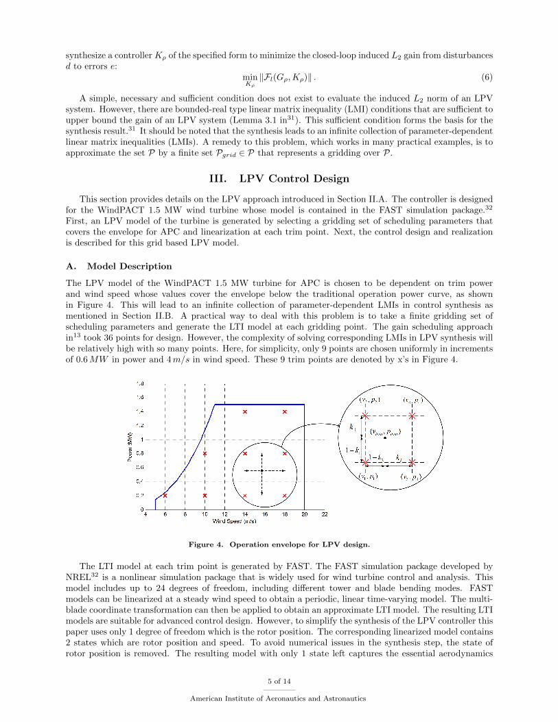
The LPV model of the WindPACT 1.5 MW turbine for APC is chosen to be dependent on trim powerand wind speed whose values cover the envelope below the traditional operation power curve, as shownin Figure 4. This will lead to an infinite collection of parameter-dependent LMIs in control synthesis asmentioned in Section II.B. A practical way to deal with this problem is to take a finite gridding set ofscheduling parameters and generate the LTI model at each gridding point. The gain scheduling approachin13 took 36 points for design. However, the complexity of solving corresponding LMIs in LPV synthesis willbe relatively high with so many points. Here, for simplicity, only 9 points are chosen uniformly in incrementsof 0.6MW in power and 4m/s in wind speed. These 9 trim points are denoted by x’s in Figure 4.

Figure 4. Operation envelope for LPV design.

The LTI model at each trim point is generated by FAST. The FAST simulation package developed byNREL32 is a nonlinear simulation package that is widely used for wind turbine control and analysis. Thismodel includes up to 24 degrees of freedom, including different tower and blade bending modes. FASTmodels can be linearized at a steady wind speed to obtain a periodic, linear time-varying model. The multi-blade coordinate transformation can then be applied to obtain an approximate LTI model. The resulting LTImodels are suitable for advanced control design. However, to simplify the synthesis of the LPV controller thispaper uses only 1 degree of freedom which is the rotor position. The corresponding linearized model contains2 states which are rotor position and speed. To avoid numerical issues in the synthesis step, the state ofrotor position is removed. The resulting model with only 1 state left captures the essential aerodynamics

5 of 14

American Institute of Aeronautics and Astronautics

and rotor dynamics of a wind turbine. This model does not contain structural dynamics but it simplifiesthe design and it is useful for understanding the effectiveness of the proposed APC strategy. Moreover,this model is only used for design but the controller is evaluated using higher fidelity simulations with moredegrees of freedom in FAST.

After the trim conditions of power p0 and wind speed v0 are selected, trim values can be found for therotor speed ω0, blade pitch angle β0 and generator torque τ0. Let ∆ be used to denote the deviation of avariable from its trim condition, e.g. ∆ω := ω − ω0 denotes the deviation of the rotor speed from the trimoperating condition. The LPV model of the turbine is given by state space expression of the form[

x

y

]=

[A(ρ) B(ρ)

C(ρ) D(ρ)

][x

u

](7)

where x := ∆ω is the state, u :=

∆β

∆τ

∆v

is the vector of inputs, y :=

[∆p

∆ω

]is the vector of outputs, and

ρ :=

[vtrim

ptrim

]is the scheduling parameter which is from low-pass filtered wind speed and power output

measurements as mentioned in Section II.A.

B. Control Synthesis and Realization

Similar to the tuning in H∞ control synthesis for LTI systems,33,34 different performance weights need tobe specified in the induced L2 control of LPV systems. The augmented system for LPV synthesis is shownin Figure 5. The seven weight functions are chosen to be the same as those used for the gain scheduleddesign.13

Two performance weights, W1(s) = 5100s+ 21

200s+ 0.021and W2(s) = 2.5

100s+ 13

200s+ 0.013are used to specify the

objectives for power and rotor speed tracking. These weights are chosen to limit the low frequency error

with less emphasis on high frequency tracking. Next, W3(s) =2.5

π

1000s+ 11

s+ 21and W4(s) =

1

2000

100s+ 14

s+ 140are two weights used to penalize the actuation of blade pitch angle and generator torque, respectively. Bothweights are chosen as high pass filters to penalize high frequency control effort. Finally, the weights W5 = 0.2,W6 = 0.4 and W7 = 1.4 are used to scale the input power command, and rotor speed command, and winddisturbance to values corresponding to 0.2MW , 0.4 rad/s and 1.4m/s, respectively. More details about theweights can be found in.13

Figure 5. Augmented system for LPV synthesis.

Besides performance weights, ranges of the parameter varying rate need to be specified before synthesis.By selecting the high-pass filtered signal of the trim wind speed vtrim, which is shown in Figure 3, themaximum wind acceleration is found to be 0.3m/s2 in the average speed of 16m/s with 5 % turbulence.However, to ensure stability of the system in high turbulence, the value is extended to 1m/s2. In practical

6 of 14

American Institute of Aeronautics and Astronautics

application of APC, the reference command of power is expected to change slowly. Therefore, 0.1MW/sis selected for the trim power varying rate. A controller can be designed for a faster rate of variation fordesired power if necessary.

The LPV controller is synthesized after solving a finite collection of LMIs. The result is expressed as a setof LTI controllers corresponding to different trim points. Realization of the LPV controller requires linearinterpolation of these LTI controllers and the trim values of blade pitch angle βtrim and generator torqueτtrim. Specifically, the four nearest “grid” trim points {vi, pi}4i=1 of the current (vtrim, ptrim) are determined

as shown in Figure 4. The fractional distance along each coordinate axis is computed as k1 =p2 − ptrimp2 − p1

and k2 =v3 − vtrimv3 − v1

. Finally, the trim blade pitch and generator torque are given by

[βtrim

τtrim

]= k2

(k1

[β1

τ1

]+ (1− k1)

[β2

τ2

])+ (1− k2)

(k1

[β3

τ3

]+ (1− k1)

[β4

τ4

])(8)

Some trim conditions near the boundary of the operating area have less than four neighboring “grid” trimpoints. For conditions with only two neighbors, the interpolation is along a single dimension. For conditionswith only three neighbors, i.e. the trim point is in a triangle with vertices of (v1, p1), (v3, p3) and (v4, p4),βtrim and τtrim are given by[

βtrim

τtrim

]= k2

(k1

[β1

τ1

]+ (1− k1)

[β3

τ3

])+ (1− k2)

(k1

[β4

τ4

]+ (1− k1)

[β3

τ3

])(9)

where k1 =ptrim − p3

p4 − p3+v3 − vtrimv3 − v1

and k2 =v3 − vtrimv3 − v1

. The state-space matrices for the controller,[Ak Bk

Ck Dk

]are interpolated in a similar fashion as those given in Equation 8 and 9.

IV. Simulations and Analysis

A. Nominal Performance in Turbulent Wind

The LPV controller designed in Section III was simulated with WindPACT 1.5 MW wind turbine modelin FAST. The control design was performed using a 1-state linearized model. However, turbine structuralmodes were included in all simulation results shown in this section. Specifically, the structural modes forsimulation include the first flap-wise blade mode for each blade and the first fore-after tower bending mode.Including the rotor position, the model has five degrees of freedom. For comparison, the gain scheduled H∞controller designed in13 was also simulated. However, only nine H∞ controllers corresponding to trim pointsin the LPV design were gain scheduled.

In the first simulation, the wind profile contains 5 % turbulence at a mean wind speed of 8m/s. Thepower command (red dash-dot line in second subplot of Figure 6) steps from 0.4MW to 0.5MW at t = 150 s,then drops to 0.3MW at t = 300 s and finally steps back to 0.4MW at t = 450 s. In this wind and powerprofile, LTI controllers at trim points of (6m/s, 0.2MW ), (10m/s, 0.2MW ) and (10m/s, 0.8MW ) wereinvolved into the linear interpolation for both the LPV and gain scheduled cases. However, the system withthe gain scheduled controller was simulated to be unstable under these conditions. A detailed post-analysisrevealed that the closed-loop with the original gain-scheduled controller was unstable, i.e. it had a pole in theright half of the complex plane. The LPV controller worked well in this case. This exception demonstratesthe stability guarantee for the standard LPV design.

To continue the comparison, the LTI controller at the trim point of (6m/s, 0.2MW ) was removed for thegain scheduled case. The results are shown in Figure 6 for the gain-scheduled controller (dash green line) andthe LPV controller (solid blue line). The subplots are, from top to bottom, the rotor speed, power capture,blade pitch, and generator torque. Since the wind speed is below rated, the rotor speed command specifiedin Equation 1 is proportional to the low-pass filtered wind speed estimate. This rotor speed command isshown as the dash-dot line in the top subplot. The rotor speed regulation for the LPV controller has smallererror than the gain scheduled one. To evaluate these errors, define the root mean square (RMS) of the rotor

7 of 14

American Institute of Aeronautics and Astronautics

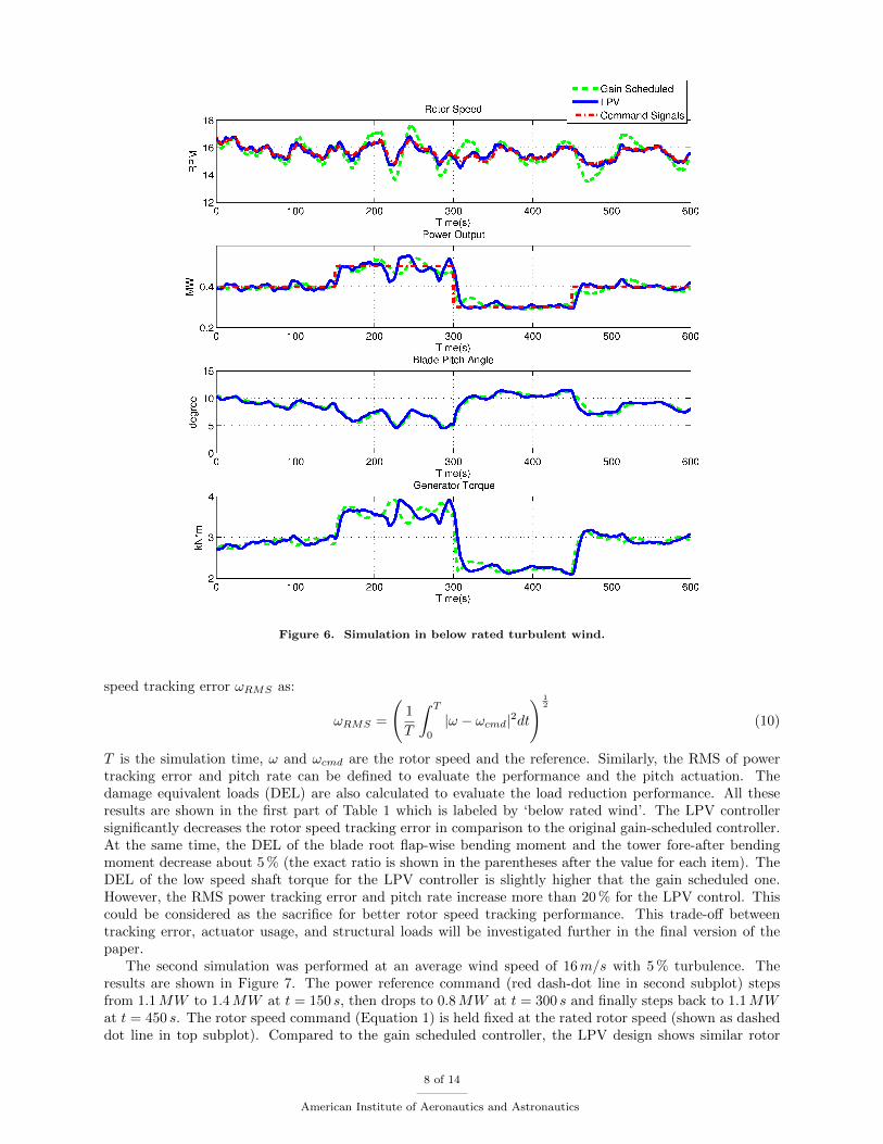
Figure 6. Simulation in below rated turbulent wind.

speed tracking error ωRMS as:

ωRMS =

(1

T

∫ T

0

|ω − ωcmd|2dt

) 12

(10)

T is the simulation time, ω and ωcmd are the rotor speed and the reference. Similarly, the RMS of powertracking error and pitch rate can be defined to evaluate the performance and the pitch actuation. Thedamage equivalent loads (DEL) are also calculated to evaluate the load reduction performance. All theseresults are shown in the first part of Table 1 which is labeled by ‘below rated wind’. The LPV controllersignificantly decreases the rotor speed tracking error in comparison to the original gain-scheduled controller.At the same time, the DEL of the blade root flap-wise bending moment and the tower fore-after bendingmoment decrease about 5 % (the exact ratio is shown in the parentheses after the value for each item). TheDEL of the low speed shaft torque for the LPV controller is slightly higher that the gain scheduled one.However, the RMS power tracking error and pitch rate increase more than 20 % for the LPV control. Thiscould be considered as the sacrifice for better rotor speed tracking performance. This trade-off betweentracking error, actuator usage, and structural loads will be investigated further in the final version of thepaper.

The second simulation was performed at an average wind speed of 16m/s with 5 % turbulence. Theresults are shown in Figure 7. The power reference command (red dash-dot line in second subplot) stepsfrom 1.1MW to 1.4MW at t = 150 s, then drops to 0.8MW at t = 300 s and finally steps back to 1.1MWat t = 450 s. The rotor speed command (Equation 1) is held fixed at the rated rotor speed (shown as dasheddot line in top subplot). Compared to the gain scheduled controller, the LPV design shows similar rotor

8 of 14

American Institute of Aeronautics and Astronautics

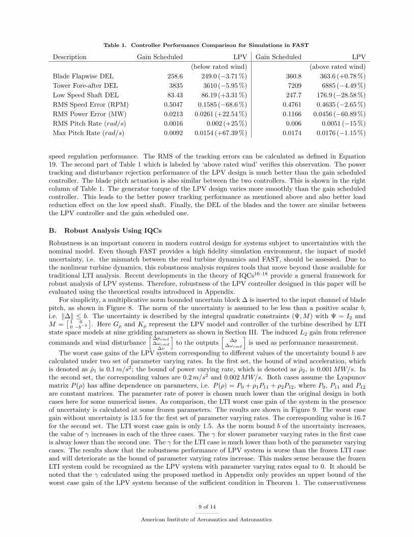
Table 1. Controller Performance Comparison for Simulations in FAST

Description Gain Scheduled LPV Gain Scheduled LPV

(below rated wind) (above rated wind)

Blade Flapwise DEL 258.6 249.0 (−3.71 %) 360.8 363.6 (+0.78 %)

Tower Fore-after DEL 3835 3610 (−5.95 %) 7209 6885 (−4.49 %)

Low Speed Shaft DEL 83.43 86.19 (+3.31 %) 247.7 176.9 (−28.58 %)

RMS Speed Error (RPM) 0.5047 0.1585 (−68.6 %) 0.4761 0.4635 (−2.65 %)

RMS Power Error (MW) 0.0213 0.0261 (+22.54 %) 0.1166 0.0456 (−60.89 %)

RMS Pitch Rate (rad/s) 0.0016 0.002 (+25 %) 0.006 0.0051 (−15 %)

Max Pitch Rate (rad/s) 0.0092 0.0154 (+67.39 %) 0.0174 0.0176 (−1.15 %)

speed regulation performance. The RMS of the tracking errors can be calculated as defined in Equation19. The second part of Table 1 which is labeled by ‘above rated wind’ verifies this observation. The powertracking and disturbance rejection performance of the LPV design is much better than the gain scheduledcontroller. The blade pitch actuation is also similar between the two controllers. This is shown in the rightcolumn of Table 1. The generator torque of the LPV design varies more smoothly than the gain scheduledcontroller. This leads to the better power tracking performance as mentioned above and also better loadreduction effect on the low speed shaft. Finally, the DEL of the blades and the tower are similar betweenthe LPV controller and the gain scheduled one.

B. Robust Analysis Using IQCs

Robustness is an important concern in modern control design for systems subject to uncertainties with thenominal model. Even though FAST provides a high fidelity simulation environment, the impact of modeluncertainty, i.e. the mismatch between the real turbine dynamics and FAST, should be assessed. Due tothe nonlinear turbine dynamics, this robustness analysis requires tools that move beyond those available fortraditional LTI analysis. Recent developments in the theory of IQCs16–18 provide a general framework forrobust analysis of LPV systems. Therefore, robustness of the LPV controller designed in this paper will beevaluated using the theoretical results introduced in Appendix.

For simplicity, a multiplicative norm bounded uncertain block ∆ is inserted to the input channel of bladepitch, as shown in Figure 8. The norm of the uncertainty is assumed to be less than a positive scalar b,i.e. ‖∆‖ ≤ b. The uncertainty is described by the integral quadratic constraints (Ψ,M) with Ψ = I2 andM =

[1 00 −b−2

]. Here Gρ and Kρ represent the LPV model and controller of the turbine described by LTI

state space models at nine gridding parameters as shown in Section III. The induced L2 gain from reference

commands and wind disturbance[ ∆pcmd

∆ωcmd∆v

]to the outputs

[∆p

∆ωcmd

]is used as performance measurement.

The worst case gains of the LPV system corresponding to different values of the uncertainty bound b arecalculated under two set of parameter varying rates. In the first set, the bound of wind acceleration, whichis denoted as ρ1 is 0.1m/s2; the bound of power varying rate, which is denoted as ρ2, is 0.001MW/s. Inthe second set, the corresponding values are 0.2m/s2 and 0.002MW/s. Both cases assume the Lyapunovmatrix P (ρ) has affine dependence on parameters, i.e. P (ρ) = P0 + ρ1P11 + ρ2P12, where P0, P11 and P12

are constant matrices. The parameter rate of power is chosen much lower than the original design in bothcases here for some numerical issues. As comparison, the LTI worst case gain of the system in the presenceof uncertainty is calculated at some frozen parameters. The results are shown in Figure 9. The worst casegain without uncertainty is 13.5 for the first set of parameter varying rates. The corresponding value is 16.7for the second set. The LTI worst case gain is only 1.5. As the norm bound b of the uncertainty increases,the value of γ increases in each of the three cases. The γ for slower parameter varying rates in the first caseis alway lower than the second one. The γ for the LTI case is much lower than both of the parameter varyingcases. The results show that the robustness performance of LPV system is worse than the frozen LTI caseand will deteriorate as the bound of parameter varying rates increase. This makes sense because the frozenLTI system could be recognized as the LPV system with parameter varying rates equal to 0. It should benoted that the γ calculated using the proposed method in Appendix only provides an upper bound of theworst case gain of the LPV system because of the sufficient condition in Theorem 1. The conservativeness

9 of 14

American Institute of Aeronautics and Astronautics

Figure 7. Simulation in above rated turbulent wind.

Figure 8. Block diagram of the LPV system with uncertainty.

of this upper bound needs to be evaluated by finding a lower bound of the worst case gain of the LPVsystem. The LTI worst case gain here provides such a lower bound. However, this lower bound is also tooconservative since it assumes zero parameter varying rates. The results provided here are preliminary. Moreinterpretations will be included in the final draft with calculation of a less conservative lower bound.

V. Conclusion

This paper proposes an LPV control design for active power control of wind turbines. The control systemarchitecture coordinates the blade pitch and the generator torque to track a power command and a specifictip speed ratio. The controller is synthesized with parameter dependence on the wind speed and the power

10 of 14

American Institute of Aeronautics and Astronautics

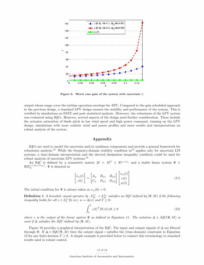
Figure 9. Worst case gain of the system with uncertain β.

output whose range cover the turbine operation envelope for APC. Compared to the gain scheduled approachin the previous design, a standard LPV design ensures the stability and performance of the system. This iscertified by simulations on FAST and post statistical analysis. Moreover, the robustness of the LPV systemwas evaluated using IQCs. However, several aspects of the design need further consideration. These includethe actuator saturation of blade pitch in low wind speed and high power command, tunning on the LPVdesign, simulations with more realistic wind and power profiles and more results and interpretations onrobust analysis of the system.

Appendix

IQCs are used to model the uncertain and/or nonlinear components and provide a general framework forrobustness analysis.16 While the frequency-domain stability condition in16 applies only for uncertain LTIsystems, a time-domain interpretation and the derived dissipation inequality condition could be used forrobust analysis of uncertain LPV systems.18

An IQC is defined by a symmetric matrix M = MT ∈ Rnz×nz and a stable linear system Ψ ∈RHnz×(nv+nw)∞ . Ψ is denoted as [

xψ(t)

z(t)

]=

[Aψ Bψ1 Bψ2

Cψ Dψ1 Dψ2

]xψ(t)

v(t)

w(t)

(11)

The initial condition for Ψ is always taken as xψ(0) = 0.

Definition 1 A bounded, causal operator ∆ : Lnv2e → Lnw2e satisfies an IQC defined by (Ψ,M) if the followinginequality holds for all v ∈ Lnv2 [0,∞), w = ∆(v) and T ≥ 0:∫ T

0

z(t)TMz(t) dt ≥ 0 (12)

where z is the output of the linear system Ψ as defined in Equation 11. The notation ∆ ∈ IQC(Ψ,M) isused if ∆ satisfies the IQC defined by (Ψ,M).

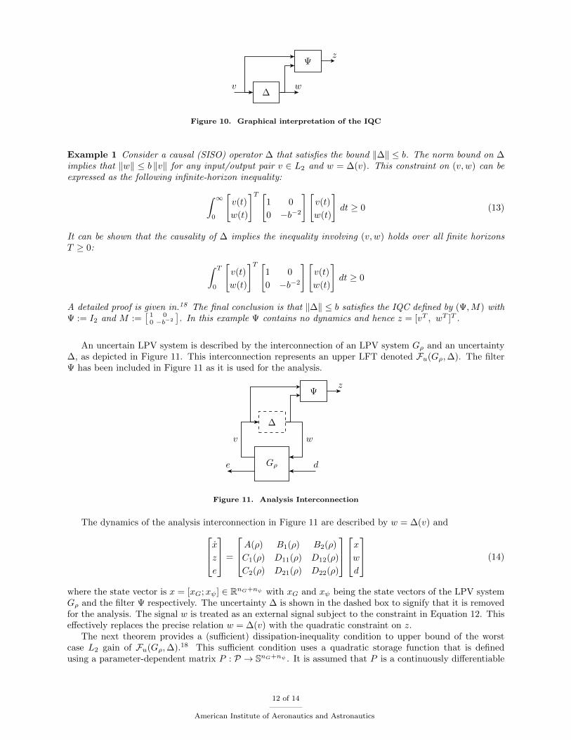
Figure 10 provides a graphical interpretation of the IQC. The input and output signals of ∆ are filteredthrough Ψ. If ∆ ∈ IQC(Ψ,M) then the output signal z satisfies the (time-domain) constraint in Equation12 for any finite-horizon T ≥ 0. A simple example is provided below to connect this terminology to standardresults used in robust control.

11 of 14

American Institute of Aeronautics and Astronautics

∆

Ψz

v w

Figure 10. Graphical interpretation of the IQC

Example 1 Consider a causal (SISO) operator ∆ that satisfies the bound ‖∆‖ ≤ b. The norm bound on ∆implies that ‖w‖ ≤ b ‖v‖ for any input/output pair v ∈ L2 and w = ∆(v). This constraint on (v, w) can beexpressed as the following infinite-horizon inequality:

∫ ∞0

[v(t)

w(t)

]T [1 0

0 −b−2

][v(t)

w(t)

]dt ≥ 0 (13)

It can be shown that the causality of ∆ implies the inequality involving (v, w) holds over all finite horizonsT ≥ 0: ∫ T

0

[v(t)

w(t)

]T [1 0

0 −b−2

][v(t)

w(t)

]dt ≥ 0

A detailed proof is given in.18 The final conclusion is that ‖∆‖ ≤ b satisfies the IQC defined by (Ψ,M) withΨ := I2 and M :=

[1 00 −b−2

]. In this example Ψ contains no dynamics and hence z = [vT , wT ]T .

An uncertain LPV system is described by the interconnection of an LPV system Gρ and an uncertainty∆, as depicted in Figure 11. This interconnection represents an upper LFT denoted Fu(Gρ,∆). The filterΨ has been included in Figure 11 as it is used for the analysis.

Gρ

∆

Ψ

de

wv

z

Figure 11. Analysis Interconnection

The dynamics of the analysis interconnection in Figure 11 are described by w = ∆(v) andxze

=

A(ρ) B1(ρ) B2(ρ)

C1(ρ) D11(ρ) D12(ρ)

C2(ρ) D21(ρ) D22(ρ)

xwd

(14)

where the state vector is x = [xG;xψ] ∈ RnG+nψ with xG and xψ being the state vectors of the LPV systemGρ and the filter Ψ respectively. The uncertainty ∆ is shown in the dashed box to signify that it is removedfor the analysis. The signal w is treated as an external signal subject to the constraint in Equation 12. Thiseffectively replaces the precise relation w = ∆(v) with the quadratic constraint on z.

The next theorem provides a (sufficient) dissipation-inequality condition to upper bound of the worstcase L2 gain of Fu(Gρ,∆).18 This sufficient condition uses a quadratic storage function that is definedusing a parameter-dependent matrix P : P → SnG+nψ . It is assumed that P is a continuously differentiable

12 of 14

American Institute of Aeronautics and Astronautics

function of the parameter ρ. In order to shorten the notation, a differential operator ∂P : P × P → SnG+nψ

is introduced as in.35 ∂P is defined as:

∂P (ρ, ρ) :=

nρ∑i=1

∂P (ρ)

∂ρiρi (15)

Theorem 1 Assume Fu(Gρ,∆) is well posed for all ∆ ∈ IQC(Ψ,M). Then the worst-case gain of Fu(Gρ,∆)is ≤ γ if there exists a continuous differentiable P ∈ P → SnG+nψ and a scalar λ ≥ 0 such that P ≥ 0 and∀(ρ, ρ) ∈ P × PPA+ATP + ∂P PB1 PB2

BT1 P 0 0

BT2 P 0 −I

+ λ

CT1DT11

DT12

M [C1 D11 D12

]+

1

γ2

CT2DT21

DT22

[C2 D21 D22

]< 0 (16)

In Equation 16 the dependence of the state matrices on ρ and ρ has been omitted.

For simplicity, details of the proof are ignored here but could be found in.18

Acknowledgments

This work was supported by the National Science Foundation under Grant No. NSF-CMMI-1254129entitled ”CAREER: Probabilistic Tools for High Reliability Monitoring and Control of Wind Farms.” Thiswork was also supported by the University of Minnesota Institute on the Environment, IREE Grants No.RS-0039-09 and RL-0011-13. Any opinions, findings, and conclusions or recommendations expressed in thismaterial are those of the authors and do not necessarily reflect the views of the National Science Foundation.

References

1“World Wind Energy Report 2011,” Proceedings of the 11 th World Energy Conference, World Wind Energy Associtation,Bonn, Germany, 2012.

2Crabtree, G., Misewich, J., Ambrosio, R., Clay, K., DeMartini, P., James, R., Lauby, M., Mohta, V., Moura, J., Sauer,P., et al., “Integrating Renewable Electricity on the Grid,” AIP Conference Proceedings-American Institute of Physics, Vol.1401, 2011, p. 387.

3Aho, J., Buckspan, A., Laks, J., Fleming, P., Jeong, Y., Dunne, F., Churchfield, M., Pao, L., and Johnson, K., “ATutorial of Wind Turbine Control for Supporting Grid Frequency through Active Power Control,” Proceedings of AmericanControl Conference, IEEE, 2012, pp. 3120–3131.

4Rebours, Y., Kirschen, D., Trotignon, M., and Rossignol, S., “A Survey of Freqency and Voltage Control AncillaryServices-Part I: Technical Features,” IEEE Transactions on Power Systems, Vol. 22, No. 1, 2007, pp. 350–357.

5Burton, T., Sharpe, D., Jenkins, N., and Bossanyi, E., Wind Energy Handbook , John Wiley & Sons, 1st ed., 2001.6Greedy, L., “Review of electrical drive-train topologies,” Project UpWind, Mekelweg, the Netherlands and Aalborg East,

Denmark, Tech. Rep, 2007.7Nelson, R. J., “Frequency-Responsive Wind Turbine Output Control,” 2011, U.S. Patent 0 001 318.8Keung, P.-K., Li, P., Banakar, H., and Ooi, B. T., “Kinetic Energy of Wind Turbine Generators for System Frequency

Support,” IEEE Transactions on Power Systems, Vol. 24, No. 1, 2009, pp. 279–287.9Juankorena, X., Esandi, I., Lopez, J., and Marroyo, L., “Method to Enable Variable Speed Wind Turbine Primary

Regulation,” International Conference on Power Engineering, Energy and Electrical Drives, 2009 , IEEE, 2009, pp. 495–500.10Aho, J., Buckspan, A., Pao, L., and Fleming, P., “An Active Power Control System for Wind Turbines Capable of

Primary and Secondary Frequency Control for Supporting Grid Reliability,” 51st AIAA Aerospace Sciences Meeting includingthe New Horizons Forum and Aerospace Exposition, 2013, pp. AIAA 2013–0456.

11Acedo Sanchez, J., Carcar, M., Lusarreta, M., Perez Barbachano, J., Simon Segura, S., Sole Lopez, D., Zabaleta Maeztu,M., Marroyo Palomo, L., Lopez Taberna, J., et al., “Method of Operation of A Wind Turbine to Guarantee Primary orSecondary Regulation in An Electric Grid,” 2011, U.S. Patent 0 057 445.

12Jeong, Y., Johnson, K., and Fleming, P., “Comparison and testing of power reserve control strategies for grid-connectedwind turbines,” Wind Energy, 2013.

13Wang, S. and Seiler, P., “Gain Scheduled Active Power Control for Wind Turbines,” AIAA Atmospheric Flight MechanicsConference, 2014.

14Apkarian, P., Gahinet, P., and Becker, G., “Self-scheduled H∞ Control of Linear Parameter-varying Systems: a DesignExamples,” Automatica, Vol. 31, No. 9, 1995, pp. 1251–1261.

15Bobanac, V., Jelavic, M., and Peric, N., “Linear Parameter Varying Approach to Wind Turbine Control,” 14th Interna-tional Power Electronics and Motion Control Conference, 2010, pp. T12–60–T12–67.

16Megretski, A. and Rantzer, A., “System Analysis via Integral Quadratic Constraints,” IEEE Trans. on AutomaticControl , Vol. 42, 1997, pp. 819–830.

13 of 14

American Institute of Aeronautics and Astronautics

17Seiler, P., “Nonlinear Stability Analysis with Dissipation Inequalities and Integral Quadratic Constraints,” Submitted tothe IEEE Trans. on Automatic Control , 2013.

18Pfifer, H. and Seiler, P., “Robustness Analysis of Linear Parameter Varying Systems Using Integral Quadratic Con-straints,” American Control Conference, 2014.

19Bossanyi, E., “The design of closed loop controllers for wind turbines,” Wind Energy, Vol. 3, 2000, pp. 149–163.20Laks, J., Pao, L., and Wright, A., “Control of Wind Turbines: Past, Present, and Future,” Proceedings of American

Control Conference, 2009, pp. 2096–2103.21Tarnowski, G., Kjær, P., Dalsgaard, S., and Nyborg, A., “Regulation and Frequency Response Service Capability of

Modern Wind Power Plants,” Proceedings of IEEE Power and Energy Society General Meeting, 2010, pp. 1–8.22Packard, A., “Gain Scheduling via Linear Fractional Transformations,” Systems and Control Letters, Vol. 22, 1994,

pp. 79–92.23Apkarian, P. and Gahinet, P., “A Convex Characterization of Gain-scheduled H∞ Controllers,” IEEE Transactions on

Automatic Control , Vol. 40, No. 5, 1995, pp. 853–864.24Bobanac, V., Jelavic, M., and Peric, N., “Linear Parameter Varying Approach to Wind Turbine Control,” 14th Interna-

tional Power Electronics and Motion Control Conference, 2010, pp. T12–60–T12–67.25Bianchi, F., Mantz, R., and Christiansen, C., “Control of variable-speed wind turbines by LPV gain scheduling,” Wind

Energy, Vol. 7, No. 1, 2004, pp. 1–8.26Bianchi, F., Mantz, R., and Christiansen, C., “Gain scheduling control of variable-speed wind energy conversion systems

using quasi-LPV models,” Control Engineering Practice, Vol. 13, No. 2, 2005, pp. 247–255.27Manwell, J., McGowan, J., and Rogers, A., Wind Energy Explained: Theory, Design, and Application, Wiley, 2010.28Mikkelsen, T., Hansen, K., Angelou, N., Sjoholm, M., Harris, M., Hadley, P., Scullion, R., Ellis, G., and Vives, G., “Lidar

wind speed measurements from a rotating spinner,” Proc. European Wind Energy Conference, Warsaw, Poland , 2010.29Knudsen, T., Bak, T., and Soltani, M., “Prediction models for wind speed at turbine locations in a wind farm,” Wind

Energy, Vol. 14, No. 7, 2011, pp. 877–894.30Wu, F., Control of Linear Parameter Varying Systems, Ph.D. thesis, University of California, Berkeley, 1995.31Wu, F., Yang, X. H., Packard, A., and Becker, G., “Induced L2 norm control for LPV systems with bounded parameter

variation rates,” International Journal of Robust and Nonlinear Control , Vol. 6, 1996, pp. 983–998.32Jonkman, J. and Buhl, M., FAST User’s Guide, National Renewable Energy Laboratory, Golden, Colorado, 2005.33Zhou, K., Doyle, J. C., and Glover, K., Robust and Optimal Control, 1st Edition, Prentice Hall, 1996.34Skogestad, S. and Postlethwaite, I., Multivariable Feedback Control , John Wiley and Sons Ltd., 2007.35Scherer, C. and Wieland, S., “Linear Matrix Inequalities in Control,” Lecture notes for a course of the dutch institute of

systems and control, Delft University of Technology, 2004.

14 of 14

American Institute of Aeronautics and Astronautics