LP-based Approximation Algorithms for Facility Location in ...

Algorithmica manuscript No.(will be inserted by the editor)

LP-based Approximation Algorithms for FacilityLocation in Buy-at-Bulk Network Design?

Zachary Friggstad · Mohsen Rezapour ·Mohammad R. Salavatipour · Jose A. Soto

Received: date / Accepted: date

Abstract We study problems that integrate buy-at-bulk network design into theclassical (connected) facility location problem. In such problems, we need to openfacilities, build a routing network, and route every client demand to an openfacility. Furthermore, capacities of the edges can be purchased in discrete unitsfrom K different cable types with costs that satisfy economies of scale.

We extend the linear programming framework of Talwar [IPCO 2002] for thesingle-source buy-at-bulk problem to these variants and prove integrality gap up-per bounds for both facility location and connected facility location buy-at-bulkproblems. For the unconnected variant we prove an integrality gap bound of O(K),and for the connected version, we get the first LP-based bound of O(1).

Keywords Buy-at-Bulk Network Design · Facility Location · ApproximationAlgorithm · LP Rounding

1 Introduction

We study problems that integrate buy-at-bulk network design into the classical(connected) facility location problem. We are interested in applications with trade-

? A preliminary version of this paper appeared in the Proceedings of the 14th InternationalSymposium on Algorithms and Data Structures (WADS) [4].

Zachary FriggstadDepartment of Computing Science, University of Alberta, Edmonton, Alberta, Canada. E-mail: [email protected]. Supported by NSERC and funding from the Canada ResearchChairs program.Mohsen RezapourDepartment of Computing Science, University of Alberta, Edmonton, Alberta, Canada. E-mail: [email protected] R. SalavatipourDepartment of Computing Science, University of Alberta, Edmonton, Alberta, Canada. E-mail: [email protected]. Supported by NSERC.Jose A. SotoDIM and CMM, Universidad de Chile, E-mail: [email protected]. Partially supported byFONDECYT grant 11130266 (Chile) and by Nucleo Milenio Informacion y Coordinacion enRedes ICM/FI P10-024F.

2 Z. Friggstad, M. Rezapour, M. Salavatipour, J. Soto

Fig. 1: An example of the fiber optic network, where red lines represent the (na-tional) core network and blue lines represent the (local) access networks.

offs between facility opening and network design costs. Problems of this type arisein the planning of optical access networks in telecommunications, for example.An operator must decide on which nodes to install routing and switching devices(these are called central offices, and represented by facilities) and on which edgesto install transmission technologies (represented by so-called cable types) to routetraffic demands. In these networks, the traffic originating from each client is sentvia tree-like access networks, to its respective facility. A combination of differentcable types may be installed on the edges of these access trees to support thetraffic flow. This allows for multiple fibers emanating from different clients toshare a single, larger cable and the same trunk on their common path towardstheir common central office. The facilities are connected amongst each other or tosome higher network level via a core network of (almost) unlimited capacity, whichis required to route the traffic further towards its destination; e.g., see Figure 1.

Designing such a network involves selecting the facilities, connecting them viahigh-bandwidth links, and dimensioning the access links that are used to routethe traffic from the clients to facilities. This can be modeled as a connected facilitylocation with buy-at-bulk edge costs problem, denoted by BBCFL. Formally, weare given a complete graph G = (V,E) with nonnegative edge lengths ce ∈ Z≥0,e ∈ E satisfying triangle inequality; a set F ⊆ V of facilities with opening costsµi ∈ Z≥0, i ∈ F ; and a set of clients D ⊆ V with demands dj ∈ Z>0, j ∈ D.We are also given K types of access cables that may be used to connect clients to

LP-based Approximation Algorithms for Buy-at-Bulk Connected Facility Location 3

Fig. 2: A feasible solution for BBCFL, where square nodes (in orange) represent(open) facilities, circle nodes in green represent clients, red lines represent corecables, and blue lines (of different thicknesses) represent access cables (of differentcapacities).

open facilities. A cable of type i has capacity ui ∈ Z>0 and cost (per unit length)σi ∈ Z≥0. Furthermore, we are given an extra type of cable, called core cable,having a cost (per unit length) of M > σK and infinite capacity, which may be usedto connect the open facilities with each other. We assume that access cable typesobey economies of scale. That is, σ1 < σ2 < · · · < σK and σ1

u1> σ2

u2> · · · > σK

uK.

A feasible solution (see Figure 2) for BBCFL consists of (1) A subset F0 ⊆ Fof facilities to open; (2) a Steiner tree of G (core network) connecting all openfacilities via core cables; and (3) a forest (access network) connecting all clientsto the open facilities. Furthermore, on each edge of this forest we have to specifya list of possibly multiple copies and types of access cables to install, in such away that the entire demand of each client can be routed along a single path toan open facility. Note that we allow the demand crossing a single edge to usedifferent access cables, but the collection of edges trasversed must be a path in G.The objective of BBCFL is to minimize the total cost of opening facilities, andconstructing core and access networks; where the cost for using edge e in the corenetwork is Mce, and the cost for installing a single copy of access cable of type ion an edge e is σice.

It is worth noting that we are allowed to install core cables on edges incidentto closed facilities, to clients, or even to nodes in V \ (F ∪ D). Nevertheless, thedemand from a client to its facility is not allowed to use core cables. The rationalityfor this constraint is that in real-life situations core and access networks are runindependently. The only way to access from the access network to the core networkis via an open facility.

There are various interesting variants of BBCFL that differ with respect to thestructure of the access or core network. For example, the planning of water andenergy supply networks occur in settings where the consideration of different con-nection types on the edges of the access network is not motivated by the differentcapacities but by the different per unit shipping cost of alternative technologiesor operational modes. This naturally leads to another interesting variant of theBBCFL problem called connected facility location with deep-discount edge costsproblem, denoted by DDCFL. In this problem, instead of capacitated access ca-bles, we are given K discount cable types, where cable type i has a fixed cost (setupcost) of σi, a flow dependent incremental cost of δi, and unbounded capacity. We


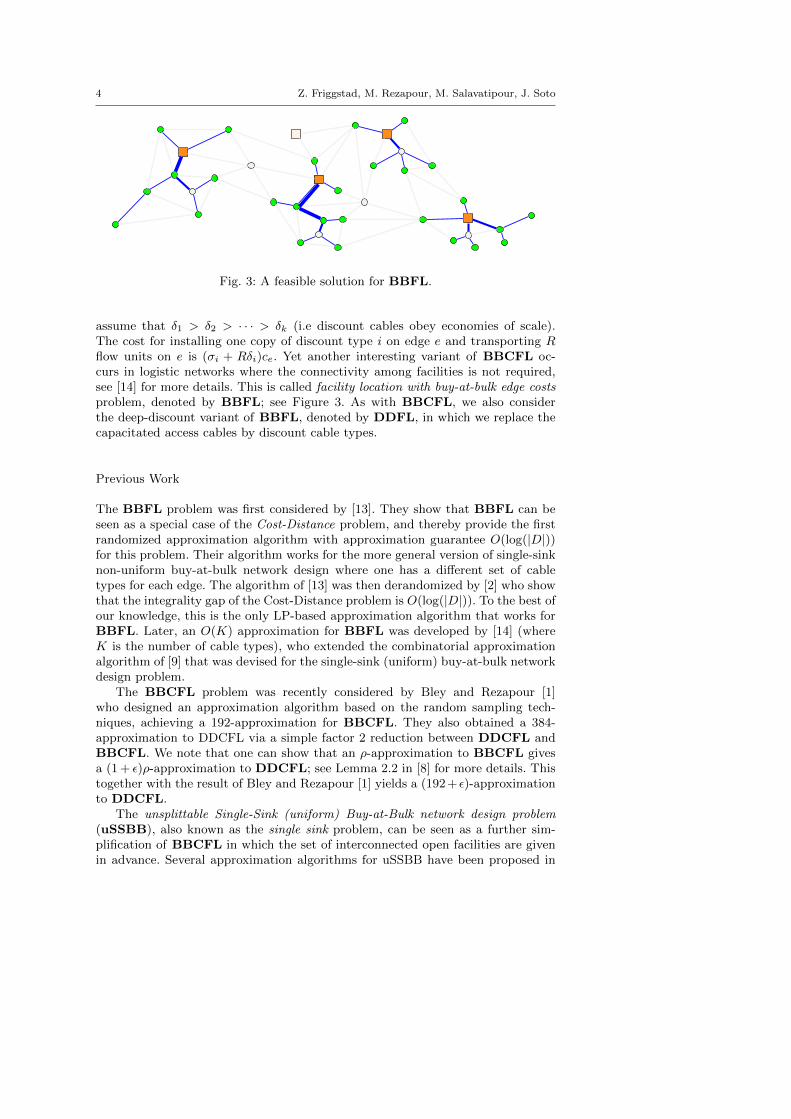
Fig. 3: A feasible solution for BBFL.

assume that δ1 > δ2 > · · · > δk (i.e discount cables obey economies of scale).The cost for installing one copy of discount type i on edge e and transporting Rflow units on e is (σi + Rδi)ce. Yet another interesting variant of BBCFL oc-curs in logistic networks where the connectivity among facilities is not required,see [14] for more details. This is called facility location with buy-at-bulk edge costsproblem, denoted by BBFL; see Figure 3. As with BBCFL, we also considerthe deep-discount variant of BBFL, denoted by DDFL, in which we replace thecapacitated access cables by discount cable types.

Previous Work

The BBFL problem was first considered by [13]. They show that BBFL can beseen as a special case of the Cost-Distance problem, and thereby provide the firstrandomized approximation algorithm with approximation guarantee O(log(|D|))for this problem. Their algorithm works for the more general version of single-sinknon-uniform buy-at-bulk network design where one has a different set of cabletypes for each edge. The algorithm of [13] was then derandomized by [2] who showthat the integrality gap of the Cost-Distance problem is O(log(|D|)). To the best ofour knowledge, this is the only LP-based approximation algorithm that works forBBFL. Later, an O(K) approximation for BBFL was developed by [14] (whereK is the number of cable types), who extended the combinatorial approximationalgorithm of [9] that was devised for the single-sink (uniform) buy-at-bulk networkdesign problem.

The BBCFL problem was recently considered by Bley and Rezapour [1]who designed an approximation algorithm based on the random sampling tech-niques, achieving a 192-approximation for BBCFL. They also obtained a 384-approximation to DDCFL via a simple factor 2 reduction between DDCFL andBBCFL. We note that one can show that an ρ-approximation to BBCFL givesa (1 + ε)ρ-approximation to DDCFL; see Lemma 2.2 in [8] for more details. Thistogether with the result of Bley and Rezapour [1] yields a (192+ ε)-approximationto DDCFL.

The unsplittable Single-Sink (uniform) Buy-at-Bulk network design problem(uSSBB), also known as the single sink problem, can be seen as a further sim-plification of BBCFL in which the set of interconnected open facilities are givenin advance. Several approximation algorithms for uSSBB have been proposed in


the literature. Using LP rounding techniques, Garg et al. [5] developed an O(K)approximation. The first constant factor approximation for this problem is dueto Guha et al. [9]. Talwar [17] showed that an LP formulation of this problemhas a constant integrality gap and provided a 216 approximation. Using samplingtechniques, this factor was reduced to 145.6 by [11], and later to 40.82 by [6].

The Connected facility location problem (ConFL) is the special case of BBCFLwith only one access cable type of unit capacity. Gupta et al. [10] obtained a 10.66-approximation for this problem, based on LP rounding. Swamy and Kumar [16]improved the approximation ratio to 8.55, using a primal-dual algorithm. Usingsampling techniques, the guarantee was later reduced to 4 by [3], and to 3.19 by[7].

Our Results

The focus of our work in this paper is on LP-based techniques. We extend theLP-based approximation for uSSBB by [17] to both buy-at-bulk facility locationand buy-at-bulk connected facility location problems and prove integrality gapupper bounds for these problems.

Similar to previous work, one can show that a ρ-approximation algorithm forDDCFL gives a 2ρ-approximation algorithm for BBCFL. For going in the otherdirection, however, there is only a factor of (1+ε) lost: ρ-approximation to BBCFLgives a (1 + ε)ρ-approximation to DDCFL; see [8] for more details.

Since the integrality gap of the natural flow-based formulation for BBCFL canbe arbitrarily large, we focus on the DDCFL problem. In Section 2, we present astrong flow-based IP, namely (IP-DDCFL), model for DDCFL. Our main resultis the following.

Theorem 1 The integrality gap of (IP-DDCFL) is at most 234.

Thus, we obtain the first LP based (deterministic) algorithm for DDCFL andthereby for BBCFL.

Using similar techniques, we finally obtain a new LP-based approximationalgorithm for the buy-at-bulk facility location problem in Section 3. We propose aflow-based IP, namely (IP-DDFL), formulation for DDFL and obtain the followingresult.

Theorem 2 The integrality gap of (IP-DDFL) is at most O(K).

This matches the approximation guarantee of the combinatorial algorithm of[14], improving the LP-based O(log(|D|))-approximation obtained by [2].

The reason why we get a better guarantee for BBCFL, even though it mayseem more difficult than BBFL, is that the extra constraints in (IP-DDCFL) thatensure connectivity among open facilities are helpful in bounding the integralitygap.

2 Buy-at-Bulk Connected Facility Location

Recall that the only difference between BBCFL and DDCFL is due to the accesscable models considered for each variant: In BBCFL, an access cable of type


k has a fixed capacity uk ∈ Z>0 and fixed setup cost σk ∈ Z≥0; whereas, inDDCFL, an access cable of type k has a setup cost σk ∈ Z≥0, a flow dependentcost of δk ∈ Z≥0, and unbounded capacity. As has been observed in the earlierworks, one can transform between buy-at-bulk and deep-discount variants of theproblem with factor 2 loss: Given an instance of BBCFL, one can consider acorresponding DDCFL instance by omitting the cable capacity uk of each accesscable k and setting its flow dependent cost to δk := σk

uk. It is not hard to see that⌈

De

uk

⌉σkce ≤

(σk +De

σk

uk

)ce ≤ 2

⌈De

uk

⌉σkce holds for any edge e, where De is the

total demand carried by edge e. Hence the total cost of the access cable installationof any solution of BBCFL is always within a factor of two of the cost of the sameaccess cable installation as the solution to the corresponding modified instance ofDDCFL, implying that an ρ-approximation to DDCFL gives a 2ρ-approximationto BBCFL.

It is not hard to show that the natural flow-based integer linear program forBBCFL has unbounded integrality gap, using the fact that an IP formulationof BBCFL has to purchase capacities in discrete unites to support the demandcarried by each edge, while the LP relaxation can pay much less for supportingthat demand by only using the last cable type, with the lowest cost per capacityratio, fractionally.

Hence in this section we focus on the DDCFL problem and get an Integralitygap of O(1) for the underlying LP of the problem, thereby obtaining a new LP-based O(1)-approximation algorithm for the BBCFL problem.

2.1 IP Modeling of DDCFL

We write a flow-based IP formulation for DDCFL. We assume w.l.o.g. that aparticular facility r is open and thus it belongs to the core network in the optimalsolution and that D ∩ F = ∅. Also, to simplify the description of our algorithm itwill be useful to add an artificial root client r∗ with unit demand, connected tor by an edge of 0 length. For each edge we create a pair of anti-parallel directedarcs, with same length as the original one. Let E be the set of these arcs. Theundirected version of an arc e ∈ E is denoted by e.

For every e ∈ E, cable type k ∈ [K] = {1, . . . ,K} and client j ∈ D, the variablef je;k indicates if flow from client j uses cable type k on arc e; for e ∈ E and k ∈ [K],

xke indicates if cable type k is installed on edge e; ze indicates if the core cable isinstalled on edge e; and yi indicates if facility i is opened.

The opening cost Cop, the core cost Ccore, the fixed cost Cfixed and the routingcost Croute of a solution are defined as

Cop =∑i∈F

µiyi; Ccore = M∑e∈E

ceze; Cfixed =K∑k=1

Cfixedk ; Croute =

K∑k=1

Croutek ,

where Cfixedk = σk

∑e∈E

cexke , and Croute

k = δk∑j∈D

dj∑e∈E

cefje;k, (1)

represent the fixed cost and routing cost of the cables of type k, respectively.We use the notation δ+(S) = {(u, v) ∈ E : u ∈ S, v /∈ S}, δ−(S) = δ+(V \ S),

δ(S) = {uv ∈ E : u ∈ S, v 6∈ S} for each S ⊆ V and δ+(v) = δ+({v}) for each


v ∈ V . Given a set of cables I ⊆ [K] and a client j ∈ D, we define the access flowon e ∈ E with respect to I and j as f je;I =

∑k∈I f

je;k; and the net in-flow on a

vertex v ∈ V with respect to I and j, as gjI(v) =∑e∈δ−(v) f

je;I −

∑e∈δ+(v) f

je;I .

We also define hji = max{gj[K](i), 0} for j ∈ D and i ∈ F . Formally, this quantityindicates whether facility i is serving client j.

With all the notation above, our integer program formulation is as follows.

min Cop + Ccore+Cfixed + Croute (IP-DDCFL)

gj[K](j) ≤ −1 ∀j ∈ D (2)

gj[K](v) = 0 ∀j ∈ D, v ∈ V \ (F ∪ {j}) (3)

gj[K](i) ≤ hji ∀j ∈ D, i ∈ F (4)

hji ≤ yi ∀j ∈ D, i ∈ F (5)

f j(u,v);k + f j(v,u);k ≤ xkuv ∀j ∈ D, k ∈ [K], uv ∈ E (6)∑

i∈S∩Fhji −

∑e∈δ(S)

ze ≤ 0 ∀j ∈ D,S ⊆ V \ {r} : S ∩ F 6= ∅ (7)

yr = 1 (8)

gj[q,K](v) ≤ 0 ∀j ∈ D, v ∈ V \ F, 1 ≤ q ≤ K (9)

gj[q,K](i)−∑e∈δ(i)

ze ≤ 0 ∀j ∈ D, i ∈ F \ {r}, 1 ≤ q ≤ K (10)

xke , fje;k, yi, ze, h

ji ∈ {0, 1} (11)

Constraints (2) impose that at least one unit of flow leaves the clients. Constraints(3) are flow conservation constraints at non-facility nodes. Constraints (4) and (5)state that the flow only terminates at open facilities. Constraints (6) ensure thatwe install access links to support the flow. Finally, Constraints (7) state that ifi is the facility serving demand j (the only i for which hji = 1) then for eachset S containing i and not containing the root there is a core link connectingS with its complement. In other words, all open facilities are connected to theroot via core links, where Constraint (8) defines the root facility. Constraints (9)and (10), called path monotonicity constraints, strengthen the linear relaxation of(IP-DDCFL). They ensure that the cable types along any path used to connectclients to facilities are nondecreasing from each client to its facility. We addressthe validity of these constraints below. Similar to that in [5], we can assume thatthe flow aggregated on an edge (in the optimum solution) never splits: once theflow from two clients share an edge they share the same set of edges on their pathsto their facility. Consider any routing path connecting client j to some facility i.As the flow never splits, the flow aggregated on edges of the path from j to i isnondecreasing. Therefore, as the access cable types obey economies of scale, wecan conclude that the cable types along any routing path (in the optimal solution)are nondecreasing from each client to its facility.

The introduction of variables hji may seem artificial, however, in the Appendixwe show that they are needed to achieve a constant integrality gap IP.


We remark that the interesting variables of this IP formulation are (f, x, y, z) =((f je;k), (xke), (yi), (ze)). All the other quantities are written in terms of these vari-ables.

2.2 Proof of Theorem 1

Let (LP-DDCFL) be the linear program relaxation of (IP-DDCFL) and (f, x, y, z)be an optimal solution to (LP-DDCFL). It is not hard to show that (LP-DDCFL)can be solved in polynomial time using, for example, the ellipsoid method. Weshow how to round this LP solution to an integer one at constant factor loss.

2.2.1 Rounding Algorithm.

We extend the rounding approach of [17] for the single-source buy-at-bulk problemto devise a rounding algorithm for DDCFL. Our algorithm has four phases.

Preprocessing Phase:

Pruning: We prune the set of access cable types such that all cables are consider-ably different. Similar to [17], this can be done without increasing the cost of theoptimal solution too much.

Theorem 3 Given ε1, ε2 ∈ (0, 1), we can prune the set of access cables so that forany i, σi+1 > σi/ε1 and δi+1 < ε2 · δi hold, increasing the installation and rout-ing costs of the optimal fractional solution by a factor of at most 1/ε1 and 1/ε2,respectively.

For the sake of notation, let [K] be the set of cables left and let (f, x, y, z) be thenew solution of (LP-DDCFL) after the pruning stage. For each client j and positiveradius R, define B(j, R) = {v ∈ V : cjv ≤ R} to be the moat centered at j. We saythat two moats B1 = B(j1, R1) and B2 = B(j2, R2) overlap if cj1j2 ≤ R1 + R2.Define also Ljk =

∑e∈E f

je;kce which represents the estimated distance that the

flow of client j travels on cables of type k. Note that Croutek = δk

∑j∈D djL

jk.

Flow path decomposition: Every client j sends (at least) one unit of flow from itselfto open facilities, specified by the f je,[K] variables. We decompose this fractionalflow into a set of paths Pj , with path p ∈ Pj starting from j and ending at somefacility. Let φ(p) denote the amount of flow of path p.

Filtering: For a predefined constant θ ∈ (0, 1) and for all j ∈ D, choose a subsetof paths Pj ⊆ Pj such that φj :=

∑p∈Pj

φ(p) ≥ θ, by selecting paths in increasing

order of their lengths until their total φ(p)-value is at least θ. For each j ∈ D,let βj be the length of the longest path in Pj . Define a new solution (f , x, y, z) asfollows. For each client j ∈ D, scale the amount of flow sent across each P ∈ Pjby 1/φj and set the flow sent across each P ∈ Pj − Pj to 0. The new flow f (andhence h) is derived naturally from this new path decomposition. For each cablek ∈ [K] and edge e ∈ E, define xke as xke/θ if there exists some j with f je′;k > 0,

where e′ ∈ E is one of the two arcs associated to e; and 0 otherwise. For each i,


set yi = min{yi/θ, 1}. And finally for each e ∈ E, set ze = min{ze/θ, 1}. It is easyto show that this solution is feasible for (LP-1).

Two important points: first, the solution (f , x, y, z) is such that the entiredemand of client j is satisfied by open facilities on the moat B(j, βj). The second

property is the following bound which is useful for the analysis. Let Pj ⊆ Pj be

the set of paths with lengths at least βj . Then, Pj includes all paths in Pj \ Pjand at least one path, say p∗ (the longest) of Pj . We conclude that

∑p∈Pj

φ(p) ≥∑p∈Pj

φ(p)−∑p∈Pj\{p∗} φ(p) ≥ 1− θ, and so

K∑k=1

Ljk =∑p∈Pj

∑e∈p

φ(p)ce ≥∑p∈Pj

φ(p)∑e∈p

ce ≥ βj(1− θ). (12)

Facility Selection Phase:

Moat selection: For a predefined constant η > 1, we consider the set of moatsBη = {B(j, ηβj) : j ∈ D} around clients. We choose a maximal set B′ ⊆ Bη ofmoats which do not overlap. We do this by processing the moats in Bη in increasingorder of their radii, and greedily adding them to B′ so that for each pair of selectedmoats in B′ with centers j, j′ ∈ D, B(j, ηβj) and B(j′, ηβj′) do not overlap. LetScore be the set of clients with moats in B′. Observe that for the artificial rootclient r∗, we have βr∗ = 0 and so r∗ ∈ Score.

Facility opening: For each j ∈ Score, let Fj = {i : hji > 0} be the facilities frac-tionally serving demand from j with respect to solution (f , x, y, z). By the firstproperty noted at the end of the preprocessing phase, Fj ⊆ B(j, ηβj), hence{Fj : j ∈ Score} consist of disjoint sets. On each Fj we open the facility ij withlowest opening cost. In particular, the root r is opened since Fr∗ = {r}. Let Ibe the set of facilities opened on this stage. The basic idea of this part of thealgorithm is inspired by [15].

For the purpose of analysis, associate each client with a special facility denotedas its (K + 1)-st proxy. Formally, for each j ∈ Score we set proxyK+1(j) = ij . Forthe remaining clients j ∈ D \ Score, we set proxyK+1(j) = proxyK+1(j′), wherej′ ∈ Score is the center of the smallest moat in B′ that overlapped with B(j, ηβj).Since the moats in B′ were added in increasing radii and (12), we get

c(j, proxyK+1(j)) ≤ (1 + 2η)βj ≤(1 + 2η)

(1− θ)

K∑q=1

Ljq ∀j ∈ D. (13)

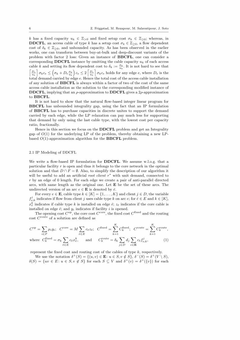
Core Network Phase: Consider the graphGK+1 obtained fromG by contractingthe nodes of each Fj into single nodes, for j ∈ Score. We construct an approximatelyoptimal Steiner tree T ′ in GK+1 having the contracted nodes as terminals. To dothis, we find an approximate Steiner tree whose cost is within a factor 2 of thecut-based relaxation. The edges of T ′ form a forest in G which touches a subsetof the facilities in Fj , called Fj , which may not include the open facility ij ; seeFigure 4(a). In order to connect all the open facilities together, we augment T ′

with the stars Qj = {ji : i ∈ Fj ∪ {ij}}, j ∈ Score; see Figure 4(b). Let T core bethe resulting tree, after possibly canceling some cycles. To conclude this stage, weinstall core cables on T core.


j2j1

j4

j3

r

(a)

j2j1

j4

j3

r

(b)

Fig. 4: An illustration of the core network installation phase on a simple instancewhere Score = {r∗, j1, j2, j4}.

Access Network Phase: We construct the access network in a top-down manner,installing cables progressively in stages numbered from i = K to 1. Let TK+1 bea minimum spanning tree on the graph induced by the set I of open facilities, andconnect them using an artificial cable type K + 1. This tree won’t appear in theend, as it will be replaced by the core network. In stage i, we augment the currenttree Ti+1, which uses only cables of type i+1 or higher, by installing cables of typei. Define Ljk to be

∑e∈E f

je;k ·ce. This estimates the distance that flow from j goes

on cable type k. Let Rjl =∑l−1k=1 L

jk be the estimated distance beyond which the

flow from j uses cable type l or higher in the new fractional solution. Intuitively,Rjl tells us how far from j to go before the LP solution installs access cable typesl or higher. Stage i consists of two steps:

Step 1. Moat Selection: For predefined γ > ζ > 1, we construct the set ofmoats Biγ = {B(j, γRji ) : j ∈ D} around all clients. We define Si to be the set of

clients whose moats intersect Ti+1. For each j ∈ Si remove moat B(j, γRji ) fromBiγ . Similar to what we did for the core network, we choose a maximal set Bi ⊆ Biγof moats which do not overlap by selecting moats from Biγ in increasing order oftheir radii. Let Si be the set of clients whose moats are selected in round i.

Step 2. Cable type i installation: We construct the set Biζ = {B(j, ζRji ) : j ∈ Si}of moats around clients in Si. We obtain a graph Gi from G by contracting eachmoat in Biζ into a super-node, and the current tree Ti+1 into a super-node called

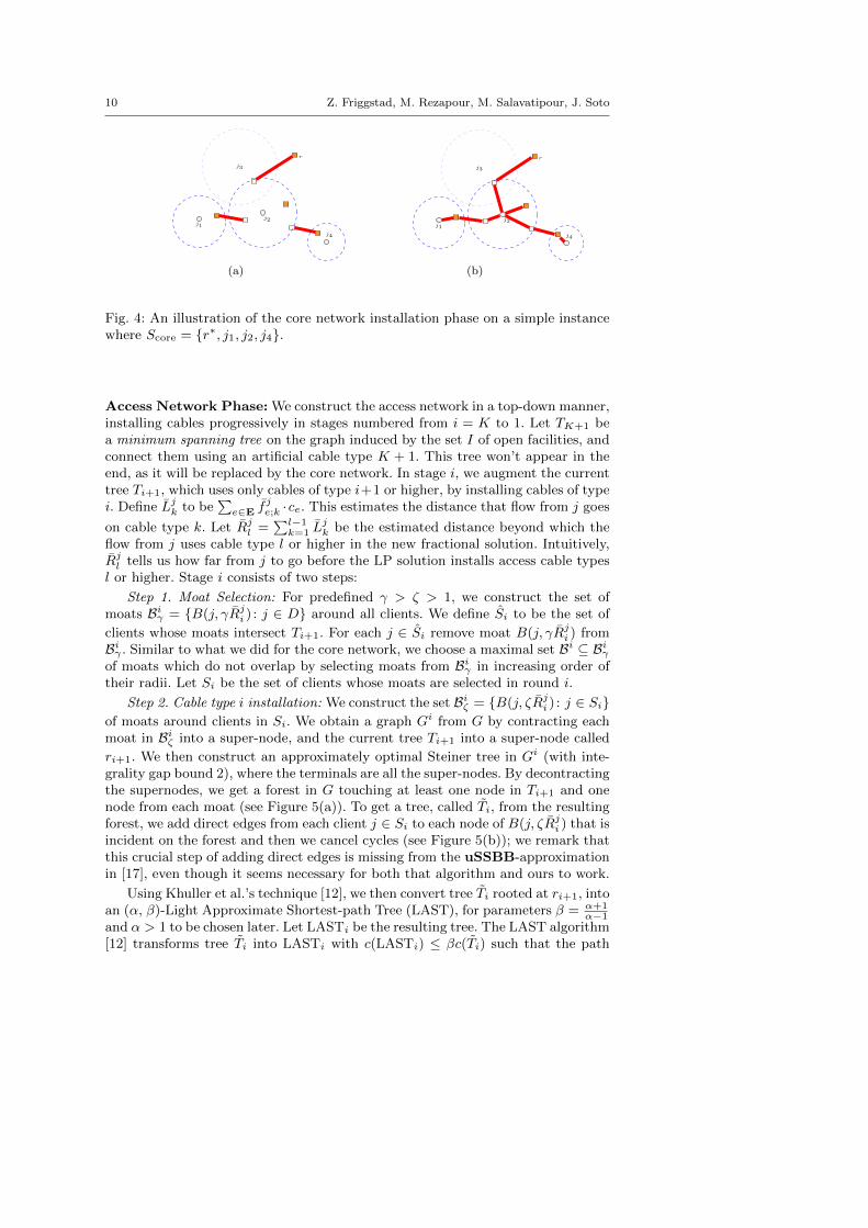
ri+1. We then construct an approximately optimal Steiner tree in Gi (with inte-grality gap bound 2), where the terminals are all the super-nodes. By decontractingthe supernodes, we get a forest in G touching at least one node in Ti+1 and onenode from each moat (see Figure 5(a)). To get a tree, called Ti, from the resultingforest, we add direct edges from each client j ∈ Si to each node of B(j, ζRji ) that isincident on the forest and then we cancel cycles (see Figure 5(b)); we remark thatthis crucial step of adding direct edges is missing from the uSSBB-approximationin [17], even though it seems necessary for both that algorithm and ours to work.

Using Khuller et al.’s technique [12], we then convert tree Ti rooted at ri+1, intoan (α, β)-Light Approximate Shortest-path Tree (LAST), for parameters β = α+1

α−1and α > 1 to be chosen later. Let LASTi be the resulting tree. The LAST algorithm[12] transforms tree Ti into LASTi with c(LASTi) ≤ βc(Ti) such that the path


j2

j3

j1

j4

j5

r

j4

(a)

j2

j3

j1

j5

r

j4

(b)

Fig. 5: An illustration of the access network phase where i = K.

length of any vertex v to root ri+1 in LASTi is at most α times the length of ashortest v-ri+1 path in Gi. We decontract the moats and install cables of type ion the edges of LASTi. Let Ti = Ti+1 ∪ LASTi.

For the purpose of analysis, for each j ∈ Si, we call an arbitrary node in its moatwhich is connected to LASTi as the proxy, denoted by proxyi(j). For the clientsj ∈ Si, we define proxyi(j) to be an arbitrary node in B(j, γRji ) ∩ Ti+1. For the

remaining clients j′ ∈ D\Si∪Si, we define proxyi(j′) to be proxyi(j), where j ∈ Si

is the center of the smallest moat in Bi that overlapped with B(j′, γRj′

i ). It is easy

to verify that c(j, proxyi(j)) ≤ 3γRji ≤3γθ

∑i−1k=1 L

jk. If we set∆ = max{1+2η

1−θ ,3γθ },

then by the previous inequality and (13), we get

c(j, proxyi+1(j)) ≤ ∆ ·i∑

q=1

Ljq, ∀j ∈ D, 1 ≤ i ≤ K (14)

which will be useful in bounding the routing cost.Finally, note that Rj1 = 0 for all j. This means that in the first step of the last

stage, S1 consists of all clients that have not been connected to the current tree.Therefore, at the end of the last stage, T1 is a tree spanning all clients and openfacilities. The access network we return consists of the forest obtained by removingthe artificial tree TK+1 from T1.

2.2.2 Analysis.

Let C∗op, C∗core, C∗fixed, and C∗route be the opening cost, core installation cost,fixed installation cost, and routing cost paid by the LP optimum, respectively (see(1)). And let Cop, Ccore, Cfixed, and Croute be the ones paid by our algorithm. LetgapST denote the upper bound on the integrality gap of the cut based formulationof Steiner tree problem, which is 2. Let OPT be the cost of LP optimum. Thefollowing lemma bounds the opening cost.

Lemma 1 The opening cost of the returned solution is at most 1θC∗op.

Proof The cost of facility ij can be bounded by using (2)-(5), and the fact that ijwas chosen as the cheapest facility of Fj ⊆ B(j, βj), as follows

µij = µij ·1

φj

∑p∈Pj

φ(p) =1

φj

∑i∈Fj

µijhji ≤

1

θ

∑i∈Fj

µiyi.


As sets Fj , j ∈ Score are disjoint, the total opening cost is at most 1θ ·∑i∈F yiµi =

1θC∗op. ut

Lemma 2 The cost of core link installation is at most η+1θ(η−1) · gapST · C∗core.

Proof By (7), one can verify that∑e∈δ+(S) ze ≥ 1 holds for any arbitrary set

S ⊂ V that contains all facilities in Fj (for some j) and it does not contain r. Thismeans that z is a feasible fractional solution to the cut based LP relaxation ofthe Steiner tree problem on the graph GK+1 (see the core network phase) whoseterminals are all the contracted sets Fj (recall that Fr∗ = {r}). In particular, theSteiner tree T ′ found in the core network phase has cost at most gapST ·

∑e∈E ceze.

The cost of the extra edges included in the final tree T core (i.e., the union of allstars Qj) can be charged to the cost of T ′ as follows.

For each facility ij in Fj let p(ij) be any path in T ′ connecting ij (which isinside B(j, βj)) to a node v outside B(j, ηβj), we note that the length of p(ij) is atleast (η− 1)βj . By a similar argument, if p(ij) = p(ik) where ij ∈ Fj and ik ∈ Fk,then we can use the fact that B(j, ηβj) and B(k, ηβk) do not overlap to concludethat the length of the path connecting ij to ik in T ′ is at least (η − 1)(βj + βk).Therefore, the total cost of the union of all Qj is at most∑

j∈Score

(c(jij) +

∑ij∈Fj

c(jij)

)≤ 2

∑j∈Score

∑ij∈Fj

βj ≤ 2∑e∈T ′

c(e)

η − 1.

Summing up, the cost of T core is at most 1 + 2(η−1) times the cost of T ′, and

therefore it is at most η+1θ(η−1) · gapST ·

∑e∈E ceze. ut

In the following, extending the ideas from [17] for uSSBB, we bound the fixedcost and routing cost of the cables installed at stage i of the access network phaseof our algorithm, denoted by Cfixed

i and Croutei , respectively.

Lemma 3 Cfixedi ≤ σi · gapST ·

γβζ

(γ − ζ)(ζ − 1)θ

( K∑q=i

1

σqC∗fixedq +

1

MC∗core

).

Proof Let S be an arbitrary subset of V \ {r} that contains B(j, ζRji ) and let

bjq;S :=∑e∈δ+(S) f

je,q denote the amount of flow from j that crosses the boundary

of S via cables of type q. We note that the flow we are considering may travelfrom j to the boundary of S using any cables of type q or less than q (due to thepath monotonicity constraints) but it must use cables of type q while crossing theboundary of S.

In the following we first show that∑i−1q=1 b

jq;S ≤

1ζ . Consider some q < i. As bjq;S

travels a distance of at least ζRji (on cables of type q or less than q), it contributes

at least bjq;S · ζRji units to Rji =

∑i−1k=1 L

jk. As the contributions from each q

are disjoint, we have Rji ≥∑i−1q=1 b

jq;SζR

ji , which implies that

∑i−1q=1 b

jq;S ≤

1ζ .

This together with the LP constraints guarantee that∑Kq=i b

jq;S +

∑e∈δ+(S) ze ≥

1 − 1ζ and hence

∑e∈δ+(S)

(∑Kq=i x

qe + ze

)≥ 1 − 1

ζ by the definition of bjq;S and

constraints (6). This means that the vector z +∑Kq=i x

q, scaled by a factor ζζ−1 ,

is a feasible fractional solution to the LP relaxation of the Steiner tree connecting


balls B(j, ζRji ) to Ti+1. Therefore, the cost of the Steiner tree computed in step 2of the access network phase can be bounded by

gapSTζ

ζ − 1

(∑e∈E

K∑q=i

cexqe +

∑e∈E

ceze

)≤ gapSTζ

(ζ − 1)θ

( K∑q=i

1

σqC∗fixedq +

1

MC∗core

).

Similar to Lemma 2, one can show that the cost of extra edges of Ti, added afterun-contracting the moats, is at most ζ

γ−ζ times the cost of the current forest.Altogether, the cost of the LASTi tree is at most

c(LASTi) ≤ β(1 +ζ

γ − ζ ) · gapSTζ

(ζ − 1)θ

( K∑q=i

1

σqC∗fixedq +

1

MC∗core

)

= gapST

βγζ

(γ − ζ)(ζ − 1)θ

( K∑q=i

1

σqC∗fixedq +

1

MC∗core

)ut

Lemma 4 Croutei ≤ ∆δiα

i∑q=1

(1 + α)i−q1

δqC∗routeq .

Proof Let T =⋃Ki=1 LASTi be the access network (forest) constructed by our

algorithm and let Vi be the set of nodes via which flow routing from clients towardfacilities enters the LASTi tree; we assume V1 = D. Also, let dT (u, v) be thedistance between u and v on T .

The proof of the lemma is by induction on i. Since we install cables of type 1 onthe LAST1 tree, and also proxy2(j) lies in T2, we have dT (j, T2) ≤ αc(j, proxy2(j)).Hence by using (14), we get

Croute1 = δ1

∑j∈D

dj · dT (j, T2) ≤ ∆δ1α∑j∈D

djLj1 ≤ ∆δ1α

1

δ1C∗route

1 ,

which concludes the case i = 1. Assume now, that the claim holds for all l < i. Thenthe total cost of routing along cables of type i can be bounded as the following.

Croutei = δi

∑v∈Vi

Dv · dT (v, Ti+1) ≤ δiα

[i−1∑p=1

Croutep

δp+∑j∈D

dj∆

i∑q=1

Ljq

], (15)

where Dv is the amount of demand routed through LASTi via node v. The aboveinequality holds because the cost of of routing the demand from v to Ti+1 on Tcan be bounded by the cost of routing the demand back (via forest defined by theedges of T that have cables of types 1, . . . , i− 1) to its source (sources), say j, andthen from there (directly) to proxyi+1(j), which lies in Ti+1, using the triangleinequality and (14). Note that this is true because we install cables on the LASTitrees. Recall Croute

q = δq∑j∈D djL

jq. Therefore by (15) and induction hypothesis


we get

Croutei ≤ ∆δiα

[ i−1∑p=1

α

p∑q=1

(1 + α)p−qC∗routeq

δq+

i∑q=1

C∗routeq

δq

]

= ∆δiα[ i−1∑q=1

C∗routeq

δq

[α

i−1∑p=q

(1 + α)p−q]

+

i−1∑q=1

C∗routeq

δq+C∗routei

δi

]

= ∆δiα[ i−1∑q=1

C∗routeq

δq(1 + α)i−q +

C∗routei

δi

]= ∆δiα

i∑q=1

C∗routeq

δq(1 + α)i−q. ut

By Lemma 3, Theorem 3, and by summing over all cable types, the fixed costpaid by the algorithm can be bounded as follows.

Cfixed ≤ gapST ·γβζ

(γ − ζ)(ζ − 1)θ

[ K∑s=1

C∗fixeds (

∑i≤s

σiσs

) + C∗core(K∑i=1

σiM

)]

≤ gapST ·γβζ

(γ − ζ)(ζ − 1)θ(1− ε1)

[C∗fixed + C∗core]. (16)

Similarly, by using Lemma (4), we bound the routing cost as follows.

Croute ≤ ∆αK∑i=1

i∑s=1

(1 + α)i−sδiδsC∗routes ≤ ∆α

K∑i=1

i∑s=1

((1 + α) · ε2

)i−sC∗routes

≤ ∆αK∑s=1

C∗routes

∑i≥s

((1 + α) · ε2

)i−s ≤ ∆α

1− ε2(1 + α)· C∗route. (17)

Using (16), (17), Lemmas 1 and 2, the total cost of our solution is at most

1

θC∗op +

(η + 1)gapST

θ(η − 1)C∗core +

γβζ · gapST (C∗fixed + C∗core)

(γ − ζ)(ζ − 1)θ(1− ε1)+

∆α

1− ε2(1 + α)C∗route.

Finally, using Theorem 3, we can bound the cost of our solution by

≤ max

(1

ε1· γβζ · gapST

(γ − ζ)(ζ − 1)θ(1− ε1)+

(η + 1)gapST

θ(η − 1),

1

ε2· ∆α

1− ε2(1 + α)

)OPT.

(18)

This completes the proof of Theorem 1. Setting α = 1.47, γ = 4.10, ε1 = 0.50,ε2 = 0.20, θ = 0.78, η = 1.27 and ζ = 2 and recalling gapST = 2, inequality (18)implies that the integrality gap of (IP-DDCFL) is no more than 234. Thus, weobtain the first LP based (deterministic) algorithm for DDCFL and thereby forBBCFL.

3 Buy-at-Bulk Facility Location

In this section we study the integrality gap of an LP formulation for the buy-at-bulk facility location problem. As with BBCFL, we consider the deep-discountvariant of BBFL, namely DDFL. Note that similar to the relation betweenBBCFL and DDCFL, one can transform between BBFL and DDFL with afactor 2 loss.


3.1 IP Formulation

Similar to Section 2.1, DDFL can be formulated as follows:

min Cop + Cfixed+Croute (IP-DDFL)

(2), (3),(6), (9)

gj[K](i) ≤ yi ∀j ∈ D, i ∈ F (19)

gj[q,K](i)− yi ≤ 0 ∀j ∈ D, i ∈ F, 1 ≤ q ≤ K (20)

xke , fje;k, yi ∈ {0, 1} (21)

We do not need the z and hji variables anymore, as they were used to model theconnectivity requirements among facilities. Constraints (19) state that the flowonly ends at open facilities, and constraints (9) and (20) force the path mono-tonicity discussed in Section 2.1.

3.2 Proof of Theorem 2

Let (f, x, y) be the optimal solution to the LP relaxation of (IP-DDFL). We shallshow that this fractional solution can be rounded to an integer solution increasingthe total cost by a factor of O(K).

3.2.1 Rounding Algorithm.

Our rounding algorithm will follow the same general ideas of that for DDCFL,but we replace the core network and access network phases by a single one denotednetwork phase. Another key difference is that we may open facilities at any stageof the network phase. Ultimately, this is why our integrality gap bound is O(K)as we have to overestimate and bound the opening cost in each of the K stagesby the total opening cost paid by the LP.

Preprocessing Phase: Apply the preprocessing phase (pruning, flow path decom-position and filtering) of Section 2.2.1, disregarding variables z. Let (f , x, y) bethe solution after this phase.

Initial Facility Selection Phase. Perform the facility selection phase of Section 2.2.1but fixing η = 1. Let I ′ be the set of facilities opened in this phase.

Network Phase: We construct a solution in a top-down manner, installing cablesand possibly opening more facilities in stages, which we number from i = K to 1.We start with solution (IK+1, TK+1) = (I ′, ∅). At stage i we augment the currentsolution by (1) opening some extra facilities and (2) installing cables of type i.We do this while keeping the invariant that Ti is a forest in G such that eachconnected component contains an open facility of Ii.

Stage i of this phase of our algorithm is similar to the i-th stage of the accessnetwork phase in Section 2.2.1 and works as follows:


1. For a predefined constant γ > ζ > 1, construct the set of moats B(j, γRij)around clients j ∈ D. Remove the moats which intersect Ti+1 and select fromthe rest a maximal subset Bi of non-overlapping moats in increasing order oftheir radii. Let Si be the set of selected clients associated to Bi and constructthe set Biζ = {B(j, ζRji ) : j ∈ Si} of moats around clients in Si.

2. Add a dummy node r and connect it to every facility v fractionally opened bythe LP (with yv > 0). Set the cost of each dummy edge e = rv to be zero iffacility v ∈ Ii+1; otherwise set it to be fv. To simplify the analysis, associateeach edge e = rv with a variable xe equal to yv.

3. Contract each moat in Biζ , and each component of Ti+1 into super-nodes. Call

the contracted graph G.4. Construct an approximately optimal Steiner tree T on G, where the terminals

are r and all the super-nodes. Without loss of generality we assume that Tincludes a dummy edge of cost 0 from r to every super-node associated to acomponent of Ti+1 (or, more precisely, to each facility v ∈ Ii+1).

5. For each v ∈ F \ Ii+1, if edge rv is in T then open facility v and put it in Ii.6. Set Ii = Ii ∪ Ii+1.7. Contract all the dummy edges that are contained in T , and decontract the

super-nodes associated to the moats. The edges from T form a forest in theresulting graph. To get a tree, add for each moat direct edges from its centerto all nodes in the moat that are incident to T . Let T be the resulting tree.

8. Using the LAST algorithm for appropriate parameters, transform T rooted atthe contracted node containing r into a tree called LASTi.

9. Install cables of type i along LASTi and let Ti = Ti+1 ∪ LASTi.

3.2.2 Analysis.

Let C∗op, C∗fixed, and C∗route be the opening cost, fixed installation cost androuting cost paid by the optimum to the LP relaxation of (IP-DDFL), respectively.

Similar to Lemma 1, the cost of facilities opened in the facility selection phasecan be bounded as follows.

Lemma 5 The cost of facilities opened in the facility selection phase is O(1)·C∗op.

In the next lemma, we bound the fixed installation and opening cost incurredin the network phase of the algorithm.

Lemma 6 The total fixed cost and facility cost of the network phase is O(1) ·C∗fixed +O(K) · C∗op.

Proof Consider Stage i of this phase. Let S be an arbitrary subset of V \ {r} thatcontains B(j, ζRji ). Similar to Lemma 3, one can show that

∑i−1q=1 b

jq;S ≤

1ζ , where

bjq;S :=∑e∈δ+(S) f

je,q indicates the amount of flow from j crossing the boundary

of S thorough cables of type q. This together with the LP constraints guaranteethat

∑Kq=i b

jq;S+

∑v∈S∩F yv ≥ 1− 1

ζ and hence∑e∈δ+(S)

(∑Kq=i x

qe+ xe

)≥ 1− 1

ζ .

This means that the vector x +∑Kq=i x

q, scaled by a factor ζζ−1 , can be viewed

as a feasible fractional solution to the LP relaxation the Steiner tree problemon G connecting balls B(j, ζRji ) to Ti+1. Therefore, the cost of this Steiner tree


(including edge cost of Step 4 and opening cost of Step 5) can be bounded by

gapSTζ

ζ − 1

(∑e∈E

K∑q=i

cexqe +

∑v∈F

µvxrv

)≤ gapSTζ

(ζ − 1)θ

( K∑q=i

1

σqC∗fixedq + C∗op

).

Similar to Lemma 3, the cost of the LASTi tree can be bounded by

gapST ·γ

γ − ζ ·βζ

(ζ − 1)θ

( K∑q=i

1

σqC∗fixedq + C∗op

).

Summing over all stages 1 ≤ i ≤ K, we see the total fixed cost and facility cost ofthis phase is at most

gapST ·γ

γ − ζ ·βζ

(ζ − 1)θ

K∑i=1

( K∑q=i

σiσqC∗fixedq + C∗op

)

Which is O(1) · C∗fixed +O(K) · C∗op by Theorem 3. ut

Similar to Lemma 4, we can bound the routing cost of each stage, and then therouting cost of the entire solution.

Lemma 7 The total routing cost of the solution is O(1) · C∗route.

Using Lemmas 5, 6, and 7, the total cost of the solution is at most

O(1)(C∗route + C∗fixed)+O(K) · C∗op.

This completes the proof of Theorem 2.

4 Conclusions

We have shown that the LP rounding framework for uSSBB given by [17] extendsto facility location buy-at-bulk problems. Our integrality gap analysis roughlymatches the known approximation ratios of combinatorial algorithms for BBCFLand BBFL, so the obvious open problem is to improve this analysis to derivebetter approximation algorithms. In particular, can we get an O(1)-approximationfor BBFL? We were able to bound the gap by O(1) for BBCFL by exploiting thefact that the facility core network is fractionally connected by the LP. However,in BBFL we do not have this property so we have to pay for the facility openingcosts with a copy of the y-values in each stage.

A potentially easier problem is to get an α-approximation for BBFL withrunning time nf(k) for some function f where α is a constant that does not dependon k.

Acknowledgements A special thank to Babak Behsaz for helpful discussions.


References

1. Bley, A., Rezapour, M.: Combinatorial approximation algorithms for buy-at-bulk con-nected facility location problems. Discrete Applied Mathematics 213, 34–46 (2016)

2. Chekuri, C., Khanna, S., Naor, J.S.: A deterministic algorithm for the cost-distance prob-lem. Proceedings of the twelfth annual ACM-SIAM Symposium On Discrete Algorithms(SODA) pp. 232–233 (2001)

3. Eisenbrand, F., Grandoni, F., Rothvoß, T., Schafer, G.: Connected facility location viarandom facility sampling and core detouring. Journal of Computer and System Sciences76(8), 709–726 (2010)

4. Friggstad, Z., Rezapour, M., Salavatipour, M.R., Soto, J.A.: LP-based approximation al-gorithms for facility location in buy-at-bulk network design. Proceedings of the 14th In-ternational Symposium on Algorithms and Data Structures (WADS). pp. 373–385 (2015)

5. Garg, N., Khandekar, R., Konjevod, G., Ravi, R., Salman, F.S., Sinha, A.: On the inte-grality gap of a natural formulation of the single-sink buy-at-bulk network design problem.Proceedings of Integer Programming and Combinatorial Optimization (IPCO) pp. 170–184(2001)

6. Grandoni, F., Rothvoß, T.: Network design via core detouring for problems without acore. Proceedings of International Colloquium on Automata, Languages, and Program-ming (ICALP) pp. 490–502 (2010)

7. Grandoni, F., Rothvoß, T.: Approximation algorithms for single and multi-commodityconnected facility location. Proceedings of Integer Programming and Combinatorial Op-timization (IPCO) pp. 248–260 (2011)

8. Grandoni, F., Rothvoß, T., Sanita, L.: From uncertainty to nonlinearity: Solving virtualprivate network via single-sink buy-at-bulk. Mathematics of Operations Research 36(2),185–204 (2011)

9. Guha, S., Meyerson, A., Munagala, K.: A constant factor approximation for the singlesink edge installation problem. SIAM Journal on Computing 38(6), 2426–2442 (2009)

10. Gupta, A., Kleinberg, J., Kumar, A., Rastogi, R., Yener, B.: Provisioning a virtual privatenetwork: a network design problem for multicommodity flow. Proceedings of the thirty-third annual ACM symposium on Theory of computing (STOC) pp. 389–398 (2001)

11. Jothi, R., Raghavachari, B.: Improved approximation algorithms for the single-sink buy-at-bulk network design problems. Proceedings of Scandinavian Symposium and Workshopson Algorithm Theory (SWAT) pp. 336–348 (2004)

12. Khuller, S., Raghavachari, B., Young, N.: Balancing minimum spanning trees and shortest-path trees. Algorithmica 14(4), 305–321 (1995)

13. Meyerson, A., Munagala, K., Plotkin, S.: Cost-distance: Two metric network design. Pro-ceedings of the 41st Annual Symposium on Foundations of Computer Science (FOCS).pp. 624–630 (2000)

14. Ravi, R., Sinha, A.: Approximation algorithms for problems combining facility locationand network design. Operations Research 54(1), 73–81 (2006)

15. Shmoys, D.B., Tardos, E., Aardal, K.: Approximation algorithms for facility location prob-lems. Proceedings of the annual ACM symposium on Theory of computing (STOC) pp.265–274 (1997)

16. Swamy, C., Kumar, A.: Primal–dual algorithms for connected facility location problems.Algorithmica 40(4), 245–269 (2004)

17. Talwar, K.: The single-sink buy-at-bulk lp has constant integrality gap. Proceedings ofInteger Programming and Combinatorial Optimization (IPCO) pp. 475–486 (2002)

5 Appendix. A naive Model for DDCFL

In this section, we show that an alternative, but perhaps more natural IP formulation forDDCFL has unbounded integrality gap. Consider the following integer programming formu-


lation:

min Cop + Ccore+Cfixed + Croute (IP-DDCFL-2)

gj[K]

(j) ≤ −1 ∀j ∈ D (2)

gj[K]

(v) = 0 ∀j ∈ D, v ∈ V \ (F ∪ {j}) (3)

fj(u,v);k

+ fj(v,u);k

≤ xkuv ∀j ∈ D, k ∈ [K], uv ∈ E (6)

yr = 1 (8)

gj[q,K]

(v) ≤ 0 ∀j ∈ D, v ∈ V \ F, 1 ≤ q ≤ K (9)

gj[q,K]

(i)−∑e∈δ(i)

ze ≤ 0 ∀j ∈ D, i ∈ F \ {r}, 1 ≤ q ≤ K (10)

gj[K]

(i) ≤ yi ∀j ∈ D, i ∈ F (22)

yi −∑

e∈δ(S)

ze ≤ 0 ∀S ⊆ V \ {r} : S ∩ F 6= ∅, i ∈ S (23)

xke , fje;k, yi, ze ∈ {0, 1}

The difference between this formulation and (IP-DDCFL) is that (IP-DDCFL-2) does nothave variables h. We replace constraints (4) and (7) by (22) and (23) respectively.

Theorem 4 The integrality gap of (IP-DDCFL-2) can be arbitrarily large.

Proof Proof. Consider the instance described in Figure 6, where the square nodes representfacilities and the circle nodes represent clients. In this instance, K = 1, i.e. we have a uniqueaccess cable type, and we set σ = δ = 1. The core cable has a cost (per unit length) equalto M with 1 < M < q. For every facility i ∈ {1, · · · p}, we set an opening cost of µi = 1. Wealso set µn = ∞. The root facility r, which must be opened, has an opening cost of 0. Thedistances are given by the metric completion of the edge costs depicted in the figure, whereL >> 1 is a constant larger than any other finite parameter of the instance.

Fig. 6: An instance of DDCFL with q clients of unit demands and (p+2) potentialfacilities with facility r as the root node.


The optimal integral solution to this instance can connect all the clients to a fixed facilityi∗ ∈ {1, · · · p} via access links; note that facilities {1, · · · p} are (almost) collocated. Then thisopen facility is connected to the root node via (unopened) facility n using core links.

However, the LP relaxation of (IP-DDCFL-2) can cheat and open all facilities i ∈ {1, · · · p}to the extends of 1/p to serve clients demands. Then it can install core links to the extendsof 1/p on the edges connecting them (via node n) to the root node. This means that LP onlypays M · L/p for the core link along edge nr, while the integral solution pays a cost of M · Lon that for the same edge. Since L was chosen as an arbitrarily large constant, this is the onlyrelevant value to compare. Hence, the integrality gap is proportional to p and thus it can bemade arbitrarily large. ut

LP-based Approximation Algorithms for Facility Location in ...

Documents

Transcript of LP-based Approximation Algorithms for Facility Location in ...