1

Lower Tick Sizes and Futures Pricing Efficiency: Evidence from the emerging Malaysian market

Forthcoming in Review of Quantitative Finance & Accounting

Sunil S. Poshakwale¹, Jude W. Taunson², Anandadeep Mandal³* Michael Theobald4

¹Centre for Research in Finance, Cranfield School of Management, Cranfield University, England – MK43 0AL,

Phone: +44(0)1234754404, e-mail: sunil.poshakwale@cranfield.ac.uk

²Universiti Malaysia Sabah, Beg Berkunci 2073, Kota Kinabalu, 88899, MalaysiaPhone: +60192323224, e-mail: juderyan@ums.edu.my

³University of Birmingham, England – B15 2TT, Phone: +44(0)7405317234, e-mail: a.mandal@bham.ac.uk

4 Emeritus Professor, University of Birmingham, England – B15 2TT, e-mail: m.f.theobald@bham.ac.uk

*Corresponding author

Abstract

We provide robust evidence of the impact on spot market liquidity and the pricing efficiency of FBM-FKLI index

futures following the introduction of lower tick sizes for the stocks listed in the Bursa Malaysia. Our findings

show a significant increase in unexpected trading volume and the speed of mean reversion of the futures

mispricing. We find that the increase in the unexpected trading volume of the underlying stocks helps in reducing

inter-market price discrepancies. The findings offer new evidence that lowering of tick sizes improves pricing

efficiency in the Malaysian futures market.

Keywords: Index futures, speed of adjustment, mean reversion, market microstructure, emerging markets.

JEL Classifications: E13, E14

2

Lower Tick Sizes and Futures Pricing Efficiency:

Evidence from the Emerging Malaysian Market

1. Introduction

In response to the Asian Financial Crisis in 1997, the Malaysian Securities Commission officially implemented a

10-year plan known as the Capital Market Master Plan (CMP) in February 2001. The aim of the CMP was to

ensure that in view of the rapidly changing domestic and international environment, investors continue to have

access to a fair, efficient and robust securities market. The decision to formulate the CMP was also motivated by

the need to identify key areas for market development as part of the orderly and effective deregulation and

liberalisation of the Malaysian capital market. One of the key recommendations in the CMP was to reduce the

tick sizes for all stocks trading in the Bursa Malaysia with an aim to enhance its competitiveness. Consequently,

the tick sizes for all stocks were reduced on 3rdAugust 2009.

The tick size is the minimum price variation that can occur for tradeable assets such as stocks. The tick size

therefore is a factor in the determination of the price at which investors are able to execute their trades. During

the past decade, many exchanges around the world have reduced tick sizes and there are a number of studies

which have investigated the impact of these changes. However, there are relatively few studies which have

considered the impact of tick size reduction on the pricing efficiency of futures in the context of emerging markets.

This paper examines the pricing efficiency of FBM-FKLI1 index futures following the tick size reduction in the

emerging Malaysian stock market.

Our study differs from the extant literature in the following ways. First, while most previous studies on pricing

efficiency have been done in hybrid2 markets, this paper investigates the impact of tick size reduction in the

Malaysian emerging market which is a purely order driven market. This is particularly important since Harris

(1997) suggests that, due to the price-time priority rule in a pure order-driven market, the tick size reduction may

have much larger impacts on market liquidity.3 Second, unlike Chen, Chou and Chung (2009), this study considers

the impact of tick size reduction on the unexpected spot trading volume, which allows us to glean the source of

information arrival in the spot market. Finally, we contribute to the literature on futures’ pricing efficiency by

1 FBM-FKLI is the code name for the index futures contract. Its value is derived from FBM-KLCI stock index which tracks the performance of the 30 constituent stocks with the largest market capitalisation. 2 Hybrid-driven markets comprise both quote and order driven markets. 3 In order driven markets the risk of non-execution of trades increases since it is easier for traders to front-run the queue in the limit order book. As a consequence, traders are more reluctant to submit limit orders. Thus, the impact of tick size reduction may be larger due to the fact that limit orders are the primary source of liquidity in a pure order-driven market like Malaysia.

3

investigating the lead-lag relationship between the futures and spot market and their speeds of adjustment which

shows how quickly the futures’ mispricing is eliminated. Further, our examination also considers the possible

impact of the introduction of Exchange Traded Funds (ETFs) in the Malaysian market in 2007 on the pricing

efficiency of the futures market.4

We report several interesting findings. Our evidence suggests that following the tick size reduction, there is a

significant increase in unexpected trading volume of the underlying stocks which helps in reducing the inter-

market price discrepancies. There is an improvement in the speed of mean reversion of the futures’ mispricing

after the introduction of ETFs and it is even higher after the tick size reduction. This suggests that lower tick sizes

have a significant positive impact on the index futures’ pricing efficiency. Further, the speed at which the stock

index reverts to its equilibrium price significantly improves, which suggests that stock specific information is

quickly reflected in the spot prices. Overall, our findings show that the effectiveness of index futures as a price-

discovery and price-setting mechanism is enhanced following the reduction in tick sizes in the emerging

Malaysian market.

The remainder of the paper is organised as follows. The next section presents a review of the relevant literature.

Section three explains the data and methodology used and in section four the results are presented and discussed.

Section 5 concludes the paper.

2. Literature Review

Verousis, Perotti and Serampinis (2018) review the existing literature on the implications of tick size reduction

and show that there is a large body of empirical literature that documents a decrease in transaction costs and an

increase in market liquidity following a reduction in the minimum tick size. They also show that a smaller tick

enhances the price discovery process. Empirical research has shown that the linkage between spot and the futures

markets is facilitated by arbitrageurs (MacKinlay & Ramaswamy, 1988). It is argued that lower tick sizes favour

arbitrageurs as their trading costs are reduced. Proponents of lower tick sizes posit that lower trading costs

decrease mispricing and facilitate arbitrage trades which, in turn, improve the pricing efficiency of the futures

market (see for example, Roll, Schwartz & Subrahmanyam, 2007). Beaulieu et al. (2003) examine the impact of

a reduction in tick sizes on price discovery for the Toronto Stock Exchange. They show that spot prices lead the

index futures following a reduction in tick sizes. In particular, spot prices can lead the futures price series when

4 This is particularly relevant since empirical evidence suggests that ETFs facilitate arbitrageurs in executing short arbitrage strategies (see for example, Kurov and Lasser 2002; Park and Switzer 1995; Switzer, Varson and Samia 2000).

4

the tick size leads to the spot market being more efficiently/speedily priced than the futures market (Beaulieu et

al., 2003). However, there can be feedback effects into the futures pricing efficiency via arbitraging activities.

The futures relative pricing model itself is based upon such arbitrage activities/justifications (Ross et al., 2007).

On the contrary, opponents argue that lower tick sizes on the underlying stocks may not increase the pricing

efficiency of futures since the cost of providing liquidity increases, which adversely affects the profitability of

liquidity suppliers (MacKinnon & Nemiroff, 2004). Bacidore (1997) suggests that lower tick sizes reduce both

trading costs as well as market depth. If market depth declines there will be a lowering of liquidity which

consequently increases futures mispricing. Thus, empirical evidence on the impact of lower tick sizes on stock

market trading volume is not conclusive. Further, most studies provide evidence of changes in the expected trading

volume. Cummings and Frino (2011) argue that unlike the expected trading volume, changes in the unexpected

trading volume capture arbitrage trades which can widen inter market discrepancies. Accordingly, in this study,

we focus on the changes in the unexpected spot trading volume.

In an efficient and frictionless capital market there should be no price discrepancy between index futures and its

underlying stock index arising from differential information processing across the markets. However, markets are

not without friction and thus such inter-market pricing discrepancies between index futures and its underlying

stock index do exist (see for example, Brenner, Subrahmanyam and Uno 1989; Puttonen 1993; Yadav and Pope

1994). One of the main reasons for the pricing discrepancies is lack of liquidity in the underlying market.

Butterworth and Holmes (2000) suggest that the mispricing observed for the newly introduced FTSE mid-250

futures is due to the relatively less liquid constituent stocks. This suggests that the mispricing arising from inter-

market price discrepancies could be minimised by improving the liquidity in the underlying market (Cummings

& Frino, 2011).

Existing empirical evidence on the impact of tick size reduction on liquidity provides a mixed picture. On the one

hand, previous research shows that a lowering of tick sizes reduces trading costs which positively affects market

liquidity. For the Singapore stock exchange, Lau and McInish (1995) find that the move to reduce the tick size on

18 July 1994 for stocks trading above $25 led to reduced bid-ask spreads. Bacidore (1997) reports that following

the move to a decimal system of quotation in the Toronto Stock Exchange, there was a significant decline in the

average trading costs. Further, Boellen and Whaley (1998) also find that the average bid-ask spreads fall by

21.26% while the daily average trading volume shows an increase of 5.86%, in the NYSE following the switch

to one-sixteenths on 27 June 1997. Ronen and Weaver (2001), report similar results for the AMEX following a

reduction in the tick size from to for all stocks priced over $1. For the Thai stock exchange,

5

Pavabutr and Prangwattananon (2009) report a fall in bid-ask spreads and an increase in the daily average trading

volume, especially for high value stocks after tick sizes were reduced on 5 November 2001. In a recent study,

Lepone and Wong (2017) show that for the Singapore Exchange, bid-ask spreads decline after a tick size

reduction. On the other hand, Bourghelle and Declerck (2004) find that for the Paris Bourse, a reduction in tick

size does not necessarily lead to reduced execution costs, but it changes the level of transparency in the liquidity

supply. Gwilym et al. (2005) too find that the reduced tick size leads to increases in bid-ask spreads in the UK

Gilt futures market. Kurov and Zabotina (2005) examine the impact of the minimum tick sizes on the bid-ask

spreads in the E-mini S&P 500 and E-mini Nasdaq-100 futures markets. They show that the tick sizes of the E-

mini contracts act as binding constraints on the bid-ask spreads by not allowing the spreads to decline to

competitive levels, thereby reducing the incentive for market makers to provide liquidity. Further, as suggested

by Jones & Lipson (2001), lower trading costs may adversely affect the market depth, and consequently the

liquidity, as lower spreads increase the risk of front-running. Thus the impact of tick size reduction on trading

volume is not straightforward and depends on how the demand and supply of liquidity are affected by lower

trading costs.

Extant research also provides empirical evidence on the impact of lower tick sizes on pricing efficiency. Beaulieu

et al. (2003) investigate the price discovery role of futures contracts on the Toronto Stock Exchange and show

that small tick-sizes lead to increased price discovery. Henker and Martens (2005), provide evidence of a reduction

in the inter market discrepancies between S&P 500 index futures and its underlying due to a significant increase

in the number of arbitrage trades following the introduction of the lower tick sizes in the NYSE. Further, Chordia,

Roll, and Subrahmanyam (2008) show that the increased liquidity after the tick size reductions in the NYSE is

due to quicker incorporation of firm specific information in the market. Kurov (2008) examines the effect of a

reduction in the minimum tick size on execution costs, price discovery, and informational efficiency in the regular

and E-mini Nasdaq-100 futures markets. He reports a significant improvement in execution quality and

informational efficiency of the E-mini Nasdaq-100 market after the tick size reduction. Hsieh, Chuang, and Lin

(2008) show that tick-size reduction in the order-driven Taiwanese Stock Market increase market efficiency and

reduce the investors’ trading costs. Chen and Gau (2009) examine the competition in price discovery among stock

index, index futures, and index options in Taiwan. They show that a smaller tick size induces more informed

trading in the stock market, and increases the rate of price-discovery in the stock index and the tracker fund.

Chung and Hrazdil (2010) also find improvements in market efficiency following tick size reductions due to

increased liquidity in the NASDAQ market.

6

In contrast to Chen et al., (2009), our results show that the unexpected trading volume after the tick reduction

represents trades that serves to narrow the mispricing, an indication that traders are able to incorporate information

effectively (Chordia, Roll and Subrahmanyam, 2008) and respond to mispricing more quickly (Henker and

Martens, 2005). In other words, the ability to trade the underlying reduces mispricing (Alexander, 2008). Bursa

Malaysia uses tick sizes that increase with share prices in a stepwise fashion. The implication is that, even higher

priced stocks are most likely be constrained by the size of the tick. Therefore, the constituent stocks that make-up

the stock index may experience greater reductions in spreads as these stocks are trading at higher prices and are

large (Chung, Kim and Kitsabunnarat, 2005). Further, traders in Bursa Malaysia do not usually quote larger depths

for stocks with larger tick sizes (Chung et al., 2005). This implies that the adverse impact on market depth is

minimal and hence on arbitrageurs’ willingness to trade. The above two reasons explain the higher trading volume

following the tick reduction observed in our study, which improves pricing efficiency. Further, the impact of tick

size reduction seems inevitable, especially in a relatively less liquid emerging market where the liquidity might

be strongly affected (Bekaert, Harvey and Lundblad, 2007). Alternatively, it could be inferred that the lower tick

sizes do not cause speculators’ trades to exceed those of arbitrageurs’ in the composition of the unexpected trading

volume (Cummings and Frino, 2011).

Further, even if arbitrageurs are not adversely affected by the tick size reduction, there are two other possibilities

why the inter-market discrepancies may increase. First, if index futures are mispriced relative to the underlying,

there is a possibility that speculators may use this signal by trading in the constituent stocks due to lower bid-ask

spreads instead of trading in the futures market. As a consequence, inter-market pricing discrepancies may widen

if speculators’ trades exceed those of arbitrageurs’ trades. Second, the deviation from the no-arbitrage relationship

may be further magnified by the possibility of traders with stock specific information trading more often and

thereby attracting new speculators, given the lower trading cost (Boellen & Whaley, 1998). This is particularly so

for stocks with higher market capitalisations where speculators are able to act on stock specific information

(Sutcliffe, 2006). Thus, the available evidence shows that a lower tick size influences the pricing efficiency

through different channels and its impact can differ depending on the market microstructure.

In the context of the Malaysian emerging market, there is only one previous study that has investigated the

relationship between tick sizes and liquidity. Chung, Kim and Kitsabunnarat (2005) show that the larger tick sizes

impose a significant binding constraint on stocks listed in the Bursa Malaysia. They find that the average bid-ask

spread increases from 1.79% to 1.90% when the stocks move to a higher tick category and decreases from 1.98%

7

to 1.94% when the stocks move to a lower tick size category.5 However, they do not examine the channels of this

impact. The positive effect of lower tick sizes on liquidity and pricing efficiency is conditional on whether the

unexpected trading volume, which represents trades by arbitrageurs, increases.

There are two components of unexpected spot trading volume. One represents those of arbitrageurs which narrow

down inter-market price discrepancies, and the other represents those of speculators which widen these price

discrepancies. For the pricing efficiency to improve, a reduction of tick sizes should increase the unexpected

trading volume in the underlying spot market. Cummings and Frino (2011) suggest that it should be possible to

glean the source of information arrival in the spot market by assessing the impact of the unexpected trading volume

on the mispricing.

While the impact of tick size reduction on pricing efficiency remains a point of academic debate, there is an

agreement that the introduction of exchange-traded funds (ETFs) has positive effects. Park and Switzer (1995)

find that the Toronto 35 index futures price conforms to the theoretical value of the Toronto 35 index much better

after the introduction of TIPs. Switzer, Varson and Samia (2000) and Chu and Hsieh (2002) investigate the impact

of the introduction of SPDRs. Both conclude that the introduction of the SPDRs improve the S&P 500 index

futures’ pricing efficiency. Their results provide support for the notion that ETFs facilitate arbitrage trades. Kurov

and Lasser (2002) find that the introduction NASDAQ-100 Index Tracking Stocks (QQQs) facilitates spot-futures

arbitrage and, in turn, improves the pricing efficiency of the futures index.

Concerning Bursa Malaysia, FBM-KLCI exchange traded funds (ETFs) were first listed on 19 July 2007. Given

that the tick size reduction is also effective on the exchange-traded funds, the pricing efficiency of FBM-FKLI

index futures should improve, since lower tick sizes should encourage more trading. The extant literature has

shown that ETFs facilitate arbitrageurs in executing the cash-legs for both long and short arbitrage strategies.

Further, Chung et al., (2005) show that, since traders in Bursa Malaysia do not quote higher market depth for

stocks with higher tick size, the adverse impact of the tick size reduction on the ability and willingness of

arbitrageurs in initiating trades is minimal. It is, therefore, expected that both the introduction of ETFs and lower

tick sizes should improve the liquidity and pricing efficiency of the emerging Malaysian futures market.

5 The binding constraint hypothesis predicts that the spread widens (narrows) when stocks move to a larger (smaller) tick category (Harris 1994).

8

3. Methodology and Data

3.1 Methodology

3.1.1 Theoretical index futures prices

Theoretically, the fair price, i.e. no-arbitrage price of index futures, is given by the cost-of-carry model. Thus, the

intrinsic value of the index futures, as implied by the underlying market price, is defined using:

��∗ = ���(���)(���) (1)

where �� is the observed price of the stock index at time � , � is the risk-free interest rate as proxied by the daily

3-month T-Bill rate, � is the actual dividend yield6 on the stock index portfolio, and (� − �) is the number of days

to expiration of index futures contract. From this formula, the futures price will converge to the value of the spot

index as the futures contract approaches maturity (that is, the basis converges to zero at expiration). Similar to

previous studies, this paper defines mispricing as the difference between the observed futures price and its intrinsic

price, deflated by the price of the underlying index at time as follows:

���� �����

∗

�� (2)

For robustness, our analysis estimates another measure of mispricing implied by the futures market (Roll et al.

2007). It is defined as the difference between the intrinsic spot price7 and the observed spot index price, deflated

by the price of the underlying index, at time as follows:

���=

����(���)(���)���

�� (3)

The index futures are considered to be efficiently priced if there is no mispricing i.e. ���= ���

= 0. Mispricing

can be either positive or negative and hence absolute values for both measures defined at equations (2) and (3)

are considered.

3.1.2 Mean reversion

The mean reversion properties of the mispricing ���, as defined in equations (2) and (3), are examined to establish

whether the speed of mean reversion is faster after the reduction in tick size. Following, Brennan and Schwartz’s

(1990) Brownian bridge process for the mispricing, we estimate the speed of mean reversion using:

6 Switzer et al., (2000) have shown that failure to use the actual dividend of the constituent stocks that make-up the index could lead to measurement error in the cost-of-carry model. Thus, it is important to obtain the actual dividend yield in calculating the index futures intrinsic value. 7The intrinsic stock index price is calculated by discounting the observed price of the nearby index futures contract.

9

��(�) = −��

��� + ��� (4)

where �(�) represents the signed mispricing at time � , � is the time to maturity, � is the speed of mean reversion.

� is the instantaneous standard deviation of the process and d the differential operator. The maximum likelihood

estimator is used to estimate the parameters � and � . The log likelihood function of the parameters is

���(�, �) = −�

���2� − ∑ ���� −

�

�∑

���

���

����

���� (5)

where

�� = �(� + 1) − (1 −�

���)��(�) (6)

and

��� =

��(�����)

����[1 − (1 −

�

���)����] (7)

The parameters are estimated in the standard fashion by maximising equation (5).

3.1.3 Impact of tick size reduction on stock market trading volume

Following Chordia, Roll and Subrahmanyam (2001), our study employs the following model to examine the

impact of a reduction of tick sizes on the stock market trading volume8.

Δ�� = � + ��∆��� + ��∆��� + ��∆��� + ��∆���� + ��|∆��| + ∑ ��Δ���� + ∑ ���� + ������� + ������

����

(8)

Specifically, six explanatory variables are used to explain daily changes in trading volume, ∆�� . These include

interest rates, an equity market performance indicator, market volatility, momentum effect, dummies for day of

the week and the dummy for tick size reduction. The rationales for selecting these variables are reported below.

Interest rates: ∆��� , ∆��� and ∆��� are the daily changes in short-term rates, term spread and quality spread,

respectively. A decline in short-term rates reduces the cost of holding the inventory of stocks and the cost of

margin trading. As a result, demand and supply of equities increases. Increases in the term spread indicate a

positive market outlook, which may influence investors to reallocate their wealth between equity and bonds to

8The model is fitted using an ARIMA (10, 0, 0) model to account for the momentum effect and autocorrelation. Due to the presence of ARCH effects, a GARCH (1,1) model is fitted to account for the conditional variance. Modelling diagnostics indicate that the residuals from the estimated model follow a white noise process (results not reported but can be made available on request).

10

maximise their performance. Trading activities may increase as a result. An increase in the quality spread implies

a higher perceived risk of holding an inventory of stocks and thereby a decline in the liquidity.

The proxy for short-term rates (��) is the daily KLIBOR9 overnight rate. The term spread (��) is defined as the

daily difference between KLIBOR overnight rates and the 10-year Malaysian Government Securities (MGS)10

yield. The quality spread variable (��) is defined as the daily difference between the yield on Bank Negara

Malaysia’s (BNM) AAA 10-year Private Debt Securities (PDS)11 and 10-year MGS yield.

Equity market performance: ��� is a dummy variable to proxy for concurrent equity market performance, which

takes the value 1 if the concurrent spot index return is positive, and zero otherwise. This dummy variable is

included because recent price movements may affect investors’ perceptions on the outlook for the market, which,

in turn, may influence their portfolio composition. Moreover, directions of price movements may have asymmetric

effects on the trading volume because market makers may find it challenging to adjust their inventories in response

to a falling market. The signed concurrent daily FBM-KLCI stock index return is used as a proxy for recent market

performance. Appendix A reports summary statistics for the debt and equity market variables illustrated above.

Market volatility: |∆��| is the absolute change in the spot index price, which is considered as the proxy for stock

market volatility (Chordia et al. 2001). Numerous studies report a positive relationship between volume changes

and absolute price changes, both in equity and futures markets (see, Karpoff 1987). This implies that large

increases in trading volume may be associated with either a large increase or a large decrease in prices of the

constituents stocks. Sudden increases or decreases in prices represent risks of trading in the equity markets, which

may deter traders from trading during periods of high stock market volatility (Foster and Viswanathan 1990). The

absolute price change of the spot returns, |∆��| is used as a proxy for market volatility.

Momentum effect: The momentum effect implies that changes in today’s trading volume are associated with

yesterday’s trading volume changes. Thus, to account for momentum effect, we include, ∆���� where accounts

for the number of lag(s) of daily trading volume. Our model includes 10 lags of daily changes in trading volume

based on the Akaike Information Criterion (AIC).

9The Kuala Lumpur Interbank Offered Rate (KLIBOR) is the average interest rate at which term deposits are offered between prime banks in the Malaysian wholesale money market.10MGS are coupon-bearing, long-term bonds issued by the Malaysian Government which are the most actively traded government securities.11PDS are issued by corporations under conventional or Islamic principles. PDS can be commercial papers (CPs), medium term notes (MTNs), bonds, asset-backed securities (ABS), amongst others.

11

Day of the week: Following Chordia et al. (2001), dummy �� is used to capture the effect of daily variations in

trading volume. These dummy variables are included in our model to access whether the day of the week effect

on trading volume exists in the Malaysian market.12

Tick size reduction: reduction in the tick size is captured via a dummy variable that equals 1 following the

implementation of tick size reduction (3 August 2009 to 31 Dec 2012). A significant positive coefficient is

expected indicating that the tick size reduction leads to an increase in trading volume.

3.1.4 Impact of trading volume and tick size on mispricing

Similar to Cummings and Frino (2011), we estimate the following equation to examine the effect of the reduction

in tick sizes and the effect of unexpected trading volumes of stock index and index futures on the futures

mispricing;

����� = �� + ������ + ����� + �������� + ����

�������+ ����

����+ ������

�������+ �����

����∗ ����� +

������������

∗ ����� + ∑ �|�����|

���� + ∑ ���� + ��

���� (9)

where, |���| is the daily absolute mispricing defined in equation (2). ����, ��� and ������ are dummy variables.

���� equals 1 for the period following the implementation of the tick size reduction. A significant negative

coefficient of the ���� dummy will indicate that the reduction in tick sizes significantly lowers the daily average

absolute mispricing. ��� equals 1 for the period from 19 July 2007 to 31 December 2012. A significant negative

coefficient of the dummy would suggest that introduction of ETFs reduces futures mispricing.

During periods of high uncertainty, and hence volatility, it is more likely for asset prices to temporarily deviate

from their equilibrium prices. Hence, the ������ dummy is included in the model as a control variable. The period

characterised by the global financial crisis period spans from 16 January 2008 to 10 March 2009 and so the ������

dummy takes value of 1 during this period and 0 otherwise.

���������

and ������

represent the unexpected futures volume and unexpected spot volume respectively. Both series

were decomposed using a similar procedure to that employed by Bessembinder and Seguin (1992). Specifically,

100-day moving averages for both trading volume series are generated.13 Next, the raw trading volume series are

de-trended by deducting the 100-day moving averages. Finally, the de-trended series are decomposed into

12 We are unaware of any studies that have examined day of the week effect on volume in the Malaysian market. Brooks and Persand (2001) find significant positive Monday average returns and significant negative Tuesday returns in the Malaysian market. 13The 100-day moving average series captures minor adjustments to changes in the anticipated trading volume.

12

expected and unexpected components using an ARIMA specification. In particular, ARIMA (1, 0, 3) was used

for the spot volume and ARIMA (1, 0, 7) was used for the futures volume. The sum of constant and predicted

residual represents the unexpected volume. A significant negative coefficient would indicate that the unexpected

volume represents trades by the arbitrageurs that facilitate quicker incorporation of stock specific information

which help in reducing mispricing.

(������

∗ ����) and (���������

∗ ����) captures the interaction effect between the unexpected component of spot

trading volume, ������

, futures trading volume, ���������

and tick size dummy, respectively. Significant negative

coefficients would suggest that traders are able to incorporate stock specific information and respond faster to

deviations from the no-arbitrage relationship as a result of lower tick sizes.

�����������

is index futures volatility defined as �����������

= | log(��) − log(����)|√� /2, similar to

Bessembinder and Seguin (1992). The variable is included in the model to control for daily movements in the

futures market. Given the inherent advantages of trading the index futures contract, index futures are more volatile

which may have a significant impact on index futures pricing efficiency.

Diagnostic tests (results not reported for brevity but can be made available on request) indicate that the correlations

between the volatility of FBM-FKLI index futures, the unexpected volume of FBM-KLCI stock index and the

unexpected volume of FBM-FKLI index futures are minimal such that they do not have any significant effects on

the standard errors of the regression estimates. An AR (6) model is fitted with a GARCH (1, 1) process for

estimating conditional variance. Additionally, for robustness, we re-estimate equation (9) using |���| as defined

in equation (3), the mispricing implied by the index futures as the dependent variable. An ARMA (2, 2) model is

fitted with a GARCH (1, 1) process for the conditional variance.

The absolute mispricing series, as defined in equation (2) and (3), are further investigated by using OLS and

quantile regressions which allows us to observe how the independent variables affect mispricing at various

quantiles (�) using the bootstrapping method.

3.1.5 The lead-lag relationship and the speed of adjustment

We examine the temporal causality between futures and spot returns using the following cross-correlation

function:

���(�) =�{(�����)(�������)}

����(10)

13

where � and � represent the returns of futures and spot, respectively. � represents the number of leading or

lagging periods. � = 0 there is no lead lag relationship, whereas if � is positive it would indicate that futures

returns lead spot returns and vice versa.

Our analysis employs Amihud and Mendelson’s (1987) partial adjustment model to further investigate the lead-

lag relationship between stock index and index futures. While, VECM models have been used and do provide an

alternative methodology, the advantage of the speed of adjustment approach is that it does provide a readily

interpretable metric for relative adjustments in that speeds of adjustment greater than (less than) one indicates

over (under) reactions. Furthermore, they provide the means of adjusting for thin trading effects.

In the absence of thin trading, the speed of adjustment factor of spot returns, ��, is measured by the following

estimator (Theobald & Yallup, 1998)

���������, ���

� = (1 − ��)[�������, ���

�] (11)

where,���is the return on futures index in period � ; ���

denotes the return on spot index and is the

covariance operator. The speed of adjustment of futures return, �� is

���������, ���

� = �1 − ���[�������, ���

�] (12)

The partial adjustment coefficient, ��( = futures return or spot returns) represents the speed at which prices (in

natural logarithm), ���, adjust or revert to their equilibrium prices, ���

. It is estimated as

���− �����

= ������− �����

� + ���(13)

where, ���is an i.i.d. noise term14. Amihud and Mendelson (1987) assume that the equilibrium prices follow a

logarithmic random walk with drift characterised as follows

��,� = � + ��,��� + ��,� ( 14)

For the spot index return, �� < 1 indicates that futures return, ���leads spot return, ���

. In other words, spot returns

do not fully adjust towards equilibrium prices, as per equation (13). However, this relationship is predicated in

the absence of thin trading. A similar procedure to that in Theobald and Yallup (2004) is adopted to account for

non-synchronous trading. The model provides the flexibility to estimate speed of adjustment directly in the

presence of thin trading.

We represent equation (13), after first differencing and rearranging, as

��,� = (1 − ��)��,��� + ��∆��,� + ∆��,� (15)

14�� = 1 corresponds to full adjustment towards equilibrium prices, while �� < 1 and �� > 1 corresponds to under-reaction and over-reaction respectively.

14

and by substituting for ∆��,� from equation (14), equation (15) becomes

�� = �� + (1 − �)���� + ��� + ��,� + ��,��� (16)

when non-synchronicities are present equation (16) modifies to

��,� = �� + (1 − �)��,��� + ∑ ��������� {����� + ���� − ������} + (1 − (1 − �)�)�� (17)

The price adjustment effects manifest themselves within the AR (1) coefficient, which will provide estimates of

the speed of adjustment coefficient.

3.2 Data

Daily closing prices for the FBM-KLCI Composite Index and nearby15 FBM-FKLI index futures contracts traded

on the Bursa Malaysia are examined. The sample period is from 2 January 2002 to 31 December 2012, consisting

of 2704 daily observations.16 Daily observations for FBM-KLCI include closing prices of the index, trading

volume and dividend yield. Trading volume represents the total value of the constituent shares traded on a

particular trading day. Dividend yield is the total actual dividend amount for the index expressed as a percentage

of the total market value of the constituent stocks. For FBM-FKLI index futures, daily observations include

settlement price, the total number of contracts traded for the day and the number of days to expiration. Settlement

price is the price at which a contract is settled at the end of the trading day. The above data including daily

KLIBOR overnight rates, 3-month T-bill rates and 10-year Malaysian Government Securities (MGS) yield were

obtained from DataStream. The 10-year Private Debt Securities yield is also obtained from Bloomberg.

For investigating the impact of the tick size reduction, the sample is divided into two sub-periods: i) from 2

January 2002 to 2 August 2009 (1864 observations) representing the period before the tick size reduction and ii)

from 3 August 2009 to 31 December 2012 (840 observations) representing the period after the tick size reduction.

The returns of the stock index and index futures are defined as ���= 100 ∗ ln (

��

����)and ���

= 100 ∗ ln (��

����),

respectively. The first differenced series are stationary as confirmed by the Augmented Dickey-Fuller test (not

reported but results are available on request).

15 The extant literature uses nearby contracts (see for example, Pok, Poshakwale & Ford, 2009; Switzer et al., 2000; Theobald & Yallup, 1998). 16 Despite the fact that the Capital Market Masterplan (CMP) was officially launched in February 2001, the 15 recommendations that directly affect derivatives trading were only implemented from the beginning of January 2002. Thus, we choose 2 January 2002 as the starting date for our sample.

15

4. Empirical Results

4.1. Descriptive statistics

4.1.1. Trading volume

Table 1 provides summary statistics of daily trading activities for the constituent stocks and the index futures,

before and after the reduction of tick sizes as well as for the whole sample period considered in the study. Panel

A shows the summary statistics for the value of shares traded in Malaysian Ringgit (RM), while, Panel B shows

the summary statistics for the value of futures contracts. The volume of constituent stocks traded is significantly

higher in the post-tick period. This suggests that the constituent stocks may have benefitted from the reduction in

the tick sizes. Similarly, trading activities are higher in the futures market in the post-tick period, as indicated by

the higher total value of contracts traded. Further, the estimates of standard deviation, �, and coefficient of

variation, ��, for both measures of trading activity are lower for the post tick period which indicate that lower

tick sizes have a positive impact.

<<Insert Table 1>>

4.1.2. Mispricing

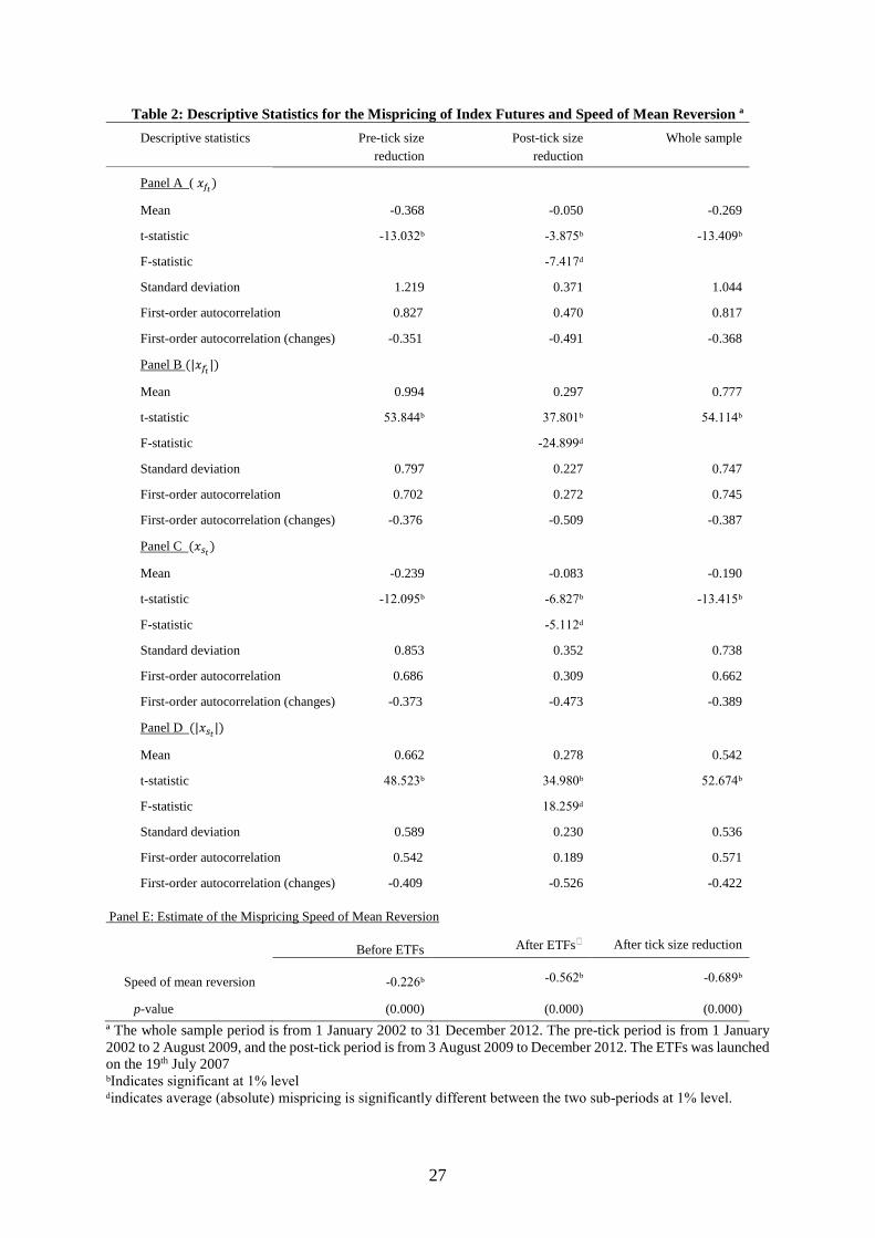
Table 2 reports the descriptive statistics of index futures mispricing for the whole period and for the sub-periods

before and after the implementation of lower tick sizes. Panels A and B show the descriptive statistics for

mispricing as implied by the stock index, while Panels C and D show the descriptive statistics for mispricing as

implied by the index futures.

Panel A shows that the mispricing of the FBM-FKLI is significantly lower (-0.050%) for the post tick period.

Similarly, in Panel B the average absolute mispricing (0.297%) is significantly lower for the post tick period

compared to the pre-tick period (0.994%). Further, it is interesting to note that the first-order autocorrelation of

the changes in mispricing and absolute mispricing are negative throughout the sample period. This provides

evidence of mean reversion in the series. The first-order autocorrelation of the mispricing series during the pre-

tick period is as high as 0.827, indicating high persistence in mispricing that declines significantly in the post-tick

period. The first-order autocorrelation of absolute mispricing indicates similar result. Panels C and D of Table 2

report the descriptive statistics of mispricing and absolute mispricing, calculated using equation (3). The findings

indicate that the mispricing and the absolute mispricing is significantly lower for the post-tick period. Similarly,

the first-order changes in autocorrelation are negative, indicating significant evidence of mean reversion,

discussion of which follows in the next paragraph.

16

<<Insert Table 2>>

Panel E of Table 2 reports the speed of mean reversion for mispricing as estimated in equation (3). It is interesting

to note that estimated speed of mean reversion is significantly higher after the introduction of ETFs. The mean

reverts to zero at a greater speed suggesting active arbitrage trading and efficient futures pricing in the post tick

period. Overall, the evidence suggests that the introduction of smaller tick sizes seems to have a positive effect

on the pricing efficiency of FBM-FKLI index futures.

4.1.3. Returns

Table 3 reports the descriptive statistics of spot index returns (���) and the FBM-FKLI index futures returns (���

)

for the whole as well as for the two sub-sample periods. The average returns in the spot market (0.034%) are

similar to the average futures returns (0.033%). However, the standard deviation (0.796%) of spot return is lower

than the standard deviation (1.018%) of futures returns, indicating the higher volatility of the futures market. For

the two sub periods too, the standard deviation of spot returns is relatively lower than in the futures. However, it

is worth noting that spot and futures returns volatility is higher in the pre-tick period compared to the post-tick

period.

It is evident that both returns series are negatively skewed. However, the skewness is lesser for the post-tick size

period. Also, the positive kurtosis decreases in the post-tick reduction period. This has significant implications. A

reduction in negative skewness with considerable reduction in positive kurtosis indicates a decline in the

probability of high negative returns in the post-tick period. Further, for the post-tick period; there is no significant

difference in the kurtosis between spot (4.849) and futures (4.669) which suggests that there is less likelihood of

abnormal positive or negative spot and futures returns for the period following tick size reduction.

<<Insert Table 3>>

4.2. Regression results

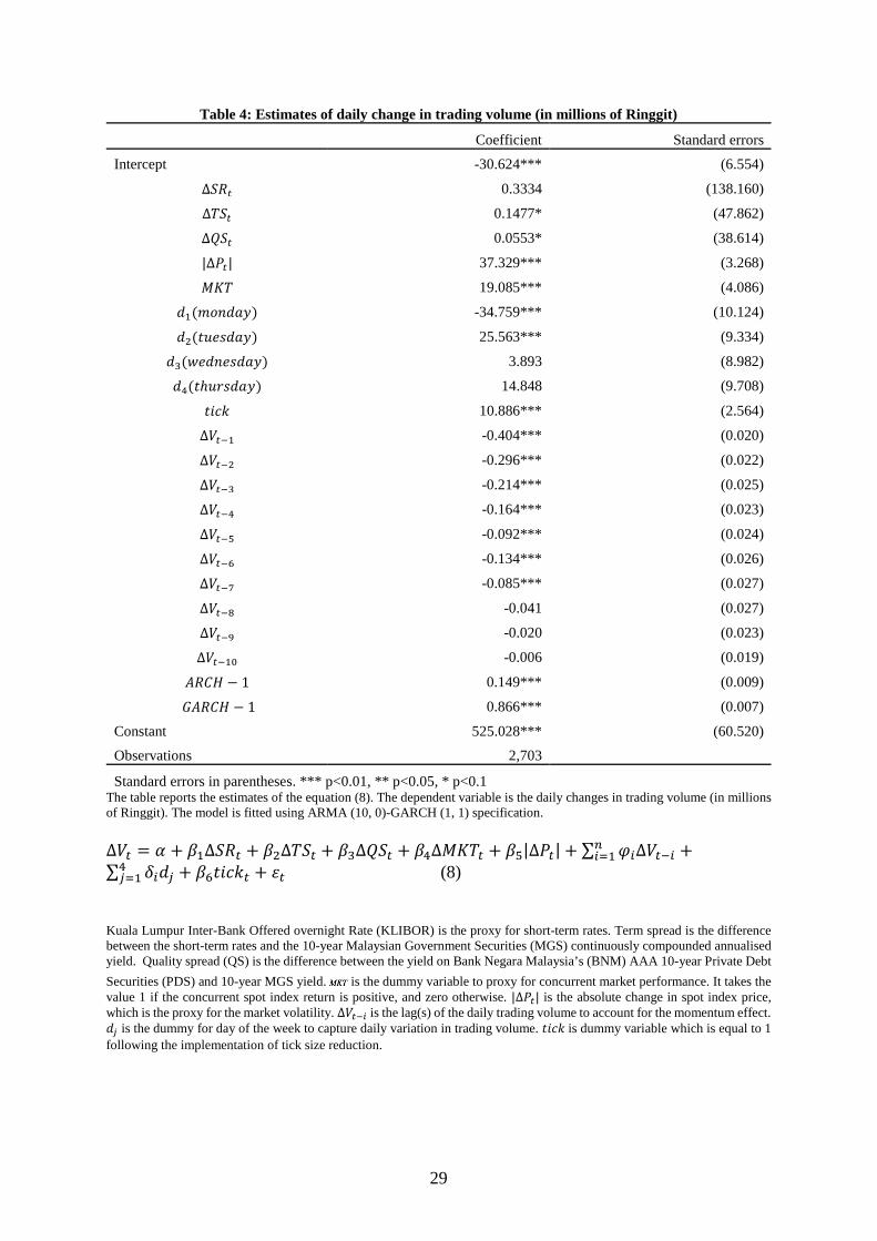
4.2.1. Impact of Tick Size on Trading Volume

Table 4 reports the ARIMA (10, 0, 0)-GARCH (1, 1) estimation of equation (8) for the scaled spot trading volume

(in millions of Ringgit). The intercept is significantly negative indicating a considerable decrease in trading

volume on Fridays of the week. The day of the week dummies are positive for Tuesday, Wednesday and Thursday,

while it is negative for Monday. This suggests that trading volume is lower during the beginning and towards the

end of the trading week whereas it is higher during the remaining days of the week. The term- spread and quality-

17

spread have positive coefficient signs and these are only marginally significant. However, both have little

influence on trading volume. Consistent with the previous studies, the volatility of spot returns is positively related

to the daily change in trading volume. Further, significant coefficients for the lags of trading volume changes

suggest the presence of momentum effects. Most importantly, the coefficient of the tick size dummy is positive

and statistically significant. This indicates that the reduction in tick sizes positively impacts upon the average

trading volume in the emerging Malaysian market.

<<Insert Table 4>>

4.2.2. Impact of Tick Size and Trading Volume on Mispricing

Table 5 reports the coefficient estimates of equation (9). There is evidence of mispricing as reflected by a

statistically significant constant term. Results show that the reduction of tick sizes reduces absolute daily

mispricing, as the coefficient for the tick dummy is negative and highly significant. The evidence also implies

that the reduction of tick sizes strengthens the spot-futures pricing relationship. Further, the introduction of the

ETFs seems to improve the pricing efficiency of index futures. As expected, the global financial crisis of 2008

has had an adverse impact on the index futures’ pricing efficiency.

The coefficient of futures volatility �����������

is positive and significant which suggests that new information is

incorporated with greater speed in the futures market. Significant positive autocorrelation coefficients (up to lag

6) indicate that mispricing is persistent. We note that the coefficients for unexpected volumes ������

and ���������

are positive and significant. This implies that the unexpected component of trading volumes represents trades

which widen futures mispricing. However, when inter-acted with the tick size change dummy, the coefficients are

negative and statistically significant. This suggests that tick size reduction leads to lower mispricing and the effect

is transmitted via an increase in the unexpected trading volume. The evidence suggests the reduction of tick sizes

improves the pricing efficiency of index futures.

<<Insert Table 5>>

Tables 6 & 7 report the results of quantile regressions for the absolute mispricing series as defined in equations

(2) and (3), respectively. The negatively significant OLS coefficients of the tick dummy indicate lower mispricing

after the tick size reduction. For the higher quantile regressions (� > 0.5), the coefficients of the tick size dummy

are again significantly negative, indicating improvements in pricing efficiency after tick size reduction. The results

also show that the introduction of ETFs reduce mispricing (� < 0.5). The quantile regression estimates show that

18

our results are robust and confirm that the reduction of tick sizes has improved the pricing efficiency of the FBM-

FKLI index futures in the Malaysian market.

<<<Insert Table 6 & 7 >>

4.2.3. Speed of adjustment

Finally, we provide evidence of the interactions between futures return and spot returns by investigating the lead-

lag relationship in terms of speed of adjustment while considering the possible effects of thin trading. We consider

five estimators of the speed of adjustment. The estimates are shown in Table 8 for the period before and after the

tick size reduction. The first four estimators are derived assuming that the intrinsic values follow a random walk

process. The estimators are: i) the co-variance ratio; ii) AR (1); iii) ARMA (1,1); iv) ARMA (1,X) and v) the fifth

speed of adjustment estimator assumes a non-random walk process.

The second column of Table 8 reports the cross-covariance estimates of the partial adjustment factor for the futures

and the spot markets. The futures seem to adjust to its equilibrium level at a higher speed, i.e. close to unity in

comparison to the spot. However, in the post tick period, the spot adjusts to its equilibrium level at a higher speed

compared to the period before the tick was reduced. This indicates that post the tick-size reduction, stock specific

information is reflected faster in the underlying market.

Columns three to five of Table 8 present the estimates of the speed of adjustment using three estimators based on

the ARMA specifications. In general, for the whole sample, the results show that the partial adjustment factor for

the index futures contract, �� , is significantly higher than for the spot, ��. Further, the results show that adjustment

factors that are significantly different from one are more frequently evident in the spot market. This implies that,

in general, the underlying market under-reacts to information. The AR (1) specification assumes an absence of

spread and noise effects. The findings show that for all the sub-sample periods the index futures incorporate

information ahead of the stock index. The estimates based on the ARMA(1,1) specification are calibrated

assuming an absence of thin trading effects. The findings indicate that when the noise and spread effects are

considered, both futures and spot over-react to information. It is noted that the spot adjusts at a considerably lower

rate following the tick size reduction. This implies that the tick size reduction has a dominant impact on the spot

market given that tick size reduction directly affects the spread.

The ARMA(1,X) specification takes into account the thin trading effect in the underlying. The estimates for the

futures are similar to the ARMA (1, 1) specification. The optimal lag order of moving average (X) is based on

Akaike Information Criterion (AIC). In line with the above findings, the result suggests that the reduction in tick

19

sizes facilitates traders in exploiting stock specific information, which strengthens the linkage between stock index

and index futures.

In the last two columns of Table 8, we report the model estimates that assume a non-random walk intrinsic value

process. The estimates are obtained by using non-linear least squares. Essentially, the intrinsic value process is a

random walk when the gamma value is equals to unity, i.e. the model will be the same as the ARMA (1, 1) model.

The results indicate that the speeds of adjustment are higher for the futures, similar to those reported previously.

In fact, for the futures, it is higher for the whole sample period and in each of the sub-periods. We show that the

speeds of adjustment for futures are significantly higher than one (over-reaction) and for the spot are significantly

less than one (under-reaction) throughout the whole and for sub-sample periods. This suggests that the speeds of

adjustments are sensitive to the specification of the underlying intrinsic value process. In general, the spot under-

reacts in relation to intrinsic values, while futures, in most instances, over-react, consistent with its price discovery

role.17 With regard to the coefficients in the intrinsic value process, ��, there is no evidence of over-or under-

reaction for both futures and spot. In general, futures’ speeds of adjustment are higher and closer to unity in

comparison to the spot’s speed of adjustment towards intrinsic values. Further, it can be established that the

intrinsic values for both markets follow a random walk process. The findings show that the partial adjustment

factor for the index futures contract, i.e., , and the partial adjustment factor for the stock index, i.e.,

are statistically significantly different from one at the 1% level. This suggests that both futures and spot markets

reflect less than full price adjustment.

<<Insert Table 8>>>

4.3 Robustness Check

We conduct a cointegration test using the Engle and Granger’s (1987) two-step single equation technique, which

rejects the null hypothesis of non-stationarity in the residuals. This indicates that there exists a cointegrating

relationship between stock and index futures, and thus there is a corresponding vector error correction model

(VECM).

Following Wahab & Lashgari (1993), we define the set of VECM as:

17 Indeed, Choy and Zhang (2010) find that in Hong Kong, the futures market plays a dominant role in price discovery.

20

∆�� = �� + ������� + ∑ ���(�)Δ�������� + ∑ ���(�)Δ����

���� + ���

(18)

∆�� = �� + ������� + ∑ ���(�)Δ�������� + ∑ ���(�)Δ����

���� + ���

(19)

where �� and �� are spot and futures prices, respectively, and the ∆ denotes the first-difference of the variable.

The lagged one-period equiblirium error, ����� measures the speed at which the left-hand variable reverts to its

equilibrium level. It also indicates the direction of the causal relationship. For example, if the coefficient for �����

in the first equation is zero, then �� does not respond to previous period’s adjustment towards long-run

equilibrium. The lagged first differences represent short-run effects of the previous period's returns on the current

period's returns. If �� is zero and all ���(�) are zero in the former equation, then ∆�� does not Granger cause ∆��.

Using Hannan and Quinn’s information criterion (HQIC) we select the autoregressive lag length as four. HQIC

statistics is used because it provides consistent estimates of p, the lag length, while AIC statistics tend to

overestimate the true lag length (Becketti, 2013). The numbers of lags are similar for both pre-and post-tick size

reduction. Diagnostic tests indicate no evidence of instability (examining Eigenvalues of the companion matrix

for bivariate VECM), nor there is evidence of autocorrelated errors (examining Lagrange-multiplier test for

autocorrelation).

The results of the fitted VECM for pre and post-tick size periods are displayed in the Tables A1 and A2 in the

appendix, respectively. For the pre-tick period, Panel B of Table A1 shows that for equation (18) the coefficients

of ���� are positive and significant. This implies that the spot index moves in the direction of the previous

movement of the futures price, underlining the price discovery role of the futures market for the spot market. For

the post-tick period, Panel B of Table A2, shows that the coefficients of ���� are insignificant. This indicates

that the lead of futures over spot weakens post-tick period. Prior to the tick reduction, error correction mechanism

occurs in both futures and spot markets as indicated by the significant coefficient on for both equations. In

comparison, it is significant only in the spot returns equation after the tick reduction. This indicates that following

the tick reduction the error correction mechanism is operating primarily through the adjustment of the spot prices

rather than the futures prices. Our findings are consistent with those reported for the Taiwan market by Lin, Chen

and Hwang (2002) who also find that most of the price discovery happens in index spot market.

5. Conclusions

The extant literature on the impact of lower tick sizes on spot market liquidity and futures pricing efficiency

provides a mixed picture. While many suggest that lower tick sizes reduce trading costs and improve efficiency,

some studies show that they adversely affect the liquidity as well pricing efficiency. Moreover, there is no

21

evidence hitherto on the impact of a major microstructure change introduced in the emerging Malaysian market.

As far as we are aware, this is the first study to provide evidence of the impact of the lowering of tick sizes on the

pricing efficiency of FBM-FKLI index futures.

Our findings show a significant increase in unexpected trading volume in the spot market and the speed of mean

reversion of the futures mispricing following the introduction of lower tick sizes. There are two components of

the unexpected spot trading volume. One represents arbitrage trades that serve to narrow down mispricing (Henker

and Martens, 2005). The other represents trades to exploit firm specific information, which may strengthen or

weaken the cash/futures pricing system, i.e. mispricing. If the unexpected spot trading volume is the result of

efficient incorporation of stock specific information, the mispricing is expected to narrow down (Alexander, 2008,

p.67; Chordia, Roll and Subrahmanyam, 2008). However, mispricing may widen if the unexpected spot trading

volume represents trades that cause the index futures to delay in responding to both firm specific and market-wide

information (Sutcliffe, 2006, p.162). Similarly, if arbitrageurs’ trades, in the composition of the unexpected spot

trading volume, exceed those trading on stock specific information, it is anticipated that mispricing will narrow

down and vice versa (Cummings and Frino, 2011). Thus, the speed at which the mispricing reverts to its mean i.e.

zero is determined by the composition of the unexpected spot trading volume. Therefore, the relationship between

the unexpected trading volume in the spot market and the speed of mean reversion of the futures mispricing is

attributed to that the fact that the futures mispricing process is, itself, a function of both the efficiency of pricing

in the futures and in the underlying spot markets. As the increased unexpected trading volume in the underlying

spot market would be anticipated to increase the informational efficiency of spot prices, the mean reversion in the

mispricing process would be anticipated to increase as the informational efficiency becomes more equivalent in

the two markets, assuming futures prices are the more efficient prices. We find that the speed at which the index

futures revert to equilibrium prices is significantly lower, while the stock index adjusts to its equilibrium level

much more quickly. This suggests that the reduction in tick size in the spot market leads to an increase in

equilibrium convergence relative to the futures market. The equilibrium convergence in the futures market

depends upon two factors; spot market efficiency/convergence and arbitrage processes. The combination of the

two factors in the futures market can cause this relative reversion difference. Overall, our findings show that the

reduction of tick sizes improves price discovery in the underlying spot market, while the leading role of index

futures is weaker in the post tick size period. This suggests that the futures market incorporates information more

rapidly than the spot market as the futures market leads the spot market both pre and post the tick size introduction.

However, the improvement in spot market price discovery post the tick size change indicates that the degree of

22

superior informational efficiency in the futures market relative to the spot is lesser with the result that the futures

market leads the spot market to a lesser extent post the tick size change. The empirical evidence reported in the

paper relating to the relationship between the unexpected trading volume in spot market and the speed of mean

reversion of the futures mispricing offers useful policy implications for other emerging markets regarding the

lowering of tick sizes and its effects on liquidity and pricing efficiency.

23

References Alexander C (2008) Market risk analysis: pricing, hedging and trading financial instruments. John Wiley & Sons,

London

Amihud Y, Mendelson H (1987) Trading Mechanisms and Stock Returns: An Empirical Investigation. The

Journal of Finance 42(3): 533–553

Bacidore JM (1997) The Impact of Decimalization on Market Quality: An Empirical Investigation of the Toronto

Stock Exchange. Journal of Financial Intermediation 6(2): 92–120

Beaulieu M, Ebrahim SK, Morgan IG (2003) Does Tick Size Influence Price Discovery? Evidence from Toronto

Stock Exchange. The Journal of Futures Market 23(1): 49-66

Becketti S, (2013) Introduction to time series using Stata. Stata Press, Texas

Bekaert G, Harvey CR, Lundblad C (2007) Liquidity and Expected Returns: Lessons from Emerging Markets,

Review of Financial Studies 20(6): 1783–1831

Bessembinder H, Seguin PJ (1992) Futures Trading Activity and Stock Price Volatility. The Journal of Finance

47(5): 2015–2034

Boellen NPB, Whaley RE (1998) Are “teenies” better? The Journal of Portfolio Management 25(1): 10–24

Bourghelle D, Declerck F (2004) Why markets should not necessarily reduce the tick size. Journal of Banking &

Finance 28(2): 373-398

Brennan MJ, Schwartz (1990) Arbitrage in stock index futures. Journal of Business 63: 7–31

Brenner M, Subrahmanyam MG, Uno J (1989) Stock index futures arbitrage in the Japanese markets. Japan and

the world economy 1(3): 303–330

Brooks C, Persand G (2001) Seasonality in Southeast Asian stock markets: some new evidence on day-of-the-

week effects. Applied Economics Letters 8(3): 155–158

Butterworth D, Holmes P (2000) Mispricing in stock index futures contracts: evidence for the FTSE 100 and

FTSE mid 250 contracts. Applied Economics Letters 7(12): 795–801

Chen WP, Chou RK, Chung H (2009) Decimalization, ETFs and futures pricing efficiency. Journal of Futures

Markets 29(2): 157–178

Chen YL, Gau YF (2009) Tick sizes and relative rates of price discovery in stock, futures, and options markets:

Evidence from the Taiwan Stock Exchange. Journal of Futures Markets 29(1): 74-93

Chordia T, Roll R, Subrahmanyam A (2008) Liquidity and market efficiency. Journal of Financial Economics

87(2): 249–268

Chordia T, Roll R, Subrahmanyam A (2001) Market Liquidity and Trading Activity. The Journal of Finance

56(2): 501–530

Choy SK, Zhang H (2010) Trading costs and price discovery, Review of Quantitative Finance & Accounting

34(1): 37

Chu QC, Hsieh WLG (2002) Pricing efficiency of the S&P 500 index market: Evidence from the Standard &

Poor's Depositary Receipts. Journal of Futures Markets 22(9): 877–900

Chung DY, Hrazdil K (2010) Liquidity and market efficiency: Analysis of NASDAQ firms. Global Finance

Journal 21(3): 262–274

Chung KH, Kim KA, Kitsabunnarat P (2005) Liquidity and quote clustering in a market with multiple tick sizes.

Journal of Financial Research 28(2): 177–195

Cummings JR, Frino A (2011) Index arbitrage and the pricing relationship between Australian stock index futures

24

and their underlying shares. Accounting & Finance 51(3): 661–683

Foster FD, Viswanathan S (1990) A theory of the interday variations in volume, variance, and trading costs in

securities markets. Review of Financial Studies 3(4): 593–624

Gwilym OA, Mcmanus I, Thomas S (2005) Fractional versus decimal pricing: Evidence from the UK Long Gilt

futures market. Journal of Futures Market 25: 419–442.

Harris LE, (1997) Decimalization: A review of the arguments and evidence. Unpublished working paper,

University of Southern California

Harris LE, (1994) Minimum price variations, discrete bid-ask spreads, and quotation sizes. Review of Financial

Studies 7(1): 149–178

Henker T, Martens M, (2005) Index futures arbitrage before and after the introduction of sixteenths on the NYSE.

Journal of Empirical Finance 12(3): 353–373

Hsieh TY,Chuang SS, Lin CC (2008) Impact of Tick-Size Reduction on the Market Liquidity — Evidence from

the Emerging Order-Driven Market, Review of Pacific Basin Financial Markets and Policies 11: 591–616

Jones CM, Lipson ML (2001) Sixteenths: direct evidence on institutional execution costs. Journal of Financial

Economics 59(2): 253–278

Karpoff JM (1987) The Relation between Price Changes and Trading Volume: A Survey. Journal of Financial

and Quantitative Analysis 22(1): 109–126

Kurov A, Lasser DJ (2002) The effect of the introduction of Cubes on the Nasdaq 100 index spot futures pricing

relationship. Journal of Futures Markets 22(3): 197–218

Kurov A, Zabotina T (2005) Is it time to reduce the minimum tick sizes of the E-mini futures? Journal of Futures

Markets 25(1): 79-104

Kurov A (2008) Tick size reduction, execution costs, and informational efficiency in the regular and E-mini

Nasdaq 100 index futures markets. Journal of Futures Markets 28(9): 871-888

Lau ST, McInish TH (1995) Reducing tick sizes on the Singapore Stock Exchange. Pacific-Basin Finance Journal

3(4): 485–496

Lepone A, Wong JB (2017) Pseudo market-makers, market quality and the minimum tick size. International

Review of Economics & Finance 47: 88-100

Lin CC, Cheng CY, Hwang DY (2002) Does Index Futures Dominate Index Spot? Evidence from Taiwan Market.

Review of Pacific Basin Financial Markets and Policies 05(02): 255-275

MacKinlay AC, Ramaswamy K (1988) Index-futures arbitrage and the behavior of stock index futures prices.

Review of Financial Studies 1(2): 137–158

MacKinnon G, Nemiroff H (2004) Tick size and the returns to providing liquidity. International Review of

Economics & Finance 13(1): 57–73

Park TH, Switzer LN (1995) Index participation units and the performance of index futures markets: Evidence

from the Toronto 35 index participation units market. Journal of Futures Markets 15(2): 187–200.

Pavabutr P, Prangwattananon S (2009) Tick size change on the stock exchange of Thailand. Review of

Quantitative Finance and Accounting 32(4): 351–371

Pok WC, Poshakwale SS, Ford JL (2009) Stock index futures hedging in the emerging Malaysian market. Global

Finance Journal 20(3): 273–288

Puttonen V (1993) Stock index futures arbitrage in Finland: Theory and evidence in a new market. European

25

Journal of Operational Research 68(3): 304–317

Roll R, Schwartz E, Subrahmanyam A (2007) Liquidity and the Law of One Price: The Case of the Futures Cash

Basis. The Journal of Finance 62(5): 2201–2234

Ronen T, Weaver DG (2001) Teenies anyone? Journal of Financial Markets 4(3): 231–260

Sutcliffe CMS (2006) Stock Index Futures , Ashgate Publishing Company, London

Switzer LN, Varson PL, Samia Z (2000) Standard and Poor’s depository receipts and the performance of the S&P

500 index futures market. Journal of Futures Markets 20(8): 705–716

Theobald M, Yallup P (1998) Measuring cash-futures temporal effects in the UK using partial adjustment factors.

Journal of Banking & Finance 22(2): 221–243

Theobald M, Yallup P (2004) Determining security speed of adjustment coefficients. Journal of Financial Markets

7(1): 75-96

Verousis T, Perotti P, Sermpinis G (2018) One size fits all? High frequency trading, tick size changes and the

implications for exchanges: market quality and market structure considerations, Review of Quantitative

Finance & Accounting 50: 353–392

Wahab M, Lashgari M (1993) Price dynamics and error correction in stock index and stock index futures markets:

A cointegration approach, Journal of Futures Markets 13(7): 711–742

Yadav PK, Pope PF (1994) Stock index futures mispricing: profit opportunities or risk premia? Journal of Banking

& Finance 18(5): 921–953

26

Table 1: Descriptive Statistics of Trading Activity and Absolute Percentage Daily Changes in Trading

Activity ª

Pre-tick size reduction Post-tick size reduction Whole Sample

Panel A: FBM-KLCI Stock Index

A1: Level of Spot Volume (in Thousands of Ringgit Malaysia)

N 1864 840 2704

Mean 566,505.790 777,680.544 632,107.415

Std. Dev. (�) 413,242.444 279,378.690 389,205.056

Coefficient of variation (��)ᵇ 0.729 0.359 0.616

Minimum 19,029.000 254,268.000 19,029.00

Maximum 3,300,398.000 2,744,341.00 3,300,398.00

A2: Absolute daily % changes in Spot Volume

N 1863 840 2703

Mean 25.665 23.302 24.931

Std. Dev. (�) 28.057 24.898 27.132

Minimum 0.017 0.001 0.001

Maximum 483.825 312.214 483.825

Panel B: FBM-FKLI Index Futures

B1: Level of Futures Volume (in Thousands of Ringgit Malaysia)

N 1864 840 2704

Mean 247,830.20 464,524.50 315,146.50

Std. Dev. (�) 258,791.40 257,081.00 277,008.30

Coefficient of variation (��)ᵇ 1.044 0.553 0.879

Minimum 0.000 0.000 0.000

Maximum 1,705,703.00 1,985,066.00 1,985,066.00

B2: Absolute daily % changes in Futures Volume

N 1863 840 2703

Mean 13.54413 10.8734 12.7159

Std. Dev. (�) 70.94209 56.729 66.85941

Minimum 0.001 0.011 0.001

Maximum 1,438.325 422.534 1,438.325Note: ª The whole sample period is from 2 January 2002 to 31 December 2012. The pre-tick period is from 2 January 2002 to 2 August 2009, and the post-tick period is from 3 August 2009 to 31 December 2012.

ᵇThe coefficient of variance is calculated as: �� =�

�

Table 1 provides summary statistics of daily trading activities for the constituents stocks and the index futures, before and after the reduction of tick sizes as well as for the whole sample period considered in the study. Panel A shows the summary statistics for the value of shares traded in Malaysian Ringgit (RM), while, Panel B shows the summary statistics for the value of futures contracts traded during the day. The volume of trading of both constituent stocks and futures contracts is significantly higher in post-tick period. The �� for both are lower in the post tick size period. .

27

Table 2: Descriptive Statistics for the Mispricing of Index Futures and Speed of Mean Reversion ª

Descriptive statistics Pre-tick size

reduction

Post-tick size

reduction

Whole sample

Panel A ( ���)

Mean -0.368 -0.050 -0.269

t-statistic -13.032ᵇ -3.875ᵇ -13.409ᵇ

F-statistic -7.417ᵈ

Standard deviation 1.219 0.371 1.044

First-order autocorrelation 0.827 0.470 0.817

First-order autocorrelation (changes) -0.351 -0.491 -0.368

Panel B (|���|)

Mean 0.994 0.297 0.777

t-statistic 53.844ᵇ 37.801ᵇ 54.114ᵇ

F-statistic -24.899ᵈ

Standard deviation 0.797 0.227 0.747

First-order autocorrelation 0.702 0.272 0.745

First-order autocorrelation (changes) -0.376 -0.509 -0.387

Panel C (���)

Mean -0.239 -0.083 -0.190

t-statistic -12.095ᵇ -6.827ᵇ -13.415ᵇ

F-statistic -5.112ᵈ

Standard deviation 0.853 0.352 0.738

First-order autocorrelation 0.686 0.309 0.662

First-order autocorrelation (changes) -0.373 -0.473 -0.389

Panel D (|���|)

Mean 0.662 0.278 0.542

t-statistic 48.523ᵇ 34.980ᵇ 52.674ᵇ

F-statistic 18.259ᵈ

Standard deviation 0.589 0.230 0.536

First-order autocorrelation 0.542 0.189 0.571

First-order autocorrelation (changes) -0.409 -0.526 -0.422

Panel E: Estimate of the Mispricing Speed of Mean Reversion

Before ETFs After ETFs▴ After tick size reduction

Speed of mean reversion -0.226ᵇ -0.562ᵇ -0.689ᵇ

p-value (0.000) (0.000) (0.000)

ª The whole sample period is from 1 January 2002 to 31 December 2012. The pre-tick period is from 1 January 2002 to 2 August 2009, and the post-tick period is from 3 August 2009 to December 2012. The ETFs was launched on the 19th July 2007 ᵇIndicates significant at 1% level ᵈindicates average (absolute) mispricing is significantly different between the two sub-periods at 1% level.

28

Note: Table 2 reports the descriptive statistics and the mean reversion properties of the mispricing of index futures. Panel A and Panel B report the (absolute) mispricing as implied by the underlying index (Eq. (2)), while Panel C and Panel D report the (absolute) mispricing as implied by the index futures (Eq. (3)). In addition, Panel E reports the estimate of the mispricing speed of mean reversion as characterised in equation (4). Panels C and D of Table 2 report the descriptive statistics of mispricing and absolute mispricing calculated using equation (3). Panel E of Table 2 reports the speed of mean reversion for mispricing as estimated in equation (3).

Table 3: Descriptive statistics of the spot index and the index futures returnsª

Descriptive

Statistic ���

���

Pre-tick size

reduction

Post-tick size

reduction

Whole sample Pre-tick size

reduction

Post-tick size

reduction

Whole sample

1863 840 2703 1863 840 2703

Mean 0.029 0.043 0.034 0.028 0.043 0.033

Std. dev. 0.879 0.572 0.796 1.137 0.683 1.018

Skewness -0.952 -0.449 -0.942 -0.528 -0.370 -0.550

Kurtosis 14.249 4.849 14.991 6.468 4.669 7.246

Jarque-Bera 10103.597 147.841 16592.987 1020.174 116.578 2166.851

ᵇp-values 0.000 0.000 0.000 0.000 0.000 0.000

ª The whole sample period runs from 2 January 2002 to 31 December 2012. While, the pre-and post-tick size reduction periods run from 2 January 2002 to 2 August 2009, and from 3 August 2009 to 31 December 2012,

respectively. The returns of the stock index and index futures are defined as ���= 100 ∗ ln (

��

����) and ���

= 100 ∗

ln (��

����), respectively.

ᵇ p-values for the Jarque-Bera statistics

29

Table 4: Estimates of daily change in trading volume (in millions of Ringgit)

Coefficient Standard errors

Intercept -30.624*** (6.554)

∆��� 0.3334 (138.160)

∆��� 0.1477* (47.862)

∆��� 0.0553* (38.614)

|∆��| 37.329*** (3.268)

��� 19.085*** (4.086)

��(������) -34.759*** (10.124)

��(�������) 25.563*** (9.334)

��(���������) 3.893 (8.982)

��(�ℎ������) 14.848 (9.708)

���� 10.886*** (2.564)

∆���� -0.404*** (0.020)

∆���� -0.296*** (0.022)

∆���� -0.214*** (0.025)

∆���� -0.164*** (0.023)

∆���� -0.092*** (0.024)

∆���� -0.134*** (0.026)

∆���� -0.085*** (0.027)

∆���� -0.041 (0.027)

∆���� -0.020 (0.023)

∆����� -0.006 (0.019)

���� − 1 0.149*** (0.009)

����� − 1 0.866*** (0.007)

Constant 525.028*** (60.520)

Observations 2,703

Standard errors in parentheses. *** p<0.01, ** p<0.05, * p<0.1 The table reports the estimates of the equation (8). The dependent variable is the daily changes in trading volume (in millions of Ringgit). The model is fitted using ARMA (10, 0)-GARCH (1, 1) specification.

Δ�� = � + ��∆��� + ��∆��� + ��∆��� + ��∆���� + ��|∆��| + ∑ ��Δ���� +����

∑ ���� + ������� + ������ (8)

Kuala Lumpur Inter-Bank Offered overnight Rate (KLIBOR) is the proxy for short-term rates. Term spread is the difference between the short-term rates and the 10-year Malaysian Government Securities (MGS) continuously compounded annualised yield. Quality spread (QS) is the difference between the yield on Bank Negara Malaysia’s (BNM) AAA 10-year Private Debt

Securities (PDS) and 10-year MGS yield. is the dummy variable to proxy for concurrent market performance. It takes the value 1 if the concurrent spot index return is positive, and zero otherwise. |∆��| is the absolute change in spot index price, which is the proxy for the market volatility. ∆���� is the lag(s) of the daily trading volume to account for the momentum effect. �� is the dummy for day of the week to capture daily variation in trading volume. ���� is dummy variable which is equal to 1

following the implementation of tick size reduction.

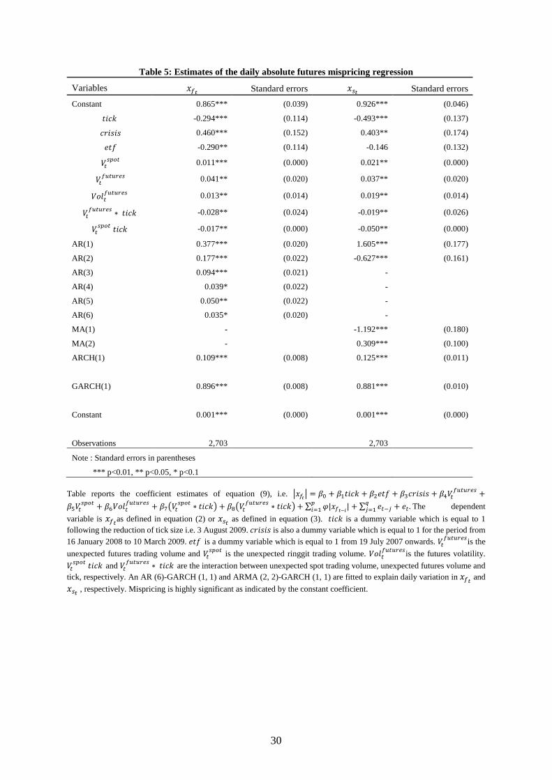
30

Table 5: Estimates of the daily absolute futures mispricing regression

Variables ��� Standard errors ��� Standard errors

Constant 0.865*** (0.039) 0.926*** (0.046)

���� -0.294*** (0.114) -0.493*** (0.137)

������ 0.460*** (0.152) 0.403** (0.174)

��� -0.290** (0.114) -0.146 (0.132)

������ 0.011*** (0.000) 0.021** (0.000)

��������� 0.041** (0.020) 0.037** (0.020)

����������� 0.013** (0.014) 0.019** (0.014)

���������

∗ ���� -0.028** (0.024) -0.019** (0.026)

������

���� -0.017** (0.000) -0.050** (0.000)

AR(1) 0.377*** (0.020) 1.605*** (0.177)

AR(2) 0.177*** (0.022) -0.627*** (0.161)

AR(3) 0.094*** (0.021) -

AR(4) 0.039* (0.022) -

AR(5) 0.050** (0.022) -

AR(6) 0.035* (0.020) -

MA(1) - -1.192*** (0.180)

MA(2) - 0.309*** (0.100)

ARCH(1) 0.109*** (0.008) 0.125*** (0.011)

GARCH(1) 0.896*** (0.008) 0.881*** (0.010)

Constant 0.001*** (0.000) 0.001*** (0.000)

Observations 2,703 2,703

Note : Standard errors in parentheses

*** p<0.01, ** p<0.05, * p<0.1

Table reports the coefficient estimates of equation (9), i.e. ����� = �� + ������ + ����� + �������� + ����

�������+

��������

+ �������������

+ ���������

∗ ����� + ������������

∗ ����� + ∑ �|�����|

���� + ∑ ���� + ��

���� . The dependent

variable is ���as defined in equation (2) or ���

as defined in equation (3). ���� is a dummy variable which is equal to 1

following the reduction of tick size i.e. 3 August 2009. ������ is also a dummy variable which is equal to 1 for the period from

16 January 2008 to 10 March 2009. ��� is a dummy variable which is equal to 1 from 19 July 2007 onwards. ���������

is the

unexpected futures trading volume and ������

is the unexpected ringgit trading volume. �����������

is the futures volatility.

������

���� and ���������

∗ ���� are the interaction between unexpected spot trading volume, unexpected futures volume and

tick, respectively. An AR (6)-GARCH (1, 1) and ARMA (2, 2)-GARCH (1, 1) are fitted to explain daily variation in ��� and

��� , respectively. Mispricing is highly significant as indicated by the constant coefficient.

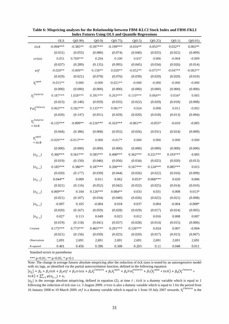
31

Table 6: Mispricing analyses for the Relationship between FBM-KLCI Stock Index and FBM-FKLI Index Futures Using OLS and Quantile Regressions

OLS Q(0.99) Q(0.9) Q(0.75) Q(0.5) Q(0.25) Q(0.1) Q(0.01)

���� -0.094*** -0.385** -0.397*** -0.199*** -0.016** 0.053** 0.032** 0.002**

(0.031) (0.055) (0.080) (0.074) (0.040) (0.025) (0.022) (0.009)

������ 0.051 0.769*** 0.204 0.100 0.037 0.006 -0.004 -0.009

(0.037) (0.289) (0.135) (0.095) (0.045) (0.034) (0.026) (0.014)

��� -0.020** -0.009** 0.158** 0.028** -0.052** -0.075** -0.047** -0.002**

(0.029) (0.021) (0.078) (0.076) (0.039) (0.029) (0.020) (0.010)

������ -0.015** 0.000 -0.000 -0.021** -0.000 -0.000 -0.000 -0.000

(0.000) (0.000) (0.000) (0.000) (0.000) (0.000) (0.000) (0.000)

��������� 0.187*** 1.028*** 0.391*** 0.263*** 0.110*** 0.064** 0.034* 0.005

(0.023) (0.140) (0.059) (0.035) (0.022) (0.029) (0.018) (0.008)

����������� 0.063*** 0.582*** 0.135*** 0.061** 0.024 0.008 0.011 -0.002

(0.020) (0.147) (0.051) (0.029) (0.020) (0.018) (0.013) (0.004)

���������

∗ ����-0.135*** -0.899** -0.216*** -0.163*** -0.061** -0.055* -0.010 -0.005

(0.044) (0.386) (0.068) (0.055) (0.026) (0.031) (0.024) (0.009)

������

∗ ����-0.026*** -0.013*** 0.000 -0.017* 0.000 0.000 0.000 0.000

(0.000) (0.000) (0.000) (0.000) (0.000) (0.000) (0.000) (0.000)

|�����| 0.360*** 0.561*** 0.585*** 0.498*** 0.362*** 0.221*** 0.103*** 0.005

(0.019) (0.150) (0.046) (0.056) (0.034) (0.025) (0.020) (0.013)

|�����| 0.185*** 0.386** 0.187*** 0.200*** 0.167*** 0.124*** 0.085*** 0.015

(0.020) (0.177) (0.039) (0.044) (0.026) (0.022) (0.016) (0.009)

|�����| 0.044** 0.009 0.011 0.062 0.053* 0.068*** 0.020 0.006

(0.021) (0.116) (0.052) (0.042) (0.032) (0.025) (0.014) (0.010)

|�����| 0.069*** 0.104 0.126*** 0.084** 0.033 0.031 0.008 0.013*

(0.021) (0.107) (0.034) (0.040) (0.026) (0.022) (0.021) (0.008)

|�����| -0.007 0.105 -0.004 0.018 0.037 0.004 -0.004 -0.008*

(0.020) (0.167) (0.059) (0.028) (0.029) (0.017) (0.024) (0.005)

|�����| 0.027 0.113 0.049 0.023 0.012 0.016 0.008 0.007

(0.019) (0.118) (0.041) (0.037) (0.028) (0.014) (0.015) (0.006)

Constant 0.175*** 0.773*** 0.465*** 0.291*** 0.126*** 0.024 0.007 -0.004

(0.021) (0.156) (0.039) (0.025) (0.020) (0.017) (0.015) (0.007)

Observations 2,691 2,691 2,691 2,691 2,691 2,691 2,691 2,691

R-squared 0.401 0.456 0.396 0.308 0.203 0.11 0.048 0.011

Standard errors in parentheses

*** p<0.01, ** p<0.05, * p<0.1 Note: The change in average futures absolute mispricing after the reduction of tick sizes is tested by an autoregressive model with six lags, as identified via the partial autocorrelation function, defined in the following equation:

����� = �� + ������ + ����� + �������� + ����

�������+ ����

����+ ������

�������+ �����

����∗ ����� + �����

�������∗

����� + ∑ �|�����|

���� + ��

|���| is the average absolute mispricing, defined in equation (2), at time � ; ���� is a dummy variable which is equal to 1

following the reduction of tick size i.e. 3 August 2009. ������ is also a dummy variable which is equal to 1 for the period from

16 January 2008 to 10 March 2009. ��� is a dummy variable which is equal to 1 from 19 July 2007 onwards. ���������

is the

32

unexpected futures trading volume and ������

is the unexpected ringgit trading volume. �����������

is the futures volatility.

������

∗ ���� and ���������

∗ ���� are the interaction between unexpected spot trading volume, unexpected futures volume and tick dummy, respectively. In addition, six lags of the dependent variable in the regression model are employed to eliminate autocorrelation in the residuals. OLS method and linear quantile regression are adopted to estimate this equation.

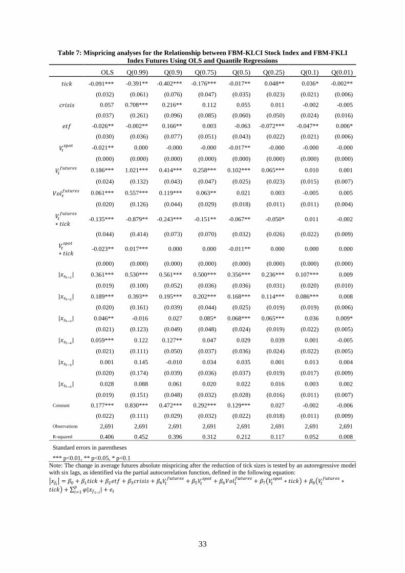
33

Table 7: Mispricing analyses for the Relationship between FBM-KLCI Stock Index and FBM-FKLI Index Futures Using OLS and Quantile Regressions

OLS Q(0.99) Q(0.9) Q(0.75) Q(0.5) Q(0.25) Q(0.1) Q(0.01)

���� -0.091*** -0.391** -0.402*** -0.176*** -0.017** 0.048** 0.036* -0.002**

(0.032) (0.061) (0.076) (0.047) (0.035) (0.023) (0.021) (0.006)

������ 0.057 0.708*** 0.216** 0.112 0.055 0.011 -0.002 -0.005

(0.037) (0.261) (0.096) (0.085) (0.060) (0.050) (0.024) (0.016)

��� -0.026** -0.002** 0.166** 0.003 -0.063 -0.072*** -0.047** 0.006*

(0.030) (0.036) (0.077) (0.051) (0.043) (0.022) (0.021) (0.006)

������ -0.021** 0.000 -0.000 -0.000 -0.017** -0.000 -0.000 -0.000

(0.000) (0.000) (0.000) (0.000) (0.000) (0.000) (0.000) (0.000)

��������� 0.186*** 1.021*** 0.414*** 0.258*** 0.102*** 0.065*** 0.010 0.001

(0.024) (0.132) (0.043) (0.047) (0.025) (0.023) (0.015) (0.007)

����������� 0.061*** 0.557*** 0.119*** 0.063** 0.021 0.003 -0.005 0.005

(0.020) (0.126) (0.044) (0.029) (0.018) (0.011) (0.011) (0.004)

���������

∗ ����-0.135*** -0.879** -0.243*** -0.151** -0.067** -0.050* 0.011 -0.002

(0.044) (0.414) (0.073) (0.070) (0.032) (0.026) (0.022) (0.009)

������

∗ ����-0.023** 0.017*** 0.000 0.000 -0.011** 0.000 0.000 0.000

(0.000) (0.000) (0.000) (0.000) (0.000) (0.000) (0.000) (0.000)

|�����| 0.361*** 0.530*** 0.561*** 0.500*** 0.356*** 0.236*** 0.107*** 0.009

(0.019) (0.100) (0.052) (0.036) (0.036) (0.031) (0.020) (0.010)

|�����| 0.189*** 0.393** 0.195*** 0.202*** 0.168*** 0.114*** 0.086*** 0.008

(0.020) (0.161) (0.039) (0.044) (0.025) (0.019) (0.019) (0.006)

|�����| 0.046** -0.016 0.027 0.085* 0.068*** 0.065*** 0.036 0.009*

(0.021) (0.123) (0.049) (0.048) (0.024) (0.019) (0.022) (0.005)

|�����| 0.059*** 0.122 0.127** 0.047 0.029 0.039 0.001 -0.005

(0.021) (0.111) (0.050) (0.037) (0.036) (0.024) (0.022) (0.005)

|�����| 0.001 0.145 -0.010 0.034 0.035 0.001 0.013 0.004

(0.020) (0.174) (0.039) (0.036) (0.037) (0.019) (0.017) (0.009)

|�����| 0.028 0.088 0.061 0.020 0.022 0.016 0.003 0.002

(0.019) (0.151) (0.048) (0.032) (0.028) (0.016) (0.011) (0.007)

Constant 0.177*** 0.830*** 0.472*** 0.292*** 0.129*** 0.027 -0.002 -0.006

(0.022) (0.111) (0.029) (0.032) (0.022) (0.018) (0.011) (0.009)

Observations 2,691 2,691 2,691 2,691 2,691 2,691 2,691 2,691

R-squared 0.406 0.452 0.396 0.312 0.212 0.117 0.052 0.008

Standard errors in parentheses

*** p<0.01, ** p<0.05, * p<0.1 Note: The change in average futures absolute mispricing after the reduction of tick sizes is tested by an autoregressive model with six lags, as identified via the partial autocorrelation function, defined in the following equation:

����� = �� + ������ + ����� + �������� + ����

�������+ ����

����+ ������

�������+ �����

����∗ ����� + �����

�������∗

����� + ∑ �|�����|

���� + ��

34

Table 8: Estimates of partial-adjustment factorsa

Sample frame �� Non-Random Walk

Cross-covariance ratio AR(1) ARMA(1,1) ARMA(1,X)ᵇ �� ��

Whole data set

�� 0.988 1.050* 1.305 1.305 1.000** 1.176**

�� 0.744 0.869* 0.830 0.869* 1.000** 0.721**

Pre-tick

�� 0.993 1.048* 1.192 1.192 1.000** 1.182**

�� 0.743 0.867* 1.134 0.737 1.000** 0.714**

Post-tick

�� 0.959 1.068* 1.716* 1.716* 1.000** 1.145**

�� 0.751 0.876* 0.692 0.876* 1.000** 0.763**

The whole sample frame comprises the period from 2 January 2002 to 31 December 2012; pre-tick period is from 2 Jan 2002 - 2 August 2009 and post-tick is from 3 Aug 2009 to 31 Dec 2012. ᵇ The optimal MA components are determined by the Akaike Information Criterion (AIC). * Statistically significantly different from one at the 5% significance level. Equivalently, (1 − ��) is significantly different from zero at 5% level. **Statistically significantly different from zero at the 5% significance level.

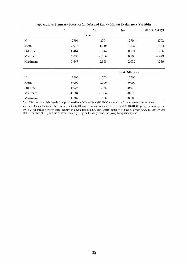
35

Appendix A: Summary Statistics for Debt and Equity Market Explanatory Variables

�� �� �� Stocks (%/day)

Levels

N 2704 2704 2704 2703

Mean 2.977 1.210 1.137 0.034

Std. Dev. 0.464 0.744 0.171 0.796

Minimum 2.030 -0.506 0.598 -9.979

Maximum 3.647 2.695 2.032 4.259

First Differences

N 2703 2703 2703

Mean 0.000 -0.000 -0.000

Std. Dev. 0.023 0.065 0.079

Minimum -0.784 -0.604 -0.676

Maximum 0.307 0.738 0.588 �� : Yield on overnight Kuala Lumpur Inter-Bank Offered Rate (KLIBOR), the proxy for short-term interest rates.

�� : Yield spread between the constant maturity 10-year Treasury bond and the overnight KLIBOR, the proxy for term spread.

�� : Yield spread between Bank Negara Malaysia (BNM), i.e. The Central Bank of Malaysia, Grade AAA 10-year Private Debt Securities (PDS) and the constant maturity 10-year Treasury bond, the proxy for quality spread.

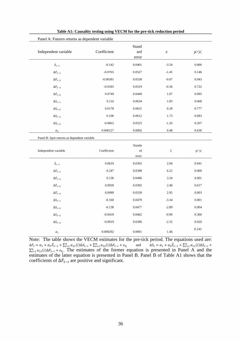
36

Table A1: Causality testing using VECM for the pre-tick reduction period

Panel A: Futures returns as dependent variable

Independent variable Coefficient

Stand

ard

error

� p>¦z¦

�̂��� -0.142 0.0401 -3.54 0.000

∆���� -0.0765 0.0527 -1.45 0.146

∆���� -0.00381 0.0538 -0.07 0.943

∆���� -0.0185 0.0519 -0.36 0.722

∆���� 0.0749 0.0449 1.67 0.095

∆���� 0.116 0.0634 1.83 0.068

∆���� 0.0178 0.0631 0.28 0.777

∆���� 0.106 0.0612 1.73 0.083

∆���� -0.0662 0.0525 -1.26 0.207

�� 0.000127 0.0002 0.48 0.630

Panel B: Spot returns as dependent variable

Independent variable Coefficient

Standa

rd

error

p>¦z¦

�̂��� 0.0619 0.0303 2.04 0.041

∆���� 0.247 0.0398 6.22 0.000

∆���� 0.136 0.0406 3.34 0.001

∆���� 0.0939 0.0392 2.40 0.017

∆���� 0.0999 0.0339 2.95 0.003

∆���� -0.160 0.0479 -3.34 0.001

∆���� -0.138 0.0477 -2.89 0.004

∆���� -0.0418 0.0462 -0.90 0.366

∆���� -0.0919 0.0396 -2.32 0.020

�� 0.000292 0.0001 1.46 0.143

Note: The table shows the VECM estimates for the pre-tick period. The equations used are: ∆�� = �� + ������� + ∑ ���(�)Δ����

���� + ∑ ���(�)Δ����

���� + ���

and ∆�� = �� + ������� + ∑ ���(�)Δ�������� +

∑ ���(�)Δ�������� + ���

. The estimates of the former equation is presented in Panel A and the estimates of the latter equation is presented in Panel B. Panel B of Table A1 shows that the coefficients of ���� are positive and significant.

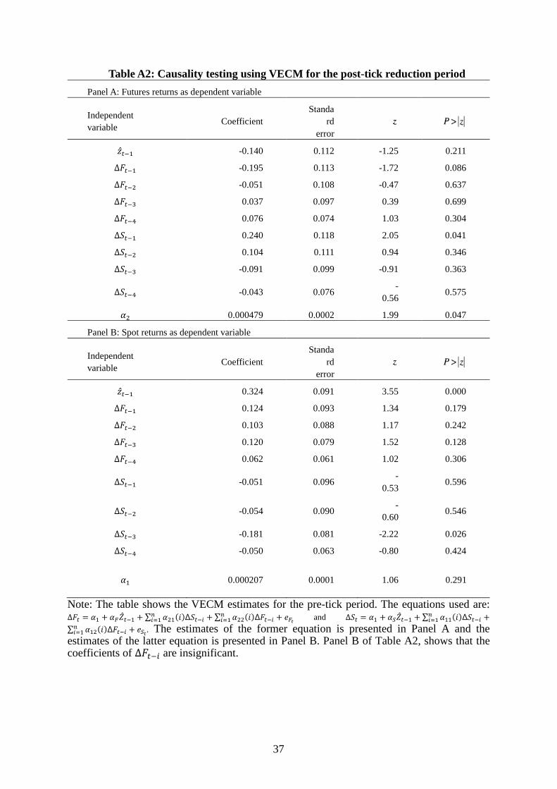
37

Table A2: Causality testing using VECM for the post-tick reduction period

Panel A: Futures returns as dependent variable

Independent

variableCoefficient

Standa

rd

error

�̂��� -0.140 0.112 -1.25 0.211

∆���� -0.195 0.113 -1.72 0.086

∆���� -0.051 0.108 -0.47 0.637

∆���� 0.037 0.097 0.39 0.699

∆���� 0.076 0.074 1.03 0.304

∆���� 0.240 0.118 2.05 0.041

∆���� 0.104 0.111 0.94 0.346

∆���� -0.091 0.099 -0.91 0.363

∆���� -0.043 0.076 -

0.560.575

�� 0.000479 0.0002 1.99 0.047

Panel B: Spot returns as dependent variable

Independent

variableCoefficient

Standa

rd

error

�̂��� 0.324 0.091 3.55 0.000

∆���� 0.124 0.093 1.34 0.179

∆���� 0.103 0.088 1.17 0.242

∆���� 0.120 0.079 1.52 0.128

∆���� 0.062 0.061 1.02 0.306

∆���� -0.051 0.096 -

0.530.596

∆���� -0.054 0.090 -

0.600.546

∆���� -0.181 0.081 -2.22 0.026

∆���� -0.050 0.063 -0.80 0.424

�� 0.000207 0.0001 1.06 0.291

Note: The table shows the VECM estimates for the pre-tick period. The equations used are: ∆�� = �� + ������� + ∑ ���(�)Δ����

���� + ∑ ���(�)Δ����

���� + ���

and ∆�� = �� + ������� + ∑ ���(�)Δ�������� +

∑ ���(�)Δ�������� + ���

. The estimates of the former equation is presented in Panel A and the estimates of the latter equation is presented in Panel B. Panel B of Table A2, shows that the coefficients of ���� are insignificant.