Low Volume Roads Manual -...

25STRUCTURAL DESIGN PAVED ROADS

Ministry of Works, Transport and Communication Low Volume Roads Manual: 2016

1. GeneralIntroduction

2. Low Volume Roadsin Perspective

3. PhysicalEnvironment

4. Rural AccessibilityPlanning

5. Site Investigations

6. GeotechnicalInvestigations and Design

7. ConstructionMaterials

8. Traffic

9. Geometric Design

10: Road Safety

11: Hydrology and Drainage Structures

12: Drainage and Erosion Control

13: Structural Design:Paved Roads

14: Structural Design:Unpaved Roads

15: Surfacing

16: Life-CycleCosting

17: Construction, Quality Assurance and Control

18: Borrow PitManagement

19: Technical Auditing

PART A:Introduction

PART B:Planning

PART C:Investigations

PART D:Design

PART E:Construction

Low Volume Roads Manual

26 STRUCTURAL DESIGN PAVED ROADS


CONTENTS

13.1 INTRODUCTION ......................................................................................................................13-1 13.1.1 Background .................................................................................................................13-1 13.1.2 Purpose and Scope .....................................................................................................13-1

13.2 DESIGN OF LOW VOLUME ROADS ......................................................................................13-2 13.2.1 General ........................................................................................................................13-2 13.2.2 DCP-DN Method .........................................................................................................13-4 13.2.3. DCP-CBR Method .......................................................................................................13-4

13.3 DESIGN OF ROADS WITH NON-STRUCTURAL SURFACINGS ..........................................13-7 13.3.1 General ........................................................................................................................13-7 13.3.2 DCP-DN Method .........................................................................................................13-7 13.3.3 DCP-CBR Method for New Roads ............................................................................13-12 13.3.4 DCP-CBR Method for Upgrading an Existing Road ..................................................13-14

13.4 DESIGN OF ROADS WITH NON DISCRETE SURFACINGS ...............................................13-19 13.4.1 General ......................................................................................................................13-19 13.4.2 Un-reinforced Concrete (URC) ..................................................................................13-19 13.4.3 Concrete Strips ..........................................................................................................13-20

13.5 DESIGN OF ROADS WITH DISCRETE ELEMENT SURFACINGS .....................................13-20 13.5.1 General ......................................................................................................................13-20 13.5.2 Hand-packed Stone (HPS) ........................................................................................13-20 13.5.3 Pave or Stone Setts ..................................................................................................13-21 13.5.4 Clay Bricks ................................................................................................................13-21 13.5.5 Cobble Stones or Dressed Stone Pavements ...........................................................13-21 13.5.6 Mortared options .......................................................................................................13-22 13.5.7 Concrete Blocks ........................................................................................................13-23

13.6 DESIGN EXAMPLE DCP-DN METHOD ................................................................................13-23 13.6.1 Design Problem .........................................................................................................13-23

13.7 DESIGN EXAMPLE DCP-CBR METHOD .............................................................................13-29 13.7.1 Design Problem .........................................................................................................13-29 13.7.2 Basic Analysis Procedure ..........................................................................................13-29

BIBLIOGRAPHY ....................................................................................................................13-35

LIST OF TABLES Table 13-1: Comparison of DCP-DN and DCP-CBR metods …………………………….. ..13-4 Table 13-2: Suggested percentile of minimum in situ DCP penetration rates to be used ...13-9 Table 13-3: DCP design catalogue for different traffic classes ..........................................13-10 Table 13-4: Relationship between standard soaked DN values and in situ DN at various moisture contents for different material strengths (CBR)............... 13-11 Table 13-5: Bituminous pavement design Chart 1 (wet areas) .........................................13-14 Table 13-6: Bituminous pavement design Chart 2 (moderate and dry areas) ...................13-14 Table 13-7: Pavement layer strength coefficients .............................................................13-17



Table 13-8: Structural Numbers for bituminous pavement design Chart 1 (Wet areas) ....13-18 Table 13-9: Structural Numbers (SN) for Bituminous Pavement Design Chart 2 (Table 13-5: Moderate & Dry areas) ..............................................................13-18 Table 13-10: Required Modified Structural Numbers (SNC) for Chart 1 (Table 13-4: Wet areas) .................................................................................13-18 Table 13-11: Required Modified Structural Numbers (SNC) for Chart 2 (Table 13-5: Moderate & Dry areas) ...............................................................13-19 Table 13-12: Structural deficiency criteria ..........................................................................13-19 Table 13-13: Thicknesses (mm) – Unreinfoirced concrete pavement (URC) ......................13-20 Table 13-14: Thicknesses designs for Hand Packed Stone (HPS) pavement (mm) ...........13-21 Table 13-15: Thicknesses designs for various discrete element surfacings (DES) (mm) ...13-22 Table 13-16: Summarised DN values for each layer and uniform section ..........................13-28 Table 13-17: Example of CBRs, strength coefficients and SNs at a DCP test chainage ...13-30 Table 13-18: Example of revised CBRs and SNs corrected for moisture at a DCP test chainage ..................................................................................13-30 Table 13-19: Results of the analysis for road class TLC 0.3 ...............................................13-34

LIST OF FIGURES Figure 13-1: Use of stiff upper pavement layers to distribute stress on subgrade................13-1 Figure 13-2: Design options available ..................................................................................13-3 Figure 13-3: Flow diagram for the DCP-DN method ............................................................13-5 Figure 13-4: DCP-CBR method - Flow diagram for upgrading an existing road ..................13-6 Figure 13-5: DCP-CBR method - Flow diagram for designing a new road ...........................13-7 Figure 13-6: Typical DN with depth profile ............................................................................13-8 Figure 13-7: Collective strength profile for a uniform section……………………………….. ..13-9 Figure 13-8: Average & extreme DCP strength profiles for a uniform section ......................13-9 Figure 13-9: Layer strength profile for various traffic classes ............................................13-10 Figure 13-10: Comparison of required and in situ strength profiles ...................................... 13-11 Figure 13-11: DCP-CBR pavement design flow chart .........................................................13-13 Figure 13-12: CBRs at different moisture contents ...............................................................13-16 Figure 13-13: Typical output of WinDCP5.1 .........................................................................13-23 Figure 13-14: WinDCP5.1 plot of penetration with depth for Test 1 (0.1 km) .......................13-24 Figure 13-15: Part of the spreadsheet showing the CUSUM calculation .............................13-25 Figure 13-16: Plot of the CUSUM versus distance for the DSN800 results .........................13-25 Figure 13-17: Plot of the CUSUM versus distance for the DN150, DN151-300 and DN301-450 results ...............................................................13-26 Figure 13-18: Output of “average points analysis” (WinDCP5.1) for uniform section 1 including all points ........................................................13-26 Figure 13-19: Output of “average points analysis” (WinDCP5.1) for uniform section 1 excluding “outliers” .......................................................13-27 Figure 13-20: WinDCP5.1 plot of average analysis for uniform section 1 ............................13-27 Figure 13-21: Layer strength diagram showing material strengths and traffic requirements ............................................................... .…..……………13-28 Figure 13-22: Typical DCP test result…….. ..........................................................................13-29 Figure 13-23: T Cusum analysis to identify uniform sections……………………………. ... ....13-31



Figure 13.24: Section 1: Potential requirements for additional roadbase for each DCP test. ..........................................................................13-32 Figure 13-25: Section 2: Potential requirements for additional roadbase for each DCP test ...........................................................................................13-33 Figure 13-26: Section 3 Potential requirements for additional roadbase and subbase for each DCP test point ....................................................................13-33



13.1 INTRODUCTION13.1.1 BackgroundConsiderable research has been carried out in the region showing that LVRs can be built successfully using local materials that do not meet the standard specifications found in most design manuals. Research has been carried out on a number of roads in Tanzania and many such materials have been found to be fit for purpose as described in Chapter 7 – Construction Materials. The appropriate structural designs associated with these materials differ from those used for conventional higher class roads and it is these designs that are described in this chapter. The main objective of providing suitable structural layers in a pavement structure is to distribute the loads applied by traffic (axle and wheel loads) so as to avoid overstressing the in situ subgrade conditions as illustrated in Figure 13-1.

The design methods described are adapted to make maximum use of the local in situ materials and any compaction that has affected these materials from previous trafficking.

The surfacing of many types of low volume sealed roads is a thin flexible bituminous layer designed to produce a durable and waterproof seal. The structural design of such roads is identical because the surfacing adds no significant structural strength.

There are also thicker surfacings that are used for LVRs that provide a structural component and therefore the structural design for such roads is different. The design of such roads is dealt with in Section 13.4.

13.1.2 Purpose and ScopeThe purpose of this chapter is to provide details of the structural design of low volume roads that are paved. Gravel and earth roads are dealt with in Chapter 14 ‒ Structural Design: Unpaved Roads. Two methods are described and both are essentially ‘catalogue’ methods. The catalogue method is the most convenient and, indeed, the most common method of design. For each type of structure, designs have been produced based on experimental and empirical evidence for a range of subgrade strengths and a range of traffic loading levels. The chapter describes how the designer must first obtain the key characteristics of subgrade strength and then relate these to the expected traffic loading and the properties of the available materials (some of which may be within an existing road or track) to define the required pavement design.

Base

Subgrade

Subbase

Half-axle tyre loads

Structural layers• High shear stress• Large strains

Subgrade• Low shear stress• Small strains

Figure 13-1: Use of stiff upper pavement layers to distribute stress on subgrade



The scope of this chapter is thus to identify the structural requirements of the pavement in terms of the required layer thicknesses and material quality for different traffic categories. Two methods are described, both accounting for the expected in situ moisture regimes. All of the activities required to carry out the structural designs, many of which have been dealt with in the preceding chapters, are brought together in this chapter. The potential to use a wide range of non-structural and structural surfacings in relation to the pavement structures are also discussed.

13.2 DESIGN OF LOW VOLUME ROADS13.2.1 GeneralThe general approach to the design of LVRs differs in a number of respects from that of HVRs. For example, conventional pavement designs are generally directed at relatively high levels of service requiring numerous layers of selected materials. However, significant reductions in the cost of the pavement for LVRs can be achieved by reducing the number of pavement layers and/or layer thicknesses by using local materials more extensively as well as lower cost, more appropriate, surfacing options and construction techniques. Both the DCP-DN and DCP-CBR methods of pavement design described below provide the potential for achieving optimum design of LVRs.

For upgrading an existing road, the design engineer must also measure the strength of the existing road structure and determine the strengths and layer thicknesses required for the new structure based on the design catalogue and the associated specifications. A comparison of the existing situation with the required structure then provides the engineer with the information required to design the additions and modifications that are necessary.

Both the DCP-DN and DCP-CBR methods are suitable for entirely new roads and also for upgrading an existing road to a higher standard. Moreover, in both methods, the DCP is normally used for characterizing the strength of the existing in situ materials. However, as indicated in Section 13.2, for assessing the strength of the imported pavement materials, the DCP-DN method requires only the use of the DCP test, whilst the DCP-CBR method requires the use of the CBR. As discussed in Chapter 7 ‒ Construction Materials, two design methods are presented. It is good engineering practice to use two design methods and compare the resulting designs to check that they are similar and both reasonable. There should only be minor differences between the designs produced, or else different design assumptions have been included, in which case the most realistic one should be employed.

When there is an existing track or an existing gravel road that is being upgraded, it is often found that the lower layers of such roads have been compacted by traffic over the years and may be stronger than could be obtained with new construction. It is therefore beneficial if these layers can be retained when the upgrading is carried out. This will usually be very cost-effective. Some minor realignment may be required, and therefore some part of the road will be entirely new, but both design methods make full use of existing layers provided they meet design and material criteria.

Figure 13-2 shows the design options discussed in this chapter.

The DCP method of measuring the strength of road materials has a margin of measurement error which is less than that of a CBR measurement and the test is very much quicker and cheaper. Indeed, in situ CBR tests in the road are very difficult and time consuming and are seldom carried out as required. Using the DCP enables many tests to be done and greatly improves the accuracy and reliability of the subsequent designs.



Non-structuralsurfacing

Structuralsurfacing

Design

Thicker structural

Discrete elements

DCP-DN

DCP-CBR

DCP layerstrength

Catalogue

New

Existing

New

Existing

In situconditions

DCP

Usually the interpretation of the DCP results is done automatically in the DCP software programs. However, and very importantly, when upgrading an existing road the DCP results can often reveal pavements that do not follow the ‘normal’ structure whereby the strength of each layer decreases with depth. For example; the existing road may have been constructed on top of an old road, which can be stronger; drainage problems may give rise to a weak layer within the pavement; the pavement may be fairly weak but also very thick resulting in a high but misleading structural number; the top layer of a gravel road may be weaker than the underlying layer. In other words the DCP results often provide important information about the existing road that requires interpretation that cannot be automated.

Sometimes additional investigations may be required, for example, to identify drainage problems and determine remedial treatments and, quite commonly, to determine whether and how a weak top layer can be improved by processing in some way (maybe merely compaction). The most common problem is that a layer is too weak and outside the specification for its position in the structure. Engineering judgement or a trial is required to determine whether such a layer can be strengthened or whether it is better to add a new roadbase thereby pushing the deficient layer to a lower point in the pavement where it should be acceptable.

The primary differences between the two methods are summarized in Table 13-1, and the various issues are discussed in detail later in the chapter. The pavement balance concept, that is fundamental to the DCP-DN method, ensures that there is a strong base over progressively weaker underlying layers and the ratio of the strengths of two adjacent layers is not too high.

Figure 13-2: Design options available



Table 13-1: Comparison of DCP-DN and DCP-CBR methods Property DCP-DN method DCP-CBR methodSamples Random subgrade samples for moisture content

(MC) and compaction testing.Regular samples for MC and compaction testing. Samples from 3 layers to 450 mm depth.

Strength Use DCP to assess in situ conditions. Use DCP penetration rate (DN) directly (in situ strength).No modifications required.

Use DCP to assess in situ conditions. Requires conversion of DN to CBR. CBR converted to soaked values. Soaked CBR converted to layer strength coefficients for SN.

Uniform sections CUSUM based on actual DN and DSN800 values of each point.

CUSUM based on SN deficiency of each individual point or based on any of the parameters obtained from the DCP test.

Layers 150 mm layers with weighted average strength analysed.

Variable layer thicknesses with average strength.Analyses for multiple layers (bases, subbases and subgrade(s).

Design Uses in situ strength and variable strength for base. Variable percentile used depending on in situ moisture regime and traffic. In-service moisture regime estimated from visual survey.

Requires minimum soaked CBR of 45% for base. For strengthening an existing road the 90th, 75th or 50th percentile of the additional SN required is used, depending on traffic.

13.2.2 DCP-DN MethodThis method is based entirely on using the DCP and does not introduce variations related to converting the results to equivalent CBR values. The in situ DN values obtained from a survey of the proposed road are plotted on a chart versus the depth and are compared directly with a related DCP design catalogue. In addition, any laboratory strength testing required is also carried out with a DCP on specimens compacted into moulds in the laboratory. The DCP-DN method of design for LVRs has been developed as a relatively simple, practically oriented and robust alternative to the traditional CBR-based methods (refer to Section 7.4.3).

The flow diagram for the DCP-DN method is shown in Figure 13-3.

For a new road the method is similar but there are no existing pavement layers. In this case only the subgrade properties are determined. The required pavement structures are then obtained directly from the catalogue of structures.

13.2.3. DCP-CBR MethodThis is the traditional method based on the CBR test, but because of its many advantages the designer would normally make appropriate use of a dynamic cone penetrometer (DCP) to obtain much of the required design information, particularly a longitudinal profile of in situ strengths of the pavement layers of the existing road in terms of DN values (penetration per blow in mm/blow). The DN number is normally converted to CBR so that a diagram of CBR versus depth is obtained. The equation used to do this is based on the BS method of CBR testing and is:

Log10CBR = 2.48 – 1.057 Log10 DN

In order to make optimum use of the existing layers the method makes use of the structural number concept (AASHTO, 1993). Using this method the difference between the structural number of the existing road and that required for the upgraded road, obtained from the catalogue of structures, defines the additional requirements for upgrading, rehabilitation or reconstruction. The flow diagram for upgrading an existing road is shown in Figure 13-4.



Select design period, collect and analyse traffic data, determine traffic class.

Undertake DCP survey and subgrade sampling survey for moisture and

strength measurements in the laboratory.

For each test point determine the layer strength diagram (DN in mm/blow versus depth) using the AFCAP DCP computer program. The program analyses each

DCP test point in 150 mm layers.

Determine uniform sections from the analysed DCP data using a CUSUMs

approach.

Adjust the DCP results for the anticipated in-service moisture conditions relative to

those at the time of the survey.

From the adjusted layer strength profiles, obtain the representative layer

strength profiles and appropriate percentiles for comparison with the

required profiles.

Based on the results of the site and material surveys and the outcome of the planning process, determine the type of pavement that is the most cost effective

and determine the required strength profiles from the design catalogue.

Compare the existing profile and the required profile and determine how

best to make up any deficiency.

Step 1 Chapter 8

Chapter 5

Chapter 5 and 13

Chapter 5

Chapter 5

Chapter 5

Chapter 13

Chapter 5, 6, 7 and 13

Step 2

Step 3

Step 4

Step 5

Step 6

Step 7

Step 8

Figure 13-3: Flow diagram for the DCP-DN method

Uniform (or relatively homogenous) sections can be determined at this stage using the ‘CUSUM’ method applied to the DCP data, usually the SN or adjusted structural number (SNP) values, and the required designs can be determined based on the appropriate percentiles. However, the designs are best determined for every DCP test point with no averaging or calculations of percentiles at this stage. Only when the final designs are completed is a percentile of the required strengthening requirements selected for implementation.

For a new road the method is somewhat simpler because there are no existing pavement layers. In this case only the subgrade properties are required. The structural designs are then obtained directly from the catalogue of structures.

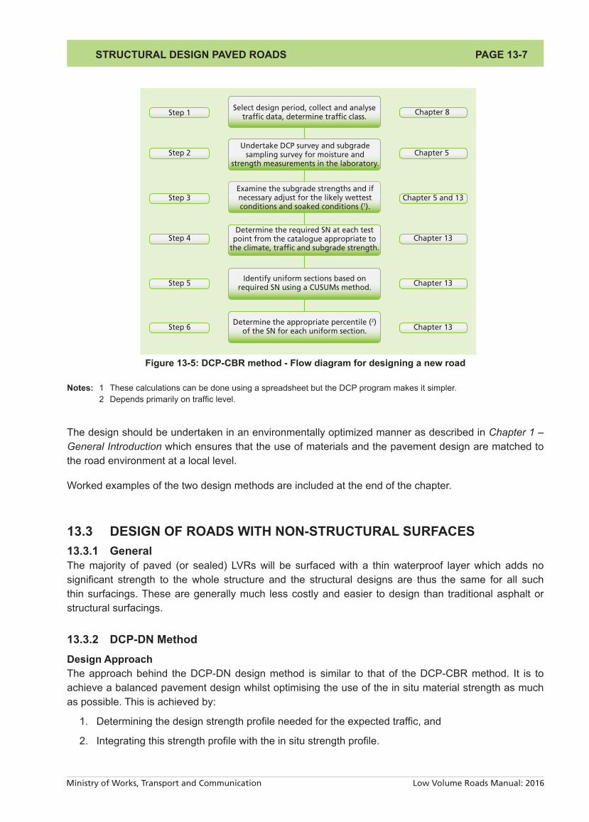
The flow diagram for new road design is shown in Figure 13-5.




Undertake a DCP survey plus a sampling survey for moisture and strength measurements in the laboratory.

For each test point determine the layer strength diagram (DN in mm/blow versus

depth and CBR versus depth) and the layer boundaries using the computer

program (1).

Determine the in situ SN values for each layer and the total SN (and SNP) for the pavement at each test point using the

DCP program (1, 2).

Convert the CBR values (and hence the SN values) from in situ to soaked

conditions for comparison with the design catalogue.

Determine the required SN values at each test point from the catalogue

appropriate to the climate, traffic and subgrade strength.

Compare the in situ with the required SN to determine the structural deficiency at each test point.

Identify uniform sections based on the structural deficiencies at each test point

using a CUSUM method.

Identify areas (a) where the structural deficiency is large and (b) areas where

layers are very weak and unlikely to meet the specifications for the layer that they will become in the upgraded design (3).

Determine the appropriate percentile (4) of the structural deficiencies for each

uniform section and design the upgrading requirements in terms of

additional layers and/or layer processing.

Step 1 Chapter 8

Chapter 5

Chapter 5 and 13

Chapter 13

Chapter 13

Chapter 13

Chapter 13

Chapter 13

Chapter 7 and13

Chapter 13

Step 2

Step 3

Step 4

Step 5

Step 6

Step 7

Step 8

Step 9

Step 10

Figure 13-4: DCP-CBR method - Flow diagram for upgrading an existing road

Notes: 1 These calculations can be done by hand using a spreadsheet but the UK DCP 3.1 program makes this easy and straightforward. 2 The SNP values are useful when the subbase and/or subgrade comprise a number of different layers of varying strengths. 3 Areas with material that does not meet the specifications for the layers that they will normally become in the upgraded design will require some form of reconstruction (or additional strengthening layers to increase the depth of the inadequate layers in the new pavement). 4 Depends primarily on traffic level.




Undertake DCP survey and subgrade sampling survey for moisture and

strength measurements in the laboratory.

Examine the subgrade strengths and if necessary adjust for the likely wettest conditions and soaked conditions (1).

Determine the required SN at each test point from the catalogue appropriate to

the climate, traffic and subgrade strength.

Identify uniform sections based on required SN using a CUSUMs method.

Determine the appropriate percentile (2) of the SN for each uniform section.

Step 1 Chapter 8

Chapter 5

Chapter 5 and 13

Chapter 13

Chapter 13

Chapter 13

Step 2

Step 3

Step 4

Step 5

Step 6

Notes: 1 These calculations can be done using a spreadsheet but the DCP program makes it simpler. 2 Depends primarily on traffic level.

The design should be undertaken in an environmentally optimized manner as described in Chapter 1 ‒ General Introduction which ensures that the use of materials and the pavement design are matched to the road environment at a local level.

Worked examples of the two design methods are included at the end of the chapter.

13.3 DESIGN OF ROADS WITH NON-STRUCTURAL SURFACES13.3.1 GeneralThe majority of paved (or sealed) LVRs will be surfaced with a thin waterproof layer which adds no significant strength to the whole structure and the structural designs are thus the same for all such thin surfacings. These are generally much less costly and easier to design than traditional asphalt or structural surfacings.

13.3.2 DCP-DN MethodDesign Approach The approach behind the DCP-DN design method is similar to that of the DCP-CBR method. It is to achieve a balanced pavement design whilst optimising the use of the in situ material strength as much as possible. This is achieved by:

1. Determining the design strength profile needed for the expected traffic, and

2. Integrating this strength profile with the in situ strength profile.

Figure 13-5: DCP-CBR method - Flow diagram for designing a new road



To use the existing gravel/earth road strength that has been developed over the years, the materials in the pavement structure need to be tested for their actual in situ strength, using a DCP as described in Chapter 5 ‒ Site Investigations. The result of each DCP test is a diagram of the strength of the existing pavement measured as DN values as a function of depth as illustrated in Figure 13-6.

The rate of penetration is a function of the in situ shear strength of the material at the in situ moisture content and density of the pavement layers at the time of testing, as described in Chapter 5 ‒ Site Investigations. However, most methods of pavement design require an estimate of the values of strength that would be obtained under the worst possible conditions: hence it is always recommended that DCP testing is done at the height of the wet season. If this cannot be achieved, the method of adjustment described in Section 13.3.4 can be used.

Useful parameters derived from the DCP analysis are the number of blows DN150 required to penetrate the top 150 mm of the pavement and the number of blows required to penetrate from 150 mm to 300 mm. These are the areas of the pavement that need to be the strongest and hence these parameters provide a quick appreciation of the likely need for strengthening and are also useful for delineating uniform sections. The DN800 is the total number of blows required for the DCP to penetrate to 800 mm and gives a broad measure of overall strength of the pavement somewhat analogous to the AASHTO Structural Number.

The analysis procedure for the DCP-DN method is different to that used in the DCP-CBR method and is described below.

Design Procedure The main elements are summarised in the flow diagram, Figure 13-3. The details from other chapters are not repeated here, thus Steps 1 to 5 and part of Step 6 are assumed to have been completed.

0

100

200

300

400

500

600

700

800

DN (mm)/blow)1 3 10 30

PEN

ETR

ATI

ON

DEP

TH (

mm

)

Figure 13-6: Typical DN with depth profile



Step 6 Determining the in situ layer strength profile for each uniform section: This is based on an “average analysis” for each uniform section as undertaken by the computer program (AFCAP DCP), which uses the data from all of the DCP profiles included in that uniform section. The layer strength (DN) profiles for each uniform section are plotted as shown in Figure 13-7 (all data) and Figure 13-8 (average, maxima and minima). Various percentiles of the layer strengths (DN values) to be used in the design process can be selected in the program and are computed automatically. Manual selection is based on the expected moisture conditions as discussed previously and summarized in Table 13-2.

Table 13-2: Suggested percentile of in situ DCP penetration rates to be usedSite moisture condition during

DCP surveyPercentile of strength profile (maximum penetration rate – DN)

Materials with strengths not moisture sensitive*

Materials with strengths that are moisture sensitive*

Wetter than expected in serviceExpected in service moistureDrier than expected in service

205080

20 – 5050 – 8080 - 90

* Moisture sensitivity can be estimated by inspecting and feeling a sample of the material – clayey materials (PI > about 12%) can be considered to be moisture sensitive. This can be confirmed by moisture test results.

The required layer strength profile for each uniform section is determined from the DCP design catalogue which is shown in Table 13-3 and illustrated in Figure 13-10 for different traffic categories.

The design catalogue is based on the anticipated, long term, in-service moisture condition. If there is a risk of prolonged moisture ingress into the road pavement, then the pavement design should be based on the soaked or a selected wetter condition. The DN value for any selected in situ moisture condition can be estimated from Table 13-4. This should be used as a guide only and testing of the actual materials involved should preferably be carried out. The values shown in Table 13-4 can be highly material dependent, especially for moisture sensitive materials and certain other materials such as laterites and calcretes.

LAYER-STRENGTH DIAGRAMDN (mm/blow)

PEN

ETR

ATI

ON

DEP

TH (

mm

)

0

200

400

600

800

1 3 10 30

LAYER-STRENGTH DIAGRAMDN (mm/blow)

PEN

ETR

ATI

ON

DEP

TH (

mm

)

0

200

400

600

800

1 3 10 30

Maximum

Average

Minimum

Figure 13-7: Collective strength profile for a uniform section

Figure 13-8: Average & extreme DCP strength profiles for a uniform section



Table 13-3: DCP design catalogue for different traffic classesTraffic Class

mesaTLC 0.01

0.003-0.01TLC 0.030.01-0.03

TLC 0.10.03-0.10

TLC 0.30.1-0.3

TLC 0.70.3-0.7

TLC 1.00.7-1.0

0- 150 mm Base≥ 98% Mod. AASHTO

DN ≤ 8 DN ≤ 5.9 DN ≤ 4 DN ≤ 3.2 DN ≤ 2.6 DN ≤ 2.5

150-300 mm Subbase≥ 95% Mod. AASHTO

DN ≤ 19 DN ≤ 14 DN ≤ 9 DN ≤ 6 DN ≤ 4.6 DN ≤ 4.0

300-450 mm Subgrade≥ 95% Mod. AASHTO

DN ≤ 33 DN ≤ 25 DN ≤ 19 DN ≤ 12 DN ≤ 8 DN ≤ 6

450-600 mmIn situ material

DN ≤ 40 DN ≤ 33 DN ≤ 25 DN ≤ 19 DN ≤ 14 DN ≤ 13

600-800 mmIn situ material

DN ≤ 50 DN ≤ 40 DN ≤ 39 DN ≤ 25 DN ≤ 24 DN ≤ 23

DSN 800 ≥ 39 ≥ 52 ≥ 73 ≥ 100 ≥ 128 ≥ 143

DSN800 is DCP structural number (i.e. number of blows required to reach a depth of 800 mm.

0

100

200

300

400

500

600

700

800

1 10 100

Dep

th (

mm

)

DN (mm/blow)

TLC0.01 (0.003 - 0.010) TLC0.03 (0.010 - 0.030) TLC0.1 (0.030 - 0.100)

TLC0.3 (0.100 - 0.300) TLC0.7 (0.300 - 0.700) TLC1.0 (0.700 - 1.000)

Figure 13-9: Layer strength profile for various traffic classes



Table 13-4: Relationship between standard soaked DN values and in situ DN at various moisture contents for different material strengths (CBR)

SoakedDCP DNvalue

mm/blowSoaked

CBR

Field DCP-DN (mm/blow)

Subgrade Base, subbase and selected layers

Wetclimate

Dryclimate

Very drystate

Dry state Moderatestate

Dampstate

3.62 80 1.43 1.73 2.19 3.13

4.54 60 1.65 2 2.5 3.6

5.69 45 1.85 2.23 2.84 4.07

7.84 7 2.15 2.55 3.25 4.7

9.04 25 4.79 4.21 2.25 2.72 3.45 4.93

13.5 15 5.08 4.42 2.58 3.1 4 5.75

18.6 10 6.37 5.59 3.01 3.62 4.6 6.64

24.6 7 6.5 5.79

48 3 6.94 6.12Notes: Moisture contents are expressed as ratios of in situ to Mod AASHTO optimum moisture contents as follows: Very dry = 0.25; Dry = 0.5; Moderate = 0.75; Damp = 1.0. This Table is only a guide and should be used with discretion. Materials that are highly moisture sensitive may produce different results.

Step 7: The representative in situ strength profiles are now compared with the required strength profile. The required strength profile is plotted on the same layer-strength diagram on which the uniform section layer strength profiles were plotted as illustrated in Figure 13-10. The comparison between the in situ strength profile and the required design strength profile allows the adequacy of the various pavement layers with depth to be assessed for carrying the expected future traffic loading.

0

100

200

300

400

500

600

700

800

Required strength profile (From DCP Design Catalogue)

In situ strength profile20th, 50th or 80th percentile as appropritae

Inadequatein situstrength

Adequatein situstrength

1 3 10 30DN (mm)/blow)

Dep

th (

mm

)

Figure 13-10: Comparison of required and in situ strength profiles



Step 8. Determining the upgrading requirements. Two options may be considered, as follows:Option 1: If the in situ strength profile of the existing gravel road complies with the required strength profile indicated by the DCP catalogue for the particular traffic class, the road would need to be only re-shaped, compacted and surfaced (assuming that the existing road is adequately above natural ground level to permit the necessary drainage requirements).

Option 2: If the in situ strength profile of the existing gravel road does not comply with the required strength profile indicated by the DCP catalogue for the particular traffic class (as is the case in the upper 150 mm of Figure 13-10), then the upper pavement layer(s) would need to be:

● Reworked- if only the density is inadequate and the required DN value can be obtained at the specified construction density and anticipated in-service moisture content.

● Overlaid – if the material quality (DN value at the specified construction density and anticipated in-service moisture content) is inadequate, then appropriate quality material will need to be imported to serve as the new upper pavement layer(s).

● Mechanically stabilized – as above, but new, better quality material is blended with the existing material to improve the overall quality of the layer

● Augmented – if the material quality (DN value) is adequate but the layer thickness is inadequate, then imported material of appropriate quality will need to be imported to make up the required thickness prior to compaction.

If none of the above options produces the required quality of material, recourse may be made to more expensive options, such as soil stabilisation. However, the design and construction requirements of stabilised layers is outside the scope of this Manual which focuses on the use of natural, untreated, materials. Reference may be made to other texts on the subject of stabilisation, such as the Pavement and Materials Design Manual, (MOW, 1999 - Chapter 7 ‒ Construction Materials) which deals with cemented materials. A fully worked example of the design DCP-DN method is included in Section 13.6.

13.3.3 DCP-CBR Method for New RoadsThe approach behind the DCP-CBR design method is similar to that of the DCP-DN method, i.e. to achieve a balanced pavement design whilst optimising the use of the in situ material strength as far as possible. The method is based on DCP test results but goes through a process of converting them to CBR values and then defining the pavement structure based on a structural number concept. For roads with non-structural bituminous surfacings the design charts shown in Tables 13-5 and 13-6 are utilised.

The subgrade is classified using the standard soaked CBR test to provide a strength index. It is not expected that the subgrades will become soaked in service except in exceptional circumstances and so the design catalogues show different thickness designs based on climate and drainage conditions for the same indexed subgrade class. A standard soaked CBR test is also used to evaluate the strength of the imported pavement materials.

Two design catalogues (charts) are used and two climatic zones are defined. The use of each chart also depends on the drainage and sealing provisions and the available materials as described below.



Wet climatic zoneIn the wet climatic zone, the following situations and solutions apply:

(a) Where the total sealed surface is 8 m or less, Pavement Design Chart 1 (Table 13-5) should be used. No adjustments to the roadbase material requirements are required.

(b) Where the total sealed surface is 8 m or more, Pavement Design Chart 2 (Table 13-6) should be used. The limit on the plasticity modulus of the roadbase may be increased by 20%. (refer to Figure 13-11 and Table 7-9, Chapter 7 ‒ Construction Materials).

(c) Where the total sealed surface is less than 8 m but the pavement is on an embankment in excess of 1.2 m in height, Pavement Design Chart 2 (Table 13-6) should be used. The limit on the plasticity modulus of the road base may be increased by 20%. (refer to Figure 13-11 and Table 7-9, Chapter 7 ‒ Construction Materials).

If the design engineer deems that other risk factors (e.g. poor maintenance and/or construction quality) are high, then Pavement Design Chart 1 should be used.

Moderate and dry climatic zoneIn a moderate or dry climatic zone Pavement Design Chart 2 (Table 13-6) should be used.

(a) Where the total sealed surface is less than 8 m, the limit on the plasticity modulus of the road base may be increased by 40%. (refer to Figure 13-11 and Table 7-9, Chapter 7 ‒ Construction Materials.

(b) Where the total sealed surface is over 8 m and when the pavement is on an embankment in excess of 1.2 m in height, the plasticity modulus of the road base may be increased by up to 40% and the plasticity index by 3 units. (refer to Figure 13-11 and Table 7-9, Chapter 7 ‒ Construction Materials).

Sealed width<8m

Sealed width>8m or 7m on

embankments > 1.2 mhigh

Sealed width>8m or 7m on

embankments > 1.2 mhigh

Moderate and Dry

Sealed width< 8m

DESIGN CHART 1

Materials relaxation.None allowed

Materials relaxation.Increase limit on PM

by 20%

Materials relaxation.Increase limit on PM

by 40%

Materials relaxation.Increase limit on PMby 40% and PI by 3

units

DESIGN CHART 2 DESIGN CHART 2 DESIGN CHART 2

Wet

Climate

Figure 13-11: DCP-CBR pavement design flow chart



Table 13-5: Bituminous pavement design Chart 1 (wet areas)

Subgrade CBRTLC 0.01 TLC 0.1 TLC 0.3 TLC 0.5 TLC 1.0

< 0.01 0.01 – 0.1 0.1 – 0.3 0.3 – 0.5 0.5 – 1.0

S1 (<3%) Special subgrade treatment required

S2 (3-4%) 150 G45150 G15

150 G65125 G30150 G15

150 G80150 G30175 G15

175 G80150 G30175 G15

200 G80175 G30175 G15

S3 (5-7%) 125 G45150 G15

150 G65100 G30100 G15

150 G65150 G30125 G15

175 G65150 G30125 G15

200 G80150 G30150 G15

S4 (8-14%) 200 G45 150 G65125 G30

150 G65200 G30

175 G65200 G30

175 G80150 G30

S5 (15-29%) 175 G45 125 G65100 G30

150 G65125 G30

150 G65150 G30

175 G80150 G30

S6 (>30%) 150 G45 150 G65 175 G65 200 G65 200 G80

Table 13-6: Bituminous pavement design Chart 2 (moderate and dry areas)

Subgrade CBRTLC 0.01 TLC 0.1 TLC 0.3 TLC 0.5 TLC 1.0

< 0.01 0.01-0.1 0.1-0.3 0.3-0.5 0.5-1.0


S2 (3-4%) 150 G45150 G15

150 G65125 G30150 G15

150 G80150 G30175 G15

175 G80150 G30175 G15

200 G80175 G30175 G15

S3 (5-7%) 125 G45125 G15

150 G55175 G30

175 G65175 G30

175 G80200 G30

175 G80250 G30

S4 (8-14%) 200 G45 150 G55100 G30

150 G55150 G30

175 G65150 G30

175 G80175 G30

S5 (15-29%) 150 G45 200 G55 125 G55125 G30

125 G65125 G30

150 G80125 G30

S6 (>30%) 150 G45 175 G45 175 G55 175 G65 175 G80

Once the quality of the available materials and haul distances are known, the flow chart in Figure 13-11 and the design charts can be used to review the most economical designs.

When the project is located close to the boundary between the two climatic zones, the wetter value should be used to reduce risks. When the design is close to the borderline between two traffic design classes, and in the absence of more reliable data, the next highest design class should be used.

The design charts do not cater for weak subgrades (CBR < 3%) and other problem soils, which will need specialist input and design, typically requiring imported, better quality, selected subgrade materials.

13.3.4 DCP-CBR Method for Upgrading an Existing RoadDesign approachThe DCP survey provides the thicknesses and in situ strengths of the layers of the existing road along the entire alignment. The analysis of the DCP data, preferably using the TRL DCP program, provides the overall strength of the pavement at each test point based on the structural number approach. The flow diagram is shown in Figure 13-5.



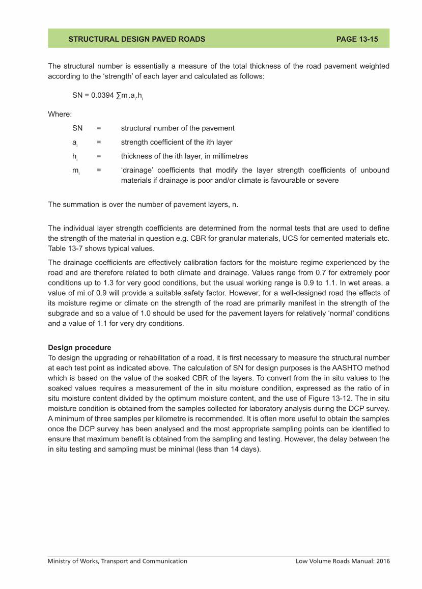
The structural number is essentially a measure of the total thickness of the road pavement weighted according to the ‘strength’ of each layer and calculated as follows:

SN = 0.0394 ∑mi.ai.hi

Where:

SN = structural number of the pavement

ai = strength coefficient of the ith layer

hi = thickness of the ith layer, in millimetres

mi = ‘drainage’ coefficients that modify the layer strength coefficients of unbound materials if drainage is poor and/or climate is favourable or severe

The summation is over the number of pavement layers, n.

The individual layer strength coefficients are determined from the normal tests that are used to define the strength of the material in question e.g. CBR for granular materials, UCS for cemented materials etc. Table 13-7 shows typical values.

The drainage coefficients are effectively calibration factors for the moisture regime experienced by the road and are therefore related to both climate and drainage. Values range from 0.7 for extremely poor conditions up to 1.3 for very good conditions, but the usual working range is 0.9 to 1.1. In wet areas, a value of mi of 0.9 will provide a suitable safety factor. However, for a well-designed road the effects of its moisture regime or climate on the strength of the road are primarily manifest in the strength of the subgrade and so a value of 1.0 should be used for the pavement layers for relatively ‘normal’ conditions and a value of 1.1 for very dry conditions.

Design procedureTo design the upgrading or rehabilitation of a road, it is first necessary to measure the structural number at each test point as indicated above. The calculation of SN for design purposes is the AASHTO method which is based on the value of the soaked CBR of the layers. To convert from the in situ values to the soaked values requires a measurement of the in situ moisture condition, expressed as the ratio of in situ moisture content divided by the optimum moisture content, and the use of Figure 13-12. The in situ moisture condition is obtained from the samples collected for laboratory analysis during the DCP survey. A minimum of three samples per kilometre is recommended. It is often more useful to obtain the samples once the DCP survey has been analysed and the most appropriate sampling points can be identified to ensure that maximum benefit is obtained from the sampling and testing. However, the delay between the in situ testing and sampling must be minimal (less than 14 days).



The relationship between soaked and in situ strength (CBR) depends on the characteristics of the materials. However, for the level of accuracy required, Figure 13-12, which is based on extensive research, is adequate. It should be noted that the comments regarding moisture sensitivity of some materials explained for Table 13-4 are equally applicable to Figure 13-12.

CBRs at different moisture contents

0.7 OMC

0.75 OMC

0.8 OMC

0.9 OMC

OMC

180

160

140

120

100

80

60

40

20

00 10 20 30 40 50 60 70 80 90

Soaked CBR

CB

R a

t o

ther

MC

s

Figure 13-12: CBRs at different moisture contents



Table 13-7: Pavement layer strength coefficientsLayer Type Condition Coefficient

Surface treatment ai = 0.2

Granular unbound roadbase

Default ai = (29.14 CBR - 0.1977 CBR2 +0.00045 CBR3) 10-4

CBR > 100% ai = 0.145

CBR = 100% ai = 0.14

CBR = 80% With a stabilised layer underneath With an unbound granular layer underneath

ai = 0.135

ai = 0.13

CBR = 65% ai = 0.12

CBR = 55% ai = 0.107

CBR = 45% ai = 0.1

Bitumen treated gravels and sands

Marshall stability = 2.5 MN ai = 0.135



Cemented

Equation ai = 0.075 + 0.039 (UCS) – 0.00088(UCS)2

CB 1 (UCS = 3.0 – 6.0 MPa) ai = 0.185

CB 2 (UCS = 1.5 – 3.0 MPa) ai = 0.23

Granular unbound subbases

Equation aj = -0.075 + 0.184 (log10 CBR) – 0.0444 (log10 CBR)2

CBR = 40% ai = 0.11

CBR = 30% ai = 0.1

CBR = 20% ai = 0.09

CBR = 15% ai = 0.08

CBR = 10% ai = 0.065

Cemented (UCS = 0.7 – 1.5 MPa) ai = 0.1Note: Unconfined Compressive Strength (UCS) is stated in MPa at 14 days.

Modified Structural NumberThe effect of different subgrades can also be included in the structural number approach. The subgrade contribution is defined as follows:

SNC = SN + 3.51 (log10 CBRs) – 0.85 (log10 CBRs)2 – 1.43

Where:

SNC = Modified structural number of the pavement

CBRs = In-situ CBR of the subgrade

The modified structural number (SNC) has been used extensively over the past 20 or 30 years and forms the basis for defining pavement strength in many pavement performance models. It should be used to identify the overall strength of each DCP test point in the old road if the subgrade is particularly variable.



Target Structural Numbers: When designing upgrading or rehabilitation it is necessary to determine the existing effective SN as described above at each test point and the required SN to carry the new design traffic. Table 13-8 to Table 13-11 show the target values of SN and SNC for different subgrade conditions and for different traffic levels calculated from the design charts for roads with a thin bituminous surfacing. The difference between the required structural number and the existing structural number is the deficiency that needs to be corrected.

The final step is to determine uniform sections based on the strengthening requirements using a CUSUM method. For each uniform section the following percentiles of the strengthening requirements should be used:

1. Median for TLC 0.01 and TLC 0.1

2. Upper 75 percentile for TLC 0.3

3. Upper 90 percentile for TLC 0.5 and TLC 1.0

However, when the strengthening requirements are large it may be more cost effective to carry out some reconstruction and, conversely if they are small, maintenance may be all that is required. Table 13-12 is a guide to the treatments.

Table 13-8: Structural Numbers (SN) for Bituminous Pavement Design Chart 1 (Table 13-4: Wet areas)Subgrade Class

(CBR)TLC 0.01 TLC 0.1 TLC 0.3 TLC 0.5 TLC 1.0

< 0.01 0.01 – 0.1 0.1 – 0.3 0.3 – 0.5 0.5 – 1.0


S2 (3-4%) 1.05 1.7 1.95 2.05 2.30

S3 (5-7%) 0.95 1.45 1.70 1.85 2.1

S4 (8-14%) 0.8 1.25 1.55 1.65 1.85

S5 (15-29%) 0.7 1.0 1.25 1.35 1.5

S6 (>30%) 0.6 0.7 0.85 0.95 1.0Note: These values exclude a contribution from the surfacing.

Table 13-9: Structural Numbers (SN) for Bituminous Pavement Design Chart 2 (Table 13-5: Moderate & Dry areas)

Subgrade Class (CBR)

TLC 0.01 TLC 0.1 TLC 0.3 TLC 0.5 TLC 1.0

< 0.01 0.01 – 0.1 0.1 – 0.3 0.3 – 0.5 0.5 – 1.0


S2 (3-4%) 1.05 1.55 1.80 2.0 2.15

S3 (5-7%) 0.9 1.35 1.55 1.70 1.95

S4 (8-14%) 0.7 1.05 1.35 1.45 1.6

S5 (15-29%) 0.6 0.85 1.05 1.1 1.3Note: These values exclude a contribution from the surfacing.

Table 13-10: Required Modified Structural Numbers (SNC) for Chart 1 (Table 13-4: Wet areas)Subgrade Class


S2 (3-4%) 1.1 1.75 2.0 2.1 2.35S3 (5-7%) 1.55 2.05 2.35 2.45 2.7S4 (8-14%) 1.85 2.25 2.6 2.7 2.9S5 (15-29%) 2.2 2.55 2.75 2.9 3.05S6 (>30%) 2.5 2.6 2.75 2.85 2.9



Table 13-11: Required Modified Structural Numbers (SNC) for Chart 2 (Table 13-5: Moderate & Dry areas)Subgrade Class


S2 (3-4%) 1.1 1.6 1.85 2.05 2.2

S3 (5-7%) 1.5 1.95 2.15 2.35 2.55

S4 (8-14%) 1.75 2.1 2.4 2.5 2.65

S5 (15-29%) 2.1 2.35 2.55 2.65 2.8

S6 (>30%) 2.5 2.6 2.65 2.75 2.8

Table 13-12: Structural Deficiency CriteriaStructural deficiency based on appropriate

percentilesAction Notes

0.2 or negative Maintain with a surface treatment (e.g. a surface dressing).

A thin granular overlay can be used to correct other road defects.

0.2 – 1.2 New granular layer. The existing layers must be checked for quality (subbase or roadbase). The minimum thickness of new roadbase should be 50 mm.

Some localised remedial works can be expected. A surface treatment is required.

1.2 – 1.8 The existing roadbase is likely to be only of subbase quality and should be checked. Additional subbase and a new roadbase are required.

Some localised remedial works will be needed. A surface treatment is required.

> 1.8 The existing layers are likely to be less than subbase quality, hence a new subbase and roadbase are required. Chemically stabilising existing material should be considered.

Localised remedial treatment and a surface treatment are required.

13.4 DESIGN OF ROADS WITH NON DISCRETE SURFACES13.4.1 GeneralStructural surfaces may have a place for use on LVRs. Initial cost is usually a constraining factor but the whole life costs may sometimes make these options favourable. The most common use is for semi-urban areas where marketing and trading takes place and where vehicle movements are unpredictable and on sections that are very steep or otherwise difficult from an engineering point of view.

13.4.2 Un-reinforced Concrete (URC)The un-reinforced cement concrete option for LVRs involves casting slabs 4.0 to 5.0 m in length between formwork with load transfer dowels between them. The thickness of the concrete depends on the traffic and subgrade support as shown in Table 13-13. In some cases, where continuity of traffic demands it, these slabs may be half carriageway width.



Table 13-13: Thickness (mm) – Un-reinforced concrete pavement (URC)Subgrade Class

(CBRTLC 01 TLC 0.1 TLC 0.3 TLC 0.5 TLC 1.0

< 01 0.01-0.1 0.1-0.3 0.3-0.5 0.5-1.0

S2 (3-4%)160 URC 170 URC 175 URC 180 URC 190 URC

150 G30 150 G30 150 G30 150 G30 150 G30


125 G30 125 G30 125 G30 125 G30 125 G30


100 G30 100 G30 100 G30 100 G30 100 G30


100 G30 100 G30 100 G30 100 G30 100 G30

S6 (>30%) 150 URC 150 URC 160 URC 170 URC 180 URCNotes:1. Cube strength = 30 MPa at 28 days.2. On subgrades > 30%, the material should be scarified and re-compacted to ensure the depth of material of in situ CBR >30% is in agreement with the recommendations.

13.4.3 Concrete StripsConcrete strips are currently not commonly used in Tanzania but they are a viable solution where traffic volumes are very low (< about 30 vpd). The pavement thickness under discrete elements given in Table 13-15 is used for the design. It is important to ensure adequate support under the strips to prevent cracking and movement under load especially in conditions of high moisture.

The strips must be constructed of B20 class concrete. If heavy trucks are expected, mesh wire reinforcement shall be used and placed at 1/3 depth from the surface. The concrete strips shall be 0.5 m wide, 1.5 to 3.0 m (max) in length and 0.2 m in thickness. The distance from centre to centre shall be 1.0 m.

13.5 DESIGN OF ROADS WITH DISCRETE ELEMENT SURFACINGS13.5.1 GeneralDiscrete element surfaces for LVRs do not usually provide much structural strength in terms of load spreading because the interlock between the elements is poor. However such surfacings are very useful for areas of marketing and trading and some have the advantage that they can be uplifted and replaced if damage to the surfaces themselves occurs or if there is a need to repair the underlying layers because of soil movement and deformation.

13.5.2 Hand-packed Stone (HPS)HPS paving consists of a layer of large broken stone pieces (typically 150 mm to 300 mm thick) tightly packed together and wedged in place with smaller stone chips rammed by hand into the joints using hammers and steel rods. The remaining voids are filled with sand or gravel. A degree of interlock is achieved and has been assumed in the designs shown in Table 13-14. The structures also require a capping layer when the subgrade is weak and a conventional subbase of G30 material or stronger is required. A capping layer also provides a smooth stable platform to work on.

The HPS is normally bedded on a thin layer of sand (SBL). An edge restraint or kerb constructed, for example, of large or mortared stones improves durability and lateral stability.



Table 13-14: Thicknesses designs for Hand Packed Stone (HPS) pavement (mm)Subgrade Class

(CBR)TLC 01 TLC 0.1 TLC 0.3 TLC 0.5 TLC 1.0

< 01 0.01-0.1 0.1-0.3 0.3-0.5 0.5-1.0

S2 (3-4%)

150 HPS 200 HPS 200 HPS 250 HPS

NA50 SBL 50 SBL 50 SBL 50 SBL

175 G30 125 G30 150 G30 150 G30

150 G15 200 G15 200 G15

S3 (5-7%)

150 HPS 200 HPS 200 HPS 250 HPS


125 G30 200 G30 150 G30 150 G30

150 G15 150 G15

S4 (8-14%)

150 HPS 200 HPS 200 HPS 250 HPS


100 G30 150 G30 200 G30 200 G30

S5 (15-29%)

150 HPS 200 HPS 200 HPS 250 HPS


Note Note Note Note

S6 (>30%)

150 HPS 200 HPS 200 HPS 250 HPS


Note Note Note NoteNotes: 1. The capping layer of G15 material and the subbase layer of G30 material can be reduced in thickness if stronger material is available.2. The capping layer can be G10 provided it is laid 7% thicker.3. The subbase layers can be material stronger than G30 and laid to reduced thickness. 4. On subgrades > 15%, the material should be scarified and re-compacted to ensure the depth of material of in situ CBR >15%.

13.5.3 Pave or Stone SettsStone sett surfacing or Pavé consists of a layer of roughly cubic (100 mm) stone setts laid on a bed of sand or fine aggregate within mortared stone or concrete edge restraints. The individual stones should have at least one face that is fairly smooth to be the upper or surface face when placed. Each stone sett is adjusted with a small (mason’s) hammer and then tapped into position to the level of the surrounding stones. Sand or fine aggregate is brushed into the spaces between the stones and the layer is then compacted with a roller. Suitable structural designs are shown in Table 13-15.

13.5.4 Clay BricksFired Clay Bricks are the product of firing moulded blocks of silty clay. The road surfacing consists of a layer of edge-on engineering quality bricks within mortar bedded and jointed edge restraints, or kerbs, on each side of the pavement. The thickness designs are as shown in Table 13-15 for TLC 0.01 and TLC 0.1. Fired clay brick surfacings are not suitable for traffic classes above TLC 0.1.

13.5.5 Cobble Stones or Dressed Stone PavementsCobble or Dressed Stone surfacings are similar to Pave and consist of a layer of roughly rectangular dressed stones laid on a bed of sand or fine aggregate within mortared stone or concrete edge restraints. The individual stones should have at least one face that is fairly smooth to be the upper or surface face when placed. Each stone is adjusted with a small (mason’s) hammer and then tapped into position to the level of the surrounding stones. Sand or fine aggregates is brushed into the spaces between the stones and the layer then compacted with a roller. Cobble stones are generally 150 mm thick and dressed stones



generally 150-200 mm thick. These options are suited for homogeneous rock types that have inherent orthogonal stress patterns (such as granite) that allow for easy break of the fresh rock into the required shapes by labour-based means.

The thickness designs are given in Table 13-15 except that the thickness of the cobblestone is generally 150 mm.

Table 13-15: Thicknesses designs for various discrete element surfacings (DES) (mm)Subgrade Class

(CBRTLC 01 TLC 0.1 TLC 0.3 TLC 0.5 TLC 1.0

< 0.01 0.01-0.1 0.1-0.3 0.3-0.5 0.5-1.0

S2 (3-4%)

DES DES DES DES DES

25 SBL 25 SBL 25 SBL 25 SBL 25 SBL

100 G65 125 G65 150 G80 150 G80 150 G80

100 G30 150 G30 150 G30 175 G30 200 G30

100 G15 150 G15 175 G15 200 G15 200 G15

S3 (5-7%)

DES DES DES DES DES


125 G65 150 G65 125 G80 150 G80 150 G80

100 G30 175 G30 125 G30 150 G30 175 G30

150 G15 150 G15 175 G15

S4 (8-14%)

DES DES DES DES DES


150 G65 150 G65 150 G80 150 G80 175 G80

100 G30 150 G30 200 G30 225 G30

S5 (15-29%)

DES DES DES DES DES


125 G65 100 G65 125 G80 150 G80 150 G80

125 G30 125 G30 125 G30 150 G30

S6 (>30%)

DES DES DES DES DES


125 G65 150 G65 150 G80 150 G80 150 G80

Note Note Note NoteNotes: 1. The capping layer of G15 material and the subbase layer of G30 material can be reduced in thickness if stronger material is available. 2. The capping layer can be G10 provided it is laid 7% thicker.

13.5.6 Mortared optionsIn some circumstances (e.g. on slopes in high rainfall areas and subgrades susceptible to volumetric change) it may be advantageous to use mortared options for the discrete element surfacings. This can be done with Hand-packed Stone, Stone Setts (or Pavé), Cobblestone (or Dressed Stone), and Fired Clay Brick pavements. The construction procedure is largely the same as for the un-mortared options except that cement mortar is used instead of sand for bedding and joint filling. The behaviour of mortared pavements is different to that of sand-bedded pavements and is more analogous to a rigid pavement than a flexible one. There is, however, little formal guidance on mortared options, although empirical evidence indicates that inter-block cracking may occur. For this reason the option is currently only recommended for the lightest traffic divisions up to TLC 0.1. Hence, refer to Table 13-15 until further locally relevant evidence is available.



13.5.7 Concrete BlocksConcrete blocks are usually constructed on a cement-stabilised base. A 25-50 mm sand blanket should be placed on top of the cement-stabilised base to provide a cushion and a drainage layer. The blocks shall be made of B20 concrete. Interlocking blocks are recommended.

13.6 DESIGN EXAMPLE DCP-DN METHOD13.6.1 Design Problem

1. A new paved road is to be built on the alignment of an existing gravel road to carry a cumulative design traffic of 0.3 MESA.

2. A DCP survey was carried out in the intermediate season (i.e. expected in-service conditions) and the data were analysed using WinDCP5.1 (the predecessor of AFCAP DCP).

3. In all, 87 DCP tests were carried out, one every 100 m over the total length of the road of 8.6 km.

The following design procedure was followed:

Step 1: Each DCP test was analysed using WinDCP5.1 “single measurement analysis”. From the outputs (Figure 13-13), the DSN800, and weighted average DN values for the upper three 150 mm layers of each DCP test were determined.

Figure 13-13: Typical output of WinDCP5.1



Step 2: These results were then used to identify uniform sections using a cumulative sum technique. Prior to this all obvious outliers based on DSN800 (very high or very low) were removed from the dataset (14 readings out of 87). The majority of these were particularly high, probably the result of stones within the layer. It is important, however, to check on site the actual reasons for the very high or very low readings as far as possible. Removal of the outliers only results in a smoothing of the curves and does not affect the actual “change points”.

Figure 13-15 shows a part of the spreadsheet used to calculate the “cumulative sums” and Figures 13-16 and 13-17 plots of the CUSUM curves for the different parameters. The CUSUM for the DSN800 values is calculated by obtaining the average of all of the DSN800 values (Column D in Figure 13-15) and then subtracting this from each of the DSN800 values (column E). The results are then added together (Column F). These values are then plotted against distance.

It is clear from the plots of DSN800 and DN301-450 that there are significant changes in the support at about km 2.0 and km 7.0. The change at km 7.0 is also reflected in the DN150 and DN151-300 plots. It is thus possible to derive 3 distinct uniform sections from these plots – 0 – 2.0 km, 2.0 – 7.0 km and 7.0 -9.0 km.

0

100

200

300

400

500

600

700

800

Ave. 20/80th percentile

0.1 1 10 100

DN (mm/blow)

Pave

men

t d

epth

(m

m)

Figure 13-14: WinDCP5.1 plot of penetration with depth for Test 1 (0.1 km)



Figure 13-15: Part of the spreadsheet showing the CUSUM calculation

1500

1300

1100

900

700

500

300

100

-100

-3000.0 1.0 2.0 3.0 4.0 5.0 6.0 7.0 8.0 9.0

Distance (km)

CU

SUM

DSN800

Figure 13-16: Plot of the CUSUM versus distance for the DSN800 results



20

0

-20

-40

-60

-80

-1000.0 1.0 2.0 3.0 4.0 5.0 6.0 7.0 8.0 9.0

Distance (km)

CU

SUM

0 - 150 mm 151 - 300 mm 301 - 450 mm

Figure 13-17: Plot of the CUSUM versus distance for the DN150, DN151-300 and DN301-450 results

Step 3: The data for each of these uniform sections are then analysed individually. The outliers can be retained or removed and generally have little impact on the final result. It can be seen that by retaining the outliers, the average DN150 is 4.59 compared with a value of 4.34 obtained when they are excluded, as shown in Figures 13-18 and 13-19 respectively.

The data can be analysed using either the average point analysis function in WinDCP5.1 or using the spreadsheet developed for the CUSUM analysis. The layer strength diagram output of the WinDCP5.1 analysis is shown in Figure 13-18. It can easily be seen that the average (note that this is not the 50th percentile) and the range between the 20th and 80th percentiles is very small.

Figure 13-18: Output of “average points analysis” (WinDCP5.1) for uniform section 1 including all points



Figure 13-19: Output of “average points analysis” (WinDCP5.1) for uniform section 1 excluding “outliers”

The percentiles can be calculated equally easily on the initial spreadsheet using the Excel functionalities.

Step 4: The process is repeated for each of the uniform sections. The results for each uniform section are summarised in Table 13-16.

It is clear from the results that the upper layer in all cases is inadequate. A single design solution for Uniform sections 1 and 2 requires that the upper layer be improved. The material should be investigated as it is only marginally inferior to see if processing such as blending, better compaction or stone removal could improve its quality to the required specification. If not the layer should be overlaid with a new 150 mm layer of selected material.

0

100

200

300

400

500

600

700

800

Ave. 20/80th percentile

0.1 1 10 100

DN (mm/blow)

Pave

men

t d

epth

(m

m)

Figure 13-20: WinDCP5.1 plot of average analysis for uniform section 1



Table 13-16: Summarised DN values for each layer and uniform sectionDesign Spec. Uniform Section 1 Uniform Section 2 Uniform Section 3

class DN Uniform Section 3 km 2+000 - 7+000 km 7+000 - 8+600

LE 0.3 mm/bl 50th %-ile 50th %-ile 50th %-ile

0-150 mm 3.2 4.01 3.68 10.07

151-300 mm 6 3.46 3.66 7.68

301-450 mm 12 5.16 3.83 7.81

451-600 mm 19 6.88 3.89 8.96

601-800 mm 25 7.06 4.57 11.04

DSN800 100 198.00 237.00 109.00

Uniform section 3 on the other hand is particularly poor. Neither of the two upper 150 mm layers are adequate. The addition of a single 150 mm layer would not prove adequate and in this case, the upper 150 mm layer needs to be removed and discarded. The underlying layer (150 – 300 mm) should be assessed to see if it could be improved by blending or some other treatment. If not, this section of the road requires the addition of 300 mm of material after removal of the upper 150 mm.

This is clearly illustrated for Uniform section 1 by Figure 13-21, showing a comparison of the in situ layer strengths with the layer strengths required for the selected traffic category. The areas shaded green are adequate and the yellow area is deficient. It is interesting to note that although the 50th percentile was used in this example, both the 80th and 20th percentiles for all but the upper layer would have proved adequate. In the upper 150 mm layer, none of the percentiles would allow the material to be used in its current condition.

0

100

200

300

400

500

600

700

800

0.1 1 10 100

DN (mm/blow)

Pave

men

t d

epth

(m

m)

User Def. 1 traffic Ave. 20/80th percentile

Figure 13-21: Layer strength diagram showing material strengths and traffic requirements



13.7 DESIGN EXAMPLE DCP-CBR METHOD13.7.1 Design Problem

4. An old road needs to be upgraded to carry a cumulative design traffic loading of 0.3 MESA.

5. A DCP survey is carried out in the intermediate season. The data are analysed using the TRL DCP program.

6. Samples of each layer of the pavement are taken for laboratory testing.

7. The climatic zone is dry hence design Chart 2 in Table 13-5 and Table 13-8 are to be used.

13.7.2 Basic Analysis ProcedureThe following analysis is carried out for each DCP test point.

Step 1 Initial analysis of each DCP testA typical DCP result is shown in Figure 13-22. The program identifies the layer boundaries automatically and outputs, for each layer, the thickness, average mm/blow, and CBR. Usually more than one subbase layer is identified.

Step 2 Defining the pavement layers and computing pavement strengthThe user must define each layer as roadbase, subbase, or subgrade. The program then calculates the contribution of each layer to the overall structural number. The strength coefficients are calculated automatically (Table 13-17).

0

-100

-200

-300

-400

-500

-600

-700

-800

0 10 20 30 40 50 60 70

Subbase: 12.6 mm/blowCBR = 21%h = 315 mm

Subbase: 6.1 mm/blowCBR = 45%h = 160 mm

Subgrade: 27.5 mm/blowCBR = 9.1%

Dep

th in

mill

imet

res

Number of Blows

Figure 13-22: Typical DCP test result



Table 13-17: Example of CBRs, strength coefficients and SNs at a DCP test chainageLayer

NoCBR %

Thickness(mm)

Depth(mm)

PositionStrength

CoefficientSN

1 45 160 160 Roadbase 0.10 0.63

2 21 315 475 Subbase 0.09 1.12

9.1 - Subgrade

Total 475 1.75

Step 3 Adjustment for moisture conditionsThese SNs are the values obtained at the in situ conditions. For evaluation and design purposes the SN of each layer in the soaked condition is required. The user must estimate the soaked CBR values from the in situ moisture contents measured in laboratory tests of the samples. This is done using Figure 13-7. This conversion cannot be exact because the relationships shown in the Figure depend on various material properties such as PI, hence a high level of precision is not possible, and nor is it necessary. In this example the in situ conditions are not extreme (in terms of wet or dry). An average in situ moisture content of OMC was obtained and used with Figure 13-12 to convert the CBRs to soaked conditions.

The strength of the subgrade must also be adjusted to give an estimate of the soaked value. However, it is only necessary to identify the subgrade class. For low values of CBR, if the in situ moisture regime is OMC the soaked value is typically half to one third of the in situ value. If the moisture regime is dry (0.75*OMC) then the soaked value is one third to one quarter of the in situ value.

The revised CBRs are shown in Table 13-18. Using the revised CBR values, the revised SN is calculated for each layer and then summed to give the total value as shown in Table 13-18.

Table 13-18: Example of revised CBRs and SNs corrected for moisture at a DCP test chainageLayer

NoCBR (%)

Thickness(mm)

PositionRevised CBR

(%)Revised strength

coefficientRevised SN

1 45 160 Roadbase 20 0.09(1) 0.57

2 21 315 Subbase 5 0.03 0.37

9.1 - Subgrade

Total 475 0.94

Step 4 Estimation of strengthening requirementsHaving determined the subgrade strength and the existing SN for each of the DCP test points, design Chart 1 (Table 13-8 or 13-10) is used to determine the SN or SNC required for the new road to carry the design traffic on the design subgrade. The difference between the required SN and the existing SN (ΔSN) is the key parameter on which the upgrading design is based. The calculations are carried out for every test point remembering that the subgrade may not be the same for all the DCP test points.

The choice of using SN or SNC depends on the variability of the subgrade. SNC should be used if the subgrade is variable. Calculations can be done using both SN and SNC and the more conservative results used in the design.

Step 5 Defining the upgrading treatmentsThe results of the DCP testing and preliminary analysis using the DCP program is a graph showing the CUSUM calculations of structural deficiencies as a function of chainage along the road as shown in Figure 13-23. (Using the UK DCP 3.1 program, similar CUSUM calculations can be automatically generated for any of the parameters derived from the DCP tests if desired).



Changes in the slope of the trend line identify relatively homogenous or uniform sections. There are 3 sections that are distinct namely:

● Section 1 Chainage 0.000 to 3.600 where the road is generally thick but weak and not very uniform (little variation in fluctuating CUSUM).

● Section 2 Chainage 3.700 to 7.000 where the road is stronger and more uniform (steeply decreasing CUSUM).

● Section 3 Chainage 7.100 to 8.600 where the road is much weaker (increasing CUSUM).

Section 1In general the main problem in Section 1 is that out of 35 test points there are 21 with distinct roadbase problems, identified from a visual inspection of the individual DCP test results and/or the tables summarising the properties of each individual test that are computed automatically in the program. The problems are of one or more of three types.

1. Loose upper layer.

2. Weak middle layer.

3. Overall weakness in the road base.

A total of 14 of the test points require no treatment at all except surface smoothing and compacting but these points are distributed fairly evenly along the section with never more than two being adjacent to each other. It is not feasible to change the treatment at short intervals, even with labour based construction, because it is probably impossible to identify the boundaries. The variations along the road are frequent and probably largely random hence the sections of similar characteristics may be very short.

0.0 1.0 2.0 3.0 4.0 5.0 6.0 7.0 8.0 9.0

5.0

0.0

-5.0

-10.0

-15.0

-20.0

CUSUM on delta SNC

Shainage

CU

SUM

Figure 13-23: CUSUM analysis to identify uniform sections



The treatment for Type 1 is simply to test the top (roadbase) layer to see if it can be made strong enough by some sort of processing, for example, merely compaction or possibly blending.

The treatment of Type 2 is not so straightforward because it could be an internal drainage problem, but the weak layer is normally underneath a strong layer and is therefore quite deep. The true nature of the problem needs to be determined before any major processing is considered but it may simply require an additional surface layer to “push” the weak layer to a lower (subbase) level.

The treatment of Type 3 is the same as for Type 1 but the chances of getting a strong enough layer by blending and/or compaction are probably less.

In Section 1 there are just 6 DCP results that indicate that additional material may be needed simply because the existing SN is too low (in contrast to much of the Section where the existing material is deficient in quality but where the overall SN is high because of thickness). These are at chainages 0.6, 1.1, 2.0, 2.9, 3.1 and 3.5 and correspond to the lowest subgrade strengths. The CUSUM graph shows that these are identified by the large jump in the y-coordinate that occurs between the chainages mentioned and the preceding chainage. They appear to be isolated points so they may be associated with local drainage issues. Five of them are also associated with weak bases so could possibly be corrected by reprocessing the existing material. The 6th (at chainage 2.9) may require an additional layer of base material (100 mm) because the existing base is only 100 mm thick and the SN is marginal. A subsidiary investigation is needed to determine the extent of these six problems.

Figure 13-24 shows the thicknesses required at each test point. The chainages with no vertical bar do not need additional strengthening but, based on practical issues, the entire section, after the six weak sections have been re-examined, will require the same treatment.

Section 2Section 2 is much more uniform than Section 1, but 18 of the 34 test points show the same roadbase problems, as shown in Figure 13-25. There are 16 chainages that require no treatment but some of them (but not all) tend to occur slightly more often adjacent to one another in contrast to those in Section 1. For example chainages 4.0 to 4.2; 4.5 to 4.7; 6.8 to 7.0 but these sub-sections are also probably too short to warrant different treatment to that of the rest of the Section.

Section 1 (0.000 - 3.600)200

150

100

50

0 0 0.2 0.4 0.6 0.8 1 1.2 1.5 1.7 1.9 2.1 2.3 2.6 2.8 3 3.2 3.4 3.6

Chainage

New roadbase

Thic

knes

s o

f n

ew r

oad

bas

e (m

m)

Figure 13-24: Section 1: Potential requirements for additional roadbase for each DCP test.



Section 3The whole of Section 3 (16 DCP test points) also shows roadbase deficiencies including a complete absence of any roadbase or subbase at many of the test points, as illustrated in Figure 13-26. The subgrade is quite strong hence a relatively thin pavement is required. Most of the Section is founded on an S4 subgrade or stronger and, except for three chainages (7.1, 7.4 and 7.8) already has a sufficiently high SN. The reason why additional material is needed is that the uppermost layer (be it roadbase, subbase or simply the top of a strong subgrade) are too weak for their position in the pavement. An additional 150 mm layer of suitable material on all the test points is required for a TLC 0.3 MESA design and, on the 8 test points with no subbase, an addition subbase layer is required. However, it is not usually feasible to change designs frequently hence the whole section requires two additional layers of pavement. The weakest test point is at chainage 7.1 and corresponds to the weakest subgrade and could therefore also be a drainage problem that needs investigating separately before a design for this area can be chosen.

Section 2 (3.600 - 7.000)200

150

100

50

03.7 3.9 4.1 4.3 4.5 4.7 4.9 5.1 5.3 5.5 5.7 5.9 6.1 6.3 6.5 6.7 6.9

Chainage

New roadbase

Thic

knes

s o

f n

ew r

oad

bas

e (m

m)

Figure 13-25: Section 2: Potential requirements for additional roadbase for each DCP test

Section 3 (7.000 - 8.000)

Chainage

Thic

knes

s o

f n

ew r

oad

bas

e (m

m)

450

400

350

300

250

200

150

100

50

0 7.1 7.2 7.3 7.4 7.5 7.6 7.7 7.8 7.9 8 8.1 8.2 8.3 8.4 8.5 8.6

Capping

Subbase

Roadbase

Figure 13-26: Section 3: Potential requirements for additional roadbase and subbase for each DCP test point



All of this information has been obtained directly from the DCP profiles on a point by point basis.

Step 6 Design for each uniform sectionFor each uniform section there is a range of values of ΔSNs but this is much smaller now that the uniform sections have been defined. The next step is to choose the appropriate percentile of those ranges for design. The percentile depends on the reliability required; the recommended values (Section 13.3.3) are:

● Median for TLC 0.01 and TLC 0.1

● Upper 75th percentile for TLC 0.3

● Upper 90th percentile for TLC 0.5 and TLC 1.0

Thus for TLC 0.3 a 75th percentile is recommended but for this example there are only two different designs for two sections and only three for Section 3 hence the choice of percentile requires no calculation. A summary is shown in the Table 13-19.

Table 13-19: Results of the analysis for road class TLC 0.3Section 1 2 3

Chainage 0.000 – 3.600 3.600 – 7.000 7.000 – 8.600

Material to be added

150 mm of CBR 65%(1) 150 mm of CBR 65%(1)150 mm of CBR 65% and

200 mm of CBR 30%Note 1: Additional roadbase is needed only if the existing roadbase cannot be brought up to specified characteristics by other means, e.g. blending.Note 2: Chainages with possible drainage problems (see text) require further investigation.



BIBLIOGRAPHY

AFCAP (2016). AfCAP DCP analysis software. http://www.research4cap.org/SitePages/Research.aspx.

American Association of State Highway and Transportation Officials (1993). AASHTO Guide for Design of Pavement Structures. Washington, D.C., USA.

Committee of Land Transport Officials (COLTO) (1996). Structural Design of Flexible Pavements for Inter-urban and Rural Roads. Technical Recommendations for Highways, TRH4. Department of Transport, Pretoria, South Africa.

CSIR (2001). WinDCP 5.0 software. CSIR, Pretoria, South Africa.

De Beer M, Kleyn E G and P F Savage (1988). Towards a Classification System for the Strength-balance of Thin Surfaced Flexible Pavements. DRTT Report 637, CSIR, Pretoria, South Africa.

De Beer M (1989). Dynamic cone penetrometer (DCP)-aided evaluation of the behaviour of pavements with lightly cementitious layers. Research Report DPVT 37, CSIR, Pretoria, South Africa.

Emery S J (1985). Prediction of Moisture Content for Use in Pavement Design. PhD Thesis, Univ. of Witwatersrand, Johannesburg, South Africa.

Giummarra G (1995). Sealed local roads manual. ARRB Transport Research Ltd., Australia.

Gourley C S and P A K Greening (1999). Performances of low-volume sealed roads; results and recommendations from studies in southern Africa. TRL Published Report PR/OSC/167/99. TRL, UK. Crowthorne, Berkshire,UK.

Government of Malawi, Ministry of Transport and Public Works (2013). Design Manual for Low Volume Sealed Roads Using the DCP Design Method. Lilongwe, Malawi.

Kleyn E G and P F Savage (1982). The application of the pavement DCP to determine the bearing properties and performance of road pavements, Proc Int Symp on Bearing Capacity of Roads and Airfields, Trondheim, Norway, 1982.

Kleyn E G and G D van Zyl (1988). Application of the DCP to Light Pavement Design. First Int. Symposium on Penetration testing, Orlando, USA.

Kleyn E G (1982). Aspects of pavement evaluation and design as determined with the aid of the Dynamic Cone Penetrometer (DCP). M.Eng. Thesis, University of Pretoria, Pretoria.

Ministry of Works, Tanzania (1999). Pavement and Materials Design Manual. TANROADS, Dar es Salaam.

Mitchell R L, C P van der Merwe C P and H K Geel (1975). Standardised Flexible Pavement Design for Rural Roads with Light to Medium Traffic, Ministry of Roads and Road Traffic, Salisbury, Rhodesia.

Transport Research Laboratory (1993). Overseas Road Note 31. A guide to the structural design of bitumen-surfaced roads in tropical and sub-tropical climates. Overseas Centre, TRL, Crowthorne, Berkshire, UK. (4th edition).

Transport Research Laboratory (1993). Measuring Road Pavement Strength and Designing Low Volume Sealed Roads Using the Dynamic Cone Penetrometer. Unpublished Project Report UPR/IE/76/06. Project Record No. R7783. TRL Limited, Crowthorne, Berkshire, UK.

Transport Research Laboratory (1999). A guide to the pavement evaluation and maintenance of bitumen-surfaced roads in tropical and sub-tropical countries. Overseas Road Note 18. TRL Limited, Crowthorne, Berkshire,UK.



Transport Research Laboratory (2004). UK DCP version 2.2. TRL Limited, Crowthorne, Berkshire, UK.

Van der Merwe C P (1999). Material and Pavement Structures for Low Volume Roads in Zimbabwe. Unpublished Report, Harare.

Wolff H, S J Emery, van Zyl G D and P Paige-Green (1995). Design Catalogue for Low-Volume Roads Developed for South African Conditions. Proc. Sixth Int. Conf. on Low-Volume Roads, Proc. Sixth Int. Conf. on Low-Volume Roads, Minneapolis, Minnesota, USA.

37STRUCTURAL DESIGN UNPAVED ROADS









8. Traffic

9. Geometric Design

10: Road Safety





15: Surfacing





PART A:Introduction

PART B:Planning


PART D:Design

PART E:Construction


38 STRUCTURAL DESIGN UNPAVED ROADS


CONTENTS

14.1 INTRODUCTION ......................................................................................................................14-1 14.1.1 Background .................................................................................................................14-1 14.1.2 Purpose and Scope .....................................................................................................14-1

14.2. EARTH ROADS .......................................................................................................................14-2 14.2.1 General ........................................................................................................................ 14.2 14.2.1 Un-engioneered ...........................................................................................................14-2 14.2.2 Engineered ..................................................................................................................14-2

14.3. GRAVEL ROADS ....................................................................................................................14-4 14.3.1 General ........................................................................................................................14-4 14.3.2 Materials ......................................................................................................................14-5 14.3.3 Thickness Design ........................................................................................................14-6

14.4. TREATED GRAVEL ROADS ................................................................................................. 14-11

14.5. EXAMPLE OF DCP DESIGN METHOD ............................................................................... 14-11

BIBLIOGRAPHY ....................................................................................................................14-14

LIST OF TABLES Table 14-1: Specification requirements for wearing course materials for unpaved roads…14-5 Table 14-2: Suggested percentile of minimum in situ DCP penetration rates to be used ...14-8 Table 14-3: Thickness and strength design of support structures for different traffic categories (DN) ........................................................................14-9 Table 14-4: Typical estimates of gravel loss .....................................................................14-10 Table 14-5: Spreadsheet showing the CUSUM calculation ..............................................14-12 Table 14-6: Summary of percentile values for each parameter in each uniform section ..14-12 Table 14-7: Structural properties of each uniform section (tested in dry period) ...............14-13 Table 14-8: Structural properties of each uniform section (tested in wet period) ..............14-13

LIST OF FIGURES Figure 14-1: Hierarchy of roads showing unpaved and low volume sealed roads ...............14-1 Figure 14-2: Cross section of typical improved earth road ...................................................14-3 Figure 14-3: Carrying capacity of engineered earth roads ..................................................14-3 Figure 14-4: Chart showing performance of unpaved road materials ..................................14-5 Figure 14-5: Layer strength diagrams of support layers for different traffic categories ........14-9 Figure 14-6: Plot of CUSUMs for different parameters .......................................................14-12



14.1 INTRODUCTION14.1.1 BackgroundMore than 90% of the road network in Tanzania consists of unpaved roads. Although often rudimentary, these roads provide communities with access to important services (schools, clinics, hospitals and markets) and are the basis of a thriving market and social environment.

Unpaved roads are defined in this Manual as any road that is not surfaced with a “water proof” surfacing, whether this be bituminous, concrete, interlocking blocks, cobbles or similar surfacings.

In their simplest forms, unpaved roads consist of tracks or earth roads over which goods or persons are moved directly on the in situ material surface. This may in some cases be ripped, shaped and compacted (engineered) but generally the only compaction is that applied by vehicles moving over it (un-engineered).

There comes a point with these “roads” when passability is excessively affected by the weather and vehicles can no longer traverse the road during inclement weather. This problem is best solved by applying a selected material with specific properties over the in situ material to ensure all-weather passability and the roads then become “gravel” roads. Despite this the roads may occasionally become impassable as a result of flooding of parts of the road, in which case vehicles cannot pass because of deep water and not necessarily any reason attributed to the road surface.

Unpaved roads will usually carry a maximum of about 200 to 300 vehicles per day (with less than 10 % being heavy) but in areas where materials are poor, upgrading to paved standard can often be economically justified at traffic volumes much lower than this.

An example of the typical types of low volume road is shown in Figure 14-1.

14.1.2 Purpose and ScopeThe purpose of this chapter is to provide a framework for the design of unpaved roads in an economic and sustainable manner such that the appropriate levels of quality are produced. The chapter has been developed so as to harmonise with the relevant sections described in the Pavement and Materials Design Manual (MOW, 1999) as far as possible. Innovations have been introduced where considered appropriate.

Eart

h

Quality of Service

Co

nst

ruct

ion

co

st

Trac

k

Gra

vel

Surf

aced

Hig

hw

ay

Surf

aced

Sta

nd

ard

s

Wel

l des

ign

edEn

gin

eere

d G

rave

l

Seal

ed L

ow

Vo

lum

e R

oad

s

Trea

ted

Gra

vel R

oad

s

Wel

l mai

nta

ined

Eng

inee

red

Gra

vel

Figure 14-1: Hierarchy of roads showing unpaved and low volume sealed roads



The chapter covers the design of all levels of unpaved roads from earth roads making use of the in situ soil to engineered and treated gravel roads. Material selection and thickness design are treated in detail.

14.2 EARTH ROADS14.2.1 GeneralEarth roads may comprise either un-engineered roads on which traffic travels directly on the in situ material or engineered roads in which some attempt is made to improve the shape of the road, introduce side-drains and usually apply some compaction to the material. The wearing course material is generally obtained from excavation of the side-drains.

14.2.2 Un-engineeredUn-engineered roads usually start as one or two tracks in which the grass and surface vegetation is worn away to expose the in situ material or in some cases the vegetation may be intentionally removed. With time and traffic, these tend to wear down and depressions develop in the natural ground surface. These become areas that collect precipitation or surface run-off and form conduits moving the water, which leads to softening of the material, erosion and ultimately deepening of the channels. At this stage the tracks no longer afford viable routes for traffic and new tracks are formed adjacent to the existing ones, ultimately resulting in a wide “canal”.

The life and effectiveness of earth roads depends on the nature of the in situ material. Often the upper part has humus and clay, which results in some sort of binding of the material, which can be improved by the “reinforcing” effect of any roots. Once these wear away the track will usually deteriorate rapidly.

In some instances, the in situ material may have properties equivalent to those required for conventional wearing course gravels, in which case they may perform reasonably well for a limited period. It should be remembered that these materials are generally not compacted and rely solely on traffic compaction to increase their density, which is accompanied by settlement and some material loss.

Only once the earth road starts deteriorating in riding quality, is it graded and given some shape but the overall structure is usually below natural ground level and the associated drainage problems are not addressed. At this stage the road needs to be improved.

14.2.3 Engineered Engineered or improved earth roads differ from the un-engineered earth roads described above in that the shape of the road structure is improved. The materials used are the same as the earth road, i.e. the in situ or local material but additional material is excavated from the side of the road to form side drains (at least 150 mm below natural ground level) and this material is added to the road to increase its height and provide a better drained road structure, as shown in Figure 14-2.The material must be shaped to assist with water runoff and compacted to improve its strength, decrease its permeability and reduce maintenance requirements.

The crossfall of carriageway and shoulders for all engineered and gravel roads shall be 4 to 6% depending on local conditions, to prevent potholes developing by ensuring rapid removal of water from the road surface and to ensure that excessive crossfall does not cause erosion of the surface. Although a maximum of 5% is usually recommended, it is often useful to construct a camber of 6%, as 1% is usually lost soon after construction.



The crown height of the improved earth road should be at least 35 cm above the bed of the side drains, which must be graded and lead into regular side and mitre drains to remove water from adjacent to the road as rapidly as possible. The invert of the side drain should be at least 150 mm below the bottom of the wearing course.

The performance of earth roads is constrained by the quality of the in situ materials, which in many cases is inadequate to provide good all-weather surfaces that require minimal maintenance. A knowledge of the past performance of local materials may, however, allow the use of these even though they do not comply with the required properties for good wearing course gravels. In general, no specific material requirements are applicable to earth roads but if the local materials comply with the requirements for gravel roads, a good performance can be expected.

It is possible to estimate the likely performance of improved earth roads based on an assessment of the traffic carrying capacity of the soils under varying environmental conditions from a knowledge of the bearing capacity (CBR) of the soil, the equivalent single wheel load of the vehicles and the tyre pressures, as shown in Figure 14-3. If the strength of the earth road material is known (in terms of its in-situ CBR), the nomograph permits predictions of the expected number of vehicles that will cause a rut depth of 75 mm.

Side drain

35 cm 15 cm

Flat table drain is preferable when maintained manually

V-shaped drain is preferable when table maintained by grader

Figure 14-2: Cross section of typical improved earth road

1008060

40

20

108

6

4

2

1

CBR

Single or equivalent singlewheel load in kN

4.5

333

267222

179

134

9045

229

103 172 344 482 689 1033 1379 2060kPa

Tyre inflation pressure

10000800060004000

2000

1000800600400

200

100806040

20

10864

2

1

Coverages

Figure 14-3: Carrying capacity of engineered earth roads Source: Ahlvin and Hamitt (1975).



As illustrated in Figure 14-3, an engineered earth road with an in-situ CBR of 10% can be expected to provide approximately 2 000 coverages of vehicles with a single wheel load of 45 kN and a tyre inflation pressure of 482 kPa before serious deformation is likely to occur. Since the wheel loads will not be concentrated on exactly the same path, but will wander slightly across the width of a road, one complete coverage is equivalent to the passage of 2.7 vehicles. Thus, 2,000 coverages are equivalent to 5,400 vehicles with the characteristics indicated above.

For a single lane road, the wheel loads will be restricted to narrower channels and therefore the coverages will be different. For example, for a narrow single lane road the number of vehicles that the earth road can accommodate before failure decreases to approximately 1350 vehicles. For a route carrying 50 vpd and assuming 15% of them are relatively heavy (4.54 tonne wheels), this translates into a need to maintain, re-grade or reshape the surface about every 4 to 6 months. For soils with higher CBR this will be longer. It is important for both designers and road managers to appreciate that engineered earth roads have a low initial cost but that they require an ongoing commitment to regularly reshape the surface to keep it in a serviceable condition.

Areas that may have specific problems (usually due to water or to poor subgrade materials) may be treated in isolation, by localised replacement of subgrade, gravelling, installation of culverts, raising the roadway or by installing other drainage measures. This is the basis of a “spot improvement” approach and should be carried out to the best standard possible as these areas will then be in a condition that is suitable for later upgrading to gravel road standard.

Where the topography allows, wide, shallow longitudinal drainage for earth roads is preferred. These minimise erosion, and will not block as easily as narrow ditches. The ditches grass over in time, binding the soil surface and further slowing down the water flow speed, both of which act to prevent or reduce erosion.

Culverts should be installed perpendicular to the route where there is a need to transfer water from one side of the road to the other, for example where the road crosses a watercourse. In flat areas, smaller diameter parallel culverts may be preferable to single large culverts, in order to ensure discharge is at ground level. However, culvert pipes smaller than 750 mm in diameter are not recommended as they are difficult to clean out of silt and debris. The inlet and outlet of the culvert must be protected against erosion.

At some point (usually dictated by the number of vehicles increasing to a certain level and depending on the material quality) the maintenance requirements for earth roads reach a stage that it becomes uneconomical or excessively difficult. At this stage, a decision must be made to construct a traditional gravel road in which materials form a selected borrow source are used for the wearing course.

14.3 GRAVEL ROADS14.3.1 GeneralRoads described as gravel roads imply that a number of factors have been taken into account in their design and construction. These include:

● Material of a selected quality is used to provide an all-weather wearing course.

● The structure of the road and strength of the materials is such that the subgrade is protected from excessive strains under traffic loads.

● The shape of the road is designed to allow drainage of water (mainly precipitation) from the road surface and from alongside the road.

● he necessary cross and side drainage is installed.

● The road is constructed to acceptable standards, including shape, compaction and finish.



Although an all-weather wearing course is provided, the road may not necessarily be passable at all times of the years as a result of low level water crossings being flooded periodically. This, however, is not a function of the gravel roads design and is addressed under a different section of this Manual. (Chapter 11- Hydrology and Drainage Structures).

14.3.2 MaterialsThe critical aspect of gravel roads is obviously the material selection. The use of incorrect materials in the wearing course will result in roads that deform, corrugate, become slippery when wet, lose gravel rapidly and generate excessive dust. Table 14-1 summarises the required properties of good wearing course gravels and these are based on materials tested using the standard Tanzanian test methods.

Table 14-1: Specification requirements for wearing course materials for unpaved roadsMaximum nominal size Minimum percentage passing 37.5 mmShrinkage product (SP)Grading coefficient (Gc)Min DN value (mm/blow)Treton Impact value (%)1

37.5 mm95140 – 400 (260)14 – 3013.5 at 95% BS Heavy compaction (soaked) 20 – 65

Note 1: The Treton impact value is not a standard Tanzanian test but is described in TMH 1 (1985). It is a simple test and makes use of equipment that can be easily manufactured. No correlation currently exists with the similar BS Aggregate Impact Test.

The recommended grading and cohesion (shrinkage) specifications for gravel wearing course materials can also be shown diagrammatically in relation to their predicted performance, as shown in Figure 14-4.

0

50

100

150

200

250

300

350

400

450

500

0 2 4 6 8 10 12 14 16 18 20 22 24 26 28 30 32 34 36 38 40 42 44 46 48

Shri

nka

ge

Pro

du

ct

Grading Coefficient

DSlippery

AErodible

CRavels

EGood

BCorrugates and ravels

Figure 14-4: Chart showing performance of unpaved road materialsNote: Figure 14-4 is based on CML test methods. Should the results be determined using the CSIR Gravel Roads Test Kit (based on TMH 1 test methods), the chart provided with the kit should be used.



On the chart presented in Figure 14-4, the 5 zones indicated (A to E) show the expected performance of materials as follows:

● Zone A: Fine grained material prone to erosion.

● Zone B: Non-cohesive materials that lead to corrugation and ravelling/loosening.

● Zone C: Poorly graded materials that are prone to ravelling.

● Zone D: Fine plastic material prone to slipperiness and excessive dust.

● Zone E: Optimum materials for best performance.

Requirements for both material and aggregate strength are provided. The material strength is specified as the DCP DN value (13.5 mm/blow) which initially appears very low but investigation of many roads in various countries has shown that material with a strength as low as this will not shear or deform under the passage of an 80 kN axle load (20 kN single tyre load), even when soaked. Materials of significantly higher quality than this should be preserved for later use in paved roads. The Treton impact value differentiates between aggregate particles that will perform well (20 to 65), aggregates that are too soft and will disintegrate under traffic (> 65) and aggregates that are too hard to be broken down by conventional or grid rolling during construction and will result in stony roads if large particles are not removed.

Figure 14-4 can be used to identify potential problems that could affect the road should the materials not fall into Zone E. These can be taken into account and engineering judgement used to override the limits where necessary. For instance, in arid areas where rainfall is rare, the need to limit the upper shrinkage limit can be re-evaluated. Consideration may be given to using a high plasticity material in these areas with appropriate warning signs, provided that the road has no steep grades or sharp bends. Similarly, roads with light, slow moving traffic are unlikely to corrugate and non-cohesive materials could be considered under these conditions or if the application of regular light surface maintenance is possible.

Gravel roads in areas of material scarcityIn situations where natural materials are scarce, performance results have shown that blended materials can work well. Successful blends can be obtained through:

● Mixing non-plastic sand with clayey sand.

● Mixing non-plastic sand with high PI calcrete.

● Mixing clayey material with low plasticity gravels (derived from granite and limestone).

Before blending, laboratory tests should be performed to ensure that the blends produce the required DN values and that the blended materials meet the selection criteria specified in Table 14-1. The laboratory testing should use various blend ratios to determine which are best and these ratios must be carefully adhered to and controlled during construction. The use of material not complying with the specifications can result in severe deformation, rutting and impassability when wet.

14.3.3 Thickness DesignUnlike paved roads, any minor deformation of the support layers beneath the gravel wearing course does not unduly influence the performance of the road. The reason for this is that in paved roads, the cumulative deformation in the subgrade ultimately leads to rutting of the bituminous surfacing over the design or service life of the road, whereas in unpaved roads any minor rutting of deformation (excluding serious shear failures) is made up during routine grader maintenance and traffic wander. Even shear failures, although undesirable, are usually repaired (at least temporarily) during routine grader maintenance.



The need to invest in a series of structural layers is thus seldom warranted for unpaved roads. However, a number of decisions are required during the design to satisfy the following requirements:

● The wearing course must be raised above the surrounding natural ground level to avoid moisture accumulation – the material imported to raise the formation should be of a specified quality.

● Raising the formation to allow pipes and culverts for cross-road drainage to pass beneath/through the road should make use of a specified quality of material.

● Very weak or volumetrically unstable subgrade materials must be taken care of by removing, treating or covering with an adequate thickness of stable material – heave and collapse are seldom significant problems on unpaved roads, being smoothed out during routine maintenance.

● Should regravelling operations be delayed until the gravel has completely worn away (which is a regular occurrence in many countries), a “buffer” layer of reasonable quality material should be in place to avoid vehicles travelling on very weak material.

● The maintenance capacity and frequency are thus important considerations in the pavement design.

● If it is likely that the road will be upgraded to paved standard within six to 10 years after construction, selected materials complying with the requirements for lower layers in the paved road design standards should be used.

Subgrade definitionNotwithstanding the above discussion, it is good practice to assess the subgrade conditions for gravel roads and to base the pavement structure on these in order to get a balanced pavement design. In a similar manner to the Pavement and Materials Design Manual (MOW, 1999), the subgrade should be divided into uniform sections on the basis of the centre-line survey. However, a deviation from the current practice is that this should be done using a Dynamic Cone Penetrometer (DCP) which is much quicker and cheaper than the conventional CBR method. Slightly different methods will be used for a new road and the improvement of an existing earth road.

At least 5 DCP tests to 800 mm depth should be carried out per kilometre of road, alternating between the outer wheel tracks in each direction for an existing road and alternating with 2 m offsets to the left and right of the centre-line for a new road after removing the upper soil layer containing humus, vegetable matter or any other undesirable materials. If the subgrade conditions appear to be highly variable, the frequency of testing should be increased, even up to one test per 50 m if necessary.

Earth RoadsFor an earth road or an old gravel road being upgraded the process below should be followed:

● Determine the DCP penetration rate for the upper 150 mm and the 150 -300 mm layers of the existing structure (DN150 and DN150-300).

● Determine the DCP structural number (DSN800 or number of blows to penetrate 800 mm).

● Plot the data using a cumulative sum (CUSUM) technique to determine uniform sections. If the uniform sections delineated by the three parameters (DN150, DN150-300 and DSN800) differ significantly it is necessary to look at the individual DCP profiles and decide whether the differences are significant. Low DSN800 values indicate weak support while low DN150 values indicate that the upper 150 mm of the road is weak.



New RoadsA similar process is carried out for new roads bearing in mind that the upper 150 mm layer will at least be ripped and recompacted as the in situ material and that formation material will usually be imported to raise the level of the road above natural ground level.

DCP testing is carried out at in situ moisture and density conditions. It is recommended that the testing is done at the end of the wet season (i.e. the subgrade is probably in or near its worst moisture condition), but some interpretation (judgement) may be required at the time of the DCP test survey regarding the moisture conditions. It must be noted how the subgrade conditions are expected to relate to their condition in service, i.e. is the subgrade likely to be in a similar state, wetter or drier in service than when the survey was carried out? Areas that are expected to be soaked or flooded periodically must also be noted.

On this basis, the in situ material condition should be divided into uniform sections with a characteristic subgrade strength for each section. The subgrade DN values will be determined as a percentile of the values determined for each uniform section as described in the following section.

Pavement layer designOnce the uniform sections have been defined, the subgrade can be classified in terms of its required strength to carry the expected traffic. This makes use of the following procedure:

● The characteristic subgrade strength for each uniform section is determined by assessing the DN150, DN150-300 and DSN800 values for each of the identified uniform sections. There should be at least 8 to 30 results for each uniform section for statistical validity.

● Determine the 80th, 50th and 20th percentiles of the DN results for each uniform section in a similar manner to that described for paved roads (Section 13.6).

● Based on the moisture regime at the time of testing the following percentiles of the data shall be used to determine the design strength of the two upper layers, as shown in Table 14-2. The mean (50th percentile) can be used for the less-critical underlying layers (below 300 mm).

Table 14-2: Suggested percentile of minimum in situ DCP penetration rates to be usedSite moisture condition during

DCP surveyPercentile of strength profile (maximum penetration rate – DN)

Materials with strengths not moisture sensitive*

Materials with strengths that are moisture sensitive*

Wetter than expected in serviceExpected in service moistureDrier than expected in service

205080

20 – 5050 – 8080 - 90

* Moisture sensitivity can be estimated by inspecting and feeling a sample of the material – clayey materials (PI > about 12%) can be considered to be moisture sensitive.

● Compare the relevant subgrade strength profiles with the necessary design given in Table 14-3, or the layer strength diagrams shown in Figure 14.5, for the specified traffic categories.

It should be noted that only the upper two layers are critical, the underlying layers being given values in an attempt to improve the pavement balance. It can be seen that the in situ strengths of the third layer (300 – 450 mm) and below range from 19 to 50 mm/blow, which are likely to occur in most situations. If these do not compare adequately (low DSN800), additional thickness of material at the surface may be necessary. It should also be borne in mind that in most cases some formation material is likely to be placed on this in situ profile, this imported material having an in situ DN value of between 14 and 25 mm/blow depending on the traffic.



Table 14-3: Thickness and strength design of support structures for different traffic categories (DN)

Layer, depthand/or structural

number

Traffic< 2 heavy

vehicles per day2 - 6 heavy



vehicles per day

DN (mm/blow)

Formation or upper 150 mm (<95% heavy compaction)

25 19 14 14

In situ (Rip and recompact) 150-300 mm (<95% heavy compaction)

33 25 19 14

300 - 450 mm 50 33 25 19

450 - 600 mm 50 50 33 25

600 - 800 mm 50 50 50 33

DSN 800 21 25 33 41Note: Heavy vehicles are defined as those vehicles classified as HGV and above (Classes F, G and H in Table 8-1, Chapter 8-Traffic).

If the in situ profiles (selected percentiles) compare adequately with the layer strength diagrams, the wearing course layer can be placed on top. This would normally consist of 150 mm of specified material, as shown in Table 14-1 and Figure 14-4, but if the potential for delayed maintenance (i.e. regravelling) exists, an additional 50 mm should be added as a buffer layer.

The minimum strength of the support layer beneath the wearing course need not be very high and actually becomes equal to the required minimum strength of the wearing course for higher traffic. This material may not have the necessary cohesive or grading properties to provide the necessary performance as a wearing course but must always be present. If this material complies with the requirements of Zone E in Figure 14-4, the total thickness of the upper 150 mm formation and the wearing course can be reduced to 225 mm.

It should be pointed out that the design is based on number of heavy vehicles per day and not cumulative axle loads as traditionally used for paved roads. This is a result of the mode of distress being related to shear failure of the layers under loading as opposed to cumulative deformation with time, which is

≤ heavy vehicles per day 2 - 6 heavy vehicles per day6 - 20 heavy vehicles per day 20 -60 heavy vehicles per day

0

100

200

300

400

500

600

700

800

10 100

Dep

th (

mm

)

Figure 14-5: Layer strength diagrams of support layers for different traffic categories



removed during routine maintenance and regravelling. The reliability of the design is thus accepted as being slightly lower as the repair of any possible failures is much less disruptive than traditional paved road repairs.

Wearing course thickness designThis must take into account the fact that gravel will be lost from the road continuously. Other than the road user costs, this is the single most important reason why gravel roads are expensive, and often unsustainable, in whole life cost terms, especially when traffic levels increase.

Reducing gravel loss by selecting better quality gravels, modifying the properties of poorer quality materials and ensuring high levels of compaction is one way of reducing long term costs. Gravel losses (gravel loss in mm/year/100vpd) are a function of a number of factors: climate, traffic, material quality, road geometrics, maintenance frequency and type etc., and can be predicted using various models. These, however, often need regional calibration but an approximate estimate can be obtained from Table 14-4.

Table 14-4: Typical estimates of gravel lossMaterial Quality Zone Material Quality Typical gravel loss (mm/

yr/100vpd)

Zone A Satisfactory 20

Zone B Poor 40

Zone C Poor 40

Zone D Marginal 20

Zone E Good 15

The gravel losses shown in Table 14-4 hold only for the first phase of the deterioration cycle lasting possibly two or three years. Beyond that period, as the wearing course is reduced in thickness, other developments, such as the formation of ruts or heavy grader maintenance, may also affect the loss of gravel material. However, the rates of gravel loss given above can be used as an aid to the planning for re-gravelling in the future.

The rates of gravel loss increase significantly on gradients greater than about 6% and in areas of high and intense rainfall. Spot improvements should be considered on these sections.

Re-gravelling should take place before the underlying layer is exposed. The re-gravelling frequency, R, is typically in the range 5 - 8 years.

The optimum wearing course thickness = R x GL

Where:

R = re-gravelling frequency in years GL = expected annual gravel loss.

Where suitable sand is available adjacent to the road, the application of a sand cushion (25 to 40 mm) on top of the wearing course allows low-cost regular maintenance of the road and preserves the wearing course from wear and material loss as long as the sand covers the road.



14.4 TREATED GRAVEL ROADSIt is often difficult to locate suitable materials for unpaved roads or costly to haul them from some distance away. Numerous proprietary chemicals are being marketed that claim to improve almost any soil to a quality suitable for road construction. These chemicals can have mixed results and are very material dependent.

There are essentially two uses of these chemicals – those used for dust palliation and those used for soil stabilization/improvement. Despite these main uses, there can be some overlap in that, for example, dust palliatives may strengthen the upper part of the treated layer and reduce gravel loss.

Application of the products can be through surficial spraying or mixing in. Again, certain products are better and more cost-effectively mixed in (at greater cost) than being sprayed on the surface of the road.

No general guidance on the use of the chemicals can be given as the types, actions and uses can differ widely. However, the following aspects should be considered before using any chemical:

● Is the use of the chemical going to be cost effective and give some kind of financial, social or environmental benefit that is value for money? It may often be more cost-effective to import a better material from further away.

● Does the chemical consistently increase the strength of the material, if it is to be used as a stabiliser? This can be checked in a laboratory using traditional CBR testing – however, it has been found that the application rate is critical, some materials react better with chemicals but this may vary considerably within a material source and ongoing testing of the compatibility between material and chemical must therefore be carried out.

● Products used for dust palliation are best tested on short sections of road before full-scale use. It is very difficult to test their effectiveness in the laboratory as a result of the speed and abrasion of vehicles that generate dust.

● Many of the chemical products are costly and where used, it may often be more cost effective to place a bituminous surfacing on the material to conserve it for the full life of the road than to allow it to be lost in the normal gravel loss. The gravel loss may be reduced, but the road is still an unpaved road and will still be subjected to traffic and environmental erosion and material loss.

14.5 EXAMPLE OF DCP DESIGN METHODThe use of the DCP method for the design of a typical unpaved road being upgraded from an existing track is illustrated below. The expected traffic is between 6 and 20 heavy vehicles per day.

DCP tests were carried out every 500 m (every 200 m would have been preferable) and the results analysed using WinDCP5.1 as described in Section 13.6.1. The results were then tabulated in a spreadsheet as illustrated in Table 14-5, and the CUSUMs calculated for all of the DSN800, DN150-300, DN301-450 and DN451-800 values. This data was then used to identify the uniform sections as illustrated in Figure 14-6. Four distinct uniform sections are shown by the majority of the plots (0 to 2.5 km, 2.5 to 4.5 km, 4.5 to 7.5 km and 7.5 to 9.0 km). The 20th and 80th percentiles of each parameter for each of these uniform sections was then determined using the EXCEL function as shown in Figure 14-5.



Table 14-6: Summary of percentile values for each parameter in each uniform section

Uniform section%ile 0-150 %ile 151-300 %ile 301-450 %ile 451-800 %ile DSN800

20 80 20 80 20 80 20 80 20 800 - 2.5 km 0,7 4,0 2,6 4,2 2,0 8,5 1,1 6,4 188 150

2.5 - 4.5 km 21,8 39,1 21,4 42,7 20,1 22,4 15,6 18,7 90 344.5 - 7.5 km 6,4 22,3 8,8 15,7 12,0 16,8 15,3 21,9 79 377.5 - 9.0 km 33,6 48,4 43,7 51,0 35,9 49,0 20,3 44,4 37 21

451-800 601-800DSN DSN-Avg Cusum DN DN-Avg Cusum DN DN-Avg Cusum DN DN-Avg Cusum DN DN

1 0.000 RHS 179 88.30 88.30 0.68

-18.72 -18.72 2.59

-18.41 -18.41 2.03

-16.78 -16.78 1.23

2 0.500 RHS 357 266.30 354.60 0.68 -18.72 -37.43 0.58 -20.42 -38.83 0.92 -17.89 -34.68 0.45

11 1.000 RHS 188 97.30 451.90 4.01 -15.39 -52.82 4.20 -16.80 -55.62 4.54 -14.27 -48.95 6.38 3 1.500 RHS 160 69.30 521.20 0.56 -18.84 -71.65 4.06 -16.94 -72.56 2.21 -16.60 -65.55 1.06 4 2.000 RHS 150 59.30 580.50 3.85 -15.55 -87.20 9.10 -11.90 -84.46 22.11 3.30 -62.25 4.80

115 2.500 LHS 134 43.30 623.80 4.55 -14.85 -102.05 4.10 -16.90 -101.36 8.50 -10.31 -72.57 18.70 5 3.000 LHS 43 -47.70 576.10 25.95 6.55 -95.49 21.52 0.52 -100.83 22.94 4.13 -68.44 16.07 7 3.500 RHS 34 -56.70 519.40 54.00 34.60 -60.89 46.80 25.80 -75.03 20.90 2.09 -66.35 17.20 8 4.000 LHS 52 -38.70 480.70 15.54 -3.86 -64.74 40.00 19.00 -56.03 18.90 0.09 -66.26 12.30 9 4.500 LHS 33 -57.70 423.00 29.10 9.70 -55.04 21.20 0.20 -55.83 22.10 3.29 -62.98 33.50

111 5.000 LHS 90 -0.70 422.30 6.40 -13.00 -68.04 8.80 -12.20 -68.02 7.70 -11.11 -74.09 15.60 14 5.500 LHS 79 -11.70 410.60 5.20 -14.20 -82.23 11.30 -9.70 -77.72 14.10 -4.71 -78.80 21.90

114 6.000 RHS 83 -7.70 402.90 7.60 -11.80 -94.03 8.50 -12.50 -90.22 16.80 -2.01 -80.81 11.95 10 6.500 LHS 54 -36.70 366.20 12.30 -7.10 -101.12 11.80 -9.20 -99.42 16.40 -2.41 -83.23 21.20 12 7.000 LHS 48 -42.70 323.50 31.60 12.20 -88.92 18.10 -2.90 -102.31 12.00 -6.81 -90.04 18.30 13 7.500 RHS 37 -53.70 269.80 22.30 2.90 -86.02 15.70 -5.30 -107.61 17.80 -1.01 -91.05 29.30 15 8.000 RHS 36 -54.70 215.10 53.40 34.00 -52.01 46.40 25.40 -82.21 22.20 3.39 -87.66 15.30

117 8.500 RHS 21 -69.70 145.40 27.70 8.30 -43.71 44.20 23.20 -59.01 47.00 28.19 -59.48 44.40 116 9.000 LHS 15 -75.70 69.70 45.00 25.60 -18.10 43.00 22.00 -37.00 45.00 26.19 -33.29 75.00 112 9.500 RHS 21 -69.70 0.00 37.50 18.10 0.00 58.00 37.00 0.00 52.10 33.29 0.00 41.30

90.70 19.40

21.00 18.81 20.30

CUSUM Analysis Unpaved ExampleTest no Chainage Position

DSN800 0-150 mm 151-300 mm 301-450 mm

Table 14-5: Spreadsheet showing the CUSUM calculation

0,00

100,00

200,00

300,00

400,00

500,00

600,00

700,00

-120,00

-100,00

-80,00

-60,00

-40,00

-20,00

0,00

20,00

0,000 1,000 2,000 3,000 4,000 5,000 6,000 7,000 8,000 9,000

0-150 mm 151-300 mm 301-450 mm DSN800

Figure 14-6: Plot of CUSUMs for different parameters



These percentiles were then compared with the required layer strength profiles provided in Table 14-3 as shown in Figure 14-7. As the testing was done when the area was considered to be drier than its expected in situ moisture conditions during the service of the road, the 80th percentile values of the strength were used in the analysis. Different results were obtained for each of the uniform sections as follows:

Table 14-7: Structural properties of each uniform section (tested in dry period)Design Spec. Uniform Section 1 Uniform Section 2 Uniform Section 3 Uniform Section 4class DN/layer km 0+00 - 2+500 km 2+500 - 4+500 km 4+500 - 7+500 km 7+500 - 9+000

6-20 hvpd mm 80th %-ile 80th %-ile 80th %-ile 80th %-ile0-150 mm 14 4,01 39,10 22,30 48,40

151-300 mm 19 4,20 42,70 15,70 51,00301-450 mm 25 8,50 22,40 16,80 49,00451-800 mm 33 6,40 18,70 21,90 44,40

DSN800 33 150 34 37 21

Marginal/can be improved

Outside spec. Within spec.

Section 1: The existing conditions are structurally adequate and the road needs only to be shaped and re-compacted. It is still, however, necessary to confirm that the material to be used for the wearing course (upper 150 to 250 mm) complies with the requirements of Table 14-1 to ensure good functional performance.

Section 2: The upper 300 mm of the existing structure is inadequate. As the material is not even strong enough for the support layers, it would need to be removed or improved with some form of mechanical or chemical treatment. Material complying with the requirements of Table 14-1 would need to be imported for the wearing course.

Section 3: The upper 150 mm of the structure is inadequate and would need to be replaced or improved. The remainder of the structure is adequate.

Section 4: This area is a major problem (moist stream bed and marshy area) and would need to be carefully designed with a totally imported structure of at least 800 mm thick This would probably include a rockfill overlain with selected materials and even possibly some geotextile separation and drainage layers. An alternative route bypassing this area would in many cases probably be more cost-effective.

If the DCP survey had been carried out during a wet period, use of the 20th percentile results would be more appropriate and the conditions illustrated in Table 14-8 would be used in the design. It can now be seen that Sections 1 and 3 are adequate, Section 2 would require replacement and the upper 150 mm and reworking of the underlying material between 150 and 300 mm. Section 4 would remain a problem area, with significant challenges.

Table 14-8: Structural properties of each uniform section (tested in wet period)Design Spec. Uniform Section 1 Uniform Section 2 Uniform Section 3 Uniform Section 4class DN/layer km 0+000 - 2+500 km 2+500 - 4+500 km 4+500 - 7+500 km 7+500 - 9+000

6-20 hvpd mm 20th %-ile 20th %-ile 20th %-ile 20th %-ile0-150 mm 14 0.68 21.80 6.40 33.60

151-300 mm 19 2.59 21,4 8.80 43.70301-450 mm 25 2.03 20.10 12.00 35.90451-800 mm 33 1.06 15.60 15.30 20.30

DSN800 33 188 90 79 37

Marginal/can be improved

Outside spec. Within spec.



BIBLIOGRAPHY

Ahlvin R G and G M Hamitt (1975). Load-supporting Capability of Low-volume Roads. Special Report 160. Transportation Research Board. National Academy of Sciences, Washington DC.

ARRB (2000). Unsealed roads manual: Guideline to good practice. ARRB Transport Research Ltd., Brisbane, Australia.

Department of Transport, South Africa (1990): Draft TRH 20: Structural Design, Construction and Maintenance of Unpaved Roads. Pretoria, South Africa.


Netterberg F and P Paige-Green (1988). Wearing courses for unpaved roads in southern Africa: a review. Proc. 1988 Annual Transportation Convention, S.443, Vol. 2D, Pretoria, South Africa.

Paige-Green P (1989). The influence of geotechnical properties on the performance of gravel wearing course materials. PhD. Thesis, University of Pretoria, Pretoria, South Africa.

15SURFACING









8. Traffic

9. Geometric Design

10: Road Safety





15: Surfacing





PART A:Introduction

PART B:Planning


PART D:Design

PART E:Construction


16 SURFACING


CONTENTS

15.1. INTRODUCTION .....................................................................................................................15-1 15.1.1 Background ................................................................................................................ .15-1 15.1.2 Purpose and Scope .....................................................................................................15-1 15.2. BITUMINOUS SURFACINGS ..................................................................................................15-1 15.2.1 General ....................................................................................................................... .15-1 15.2.2 Main Types ..................................................................................................................15-1 15.2.3 Performance Characteristics .......................................................................................15-3 15.2.4 Typical Service Lives .................................................................................................. .15-4 15.2.5 General Characteristics ...............................................................................................15-4 15.2.6 Design .........................................................................................................................15-6 15.2.7 Suitability for use on LVRs……………………………………………………………… ..15-17

15.3. NON-BITUMINOUS SURFACINGS .................................................................................. …15-18 15.3.1 General ..................................................................................................................... .15-18 15.3.2 Main Types ............................................................................................................ 15-18 15.3.3 Performance Characteristics .....................................................................................15-19 15.3.4 Typical Service Lives .................................................................................................15-20 15.3.5 General Characteristics .............................................................................................15-20 15.3.6 Design .......................................................................................................................15-21 15.3.7 Suitability for Use on LVRs ........................................................................................15-23 15.3.8 Safety Risks associated with Non-Bituminous Surfacings ........................................15-23

BIBLIOGRAPHY ....................................................................................................................15-25

LIST OF TABLES Table 15-1: Differences in required properties of main types of bituminous surfacings…. .15-3 Table 15-2: Typical service life of surfacings. . …………………………………………………15-4 Table 15-3: General characteristics of bituminous surfacings ………………….…………….15-4 Table 15-4: Typical prime application rates in relation to road base type ...........................15-7 Table 15-5: Grading of sand for use in Sand Seal ..............................................................15-7 Table 15-6: Binder and aggregate application rates for Sand Seals …………………… . ....15-8 Table 15-7: Aggregate grading for conventional slurry mixes ………………………………..15-8 Table 15-8: Nominal slurry seal mix components ……………………………………….…...15-8 Table 15-9: Aggregate requirements for bituminous Surface Dressings ………. …………..15-9 Table 15-10: Specifications for total binder application rates for Double Surface Dressing…………….. ...........................................................15-10 Table 15-11: Determination of weighting factor (F) .…………………………………………..15-11 Table 15-12: Choice of Otta Seal binder in relation to traffic and grading .………………….15-12 Table 15-13: Nominal binder application rates for Otta Seals (l/m2) ………………………..15-12 Table 15-14: Alternative Otta Seal grading requirements ...................................................15-13 Table 15-15: Specifications for Otta Seal aggregates .........................................................15-13 Table 15-16: Nominal Otta seal aggregate application rates ....................... ..……………..15-13 Table 15-17: Minimum rolling requirements for an Otta Seal .…………………….………….15-14

17SURFACING


Table 15-18: Binder and binder application rates for a Cape Seal ....……………………….15-14 Table 15-19: Use of emulsion types .... …………………………………………………...........15-15 Table 15-20: Grading requirements Cold Mix Asphalt.……… . ……………………………....15-16 Table 15-21: Minimum aggregate strength requirements for Cold Mix Asphalt . ………… 15-16 Table 15-22: Suitability of various surfacing for use on LVRs .... ……………………………15-18 Table 15-23: General characteristics of non-bituminous surfacings ... ……………………..15-20 Table 15-24: Common thicknesses and strength requirements for non – bituminous surfacings... .......................................................................15-23

LIST OF FIGURES Figure 15-1: Terminology and categorisation of bituminous surfacing types ………………..15-2 Figure 15-2: Common types of bituminous surfacings ..……………………………………….15-2 Figure 15-3: Differing mechanisms of performance of bituminous surfacings ..……………..15-3 Figure 15-4: Determination of Average Least Dimension (ALD)...............................……...15-10 Figure 15-5: Extensive Rolling of an Otta Seal – Essential to achieve a good result……...15-15 Figure 15-6: Levelling and compaction of Cold Mix asphalt ...............................................15-17 Figure 15-7: Terminology and categorisation of non-bituminous surfacings ………………15-19 Figure 15-8: Common types of non-bituminous surfacings ................................................15-19 Figure 15-9: Concrete strip road with dangerous edge drop ..............................................15-22 Figure 15-10: Example of two different adjoining surfaces with dangerous edge drop …….15-24

18 SURFACING


1SURFACING


15.1 INTRODUCTION15.1.1 BackgroundThe surfacing of any road plays a critical role in its long-term performance. It prevents gravel loss, eliminates dust, improves skid resistance and reduces water ingress into the pavement. The latter attribute is especially important for LVR where moisture sensitive materials are often used.

There are a large number of surfacing options, both bituminous and non-bituminous, that are available for use on LVRs. They offer a range of attributes which need to be matched to such factors as expected traffic levels and loading, locally available materials and skills, construction and maintenance regimes, road safety concerns, and the environment. Careful consideration should therefore be given to all of these factors in order to make a judicious choice of surfacing to provide satisfactory performance and minimize life cycle costs.

15.1.2 Purpose and ScopeThe main purpose of this chapter is to provide a broad overview of:

● The various types of surfacings that are potentially suitable for use on LVRs.

● The performance characteristics and typical service lives of the various types of surfacings.

● The factors that affect the choice of surfacings.

● The outline design of both bituminous and non-bituminous surfacings.

Thick bituminous surfacings (> 30 mm), due to their relatively high cost, are generally not appropriate for use on LVRs and are not considered in this chapter.

15.2 BITUMINOUS SURFACINGS15.2.1 GeneralThe term “bituminous surfacings” applies to a wide variety of different types of road surfacings all of which are generally comprised of an admixture of varying proportions of sand, aggregate and bitumen. Such surfacings may be produced in a variety of forms depending on the particular functional and serviceability requirements – single/multiple, thin/thick, flexible/rigid, machine laid/plant processed, etc. Some types, e.g. surface treatments and thin asphalt concrete (<30 mm), do not add any structural strength to the pavement, whilst others, e.g. thick asphalt concrete (> 30 mm) do provide a structural component to the pavement structure. Ultimately, the type of surfacing chosen should be carefully matched to the specific circumstances.

15.2.2 Main typesTerminology for different surfacing types varies for different countries within the region. For purposes of this manual, Figure 15-1 illustrates the main types of bituminous surfacings that are potentially suitable for use in Tanzania.

2 SURFACING


BituminousSurfacing

SurfaceTreatment

Single/DoubleSlurry Seal

AsphaltSurfacing

Thin Asphalt(< 30 mm)

Sand Asphalt

Thick Asphalt(> 30 mm)

Cold Mix Asphalt

SlurrySeals

SprayedSeals

CombinationSeals

Single/DoubleSand Seal

Single/SurfaceDressing + Sand Seal

Single/DoubleSurface Dressing

Single/DoubleOtta Seal

PenetrationMacadam

Cape SealSingle/Double Slurry

Slurry BoundMacadam

(Generally notappropriate for LVRs)

Figure 15-1: Terminology and categorisation of bituminous surfacings

Some of the typical types of bituminous surfacings used on LVRs are shown in Figure 15-2.

SAND SEAL1 Prime2 Binder3 Sand

SINGLE CHIP SEAL1 Prime2 Binder3 Stone

CAPE SEAL1 Prime2 Binder3 Stone4 Slurry

DOUBLE CHIP SEAL1 Prime2 Binder3 Large stone4 Binder5 Small stone

13 2

12

3

12

34

5

1

32

4

SINGLE OTTA SEALNo Prime1 Binder2 Graded aggregate

COLD MIXASPHALT 1 Tack2 Asphalt Premix

21

DOUBLE OTTA SEALNo Prime1 Binder2 Graded aggregate

2.layer

1.layer

12

12

1

2

Figure 15-2: Common types of bituminous surfacings

3SURFACING


15.2.3 Performance Characteristics The various types of bituminous surfacings may be placed in two categories as regards their mechanism of performance which is illustrated in Figure 15-3.

Category A (e.g. Sand Seal, Otta Seal, Cold Mix Asphalt): These seal types, like hot mix asphalt, rely to varying extent on a combination of mechanical particle interlock and the binding effect of bitumen for their strength. Early trafficking and/or heavy rolling are necessary to develop the relatively thick bitumen film coating around the particles. Under trafficking the seal acts as a stress-dispersing mat comprising the bitumen/aggregate mixture.

Category B (e.g. Surface Dressing): These seal types rely on the binder to “glue” the aggregate particles to the primed base course. Where shoulder to shoulder contact between the stones occurs, some mechanical interlock is mobilised. Under trafficking, the aggregate is in direct contact with the tyre and requires relatively high resistanc to crushing and abrasion to disperse the stress without distress. Should the bitumen/aggregate bond be broken by traffic or should there be poor aggregate/binder adhesion, insufficient material strength, or oxidation and embrittlement of the binder, then “whip-off” of the aggregate is almost inevitable.

Table 15-1. indicates the relative difference in required properties between the various surfacing types.

Table 15-1: Differences in required properties of main types of bituminous surfacingsParameter Category A Category B

Aggregate quality

Less stringent requirements in terms of strength, grading, particle shape, binder adhesion, dust content, etc. Allows extensive use to be made of natural gravels.

More stringent requirements in terms of strength, grading, particle shape, binder adhesion, dust content, etc. Allows limited use to be made of locally occurring natural gravel.

Binder type Relatively soft (low viscosity) binders or emulsion are required.

Relatively hard (high viscosity) binders are normally used.

Design Empirical approach. Relies on guideline and trial design on site. Amenable to design changes during construction.

Rational approach. Relies on confirmatory trial on site. Not easily amenable to design changes during construction.

Construction Less sensitive to standards of workmanship. Labour based approaches relatively easy to adopt if desired.

Sensitive to standards of workmanship. Labour based approaches less easy to adopt if desired.

Durability of seal

Enhanced durability due to use of relatively soft binders and, in the case of the Otta Seal, a dense seal matrix.

Reduced durability due to use of relatively hard binders and open seal matrix.

Category A Category B

Figure 15-3: Differing mechanisms of performance of bituminous surfacings

4 SURFACING


15.2.4 Typical Service LifeThe life of a surface treatment depends on a wide range of factors such as the quality of the design, climate, pavement strength, binder durability, standard of workmanship, adequacy of maintenance etc. As a result, the service life of the surfacing can vary widely. In general, however, thin seals, which are typically used as temporary or holding measures in a phased surfacing strategy, have much shorter service lives (generally < 10 years) than double/combination seals (generally > 10 years).

Table 15-2 provides a broad indication of the relative service lives of different types of surface treatments which, together with other factors, could assist in the selection of the type of surfacing in the context of a life- cycle cost analysis. For further information refer to Chapter 16 ‒ Life-Cycle Costing.

Table 15-2: Typical lives of bituminous surfacingsType of surfacing Typical service life (years

(a) Thin seal/phased strategy ● Single Sand Seal ● Double Sand Seal ● Single Slurry Seal ● Single Surface Dressing

2 - 33 - 63 - 55 - 7

(b) Double/combination seal strategy ● Single Surface Dressing + Sand Seal ● Double Surface Dressing ● Cold Mix Asphalt ● Single Otta Seal ● Single Otta Seal + Sand Seal ● Cape Seal (13 mm + single slurry) ● Cape Seal (19 mm + double slurry) ● Double Otta Seal ● Penetration Macadam ● Slurry Bound Macadam ● Sand Asphalt ● Thin Asphalt < 30 mm

6 - 88 – 108 - 108 - 10

10 – 1210 - 1212 - 1515 – 188 – 12 8 – 108 - 108 - 10

15.2.5 General Characteristics The general characteristics of the different types of bituminous surfacings are summarized in Table 15-3.

Table 15-3: General characteristics of bituminous surfacingsSurfacing Characteristics

SandSeal

− Empirical design. − Consists of a film of binder (cutback bitumen or emulsion) followed by a graded natural sand

or fine sand-sized machine or hand-broken aggregate (max. size typically 6 – 7 mm) which must then be compacted.

− Single sand seals are not very durable but performance can be improved with the application of a second seal after 6-12 months, depending on traffic. Will then last for another 6-7 years before another seal can be added.

− Especially useful if good aggregate is hard to find. − Very suitable for labour-based construction, especially where emulsions are used, and requires

simple construction plant. − Need to be broomed back into the “worn” wheel tracks. There is an extended curing period

(typically 8 – 12 weeks) between the first and second seal applications to ensure complete loss of volatiles and thus prevent bleeding. During this period, the sand may need to be broomed back into the “worn” wheel tracks.

5SURFACING


Surfacing Characteristics

Penetration Macadam

− Rational design with both simplified and detailed approaches. − Consists of a mixture of fine aggregates, Portland cement, emulsion binder and additional

water to produce a thick creamy consistency which is spread to a thickness of 5-15 mm. − Can be used on LVRs carrying only light traffic. More typically used for re-texturing surface

dressings prior to resealing or for constructing Cape seals. − Very suitable for labour-based construction using relatively simple construction plant (concrete

mixer) to mix the slurry. − Thin slurry (5 mm) is not very durable; performance can be improved with the application of a

thicker (15 mm) slurry.

OttaSeal

− Empirical design. − Consists of a low viscosity binder (e.g. cutback bitumen, MC 3000 or 150/200 penetration

grade bitumen) followed by a layer of graded aggregate (crushed or screened) with a maximum size of up to 19 mm, (normally 16 mm)

− Thickness about 16 mm for a single layer. − Due to the fines in the aggregate, requires extensive rolling to ensure that the binder is flushed

to the surface. − May be constructed in a single layer or, for improved durability, with a sand seal over a single

layer or in a double layer. − Fairly suitable for labour-based construction but requires relatively complex construction

plant (bitumen distributor + binder heating facilities).and extended aftercare (replacement of aggregate and rolling).

Penetration Macadam

− Empirical design − Constructed by first applying a layer of rolled coarse (e.g. 40/60 mm aggregate) followed by

the application of emulsion or penetration grade binder. Next, the surface voids in the coarse aggregate layer are filled with finer aggregate (e.g. 10/20 mm aggregate) to lock in the coarse aggregate followed by an additional application of emulsion binder which is then covered with fine aggregate (e.g. 5/10 mm) and rolled.

− Very suitable for labour-based construction as aggregate and emulsion can be laid by hand. − Produces a stable interlocking, robust layer after compaction but the cost is relatively high

for LVRs due to the very high rate of application of bitumen (7-9 kg/m2). Not considered appropriate for use on LVRs in Tanzania.

Single Surface Dressing + Sand Seal

− Partly rational (surface dressing) and partly empirical design. − Consists of a single 13 mm or 9.5 mm surface dressing followed by a single layer of Sand Seal

(river sand or crusher dust). − The primary purpose of the sand seal is to fill the voids between the chips to produce a tightly

bound, close-textured surfacing. − Fairly suitable for labour-based construction and, when emulsion is used, requires relatively

simple construction plant. − More durable than a Single Surface Dressing.

Cape Seal

− Partly rational (surface dressing) and partly empirical (slurry seal) design. − Consists of a single 19 mm or 13 mm surface dressing followed by two layers or one layer

respectively of slurry. The primary purpose of the slurry is to fill the voids between the chips to produce a tightly bound, dense surfacing.

− Fairly suitable for labour-based construction and, when emulsion is used with the surface dressing; can be constructed with relatively simple plant.

− Produces a very durable surfacing, particularly with the 19 mm aggregate + two slurry applications (life of 12–15 years).

Slurry BoundMacadam

− Empirical design. − Consists of a layer (about 20- 30 mm thick) of single size aggregate (typically 13 mm or19 mm),

static roller compacted and grouted with bitumen emulsion slurry before final compaction with light pedestrian roller (vibrating at low amplitude and high frequency). A fine slurry is normally applied after curing of the penetration slurry.

− Acts simultaneously as a base and surfacing layer. − Very suitable for labour-based construction as aggregate and emulsion can be laid by hand. − Produces a stable interlocking, robust layer after compaction but the performance is sensitive to

single sized aggregate and all voids being filled with slurry. The cost is relatively high for LVRs due to the high rate of application of bitumen and may not be appropriate for use on LVRs in Tanzania.

6 SURFACING



Sand Asphalt

− Empirical design. − Consists of 30-50 mm thick admixture of sand and bitumen at high temperature (130 – 140

degrees Celsius) which is spread and rolled when the temperature has reduced to 80 degrees Celsius.

− Performance not yet proven, so not considered for use on LVRs in Tanzania.

Cold MixAsphalt

− Empirical design. − Consists of an admixture of graded gravel (similar to an Otta seal) and a stable, slow-breaking

emulsion which is mixed by hand or in a concrete mixer. After mixing the material is spread on a primed road base and rolled. Thickness about 15 mm.

− Very suitable for labour-based construction; requires very simple construction plant; reduces the potential hazard of working with hot bitumen; does not require the use of a relatively expensive bitumen distributor.

Thin Asphalt < 30 mm

− Rational design. − Consist normally of 4.74 mm crushed aggregate mixed in asphalt hot mix plant and placed by

a paver.

15.2.6 Design General: The design of a particular type of surface treatment is usually project specific and related to such factors as traffic volume, climatic conditions, available type and quality of materials. Various methods have been developed by various authorities for the design of surface treatments. Thus, the approach to their design as described in this section is generic, with the objective of presenting typical binder and aggregate application rates for planning or tendering purposes only. Where applicable, reference has been made to the source document for the design of the particular surface treatment which should be consulted for detailed design purposes.

Prime coat: This is used to provide an effective bond between the surface treatment and the existing road surface or underlying pavement layer and is essential for good performance of a bituminous surfacing. This generally requires that the non-bituminous road surface or base layer must be primed with an appropriate grade of bitumen before the start of construction of the surface treatment. However, for a double Otta seal and Penetration Macadam a prime coat is normally not required.

Typical primes are:

Bitumen primes: Low viscosity, medium curing cutback bitumens such as MC-30, MC-70, or in rare circumstances, MC-250, can be used for prime coats.

● Emulsion primes: Bitumen emulsion primes are not suitable for priming stabilized bases as they tend to form a skin on the road surface and to not penetrate this surface.

● Tar primes: Low-viscosity tar primes such as 3/12 EVT are suitable for priming road surfaces but are no longer in common use because of their carcinogenic properties which are potentially harmful to humans and the environment.

The choice of prime depends principally on the texture and density of the surface being primed. Low viscosity primes are necessary for dense cement or lime stabilized surfaces while higher viscosity primes are used for untreated, coarse-textured surfaces. Emulsion primes are not recommended for saline base courses.

The grade of prime and the nominal application rates to be used on the various types of road bases are presented in Table 15-4.

7SURFACING


Table 15-4: Typical prime application rates in relation to road base typePavement surface Prime

Grade Rate of application (l/m2)

Tightly bonded (light primer) MC-30 0.7 – 0.8

Medium porosity (medium primer) MC-30 / MC-70 0.8 – 0.9

Porous (heavy primer) MC-30 – MC 70 0.9 – 1.1

Adhesion agent: The successful performance of a bituminous seal depends not only upon the strength of the two main constituents – the binder and the aggregate – but also upon the attainment of adhesion between these materials - a condition that is sometimes not achieved in practice.

The main function of an adhesion agent is to facilitate the attainment of a strong and continuing bond between the binder and the aggregate. However, if the aggregate is dusty, the adhesion agent will be ineffective and in such a case the aggregate should be pre-coated.

Pre-Coating Materials: Surfacing aggregates are often contaminated with dust on construction sites and, in that condition, the dust tends to prevent actual contact between the aggregate and the binder. This prevents or retards the setting action of the binder which results in poor adhesion between the constituents. This problem can be overcome by sprinkling the aggregate with water or, alternatively, by using an appropriate pre-coating material which increases the ability of the binder to wet the aggregate and improve adhesion between binder and aggregate.

Sand SealDesign: There are no formal methods for the design of Sand Seals with the binder and aggregate application rates being based on local experience.

Typical constituents for sand seals are:

Binder: The following grades of binder are typically used:

● MC-800 cut-back bitumen.

● MC-3000 cut-back bitumen.

● Spray-grade emulsion (65% or 70% of net bitumen).

Aggregate: The grading of the sand may vary, but the conditions of Table 15-5 must be met. However, in the case of a relatively high proportion of motorbikes, a coarser sand grit may be considered (max. 8 mm) in order to improve the skid resistance when wet.

Table 15-5: Grading of sand for use in Sand Seal

Sieve size (mm)Grading, (% passing)

Natural river sand Crusher dust

10 100 100

5 85-100 85-100

1.18 20-60 20-80

0.425 0-30

0.300 0-15

0.150 0-5 0-30Source: MOW, Tanzania (1999) Materials and Pavement Design Manual.

8 SURFACING


For planning or tender purposes, typical binder and aggregate application rates for Sand Seals are shown in Table 15-6.

Table 15-6 shows typical binder and aggregate application rates for Sand Seals.

Table 15-6: Binder and aggregate application rates for Sand Seals

ApplicationHot spray rates of

MC3000 cut back bitumen (l/m2)

Aggregate application rate (m3/m2)

Double Sand Seal used as a permanent seal 1.2 per layer 0.01 – 0.012 per layer

Single Sand Seal used as a cover over an Otta Seal or Surface Dressing

0.8 – 1.00.01 – 0.012

Single Sand Seal used as a maintenance remedy on an existing road

0.6 – 1.00.01 – 0.012

Slurry SealDesign: The detailed design of a Slurry Seal surfacing is presented in the Sabita Manual 28 – Best Practice for the Design and Construction of Slurry Seals, June 2010. The design is based on semi-empirical methods or experience with the exact proportions of the mix being determined by trial mixes.

Binder: The binder typically used is an anionic or cationic emulsion or quick setting cationic emulsion produced from 80/100 pen. grade base bitumen. Stable grade anionic and cationic emulsions are used when the slurry mixes are being laid by hand. If the crusher dust used in the slurry comes from acidic rocks a cationic emulsion is preferred.

Aggregate: The aggregate grading for conventional slurry mixes is presented in Table 15-7.

Table 15-7: Aggregate grading for conventional slurry mixes

Sieve size (mm)Grading, (% passing)

Fine type Coarse type

10 100 100

5 85-100 85-100

21.18

85-10020-90

50-9032-70

0.4250.150

32-6010-27

20-447-20

0.075 4-12 2-8Laboratory test CML 1.7 is rederred to.Source: MOW, Tanzania (1999) Materials and Pavement Design Manual.

For planning or tender purposes, the typical composition of the slurry may be based on the mass proportions indicated in Table 15-8.

Table 15-8: Nominal Slurry Seal mix componentsMaterial Proportion (Parts)

Fine aggregate (dry) 100

Cement (or lime) 1.0 – 1.5

60% stable grade emulsion 20

Water + / - 15

9SURFACING


Surface DressingDesign: Design methods for both single and double Surface Dressings are presented in Overseas Road Note 3 (2nd edition, 2000): A guide to surface dressing in tropical and sub-tropical countries. The design is based on the concept of partially filling the voids in the covering aggregate. This is controlled by the natural orientation of the chippings as they lie on the road surface with their ‘least dimension’ in the vertical direction. Thus, the Average Least Dimension (ALD) of the chippings is the parameter that mainly determines how much bitumen is required. Corrections to the spray rate need to be subsequently carried out to take account of site conditions as described in the guide. These conditions include traffic level, hardness of existing road surface (controlling embedment of the chippings), shape and condition of chippings, downhill or uphill road gradient, grade of bitumen, and climate.

Typical constituents for Surface Dressings are:

BinderThe bituminous binder can consist of any of the following:

● 80/100 or 150/200 penetration grade bitumen.

● MC 3000 grade cutback bitumen.

● Spray grade anionic (60) or cationic (65 or 70).

● Modified binders (polymer modified and bitumen rubber).

Aggregate: The aggregate for a Surface Dressing shall be durable and free from organic matter or any other contamination. Typical aggregate grading requirements for Surface Dressings are given in Table 15-9.

Table 15-9: Aggregate grading requirements for bituminous Surface Dressings

Materialproperty

Sieve size (mm)

Nominal aggregate size

20 mm 14 mm 10 mm 7 mm

Grading, (% passing)

2520

10085-100 100

1410

0-300-5

85-10085-100 100

6.35

--

0-5-

0-300-5

0-5< 1.5

2.360.425

-< 0.5

-< 1.0

-< 1.0

0-5< 1.5

0.075 < 0.3 < 0.5 < 0.5 < 1.0

Flakiness Index max 20 max 25 max 30

TFVdry Min 150 Min 120

TFVsoaked 24 hrs min 75% of the corresponding TFVdry

CML tests 2.4 and 2.7 are referred to.Source: MOW, Tanzania (1999) Materials and Pavement Design Manual.

For planning purposes, typical binder and aggregate application rates for single bituminous Surface Dressings are given in Table 15-10.

10 SURFACING


Table 15-10: Specifications for total binder application rates for Double Surface Dressing

Traffic (vehicles/lane/day)Total binder application rate (l/m2)

20/10 mm 14/10 mm

<25 2.60 2.40

25-75 2.50 2.30

75-150 2.35 2.20Source: MOW, Tanzania (1999) Materials and Pavement Design Manual.

These specifications apply in situations where the surfacing stone meets conventional specifications. In situations where the materials are marginal the following design procedure should be mandatory.

Design procedure:

Laboratory tests

1. Sample surfacing stone from the selected quarry or quarries and carry out laboratory tests. Compare the laboratory tests with the specifications given in Table 15-19.

2. Calculate application rates.

a. Determine the Average Least Dimension (ALD) from the chart (Figure 15-4) using the value of the measured flakiness index and the nominal size value obtained from the sieve analysis. The intercept of ALD line and a straight line drawn from the aggregate size scale to the flakiness scale should be read as the ALD value of the surfacing stone. Alternatively place a random sample of 100 stones on a flat table. The ALD is their vertical height measure from their most stable face. Measure this for each stone with callipers and take the average.

6

7

8

9

10

11

12

13

14

15

16

17

18

A

Flak

ines

s in

dex

Med

ian

siz

e (m

m)

4

5

6

7

8

9

10

11

12

13

14

Average least dim

ension (mm

)

B C70

60

50

40

30

20

10

0

Method: Join A to C Read average least dimension on B

Figure 15-4: Determination of Average Least Dimension (ALD)

11SURFACING


b. Determine the weighting factor, the sum of the individual factors given in Table 15-11.

c. Determine the binder application rate using the following formula (equation 15-1)

R = 0.625 + (0.023xF) + [0.0375+ (0.0011 x F)] x ALD..............................................Equation 15-1

Where: F = Overall weighting factor

ALD = Average least dimension

R = Rate of binder application in kg/m2

This formula is correct for MC3000 grade bitumen. Adjustment factors for different cut-back bitumens, penetration grade bitumens and emulsions are required (see TRL’s ORN 3 for a more detailed description).

d. Calculate the application rate for the chippings or surfacing stone.

A rough estimate of the application rate for the chippings can be obtained using the following formula assuming the density of loose aggregate to be approximately 1.35 kg/litre.

Chipping application rate = 1.364 x ALD

The weighting factor, F, is obtained from Table 15-11.

Table 15-11: Determination of weighting factor (F)Description Factor (F)

Traffic vehicles/lane/day Very light (0 – 20) Light (20 – 100) Medium light (100 – 250) Medium (250 – 500)

+8+4+20

Existing surface Untreated or primed Very lean bituminous Lean bituminous Average bituminous Very rich bituminous

+6+40-1-3

Climatic conditions Wet and cold Tropical (wet and hot) Temperate Semi-arid (hot and dry) Arid (very hot and very dry)

+2+10-1-2

Type of chippings Round/dusty Cubical Flaky Pre-coated

+20-2-2

Source: TRL, UK. (2000) A Guide to Surface Dressing in Tropical and Sub-tropical Countries, ORN 3.

Conversions from hot spray rates in volume (litres) to tonnes for payment purposes must be made for the bitumen density at a spraying temperature of 180oC. For planning purposes, a hot density of 0.90 kg/l should be used until reliable data for the particular bitumen is available.

12 SURFACING


Shoulders and steep grades: The design of bituminous surfacings for shoulders or steep grades (typically > 5%) follows, in most respects, the same general principles as that for the road carriageway. However, because of the much reduced trafficking of the shoulders, and the tendency for the surfacing to dry out more quickly than on the carriageway, higher bitumen spray rates are required, typically of the order of + 10% of that used on the carriageway. In contrast, because of the slower moving traffic on steep grades, lower bitumen application rates are required, typically of the order of – 10% of that used on flat grades.

Otta SealDesign: The design of an Otta Seal relies on an empirical approach in terms of the selection of both an appropriate type of binder and an aggregate application rate. Full details of the design methods are given in Ministry of Works, Tanzania (1999) Pavement and Materials Design Manual and the Ministry of Transport and Communications, Botswana, Guideline No. 1: The Design, Construction and Maintenance of Otta Seals (1999) and the Norwegian Public Roads Administration, Publication No.93 - A Guide to The use of Otta Seals (1999).

Binder: The choice of binder in relation to traffic and aggregate grading is given in Table 15-12.

Table 15-12: Choice of Otta Seal binder in relation to traffic and gradingAADT at time of

construction Type of bitumen

Open Grading Medium Grading Dense Grading

>100 150/200 pen grade150/200 pen grade in cold weather

MC3000MC800 in cold weather

<100 150/200 pen grade MC 3000 MC 800

Shaded cells = preferred grading in relation to traffic.

Table 15-13 gives the recommended hot spray rates for primed base courses.

Table 15-13: Nominal binder application rates for Otta Seal

Type of Otta SealOpen(l/m2)

Medium(l/m2)

Dense (l/m2)AADT < 100 AADT > 100

Double1st layer2nd layer

1.71.6

1.81.6

1.82.0

1.71.9

Single with sand cover1st layerFine sandCrusher dust/Coarse river sand

1.70.80.9

1.80.70.8

2.0 1.90.90.8

Single 1.8 1.9 2.1 2.0Maintenance reseal 1.7 1.8 2.0 1.8

Source: MOW, Tanzania (1999) Materials and Pavement Design Manual.

The following points should be noted with regard to the binder application rates:

● Hot spray rates lower than 1.6 l/m2 should not be allowed.

● Binder for the Sand Seal cover shall be MC 3000 for crusher dust or coarse river sand and MC 800 for fine sand.

● Where the aggregate has a water absorbency of more than 2%, the hot spray rate should be increased by 0.3 l/m2.

13SURFACING


Aggregate: Both crushed and uncrushed material and a mixture of both can be used. The grading of the aggregate should fall within, and should desirably be parallel to, the grading envelope. Although the envelope is relatively wide, the preferred maximum size is 16 mm (19 mm can be tolerated for the Double Otta Seal) and the maximum amount of fines (material passing the 0.075 mm sieve) should preferably not exceed 10%. The recommended grading in relation to traffic level is indicated in Table 15-14.

Table 15-14: Alternative Otta Seal grading requiermentsAASHTO

Sieve(mm)

Preferred Open Grading AADT < 100

Preferred Medium GradingAADT >100

Preferred Medium GradingAADT >100

% passing % passing % passing

201410521.180.4250.075

10060 - 8236 – 5810 - 300 - 80 - 50 - 20 - 1

10068 - 9444 - 7319 - 423 - 181 - 140 - 60 - 2

10084 - 10070 - 9844 - 7020 - 4415 - 387 - 253 – 10


The aggregate shall meet the specification requirements shown in Table 15-15.

Table 15-15: Specifications for Otta Seal aggregateTest Requirement

< 100 vpd > 100 vpd

10% FACT (kN) Min.90 Min. 110

Wet/dry 10% FACT ratio Min. 0.60 Min. 0.75

Water absorption (WA) (%) Max. 2.0 In the case higher (WA) increase hot spray rate with 0,3 l/m2


The aggregate application rate for different gradings is presented in Table 15-16.

Table 15-16: Nominal Otta Seal aggregate application ratesType of Seal Aggregate Application Rates (m3/m2)

Open Grading Medium Grading Dense Grading

Otta Seals 0,015 – 0,017 0.015 – 0,017 0.018 – 0.022

Sand Cover Seals 0.012 – 0,014Source: MOW, Tanzania (1999) Materials and Pavement Design Manual.

The following points should be noted with regard to the aggregate application rates:

● Sufficient amounts of aggregate should be applied to ensure that there is some surplus material during rolling (to prevent aggregate pick-up) and through the initial curing period of the seal.

● Aggregate embedment will normally take about 3 – 6 weeks to be achieved where crushed rock is used, after which any excess aggregate can be swept off. Where natural gravel is used the initial curing period will be considerably longer (typically 6 – 10 weeks).

14 SURFACING


Rolling: In the construction of Otta Seals the following factors should be given particular attention.

● As a rule of a thumb, it should be assumed that a good result will be achieved when the bitumen can be seen being pressed up in-between the aggregate particles, sparsely distributed in the wheel tracks of the chip spreader or truck wheels.

● Sufficient rolling of the Otta Seal must be achieved. A minimum of two pneumatic tyred rollers with a minimum weight of 12 tonnes or more is essential. Such rollers are particularly well suited to kneading the binder upwards into the aggregate particles, and to apply pressure over the entire area. A minimum of 30 passes with a pneumatic tyred roller is required over the entire surface area, shoulders included, on the day of construction.

● After the initial rolling is completed (on the day of construction) it may be an advantage to apply one pass with a 10-12 tonne static tandem steel roller to improve the embedment of the larger aggregate. During this process any weak aggregate will be broken down and will contribute to the production of a dense matrix texture. Table 15-17 summarises the minimum rolling requirements.

Table 15-17: Minimum rolling requirements for an Otta SealRolling after treatment Minimum requirements

On the day of construction. 30 passes with pneumatic roller (weight > 12 tonnes) + 1 pass with a static steel roller.

For each of the next three days after construction. 30 passes with pneumatic roller (weight > 12 tonnes).

2-3 weeks after construction. Sweep off any excess aggregate.

● Commercial traffic should be allowed on the surfaced area immediately following completion of the initial rolling with the pneumatic roller(s). This will assist further in the kneading of the binder/ aggregate admixture.

● A maximum speed limit of 40 - 50 km/hour should be enforced immediately after construction and sustained for minimum 3 - 4 weeks when any excess aggregate should be swept off.

Cape SealDesign: The design of a Cape Seal is a combination of a Single Surface Dressing plus a Slurry Seal. The design is similar to that for a Surface Dressing and Slurry Seal as described above.

Figure 15-5: Extensive rolling of an Otta Seal- essential to achieve a good result

15SURFACING


Typical constituents for Cape Seals are:

● Binder: A variety of binder types may be used for constructing a Cape Seal.

● Aggregate: The same requirements are required as for Surface Dressings and Slurry Seals.

For planning purposes, typical binder and aggregate application rates for Single Surface Dressings are as shown in Table 15-18.

Table 15-18: Binder and aggregate application rates for a Cape SealNominal size of aggregate (mm) Nominal rates of application for tendering purposes

Binder (litres of net cold bitumen per m2) Aggregate (m3/m2)

1420

0.61.1

0.0110.0075

Cold Mix AsphaltDesign: The Cold Mix Asphalt (CMA) is, in many respects, similar to an Otta Seal in that a graded aggregate is used. However, the binder used is an emulsion, rather than a hot-applied penetration grade or cut-back binder.

Binder: Three types of emulsion may be used for different circumstances. Table 15-19 describes their use and Table 15-20 shows the grading requirements of the aggregates. Nevertheless, care must be taken to plan the CMA works to prevent washout by rain before the emulsion has set properly.

Table 15-19: Use of emulsion typesType of emulsion Description Purpose

SS60/70 (K3-60/70)Slow breaking or slow setting emulsion. Allows adequate time for operations.

The mixing and placing should go as one continuous operation to ensure that spreading is done before breaking and setting commences and the mix is still fluid. This will ensure some degree of "self-compaction" of the mix and result in a denser layer.

MS60/70 (K2-60/70 Medium setting emulsion.This is NOT commonly used but it is suitable in situations where construction is relatively quick.

RS60/70 (K1-60/70)Rapid setting or quick setting emulsion. This type of emulsion breaks quickly and is difficult to work with.

This emulsion is NOT commonly used in Tanzania but it is useful when construction is carried out in wet weather where rapid breaking prevents wash away of emulsion by rain water or on steep slopes were rapid breaking prevent runoff of the emulsion.

Note: Bitumen emulsions are an area where technological progress is still being made to meet the requirements of pavement engineering. Anionic emulsions were first developed. However, they are less favored than the Cationic emulsions, as Cationic emulsions coat aggregates more efficiently due to their positive load and have therefore better adhesion properties.

“Breaking” of emulsions is the loss of water from the emulsion. Determining whether an emulsion has broken is very easily: the colour turns from brown to black. The “breaking” process is influenced by the environmental conditions in the following order: the incident wind velocity, humidity and temperature. At high bitumen content, the bitumen particles are more likely to come into contact with each other, resulting in an increase in the “breaking” time. For more information refer to the SHELL Bitumen Handbook of 2015.

16 SURFACING


Aggregate: The grading requirements for the aggregate are shown in Table 15-20.

Table 15-20: Grading requirements for Cold Mix AsphaltSieve size (mm) Percentage Passing sieve

Minimum Recommended Maximum

14 100 100 100

10 85 96 100

6.3 62 70 78

5 46 52 60

2 28 34 40

1.18 16 21 26

0.425 7 10 13

0.300 5 7.5 10

0.150 2 4 6

0.075 1 2 3

The coarse aggregates (6/10 mm stone) shall meet the minimum aggregate strength specification as shown in table 15-21. Care should be taken to avoid overly dusty aggregates with too high fines content. For every new source of aggregate, trial mixes should be done before surfacing operations start, and if necessary the mix proportions adjusted. It is important that all aggregates are evenly moist before the emulsion is added.

Table 15-21: Minimum aggregate strength requirements for Cold Mix asphalt

Aggregate strength requirementsAADT at time of construction

<100 >100

Min Dry 10% FACT 90kN 110kN

Min Wet/Dry strength ratio 0.60 0.75

Flakiness Index Maximum 30%

Mix proportions: For tendering purposes the following mix proportions shall be used:

Maximum batch volume: 40 litres.

Aggregates: 6/10 stone: 12 litres.

0/6 crusher dust: 28 litres.

0/2 fine sand: 3 litres (this will depend on the amount of fines (fraction less than 2 mm) in the crusher dust. If the crusher dust is coarser, more fine sand may need to be added).

K3 65 Cationic Emulsion: 6 litres.

Water: 1 litre (when using dry aggregate).

When the mixing is completed, the mix must quickly be placed on the road in between the guide rails and levelled to the top of the guide rails before the emulsion starts to break (turn from brown to black), after which point the mix gets sticky and difficult to spread.

17SURFACING


Compaction should be undertaken with a double drum steel roller type i.e. Bomag 75 or, similar as shown in figure 15-6. Rolling can commence once the guide rails have been removed and the initial breaking of the asphalt has commenced for the full depth of the layer. This period will be affected by the ruling weather conditions, but can normally be done within ½ hour.

The first compaction is done with the roller in static mode. After 2-3 hours the final compaction is done with the roller in vibrating mode. Rolling is continued until the 20 mm loose layer has been compacted to a thickness of approximately 14-15 mm.

Different compacted layer thicknesses can be achieved by using guide rails of different dimensions:

● 20 mm guide rail gives compacted thickness of +/- 15 mm.

● 25 mm guide rail gives compacted thickness of +/- 19 mm.

The thicker option is preferable particularly if the surface of the base is not perfectly even across the width to prevent thin spots that will eventually be the start of a pothole.

15.2.7 Suitability for Surface treatment on LVRsThe choice of the appropriate surfacing type in a given situation will depend on the relevance or otherwise of a number of factors, including the following:

● Traffic (volume and type).

● Pavement (type – strength and flexural properties).

● Materials (type, quality and availability).

● Environment (climate – temperature, rainfall, etc.).

● Operational characteristics (geometry – gradient, curvature, etc.).

● Safety (skid resistance - surface texture, etc.).

● Construction (techniques and contractor experience).

● Maintenance (capacity and reliability).

● Economic and financial factors (available funding, life cycle costs, etc.).

● Other external factors.

Figure 15-6: Levelling and compaction of Cold Mix Asphalt

18 SURFACING


The suitability of various types of surfacings for use on LVRs, in terms of their efficiency and effectiveness in relation to the operational factors outlined above, is summarized in Table 15-22.

Whilst not exhaustive, the factors listed in the table provide a basic format which can be adapted or developed to suit local conditions and subsequently used to assist in making a final choice of surfacing options. These options can then be subjected to a life cycle cost analysis and a final decision made with due regards to prevailing economic factors and be compatible with the overall financial situation.

Table 15-22: Suitability of various surfacings for use on LVRsSSS-Single Sand Seal, DSS-Double Sand Seal, SLS-Slurry Seal, SSD-Single Surface Dressing, SOS-Single Otta Seal, DSD- Double Surface Dressing, DOS-Double Otta Seal, CS-Cape Seal 13/19 mm+Single/Double SLS, CMA-Cold Mix Asphalt

Surface attributesThin seal/phased strategy Double/Combination seal strategy

SSS DSS SLS SSD SSD+SS DSD SOS SOS+SS DOS CS 13 mm CS 19 mm CMA

Ease of design

Ease of construction

Service life

Suitability for LBM

Risk of poor mtce capability

High skid resitance

Early road marking

Suitablity for turning actionSensitivity to material qualityConstr. sensitivity to gradient (>8%) *

Very good Good Reasonable Poor/not suited

15.3 NON-BITUMINOUS SURFACINGS15.3.1 GeneralThere are a number of situations in which bituminous surfacings are unsuitable for use on LVRs, for example, on very steep grades (>8%), very flexible subgrades or in marshy areas. In such circumstances, some type of more rigid, structural/semi-structural, surfacing would be more appropriate. There are a number of such surfacings which are potentially suitable for use on LVRs as described below.

While these non-bituminous surfaces have the potential to provide all-season accessibility, some have safety concerns. Design engineers should use their professional judgement to weigh up the benefits of improving access with the dis-benefits of increased safety risks. Examples of such safety risks, as well as potential mitigations, are described later in this chapter.

15.3.2 Main Types The main types of non-bituminous surfacings are summarized in Figure 15-7.

19SURFACING


Non-BituminousSurfacing

Stone

Cobble/DressedStone

Hard-PackedStone

Pave/StoneSetts

Clay

ClayBricks

Concrete

ConcreteBlocks

ConcreteSlab

ConcreteStrips

Figure 15-7: Terminology and categorization of non-bituminous surfacings types

Some of the typical types of non-bituminous surfacings are shown in Figure 15-8.

15.3.3 Performance CharacteristicsThe non-bituminous surfacings described above all act simultaneously as a surfacing and base layer and provide a structural component to the pavement because of their thickness and stiffness. They all require the use of a sand bedding layer which also acts as a load transfer layer for the overlying construction. In some cases they act additionally as a drainage medium.

Cobble Stone/Dressed Stone Hand Packed Stone

Fired Clay Brick Unreinforced Concrete

Pave/Stone Setts Mortared Stone

Figure 15-8: Common types of non-bituminous surfacings

20 SURFACING


In some circumstances (e.g. on steep slopes in high rainfall areas and in areas with weak subgrades and/or expansive soils) it may be advantageous to use mortared options. This can be done with Hand-packed Stone, Stone Setts (or Pavé), Cobblestone (or Dressed Stone), and Fired Clay Brick pavements. The construction procedure is largely the same as for the un-mortared options except that cement mortar is used instead of sand for bedding and joint filling.

The behavior of mortared pavements is different to that of sand-bedded pavements and is more analogous to a rigid pavement than a flexible one. There is, however, little formal guidance on mortared option, although empirical evidence indicates that inter-block cracking may occur. For this reason the option is currently only recommended for the lightest traffic divisions up to TLC2. Reference is made to Chapter 13, sub-section 13-4, Design of Roads with Non Discrete Surfaces until further locally relevant evidence is available.

All the non-bituminous surfacings are well suited for use on steep grades in situations where the more traditional types of bituminous surfacings would be ill-suited.

15.3.4 Typical Service LivesThe service life of a non-bituminous surfacing is relatively much longer than for a bituminous surfacing. This is due largely to the superior durability of the surfacing material, mostly natural stone, which is very resistant to the environment. Provided that the foundation support and road drainage are adequate, non-bituminous surfacings require relatively little maintenance and will last almost indefinitely on LVRs as long as they are well constructed and maintained. Thus, for life-cycle costing purposes, the service life of a non-bituminous surfacing can generally be assumed to be at least as long as the design life of a typical LVR pavement.

15.3.5 General CharacteristicsThe general characteristics of a range of non-bituminous surfacings that may be considered for use in Tanzania are summarized in table 15-23.

Table 15-23: General characteristics of non-bituminous surfacingsSurfacing Characteristics

Cobble Stone/Dressed Stone

− Consists of a layer of roughly rectangular dressed stone laid on a bed of sand or fine aggregate within mortared stone or concrete edge restraints. Individual stones should have at least one face that is fairly smooth, to be the upper or surface face when placed.

− Each stone is adjusted with a small (mason’s) hammer and then tapped into position to the level of the surrounding stones. Sand or fine aggregates is brushed into the spaces between the stones and the layer then compacted with a roller (normally by a vibratory tamper or vibratory plate compactors).

− Generally 150 mm thick and dressed stones generally 150-200 mm thick. − Joints sometimes mortared.

Hand Packed Stone

− Consists of a layer of large broken stone pieces (typically 150 to 300 mm thick) tightly packed together and wedged in place with smaller stone chips rammed by hand into the joints using hammers and steel rods. The remaining voids are filled with sand or gravel.

− Hand-packing achieves a degree of interlock which should be assumed in the design. − Requires a capping layer when the subgrade is weak and a conventional Subbase of G30

material or stronger. − Normally bedded on a thin layer of sand (SBL) which normally is compacted by a by a vibratory

tamper, or vibratory plate compactors. − An edge restraint or kerb constructed, for example, of large or mortared stones improves

durability and lateral stability.

21SURFACING



Pave/StoneSetts

− Consists of a layer of roughly cubic (100 mm) stone setts laid on a bed of sand or fine aggregate within mortared stone or concrete edge restraints.

− Individual stones should have at least one face that is fairly smooth to be the upper or surface face when placed.

− Each stone sett is adjusted with a small (mason’s) hammer and then tapped into position to the level of the surrounding stones.

− Sand or fine aggregate is brushed into the spaces between the stones and the layer is then compacted with a roller (normally by a vibratory tamper or vibratory plate compactors).

Fired Clay Brick

− Consists of a layer of high quality bricks, typically each 10 cm x 20 cm and 7-10 cm thick, laid by hand on a sand bed with joints also filled with a sand and lightly compacted or bedded and jointed with cement mortar.

− Kerbs or edge restraints are necessary and can be provided by sand-cement bedded and mortared fired bricks.

− Normally laid in herringbone or other approved pattern to enhance load spreading characteristics. (Good practice is to lay the bricks with narrow face up to improve strength).

− Un-mortared brick paving is compacted with a plate compactor and jointing sand is topped up if necessary. For mortar-bedded and joint-fired clay brick paving, no compaction is required.

ConcreteBlocks

− Consists of pre-cast concrete blocks in moulds typically 10 cm x 20 cm x 7 cm. − Laid by hand, side-by-side on a 3-5 cm sand bed with gaps between blocks filled with fine

material and lightly compacted to form a strong, semi-pervious layer with a vibrating plate compactor.

− Well suited to labour based construction with modest requirement for skilled workforce.

Un-reinforcedConcrete

− Involves casting slabs of 4.0 to 5.0 m in length between formwork with load transfer dowels between them to accommodate thermal expansion.

− Provides a strong durable pavement with low maintenance requirements. − More suited to areas with good quality subgrade; in areas of weakness, reinforcement may

have to be considered. − Suited to small contractors as concrete can be manufactured using small mixers.

LightlyReinforcedConcrete

− Similar to NRC but with light mesh reinforcement which provides added strength to counteract the wheel loading as traffic moves onto the end slab from the adjacent surfacing.

− Well suited in areas of relatively weak subgrade to improvement strength, preventing excessive stress and cracking.

− Using mesh reinforcement 6 mm @ 200 mm is a good practice independent from the subgrade condition.

ConcreteStrips

− Consists of parallel 0.9 m wide, 3.0 m (max) in length and 0.20 m in thickness, unreinforced concrete strips spaced in a distance from centre to centre shall be 1.55 m so that both sets of vehicle wheels would run on the strips. The end of the strip on adownward slope should be thickened to act as a dowel.

− Strips contain transverse concrete strips between the wheel tracks to help stop excessive erosion down the centre of the strips.

15.3.6 DesignGeneral: The design approach for non-bituminous surfacings is similar to that of the more traditional bituminous surfacings, in that design inputs are principally traffic volume, subgrade soil condition and other environmental factors.

A number of design catalogues have been developed based on a combination of experience gained in LVR trials in the Southern African region; existing published design details; engineering judgment and, where relevant, correlation with bituminous LVR design catalogues in terms of equivalent structural number.

Cobble Stone/Dressed StoneThe thickness designs are dealt with in Chapter 13 ‒ Structural Design for Paved Roads.

22 SURFACING


Stone Setts/PaveSuitable thickness designs for Stone Setts or Pave are similar to Cobble Stone and are dealt with in Chapter 13 ‒ Structural Design for Paved Roads.

Fired Clay BricksSuitable thickness designs for Fired Clay Bricks are similar to Cobble Stone, Stone Setts or Pave and are dealt with in Chapter 13 ‒ Structural Design for Paved Roads.

Hand Packed StoneSuitable thickness designs for HPS are dealt with in Chapter 13 – Structural Design for Paved Roads. Since a degree of interlock is achieved in practice, this has been taken into account in the designs. The structures also require a capping layer when the subgrade is weak and a conventional subbase of G30 material or stronger.

Concrete BlocksSuitable thickness designs for concrete blocks are dealt with in Chapter 13 ‒ Structural Design for Paved Roads. The blocks are required to have an average compressive strength of 25 MPa with a minimum strength for individual blocks of 20 MPa. Full design details may be obtained from Draft UTG2. Structural design of segmental block pavements for Southern Africa, 1987.

Unreinforced/Lightly Reinforced ConcreteSuitable thickness designs for unreinforced concrete pavements are dealt with in Chapter 13: Structural Design for Paved Roads.

Concrete StripsSuitable thickness designs for Concrete Strip roads are similar to that for Unreinforced/lightly reinforced road pavements and are dealt with in Chapter 13 ‒ Structural Design for Paved Roads.

The non–bituminous surfacings and their typical thicknesses and strength requirements are given in Table 15-24.

Figure 15-9: Concrete strip road with dangerous edge drop

23SURFACING


Table 15-24: Common thicknesses and strength requirements for non–bituminous surfacingsType of surfacing Typical Thickness (mm) Crushing strength (MPa)

Cobble Stone/Dressed Stone 150 - 200 20Hand Packed Stone 150 - 300 20Pave Stone Setts 100 20Fired Clay Brick 1) 70 - 100 20Concrete Blocks 70 25Un-Reinforced Concrete (URC) 150 -200 20Lightly Reinforced Concrete 150 - 200 25Concrete Strips 150 - 200 25Mortared Stone 70 20

NOTES: 1) Water absorption: < 16% of their weight of water after 1 hour soaking.

15.3.7 Suitability for Use on LVRsNon-bituminous surfacings of one type or another are particularly suitable for use on LVRs in the following situations:

● Relatively steep gradients where high tyre traction is required.

● High rainfall areas where slipperiness may be a problem on steep grades.

● Severely stressed areas, such as near market places.

● Oil spillage is likely to occur.

● Junctions with heavy turning vehicles.

● Parking bays with prolonged static loading.

● Waiting lanes for weigh bridges or toll booths.

● Areas with subsurface facilities that requires frequent access.

● Very low maintenance capability is likely.

● Very long service life is required.

● Poor/weak subgrades prevail.

● Natural stone is in plentiful supply.

● Long lines of sight are available.

15.3.8 Safety Risks associated with Non-Bituminous SurfacingsOf the non-bituminous surfaces, the concrete strips pose the greatest safety concerns, especially for motorbikes when they are forced to leave or re-join a strip, for example when encountering a four-wheeled vehicle or when overtaking another motorcycle. In order to mitigate the potential road safety risks associated with the use of concrete strips, the following provisos should be applied:

● Relatively low traffic situations with maximum 30 four-wheeled vehicles and 270 two-wheeled vehicles (motor bikes). Such a situation would result in very few passing occurrences/km/day.

● Relatively short, straight sections of road.

● The width of the road, including shoulders, is sufficient to allow a motorcycle to pass a four- wheeled vehicle safely (refer to Chapter 9 - Geometric Design).

● Ditch side slopes (not less than 1V:3H).

24 SURFACING


● The un-surfaced part of the road is adequately maintained to prevent edge-drops developing, and to keep them clear of vegetation and loose and oversize material.

● The gravel area between the two strips should be maintained to prevent edge-drops developing, and to prevent the transverse concrete strips or chevrons from becoming a hazard.

Other concrete surfaces also pose safety risks. Mitigations include ensuring that:

● Their width should be sufficient to allow a motorcycle to pass a four-wheeled vehicle safely.

● Shoulders should be maintained to prevent edge-drops developing.

● The surface should be scoured (roughened) to provide adequate texture thereby increasing skid resistance, but the scouring should not leave the surface overly rough as this can impart vibrations through the hands of motorcyclists, creating the risk of loss of control.

● In a transition between a concrete surface and an earth or gravel surface, the end of the concrete surface should be bevelled downwards to reduce the risk of erosion creating a drop down from the concrete to the earth.

● Where two different types of surfacing adjoin each other, there is a need to ensure that this point does not occur where it cannot be seen by a motor cyclist, such as at the brow of a hill or on a sharp curve.

In general, the use of non-bituminous surafcings, particularly concrete slab or strip surfaces, requires adequate maintenance to be carried out, in the absence of which, road safety problems are likely to be a serious issue.

Figure 15-10: Example of two different adjoining surfacings with dangerous edge drop

25SURFACING


BIBLIOGRAPHY

Cook J, Petts R C and J Rolt (2013). Low Volume Rural Road Surfacing and Pavements: A Guide to Good Practice. AFCAP Report GEN/099, Crown Agents, UK.

Federal Democratic Republic of Ethiopia (2013). Best Practice Manual for Thin Bituminous Surfacings. Ethiopian Roads Authority, Addis Ababa, Ethiopia.


Ministry of Works, Tanzania (2000). Standard Specification for Road Works. TANROADS, Dar es Salaam.

Ministry of Transport, Vietnam: RRST, July 2007. Guidelines: Rural Road Pavement Construction – RRST Options. Intech Associates/TRL in association with ITST. Vietnam.

National Association of Australian State Road Authorities (1986). Principles and Practice of Bituminous Surfacing Vol. 1: Sprayed work. National Association of Australian State Road Authorities, Sydney, Australia.

Overby C (1999). Guide to The use of Otta Seals. Publication No.93. Norwegian Public Roads Administration, Oslo, Norway.

SABITA (2012). Bituminous Surfacings for Low Volume Roads and Temporary Deviations. Manual 28. Cape Town, South Africa.

Shell Bitumen (2015). The Shell Bitumen Handbook. London, UK.

The South African Road Agency Ltd, (2007). Design and Construction of Surfacing Seals. Technical Recommendations for Highways, TRH 3. Pretoria.

Transport Research Laboratory (2000). A Guide to Surface Dressing in Tropical and Sub-tropical Countries. Overseas Road Note No 3, (2nd Edition). TRL, Crowthorne, Berkshire, UK.

TRL (2003). Manual for Labour Based Construction of Bituminous Surfacings on Low Volume Road. Report R7470. TRL, Crowthorne, Berkshire, UK.

26 SURFACING


27LIFE-CYCLE COSTING

Part

D D

esig

n









8. Traffic

9. Geometric Design

10: Road Safety





15: Surfacing





PART A:Introduction

PART B:Planning


PART D:Design

PART E:Construction


28 LIFE-CYCLE COSTING


CONTENTS

16.1 INTRODUCTION ..................………………………………………………..……………………….16-1 16.1.1 Background .................................................................................................………..…16-1 16.1.2 Purpose and Scope ............………………………………………………………..……….16-1

16.2 LIFE-CYCLE COST ANALYSIS ..............................................................................................16-2 16.2.1 General ...........……………………………………………………………………………….16-2 16.2.2 Method of Economic Comparison ...........…………………………………………………16-2 16.2.3 Components of a life-cycle cost analysis ....................................................................16-3 16.2.4 Optimum pavement design solution ............……………………………………………...16-5 16.2.5 Gravel versus paved road comparison ...........……………………………………………16-6 16.2.6 Selection of surfacing option ...................…………………………………………………16-7

16.3 IMPLICATIONS OF IMPLEMENTING REVISED APPROACHES ..........................................16-9 16.3.1 General ...........……………………………………………………………………………….16-9 16.3.2 Factors influencing threshold for upgrading ..............……………………………………16-9 16.3.3 Sensitivity Analysis ....................................................................................................16-10

BIBLIOGRAPHY .................................................................................................................... 16-11

LIST OF FIGURES Figure 16-1: Alternative pavement options ...........................................................................16-1 Figure 16-2: Distribution of costs and benefits during the life cycle of a road ......................16-2 Figure 16-3: Components of a typical life-cycle cost analysis ..............................................16-3 Figure 16-4: Economic analysis of optimum road standard .................................................16-5 Figure 16-5: Combined cost for various pavement structure capacities ...............................16-6 Figure 16-6: Gravel road option ............................................................................................16-7 Figure 16-7: Paved road option ............................................................................................16-7 Figure 16-8: Typical components of a LCC: gravel versus paved road ................................16-7 Figure 16-9: Cost components of a LCC comparison between a single Otta Seal + Sand Seal and a Double Surface Dressing ...................................16-8 Figure 16-10: Break-even traffic levels for paving a gravel road: traditional versus revised approaches ............................................................16-10

LIST O F TABLES Table 16-1: Life cycle cost analysis for Double Surfacing ..................................................16-9 Table 16-2: Life cycle cost analysis for single Otta Seal + sand seal .................................16-9 Table 16-3: Factors influencing the traffic threshold for upgrading ..................................16-10

1LIFE-CYCLE COSTING

Part

D D

esig

n


16.1 INTRODUCTION16.1.1 BackgroundThere are always a number of potential alternatives available to the designer in the design of new roads or the rehabilitation of existing ones, each capable of providing the required performance. For example, as illustrated in Figure 16-1, for a given analysis period, one alternative might entail the use of a relatively thin, inexpensive pavement which requires multiple strengthening interventions (Alternative B) whilst another alternative might entail the use of a thicker, more costly pavement with fewer interventions (Alternative A).

In order to make the most effective use of the available resources, the designer is required to find which alternative will serve the needs of road users for a given level of service at the lowest cost over time. Such a task can be achieved through the use of a life-cycle economic evaluation, often referred to as “life-cycle” or “whole-of-life” costing.

16.1.2 Purpose and ScopeThe main purpose of this chapter is to outline the procedure to be followed in undertaking a life-cycle cost (LCC) analysis to compare alternative pavement options over their design lives in order to arrive at the most cost-effective solution. The chapter outlines the methods of carrying out an LCC analysis and consider the necessary inputs to the analysis including such factors as construction, maintenance and road user costs, salvage value, discount rate and analysis period.

The focus of the chapter is on LCC analysis of road pavements/surfacings/upgrading. However, the principles of this analysis can also be applied to comparing road projects involving alternative alignments, or alternative maintenance strategies, etc., which are outside the scope of this chapter.

Alternative A Alternative B

Pave

men

t co

nd

itio

n

Terminal Serviceability

Pavement Life (years)

0 5 10 15 20

Figure 16-1: Alternative pavement options



16.2 LIFE-CYCLE COST ANALYSIS16.2.1 GeneralIn the roads context, a LCC analysis is defined as a process for evaluating the total economic worth of a road project by analysing initial construction/rehabilitation costs and discounted future costs and benefits, such as maintenance, user and reconstruction costs and benefits over the life of the road (or analysis period) of the project. The analysis requires identifying and evaluating the economic consequences of various alternatives over time, primarily according to the criterion of minimum total (life-cycle) costs.

As indicated in Figure 16-2, the principal components of a LCC analysis are the initial investment or construction cost and the future costs of maintaining or rehabilitating the road, as well as the benefits due to savings in user costs over the analysis period selected. An assessment of the residual value of the road is also included so as to incorporate the possible different consequences of construction and maintenance strategies for the pavement/surface options being investigated.

16.2.2 Method of Economic Comparison In the life-cycle analysis process, alternative pavement/surface options are compared by converting all the costs and benefits that may occur at different times throughout the life of each option to their present day values. Such values are obtained using discounted cash flow techniques involving the use of an appropriate discount rate, to determine the Net Present Value (NPV) of the pavement/surface options. Costs and benefits are usually estimated in constant local currency terms to eliminate the effects of inflation. Indirect taxes are usually excluded from costs and benefits.

...........................................Equation 16-1

The NPV can be calculated as follows:

Where: NPV = present worth costs C = present cost of initial construction Mİ = cost of the ith maintenance and/or rehabilitation measure r = real discount rate Xİ = number of years from the present to the ith maintenance and/or rehabilitation measure, within the analysis period z = analysis period S = salvage value of pavement at the end of the analysis periode expressed in terms of present values.

User costsavingsBenefits

(+)

Time(years)

MaintenanceRehabilitation

ConstructionCosts

(-)

Residual value

Figure 16-2: Distribution of costs and benefits during the life cycle of a road

3LIFE-CYCLE COSTING

Part

D D

esig

n


The NPV method is generally preferred over other methods of evaluating projects, such as the Internal Rate of Return (IRR). One of its main advantages is that it can be used to evaluate both independent and mutually exclusive projects whilst the IRR method cannot be relied upon to analyse mutually exclusive projects – this method can lead to conflicts in the ranking of projects. In many cases, the project with the highest IRR may not be the project with the highest NPV. Nonetheless, the IRR, which is defined as the rate of discount which equates the present worth of the costs and benefits streams, may be computed by solving for the discount rate that makes the NPV of a project equal to zero. This may be done graphically or by iteration. On this basis, an independent project would be viable whose IRR is greater that the project cost of capital. However, this value gives no indication of the size of costs or benefits of a project, but acts as a guide to the profitability of the investment. The higher the IRR the better the project.

16.2.3 Components of a LCC analysisThe components of a LCC analysis associated with a particular design alternative are listed below and illustrated in Figure 16-3.

● Analysis period.

● Structural design period.

● Construction/rehabilitation costs.

● Maintenance costs.

● Road user costs.

● Salvage value.

● Discount rate.

Figure 16-3: Components of a typical life cycle cost analysis

Key:PC = Initial ConstructionRM = Routine MaintenanceST = Surface TreatmentRV = Residual ValueOV = Overlay

Analysis Period

Structural Design Period

PC

ST

OV

ST

RV

RM RM RM RM

Time (years)

Co

sts

du

rin

g li

fe c

ycle



As indicated in Figure 16-4, the optimum road design standard varies in relation to traffic level and the associated relative mix of construction, maintenance and user costs. Thus, as illustrated in Figure 16-5, the optimum road design standard, in terms of the pavement structural capacity, for a relatively low traffic pavement would incur lower initial construction costs but, within its life cycle, this would be balanced by higher maintenance and VOC. Conversely, a higher traffic pavement would incur higher initial construction costs but lower maintenance and VOC.

Analysis periodThis period is the length of time for which comparisons of total costs are to be made. It should be the same for all alternative strategies and should not be less than the longest design period of the alternative strategies.

Structural design periodThis is the design life of the road at which time it would be expected to have reached its terminal serviceability level and to require an appropriate intervention such as an overlay.

Construction costsUnit costs for alternative pavement designs will vary widely depending on such factors as locality, availability of suitable materials, scale of project and road standard. Other factors that would typically warrant consideration include:

● Land acquisition costs.

● Supervision and overhead cost.

● Establishment costs.

● Accommodation of traffic.

● Relocation of services.

Maintenance costsThe nature and extent of future maintenance will be dependent on pavement composition, traffic loading and environmental influences. An assessment needs to be made of future annual routine maintenance requirements, periodic treatments such as reseals, and rehabilitation such as structural overlays.

Road user costsThese are normally not considered in a LCC analysis, as the pavement designs are considered to provide “equivalent service” during the analysis period. However, when evaluating the viability of costly measures to improve or maintain a high roughness level, e.g. treatments for expansive clays, the savings for the road user (vehicle operating costs) compared with the cheapest option are treated as benefits and should be incorporated as one of the components in the LCC analysis (ref. Figure 16-2). Vehicle operating costs (VOC) are related to the roughness of the road in terms of its International Roughness Index (IRI) and will change over the life of the road due to changes in surface condition and traffic. Relationships can be developed for main vehicle types which relate VOCs to variations in road surface conditions (IRI) under local conditions.

Road user costs are normally excluded from a LCC analysis that is confined to comparing alternative pavement/surfacing options, as the pavement options are considered to provide “equivalent service” during the analysis period. However, when evaluating the viability of upgrading a gravel road to a paved standard, the savings for the road user (primarily vehicle operating costs) on the latter versus the former option can be significant and are treated as benefits which should be incorporated as one of the components in the LCC analysis (ref. Figure 16-2).

5LIFE-CYCLE COSTING

Part

D D

esig

n


Salvage valueThe value of the pavement at the end of the analysis period depends on the extent to which it can be utilized in any future upgrading. For example, where the predicted condition of the pavement at the end of the analysis period is such that the base layer could serve as the subbase layer for the subsequent project, then the salvage value would be equal to the cost in current value terms for construction in future to subbase level discounted to the evaluation year.

Discount rateThis rate must be selected to express future expenditure in terms of present values and cost. It is usually based on a combination of policy and economic considerations.

LCC ProcedureThe procedure that is followed typically in undertaking a LCC analysis of mutually exclusive projects, i.e. the selection of one project precludes selection of the other project.

1. Establish alternative project options.

2. Determine analysis period.

3. Estimate agency (construction and maintenance) costs.

4. Estimate road user costs.

5. Develop expenditure stream diagrams (similar to Figure 16-3).

6. Compute NPV of both options.

7. Analyse results, including sensitivity analysis, if warranted.

8. Decide on preferred option, i.e. the option with the highest NPV.

16.2.4 Selection of Road Design Standard The selection of an appropriate pavement design standard requires an optimum balance to be struck between construction/rehabilitation, maintenance and road user costs, such as to mimimise total life cycle costs, as illustrated in Figure 16-4. Such an analysis can be undertaken using an appropriate techno-economic model, such as the World Bank’s Highway Design and Maintenance Standards (HDM) model or, preferably, the Low Volume Road Economic Decision (RED) model which is customised to the characteristics of LVRs.

Figure 16-4: Economic analysis of optimum road design standard

Total

Optimum

Road User

Construction/Rehabilitation

Maintenance

Road Design Standard

Co

st Decreasing traffic Increasing traffic



As indicated in Figure 16-4, the optimum road design standard varies in relation to traffic level and the associated relative mix of construction, maintenance and user costs. Thus, as illustrated in Figure 16-5, the optimum road design standard, in terms of the pavement structural capacity, for a relatively low traffic pavement would incur lower initial construction costs but, within its life cycle, this would be balanced by higher maintenance and VOC. Conversely, a higher traffic pavement would incur higher initial construction costs but lower maintenance and VOC.

16.2.5 Gravel versus paved road comparisonA typical situation faced by a road agency is – when is it economically justified to upgrade a gravel road to a paved standard. As illustrated in Figures 16-6 and 16-7, both the gravel and paved road options would have a have a different relative mix of construction, maintenance and road user costs. In such a situation, a LCC analysis can be undertaken to determine the viability of upgrading a gravel road to a paved standard.

The typical components of the LCC analysis are illustrated in Figure 16-8 and could be undertaken using an appraisal model such as RED in which the VOC relationships may need to be calibrated for local conditions. The option with the higher NPV would be the preferred one.

Optimum cost combination for lower trafficked roads

Optimum cost combination for medium trafficked roads

Optimum cost combination for higher trafficked roads

High Structural Capacity

STRUCTURAL CAPACITY OF PAVEMENT Low Structural Capacity

Increasing construction cost

Decreasing maintenance and road user cost

Decreasing construction cost

Increasing maintenance and road user cost

TOTA

L C

OST

Structural Capacitytoo high

Optimum structuralCapacity

Structural Capacitytoo low

Construction Cost

Maintenance Cost

Road User Cost

Construction Cost

Maintenance Cost

Road User Cost

Construction Cost

Maintenance Cost

Road User Cost

High Traffic Pavement

Medium Traffic Pavement

Low Traffic Pavement

Figure 16-5: Combined cost for various pavement structure capacities

7LIFE-CYCLE COSTING

Part

D D

esig

n


Life-cycle analysis period

Option A - Base or without investment case (gravel road)

Option B - Project or with investment case (paved road)

RG

ST ST

RMRM RMRM

RM RM

P

P

RV

RV

NPVA

NPVB

Co

sts

Co

sts

0 5 10 15

Time (years)

Key: P = pavement / G = gravel / RG = regravel / RM = routine maintenance / ST = surface treatment / RV = residual value / NPV = Net present value

Figure 16-8: Typical components of a LCC: gravel versus paved road

16.2.6 Selection of surfacing optionA LCC analysis can also be undertaken to determine the most cost-effective type of surfacing to use on a LVSR. Such an analysis entails comparing the construction and maintenance costs of alternative surfacings during the life of the road for which the main inputs to the analysis would typically include:

Figure.16-6: Gravel road option (Lower construction costs, higher maintenance and

road user costs)

Figure 16-7: Paved road option(Higher construction costs, lower maintenance and

road user costs)



● Assumed service life of surfacing.

● Construction cost for surfacing options.

● Maintenance cost for surfacing options.

● Discount rate.

The analysis assumes that the vehicle operating costs imposed by the various options are similar due to very small differences in their roughness levels.

Figure 16-9 and Tables 16-1 and 16-2 illustrate the manner of undertaking a LCC analysis for two typical types of bituminous surfacings by comparing the PV of all costs and maintenance interventions that occur during a given analysis period. The example is a hypothetical one used for illustrative purposes only and does not necessarily reflect a real life situation.

Fog spray

SSD (Precoated chips) SSD (Precoated chips)

Road marking Road marking Road marking

Road marking Road marking Road marking

Single Otta Seal+ Sand Seal

Single Otta Seal+ Sand Seal

SSD Residual value

20 year life cycle

Double Surface DressingPV = $21.40

Mai

nte

nan

ce C

ost

($/

sq. m

)M

ain

ten

ance

Co

st (

$/sq

. m)

0 2 4 6 8 10 12 14 16 18 20 Years

0 2 4 6 8 10 12 14 16 18 20 Years

Single Otta Seal + Sand SealPV = $12.00

12

8

4

12

8

4

Figure 16-9: Cost components of a LCC comparison between a single Otta seal + Sand Seal and a Double Surface Dressing

9LIFE-CYCLE COSTING

Part

D D

esig

n


Table 16-1: Life cycle cost analysis for Double SurfacingActivity Years after

constructionBase

Cost/m2 ($)8% Discount

FactorPV of

Costs/m2 ($)

1. Construct Double Chip Seal - 10.00 1.0000 10.00

2. Fog spray 4 02.00 0.7350 1.47

3. Road marking 4 00.96 0.7350 0.71

4. Single Chip Seal (pre-coated) 8 10.00 0.5403 5.40

5. Road marking 8 00.96 0.5403 0.52

6. Fog spray 12 2.00 0.3971 0.79

7. Road marking 12 00.96 0.3971 0.38

8. Single Chip Seal (pre-coated) 16 10.00 0.2919 2.92

9. Road marking 16 00.96 0.2919 0.28

10. Residual value of surfacing 20 (5.00) 0.2145 (1.07)

Total 21.40/m2

Table 16-2: Life cycle cost analysis for single Otta Seal + Sand SealActivity Years after

constructionBase Cost ($) 8% Discount

FactorPV of Costs ($)

1. Construct single Otta Seal + Sand Seal

- 7.25 1.00 7.25

2. Road marking 5 0.96 0.6806 0.65

3. Single Otta reseal 10 7.25 0.4632 3.36

4. Road marking 10 0.96 0.4632 0.44

5. Road marking 15 0.96 0.3152 0.30

Assume life span of 20 years. Thus, no residual value.

0.00

Total 12.00/m2

Note: It is assumed in the above example that the underlying pavement structures are identical in both options.

16.3 IMPLICATIONS OF IMPLEMENTING REVISED APPROACHES16.3.1 GeneralThe implications of using the revised approaches recommended in this Guideline are to significantly reduce both the initial construction and longer terms maintenance costs. This factor, coupled with an investment model, such as the World bank’s Roads Economic Decision (RED) model or the Sabita Manual 7 - Economic warrants for Surfacing Unpaved Roads SuperSurf) , which are able to capture and quantify important socio-economic benefits, is to reduce the threshold level at which it may be economically justified to pave an earth/gravel road as illustrated in Figure 16-7.

16.3.2 Factors Influencing Traffic Threshold for UpgradingSome of the factors which continue to be identified and quantified through research and which are changing the traffic threshold for upgrading gravel roads are given in Table 16-3.



Table 16-3: Factors influencing the traffic threshold for upgradingParameter Impact

Use of more appropriate pavement designsUse of more appropriate geometric designIncreased use of natural/unprocessed gravelsQuantified impacts of depleted gravel resourcesBenefits from non-motorised transportQuantified adverse impacts of traffic on gravel roadsReduced environmental damageQuantified assessments of social benefits

Reduced costsReduced costsReduced costsReduced costsIncreased benefitsIncreased benefitsIncreased benefitsIncreased benefits

The impact of these factors is illustrated conceptually in Figure 16-10 which reflects the outcome of recent research carried out in the southern African region and which indicates that, in principle, in some circumstances bitumen sealing of gravel roads may be economically justified at traffic levels of less than 100 vpd. This is in contrast to the previously accepted figures for sub-Saharan Africa, which indicated a first generation bitumen surface at traffic of over 200 vpd.

16.3.3 Sensitivity AnalysisIn view of the considerable uncertainty on future costs, e.g. hauling distances for gravel, aggregates, bitumen prices etc., there would be merit in undertaking a sensitivity analysis of the main parameters in the LCC equation.

Gravel road Well maintained

Paved road: Conventional approach

Reduced trafficthreshold

0 100 200 300 400 500

Paved road: Revised approach

Traffic (vpd)

Wh

ole

life

co

sts

Figure 16-10: Break-even traffic levels for paving a gravel road: traditional versus revised approaches

11LIFE-CYCLE COSTING

Part

D D

esig

n


BIBLIOGRAPHY

ACPA (2002). Life Cycle Cost Analysis. A Guide for Alternative Pavement Designs. American Concrete Pavement Association, Stokie, Illinois, USA.

Baum W C (1982). The Project Cycle. International Bank for Reconstruction and Development, The World Bank, 1818 H Street, N.W. Washington, D.C. 20433, USA.

Goldbaum J (2000): Life Cycle Cost Analysis State-of-the-Practice. Report No. CDOT-R1-00-3. Aurora, CO. USA.

Ozbay K et al (2003). Guidelines for Life Cycle Analysis. Final Report. Report No. FHWA-NJ-2003-012. Trenton, NJ. USA.

South African Bitumen Association (SABITA) (2005). SuperSurf: Economic Warrants for Surfacing Unpaved Roads), Cape Town, South Africa.

Transportation Research Board (1985). Life-cycle Cost Analysis of Pavements. NCHRP Synthesis of Highway Practice 122, Washington, D.C. USA.

Transport Research Laboratory(1988). Overseas Road Note 5: A guide to road project appraisal. Crowthorne, Berkshire, UK.

Walls J. and M R Smith (1998). Life Cycle Cost Analysis in Pavement Design – Interim Technical Bulletin. Federal Highway Administration, Washington, D.C., USA.

Peterson D (1985). Life Cycle Cost Analysis of Pavements. Synthesis of Highway Practice. NCHRP Report 122, Washington, D.C., USA.

Low Volume Roads Manual -...

Documents

Transcript of Low Volume Roads Manual -...