LOW VISIBILITY REAL-TIME MONITORING TECHNIQUES REVIEW … · For its part, the Buyer acknowledges...

For its part, the Buyer acknowledges that Reports supplied by the Seller as part of the Services may be misleading if not read in their

entirety, and can misrepresent the position if presented in selectively edited form. Accordingly, the Buyer undertakes that it will make

use of Reports only in unedited form, and will use reasonable endeavours to procure that its client under the Main Contract does

likewise. As a minimum, a full copy of our Report must be appended to the broader Report to the client.

LOW VISIBILITY REAL-TIME

MONITORING TECHNIQUES REVIEW

Authors: Verfuss UK, Gillespie D, Gordon J, Marques T, Miller B, Plunkett R, Theriault J, Tollit D,

Zitterbart DP, Hubert P, & Thomas L.

Report Code: SMRUM-OGP2015-002

Date: Tuesday, 09 May 2017

THIS REPO RT I S TO BE C IT ED AS : VER FU SS UK, G I LL ESPIE D, GORDO N J, MAR QUE S T, M I LLER B,

PLUNKETT R, THERI AULT J , TOLL IT D, Z ITTERB ART DP, HUBERT P, & THOM AS L. 2016. LOW

VISIBIL ITY REAL-TIME MONITORING TECHNIQUES REVIEW. REPORT NUMBER SMRUM-OGP2015-002 PROVIDED TO IOGP, JU NE 2016.

2

TITLE: LOW VISIBILITY REAL-TIME MONITORING METHODS REVIEW

DATE: JUNE 2016

REPORT CODE: SMRUM-OGP2015-002

Contents Contents ................................................................................................................................................................. 2

1 Glossary of Terms, Definitions, Acronyms and Abbreviations ....................................................................... 8

1.1 Definition and explanation of noise related terms ............................................................................. 10

2 Executive Summary ...................................................................................................................................... 11

2.1 Report content .................................................................................................................................... 11

2.2 Main results......................................................................................................................................... 12

2.3 Conclusion and recommendations...................................................................................................... 15

3 Project framework ....................................................................................................................................... 16

4 Background information .............................................................................................................................. 17

4.1 Considerations of industry needs........................................................................................................ 17

5 Phase A: Compilation of information ........................................................................................................... 19

5.1 List of known low visibility monitoring equipment & systems ........................................................... 19

5.2 Information library and inventory ....................................................................................................... 19

6 Phase B: Setting the scene ........................................................................................................................... 19

6.1 Definition of questions to be answered by the review ....................................................................... 19

6.2 Defining “low visibility” and evaluating low visibility methods in low visibility conditions ................ 20

6.3 What should real-time monitoring achieve for mitigation purposes during seismic surveys? ........... 21

7 Phase C: Obtaining supplier information ..................................................................................................... 27

7.1 Definition of questions to be answered by the supplier ..................................................................... 27

7.2 Questionnaire results .......................................................................................................................... 27

8 Phase D: Critical assessment & comparative SWAD analysis ...................................................................... 27

8.1 SWOT- and SWAD-analysis .................................................................................................................. 27

8.2 Definition of criteria relevant to the assessment of the strengths, weaknesses, advantages and

disadvantages of low visibility monitoring methods ........................................................................................ 28

8.3 Monitoring methods overview: strengths, weaknesses, advantages and disadvantages (SWAD) ..... 33

8.4 Assessment of performance and viability for single and combined systems ..................................... 93

8.5 SWAD matrix /matrices & overview tables representing performance, viability and gaps .............. 117

3


DATE: JUNE 2016


9 Discussion .................................................................................................................................................. 123

9.1 Suitability of the low visibility monitoring methods ......................................................................... 123

9.2 Recommended research to assess and improve the effectiveness of low-visibility monitoring

technology ...................................................................................................................................................... 124

9.3 Recommended further development of promising systems ............................................................ 133

9.4 Applicability of proposed technologies for other E&P operations.................................................... 145

9.5 Summary ........................................................................................................................................... 145

10 Appendix .................................................................................................................................................... 148

10.1 Marine mammal monitoring regulations and guidelines for mitigation purposes ........................... 148

10.2 Current status of monitoring services for mitigation purposes and operational constraints during

seismic surveys ............................................................................................................................................... 155

10.3 Overview of E&P activity that may use marine animal monitoring methods for mitigation purposes ..

.......................................................................................................................................................... 156

10.4 Why monitoring for mitigation purposes? ........................................................................................ 158

10.5 Reports of PAM and MMO performance during actual seismic surveys .......................................... 159

10.6 Exploratory analysis of marine mammal data: grouping species as a function of their characteristics .

.......................................................................................................................................................... 177

10.8 System names addressed in the questionnaires ............................................................................... 195

10.9 List of suppliers, developers and users ............................................................................................. 198

10.10 Questionnaires .................................................................................................................................. 203

11 Acknowledgements.................................................................................................................................... 210

12 Literature Cited .......................................................................................................................................... 211

FIGURES

FIGURE 1. THE EFFECTIVE DISTRIBUTION OF MONITORING EFFORT AROUND AN EXCLUSION ZONE BEFORE AND DURING SEISMIC

OPERATION. A - “BEFORE SEISMIC OPERATION SCENARIO” ILLUSTRATES THE SHAPE AND POSITION OF THE EXCLUSION (RED) AND

MONITORING ZONE (GREEN) TO BE MONITORED FOR MITIGATION PURPOSES BEFORE THE SOUND SOURCE IS ACTIVATED, WITH

THE ESTIMATED LOCATION OF ARRAY ACTIVATION GIVEN AS THE RED DOT. THE MONITORING ZONE IS CIRCULAR AROUND THE

STATIC EXCLUSION ZONE. B - “DURING SEISMIC OPERATION SCENARIO” ILLUSTRATES THE POSITION OF THE EXCLUSION ZONE.

THE GREEN DASHED AREA ILLUSTRATES THE FORWARD BIASED MONITORING ZONE AND EFFORT IN THIS SCENARIO AS A RESULT OF

VESSEL MOVEMENT. ANIMALS DETECTED AHEAD OF THE SOURCE ARRAY ENTER THE EXCLUSION ZONE MORE LIKELY AS THE

4


DATE: JUNE 2016


EXCLUSION ZONE IS ACTIVELY APPROACHING THE ANIMALS. THE SHAPE OF THE MONITORING ZONE IS FOR EXAMPLE ONLY - IT IS

RECOMMENDED TO BE ADAPTED TO THE AVAILABILITY OF THE TARGET SPECIES DETECTED DURING MONITORING AND THE SPEED

OF THE TARGET SPECIES AS WELL AS THE SPEED OF THE SEISMIC VESSEL. SIZES ARE NOT TO SCALE. ...................................... 23

FIGURE 2. FREQUENCY RANGES WITH MOST ACOUSTIC ENERGY IN TRANSIENTS (E.G. CLICKS) AND TONAL VOCALISATIONS (E.G. MOANS

AND WHISTLES) FOR A NUMBER OF CETACEAN SPECIES AGAINST THEIR BODY WEIGHT. THE HUMAN AUDITORY RANGE IS ALSO

INDICATED. CETACEAN VOCALISATIONS SPAN A HUGE FREQUENCY RANGE INCLUDING BOTH THE INFRASONIC AND THE

ULTRASONIC FREQUENCIES. THERE IS A GENERAL TREND FOR LARGER ANIMALS TO MAKE LOWER FREQUENCY VOCALISATIONS. . 38

FIGURE 3. NUMBER OF SPECIES PER GROUP (GROUPS BASED ON SUITABILITY FOR PAM). ...................................................... 179

FIGURE 4 NUMBER OF SPECIES PER IUCN STATUS. ......................................................................................................... 180

FIGURE 5 THE SIX VARIABLES WITH LOWEST NUMBER OF MISSING VALUES. THE LOWER DIAGONAL PANELS REPRESENT SCATTER PLOTS

WITH DESCRIPTIVE SMOOTHS (THIN RED LINES); THE MIDDLE DIAGONAL PANELS REPRESENT UNIVARIATE HISTOGRAMS FOR EACH

VARIABLE. THE UPPER DIAGONAL PANELS REPRESENT PAIRWISE CORRELATIONS WITH FONT SIZE PROPORTIONAL TO CORRELATION

(NOTE CORRELATIONS ARE BASED ON DIFFERENT NUMBER OF OBSERVATIONS PER PAIR, DEPENDING ON THE AMOUNT OF MISSING

VALUES FOR EACH PAIR). ................................................................................................................................... 181

FIGURE 6. VARIANCES EXPLAINED BY EACH COMPONENT OF A PRINCIPAL COMPONENT ANALYSIS OF THE MARINE MAMMAL DATA

CONSIDERING SIX VARIABLES (SINCE VARIABLES HAVE BEEN STANDARDIZED IF A VARIANCE IS LARGER THAN 1 IT REPRESENTS

MORE VARIABILITY THAN ANY OF THE ORIGINAL VARIABLES). ..................................................................................... 183

FIGURE 7. THE BIPLOT REPRESENTING THE VARIABLES CONTRIBUTIONS TO EACH OF THE TWO FIRST COMPONENTS (RED ARROWS).

ALSO SHOWN ARE THE POSITIONS OF THE SPECIES IN THE BIVARIATE SPACE ACCORDING TO THEIR CORRELATIONS WITH EACH

COMPONENT (BLACK LABELS). ............................................................................................................................ 184

FIGURE 8. WITHIN GROUP SUM OF SQUARES AS A FUNCTION OF THE NUMBER OF GROUPS CONSIDERED IN A K-MEANS CLUSTER

ANALYSIS. THE VERTICAL LINE REPRESENTS A REASONABLE BREAKING POINT FOR THE NUMBER OF GROUPS TO CONSIDER, SINCE

THE DROP IN SUM OF SQUARES IS NEGLIGIBLE BEYOND THAT NUMBER OF GROUPS......................................................... 185

FIGURE 9. REPRESENTATION OF THE GROUPS RESULTING FROM THE 7 GROUPS K-MEANS CLUSTER ANALYSIS ON A BIVARIATE PLOT (THE

AXIS ARE THE TWO PRINCIPAL COMPONENTS OF A PCA). ......................................................................................... 186

FIGURE 10. CLUSTER ANALYSIS GROUP ASSIGNMENT AS A FUNCTION OF THE PAM SUITABILITY GROUP. THE NUMBERS INSIDE THE

PLOT REPRESENT SAMPLE SIZES IN EACH CLASS, AND THE NUMBERS BELOW EACH PAM GROUP THE NUMBER OF SPECIES IN SAID

GROUP. NOTE THAT WHILE A USEFUL GRAPHICAL REPRESENTATION, STRICTLY THE CLUSTER ANALYSIS GROUP IS A QUALITATIVE

VARIABLE, HENCE THE BOX-PLOTS THEMSELVES ARE TO BE INTERPRETED WITH CAUTION. ................................................ 187

FIGURE 11. DENDROGRAM RESULTING FROM THE HIERARCHICAL ANALYSIS CONSIDERING THE EUCLIDEAN DISTANCE AND THE WARD

LINKAGE METHOD. THE RED BOXES REPRESENT THE GROUPINGS RESULTING FROM A 7 GROUP TREE CUT POINT. .................. 188

FIGURE 12. REPRESENTATION OF THE 7 GROUPS RESULTING FROM THE HIERARCHICAL ANALYSIS ON A BIVARIATE PLOT (THE AXIS ARE

THE TWO PRINCIPAL COMPONENTS OF A PCA). ...................................................................................................... 189

5


DATE: JUNE 2016


TABLES

TABLE 1. THE INFLUENCE OF KEY CONDITIONS ON THE DETECTION PERFORMANCE OF DIFFERENT MONITORING METHODS IN LOW

VISIBILITY CONDITIONS. LOW VISIBILITY CONDITIONS ARE DEFINED AS THOSE CONDITIONS THAT REDUCE THE EFFECTIVENESS OF

VISUAL MARINE MAMMAL OBSERVER (MMO) MONITORING. THESE CONDITIONS MAY NOT INFLUENCE THE EFFECTIVENESS OF

THE VARIOUS MONITORING METHODS (X / GREEN BACKGROUND), OR THEY MAY BE ABLE TO REDUCE THE EFFECTIVENESS OF

MARINE ANIMAL DETECTION (O / ORANGE BACKGROUND) OR DETECTION IS PRECLUDED (- / RED BACKGROUND). PLEASE NOTE

THAT THERE WILL BE OTHER CONDITIONS THAT MAY AFFECT THE METHODS’ EFFECTIVENESS. THESE ARE NOT CONSIDERED IN THIS

TABLE BUT WILL BE IDENTIFIED AND DISCUSSED THROUGHOUT THE REPORT. ................................................................... 21

TABLE 2 CONFUSION MATRIX ON MITIGATION SUCCESS AND FAILURE. .................................................................................. 25

TABLE 3. CATEGORISATION OF MARINE ANIMAL SPECIES AND SPECIES GROUPS FOR THE EVALUATION OF THE LOW VISIBILITY

MONITORING METHODS BASED ON A GROUPING SPECIFICALLY SUGGESTED FOR THE EVALUATION OF PAM. ADDITIONAL

CATEGORIES WERE ADDED TO COMPLEMENT THE SPECIES LIST. THE VOCALISATION CHARACTERISTICS ARE GIVEN FOR THOSE

CATEGORIES USED FOR THE PAM DETECTION RANGE EVALUATION. .............................................................................. 30

TABLE 4. MINIMUM AND MAXIMUM OF ANIMAL DEPENDENT EXTERNAL FACTORS GROUPED INTO SPECIES CATEGORIES (ADAPTED

FROM THE PAM CATEGORIES). PLEASE NOTE THAT THE CATEGORY ‘BLACK FISH / OCEANIC DOLPHINS’ WERE FURTHER

SUBDIVIDED (GIVEN IN ITALICS). DATA WERE DERIVED FROM A GLOBAL SMRU CONSULTING DATABASE (DATA GATEWAY, FOR

MORE INFORMATION SEE DONOVAN ET AL., (2014); MOLLETT ET AL., (2009)). ........................................................... 31

TABLE 5. CATEGORIES (CAT) AND THEIR DEFINITIONS (DEF) FOR THE BODY LENGTH, MAXIMUM DIVE DEPTH, MAXIMUM DIVE TIMES,

GROUP SIZE, MAXIMUM SURFACE TIME AND MAXIMUM SWIM SPEED OF MARINE ANIMALS FOR THE EVALUATION OF THE

DETECTION PERFORMANCE OF LOW VISIBILITY MONITORING METHODS. ........................................................................ 32

TABLE 6. ENVIRONMENTAL CRITERIA USED FOR THE SWAD ANALYSIS AND THEIR CORRESPONDING CATEGORIES. ......................... 32

TABLE 7. PROBABILITY CATEGORIES FOR DETECTION (TABLE 20, TABLE 21, TABLE 22) AND DECREASE IN DETECTION (TABLE 23)

GIVEN WITH EVIDENCE OR GOOD REASONING. PROBABILITY CATEGORIES WERE GIVEN DIFFERENT FONT SIZES AND STYLES FOR AN

EASIER UNDERSTANDING OF WHICH METHODS WORK BEST WHERE (TABLE 20, TABLE 21, TABLE 22) AND WHICH

ENVIRONMENTAL PARAMETER HAS THE HIGHEST EFFECT ON THE DETECTION PROBABILITY (TABLE 23). ............................... 33

TABLE 8. PROBABILITY CATEGORIES FOR DETECTION (TABLE 20, TABLE 21, TABLE 22) AND DECREASE IN DETECTION (TABLE 23)

BASED ON EXPERT OPINION / EXPERIENCE. PROBABILITY CATEGORIES WERE GIVEN DIFFERENT FONT SIZES AND STYLES FOR AN

EASIER UNDERSTANDING WHICH METHODS WORK BEST WHERE (TABLE 20, TABLE 21, TABLE 22) AND WHICH ENVIRONMENTAL

PARAMETER HAS THE HIGHEST EFFECT ON THE DETECTION PROBABILITY (TABLE 23). ....................................................... 33

TABLE 9 SCHEMATIC AND SIMPLIFIED LISTINGS OF THE MOST IMPORTANT INTERNAL AND EXTERNAL FACTORS AFFECTING MONITORING

WITH PAM SYSTEMS. THE POSITIVE OR NEGATIVE INFLUENCES OF THE INTERNAL FACTORS LEAD TO STRENGTHS AND

WEAKNESSES OF THE METHODOLOGY, WHILE ENVIRONMENTAL AND ANIMAL DEPENDENT FACTORS LEAD TO ADVANTAGES WHEN

6


DATE: JUNE 2016


POSITIVE OR DISADVANTAGES WHEN NEGATIVE. THE LEVEL OF IMPORTANCE (LOI) IS RANKED FROM1 = VERY IMPORTANT / A LOT

OF INFLUENCE TO 5 = LEAST IMPORTANT / NOT LARGE INFLUENCE. FOR FURTHER LEGEND DETAILS PLEASE SEE ..................... 55

TABLE 10. SUMMARY OF TARGET STRENGTH ESTIMATES FOR VARIOUS CETACEAN SPECIES. ....................................................... 59

TABLE 11 SCHEMATIC AND SIMPLIFIED LISTINGS OF THE MOST IMPORTANT INTERNAL AND EXTERNAL FACTORS AFFECTING

MONITORING WITH AAM SYSTEMS. PLEASE SEE TABLE 9 FOR DETAILED LEGEND. ........................................................... 64

TABLE 12 INHERENT DIFFERENCES BETWEEN FREQUENCY MODULATED COHERENT WAVE (FMCW) AND PULSED RADARS. KEY

CHARACTERISTIC STRENGTHS RELEVANT TO DETECTING MARINE MAMMALS ARE HIGHLIGHTED IN BOLD (ADAPTED FROM

WWW.NAVIGATE-US.COM). ................................................................................................................................. 70

TABLE 13 SCHEMATIC AND SIMPLIFIED LISTINGS OF THE MOST IMPORTANT INTERNAL AND EXTERNAL FACTORS AFFECTING MITIGATION

MONITORING WITH VESSEL-MOUNTED RADAR SYSTEMS. PLEASE SEE TABLE 9 FOR DETAILED LEGEND. ............................... 71

TABLE 14. DETECTION PERFORMANCE OF A TARGET 10 °C WARMER THAN THE BACKGROUND USING IN DIFFERENT IR WAVELENGTHS

COMPARED WITH VISIBILITY FOR DIFFERENT FOG CATEGORIES (ADOPTED FROM FLIR TN 0190). ...................................... 74

TABLE 15 SCHEMATIC AND SIMPLIFIED LISTINGS OF THE MOST IMPORTANT INTERNAL AND EXTERNAL FACTORS AFFECTING MITIGATION

MONITORING WITH VESSEL-MOUNTED THERMAL IMAGING SYSTEMS. PLEASE SEE TABLE 9 FOR DETAILED LEGEND. ................ 80

TABLE 16. SCHEMATIC AND SIMPLIFIED LISTINGS OF THE MOST IMPORTANT INTERNAL AND EXTERNAL FACTORS AFFECTING MITIGATION

MONITORING WITH SPECTRAL CAMERA SYSTEMS. PLEASE SEE TABLE 9 FOR DETAILED LEGEND. .......................................... 83

TABLE 17. OVERVIEW OF SPECIES SPECIFIC AND ENVIRONMENTAL EXTERNAL FACTORS THAT MAY (X) OR MAY NOT (-) INFLUENCE THE

DETECTION PERFORMANCE OF THE DIFFERENT MONITORING METHODS AAM, PAM, RADAR, THERMAL IR IN COMPARISON TO

VISUAL MMOS (NOTE: VISUAL MMO AND SPECTRAL CAMERA SYSTEMS (EXCL. THERMAL IR) WOULD BE INTERCHANGEABLE IN

THIS TABLE). ..................................................................................................................................................... 88

TABLE 18. OVERVIEW OF THE OPERATION PRINCIPLES OF LOW VISIBILITY MONITORING METHODS FOR LARGE MARINE ANIMALS. GIVEN

ARE INFORMATION ON THEIR ABILITY TO DETECT, CLASSIFY AND LOCALISE MARINE MAMMALS, THEIR COMMERCIAL STATUS AND

FACTORS INFLUENCING THE DETECTION PROBABILITY OF THE ANIMALS. ......................................................................... 91

TABLE 19 OVERVIEW OF THE RESULTS OF SPECIFIC QUESTIONS ASKED IN THE PRACTICAL QUESTIONNAIRE GIVEN IN SECTION 10.10.2

SHOWING THE RESULTS DIVIDED BY METHOD AND AS TOTAL AS WELL AS PERCENTAGE OF TOTAL. ..................................... 115

TABLE 20. DETECTION PROBABILITY OF AN ANIMAL FROM A SEISMIC SURVEY, WHEN THE METHOD IS APPLIED FROM THE VESSEL AND

THE ANIMAL IS AVAILABLE (GIVEN THE METHOD SPECIFIC CUES, I.E. VOCALISING FOR PAM, AT SEA SURFACE FOR SPECTRAL

CAMERAS AND RADAR, IN APPROPRIATE WATER DEPTH FOR PAM, AAM) AND USING THE MOST APPROPRIATE EQUIPMENT FOR

DETECTION IN FINE ENVIRONMENTAL CONDITIONS. DETECTION PROBABILITY WAS RANKED FROM 0 (NOT AT ALL) TO 6

(MAXIMUM) WHEN THE EVALUATING EXPERT HAD EVIDENCE OR GOOD REASONING, OR FROM A (NOT AT ALL) TO D (HIGH)

BASED ON THE EXPERT’S OPINION AND EXPERIENCE, WITH U = UNKNOWN. FOR FURTHER EXPLANATION OF THE LEGEND PLEASE

SEE TABLE 7 AND TABLE 8. ................................................................................................................................ 119

7


DATE: JUNE 2016


TABLE 21. DETECTION PROBABILITY OF AN ANIMAL FROM A SEISMIC SURVEY, WHEN THE METHOD IS APPLIED FROM THE VESSEL AND

THE ANIMAL MAY OR MAY NOT BE AVAILABLE DEPENDING ON THE ANIMAL SPECIFIC EXTERNAL FACTORS AS GIVEN IN TABLE 4 AND

USING THE MOST APPROPRIATE EQUIPMENT FOR DETECTION IN FINE ENVIRONMENTAL CONDITIONS. DETECTION PROBABILITY

WAS RANKED FROM 0 (NOT AT ALL) TO 6 (MAXIMUM) WHEN THE EVALUATING EXPERT HAD EVIDENCE OR GOOD REASONING, OR

FROM A (NOT AT ALL) TO D (HIGH) BASED ON THE EXPERT’S OPINION AND EXPERIENCE, WITH U = UNKNOWN. FOR FURTHER

EXPLANATION OF THE LEGEND PLEASE SEE TABLE 7 AND TABLE 8. .............................................................................. 120

TABLE 22. DETECTION PROBABILITY DEPENDING ON SPECIES SPECIFIC EXTERNAL FACTORS EXCLUDING VOCALISATION, AND NOT

INFLUENCED BY ENVIRONMENTAL EXTERNAL FACTORS (I.E. THESE ARE OPTIMAL) USING THE MOST APPROPRIATE EQUIPMENT FOR

DETECTION (WHICH MAY MEAN THE USE OF DIFFERENT EQUIPMENT FOR DIFFERENT CATEGORIES). DETECTION PROBABILITY WAS

RANKED FROM 0 (NOT AT ALL) TO 6 (MAXIMUM) WHEN THE EVALUATING EXPERT HAD EVIDENCE OR GOOD REASONING, OR

FROM A (NOT AT ALL) TO D (HIGH) BASED ON THE EXPERT’S OPINION AND EXPERIENCE, WITH U = UNKNOWN. FOR FURTHER

EXPLANATION OF THE LEGEND PLEASE SEE TABLE 7 AND TABLE 8. NOTE: WE EXCLUDED PAM FROM THIS EVALUATION AS,

WHILE THE PAM DETECTION PERFORMANCE MAY BE INFLUENCED BY ANIMAL BEHAVIOUR (SEE SECTION 8.3.1 AS WELL AS TABLE

9 AND TABLE 17), THIS INFLUENCE IS ONLY INDIRECTLY AS IT MAY INFLUENCE THE VOCALISATION, WHICH IS TRIGGERING A PAM

DETECTION. .................................................................................................................................................... 121

TABLE 23. DECREASE OF DETECTION PROBABILITY CAUSED BY ENVIRONMENTAL FACTORS USING THE MOST APPROPRIATE EQUIPMENT

FOR DETECTING A SPECIES WITH HIGH DETECTION PROBABILITY UP TO 3 KM IN OTHERWISE FINE ENVIRONMENTAL CONDITIONS.

DECREASE OF DETECTION PROBABILITY WAS RANKED FROM 0 (NOT AT ALL) TO 6 (MAXIMUM) WHEN THE EVALUATING EXPERT

HAD EVIDENCE OR GOOD REASONING, OR FROM A (NOT AT ALL) TO D (HIGH) BASED ON THE EXPERT’S OPINION AND EXPERIENCE,

WITH U = UNKNOWN. FOR FURTHER EXPLANATION OF THE LEGEND PLEASE SEE TABLE 7 AND TABLE 8. ............................ 122

TABLE 24. POSSIBLE LOCATIONS OF ANIMAL SPECIES GROUPS MENTIONED IN TABLE 3. ......................................................... 124

TABLE 25. ABILITY OF A METHOD TO DETECT ANIMAL SPECIES GROUPS (IF DETECTABLE BY A METHOD AS OUTLINED IN TABLE 20),

DEPENDING ON ITS LOCATION IN OTHERWISE OPTIMAL CONDITIONS USING THE APPROPRIATE SYSTEM DEPLOYED FROM THE

SEISMIC VESSEL. ............................................................................................................................................... 124

TABLE 26. COMPILATION OF THE DATA/KNOWLEDGE GAPS AS IDENTIFIED BY THE PROJECT TEAM MEMBERS AND THEIR ASSOCIATED

RECOMMENDATIONS. ....................................................................................................................................... 141

TABLE 27 GUIDELINES FOR THE IMPLEMENTATION OF MARINE MAMMAL MONITORING REQUIREMENTS AND MITIGATION MEASURES

DURING SEISMIC SURVEYS OR OTHER SOUND INTENSE E&P OPERATIONS. NOTE: THIS TABLE MIGHT NOT INCLUDE ALL

REGULATORY REGIMES AND REGULATIONS MIGHT BE SUBJECT TO CHANGE. .................................................................. 153

TABLE 28. VISUAL AND ACOUSTIC DETECTION RATES RECORDED DURING A SEISMIC SURVEY PROJECT ON THE SCOTIAN SHELF OFF NOVA

SCOTIA, CANADA IN 2014. DATA HAVE BEEN REPLICATED FROM RPS ENERGY CANADA (2014). .................................... 161

TABLE 29. SUMMARY OF AVAILABLE REPORTS AND PEER-REVIEWED PAPERS THAT COMPARE VISUAL AND PASSIVE ACOUSTIC

MONITORING (PAM) DETECTION METHODS. THOSE STUDIES THAT REPORT ON MARINE MAMMAL MONITORING PROGRAMS

CONDUCTED FOR THE PURPOSE OF MITIGATING SEISMIC SURVEYS ARE LISTED FIRST FOLLOWED BY A SELECTION THAT REPORT ON

8


DATE: JUNE 2016


OTHER HUMAN ACTIVITIES AND ACADEMIC RESEARCH PROGRAMS. PAM SYSTEMS AREA NOTED WHERE POSSIBLE ALONG WITH A

SUMMARY OF BOTH VISUAL AND ACOUSTIC EFFORT. ................................................................................................ 165

TABLE 30. SUMMARY OF VISUAL AND ACOUSTIC DETECTIONS RECORDED DURING SEISMIC SURVEYS FROM THOSE REPORTS WHERE

DATA WERE AVAILABLE. DATA HAS BEEN SUMMARIZED TO INCLUDE ALL DETECTIONS, AND THOSE DETECTIONS MADE WHEN

SEISMIC AIRGUNS WERE ON AND OFF. VISUAL AND ACOUSTIC DETECTIONS HAVE BEEN TOTALLED FOR EACH REPORT AND WHERE

AVAILABLE INFORMATION ON CONCURRENT AND MATCHED DETECTIONS HAS BEEN INCLUDED. AN OVERALL PERCENTAGE OF

VISUAL VERSUS ACOUSTIC DETECTIONS FOR EACH REPORT IS ALSO GIVEN. NUMBERS IN BRACKETS ARE THE NUMBER OF

INDIVIDUALS. .................................................................................................................................................. 171

TABLE 31. NAMES OF THOSE COMPANIES WHO FILLED IN THE TECHNICAL QUESTIONNAIRES FOR PAM, AAM, SPECTRAL CAMERAS AND

RADAR AS WELL AS THE INTERFACE QUESTIONNAIRE (SEE CHAPTER 12.1.3 TO 12.1.8). DETAILS ARE GIVEN ON THE SYSTEM(S)

THEY ADDRESSED. ............................................................................................................................................ 195

TABLE 32. LIST OF SUPPLIERS, DEVELOPERS AND USERS OF SYSTEMS MENTIONED IN THE QUESTIONNAIRE SURVEY. ...................... 198

1 Glossary of Terms, Definitions, Acronyms and Abbreviations

Term Description

AAM Active Acoustic Monitoring

Ambient noise That part of the total noise background observed with a non-directional hydrophone

which is not due to the hydrophone and its manner of mounting or to some identifiable

localised source of noise (Urick 1984)

Advantages Instances when the properties of external factors lead to favourable conditions for

animal detection

Background noise All acoustic sound detected in the environment at a time, including all sound in the

ocean, and excluding the signal of interest, system noise, electrical noise and self-noise

Bit depth The precision with which a digitiser can measure voltage changes

COC Concurrent ocean coverage

Cue Signals of interest that potentially triggers an animal detection

Disadvantages Instances when the properties of external factors lead to unfavourable for conditions for

animal detection

E&P Exploration and Production

Electrical noise Any electrical interference resulting from sources such as ground loops, which create a

humming sound in electrical systems, or radio interference

External factors Factors that cannot be influenced by humans (e.g. sea state, visibility, animal

behaviour/size etc.). These can be either advantageous or disadvantageous to a specific

monitoring set-up

9


DATE: JUNE 2016


Term Description

Flow noise Component of self-noise that results from turbulence as water flows around a

hydrophone

HF High-frequency, ranging from 15 kHz to 150 kHz

IBM Individual based model

Internal factors Properties of a monitoring set-up that can realistically be influenced by the humans

responsible for monitoring and mitigation (e.g. characteristics of instrumentation,

characteristics of deployment). These factors influence the strengths and weaknesses of

a monitoring set-up

In-time detection Detection of an animal early enough to implement mitigation measures before the

animal enters the exclusion zone

IR Infrared

JNCC Joint Nature Conservation Committee

LF Low-frequency, ranging from 15 Hz to 1 kHz

LIDAR Light Detection And Ranging

LWIR Long-wavelength Infrared, with wavelength ranging from 8 to 12 µm

MF Mid-frequency, ranging from 1 kHz to 15 kHz

MTBF Mean Time Between Failures

MWIR Mid-wavelength Infrared, with wavelength ranging from 3 to 5 µm

Noise Any energy which is not signal and can potentially interfere with the detection and

localisation of signals

PAM Passive Acoustic Monitoring

RADAR Radio Detection And Ranging

RMS Root Mean Square

Self-noise Energy originating from the recording system itself

Signal Synonym to cue

SWAD Strength-Weakness-Advantage-Disadvantage

SWOT Strength-Weakness-Opportunity-Threat

System noise The electrical noise which is an inherent part of the properly working system and may

result from a shortcoming or fault in the system. Component of self-noise

Target species Species for which the monitoring needs to be conducted

Total noise The sum of all kinds of noise as defined below, i.e. all noise that can be sensed by a

system, excluding the signal

10


DATE: JUNE 2016


Term Description

Transmission loss Attenuation of the amplitude of a signal or cue passing between two points (here: animal

to receiver for passive systems, and sender to reflector to receiver for active systems) of

a transmission path

UHF Ultra-high frequency

1.1 Definition and explanation of noise related terms

There are several standards available that define technical terms related to underwater sound (e.g. ISO/DIS

18405, 2014; Richardson, 1995; TNO, 2011; Verfuss et al., 2015). These definitions are often specific to particular

topics such as describing sound related to vessels, seismic surveys or piling activities and hence tailored to those.

In this report, we also use the term “noise” in a signal processing sense. This section explains how we use

different types of noise terms with this report.

Total noise: The sum of all kinds of noise as defined below, i.e. all noise that can be sensed by a system, excluding

the signal.

Noise of acoustic origin:

Ambient noise: This term is widely used but not consistently defined. Here we use the term ambient

noise as defined by Urick (1984): 'It is that part of the total noise background observed with a non-

directional hydrophone which is not due to the hydrophone and its manner of mounting or to some

identifiable localised source of noise'.

Background noise: Sometimes the terms background noise and ambient noise are used

interchangeably, which is not the case in this report. In this report, background noise refers to all

acoustic sound detected in the environment at a time. This includes all sound in the ocean, (i. e. ambient

noise as well as identifiable localised sources of sound except the signal of interest) and excludes the

acoustic energy of the signal of interest as well as sound that is due to the hydrophone and its manner

of mounting (system noise, electrical noise and self-noise). For example, in the vicinity of a seismic

survey vessel, background noise includes ambient noise as well as sound from the source array and the

vessel, which is not part of the ambient noise per the definition of Urick (1984).

Noise and other terms in the sense of signal processing:

Cue: The signal of interest that potentially triggers a detection (e.g. for PAM: vocalisation, for

AAM/RADAR: reflections from the animal’s body, for thermal IR: temperature differences between

blow or body to ambient temperature)

Noise: Noise refers to any energy which is not signal and can potentially interfere with the detection

and localisation of signals. Noise might trigger a false detection or mask a cue. Each monitoring method

11


DATE: JUNE 2016


described in this report will be vulnerable to particular kinds of noise. These may be of acoustic origin

(in the case of PAM and AAM), but will be of other origins for other methods (see section 8.3). Noise

affects the detection of a signal regardless of its source.

Signal: Synonym to cue

Noise of non-acoustic origin:

Electrical noise: Any electrical interference resulting from sources such as ground loops, which create a

humming sound in electrical systems, or radio interference. Electrical noise can be system inherent or be

extraneous.

Self-noise: Energy originating from the recording system itself. For PAM, this may include acoustic energy

resulting from the interaction of the hydrophones, cables or mounts with the environment, for example flow

noise or cable strum but also system noise.

Flow noise: One component of self-noise that results from turbulence as water flows around a

hydrophone. Flow noise is a major source of self-noise for many towed PAM systems.

System noise: The electrical noise which is an inherent part of the properly working system and may

result from a shortcoming or fault in the system. The system noise is present for the detection algorithm

(and/or can be heard or seen by a system operator). Some level of system noise is unavoidable in any

electrical system but any good monitoring system should be designed so that this electrical system

noise is at a very low level.

2 Executive Summary This report reviews and evaluates monitoring methods that could now, or in the near future, within the next 2

to 3 years, be used during periods of low visibility in which the effectiveness of a Marine Mammal Observer

(MMO), conducting visual monitoring is reduced.

2.1 Report content

The following monitoring technologies and methods have been included in a high level review: Active Acoustic

Monitoring (AAM), Passive Acoustic Monitoring (PAM), thermal imaging (thermal IR), Light Detection and

Ranging (LIDAR), Radio Detection and Ranging (RADAR), satellite systems and spectral camera systems

(excluding thermal IR). After the high level review a comprehensive review of the effectiveness and applicability

was undertaken of those methods which were identified as promising low visibility monitoring methods that are

either currently available or would be in the near future (i.e. within the next 1 to 3 years). The review was

supported by an advisory panel providing additional focus from an operational perspective. As part of the

evaluation of the selected methods, an information library and inventory of current publications and known low-

visibility monitoring methods, equipment and systems was established. A targeted workshop held in conjunction

12


DATE: JUNE 2016


with the All Energy Conference 2015 in Glasgow and a targeted questionnaire-based review was conducted to

provide systematic and relevant information on applicable monitoring systems currently available. A total of 50

companies completed the supplier information questionnaire (mainly those providing PAM equipment and

services, thermal IR and AAM). This provided practical and operational information about installing, operating,

and working with these systems, technical system specific information including automated and real-time

detection capabilities and equipment interface information such as data storage and transfer capabilities. Using

this information, a critical assessment and comparative review of the strengths and weaknesses of the methods

and systems was made, and a review on which properties of external factors such as animal characteristics and

environmental conditions are advantageous or disadvantageous for detecting different species of interest. The

report concludes by identifying knowledge gaps and makes recommendations to assess and improve the

effectiveness of monitoring in low visibility conditions, as well as highlighting the next steps in the development

of promising systems. The appendix gives an overview of published monitoring data relevant to this study, the

statistical analysis conducted for attempting to group the marine animal species, an address list of companies

that undertook the questionnaire review and the system names addressed, as well as the questionnaires used

in the review.

2.2 Main results

In the course of this project, AAM, PAM, RADAR and thermal IR were identified as offering the greatest potential

monitoring tools for the detection of animals during low visibility conditions, when the ability of visual

monitoring (typically conducted by Marine Mammals Observers or MMOs) is reduced. LIDAR and satellite

systems were excluded from further detailed investigation as these technologies are considered not to be

suitable for real-time monitoring in the near future. Spectral camera systems (excluding thermal IR) were judged

not to have any advantages over MMO/visual monitoring in low visibility conditions and were therefore also

excluded from further consideration.

For the purposes of this report we have considered that the task of real-time monitoring is to inform the decision

making process of implementing mitigation actions that may be required during a specific activity. For seismic

surveys, such requirements vary widely between different jurisdictions, differing, for example, in the target

species of interest, and the actions to be taken when target animals are detected within a specified distance or

area relative to a sound source, most often called “exclusion” or “mitigation” zone.

The appendix provides background information on various topics related to monitoring for mitigation purposes:

industry monitoring needs and guidelines and the current status of monitoring services as well as an overview

of E&P activities during which monitoring may be applied. This information has been used to understand how

low visibility monitoring methods are used for mitigation purposes. Furthermore, performance criteria have

been suggested for monitoring with regards to effectiveness and success, which have been considered in the

critical assessment of monitoring methods.

13


DATE: JUNE 2016


For monitoring for mitigation purposes, typically a zone larger than the exclusion zone is monitored (henceforth

called monitoring zone) in order to increase the possibility of detecting a target animal before it enters the

exclusion zone, allowing time needed to implement mitigation actions. We term this “in-time detection”.

Therefore, any monitoring method should have a sufficiently large detection range to meet this requirement. A

common practice is to monitor the exclusion zone and surrounding area for a period of time before a sound

source is activated. Monitoring before the operational start of a seismic source array should therefore focus

primarily on the area around the planned activation point of the source array, which may be a considerable

distance (several kilometres) ahead of the vessel at the time the monitoring effort is initiated. During operation,

once a sound source has been activated, the exclusion zone is located around the sound source. With a moving

vessel the extent of the monitoring zone should be biased forward, as the sound source is actively approaching

animals ahead of the moving vessel, so they are more likely to enter the exclusion zone. The distance between

the vessel (and sound source) and the target animal will decrease quicker for animals ahead the vessel, providing

less time to take appropriate mitigation action. For the monitoring methods this means that observers/systems

should have a high detection probability and be able to cover an area larger than the exclusion zone with a bias

in effectiveness and monitoring effort in the direction in which the vessel is moving.

The probability of a monitoring method detecting a target animal depends on external species specific factors.

All systems considered in this report detect energy reflected or emitted from the animal’s body. PAM detects

the acoustic energy of vocalising animals. The animals’ body reflects the active pulses of AAM systems and the

AAM receiver creates an echo image of the animal. Thermal IR systems detect the temperature difference

between the body and the environment when the animal is at the sea surface as well as the temperature

difference between exhaled air and water temperature, or energetic surface behaviour producing splashes. The

animal’s surface behaviour and presence above the water surface are cues that can trigger detections in RADAR

systems.

Passive acoustics is clearly a key modality for making detections of many marine mammal species (mainly

cetaceans) underwater. The extent to which PAM could be useful for detecting marine mammals for real-time

monitoring for mitigation purposes varies considerably between species and with applications, being influenced

in particular by the vocal behaviour of particular species (which may vary with time of year, location and gender),

how these sounds propagate in the environment and the total noise field in which detections must be made.

PAM works best in low background noise fields as high levels of sound can mask the vocalisations produced by

the target species when overlapping in frequency and time. PAM detections of baleen whales during active

seismic surveys are extremely low or entirely absent, but the method can work well with many odontocete

species.

Thermal imaging whale detection works best with short-diving, large animals in cold waters. A 360° detection of

animals is possible. The automatic detection of whale signatures with thermal IR works even better when

sunlight cannot interfere with the signal, rendering it ideal for most common low visibility conditions (low light

14


DATE: JUNE 2016


or darkness). It is also quite robust to the effects of sea state. To date, thermal IR whale detection has mainly

been performed in cold to moderate water temperatures with performance measures such as detection

probability with distance, and true and false positive rates making them well suited for detecting large whales

for low visibility real-time monitoring purposes. Detection ranges in tropical regions and for small marine

mammals are largely unknown.

Vessel-mounted lower frequency (below 50 kHz) AAM systems have been shown to be able to detect marine

mammals such as large odontocetes, pinnipeds and mysticetes at the ranges required for mitigation purposes.

Localization and tracking is an inherent capability of most AAM systems, but animal classification to either taxa

or species level is currently not possible. An animal must provide sufficient reflectivity (so called target strength)

to enable an adequate echo. The target strength has been measured and modelled for some species, but for

many species it is unknown. The potential for additional impact as a result of the acoustic emissions of an AAM

system on marine mammals will need to be assessed.

Vessel-mounted RADAR can detect large marine mammals with 360° coverage, and at the ranges required for

mitigation purposes (i.e. mostly up to 3 km). However, the suitability of standard marine RADAR and antenna is

unlikely to be sufficient for useful monitoring in most low visibility conditions due to a high false alarm rate and

lower sensitivity, with the possible exception of night time or fog coupled with low sea state conditions. Species

with large and extended above water expressions or surface activity will be detected far more reliably than

smaller, more cryptic species; however RADAR cannot identify animals to species level. High performance (e.g.

surface detection, frequency modulated or magnetron) vessel-mounted RADARs and polarimetric antennas

(coupled with more sophisticated detection and clutter reducing software) are reported by system developers

to perform better in high sea states, fog and rain than the standard marine RADAR, however no empirical

detection reliability data is presently available, particularly to determine false positive rates, which are a

particular concern in high sea states, as well as the utility of proprietary target detection software.

Environmental factors can mask cues or trigger detections leading to false alarms and thereby influence the

detection performance. For the acoustic systems, any natural or anthropogenic background noise can cause

such issues, and for AAM specifically, additional noise can be created by the transmitted sonar signals that are

backscattered by any reflective surface other than the species of interest. For systems that detect animals at or

above the sea surface, a rough sea surface, during high sea states, creates noise. Objects (debris) floating on the

sea surface will be detected by RADAR and may lead to false detections and glare can be troublesome for thermal

IR systems.

Any low visibility methodology can be optimised to attain the best possible detection probability by improving

its internal factors. PAM and AAM systems can be adapted to detect the specific species of interest. For PAM

systems, their frequency range needs to cover the frequency spectrum of the vocalisation. Likewise, array gain,

filter settings, bit depth to enable sufficient AD conversion, array design and the depth of deployment should be

corrected to the environmental conditions and the target species. Furthermore, internal factors such as system

15


DATE: JUNE 2016


noise or operational sound sources should be minimised. For AAM, the source level of the outgoing sonar pulses,

their type and frequency should be adapted to the size of the target individuals. Receiver beam width, spatial

coverage, steerability and stabilisation as well as the maximum operational depth influences the detection

probability. The system resolution is also important for RADAR systems, as well as their power, scan rates and

antenna type and height. These should all be adapted to the site specific purpose of the monitoring. With regards

to internal factors influencing detection, IR systems should have a good thermal resolution, and low background

noise level combined with high concurrent ocean coverage, while polarimetric antenna and filtering raises the

detection abilities of RADARs in sub-optimal conditions.

2.3 Conclusion and recommendations

As anticipated, no single monitoring technology/method is likely to be able to detect all animals in all conditions

and environments, as it may have a high false positive or false negative rate depending on the circumstances

(e.g. environmental conditions, target species). It is likely that the use of a combination of two or more methods

will improve detection probability for real-time monitoring, and to help ensure an in-time detection of a target

animal. When more than one system is used in combination, it is the combined performance of the systems

used together which is the relevant overall monitoring metric. This will rarely be the sum of each method used

on its own. Assessing the combined detection efficiency of several methods used together is not straight forward

and few studies have explored this. Nevertheless, the best combined performance is likely to be provided by a

combination of methods which are complimentary and compensate for each other’s shortcomings. This rational

has historically been the reasoning for interest and development of PAM systems alongside visual monitoring

methods. The combination of an underwater monitoring method with an above water monitoring method, for

example, will increase the likelihood of detecting an animal that produces cues underwater as well as at and

above the surface (for example, PAM or AAM which detect animals when diving compliment thermal IR, RADAR

or MMOs which can only detect animals when they are on the surface).

To improve the effectiveness of monitoring during low-visibility conditions, the performance characteristics of

each method in a range of realistic and representative conditions need to be measured and the source of false

positives and false negatives needs to be investigated as well as exploring ways to reduce these. This report

highlights significant gaps across all methods in the available data, and recommends combinations of

technologies to be tested. One resulting recommendation is that further research should focus on the

determination of which combination of methods provide the best overall performance in particular

circumstances.

It was recognised that most of the systems considered could benefit from additional development. In some cases

these requirements are relatively simple and could probably be achieved quickly. Such “obvious” developments

should be undertaken before conducting any substantial trials of efficacy. We propose the need to focus on

coordinated studies as follows:

16


DATE: JUNE 2016


Computer simulations to assess system performance and effectiveness of combined systems for

different species, operational scenarios and environmental conditions,

Studies that quantify parameters to be used in the computer simulation, including:

o Reviews, field data collection and behavioural studies that provide detailed information on the

temporal patterns and the strength of relevant cues and thereby the pattern of the animals’

availability for different systems at the same time, utilising a combination of methods,

o Monitoring performance studies in the field using combined systems / methods (including the

use of target cue strength assessments),

o Studies to investigate the influence of environmental factors on the detection performance,

including simulations and the use of dummy cues.

A system cost-benefit analysis is also warranted prior to full comparative field testing, given the high efforts

associated with purchasing, installing and running certain systems. While the focus of this study was to assess

methods suitable for increasing detection in low visibility conditions, given the practical limitations of detection

by MMOs, it is recommended that as effective new methods are utilized, they be considered for use during all

monitoring periods.

3 Project framework This project is based on a Request for Proposals Number JIP III-14-02 “Comparison of low visibility real-time

monitoring techniques and identification of potential areas of further development for the detection of marine

mammals at sea during E&P activities offshore” from the Joint Industry Programme on E&P Sound and Marine

Life - Phase III, released on 30th September 2014.

SMRU Consulting formed a ten person team of experienced experts in the field of low visibility real-time

monitoring techniques to undertake a comprehensive review on the effectiveness and applicability of both

existing and newly developing low-visibility monitoring methods and technologies for detecting marine

mammals and other species such as sea turtles. An advisory panel was established to provide additional focus

from an operational perspective. The review of the capabilities and viability of existing and developing low

visibility monitoring methods for mitigation purposes reveal knowledge gaps and areas for further development

and research leading to recommendations on future studies.

This report aims to deliver an assessment and comparison of low visibility monitoring methods suitable for use

during industrial seismic surveys and other Exploration and Production (E&P) activities. To achieve this, different

types of low visibility conditions were defined, industry requirements, marine mammal monitoring guidelines

and requirements, and the current status of monitoring services were all reviewed and pertinent questions were

formulated. As part of the evaluation of the methods, an information library and inventory of current

publications and known low-visibility monitoring methods, equipment and systems was established, which were

17


DATE: JUNE 2016


updated during the course of the project. A targeted questionnaire based review was also conducted to increase

the likelihood of obtaining all relevant information in a systematic manner.

The report provides a critical assessment and comparative review of the strengths and weaknesses of the

methods and systems, and a review on which properties of external factors, such as animal characteristics and

environmental conditions, are advantageous or disadvantageous for detecting different target species. The main

monitoring methods considered are passive acoustic monitoring (PAM), active acoustic monitoring (AAM),

thermal imaging (thermal IR) and Radio Detection and Ranging (RADAR). Spectral cameras (excluding thermal

imaging), Light Detection and Ranging (LIDAR) and satellite based methods are initially included in the review.

However, the assessment revealed that these methods are neither currently, nor will they be in the near future,

i.e. within the next five years, suitable for low visibility real-time monitoring for mitigation purposes. The report

also highlights what monitoring for mitigation purposes should aim to achieve and, in the appendix, gives an

overview of published monitoring data relevant to this study.

The focus of the review is on the monitoring for mitigation purposes in low visibility conditions during seismic

surveys, but the applicability of techniques for providing monitoring during other E&P operations is also

considered, as is their value for the population based monitoring that is often required in conjunction with E&P

activities. As requested in the RFP, recommendations are given for further research to assess and improve the

effectiveness of low-visibility real-time monitoring and for the further technical development of promising

systems.

4 Background information Historically monitoring for mitigation purposes during E&P and other offshore activities has generally been

conducted by human observers scanning the sea surface for the presence of marine mammals or other marine

animals. This method is restricted to daylight hours and relatively good weather conditions. In recent years,

there has been increased interest in other monitoring technologies, such as PAM in order to address the most

obvious limitations of the visual monitoring. To understand and identify performance needs of monitoring for

mitigation purposes, one has to understand the various monitoring requirements of different regulators and the

circumstances in which monitoring must be carried out. This information is provided in Appendix, section 10.1

to 10.4.

4.1 Considerations of industry needs

In Addition to the review of regulatory/other monitoring and mitigation guidelines, SMRU Consulting conducted

the workshop “Low visibility real-time monitoring techniques” to elicit the opinions of experts actively involved

in the industry, including personnel involved in managing/conducting E&P activities or the provision of services

to the E&P industry. This workshop was held in conjunction with the All Energy Conference in Glasgow on 5th

May 2015. Those in attendance were representatives from Coda Octopus, Gardline, Irish Whale and Dolphin

18


DATE: JUNE 2016


Group (IWDG) / Marine Mammal Observer Association (MMOA), Petroleum Geo-Services (PGS), Prove Systems,

Seiche and SMRU Consulting. Certain features were highlighted as important points for consideration when

evaluating different low visibility monitoring systems.

The discussions during the workshop highlighted the importance of a number of practical factors in addition to

the purchase or rental costs of the equipment including the lead time from purchase, the cost of mobilisation

and demobilisation, and the cost of transportation and installation. For example, if a system such as a thermal

IR camera needs stands and mounts to be welded onto a ship platform, then the time and labour costs of this

installation need to be considered. In order to prevent any downtime due to equipment failure, spare parts and

backup equipment would also ideally need to be provided on board survey vessels. The cost of purchasing or

long term lease as well as the space and storage required for these additional items need to be considered. The

number and experience of personnel required to operate the equipment 24/7 is an important consideration

especially as bunk space can be limited on survey vessels. The software associated with the system and the skills

and training required to operate the system also need to be considered. Likewise the Health and Safety Executive

(HSE) procedures for putting additional equipment and staff on board the vessels will need to be followed.

The lead time associated with getting equipment approved and accepted by the seismic company, contractor as

well as the client and/or regulatory authorities’ need to be estimated and taken into account when assessing

different systems.

It was suggested that MMOs may be unwilling or unenthusiastic to test new low visibility detection systems

which might replace them and they might consider as being potentially detrimental to their job security. Often

there is a perceived reluctance to test new equipment. For example, the Seiche Measurement Ltd RADES (Real-

time Automated Distances Estimation at Sea) app1 encountered a general reluctance from MMOs during testing.

MMOs using the RADES app have tended to need good training and guidance to overcome initial reluctance.

Many of these points were taken up and incorporated into the questionnaire (see Chapter 7) for evaluating low

visibility systems. A few points were not included into the questionnaires such as lead time from purchase and

cost of mobilisation and demobilisation, as lead time might be quite variable and mobilisation and

demobilisation costs will depend on the vessel and the country they are operating in. These points are highly

recommended to be considered before the start of any seismic survey project.

5 Phase A: Compilation of information

5.1 List of known low visibility monitoring equipment & systems

All team members provided a list of potential low visibility monitoring equipment suppliers and developers,

which was reviewed and complemented by the workshop attendees and advisory panel members. The suppliers

1 http://www.seiche.com/topics/75-camera-monitoring-technology

19


DATE: JUNE 2016


and developers were contacted during the questionnaire survey as outlined in Chapter 7. Not all of those on the

list replied, and some answered stating that their systems would not be applicable for the purpose of this study.

In addition, the questionnaire survey was advertised on mailing lists such as “MARMAM”, “bioacoustics-L” and

“ECS-talk”. An Excel file with the list of suppliers and developers is provided to IOGP-JIP along with this report.

A contact list of those institutions that responded to the survey is given in Table 32.

5.2 Information library and inventory

The information collected for this project, consisting of peer reviewed papers, grey literature and information

sheets on systems will be made available as a reference list (in a separate word file), which will be provided to

IOGP-JIP along with this report. Information provided by the companies for the evaluation of their systems

alongside the questionnaire survey will be made accessible to IOGP-JIP for download.

6 Phase B: Setting the scene

6.1 Definition of questions to be answered by the review

To achieve a standardised and comprehensive approach to the evaluation of all applicable systems, specific

questions based on the objectives in the initial Request For Proposals, and on perceived E&P industry needs

were defined during an initial team meeting. They link to the set of criteria defined in the assessment and SWAD-

analysis as defined in Chapter 8.

The project team agreed upon the following overarching questions to be answered by the review:

What is the performance/viability of the method for detecting, localising and classifying different

marine mammal species?

Are methods capable of meeting current regulatory requirements?

Which combination of systems results in increased detection performance?

What are the data gaps preventing an assessment of the overall performance of single and combined

systems?

Which data gaps can and need to be filled and how do we fill them?

Which combination of key technologies does the project team recommend for use, for further

development of technology and for field trials?

6.2 Defining “low visibility” and evaluating low visibility methods in low visibility conditions

In order to evaluate monitoring methods for low visibility conditions we needed an understanding of what is

meant by “low visibility”. We define “times of low visibility” to be any periods during which the effectiveness of

a marine mammal observer conducting visual monitoring is reduced. This could be due to weather conditions

such as fog, rain, high sea state, sun glare and a lack of light (e.g. at night). Conditions that reduce the availability

20


DATE: JUNE 2016


of an animal for detection by an MMO, such as long dive times and small animal size leading to an

undemonstrative presence at the sea surface will also be considered as contributing to “low visibility” conditions

in this review. Monitoring methods that may potentially enhance the detection probability of marine mammals

(or other larger marine animals) in low visibility conditions are passive acoustic monitoring (PAM), active acoustic

monitoring (AAM) thermal imaging (thermal IR), RADAR, LIDAR, spectral (optical) camera systems (excluding

thermal IR) and satellite systems. Each method has its strengths and weaknesses and complements traditional

visual methods to a greater or lesser extent (Table 27). To understand which of these monitoring methods may

be suitable in which low visibility conditions, we first need to evaluate how each low visibility condition

influences the effectiveness of monitoring methods (in the absence of any other low visibility condition). Even if

one monitoring method complements visual monitoring, it will not necessarily detect all animals in low visibility

conditions, as there will be other conditions that affect the probability of detecting an animal. Identifying these

conditions and to what extent they influence detection probability is one aim of this study and will be

investigated and discussed throughout this report.

All the methods mentioned above, except spectral cameras and satellite systems, can be used for marine

mammal detection at night, while only the acoustic methods PAM and AAM are also un-affected by conditions

such as fog and glare. Acoustic methods are additionally not affected by the animal’s reduced availability at sea

surface due to long dives, indeed animals are typically more easily detected using PAM or AAM at these times.

Although the methods thermal IR, RADAR, LIDAR, spectral camera and satellite systems’ detection probabilities

are all influenced by most of the conditions that degrade the detection abilities of visual MMOs, the magnitude

of the vulnerability of different methods varies. Thus, these systems could increase the overall performance

when being used in combination with visual monitoring by MMOs.

21


DATE: JUNE 2016


Table 1. The influence of key conditions on the detection performance of different monitoring methods in low visibility conditions. Low visibility conditions are defined as those conditions that reduce the effectiveness of visual Marine Mammal Observer (MMO) monitoring. These conditions may not influence the effectiveness of the various monitoring methods (x / green background), or they may be able to reduce the effectiveness of marine animal detection (o / orange background) or detection is precluded (- / red background). Please note that there will be other conditions that may affect the methods’ effectiveness. These are not considered in this table but will be identified and discussed throughout the report.

Low visibility conditions for MMOs

Monitoring method No light

Heavy fog

Heavy rain Glare

High sea state

Long dive times

Small animal size

AAM x x o X o o o

LIDAR x o o o o o o

PAM x x o X o x x

RADAR x o o o o o o

Satellite - - o o o o o

Spectral camera systems - - o o o o o

Thermal IR x o o o o o o

Visual MMO - - o o o o o

6.3 What should real-time monitoring achieve for mitigation purposes during seismic surveys?

In addition to understanding the meaning of “low visibility” conditions we also need to define performance

criteria. For example, for monitoring for mitigation purposes, the presence of an animal of the target species

needs to be detected in time to inform the decision to implement a mitigation action. Mitigation actions (see

chapter 10.1) will need a certain lead time to implement. The decision to apply a mitigation measure would

therefore need to be taken early enough to implement it before an animal enters the area in which it could

potentially be impacted. This zone of potential impact is from here-on defined as the exclusion zone2. In order

to maximise the time available to make a decision whether or not to implement a mitigation action, a monitoring

capability is needed that will detect an animal before it enters the exclusion zone. Therefore the detection range

for a monitoring capability would ideally be greater than the extent of the exclusion zone. Especially considering

that most marine animal species are not always available for detection when present in the exclusion zone (see

chapter 6.3.1). We define this as “in-time” detection. This larger zone is henceforth referred to as the

monitoring zone (see Figure 1). This zone encompasses and includes the exclusion zone. When an animal is

sighted in the monitoring zone, its movement may be tracked in order to assess the likelihood of it entering the

exclusion zone. If there is a high probability of the animal entering the exclusion zone, appropriate mitigation

measures can then be taken.

2 The exclusion zone defined in this section may be, but is not necessarily, synonym to the mitigation zone as

defined in section 10.1.3, as in some cases the size of a mitigation zone may or may not include a safety margin

around the area of potential impact.

22


DATE: JUNE 2016


For in-time detection during the time period before a sound source is activated, it is suggested that the exclusion

zone is considered to be positioned around the location where the seismic source array will most likely be

activated (Figure 1A). The monitoring zone including the exclusion zone for this “before seismic operation ‘pre-

source start-up’ scenario” is therefore ahead of the vessel. A sensible strategy would be to decide on the planned

start area and then direct monitoring effort in that exclusion zone. This might mean – in good visibility conditions

- starting with powerful binoculars and then moving down through shorter optics to the naked eye as the area

is approached; or by sending some detection device such as another vessel, glider or drone ahead to place search

effort into the putative start point. For low visibility monitoring methods one has similarly to ensure that the

detection range is sufficient when used from or from near the seismic vessel, or, send some device ahead to

cover the putative start point. For in-time detection during seismic operation (the “during seismic operation

scenario”, Figure 1B), the exclusion zone is considered to be positioned around the active seismic source array.

The monitoring effort, and therefore the shape of the monitoring zone, is recommended to be adapted to the

likelihood of an animal entering the exclusion zone. For a stationary exclusion zone (as in the “before seismic

operation scenario”, Figure 1A), the likelihood that an animal approaches the exclusion zone is in principal the

same for each direction, i.e. omnidirectional. Therefore, for a stationary exclusion zone the monitoring zone is

circular. A moving exclusion zone (as in the “during seismic operation scenario”, Figure 1B) is actively

approaching animals in the transit direction. Therefore, animals ahead of a moving vessel likely enter the

exclusion zone from the front. Animals swimming towards the vessel will enter the exclusion zone faster than

they swim (as the vessel is simultaneously approaching them), animals swimming in the transit direction but

slower than the vessel will be approached by the exclusion zone slower. From the rear, only animals swimming

faster than the vessel speed and towards the vessel may enter the exclusion zone. A typical tow speed of an

operating seismic vessel is between 4.5 and 5.0 knots (OGP, 2011), which is 2.3 to 2.6 meter per seconds.

Maximum swim speeds of marine animal species groups are given in Table 4. To ensure in-time detection during

operation, once a sound source has been activated, animals ahead of the vessel would need to be detected

earlier and at greater distances away from the exclusion zone than from any other direction, resulting in a

forward biased, non-circular monitoring zone (Figure 1B). The shape of the corresponding monitoring zone

would need to be determined depending on the availability and speed of the target species and the vessel speed.

23


DATE: JUNE 2016


Figure 1. The effective distribution of monitoring effort around an exclusion zone before and during seismic operation. A - “Before seismic operation scenario” illustrates the shape and position of the exclusion (red) and monitoring zone (green) to be monitored for mitigation purposes before the sound source is activated, with the estimated location of array activation given as the red dot. The monitoring zone is circular around the static exclusion zone. B - “During seismic operation scenario” illustrates the position of the exclusion zone. The green dashed area illustrates the forward biased monitoring zone and effort in this scenario as a result of vessel movement. Animals detected ahead of the source array enter the exclusion zone more likely as the exclusion zone is actively approaching the animals. The shape of the monitoring zone is for example only - it is recommended to be adapted to the availability of the target species detected during monitoring and the speed of the target species as well as the speed of the seismic vessel. Sizes are not to scale.

6.3.1 Monitoring effectiveness

Some aspects of monitoring effectiveness can be estimated using approaches that have been developed to

determine probability of detecting an animal or group of animals during visual distance sampling surveys

(Buckland et al., 2001; Buckland et al., 2004; Thomas et al., 2010).

Two different types of factors bias the assumption that an animal present in the monitoring area will surely be

detected. The first is termed availability bias. An animal might be present but not available to be detected

24


DATE: JUNE 2016


because it is not producing detectable cues. For example, an animal that is underwater is not available to be

seen by a surface observer. The second factor is termed perception bias where animals are available for

detection (at the surface in the above example) but an observer or detection method fails to detect the available

cues. In the case of a visual MMO, weather conditions, level of vigilance and observer experience and skill can

all affect detection. In addition, the observer may simply not be scanning the animal’s location at the time when

a cue is produced. Maintaining visual vigilance is mentally and physically taxing and an MMOs performance will

diminish if they are not sufficiently rested. In addition, environmental conditions affect detection probability,

for example, visual detection becomes increasingly difficult as sea state increases (Palka, 1996).

Usually the detection probability for an animal decreases with increasing distance from the observation platform

(i.e. animals further away are harder to detect than animals near to the observer platform). Information on the

proportion of detections made at different ranges can be used to estimate a detection function which describes

how detection probability decreases with distance.

Focussing on five species of special interest for pile driving activities, namely harbour porpoise, bottlenose

dolphin, minke whale, harbour seal and grey seal, Herschel et al. (2013) provide a compound measure of

effectiveness (MoE) based on the product of (so assumed) independent components for a well-trained MMO

and favourable conditions for detecting a marine mammal species conditional on it being present in a mitigation

zone of 500 m (i.e. 250 m radius). The species specific MoE for harbour porpoise to be detected within a 500 m

mitigation zone within a 30 minute observation period was calculated to be less than 0.02 (2 %), 55 % for

bottlenose dolphins and 30 % for minke whales. For larger mitigation zones and non-optimal survey conditions

these numbers will be smaller. It is not simple to extrapolate these numbers beyond relative effectiveness

comparisons across these species.

The concept of perception bias and availability bias can be applied to any of the systems discussed in this report.

The detection function and the probability of an animal for being available is method-specific (as well as system

specific) and will be the basis for determining the effectiveness of the monitoring effort and the environmental

factors that affect it.

6.3.2 Monitoring success and failure for mitigation purposes

Using the concept of a monitoring and exclusion zone as defined above, a monitoring ‘success’ for mitigation

purposes is defined as the correct and timely detection of an animal before it enters the exclusion zone, resulting

in operators implementing the appropriate mitigation measures.

A monitoring ‘failure’ is defined as an animal entering the exclusion zone without being detected when the

source was active or a mitigation action being implemented when it was not necessary. These might be

considered equivalent to false negatives and false positives, or type I and type II errors.

The monitoring can have four possible outcomes (Table 2) with different consequences:

25


DATE: JUNE 2016


1.) True positive = correct acceptance: mitigation measures were taken in time before the animal enters

the exclusion zone.

2.) True negative = correct rejection: a target animal does not enter the exclusion zone (i.e. no animal in

the exclusion zone) or a detection was correctly classified as not being a target animal and no mitigation

measures were taken.

3.) False positive = false alarm (type I error): mitigation measures were taken but a target animal does not

enter the exclusion zone.

4.) False negative = type II error: an animal of a target species entered the exclusion zone and no mitigation

measures were implemented in time (or at all).

True positives and true negatives are considered mitigation successes. These are the outcomes to aim for.

False positives and false negatives, the type I and type II errors, are considered as mitigation failures. They will

either potentially have negative consequences for the animal or impact the efficiency of the seismic surveys. As

in any activity dependent on decisions taken under uncertain outcomes, mitigation will involve striking a balance

between type I and type II errors.

Table 2 Confusion matrix on mitigation success and failure.

Animal entering exclusion zone

no yes

Mitigation measure

taken

False Positive False alarm

(Type I error)

True Positive Correct acceptance

not taken True Negative

Correct rejection

False Negative (Type II error)

6.3.2.1 Type I-error

False positives can have different origins with two different qualities each:

Option 1: A false alarm was triggered by “noise” that was categorised by the software and/or MMO as a

cue of an animal from the target species, and a target species animal detection was then reported and

mitigation measures were taken, although no animal of the target species was present. Of these false

positives it may be the case that either

a. It can be identified that this error occurred (e.g. by post-inspection and identification of the

noise source it was clarified that it was a false alarm).

b. It cannot be identified that a type I-error occurred (e.g. no post-inspection is done, or post-

inspection does not reveal that this detection was a false alarm).

26


DATE: JUNE 2016


Option 2: An animal of the target species was correctly detected outside the exclusion zone, a decision

was made that it was sufficiently likely to enter the exclusion zone for mitigation measures to be

implemented; however the animal did not subsequently enter the exclusion zone as expected.

a. It can be identified that this error occurred (e.g. the animal was afterwards seen in a location

that made it impossible for it to have been in the exclusion zone).

b. It cannot be identified that a type I-error occurred (e.g. one does not know that the animal

did in fact not enter the exclusion zone as the animal was not re-sighted or the position of the

re-sighting made it possible for it to have been in the exclusion zone).

These types of errors have an inherent time, resource and efficiency cost for a given activity with no associated

benefit, therefore one focus of the review will concentrate on how to reduce type I-errors.

6.3.2.2 Type II-error

False negatives are instances in which a target species enters the exclusion zone without being detected and

without appropriate mitigation measures being instigated. As a result, the animal has been exposed to a level

of sound considered to affect the animal and has potentially been impacted by the seismic source.

Type II-errors are regarded as monitoring failures to the detriment of the target species. Two classes of type II-

errors are possible:

Class 1: An animal of the target species enters the exclusion zone unnoticed but is subsequently

detected. Mitigation measures can be taken but it is likely the animal may have already been exposed

to the sound.

Class 2: An animal of the target species enters the exclusion zone unnoticed and remains unnoticed,

therefore the animal may be exposed to sound.

In terms of the actual impact on the animal, class 2 type II-errors might be more detrimental than class 1 because

acoustic exposure may be longer, however, by definition; only class 1 errors are actually observed in the field.

The number of class 2 errors must be calculated indirectly.

There are several issues associated with only focusing on the quantification of class 1 type II-errors. In the first

place there is the risk that mitigation success will be overestimated if class 2 errors are not considered. Further,

in more difficult survey conditions, when the detection systems are less effective, the number of class 2 errors

will increase while the number of Class 1 error will decrease. A naïve interpretation of this could be that

mitigation efficiency has increased when in fact the opposite is the case. It is clear that a simple count of class 1

errors is not a sensible way of assessing the performance of a monitoring technique. This review will therefore

make recommendations on the best approach to determine both classes of type II-errors (chapter 9.2).

27


DATE: JUNE 2016


7 Phase C: Obtaining supplier information

7.1 Definition of questions to be answered by the supplier

A set of questions was developed to enable the review and evaluation of low visibility real-time monitoring

systems for mitigation purposes. Both existing technologies and those in development were assessed for their

capabilities and feasibility of implementation (see Appendix in Chapter 10.4).

The questionnaire questions included:

Company contact details,

Practical system questions: those that were applicable to every system including practical and

operational questions; these were directed to sellers and/or those installing, operating, or working with

these systems,

Equipment specific questions: directed questions to those knowing more about the technical side of

the particular system; these included Passive Acoustic Monitoring, Active Acoustic Monitoring, spectral

camera systems (including thermal IR cameras), and RADAR systems. For additional uncategorized

systems, a more open-ended questionnaire was provided,

System interface questions: aimed at data storage and transfer capabilities of a system; these were

directed to those with more technical knowledge of the system.

7.2 Questionnaire results

Fifty companies, listed in Table 32 (Appendix Chapter 1.1) completed the questionnaires. The practical questions

(listed in section 10.10.2) were completed by all but one company. A total of 47 technical sections were

completed (section 10.10.3 to 10.10.7): 21 section PAM, 7 section AAM, 11 section spectral camera (including

thermal IR), 4 section RADAR and 4 section other systems (of which these were actually one spectral camera,

one AAM, one PAM and one other method). Thirty-one questionnaires for the system interface were answered

(section 10.10.8).

8 Phase D: Critical assessment & comparative SWAD analysis

8.1 SWOT- and SWAD-analysis

SWOT is an acronym for Strength, Weaknesses, Opportunities, Threats and is an analysis tool that is typically

used in business to determine how particular factors positively or negatively influence a company. Strengths and

weaknesses are internal (or intrinsic) factors that are determined by the internal environment of the company

or organisation. These are factors that tend to be in the present. Opportunities and threats, on the other hand,

28


DATE: JUNE 2016


are external (or extrinsic) factors determined by the external environment outside the company or organisation.

These are factors that typically might occur in the future. Mindtools.com provides examples for the different

factors: Strengths are the benefits of an organisation, something one can do better than anyone else;

Weaknesses are things that one could improve or avoid. Opportunities can arise in changes in technology and

policy, or in social pattern or population profiles. Threats are obstacles that you face such as competitors or

changing quality standards that you might not be able to meet.

The SWOT-framework was difficult to apply directly to an assessment of low visibility monitoring methods and

systems mentioned in this report. Properties of internal factors determine the strengths or weaknesses of a

method or system. An internal factor of a method or system can be a strength in one instance but a weakness

in another. Properties of external factors can be advantageous or disadvantageous for detecting an animal with

a specific method or system rather than being a future opportunity or threat that we have to consider for the

analysis. We have therefore redefined the technical terms used in a traditional SWOT analysis as follows:

Internal factors are those properties that can realistically be influenced by the humans responsible for

monitoring (e.g. characteristics of instrumentation, characteristics of deployment). These factors

influence the strengths and weaknesses of a monitoring set-up;

External factors are those factors that cannot be influenced by humans (e.g. sea state, visibility, animal

behaviour/size etc.). These can be either advantageous or disadvantageous to a specific monitoring set-

up;

Advantages are instances when the properties of external factors lead to favourable conditions for

animal detection;

Disadvantages are when the properties of external factors lead to unfavourable for conditions for

animal detection.

In determining the strengths and weaknesses of the monitoring methods, and the advantages and disadvantages

of external factors for the detection probability, we have thus renamed the analysis as SWAD-analysis. The

evaluation of the internal factors is based on the technology itself, not on the software unless that needed to be

considered for a specific evaluation.

8.2 Definition of criteria relevant to the assessment of the strengths, weaknesses, advantages

and disadvantages of low visibility monitoring methods

8.2.1 SWAD criteria for the monitoring requirements to cover different regulatory regimes

Section 4.1 and Table 27 highlight the different regulatory aspects that influence the requirements of a low

visibility monitoring method. All guidelines require monitoring of a zone around the sound source (the source

array) before, and in some countries, during operation. The time period to monitor this area for the presence of

marine mammals or turtles is 30 to 60 minutes before commencing operation and the maximum radius of the

29


DATE: JUNE 2016


circular monitoring zone within which animal should not occur is at a minimum of 500 m and a maximum of 3+

km.

While the length of the monitoring period will have little effect on the relative efficiency of any of the methods

considered, their relative performance may vary over the range required by different regulators and the target

species of interest. To evaluate the effectiveness of the methods relative to the various guideline monitoring

distance requirements we evaluated the monitoring methods in relation to four different monitoring zone radii:

0.5 km, 1 km, 1.5 km and 3 km, which correspond to the radii that need to be monitored in different countries

(see Table 27).

For effective mitigation and monitoring periods, the system used also needs to be able to detect the target

animal before it enters the exclusion zone and with sufficient time for mitigation actions to be implemented

before the animal enters the exclusion zone. Real-time or near real-time detection is essential.

8.2.2 SWAD criteria for animal dependent external factors

This section deals with animal dependent external factors that affect their detectability and which were utilised

to evaluate the systems. External factors are those factors that cannot be influenced by humans (e.g. animal

behaviour including vocal rates, dive characteristics, surface behaviour and size). For ease of interpretation,

marine mammals were grouped into categories which reflected their availability for PAM detection (Table 3),

and these were adapted and used for other detection methods. This approach was chosen, as the attempt to

find one set of reasonable animal species clusters or groupings via a cluster analysis was unsuccessful (see

chapter 10.6).

Detection of animals at the surface is influenced by external factors such as animal size, dive times and depth,

group size, surface time and swim speed. A global SMRU Consulting database (called Data Gateway), originally

built for an environmental risk management capability program (SAFESIMM) contains a collection of species

specific data obtained in large part from peer-reviewed papers or encyclopaedic books for 137 marine animal

species (for more information see Donovan et al., 2014 and Mollett et al., 2009). This database was used in this

instance to provide species specific minimum and/or maximum values of parameters given in Table 4. The

category Black Fish / Oceanic Dolphins was subdivided into five species groups to address the variety in species

size and behaviour within this category. Furthermore, the influence of animal size and behaviour on the

detection probability of the methods AAM, RADAR and thermal IR was also evaluated using size and behaviour

specific categories as defined in Table 5. We excluded PAM from this evaluation as, while the detection

performance may be influenced by animal behaviour (see section 8.3.1 as well as Table 9 and Table 17), this

influence is only indirectly as it may influence the vocalisation, which is triggering a PAM detection.

30


DATE: JUNE 2016


Table 3. Categorisation of marine animal species and species groups for the evaluation of the low visibility monitoring methods based on a grouping specifically suggested for the evaluation of PAM. Additional categories were added to complement the species list. The vocalisation characteristics are given for those categories used for the PAM detection range evaluation.

Category Vocalisation characteristics

Blue and Fin whales Males produce powerful stereotyped low frequency calls (<30Hz) in the breeding season.

Females much less vocal or mute. Low call rates.

Humpback, Right and Bowhead Whales

Vocalise in the mid to low frequencies. Males more vocal in the breeding season. Both sexes also produce other vocalisations year round. Some are extremely loud and characteristic, such as

Pacific humpback feeding screams or right whale gunshots. Cue rate is seasonally variable and gender specific and overall moderate to low.

Minke and Bryde whales Minke whale “boing” vocalizations with most energy between 1 and 5 kHz. Vocalisation probably

seasonally and sex specific.

Remaining Balaenoptera species

Powerful vocalisations at medium to low frequencies. Given the acoustic biology of other baleen whales, we might expect much vocal behaviour to be related to mating. This is likely to lead to

seasonal and gender related variation in vocalisation rates

Sperm whales Powerful signals in the mid to high kHz band. Almost continuously vocal for most of their dives.

Sporadic social calls produced when resting/socialising at the sea surface.

Beaked whales Characteristic narrow band high frequency clicks with a distinctive frequency upsweep in the

clicks. Moderately powerful at source but highly directional and mostly produced at considerable depths.

Black Fish/Oceanic Dolphins

including pilot whales

Powerful signals over a broad frequency range extending to ultrasonic frequencies. Not very directional and lower frequency whistles.

Kogia (Pygmy and Dwarf Sperm Whales)

Narrow band high frequency clicks, similar to those of porpoises. Vocalisations usually made at substantial depths, likely to be highly directional.

Porpoises/ Cephalorhynchus

High vocalisation rates. Highly directional, narrow band very high frequency clicks centred at around 130 kHz. Source levels relatively low.

River dolphins Signals over a broad frequency range extending to ultrasonic frequencies. No whistles.

Pinnipeds Some highly vocal, especially in breeding season, other species rarely vocalise. Mid to high

frequency range calls.

Sirenia Not considered as PAM category

Otter Not considered as PAM category

Polar Bear Not considered as PAM category

Basking shark Not considered as PAM category

Turtle Not considered as PAM category

31


DATE: JUNE 2016


Table 4. Minimum and maximum of animal dependent external factors grouped into species categories (adapted from the PAM categories). Please note that the category ‘Black Fish / Oceanic Dolphins’ were further subdivided (given in italics). Data were derived from a global SMRU Consulting database (Data Gateway, for more information see Donovan et al., (2014); Mollett et al., (2009)).

Body length (m)

Max dive depth (m)

Max dive time

(minutes)

Max group size

Surface time

(minutes)

Max swim speed (m/s)

Species group Min Max Min Max Min Max Min Max Max Min Max

Blue and Fin whales

17.5 33.58 335 474 20 36 1 100 8.4 4.44 9.17

Humpback, Right and Bowhead

Whales 5 20 170 474 4 80 1 16 30 1.67 4.12

Minke and Bryde whales

6.5 16.5 300 474 7 20 1 100 13.43 1.94 7.19

Remaining Balaenoptera

species 9 20 300 474 15 20 1 12 - 1.94 6.94

Sperm whales 8.3 20.5 3200 3200 79 79 1 50 161.3 3.5 3.5

Beaked whales 3.7 12.8 1453 2000 28 153 1 100 155 1.39 2.06

Black Fish / Oceanic

Dolphins 1.29 9.8 25 1864 2 30 100 10000 9.3 1.39 11.11

Globicephalids 1.73 9.8 240 1019 12 30 17 4000 9.3 3.34 8.05

Monodonts 3 5.5 1000 1864 25 30 1 2000 - 2.28 6.11

Offshore Cetaceans

1.6 4 260 700 5 15 2 10000 - 3.6 8.2

Inshore Cetaceans

1.3 3.1 25 200 2 7 100 2000 0.16 1.39 11.11

Stenella and Lagenorhynchus

1.29 3.15 45 700 3 6.2 10 6000 5.4 1.94 8.05

Kogia (Pygmy and Dwarf

Sperm Whales) 1.97 3.8 2035 2035 75 75 1 10 - 3.05 3.09

Porpoises / Cephalorhynchus

1.19 2.4 50 275 1.5 17 2 500 48.8 1.11 8.05

River dolphins 1.21 2.8 15.3 50 1.37 7.75 2 16 0.86 0.89 0.89

Pinnipeds 0.81 6 70 1653 3.3 120 1 500 840 0.56 4.14

Sirenia 4 30 33 8 20 1 300 1.28 0.83 1.01

Otter 1 1.48 15 100 1 7 1 50 1.95 1.2 2

Polar Bear - 2.5 - - 0.48 0.48 1 4 - - -

Basking shark - 11 1264 1264 - - 1 4 87 - -

Turtle 0.51 1.85 50 1250 51.2 320.1 - - 294 0.1 3.06

32


DATE: JUNE 2016


Table 5. Categories (cat) and their definitions (def) for the body length, maximum dive depth, maximum dive times, group size, maximum surface time and maximum swim speed of marine animals for the evaluation of the detection performance of low visibility monitoring methods.

Body length Max dive depth Max dive times Group size Max surface

time Max swim

speed

cat def cat def cat def cat def cat Def cat def

small up to 2 m

shallow up to

29.99 m short

up to 2 min

small 1 to 2 short below 2 min

slow below 2 m/s

medium 2 to

4.99 m medium

30 to 399.99

m medium

> 2 to 5 min

medium 3 to 5 medium 2 to 5 min

medium 2 to 3.99 m/s

large 5 to

9.99 m deep

400 to 999.99

m long

> 5 to 10 min

large 6 to 10 long 5 to 10

min fast

4 to 6.99 m/s

very large

10 and above

very deep

1000 m and

above

very long

> 10 min

very large

above 10

very long

above 10 min

very fast

7m/s and

above

8.2.3 SWAD criteria for environmental external factors

This section deals with environmental dependent external factors that affect detectability that were utilised in

the SWAD analysis. External factors are those factors that cannot (directly) be influenced by humans (e.g. climate

zone, sea state, fog or rain). Environmental criteria were partitioned into multiple representative categories

(Table 6). Sea state (SS) is defined following Table 5.1 in Richardson et al., (1995) with a sea state scale from 0

to 9. We did not include SS 0 as it would not affect the detection probability of any method. Furthermore, we

did not include SS 8 and SS 9, as those are correlated to Beaufort wind force 11 (violent storm) and Beaufort

wind force 12 (hurricane), respectively. Climate zone3 was included to cover the potential effects of

environmental factors that prevail in certain climate zone, such as specific temperature ranges or the existence

or non-existence of thermoclines. Background noise level is a factor affecting PAM and AAM and was partitioned

into four categories. PAM and AAM may be also be affected by strong sound speed gradients, which are not

necessarily connected to specific climate zones.

Table 6. Environmental criteria used for the SWAD analysis and their corresponding categories.

Environmental criteria Category

Climate zone Polar / Sub-polar / Temperate / Sub-tropical / Tropical / Equatorial

Sea state 1 to 7

Fog Low / Medium / High

Background noise level Low / Medium / High / Very high

Light level Daylight / Dusk or Dawn / Night with moonlight / Night without moonlight

Rain Light / Medium / Heavy / Very heavy

Sound speed gradient Present or absent

3see http://www.waterencyclopedia.com/Ce-Cr/Climate-and-the-Ocean.html for further details on definitions and

boundaries of climate zones (last accessed 04/02/206).

http://www.waterencyclopedia.com/Ce-Cr/Climate-and-the-Ocean.html

33


DATE: JUNE 2016


8.2.4 Evaluation of the detection probability

The probability of detection was divided into two classes of categories. If the evaluating expert had evidence or

good reasoning for being able to give the probability within a certain probability range, numbers from 0 to 6

were defined and considered within a probability range given in Table 7. With no evidence or good reasoning,

the probability was estimated based on their expert opinion and experience with letters A to D reflecting

increasing probability categories or marked as U for unknown (Table 8). The evaluation of the detection

probability is based on the assumption of using the best available detection method. This is usually a

combination of an automated software detection algorithm combined with human operator for final decision

making.

Table 7. Probability categories for detection (Table 20, Table 21, Table 22) and decrease in detection (Table 23) given with evidence or good reasoning. Probability categories were given different font sizes and styles for an easier understanding of which methods work best where (Table 20, Table 21, Table 22) and which environmental parameter has the highest effect on the detection probability (Table 23).

Category Definition Probability

0 Not at all 0%

1 Very low < 10%

2 Low 10% to < 30%

3 Medium 30% to < 70%

4 Medium high 70% to < 90%

5 High 90% to < 100%

6 Maximum 100%

Table 8. Probability categories for detection (Table 20, Table 21, Table 22) and decrease in detection (Table 23) based on expert opinion / experience. Probability categories were given different font sizes and styles for an easier understanding which methods work best where (Table 20, Table 21, Table 22) and which environmental parameter has the highest effect on the detection probability (Table 23).

Category Definition

A Not at all

B Low

C Medium

D High

U Unknown / Uncertain

8.3 Monitoring methods overview: strengths, weaknesses, advantages and disadvantages

(SWAD)

This chapter provides an overview of the effectiveness of each low visibility monitoring method. We describe

the cues that trigger the detection of animals, the noise in a signal processing sense (defined as energy that may

cause false detections or reduce the detection probability of a cue by masking it, and the factors affecting

transmission loss between animal and receiver, as well as the properties of the animals and the receiver that

affect detectability. These were then categorised into internal and external factors that influence the strengths,

weaknesses, advantages and disadvantages of each method. A rough estimate of the detection ranges and

detection probabilities are given, when feasible, and a note included on possible deployment platforms.

34


DATE: JUNE 2016


We define the following technical terms as;

Cues are signals of interest that trigger a detection (e.g. for PAM: vocalisation, for AAM/RADAR:

reflections from the animal’s body, for thermal IR: temperature differences between blow or body to

ambient temperature);

Signal is a synonym for cue;

Noise is a factor that might trigger a false detection or mask a cue, i.e. reducing the detection

probability of a cue (e.g. PAM/AAM: background noise, thermal IR: glare or light, RADAR: wave size);

Transmission loss is the attenuation of the amplitude of a signal or cue passing between two points

(here: animal to receiver for passive systems, and sender to reflector to receiver for active systems) of

a transmission path.

8.3.1 Passive Acoustic Monitoring (PAM)

8.3.1.1 Principles of operation and the extent to which the method can detect, classify and localise marine

animals

Sound propagates through seawater more effectively than any other form of radiated energy. This has led to

both man’s extensive use of underwater sound for the exploration of the sea and to the evolution of acoustic

sensory and communication systems in various groups of marine organisms. Marine mammals in particular have

evolved to use sound as a primary means for basic life functions including communication, navigation, and

foraging. Many species produce powerful and characteristic vocalisations for communication and for sensing

their environment actively via echolocation. The occurrence of these readily detectable signals produced in a

medium with good propagation conditions provides the basis for using Passive Acoustic Monitoring (PAM) to

detect some species of marine mammals. While these fundamentals are easily stated, there are many details

that affect how PAM can be used effectively to detect, classify and localise different species under varying

conditions.

A variety of PAM systems have been used in marine mammal research for many decades however, most seismic

monitoring systems utilise towed hydrophone streamers. One of the earliest uses of towed hydrophone systems

to detect dolphins from moving vessels is presented by Thomas et al. (1986) and describes the use of arrays in

long fluid filled tubes rather similar in concept to many seismic streamer arrays and to the PAM systems used

routinely during PAM monitoring operations. Shell UK funded a research project in the 1990s to explore the use

of towed PAM systems for low visibility real-time monitoring during seismic surveys (Lewis et al., 2000). The

streamers used on that project were virtually identical to those widely used today and much of the software

whose development was initiated from that project has been incorporated into the PAMGuard software suite

widely used for PAM seismic monitoring today (Gillespie et al., 2008).

The detection of an acoustic signal underwater is summarised by the passive sonar equation:

SNR (decibels) = SL -TL - NL + AG

35


DATE: JUNE 2016


Where;

SNR is signal to noise ratio (a positive value of at least 3 dB is usually required for signal detection);

SL is the source level of the sound source (sound pressure level @ 1 m distance from the source);

TL is transmission loss;

NL is background noise level; and

AG is array and processor gain (advantage that can be gained by using multiple hydrophones and signal

processing).

The terms in this equation, signal characteristics, transmission loss, background noise level and processor gain

provide a useful framework for an overview of how PAM can be used for low visibility real-time monitoring for

mitigation purposes.

8.3.1.2 Description of the cues available for detection

The signals produced by marine mammals which can be used as cues to trigger detection vary hugely between

species. Simply, in terms of their frequencies containing the most acoustic energy, they range from, for example,

the low infrasonic (10 Hz) moans of blue whales to the high ultrasonic (130 kHz) clicks of porpoises, some 100

kHz above the upper threshold of human hearing (Figure 2). Many signals are transients, i.e. very short signals,

such as the echolocation clicks of odontocetes. Others are tonal including the low frequency moans of baleen

whales or the high frequency whistles of dolphins. The way in which frequencies are modulated within

vocalisations can also be important in distinguishing between species and in recognising and excluding various

anthropogenic sounds.

Clearly the source levels and directionality of vocalisations are key factors in determining detection probability

and range. Source levels for most species have not been characterised, and measurements that do exist often

show a very wide variability within a single species. For example, Au et al. (1999) measured a source level for

harbour porpoise of 157 dB re 1 µPa @1 m, whereas Mohl and Andersen (1973) reported a peak value of 140

dB re 1 µPa @1 m. These are not simply measurement errors, it is sensible to expect that animals do vary their

source levels, very probably in an adaptive manner. Recently, Linnenschmidt et al. (2012) reported a porpoise

varying its source level between 145 and 175 dB re 1 µPa @1 m peak to peak. At the other end of the size scale

and frequency spectrum blue whale calls have been reported to have source levels of between 174 and 189 dB

re 1 µP @1 m (Samaran et al., 2010; Sirovic et al., 2007). The most intense sounds recorded to date are the on-

beam clicks of sperm whales with an on-axis source level of up to 236 dB re 1 µPa @1 m (Mohl et al., 2003). It is

also worth noting that the very different acoustic nature of the calls of different species means that different

acoustic metrics are most appropriate for measuring and reporting source levels. Thus, with regards to animal

vocalisation, transient sounds, such as odontocete clicks, are usually best described by peak to peak sound

36


DATE: JUNE 2016


pressure level measurements while for tonal sounds such as moans or whistles the root-mean-square (RMS)

sound pressure level is a more appropriate metric.

Temporal patterns of acoustic behaviour are also important. For real-time monitoring for mitigation purposes

the key metric is the probability that an animal will not vocalise in the time between first coming within acoustic

range and entering an exclusion zone (i.e. acoustic availability). This is rather different from the metric required

for density estimation from passive acoustics, where the required metric for a cue-counting approach is the

average rate of cue production within the monitoring period at the survey location. The vocal behaviour of

marine mammals varies widely between species and in some cases between sexes. It is very likely that individual

animals might vary their sound production rates too. Within species, vocalisation rates can show seasonal,

diurnal and tidal patterns as well as varying operationally from moment to moment. Akamatsu et al. (2005)

fitted a recording tag to a free ranging harbour porpoise and showed that intervals between bouts of

vocalisations were rarely greater than 20 seconds. Focal follows of sperm whales have also shown highly regular

vocalisation patterns whereby the animals vocalise near continuously while undertaking long foraging dives and

are then silent while resting at the surface for 15 – 20 minutes. Tag attachments to beaked whales show similar

behaviour to that of sperm whales, but silent intervals between dives may last for well over an hour (Tyack et

al., 2006). By contrast, Matthews et al. (2001) showed that vocalisation rates from North Atlantic Right whales

are highly variable and appear to depend on the behavioural state of the animal with periods of silence often

lasting for well over an hour. Large seasonal variations in vocal behaviours are usually associated with seasonal

breeding. In many (possibly all) baleen whales, males are much more vocal during the breeding season than at

other times of year. In some species, such as the humpback whale, long complex vocalisation patterns or songs

are only produced by males during the breeding season. The extent to which these displays function to attract

females and/or repel other males is not known. However, from the perspective of PAM monitoring, the

consequence of this is that the effectiveness of the technique will vary considerably at different times of the

year and may be much more effective in breeding areas then elsewhere. It may also mean that one component

of the population (typically mature males, which we might consider to have less conservation value than calves

and breeding females) will be more easily detectable, and perhaps as a consequence better protected, than

other components of the population. It is likely that diurnal patterns in vocal behaviour occur in all species. They

are particularly evident in oceanic dolphins which are more vocally active at night and in particular around dawn

and dusk (di Sciara and Gordon, 1997). This probably reflects the fact that oceanic dolphins often feed at night.

It has also been shown that the detection of porpoise can show a diurnal pattern, being more often detected at

night (e.g. Todd et al., 2009). Clearly, these behavioural patterns will influence the probability of detection at

different times of the day or night. Generally, we have a good idea of the types of vocalizations which most

species produce. However, detailed understanding of the vocal behaviour, cue rate and temporal patterns of

vocal behaviour is considered patchy.

Many marine mammal vocalisations, especially the high frequency clicks produced by odontocetes for

echolocation, are directional being produced in a narrow forward-facing beam (e.g., Au et al., 2006; Goodson

37


DATE: JUNE 2016


and Sturtivant, 1996; Zimmer et al., 2005a; Zimmer et al., 2005b). This means that the detection probability will

depend on the location of the sensor in relation to the axis of the vocalising animal. The effects of this on

detection probability within a certain time frame (detection before an animal comes within an exclusion zone

for example) will also depend on the movements of the animal and the extent to which it moves its acoustic

beam (usually by changing body orientation) and “scans” the wider environment. There will generally be a

greater chance of completely failing to detect an animal which maintains a constant heading for long periods of

time.

Another biological factor that influences detection probability that we draw attention to is the animal’s grouping

behaviour. If animals are in reasonably “tight” groups then the detection of any animal in that group which

results in a shutdown or a delay in starting sound production will benefit all members of that group. Thus, for

grouped animals it is the combined vocal output of the group which is important and this will always be higher

than the vocal output of individuals. Most marine mammals form groupings of some sort, though the nature

and size of these will vary widely between species and also within species depending on conditions. Groups can

extend over ranges of many miles facilitated by the fact that these animals can use sound to communicate over

considerable ranges. For animals which are known to typically live in groups that might be spread over several

miles (such as female and immature sperm whales) the detection of one animal greatly increases the odds of

other animals being close by but undetected. This provides pertinent information which could be used in

devising effective monitoring strategies.

Finally, we must bear in mind that the behaviour of animals, including their acoustic behaviour, may be affected

by human activities. This should be a particular consideration for monitoring carried out in conjunction with

seismic surveys where the seismic vessel, support craft, the streamers including positioning pingers and of

course the source arrays themselves, all produce significant acoustic signals. It is difficult to predict a priori what

these effects might be. Animals may become less vocal and/or animals producing directional signals may be

more likely to be oriented away from the vessel and hydrophone arrays. These behavioural changes would

reduce detection probability. Alternatively, detection rates could increase if, for example, echolocating animals

choose to investigate this new presence or animals vocalise in response to it (Rendell and Gordon, 1999).

Blackwell et al. (2015) measured bowhead call rates using bottom mounted recorders. They found that

vocalisation rates of bowheads increased when pulses from seismic surveys were just detectable. At sound

exposure levels (SELcum) of 94 dB re 1µPa2 (cumulated over 10 minutes) call rates were at baseline and at higher

exposures SELcum (10min) 127 dB re 1µPa2 call rates decreased. Even the highest levels of airgun pulses recorded in

this example were very much below those in real-time monitoring scenarios. In a similar study, Di Iorio and Clark

(2010) monitored call rates of blue whales using bottom mounted recorders. They found that call rates were

higher on days when airguns or “sparker” profiling sound sources could be heard. The ranges to these seismic

surveys were not specified but we believe them to have been quite distant, perhaps equating with those

reported by Blackwell et al. (2015). Clearly, these are much greater than the ranges and lower received levels

than those for which real-time monitoring for mitigation purposes currently applies.

38


DATE: JUNE 2016


Generally, all aspects of the vocalisation signal must be considered as extrinsic factors. There are few prospects

for influencing them other than modifying any activities that are shown to affect vocalisation rate.

Figure 2. Frequency ranges with most acoustic energy in transients (e.g. clicks) and tonal vocalisations (e.g. moans and whistles) for a number of cetacean species against their body weight. The human auditory range is also indicated. Cetacean vocalisations span a huge frequency range including both the infrasonic and the ultrasonic frequencies. There is a general trend for larger animals to make lower frequency vocalisations.

8.3.1.3 Environmental Factors Affecting Propagation

8.3.1.3.1 Transmission Loss

The second term in the sonar equation is transmission loss, the inverse of propagation. Transmission loss is a

function of two physical mechanisms: geometrical spreading loss and absorption.

Geometric transmission loss results as the wave front from a sound source extends over an ever greater area.

Propagation from a point source in mid water would be spherical, with acoustic energy distributed over an

expanding sphere, and in this case the transmission loss is proportional to 20 times the log of the range in metres

(i.e. 20log10(range)). At the other extreme, cylindrical spreading can occur when total internal refraction occurs

in a layer of water at the sound speed minimum or if sound is propagating between two very good reflectors,

such as a smooth sea surface or ice and a reflective bottom. When such cylindrical spreading occurs transmission

loss is proportional to 10 times the log of range (i.e. 10log10(range)).

The absorption of acoustic energy is proportional to frequency and consequently lower frequency calls have the

potential to propagate much further than higher frequency calls. The transmission loss due to absorption for

135 kHz harbour porpoise clicks is around 45 dB per km, while even at 20 kHz the rate of absorption falls to just

3 dB per km and is below 0.1 dB per km for frequencies below 1 kHz (Urick, 1975). Thus, low frequency blue

Blue Whale

Fin Whale

Minke Whale

Humpback Whale

Right Whale

Killer WhaleNorthern Bottlenose Whale

Long-finned Pilot Whale

False Killer WhaleNarwhal

Beluga

Risso's Dolphin

Bottlenose Dolphin

White-beaked DolphinWhite-sided Dolphin

Striped DolphinCommon Dolphin

Sperm Whale

Harbour Porpoise

10

100

1,000

10,000

100,000

1,000,000

10 100 1,000 10,000 100,000 1,000,000

Lo

g A

ve

rag

e W

eig

ht

(kg

)

Log Frequency (Hz)

Human Auditory Range

Tonal Vocalisations

Transient Vocalisations

39


DATE: JUNE 2016


whales can be detected at ranges of many tens to hundreds of km (Miller et al., 2013) while porpoises detection

ranges are typically of the order of a few hundred meters (Leaper and Gordon, 2012). For most monitoring

applications the main practical effect of this is the limited detection range of the very high frequency narrow

band echolocation clicks of porpoises, Cephalorhynchus dolphins and Kogia spp. (the dwarf and pygmy sperm

whales).

8.3.1.3.2 Ray bending or refraction

Generally, the speed of sound is not uniform with water depth. Both water temperature and pressure affect the

speed of sound through water. Typically, as depth increases, a mixed layer (due to wave motion) close to the

surface will be followed by a reduction in temperature (and therefore sound speed) with depth up to some

minimum point, beyond which sound speed increases again in response to increasing pressure. This change of

sound speed with depth bends (refracts) sound in the same way that lenses in a pair of spectacles bend light.

Sounds initially propagating horizontally close to the surface will tend to be refracted downwards and will

therefore be unable to ever reach a hydrophone receiver close to the surface some distance away. Similarly,

sounds produced at depth can be refracted back downwards, never reaching the surface except in a cone directly

above the animal (in which case the relative angle of the sound transmission path to the sound velocity gradient

is zero so no refraction occurs). This effect gives rise to the “SOFAR” channel, a duct centred around the depth

of minimum velocity within which transmission is effectively cylindrical rather than spherical. Sounds which have

the potential for long range transmission, for example with low absorption losses, such as the low frequency

calls of baleen whales, can propagate much further in these conditions. Over larger distances, refraction can also

create shadow zones where nothing can be heard and other zones close to the surface from which sounds will

propagate with low loss.

Because it is so important for predicting the transmission and detection of many types of acoustic signals,

underwater propagation has been extensively studied and is well understood (Urick, 1975). A range of different

models are available to provide reasonably reliable predictions of transmission loss provided the location of the

sound source and the receiver and the relevant environmental conditions and topography in between them are

known. However, to use these models, a detailed knowledge of the sound velocity profile, bottom type,

bathymetry and surface roughness (weather) as well as the source and receiver locations are required.

Transmission loss is an extrinsic factor in that there is nothing that can be done to influence it. However, an

understanding of propagation conditions, placing sensors at an appropriate depth or choosing to monitor when

conditions are favourable may have a dramatic effect on the effective range of a PAM system.

8.3.1.4 Noise in the Environment and its Effect on the System Performance

Other sound occurring at the same time and in the same frequency band as the signal of interest (acoustic cues)

will affect detection. Such “masking” of the signals by noise is a phenomenon with which we are all familiar in

daily life. The frequency bandwidth of both the signal and noise are important considerations because the

40


DATE: JUNE 2016


“masking” effect of noise is greatest when the frequency bands of the signal of interest and noise overlap and

the amplitude of noise is greater than the received signal amplitude. This is true for the mammalian auditory

system (such as our own) and also for machine detection systems and algorithms. Thus, different types of noise

which vary in their spectral content will affect the detection probability of particular signal types to a varying

extent. Generally, background noise levels, especially around vessels and seismic surveys, are much higher at

lower frequencies; thus low frequency acoustic cues are more vulnerable to masking than higher frequency cues

of the same received level.

The detection of acoustic signals is affected by noise which overlaps in both time and frequency with the signals

to be detected. Thus, even when a sound is very intense, but intermittent, such as the signals from seismic

source arrays, it may be possible to monitor in the “quiet” periods between them, and filtering may be used to

remove noise from frequency bands outside those that contain the signals of interest. Noise can be both natural

and man-made. Natural sources of noise include breaking waves, rain, moving sediment or ice. In some areas,

biological sources, such as snapping shrimps, soniferous fishes and even marine mammals other than the species

of interest can be significant noise sources. Natural noise is an extrinsic factor we can do little to influence,

though it can be taken into account when deciding when and where to monitor and in the design and positioning

of sensors.

Monitoring for mitigation purposes is often carried out in conjunction with human actives that generate very

high levels of sound. This is especially the case for seismic surveys which may involve a fleet of substantial

vessels, active acoustic locating beacons in the streamers and of course a powerful source array. Typical

2D/3D/4D surveys, involve single seismic vessels towing a source and streamers. Sometime a second source

vessel may be used and one or two small guard vessels. Multi-vessel surveys or multi/wide azimuth surveys

utilise a fleet of three to five seismic/source vessels. Wide azimuth surveys are not the norm and are

implemented to overcome specific geologic imaging challenges (pers. comm. D. Hedgeland, BP). In addition to

these external sound sources, monitoring systems may have their own inherent noise. Some of this will be

electrical rather than acoustic. There will always be some noise in any electrical system and extraneous electrical

noise may also be picked up; this can, however, be minimised by a good electronic design, by providing clean

power and a minimising sources of radio interference. Electrical systems on seismic vessels are generally very

clean and electrical noise does not seem to be a common source of problems (pers. comm. J. Gordon). Other

sources of inherent noise are truly acoustic: Hydrophone systems may generate self-noise, for example from

strumming cables or the flow noise over towed hydrophones. These system noise issues are largely “intrinsic”

and much can be, and is, done to address them. PAM systems can also be vulnerable to electrical noise; however

flow noise and cable strum sound can be reduced by good design. Most towed hydrophone systems utilise the

common solution to flow noise (widely employed by both the seismic industry and by the military): mounting

hydrophones in long streamlined tubes. In some cases monitoring hydrophones are encapsulated in shaped

mouldings on the tow cable. The WhaleWatcher system from WesternGeco and the QuietSeaTM system from

Sercel use hydrophones which are housed within the long fluid filled tubes of the main seismic streamers.

41


DATE: JUNE 2016


For real-time monitoring, hydrophones are towed, ideally on cables several hundreds of meters long, either

behind the main seismic vessel or, less commonly, behind another vessel such as a guard boat. In either case

there are usually several substantial anthropogenic sound sources in the vicinity which potentially limit

performance: machinery and propeller sound from the seismic survey vessel and other support vessels which

are generally close by, pulses from the source array and sound from other sources associated with the seismic

survey equipment such as positioning pingers.

The acoustic energy emitted by a vessel can, in principle, be reduced through attention to good design such as

mounting machinery on resilient mounts, choosing an appropriate propeller and adjusting propeller revolution

rates and pitch to suit the load and conditions (Abrahamsen, 2014). It is surprising how variable the sound

signatures of different seismic vessels can be (pers. comm. J. Gordon & D. Gillespie), in particular because it

seems likely that high levels of vessel sound will affect the quality of the seismic survey data being collected on

it even though the multiplexed arrays in seismic streamers have directional sensitivity. Clearly, it’s beneficial for

any PAM system, and perhaps for the seismic survey operation itself, for a vessel to be as quiet as possible.

There is little the provider or operator of a PAM system can do to reduce sound from the vessel at source, other

than make the captain aware of it as an issue and perhaps encourage experiments with engine revolution and

propeller pitch. The usual method to reduce the effects of vessel sound is to distance the hydrophone from the

sound source by towing the hydrophone streamer on a long cable. Tow lengths of 200 – 400 m are common

during marine mammal surveys for example. On seismic vessels it is difficult to achieve such long tow lengths

because of the amount of other equipment already deployed behind the vessel, in particular the source array

and the seismic hydrophone streamers. This problem is exacerbated by the fact that, in many cases, passive

acoustic monitoring systems are fitted to a vessel on a project by project basis, typically while the seismic vessel

is at sea, and there are many constraints and restrictions on how PAM equipment can be deployed. A secondary

concern with a very long cable deployment would be that it removes the monitoring hydrophones from the

areas where detection is most important: close to and ahead of the source array. Appropriate deployment of

PAM equipment is a crucial factor affecting its operational efficiency. We recognise that this can be particularly

difficult in cases where PAM cables are being retrofitted around an already complicated seismic source and

receiver configuration and we believe that this is an area where very considerable progress and improvements

could be made.

The fact that hydrophones are often deployed in locations close to the survey vessel where background noise

levels may be high is likely to be the most significant factor limiting the performance of many PAM systems

currently fitted on survey vessels (pers. comm. J. Gordon & D. Gillespie).

One alternative is to tow hydrophones from another smaller vessel ahead of the seismic boat. Seismic surveys

often have ancillary vessels on site, for example “Guard Vessels” whose role is to check for debris ahead of

surveys and check that fishing boats in the areas are aware of the survey and are kept away from its path. Many

of the early trials of the use of PAM for monitoring for mitigation purposes were done from guard vessels and

42


DATE: JUNE 2016


this activity seemed to be compatible with most of their other duties (Gordon et al., 2000a; Hedgeland et al.,

2004; Lewis et al., 2000).

In many circumstances, monitoring ahead of the main vessel using PAM and alerting visual observers of acoustic

detections in the vicinity might be an effective monitoring strategy. By monitoring ahead, PAM could help to

confirm a “corridor” where, because no animals had been detected, the expectation of animals being present

was low. However, if monitoring ahead of the exclusion zone, guard vessel based systems may not detect

animals which enter the zone from the sides once the guard vessel has passed.

By far the most powerful sound source is the source array itself. The acoustic pulses from this are so intense that

detection of any acoustic signals overlapping with it is impossible. However, the source array pulse is relatively

short compared to the duty cycle/inter-pulse interval and there is ample time to monitor between pulses. A

typical source array pulse extends for only a few hundred milliseconds, however reverberation (multiple

reflections between the bottom and sea surface) means that PAM monitoring may not be possible for a second

or more. With an inter-pulse interval of 8 to 10 seconds the effective duty cycle of the source array is generally

around 10 to 20 %. These intense sound pulses will disrupt most software detectors and are unpleasant or even

potentially harmful for PAM operators monitoring using headphones. Thus gating mechanisms are required to

“cut off” the system during the pulse. One solution is to use an analogue gating system which picks up the

electrical signal used to activate the source array and uses that signal to temporarily cut the hydrophone output

for an appropriate time interval. PAMGuard achieves the same effect in software by setting digital data to zero

(or to an average sound level value) for a specified period of time whenever signals rise above a certain

threshold.

Final sources of sound (or spurious signals) are the acoustic pingers used to localise the towed streamers. These

are typically tonal pulses with a narrow band frequency output in the low tens of kHz. They have been known to

trigger automatic odontocete whistle or click detectors, but are readily recognised and ignored by human

operators. Because they are so predictable and characteristic an effective strategy for dealing with them is to

build specific detectors for them so that they can be automatically identified as known “spurious signals” and

actively ignored.

In the absence of reliable quantitative measures of signal levels, some early acoustic monitors adopt a largely

qualitative assessment of the intensity or clarity with which different cetacean signals and noise types could be

detected. One example, is the so called “Gannier” scale (Gordon et al., 2000b). This simple 0 to 5 scoring system

developed from early passive acoustic monitoring work on the International Fund for Animal Welfare’s research

vessel “Song of the Whale”. A series of training sound files providing examples of the scoring was developed to

facilitate collaborative projects in the Mediterranean (and can be obtained from one of the authors of this

report, JG). While this has proved useful as a means of describing acoustic encounters and encouraging

discriminating listening it is likely that more reliable metrics could be derived using signal processing techniques.

43


DATE: JUNE 2016


8.3.1.5 Characteristics of Systems to Improve Sensitivity

8.3.1.5.1 Array and Processing Gain

Arrays of multiple hydrophones can be used to provide what is commonly known as ‘Array Gain’. The amount

of gain which can be achieved with a number of hydrophones is a function of the coherence of the signal and

the incoherence of the noise (Urick, 1975). The maximum array gain that can be achieved from n hydrophones

is 10log10(n) dB, i.e. a 10 hydrophone array could provide 10 dB of array gain, however in practice array gain is

likely to be less than this theoretical maximum. An impressive example of the use of array gain is of course the

seismic streamers themselves which may contain several thousands of separate hydrophone elements.

In its most straight forward form, array gain can be considered to be equivalent to “directional hearing”. A down

side of a directional monitoring system is that it only has increased sensitivity in certain limited directions, in

addition, these directional beams are only formed optimally for certain narrow frequency bands. With

appropriate processing it is possible to form multiple beams to provide wider coverage (sophisticated military

arrays achieve this for example). However, this requires large computer processing power, which is not available

for typical PAM systems used for monitoring for mitigation purposes. Conventional PAM systems, that are towed

independently, do not attempt to make use of array gain, working instead with signals from only a small number

of hydrophones. Integrated streamer systems such as the Whale Watcher system from WesternGeco and the

QuietSeaTM system from Sercel can make use of signals from multiple hydrophones from within the seismic

streamers themselves. The Delphis array being developed by TNO is another example of an array that can

produce multiple beams (Sheldon-Robert et al., 2008). This array has mainly been used for research related to

the impacts of military sonar on marine mammals and in its current form is probably too expensive and too

complex for routine seismic survey monitoring.

Processing gain can be achieved in a number of ways. Perhaps the simplest form of processor gain is simply

filtering of the data – a narrow band signal at 10 kHz might be quieter than low frequency machinery sound, but

filter that sound out and the signal to noise ratio will improve. For known signals in Gaussian (white) noise, a

matched filter will provide optimum processing gain (Kay Steven, 1993). However, for most marine mammal

vocalisations, the signals are quite variable and matched filters cannot be used, thus limiting the types of

processing that can be used to achieve processing gain.

8.3.1.5.2 Noise and Filtering

Noise presents two different issues for a typical PAM system. The first is that noise will usually degrade the

ability of a system to detect signals that overlap with it in time and frequency. This problem is best dealt with by

applying signal processing techniques to digitised sound (see above). A second problem from noise is that it can

“squander” the dynamic range available for digitisation. In a PAM system a hydrophone element converts

pressure differences into voltages which are usually amplified at one or more stages before being presented to

a digitiser. An acoustic digitiser works by assigning numbers representing the voltage resulting from the acoustic

44


DATE: JUNE 2016


waveform at frequent, specified time intervals. The interval between these samples is set by the sampling rate

of the digitiser and this determines the highest frequency that can be adequately sampled and analysed. The

precision with which the digitiser can make these voltage measurements is determined by the absolute amount

of numbers that it has to allocate to the different voltage measurements. That is usually expressed as the bit

depth. A 16 bit digitiser can assign numbers between -32768 and +32767 or ((-2^15) and (2^15)-1). For a digitiser

with an input range of -5 to +5 V, %V would be represented by the number 32767, so the smallest voltage that

can be measured would be 5/32767 = 0.15 mV, with any voltage smaller than that being assigned the number

0. If on the other hand a 24 bit digitiser were used, the largest possible number would be 8388607 ((2^23)-1),

so the smallest voltage that could be measured would be 0.6 µV.

The task of the system designer and the PAM operator is to amplify the signals from the hydrophone so that

they sit within and “fill” the available range. If the amplification is too high and the signal exceeds the available

range, the signal will “clip”, that is, the digitiser will run out of numbers and assign the same value to all values

of the waveform that exceed the maximum value. Clearly when this happens, information in that part of the

waveform is lost. If, on the other hand, the levels are too low, then weaker signal components will become too

small and either vanish to zero or suffer quantisation noise, i.e. large relative jumps between available numbers

when those numbers are small.

If, as is often the case, there is a high level of low frequency sound mixed in with weak higher frequency signals

it may be necessary to reduce the gain in order to prevent clipping – resulting in the high frequency signal

components of interest to becoming too small to be accurately digitised. It is therefore, often necessary to filter

out lower acoustic frequencies prior to digitisation so that the gain of the higher frequency signals of interest

can be increased allowing them to be effectively digitised. High pass filters are used on all PAM systems. Without

some form of filtering to remove very low frequency noise, detection of most signals would be practically

impossible close to seismic vessels.

Typically a PAM system will incorporate amplification and filtering at several different stages. A preamplifier in

the hydrophone streamer close to the element serves to match the impendence of the hydrophone element,

provides a modest amount of gain, some high pass filtering and also drives the signal up a long cable. In most

cases the preamplifier gain and filter settings of these hydrophone preamps are not adjustable in the field. A

later stage of adjustable analogue amplification and filtering is also usually applied which allows the signal to be

matched to the digitiser’s dynamic range. In addition of course, digital filtering and signal processing may also

be applied once the sound has been captured.

Clearly, high pass filtering will do nothing to help with the detection of low frequency signals in low frequency

noise, and different types of filtering may be required to optimise the detection of different signals in different

types of noise. Given the very wide range of frequencies over which marine mammal signals are spread it is

common for PAM systems to have more than one set of acoustic channels adapted to different frequency bands

and often incorporating hydrophones with differing sensitivity ranges. For example, low frequency and low gain

45


DATE: JUNE 2016


components for the detection of low frequency sounds and a higher gain, but high pass filtered system, digitised

at high sample rate, for high frequency sounds.

8.3.1.6 Deployment

A number of different PAM systems used for real-time monitoring purposes are available from different

providers. While these differ somewhat they can be divided into three main classes: 1) “conventional” stand-

alone towed hydrophone arrays which are independent of the main seismic hydrophone array and may be fitted

on vessels on a project by project basis; 2) built-in systems that either use signals from existing elements in the

primary seismic streamers or 3) use specific monitoring elements which are incorporated within the main

seismic streamer tubes. The latter two systems are highly integrated within the primary seismic acquisition

system. Systems which utilise hydrophones on independent static buoys or moving platforms, such as gliders or

autonomous vessels offer the potential for PAM monitoring systems to be deployed away from the main seismic

vessel.

A major operational issue with the independent systems is that they are usually fitted retrospectively and

temporarily within an existing complex equipment field behind a seismic vessel. This limits the potential for

optimum deployment in terms of background noise field and detection probability and also restricts the

complexity of the hydrophone arrays and configurations that can be deployed. All routinely deployed

independent systems use bearings derived from pairs of hydrophones and target motion analysis to calculate

locations. On the positive side, these systems incorporate hydrophones and electronics that are optimised for

detecting marine mammal species of interest, these systems can utilise standard, open, well-characterised

software suites such as PAMGuard and there is a substantial and growing cohort of PAM operators who have

experience of using them.

Built in systems have the great advantage of being able to take advantage of the extensive spread of the seismic

arrays and streamer localisation networks within the existing streamers to configure large two dimensions

hydrophone arrays which should be capable of accurate localisation of animals. It is also likely that these

monitoring hydrophones will be located further behind the seismic vessel and in much more favourable

background noise fields. Currently the hydrophones in the Whale Watcher system have a very limited bandwidth

which means they will be incapable or very inefficient at detecting most odontocetes. The Sercel system utilises

both the existing seismic elements for low frequency detection and additional dedicated marine mammal

hydrophones with higher frequency sensitivity. The intention is to eventually incorporate hydrophones with a

bandwidth up to 100 kHz to be able to detect high frequency signals from many delphinid species as well,

although the high frequency clicks of harbour porpoise and Kogia will still not be detected. Both of these built in

systems are dependent on their own proprietary software. A need for transparency of important features such

as the detection algorithms, processing gains and real world detection probabilities is another concern with in-

house proprietary systems.

46


DATE: JUNE 2016


8.3.1.6.1 Hull mounted hydrophones

One option for deploying hydrophones in a location where they would not interfere with the seismic gear is to

mount them on the vessel’s hull. A problem with mounting PAM sensors in this way is that they may pick up

vibrations transmitted through the hull. In this location they are also close to the ships propellers, another major

source of background noise. It is unlikely that hull mounted hydrophones would ever be effective at detecting

low frequency vocalizations, however, existing specialized AAM systems, some of which operate at frequencies

not very much higher than many odontocete vocalizations, manage to limit the effects of these noise sources

and some military passive sonars are also hull mounted. As far as we are aware, no seismic vessels have used

such systems for monitoring, However, during an investigation of the potential for using fisheries sonar (Simard

SP90 and Simrad SH80 models) to detect marine mammals, Knudsen et al. noted that vocalizations of killer

whales were often picked up passively on the hydrophones of their hull-mounted sonar units (Knudsen et al.,

2007; Knudsen et al., 2008). Potentially, hull mounted systems could be useful for picking up high frequency

vocalizations, especially from animals ahead of the vessel.

8.3.1.6.2 Static or Drifting Sensors

Static or drifting PAM sensors linked to either recorders or detectors have had an important role in providing

long term datasets, sometimes at relatively low cost (Mellinger et al., 2007). These have been useful for

population monitoring, especially for examining trends with time or responses to anthropogenic disturbance,

and are seeing increasing use for absolute density estimation (Marques et al., 2013). Notable examples of

devices that have been used in this way are long term bottom mounted recorders, such as devices called

“Popups” from Cornell University (Calupca et al., 2000), “Harps” developed at Scripps (Wiggins and Hildebrand,

2007), and many others. These are typically used to make long term recordings at relatively low frequency to

monitor for baleen whales. PODs, which are high frequency click detectors, have been extensively used in studies

of harbour porpoises (Tregenza, 1999; Verfuss et al., 2007). As the use of static sensors have limited utility for

real-time monitoring for a (moving) seismic survey vessel, we did not consider them further in this review. We

received information from systems that could be used in static mode from a number of companies including

Chelonia Ltd., Quiet Oceans and SA Instrumentation Ltd.

8.3.1.6.3 Intermediate monitoring planning for mitigation purposes

The application of PAM for monitoring during seismic surveys to detect baleen whales seems often not to be

effective (as summarised in section 10.4). This section outlines an alternative use of PAM as monitoring tool for

the O&G industry.

Usually there are two components to reducing risks to marine mammals from a seismic survey. The first is long

term planning in terms of identifying particularly sensitive areas or times of the year such as breeding seasons

or other times of high density for the most vulnerable species in the area to be surveyed. The second is real-

time operational monitoring to address the requirements of current regulations. There is, however, also the

47


DATE: JUNE 2016


potential for applying monitoring or risk reduction at an intermediate temporal scale: often high density patches

of marine mammals occur and persist over a scale of days or weeks. These may be feeding aggregations attracted

to a particular prey patch, breeding aggregations or large dispersed social groups of species such as sperm

whales. In the case of baleen whales and sperm whales, which can be detected at ranges of tens of kilometres

or more with appropriate equipment, there could be scope for identifying such aggregations by monitoring over

larger temporal and spatial scales than is appropriate for real-time monitoring. When such aggregations are

detected it should be possible to reduce risk to animals within a survey block by changing the order in which

survey lines were completed or potentially delaying the survey. Identified animal hotspots could then be avoided

with the expectation that those unsurveyed lines would be completed at a later date when marine mammal

aggregations were not present close to them. This approach might be particularly useful for baleen whales. Their

low cue rate (especially for rorquals) means that real-time detection probabilities will always be low, however

the large detection ranges that are possible using PAM would allow animals to be detected and localised at

extended ranges and potentially before the survey takes place. It might be possible that data for this could be

collected with integrated hydrophone systems such as WhaleWatcher or QuietSeaTM. However, an alternative

form of equipment that is routinely used to localise baleen whales is the DIFAR buoy (McDonald, 2004). DIFAR

buoys were developed by the military and utilise two orthogonal directional particle motion sensors to provide

magnetic bearings to low frequency (< 4 kHz) tonal signals. A radio link is usually used to bring data back to a

receiving station, although data can also be collected autonomously (Greene Jr et al., 2004). DIFAR buoys would

likely achieve better ranges than towed arrays because they can operate independent of the seismic vessel in

much lower noise conditions. A recent demonstration of their use with blue whales is provided by Miller et al.

(2013) who used DIFAR buoys to find and track blue whale assemblages for photo-identification studies in the

Antarctic. As part of that work the software required to decode and plot DIFAR data were incorporated into

PAMGuard. Standard military sonobuoys are expendable devices, however a non-expendable long life version

could be easily configured. A pattern of floating long term DIFAR buoys would need some repositioning as they

drifted with time, but there are often ancillary vessels on site, which could undertake this task. DIFAR buoys,

however, do not work particularly well for sperm whales, which have short higher frequency vocalisations. To

achieve the same thing for this species small tetrahedral clusters could be deployed beneath the same buoys.

8.3.1.6.4 Autonomous Vehicles and PAM

In recent years, a number of autonomous vehicles have become available to the marine research community,

several of which have the capability to be used for PAM monitoring.

Submarine, buoyancy-driven gliders are the most commonly used vehicle type with two models dominating the

marketplace. These are the Slocum Glider and the Seaglider. Both work in similar ways: an electric pump is used

to compress air and change the buoyancy of the vehicle, which when negatively buoyant will fly a predetermined

path downwards. At a set depth, the buoyancy will change and the vehicle will fly back to the surface. While

submerged, the vehicles navigate by dead reckoning. At the surface they are able to obtain an accurate location

48


DATE: JUNE 2016


from GPS, send data ashore via satellite uplink and receive instructions from on shore pilots. These vehicles are

now capable of remaining at sea for several months at a time. Typical horizontal speeds are generally below half

a knot. A number of researchers have used these vehicles for PAM monitoring. Baumgartner et al. (2013)

equipped a Slocum glider with a miniaturized processing unit and software designed to detect a number of

baleen whale species (Baumgartner and Mussoline, 2011). Detection information is sent to shore when the

glider is at the surface where it can be checked by a human operator. Klinck et al. (2012) have developed a

system for the Seaglider which has higher bandwidth than that used by Baumgartner et al. (2013) and have been

using to detect beaked whales in the Pacific Ocean. Klinck’s recording system is now available as an optional

add-on to the Seaglider from Kongsberg. While able to monitor higher frequency species, this system is less

capable of transmitting real time data. A high frequency system capable of detecting high frequency

echolocation clicks of harbour porpoise has also been trialled (Suberg et al., 2014), although this system

currently has no real-time reporting capability.

Another vehicle that has successfully been used for PAM is the Liquid Robotics Waveglider, which was tested off

the coast of Scotland in 2014 (and is now also being tested by the University of Carolina). This was equipped

with a Decimus® unit (St Andrews Instrumentation Ltd) which can detect and report detections from high

frequency odontocete species in near real-time and has the potential to be adapted for other species. PAM trials

are also under way on the ASV Global CEnduro vehicle. This is a small catamaran powered by electric motors

which in return receive power from wind, solar and diesel generators. Typical speeds for the Waveglider and for

the CEnduro are 1 and 4 knots respectively. It is our understanding that PAM has been trialled from other

powered autonomous vehicles and the systems developed for the wavegliders and buoyancy gliders could

relatively easily be adapted to work on any vehicle that was not too noisy.

Provision of routine real-time monitoring for mitigation is probably the most challenging of their tasks. The

requirement for real-time data probably means that a surface vessel with some sort of radio link would be

necessary. One might imagine a surface autonomous vessel towing a small hydrophone array ahead of the

seismic vessel. However, any autonomous vehicle would need to be able to stay ahead of and close to the much

larger seismic vessel regardless of weather conditions. It is extremely difficult for seismic vessels to stop or alter

course. Thus, in the event of breakdown or loss of way the autonomous vehicle would soon be overtaken or run

down by the seismic vessel risking damage to the autonomous vessel, the seismic gear or both. Launching and

recovering vessels to service an autonomous vessel from a seismic vessel would be difficult and introduce safety

issues so there would be a requirement for vessels that could operate independently for many days or weeks at

a time. At the moment none of the available vessels approach these capabilities. On the other hand, their ability

to operate remotely from the main seismic fleet, perhaps sufficiently far ahead to be able to monitor in a quieter

sound environment or in an area of particular interest, such as a planned line start location leads some to think

that they may have a future role in industry monitoring including more strategic monitoring that might allow

medium term planning of survey lines. The main advantage of an autonomous vehicle for this application over

49


DATE: JUNE 2016


a small quiet manned vessel would be lower running costs. Thus, they would need to be significantly less

expensive than using the time of guard vessels.

8.3.1.7 Personnel

While all systems incorporate a degree of automation, a substantial degree of user intervention and

interpretation is required and it’s recognised by many that systems that combine automated detectors in

conjunction with experienced operators will probably always underpin the most effective systems (Sheldon-

Robert et al., 2008). In this respect, the human operator is a crucial part of any PAM system and effectiveness

and performance will be substantially influenced by the experience and skill of PAM operators. Many of the

conventional hydrophone systems are sufficiently straight forward for a competent operator to get them up and

running and to achieve basic monitoring after a training course lasting only a few days. However, expertise and

experience are both required to optimise detection performance. In its regulations, New Zealand recognises the

importance of PAM operators having appropriate experience and they require that in addition to having

completed a course, PAM operators should have worked alongside a more experienced operator for several

weeks before they can work as a lead PAM operators. Fortunately, the hardware for many of these systems from

different providers is somewhat similar so that MMOs can move between equipment sets from different

providers. In addition, most operations use PAMGuard software. PAMGuard was designed and supported by

industry in order to specifically address the recognized need and benefits of a standardized user interface being

available, i.e. the familiarity of operators wherever they work and whatever hardware or system they are asked

to use. Several organisations now provide courses in the PAM monitoring and the use of PAMGuard with a

particular focus on the use of PAM during seismic monitoring. With the availability of such training, and as more

MMOs gain experience of working with PAM at sea, it is likely that the levels of expertise and competence of

MMOs will improve.

8.3.1.8 Detection Ranges and Detection Probabilities for Marine Mammal Groups

It will be clear from the above that detection probabilities and performance of a PAM system will depend on a

range of factors including the vocalisation behaviour and biology of the target species as well as the deployment

characteristics of the PAM equipment and the environment the monitoring takes place in. In addition, the

competence / experience of the PAM operator will be influential. Marine mammals produce a wide variety of

acoustic signals and have widely contrasting vocal behaviour, which will be outlined in this section. Useful and

more detailed reviews include Richardson et al. (1995) and Zimmer, (2011). Section 10.5 summarises data on

PAM performance during seismic survey operations

In Figure 2 we depict some of this signal diversity by simply plotting the frequency ranges with most acoustic

energy in transients (e.g. clicks) and tonal vocalisations (e.g. moans and whistles) for a number of cetacean

species against their body size. Frequencies emitted by cetaceans range from the infrasonic calls of large baleen

whales through to the high ultrasonic clicks of harbour porpoises and fill all of the bandwidth in between.

50


DATE: JUNE 2016


Here we make a largely qualitative assessment for several representative species groups indicating possible

detection ranges and detection probabilities that might be attained in optimal conditions and the sort of factors

that are likely to limit performance during typical monitoring operations for mitigation purposes. We also

comment on the extent to which any acoustic detection capability is likely to compliment visual effort.

From the perspective of detection and the additional benefits for real-time monitoring effectiveness from PAM,

marine mammals break down into several groups, ranked roughly by decreasing degree of benefit.

8.3.1.8.1 Sperm whales

Sperm whales make long dives lasting ~45 mins. This means that they are unavailable to be seen at the surface

for extended periods. During these dives they produce extremely powerful signals in the mid to high kHz band.

These propagate extremely well and so detection ranges of several to tens of kms are realistic for deep stationary

hydrophones in good conditions. Good data are available on sperm whale’s acoustic output, in particular

recently from animal borne recording sensors (called DTAGs) (Fais, 2014; Miller et al., 2004; Watwood et al.,

2006). Some data on detection probability also exists from dual mode (visual and acoustic) surveys. These data

sets show that they are almost continuously vocal for most of their dives. About once per day, extended periods

lasting a few hours occur during which animals are quieter and seem to be resting. At these times they produce

sporadic “social calls” which are rarely detected on towed arrays. During foraging periods the probability of

detecting a sperm whale during a towed hydrophone survey should be close to 1 (Leaper et al., 2003; Fais et al.,

2015). During resting and socialising periods acoustic detection probability is low because the social sounds

produced at the surface at this time are sporadic and are not detected at significant ranges.

The social nature of sperm whales, particularly of females and immature males, which are usually found in large

groups often extended over several to tens of kms, will further enhance detection probability. The energy in

sperm whales signals are generally above the main frequency of typical flow noise and vessel sound. Signals are

easy to detect and localise using existing software such as PAMGuard.

8.3.1.8.2 Porpoises (and Cephalorhynchus dolphins)

Porpoises (and Cephalorhynchus dolphins) are small undemonstrative cetaceans which are notoriously difficult

to sight especially when conditions are not ideal (above Beaufort Sea State 1 or 2). However, they have

consistently high vocalisation rates, producing highly directional, very high frequency clicks in a narrow

frequency band, centred at around 130 kHz (Akamatsu et al., 2005; Villadsgaard et al., 2007). Source levels are

relatively low, and this combined with high rates of absorption at these frequencies limits detection range to

several hundred meters. This is supported by large datasets from dual mode towed array surveys (e.g. Leaper

and Gordon, 2012). Porpoise clicks are highly distinctive and can be readily detected and classified. Target

motion localisation using towed arrays seems to work quite well with this species to provide credible range

estimates. However, the low visual and acoustic detection ranges for this species means that, if detected, they

are likely to be already in or very close to the exclusion zone. Thus there may be less need for localisation and a

51


DATE: JUNE 2016


greater requirement for achieving a high combined detection probability with this group. It may also be the case

that monitoring at several locations, for example from additional platforms, may be necessary to adequately

cover larger mitigation areas.

8.3.1.8.3 “Black Fish” and Oceanic Dolphins

“Black Fish” and oceanic dolphins includes pilot whales but excludes some types of killer whales. Some of these

species make long dives during which they are not available to visual observers. While individual dolphins are

difficult to see they often occur in large schools which can be visually conspicuous. All species produce powerful

signals over a broad frequency range extending to ultrasonic frequencies. The lower frequency whistles are not

very directional and propagate well with ranges in good conditions of several km. They have a high acoustic cue

rate, though the rate of production of tonal communication signals is highly variable. Mammal eating killer

whales are known to employ “stealth” strategies while hunting, producing few and sporadic vocalisations. At

these times their acoustic detection probability would be very low. Data on cue rates are available for some

species from animal borne sensors. Many species form schools which will have much higher collective cue rates

than individuals, making them easier to detect. Classification to species level can be challenging and would likely

require classifiers optimised for local populations (Gillespie et al., 2013; Oswald et al., 2007). However, this level

of classification is rarely required during monitoring exercises for mitigation purposes as it is unusual for

different monitoring to be stipulated for different species within this group. Localisation by target motion can

be challenging because animals may move rapidly and erratically.

8.3.1.8.4 Pinnipeds

Pinnipeds are difficult to see at sea. However, males of some species are highly vocal, especially in the breeding

season, though other species rarely vocalise. Their calls are in the mid to high frequency range and should

therefore be detectable.

8.3.1.8.5 Beaked whales

Beaked whales typically perform very long dives with short periods at the surface between them. This, combined

with undemonstrative surface behaviour, makes these animals difficult to detect visually. Beaked whales

produce characteristic narrow band high frequency clicks with a distinctive frequency upsweep in the clicks.

Clicks are moderately powerful at source but highly directional and are mostly produced at considerable depths

(Johnson et al., 2004). Detection ranges of several kms are possible for bottom mounted hydrophones (e.g.,

Marques et al., 2009). Towed hydrophones deployed close to the surface typically pick up short click trains which

can be difficult to distinguish in a noisy environment (Gillespie et al., 2008; Gillespie et al., 2009; Yack et al.,

2010). There are now good data on the vocal behaviour of some species from acoustic tags: these show long

silent periods of shallow diving between deep foraging dives where echolocation takes place (Tyack et al., 2006),

with vocal “duty cycle” periods of around 28% for Cuvier’s beaked whales and 17 to 19% for Blainville’s beaked

whales (Barlow et al., 2013; Arranz et al., 2011). Click production rates within foraging dives appear to show

52


DATE: JUNE 2016


substantial fine-scale variation (Madsen et al., 2013), although this is not necessarily an issue for passive acoustic

monitoring where average click rates may be all that is required (See Warren in prep. for a more complete review

of beaked whale click production). Extensive work has also been done to model and measure detection

probability for static bottom mounted hydrophones (Küsel et al., 2011; Marques et al., 2009; Ward et al., 2011).

8.3.1.8.6 Baleen whales

Baleen whales produce powerful vocalisations at medium to low frequencies. These sounds have the potential

to propagate very well, especially in deep waters. As a consequence, their vocalisations can be detected at

considerable ranges, several miles to hundreds of miles in some cases (Mellinger et al., 2007). Thus, acoustic

recorders at depth in low noise conditions can pick up large number of vocalisations over long periods of time,

in large part because they are able to continuously sample very extensive areas. For real-time monitoring for

mitigation purposes detections at such great ranges are of little consequence, of more relevance are the

vocalisation rates of the animals and the vulnerability of their vocalisations to masking by background noise and

flow noise.

8.3.1.8.7 Humpback, Right and Bowhead Whales

Humpback, Right and Bowhead Whales have a large body size, strong blows and occasional conspicuous aerial

behaviour which means they are relatively easy to spot visually. They vocalise in the mid to low frequencies.

Detection of calls in the upper range will be less severely compromised by background noise than lower

frequency calls. Males are more vocal in the breeding season when many produce songs or mating calls of

greater or less complexity. Both sexes also produce other vocalisations at all times of the year. Some of these

calls are extremely loud and characteristic, such as Pacific humpback feeding screams or right whale gunshots.

The cue rate is seasonally variable and gender specific and overall moderate to low. Bearing in mind how

extensively some aspects of the acoustic behaviour of these animals have been studied, information on the

vocalisation rates of individuals is very sparse.

Parks et al. (2011) report on a large study using animal borne sound recordings tags (DTAGs) to study vocal

behaviour of right whales in the Bay of Fundy with a fous on assessing detectability. A total of 46 tags were

deployed on 35 different individuals with an average recording time of 4.5 hours and a total of 169 hours. Over

half of the attachments (28 of 46) recorded no calls at all. For those animals that did vocalise, call rates averaged

6.4 calls per hour but were highly variable, ranging as high as 200 per hour. In an earlier study, Matthews et al.

(2001) combined data from recording tags and with recordings from towed hydrophone made during focal group

follows. They found that single whales had the lowest call rates (0-10 per hour), the call rate for small groups (2-

10 individuals) was ~60 per hour while the largest groups with more than 10 individuals, had call rates from 70-

700 per hour. Patterns of vocal production were highly heterogeneous however, with vocalisations tending to

be clumped. From larger groups and at night, when vocalisations were produced, silent periods were typically

~<10 mins, but individuals might remain silent for 120-150 minutes (Matthews et al., 2001; Parks et al., 2011).

53


DATE: JUNE 2016


It is clear then that though PAM should contribute to the overall detection efficiency of any monitoring system,

especially at night and in poor weather conditions, there will certainly be occasions when animals would not be

detected acoustically because no cues were produced.

8.3.1.8.8 Minke and Bryde’s whales

Minke and Bryde’s whales are smaller balaenids which are only moderately sightable. Minke whales, for

example, rarely produce obvious blows, thus there is a greater need for alternative or additional detection

methods. Minke whale “boing” vocalizations have most energy between 1 and 5 kHz (Rankin and Barlow, 2005).

Minke whales have been surveyed routinely using simple towed arrays similar to those used for monitoring for

mitigation purposes (Rankin and Barlow, 2005; Rankin et al., 2007; Norris et al., 2012) and detections at ranges

of 2 km were reported but these are unlikely to be the maximum achievable ranges. Martin et al. (2013) report

a cue rate of 6 “boings” per hour based on a focal follow of a single animal, but this could be biased towards

more vocal individuals and it may be that only male whales vocalise in the breeding season. In Scottish waters

for example, minke whales seem to be mute in the summer months (pers. comm. J. Gordon). The relatively

higher frequencies in the calls of this group should be less affected by the predominately low frequency

background noise.

8.3.1.8.9 Blue and Fin whales

Blue and Fin whales are the largest whales and produce powerful blows making them the easiest of marine

mammals to sight at sea. Males produce powerful stereotyped low frequency calls (<30 Hz) in the breeding

season. Females are much less vocal or mute. Low frequencies propagate well underwater so the potential

detection range is considerable (tens to hundreds of km). However, masking from operational background noise

will be severe. Built in PAM systems, such as WhaleWatcher or QuietSeaTM, which have the potential to listen to

hydrophones km behind the boat and to utilise array gain, and may be able to detect and localising animals at

ranges of thousands of meters (though this has not yet been demonstrated). Detection may be most effective

in the breeding season and then principally be effective for adult males, arguably the least biologically important

part of the population. Studies of call rates of blue whales off the coast of California USA and in the Sea of Cortez

(Mexico) have been made recently using recording tags. Calambokidis et al. (2007) report on 13 successful

deployments of acoustic and video recording tags made on 2 female, 9 male and 2 gender-undetermined blue

whales. A total of 19 hours of data were collected but only one call was picked up from one of the males. Oleson

et al. (2007) report on a larger study using recording tags to collect data from blue whales along the Californian

coast. Thirty eight animals were tagged of which only one third vocalised. Of these, there were clear differences

between the sexes; males were more vocal and some call types were produced exclusively by males. Call rates

ranged from ~4 to 43 per hour. Most calls were produced at shallower depths (<30 m) and more often when

travelling than during foraging bouts.

54


DATE: JUNE 2016


The combination of low call rates but long detection ranges suggests that PAM might be more useful for strategic

monitoring prior to an activity to inform management of a planned activity rather than for real-time monitoring

for mitigation purposes (see section 8.3.1.6.3).

8.3.1.8.10 Kogia

Kogia (Pygmy and Dwarf Sperm Whales) are moderate sized toothed whales and deep divers and are therefore

difficult to sight at the surface. They produce narrow band high frequency clicks, similar to those of porpoises.

However, as these vocalisations are usually made at substantial depths, and are likely to be highly directional,

and given the high rate of absorption at these ultrasonic frequencies they may rarely be detectable at the

surface.

Table 9 gives an overview of the most important factors influencing monitoring performance with PAM systems

and their potential effect in a very simplified schema. This table can help to identify the strengths and

weaknesses of a system as well as the advantages and disadvantages of a target species or prevailing

environmental conditions with regards to the detection probability. For example, a PAM system with a frequency

range covering the vocalisation range of the target species would have the strength to be able to detect an

animal of that species (given it is vocalising and within detection range). Any system that is not covering that

frequency range has the weakness that it cannot detect any vocalisation of the target species. On the other

hand, if the vocalisation of the target species has a high source level it can be detected from longer ranges than

with a low source level. High source levels would therefore be an advantage while low source levels would be a

disadvantage. All factors may to some extent be related to or somehow interact with each other. For example,

an animal can vocalise as loudly as possible (which should be an advantage for its detectability) but if the

frequency range of the PAM system does not cover the frequency range of vocalisation, detection will be

impossible. All factors in this and the following SWAD-tables will carefully need to be assessed and checked for

any interactions between them. This is not as simple as it appears from these tables.

An overview of the likely detection probabilities for species groups in the unrealistic situation that an animal is

always available for detection is given in Table 20 (section 8.5). This table gives an overview of the maximum

detection probability a method may achieve given that all internal and external factors are favourable for

detecting an animal of the target species.

Table 21 (section 8.5) then provides an overview of the detection probability for the same species groups in the

more realistic situation that the animal is not always available for detection. This summarises the detection

probability a method may achieve given that all internal and the environmental external factors are favourable

for detecting an animal of the target species, and the species specific external factors are considered.

55


DATE: JUNE 2016


Table 9 Schematic and simplified listings of the most important internal and external factors affecting monitoring with PAM systems. The positive or negative influences of the internal factors lead to strengths and weaknesses of the methodology, while environmental and animal dependent factors lead to advantages when positive or disadvantages when negative. The level of importance (LoI) is ranked from1 = very important / a lot of influence to 5 = least important / not large influence. For further legend details please see Table 5.

Table 22 (section 8.5) summarises the detection probability of animals with certain categories of features such

as body length or maximum dive depth (as defined in Table 5). This table gives an overview of the detection

probability a method may achieve given that all internal and the environmental external factors are favourable

for detecting an animal of the target species depending on species specific factors related to behaviour or body

features. Table 23 (section 8.5) shows an overview of the decrease of detection probability caused by a certain

category of an environmental factor using the most appropriate equipment for detecting a species that can be

otherwise by detected up to 3 km in fine environmental conditions. This provides a summary of the detection

probability a method may achieve given that all internal and the species dependent external factors are

favourable for detecting an animal of the target species under varying environmental external factors.

LoI Factor Positive Negative Strength Weakness

2 array design

multiple

hydrophone

array (4 or more)

Small array localisation possible localisation by target motion

3 high low increases detection range decreases detection range

3 low high wide receiving beamnarrow receiving beam (animals

will be missed)

4 bit depth high low higher intensity resolution lower intensity resolution

2 deployment depth deeper shallower generally better signal to noiseworse signal to noise greater risk of

entanglement

1 detector configuration appropriate not appropriateincreases signal to noise ratio,

maintains dynamic rangedecreases signal to noise ratio

4 electrical noise low high Good signal to noise ratio Poor signal to noise ratio

3 flow noise / self-noise low high Good signal to noise ratio Poor signal to noise ratio

1 frequency rangecovering

vocalisation

outside

vocalisation rangedetection possible detection impossible

? system noise low high Good signal to noise ratio Poor signal to noise ratio

higher lowergenerally less masked by

background noise

more likely to bemasked by

bacground noise

low high long detection range short detection range

2 group size large smallcue rates of larger groups likely

higher than for smaller

cue rates of smaller groups likely

lower than for larger

2 grouping behaviour social non-socialcue rate for groups higher than for

individuals

cue rate for individuals lower than

for groups

1Largest gaps between

signalslong short

shorter periods when not

detectable

longer periods when not

detectable

2 movement towards array away from arrayincrease in signal level (if

vocaliations are beamed forward)

decrease in signal level (if

vocaliations are beamed forward)

1 source level high low long detection range short detection range

2temporal vocalisation

patternnon yes regular cue rate irregular cue rate

2 transmission beam pattern wide narrow increase in detection sector decrease in detection sector

3 vocalisation rate high low high cue rate low cue rate

1 background noise low levels high levels good signal to noise ratiolow to noise ration, may mask

signal

4 sea bed properties absorbing reflectiveMay reduce noise but improve

propagation May enhance noise

4 vertical sound speed profile favourable unfavourable Lower propagation loss higher propagation loss

4 water depth Deeper Shallower Background noise can be lower Background noise can be higher

Advantages Disadvantages

Inte

rnal

fac

tors

Exte

rnal

fac

tor

Spe

cie

s sp

eci

fic

2Dominant frequencies in

signal

Envi

ron

me

nta

l

array gain

56


DATE: JUNE 2016


8.3.2 Active Acoustic Monitoring (AAM)


animals

Active Acoustic Monitoring (AAM) devices transmit sound pulses into the water column and listen for returning

echoes from the pulses being reflected by the environment (Theriault et al., 2012b). Detection of a marine

mammal is accomplished by detecting its returned echoes. The body of a marine animal scatters transmitted

acoustic pulses, where the scattered signal functions as the cue for detection by a receiver (Love, 1973; Lucifredi

and Stein, 2006; Miller and Potter, 2001; Dunn, 1969; Au, 1996; Parvin et al., 2007). Range can be estimated

from the two-way time-of-flight for the echo and the bearing can be determined if directional receivers are

employed. Alternatively, localisation can be achieved by using the time-of-flight differences between multiple

receivers. Tracking of targets can be achieved through combining the localized targets as a function of time.

Classification can be difficult with AAM systems as the echoes do not necessarily contain any target specific

information other than possibly the animal’s size. However, imaging sonars generate multiple echoes from

different parts of the animal’s body and can provide images of the animal. In that case, the images can be used

to make a rough classification of the animals and also discriminate between individuals. More typically,

classification is undertaken by consideration of the target track and behaviour.

AAM performance can be characterized by signal excess (SE, in decibels) as calculated by the notional active

sonar equation (Urick, 1984; Burdic, 1991; Nielsen, 1991) for the case where background noise dominates the

total noise:

or when reverberation dominates the noise background:

Where;

EL is the echo level,

NL is the background noise level at the receiver;

RL is the reverberation level;

GN is the processing gain as compared to an energy detector;

Sloss is the system losses associated with its sensing and processing; and

DT is the detection threshold.

The echo level (EL) is given by

DTS- GN NLELSE loss

DTS- GN RLELSE loss

57


DATE: JUNE 2016


Where;

SL is the source level of the pulse at a distance 1 m from the source’s acoustic centre;

T is the duration of the pulse;

TL is the one-way transmission loss between the AAM system and the target; and

TS is the target strength.

The background noise level (NL) is given by the sum (in linear units) of the ambient noise effects,

Where;

NLHz is the background noise spectral level at the receiver;

BW is the processing bandwidth;

AG is array gain resulting from combining the receive array geometry and the directional noise field; and

NS is the total system noise.

The reverberation level, RL, is the sum of the contributions from scattering from the boundaries surface

(McDaniel, 1993) and seafloor (Jackson and Richardson, 2007) as well as the items in the water column, e.g., fish

(Simmonds and MacLennan, 2008; Kalikhman and Yudanov, 2006).

Where;

TLs represents the acoustic transmission loss between the AAM system and the scatterer; and

S represents the scattering strength;

AAM-related technologies are currently in use for a variety of detection and monitoring applications, such as

fish finders used by commercial fisheries to locate fish schools, diver detection and submarines. AAM has also

been used to detect marine mammals (e.g. Keenan et al., 2011; Geoffroy et al., 2012; Hastie, 2012, (Simrad AS,

2007).


Sound is scattered (or reflected) from an animal, and possibly, the surrounding water. This scattered sound

provides the AAM detection cue (Au, 1996; Dunn, 1969; Levenson, 1974; Love, 1973; Lucifredi and Stein 2006,

2007; Jaffe et al., 2007; Miller and Potter, 2001; Parvin et al., 2007; Pyc et al., 2015). Acoustic impedance

TSTL2log10SL TEL

)1010(log10NL 10/10/)BWlog 10NL(

10 10Hz NSAG

STL2log10SLRL s T

58


DATE: JUNE 2016


differences between the water and the animal generates a reflection of the active sonar’s pulse (Urick, 1983).

Water directly around the animal may also be a cause for additional scattering through either the wake (similar

to internal waves) or by trapping air. The ratio of the incident sound to the scattered sound is known as the

target strength (Urick, 1983). Table 10 shows target strength estimates from a variety of marine mammal

species.

Au (1996) made controlled measures of the target strength of a stationary animal and found that the dominant

feature was the animal’s lungs. Au achieved this by using a high frequency system with broadband FM sweeps

which enabled a very fine range resolution. In practice, very fine resolution systems not only allow various parts

of the animal to be considered in terms of target strength, but the resolution allows the animal to be imaged,

thus providing additional detection and classification cues. Generally, these fine resolution systems need to

operate at very high frequencies which have difficulties working at longer ranges. The resolution is dependent

on the time–bandwidth product of the pulse. With high frequency systems, many species are over-resolved.

However, the information must be assimilated for an operator which usually requires the combination of echo

information from multiple range–azimuth cells. Combining echoes from multiple adjacent cells attempts to

recombine the echoes into a single object. Depending on how this is accomplished (e.g. by averaging or using

the maximum peak, etc.) the echo perceived by the sonar’s operator may lose the impact of the dominant

feature (such as the animal’s lung) or may be sensitive to fluctuations in noise/reverberation or the aspect of

the animal. For example, if multiple cells were averaged, and echoes from an animal were only present in a small

percentage of cells while a large portion only included noise, the effective echo strength would be diminished.

In this case, if a maximum peak were chosen, the benefit of the dominant feature would be achieved, while

performance may be more sensitive to fluctuations in the noise and reverberation.

Gilroy et al. (2009) modelled the target strength of an animal with and without lungs. They showed that the

effect of the dominant scattering from the lungs may not be observable when considering an averaged target

strength. However, alternate modelling studies (Xu et al., 2012) have shown evidence that supports the lung

dominance assumption. Where target strength is dominated by scattering from the lungs, the target strength is

depth dependent as lungs collapse with increased pressure at depth (Ridgeway and Howard, 1979). Bernasconi

et al. (2013a) provided compelling evidence to support the lung dominance assumption by considering the

depth-dependence of humpback whale target strength. Most of the measurements have been conducted with

commercial active fisheries sonars. For example, a controlled experiment with the Simrad SP90 and MH80

models was undertaken to evaluate the feasibility of using such systems for monitoring purposes (Kvadsheim et

al., 2007). The advantage of this particular study was that the animals were tagged so that position and received

levels would be available. Knowledge on the received levels enables transmission loss calculations and reduces

uncertainties around the target strength estimates. Unfortunately, these target strength observations have not

been made available.

59


DATE: JUNE 2016


Not all AAM systems use fine resolution scattering from a target. For example, Continuous Wave (CW) systems

have greater range ambiguity but can provide target velocity information. There are classes of waveforms, such

as the Costas or Sinusoidal FM (Pecknold et al., 2009) that are both speed and range sensitive, but become

difficult to implement.

Animal size is the dominating factor in the magnitude of the target strength (Gilroy et al., 2009). Larger animals

have a larger target strength and are therefore easier to detect. Counter examples can be constructed. For

example, a dolphin may be entirely acoustically imaged by a very fine resolution sonar at 50 m and therefore

easy to detect. That same sonar might only detect a small portion of a large whale at the same range, resulting

in the sonar potentially not providing any feature details to enable identification of the animal. It may appear as

a locally flat object.

The natural diving and swimming behaviour of an animal also influences its available detection cue. As the

relative position of the sonar and an animal changes, its target strength directionality will become a factor.

Furthermore, the movement of the animal may influence the cue characteristics such as lung capacity at depth.

Table 10. Summary of target strength estimates for various cetacean species.

Species Frequency (kHz)

Target Strength (dB)

Further information Reference

Bottlenose dolphin

67

-22 Forward Captive animal measured with two FM signals and one click

Au, 1996 -22 Broadside

-40 Aft

0.1 -18

Extrapolated values Parvin et al, 2007 1 -14.5

10 -12

100 -3.2

Bowhead whales

20-30 -15 to 10 Geoffrey et al., 2012, 2015

Dolphins 20 to 140 -12 to -18 From wakes of animals swimming 4 to 6 m/s

Selivanovsky and Ezersky 1996

Dusky dolphins 38 -40 to -25 Bernasconi et al., 2011

Fin whale

110 -5.9 to -9.7 Broadside Bernasconi et al., 2009

110 -9.5 Broadside Bernasconi et al., 2013b

110 -11.4 Average

0.1 -6.8

Extrapolated values Parvin et al., 2007 1 -4

10 -1

100 1.5

Gray whale 23 12.8 Broadside Adult gray whales

ranged Lucifredi and Stein, 2007 23 -2.9 Aft

Harbour Porpoise

0.1 -29


10 -23

100 -20

Human Diver 60 -3 to -10 Calculated Sarangapani et al., 2005

20 7 Broadside 14 m adult Love 1973

60


DATE: JUNE 2016


Species Frequency (kHz)

Target Strength (dB)

Further information Reference

Humpback whale

-4 Forward

10 2 Near broadside

9 m juvenile

86.25 4 Broadside Adult whale Miller and Potter, 2001

110 -10.4 Broadside At surface

Bernasconi et al., 2013a

-11.6 Broadside at 70 to 80 m depth

18 -18.1

Average at 190 to 240 m depth

38 -19.9

70 22.3

120 -22.4

200 -22.6

0.1 -10.5

Extrapolated values Parvin et al., 2007 1 1.5

10 -4.8

100 -0.21

Killer whale

67

-8 Broadside

7.5 m whale by extrapolation based on results of Au, 1996

Xu et al., 2012

-12 Forward

-28 Aft

200 -18 to -38 Lung

200

-22 to -45 Forward Estimated from measurements from 3 whales

-10 to - 45 Varying aspect

-7 to -40 Aft

Minke whale

0.1 -16


10 -10

100 -7.5

Northern right whale

86.25 -4 to -8 Broadside 15 m whale

Miller and Potter, 2001 −7 to −13 Forward 8 m juveline whale

Sperm whale

1 -8 Adult whale, airborne measured using explosive source

Dunn, 1969

12 14.4 Bistatic Measurements Levenson, 1974

0.1 -11.1

Extrapolated values Parvin et al., 2007 1 -8.8

10 -6

100 -3

8.3.2.3 Environmental factors affecting propagation

As with PAM (see Chapter 8.3.1), transmission loss influences signal strength and therefore the detectability of

marine animals. In contrast to PAM, where animal vocalisation experiences transmission loss, here the

transmitted pulses and their reflections from the animals are diminished. This means that twice the transmission

loss compared to a PAM system is observed. Hence, detection probability of AAM systems becomes more

sensitive to changes in transmission loss than a PAM system at the same frequency. The acoustic energy is

attenuated by absorption (Mellen et al., 1987) and affected by acoustic pathway losses (Jensen, 1994; Jackson,

61


DATE: JUNE 2016


1994). The pathway loss includes spreading factors due to the speed of sound in the ocean as a result of water

temperature, salinity, and depth, but also includes scattering and reflection losses associated with sea surface

and sea floor interaction. At the frequencies of interest for AAM (30 to 110 kHz), the seafloor can usually be

treated as a reflecting boundary with little penetration so that the surficial sediment properties dominate the

seabed reflection loss. At AAM frequencies, acoustic transmission can be sensitive to fine scale details in sound

speed structure and seabed. Sea state (wind speed and wave height) can be used to characterize sea surface

reflection losses. All of these environmental factors that affect transmission loss will influence the system’s

detection performance, particularly its range.

The prevailing sea state not only influences surface scattering of the sonar pulses, but also the motion of the

vessel. Vertical vessel motion can cause the transmitted pulse to be distorted, resulting in a loss of signal

coherence. In extreme cases, vertical vessel motion can cause the AAM system to leave the water if it is mounted

to the vessel’s hull. This loss of signal coherence can also influence the system’s detection performance.

8.3.2.4 Noise in the environment and its effect on the system performance

The following external factors influence noise which can mask cues (if overlapping in frequency and of similar

amplitude) or produce false detections. Similar to PAM systems, ambient noise may have a large influence on

the detection performance of a system. The sea state is one major contributor to ambient noise (Urick, 1984).

The higher the sea state, the greater the number of collapsing bubbles and breaking waves that generate

ambient noise. Local anthropogenic activity such as fishing, vessel traffic, construction, seismic exploration, and

also biological activity such as snapping shrimp can increase ambient noise levels significantly.

Unlike PAM systems, AAM systems also generate their own sound or reverberation effects. Reverberation is

generated as the transmitted pulses scatter from the sea surface, seabed, and objects (particles) in the water

column. Reverberation may either diffuse or appear as false targets. Similar to the echo, reverberation is

dependent on the acoustic transmission conditions explained above.

8.3.2.5 Characteristics of systems to improve sensitivity

As AAM is an “active” technology, the properties of both source and receiver need to be considered with regard

to influence on detectability. This differs from PAM technology where only the receiver needs to be considered.

The source properties include the source level, pulse duration, bandwidth and frequency of the transmitted

sonar pulse. Increasing the source level generally improves the performance of the sonar until the reverberation

level exceeds the ambient or system noise level. Beyond this limit, no gains are realised by further increasing

the source level. The source level is limited by available electrical power, number of source transducers, and

source array design. Increasing the pulse duration generally improves the AAM performance until the

reverberation exceeds the background noise level. However, increasing the pulse duration for a CW waveform

decreases the range resolution. The bandwidth of the AAM system affects both the effective ambient noise and

62


DATE: JUNE 2016


scattering area, particularly for an FM waveform. The choice of frequency affects most of the system parameters

and external factors, particularly detection range.

As discussed in the previous section, reverberation is a form of noise that may mask the cue or trigger false

detection for AAM technologies. The internal system properties affecting ambient/system noise and

reverberation and therefore detectability are included in the sonar equation. The source level has a direct effect

on reverberation levels but does not affect the ambient/system noise level. Increasing the pulse duration directly

increases reverberation energy levels. In principle, it does not directly affect the ambient or system noise level.

The ambient and system noise levels are affected by the AAM frequency bandwidth. The frequency range also

affects the scattering strength and the transmission loss.

The receiver properties are dominated by its array gain. The array gain is affected by the array size, geometry,

frequency, element weighting, and the local background noise or reverberation conditions. If the background

noise conditions are assumed to be omnidirectional, the array gain is equivalent to the directivity index (Urick,

1984; Burdic, 1991). As the directivity index increases, the received beam width decreases. Similar to PAM

systems, smaller beam widths imply that the receiver is sensing less background noise. Likewise, transmit and

receive directionality have the same effect on reverberation. A larger receiver generally results in a higher

directivity index.

Depending on the waveform transmitted and animal behaviour, processing gains against a reverberant

background can sometimes be achieved. Finally, the detection threshold affects both the probability of

detection and the probability of false alarm and is a means of balancing the need for detection success with the

need to exclude false echoes (van Trees, 1968; Whalen, 1971).

Transmitting and receiving a pulse from a moving vessel results in a loss of signal coherence and therefore a loss

in signal excess. Motion compensation therefore enhances the quality of the system. Techniques for

compensating vessel motion are sometimes employed.

In addition to the above properties, the cue strength will be affected by the range resolution and the

arrangement of the source and receiver. Over resolving or under resolving an animal will result in echo splitting

or time averaging. Due to the system arrangement, the receiver will likely be “blinded” by the direct path

between the source and receiver during a transmission.

8.3.2.6 Deployment

AAM devices can be used with any platform at the sea surface or underwater. However, AAM systems can

require significant electrical power and also produce huge amounts of data making AAM most applicable for

surface vessels or ROV’s tethered to the surface. The systems proposed by the manufacturers vary in their

deployment methods. Free floating systems (with limited battery life) were included along with fixed (cabled)

installations, hull mounted (including pole mounting), and towed configurations are available.

63


DATE: JUNE 2016


8.3.2.7 Detection Ranges and Performance

Detection ranges for imaging sonars have been demonstrated with clear classification in the 50 m range for high

frequency imaging sonars (e.g. Coda Octopus Echoscope). Maximum detection ranges are dependent on the

system, species, and environmental conditions. A previous JIP study (Theriault et al., 2012a) showed that many

AAM systems were able to detect even small animals to a minimum range of 500 m in the environments of

interest. In ideal conditions, detection of large animals with high power, low frequency sonar pulses should

exceed 5 km detection ranges, but this has not been demonstrated (Theriault et al., 2012a). Medium frequency

fisheries sonars have been demonstrated to detect bowhead whales to 2 km.

Detection ranges have been determined for different cetacean species using a variety of different types of

fisheries sonars or echosounders, and taken under varying environmental conditions. Bernasconi et al., (2011)

for example detected Dusky dolphins at 1.5 km, and Knudsen et al., (2007) detected killer whales at the same

distance. Lucifredi and Stein (2007) detected grey whales at ranges beyond 1 km. Pyc et al., (2016a) detected

bowhead whale at distances from 175 m up to 2 km, and seals from 80 to 525 m depending on the absence or

presence of an acoustic surface duct. The sensitivity of the detection range to the acoustic propagation

conditions and the use of different equipment makes it difficult to compare these results.

Table 11 gives an overview of the most important factors influencing monitoring with AAM systems and their

potential effect in a very simplified schema. An overview of the detection probability for AAM of species groups

in the (unrealistic) situation that an animal is always available for detection with the most appropriate

equipment from a vessel is given in Table 20. Table 21 then gives an overview of the detection probability for

the same species group in the more realistic situation that the animal is not always available. Table 22

summarises the detection probability of animals with certain categories of features such as body length or

maximum dive depth (as defined in Table 5).

Table 23 shows an overview of the decrease of detection probability caused by a certain category of an

environmental factor using the most appropriate equipment for detecting a species that can be otherwise by

detected up to 3 km in fine environmental conditions. The effects are frequency dependent and therefore the

relative importance may change with differing AAM systems. For example, Pyc et al., (2016a) found that the

detection results using a fisheries sonar were highly-dependent on the local sound speed structure. However,

absorption (Mellen et al., 1987), when using the very high frequency systems such as Tritech Gemini and Coda

Octopus will limit in detection range.

64


DATE: JUNE 2016


Table 11 Schematic and simplified listings of the most important internal and external factors affecting monitoring with AAM systems. Please see Table 9 for detailed legend.

8.3.2.8 Marine mammal impact assessment

There is considerable published literature linking the use of medium-frequency antisubmarine warfare (ASW)

sonars with massed strandings (Cox et al., 2006; Crum et al., 2005; Dolman and Simmonds, 2005; D'Spain et al.,

2006; Fahlman et al., 2014; Fernandez et al., 2005; Gentry, 2002; Jepson et al., 2003; Kvadsheim et al., 2012).

The sonars used for active acoustic marine mammal detection, however, can be significantly different than those

used for ASW activities. Only one of the proposed AAM systems was originally designed for ASW applications.

Most were designed for fisheries applications, while a third class of active sonar was intended for acoustic

imaging. Although the main sonar frequencies of a fisheries sonar may be well above marine mammal hearing

thresholds, they may still emit energy at frequencies within the marine mammal hearing range which can elicit

behavioural responses (Hastie et al., 2014). However, a number of fisheries sonars have been used for active

acoustic marine mammal monitoring without observing any adverse effects on individual animals (e.g.,

Bernasconi et al., 2009, 2011, 2012; Pyc et al., 2016), while others have been shown to elicit behavioural

responses (Hastie et al., 2014). The potential impact of an AAM technology on a marine species would therefore


3 low high increased detection probability & range decreased detection probability & range

2 high low decreased false alarm rate increased false alarm rate

5 motion compensation good none improved performance in high sea state limits detection probability in high seastate

2 pulse bandwidth broad small high resolution low resolution

2 high low higher echo strength weakens echo strength and detectability

3 low high reduces noise (reverberation) increasese noise (reverberation)

3 low high less absorbtion of signal higher absorbtion of signal

2 high low enables finer resolution of small animals makes small animals difficult to detect

4inaudible for

animals

audible for

animalslower likelihood of impact on animals higher likelihood of mpact on animals

5 sonar blind spot small large increased detection probability decreased detection probability

1 source & receiver design favourable unfavourable increased detection probability decreased detection probability

1 high low higher signal energy lower signal energy

3 low high lower likelihood of impact on animals higher likelihood of impact on animals

4 system noise low high good signal to noise ratio bad signal to noise ratio

4 travelling feeding increased tracking probability may decrease detection probability

2 moving stationary increased detection probability & range decreased detection probability & range

1 diving behaviourin detection

range depth

below depth

of detection increased detection probability zero detection probability

3 group size large small higher cue rate lower cue rate

2position relative to water

surface

some distance to

water surface

close to water

surfacedetectable weakens detectability

1 target strength large small strong echo response (cue) weak echo response (cue)

4anthropogenic natural

soundlow levels high levels no signal masking masking of signal

4 absorbing reflective reduces noise reinforces noise and clutter

2 reflective absorbing increased echo strength decreased echo strength

2 low scattering high scattering reduces noise (reverberation) increased noise (reverberation)

2 low high increased echo strength decreased echo strength

2 low high reduces noise (reverberation) increased noise (reverberation)

1 speed profile favourable unfavourable leads signal to receiverbends signal away from receiver or

weakens it

3 deep shallow no system deployment limitations may limit AAM system depoyment

2 deep shallow potentially less acoustic seabed interationincreased seabed interation resulting in

lower detection probability


water depth

Inte

rnal

detection threshold

Exte

rnal

An

imal

sp

eci

fic

Envi

ron

me

nta

l

pulse duration

pulse frequency pitch

source level

activity

sea bed properties

sea surface roughness

65


DATE: JUNE 2016


need to be assessed based on the specifications of each AAM system under consideration. This should be

assessed in order to minimise any potential impacts on marine species and to ensure that the monitoring tool

used will not act as a deterrent device.

8.3.3 RADAR


animals

RADAR is an acronym for Radio Detection and Ranging. This is a system that uses the reception of reflected

electromagnetic waves in air to identify the range, direction, or speed of distant objects. A system consists of a

transmitter that transmits either microwaves or radio waves that are reflected by the target and detected by a

receiver, typically in the same location as the transmitter. The RADAR determines the direction because the

radio waves behave like a search light when transmitted from the antenna. Targeting RADAR scan several times

a second.

RADAR typically detects marine mammals at the surface by the reflection of the RADAR pulse off the exposed

back of the animal, or in the case of schools of small dolphins or breaching whales, by the unusual amount of

splashing they cause. RADAR can also detect large animals on ice (e.g. walrus or polar bear). The RADAR signature

of a marine mammal differs from that of a surface ship in several ways (Silber et al., 2009). First, its RADAR Cross

Section (RCS) is much smaller than a typical surface ship. Also, marine mammal signals usually occupy a smaller

area of the ocean than ships and they are intermittent targets as the animal dives and resurfaces. Standard

RADAR processors, designed to detect surface ships, are ill-suited for finding the animals, because marine

mammals present only a temporary reflective surface and the RCS is likely to vary through time. However,

custom data processing software can extract their characteristics from cluttered data (DeProspo et al., 2005)

and detection in theory can be achieved in near real-time (though to our knowledge no automated commercial

systems are available). The number of false positives, especially from whitecaps, however appears to be a major

drawback to developing automated systems, therefore a dedicated and experienced RADAR operator may be a

more efficient method to identifying clear targets in real-time. Automated trackers require multiple similar

signals before a verification can be made. This process is made harder because signals reflected from marine

mammals are different. Standard marine navigation RADARs require special surface detection antenna and

receivers to successfully detect marine mammals in a range of environmental conditions.

False positives are a reported problem especially in high sea states. Ranges are also limited to line-of-sight, which

for a vessel with standard RADAR have been shown to be 5 - 6 km (i.e. about the same or slightly better than

ideal visual detection ranges) for whales. Surface detection RADARs may have better ranges but this is

unconfirmed. The higher the antenna above the water’s surface, the further a RADAR can detect objects, with

shore-based systems providing whale detections potentially at ranges exceeding 10 km (Silber et al., 2009), but

the range achieved is also dependent on several other internal and external factors. The optimal height for

66


DATE: JUNE 2016


mounting a surface detection antenna is ~10 m above the water surface, considered fairly low for RADAR

generally but considered optimal for marine mammal detections. At this height the maximum theoretical

detection range (determined by the range to the horizon), based on the standard formula 2.4X√𝐻𝑒𝑖𝑔ℎ𝑡 𝑖𝑛 𝑀,

is 7.6 nautical miles (14 km). In practice, target detection range has been suggested as no more than ~2/3 of this

distance (i.e., ~5 nm) (pers. comm. John Soreide, Sea-Hawk Navigation AS)

RADAR devices share characteristics with visual and infrared methods in that they use electromagnetic waves

that travel well in air, but have the advantages of being less affected by fog, potentially range as far as the

horizon and are also accessible to automated signal detection and tracking. In addition, use of polarimetric

RADARs has been recently reported to improve detection success (Anderson and Morris, 2010). Polarimetric and

cross-polarimetric RADAR requires specialised antenna and receiver and display systems. Many standard RADAR

transmit and receive radio waves with a single, horizontal polarisation (termed HH). That is, the direction of the

electric field wave crest is aligned along the horizontal axis. Polarimetric RADARs, on the other hand, transmit

and receive both horizontal and vertical polarisations (i.e. HH and VV). Although there are many different ways

to mix the horizontal and vertical pulses together into a transmission scheme, the most common method is to

alternate between horizontal and vertical polarizations with each successive pulse. Cross-polarized RADARs

transmit and receive polarizations orthogonal to one another (i.e. transmit horizontally and receive vertically,

abbreviated as HV). Frequency-Modulated Continuous-Wave (FMCW) RADAR is a special type of RADAR sensor

which radiates continuous transmission power (as opposed to pulsed). FMCW RADAR can change its operating

frequency during the measurement, that is, the transmission signal is modulated in frequency, improving

detection success. Although RADAR can only detect animals at the surface, it can continually operate during

reduced visibility conditions; most notably it is not affected by night conditions or notably in lighter fog and rain.


The RADAR anomaly triggering the detection is created directly by the surfacing animal’s back and/or its

subsequent splash and blow (if large enough), as well as indirectly via changes in reflections in the water surface

and background clutter. Therefore, surfacing interval is an important factor affecting the animal’s availability to

detection. Other target properties affecting detectability are mainly associated with the animals’ size and

surface behaviour. Large animals (e.g. baleen whales) have a larger sea surface body expression (as well as large

blows) and are therefore more detectable. RADAR can detect cues from large or multiple breaches/splashes,

therefore breaching or very surface active whales/dolphins are considered more easily identifiable. Automated

detection likely relies on movement patterns (to distinguish from passive drifting signals like logs) and would

likely also uses cues associated with intermittent signals reflecting that marine mammals dive (signal

periodically lost) whereas floating objects will remain consistently detectable. Automated detection systems

that can adapt to changing amounts of background clutter (scan averaging processing) and changing echo

returns may have greater success in reducing the amount of false target detections (e.g., Brainlike Processor™).

Good display systems that process RADAR signals will provide better images for the operator to review.

67


DATE: JUNE 2016


Orientation of animal to the receiver may also affect detection probability given the target size and RCS changes

considerably depending on an animal being pointing towards or perpendicular to the RADAR system.

8.3.3.3 Environmental Factors affecting propagation

Standard horizontal marine RADAR antennas are reported to be more affected by environmental factors than

newly developed surface detection RADAR antennas. RADAR works equally well at day or night and are less

affected by fog and light rain than visual or infrared sensors (Silber et al., 2009), however, RADAR performance

does decrease moderately in heavy rain, snow and fog (depending on the system and conditions), often

depending on antenna-RADAR type. For example, arctic fog is dry with minimal ice crystals. This will heavily

impact standard marine RADARs with horizontal Polarised antenna, but less so if vertical Polarised antenna or

circular Polarised antenna are used. Dense fog carries as much attenuation as moderate rain in standard marine

RADARs (Briggs, 2004) and relative to rain of the same water content, dry snow and hail cause less attenuation

and wet snow rather more (Briggs, 2004). Settings on scan processors can be revised to reflect changing

environmental conditions. Surface detection RADARs also need to be optimised depending on the local water

temperature. Detailed information on theoretical effects of different environmental conditions on marine

RADAR is provided in Briggs (2004), but no published information was found on RADAR performance in different

weather conditions relative to normal conditions.

8.3.3.4 Noise in the Environment and its effect on the system performance

Sea state is a major contributor to noise and clutter. Detectability of small targets will quickly decrease in higher

sea states due to detection of clutter from white-caps (Briggs, 2004; Leong and Ponsford, 2008). Studies

describing detection ranges have been carried out in ideal or very good sea state conditions (Beaufort sea state

0 - 3). Surface expression of non-targets (e.g. logs, birds) will also cause noise and potential false positives. The

efficacy of algorithms to discriminate non-whale marine mammal targets is unknown. False alarms were notable

due to surface clutter from wave action, especially close to ship and at longer ranges. The false alarm issue is

reported to be unlikely to be easily resolved, however it is possible that further progress could be made with

increased detector/tracker studies, as well as investigating the potential of alternate RADARs with better

resolution (e.g. FMCW surface detection RADARs, see http://www.radar-technology.com, accessed 10.08.2015),

revisit or scan rates and the use of polarimetric or specialised antenna, as well as using scan averaging

processing. Even so, reliable detection systems may always require human operators, at least to validate

automated detections to reduce false alarms and confirm true positives.


Properties of the receiver that influence detectability are system resolution, power and scan rates. X-band is

often used in modern marine RADARs. The shorter wavelengths of the X-band allow for higher resolution

imagery from high-resolution imaging RADARs for target identification and discrimination. System stability is a

68


DATE: JUNE 2016


relevant factor (static systems perform better than ship-based platforms) as is antenna height, which influences

maximum range of detection. The use of polarimetric RADARs enhances the contrast between the disturbed sea

surface around the whale and the ambient sea. Trials suggest that better detection can be achieved than with

conventional uni-polar RADARs such as those normally found on merchant ships (Anderson and Morris, 2010).

Polarimetric RADAR (using multi-polarized antennae) is reported to improve detections in higher sea states, at

longer distances and in fog. In calm weather a vertical polarized antennae is superior, because echoes are

significantly stronger in vertical planes than in horizontal planes, which are utilised ordinarily in X-band RADARs

(e.g., www.sea-hawk.com). Polarimetric RADAR requires a special RADAR processor and RADAR display system.

Commercial ship-borne RADARs can, in ideal environmental conditions, be used to detect marine mammals if

the signal is processed differently than is typical for navigational purposes (e.g. special surface detection RADAR

display systems). Processing software requires modification and is still being developed and improved, though

human operator identification is presently believed to be the only currently available method for RADAR

detection of marine mammals. Both commercial grade and custom RADAR setups have been assessed in a

previous review, and custom or military grade RADARs provide significant advantages over commercial RADARs

(Silber et al., 2009). However, they have greater cost, and military grade RADARs will have limited availability.

RADAR systems will need to be optimised depending on the region of operation and the species detection

required. Utilization of RADAR in the majority of low visibility conditions likely demands the use of high end

antenna/receivers, using surface detection or polarimetric RADAR and human operators for detection.

8.3.3.6 Deployment

RADAR can be land- or vessel-based or even aircraft-mounted (see http://www.mmds.co/ accessed 10.08.2015).

Potentially, it could also be rig-based or mounted on any above-water platform. As the detection distance

depends on the mounted height of the sensor, platforms with very low height are sub-optimal. A height of ~10

m is recommended for vessel-based deployments. This report mainly focuses on performance tests with vessel-

based RADAR platforms, performed by Arête Associates. Airborne RADAR has also been tested in combination

with IR devices, but no reports were available on these tests. However, use of aircraft have clear human safety

consequences and are considered by industry a suboptimal approach for this reason.


Under ideal conditions, a shore-based RADAR can provide whale detections at ranges exceeding 10 km (Silber

et al., 2009). Aircraft-mounted RADAR, for example a Furuno FR8252 air-to-surface RADAR with 25KW

transceiver and 24 inch waveguide antenna deployed on a Cessna 337, are reported to provide whale detections

at 16 km (http://www.mmds.co/ accessed 10.08.2015). The verified performance of RADAR in most low visibility

conditions was identified as a key RADAR data gap. Heavy rain, snow and high sea state were all reported to

reduce performance.

69


DATE: JUNE 2016


Little information is available on marine mammal RADAR detection performance except work by Arête

Associates. The Arête RADAR system test used a ship-mounted commercially available RADAR system (Furuno)

in S1 RADAR mode, with a custom-designed signal processing algorithm for the detection of marine mammals.

Real-time and post-processed algorithms were tested, including a ‘track-before-detect’ algorithm called BFT-

BPT. The track-before-detect algorithm highlights that for an automated detection system there is a need to

collect and track the movement or multiple target ‘hits’ before the software might more reliably report a marine

mammal detection. For example, an algorithm potentially might ignore a target if it doesn’t move or dive or

reach a certain threshold of signal strength. The technology was best demonstrated in 2005 from a ship-based

platform during an experiment called CEDAR (“CEtacean Detection RADAR”) (DeProspo et al., 2005). The CEDAR

experiment was carried out in the Mediterranean with the primary species being fin whales, but also with one

beaked whale sighted and also Stenella dolphins reported. The data were collected mostly at low sea states (3

and below) where dedicated visual observers tracked marine mammals. In very good conditions (Beaufort sea

state <3), the maximum detection range was ~6 km for fin whales and on one occasion a group of Stenella

dolphins, however the fraction of animals detected at this range compared to concurrent MMO detections was

low. Using a subset of over 250 MMO visual observations, about 46% of (mainly) whale observations made in

ideal conditions had matching RADAR detections. The optimal detector used post-processed data and detected

60% of fin whales sighted by MMOs at 1 km and 25% of those sighted at 3 km. The ‘track-before-detect’

algorithm called BFT-BPT detected 30% of fin whales at 1 km, 20% at 3 km and ~5% at 5 km (averaging 27% of

the MMO visual observations at all ranges). The low concurrence likely reflects the difficulties in automated

detection for more distant signals. No information on the number of false positives was provided in this report.

The detection system and algorithms used by Arête Associates are not available for commercial real-time

operations and further development of their automated system appears to have ceased, mainly as it was not

clear at the time how useful a vessel-based RADAR would be in collision avoidance due to the inherent range

limitations versus response times for large ships, as well as a growing interest in acoustic detections at the time.

The detection performance of custom, high quality FMCW surface detection and polarimetric RADARs is

considered superior to using standard pulsed marine RADARs (Table 12). Importantly for this project, FMCW is

better able to cope with sea clutter (due to high sea states). Presently, human operators provide the only means

to detect marine mammals using these more expensive options and little information is presently available to

fully evaluate detection performance in sub-optimal environmental conditions.

Table 13 gives an overview of the most important factors influencing monitoring with RADAR systems and their

potential effect in a very simplified schema. An overview of the detection probability for RADAR of species

groups in the (unrealistic) situation that an animal is always available for detection with the most appropriate

equipment from a vessel is given in Table 20. Table 21 then gives an overview of the detection probability for

the same species group in the more realistic situation that the animal is not always available. Table 22

70


DATE: JUNE 2016


summarises the detection probability of animals with certain categories of features such as body length or

maximum dive depth (as defined in Table 5).



detected up to 3 km in fine environmental conditions.

Table 12 Inherent differences between Frequency Modulated Coherent Wave (FMCW) and pulsed RADARs. Key characteristic strengths relevant to detecting marine mammals are highlighted in bold (adapted from www.navigate-us.com).

Characteristic FMCW RADAR Pulsed RADAR

Short range target detection Better Worse

Long range target detection Worse Better

Visibility of close in targets Better Worse

Target resolution in azimuth Same Same

Target resolution in range Better Worse

Sea clutter repression Better Worse

Power requirements Similar Similar

Requires standby period No Yes

Vulnerable to other RADARs and on-

board reflectors Potentially a problem Not a problem

Future development potential High Mature technology

Cost High Low

71


DATE: JUNE 2016


Table 13 Schematic and simplified listings of the most important internal and external factors affecting mitigation monitoring with vessel-mounted RADAR systems. Please see Table 9 for detailed legend.

8.3.4 Thermal infrared sensing (thermal IR)


animals

Thermal imaging based marine mammal detection works on the concept of a temperature difference between

the surfacing animal or their blows and the water (Greene and Chase, 1987; Cuyler et al., 1992). The observed

temperature is not necessarily the real temperature of the object but an apparent temperature, which is

composed of the sum of reflected infrared waves and black body radiation. Due to different emissivity and

reflectivity of different materials, two objects might have large differences in their apparent temperature, while

being almost equally warm. There are two bands of interest for IR observations: midwave infrared (MWIR) with

a wavelength between 3 – 5 µm, and longwave infrared (LWIR) with a wavelength between 8 – 12 µm. A thermal

imaging based whale detection system usually consists of a camera system that scans the ocean surface using

any kind of thermal imaging sensor(s). The resulting image of the ocean’s surface is then scanned for thermal

anomalies that are characteristic of a marine mammal. This can be done manually by a human observer

(Perryman et al., 1999) or automatically using computer vision methods (Santhaseelan et al., 2012; Zitterbart et

al., 2013). The detectable temperature difference can be created by the animal’s body itself or its exhaled air

(blow). The animal’s blow has a distinct appearance in an IR video stream and can therefore be used to classify

a thermal anomaly as a blow or no-blow, and is the main cue to detect surfacing marine mammals using thermal

imaging at large distances. Aerial displays can be very obvious (such as a breach) or almost not distinguishable

(such as the back of an animal) and detection performance is therefore very dependent on the animal’s surfacing


1 low high improved range for animals reduced range for animals

1 high low improved range for ice reduced range for ice

2 antenna type vertical only horizontal only improved detection decreased detection

1 frequency modulation yes no improved clutter removal higher cost

2 polarimetric filtering yes no improved clutter removal higher cost, increased clutter

2 scan rates high low higher probability of short cue detection lower probability of short cue detection

2 Solid state core yes no long life higher cost

4 system power transmission low high low power needs high power needs

1 system resolution high low cue more accurately displayed cue less accurately displayed

1 animal size large small larger cue smaller cue

4 blow strength strong weak more prominent cue small cue

1 displayed surface behaviour conspicuous inconspicuous more prominent cue small cue

3 long short higher likelihood of strong blow as cue higher likelihood of weak blow as cue

3 short long higher cue rate lower cue rate

2 school size large small higher cue rate lower cue rate

2 fog in arctic none heavy no masking masking of cue

3 fog in other regions none heavy no masking masking of cue

2 rain none heavy no masking masking of cue

2 sea state calm high no masking, no false alarms masking of cue

2 snow none lots no masking masking of cue

1 surface expression of non-targets absent extensive no false alarms higher likelihood of false alarms


Inte

rnal

Exte

rnal Sp

eci

es

spe

cifi

cEn

viro

nm

en

tal

antenna hight

diving behaviour

72


DATE: JUNE 2016


behaviour. IR can therefore potentially detect all marine animals that exhale warm air or penetrate the water

surface and whose body/breath temperature exceeds the water temperature. Detection of large marine

mammals using their blow has proven feasible at distances of up to 8 km, but the achieved range is strongly

dependent on several internal and external factors. Smaller cetaceans (dolphins and porpoises) and walruses

have been detected at up to roughly 1 km during surface display. Given detection ranges are for a wide-angle

camera system that is favourable in mitigation monitoring context as it allows a larger portion of the ocean to

be surveyed concurrently. A telephoto lens would give larger detection ranges but cover a smaller area

concurrently, making it less useful for mitigation monitoring. This is comparable to using a visual camera in wide-

angle or telephoto mode.

Classification, in terms of species identification, is not feasible using IR if a wide angle lens setup is chosen.

However, with a narrow angle setup, species identification might be possible to a limited extent, but has not

been shown yet. The limited resolution allows discrimination between large and small cetaceans, but not

between species.

Localization of marine species detected by IR is possible if the horizon is visible in field of view and the camera

height above sea level is known or precise camera orientation in respect to the earth’s gravity centre is known.

This enables the bearing and declination to be calculated. Localisation is therefore based on the same principles

as is used by visual observers (Lerczak and Hobbs, 1998) or other spectral cameras. The achieved distance error

is much smaller than compared to that achieved by visual observers using simple tools such as sighting sticks or

reticule binoculars, as the localization of the thermal anomaly in the IR image can be done with sub-pixel

accuracy. This distance estimation error is typically below 12% for distances of up to 5 km (Zitterbart et al., 2013).

8.3.4.2 Description of the cues available for detection and how these are affected by the animals

The detected thermal anomaly is created by the surfacing animal. The cue available for detection can either be

the animals body itself, the blow that is produced during exhaling or any surface activity that might cause large

water splashes like a breach or a tail slap. Diving and surface behaviour vary hugely between species, and so

does their cue production. Surface behaviour is therefore the main factor affecting the animal’s availability bias.

Assuming no detection bias, the in-time detection probability of an animal can vary from 100% to less than 30%

depending on the time between two of the animal’s surface cue rates (Zitterbart et al., 2013). For example,

baleen whales do not dive as deep as odontocetes and spend much less time submerged. Therefore their time

on the surface and the number of cues produced during each surfacing is usually much higher and this raises

their detectability. Temporal dive and surfacing patterns are, however, not the only behaviours that affect cue

production and subsequent detectability. Other sender properties affecting the detectability are mainly

associated with the animals’ size. Large animals (e.g. baleen whales) tend to produce large blows that can be

detected over much larger distances than those of a small whale (e.g. odontocetes). Behaviour can also play an

important role. Animals that are foraging are often diving deeper and produce larger initial blows when their

first re-surface after long dives compared to those that are travelling and breath more often and regularly as a

73


DATE: JUNE 2016


result of shorter, less energetically costly dives. The first few blows after a foraging dive might be detectable

within a range of several kilometres. However, if the same whale was logging on the surface, its blow would be

much thinner and might not be visible with IR even within 1 km.

Aerial display is another behavioural cue to consider. Humpback whales, which are known to show a lot of aerial

display like tail and pectoral slaps or breaches, will be detectable in much larger distances than a whale the same

size than shows less aerial display (i.e. a fin whale). In the case of a breach, the animal itself can be distinguished

very well in the thermal image, but even the large water splashes produced by slaps are visible over several

kilometres.

Group size is a very important factor to consider in the cue detectability. More animals will simply produce more

cues that might be detectable, especially in mitigation monitoring context, where it is only necessary to detect

one positively validated cue; large groups will have a much higher detection rate than small groups. This holds

true for all species, but might be very helpful for small animals (i.e. dolphins), which often have a very faint blow,

but, if encountered in large groups give a significant amount of thermal anomalies to be detected.


The animal’s cue can be scattered by external factors such as heavy rain, snow and fog during its transmission

to receiver. How much the signal is attenuated by rain, snow and fog depends also on the climate, the camera

(especially in which frequency band it is operating) and the additional aerosols (i.e. dust) that are specific for the

specific climate (FLIR TN 0190). A widespread classification used for fog is the one given by the International Civil

Aviation Organization (ICAO). They define fog in 4 categories which reflect the human visual range (See Table

14). Beier and Gemperlein, 2004 suggested that for CAT I fog, MWIR and LWIR both penetrate fog much better

than visual. It has to be noted that these results are modelled results and have yet to be validated.

Weissenberger and Zitterbart, 2012 report that IR was impeded in the same manner as were visual observations,

but there were no absolute numbers of visibility and droplet size reported. This is a question for ongoing studies.

Table 14. Detection performance of a target 10 °C warmer than the background using in different IR wavelengths compared with visibility for different Fog categories (adopted from FLIR TN 0190).

Fog Category Visual range [m] MWIR range [m] LWIR range [m]

I 1220 3000 – 9000 6000 - 10000

II 610 540 2400

IIIa 310 290 290

IIIc 92 89 87

74


DATE: JUNE 2016



Sea state, as an external factor, causes image jitter (that can be considered noise) if not counteracted by

stabilisation (described below). It is therefore directly coupled to the efficiency of the stabilisation. Next to this,

sea state also induces false alarms in both computer vision based and human detection systems. High sea states

cause breaking waves that cause thermal anomalies in the IR video stream. Those thermal anomalies can

resemble a whale blow and therefore lead to false alarms. The false alarm rate will rise with increased sea state.

Glare can be another source of false alarms. While IR systems are less prone to glare than visual detection

systems, it can still result in sectors of 5-7° of the ocean surface that cannot be observed by an IR system (Boebel,

2013). These “unobservable” sectors are characterized by high local contrasts that reduce signal to noise ratio

for thermal anomalies caused by whale blows.

As IR based whale detection is based on the apparent temperature contrast of the whales blow or body to that

of the water, detection performance is affected by the water temperature (Boebel, 2013). With increasing water

temperature the thermal contrast between signal and background decreases and so does detection

performance.


There are four main receiver properties governing the detectability of the sender. Spatial resolution, thermal

resolution, concurrent ocean coverage and stabilisation. These have to be evaluated depending on the design

of the camera system. There are three distinct possible designs to operate a ship or land based IR whale

detection system:

1. Several distributed cameras with a fixed field of view (i.e. Toyon).

2. A panning directional camera system with a fixed field of view (i.e. Seiche Rades).

3. A rotating line scanner (i.e. AIMMMS).

And combinations of 1 and 2.

8.3.4.5.1 Spatial Resolution

Spatial resolution (degree / pixel) is determined by the field of view (FOV) of the lens (given in degrees) and the

number of pixels placed on the Focal Plane Arrays (FPA) of directional camera system. The smaller the field of

view, the larger the resolution with a given FPA. A large resolution will generally lead to larger detection

distances but at the expense of a smaller angular coverage.

8.3.4.5.2 Concurrent Ocean Coverage (COC)

The Concurrent Ocean Coverage (COC) is a measure of the field of view covered by all cameras of a system and

determined by its design. The COC is important, because for a marine mammal to be detected the IR system

75


DATE: JUNE 2016


must be capable of detecting a thermal anomaly caused by a marine mammal, and the anomaly also needs to

be available for detection, meaning within the system’s field of view. The smaller the COC the smaller the

likelihood of the triggering signal to happen within the field of view. Systems with multiple cameras and a fixed

small field of view (e.g. 5°) allow for a COC with high resolution. To achieve a full coverage with a COC of 360°

with a 5° field of view, a system with about 72 cameras would be necessary. This is a high demand in hardware.

We are unaware of any installations that have pursued this approach, but it might be considered ideal, as it

would combine the high spatial resolution of a directional camera with a tele lens and full COC.

A panning camera system utilizes one or more directional cameras with a small field of view (5-15°), and slowly

moves this camera in a horizontal direction to obtain coverage of the ocean surface. The achieved COC highly

depends on panning speed. The slower the panning speed, the smaller the achieved COC. In order to detect a

thermal anomaly the camera has to observe a given location on the ocean at least for a given time longer than

the duration of a whale blow, to observe it rising and vanishing. Given a whale blow is usually visible for about

1 second in thermal imagery, each area of the ocean has to be observed for at least 2 seconds, so we can observe

the rise and faint of the whale blow signal. With a field of view of 5° this means that each 5° sector has to be

observed for at least 2 seconds, and therefore the maximum rotation frequency of a panning FPA camera system

can be 1 revolution each 144 seconds ((360°/5°)*2sec). On the other hand, this means that for 142 seconds 355°

of the ocean (98.6%) are not scanned and whales surfacing in this sector would be missed. Rotating line scanners

are designed to rotate quickly to provide a 360° image with high (albeit intermittent) temporal resolution. A

rotation frequency of 3 to 5 revolutions per second is necessary to provide 100% COC. To date all available

systems that have been used on a vessel at sea are either of type 2 or 3.

8.3.4.5.3 Thermal Resolution

The thermal resolution of a sensor system describes the minimum temperature change a sensor can detect,

and is governed by system noise. There are two different thermal imaging camera designs, cooled and uncooled

systems. Cooled systems employ semiconductor detectors and operate usually at a temperature of between

80-100° Kelvin. In most modern systems cooling is achieved using a sterling cooler. The cooling is necessary to

reduce thermal induced noise below the level of the thermal radiation of the object of interest. Uncooled

systems use a microstructured array of a material with a highly temperature dependent resistance

(microbolometer). By measuring the resistance of each pixel, the temperature of the incoming signal can be

inferred. Microbolometer based thermal imaging cameras are much cheaper, lighter and have a higher Mean

Time Between Failures (MTBF), but come with higher noise and therefore much reduced detection capabilities.

Cooled cameras generally produce less noise and allow for detection of very faint signals

(http://www.flir.com/science/display/?id=65982, accessed 10.08.2015). Therefore cooled camera systems

(Baldacci et al., 2005; Zitterbart et al., 2013) will have better detection performances than uncooled camera

systems (Graber et al., 2011).

76


DATE: JUNE 2016


8.3.4.5.4 Stabilisation

For systems installed on a ship or moving platform, the stabilisation of the video stream is another very

important internal factor that influences the detectability. In order to detect whale blows in a video stream,

consecutive images of the same area of the ocean have to be compared with each other. To achieve that on a

moving (rolling and pitching) vessel, this video stream must be stabilised. Without stabilisation, any algorithm

or human detection system would compare temporal evolution of the image without spatial coherence and

would not be able to detect the whale’s signal. This directly compares to detection features in a visual movie

that is shaking. Stabilisation can either be conducted electronically on the video stream, or mechanically by

stabilizing the camera, or utilising a combination of both. Pure electronic stabilisation will result in a very small

usable horizontal field of view and make the camera system only usable under very favourable weather

condition (sea state 0 - 1). This is because the electronic stabilisation has to remove the boundary area of the

images that was not consistently in the field of view of successive images. Mechanic stabilisation of the camera

is therefore desirable. A stabilisation system consists of a Gimbal that measures the ships roll and pitch using a

gravitational sensor or several gyroscopes and compensates roll and pitch with a high update rate (several 100

Hz). The better the stabilisation, the more consistently faint signals can be associated to each other in different

frames and therefore be detected by the pattern recognition algorithm. This means that systems can operate

in higher sea states up to the maximum roll and pitch that the gimbal is able to counteract (e.g. 12° for the

AIMMMS system).

8.3.4.6 Deployment

A thermal imaging based marine mammal detection system can be deployed on any platform above water and

relevant to E&P marine mammal mitigation monitoring. Ship based deployments are possible on both, a chase

vessel or the survey ship itself (Zitterbart et al., 2013). Deployments have been conducted from land (Perryman

et al., 1999), and should be feasible from drilling and ramming platforms. Plane based deployments have also

been used to detect marine mammals (Churnside et al., 2009), but this would not be the preferred option. As

the detection distance depends on the mounted height of the sensor, platforms with low height (< 15 m) will

lead to reduced detection range. A seismic vessel with platform height of 20 m allows for reliable detections in

at least up to 2.5 to 3 km. The cues to be detected are likely to differ between deployments on a plane or on a

vessel. On a vessel the thermal imaging device should be mounted as high as possible and scan the ocean’s

surface from the horizon to the hull of the vessel. Systems like this allow detection of animals that are within a

circular area around the ship and rely on the contrast between an animals cue and the ocean’s surface. Systems

mounted on a plane usually look downwards, and allow detecting animals that are in the area below the plane

like with any downwards looking camera. The field of view is determined by the camera lens, but the observed

strip width is rarely larger than a few hundred meters. Due to the speed of the plane, the chances of having a

surfacing animal just in the field of view in right moment are small, detection of animals often relies on the

detection of water trails of different temperature, like a thermal footprint, that are produced by a swimming

77


DATE: JUNE 2016


animal (Churnside et al., 2009). We are unaware of any approaches that do not use downward looking cameras

from planes for marine mammal detection. Given a proper stabilisation and COC this approach can be as feasible

as visual observers in a plane.


Using an ideal camera system and ideal detection conditions, a thermal imaging based whale detection system

might be effective up to 10 km distances for large whales (baleen whales), up to 3 km for medium sized whales

(large odontocetes) and up to 2 km for small odontocetes. When the field of view is not sufficient to cover the

complete ocean (e.g. using a 5° lens) from the horizon to the installation or when parts of the image are shielded

by the vessel itself, detection distance might be impeded as well. For example, Zitterbart et al. (2013) reported

that their installation had a minimum detection distance of 90 m due to the floor of the crow’s nest blocking the

area close to the ship.

It is clear that detection probability and performance of a thermal imaging IR system depends on several

environmental variables; some might even render detectability impossible. Aside from this, the main factor

when considering whale detection with thermal imaging is the species of concern and how it uses the area of

interest.

Here we make a largely qualitative assessment for the species groups introduced for PAM (Chapter 8.3.1.8)

indicating possible detection ranges and probabilities that might be attained in optimal conditions and the sort

of factors that are likely to limit performance during typical mitigation monitoring operations. We also comment

on the extent to which any acoustic detection capability is likely to compliment visual effort.

From the perspective of detection and the additional benefits from thermal imaging whale detection, marine

mammals break down into several groups, ranked roughly by degree of benefit:

8.3.4.7.1 Humpback, Right and Bowhead whales

Humpback, Right and Bowhead whales are reported to have an average diving time of 7 to 26 minutes (Schreer

and Kovacs, 1997; Baird et al., 2000; Baumgartner and Mate, 2003), which varies drastically with behaviour,

when group feeding, for example, diving times may only be between 1 and 5 minutes. Humpback whales and

blows are very well detectable within thermal imagery due to their aerial display, size and the medium sized

groups they often occur in. Detection ranges to several kms are realistic for aerial display and initial blows, within

most environmental conditions. Right and Bowhead whales have not yet been the subjects of many studies using

thermal imaging for whale detection (though bowhead whales have been detected using thermal imaging), but

given their size and behaviour their detectability can be assumed to be comparable, but a bit less (due to average

group size) than for humpback whales.

78


DATE: JUNE 2016


8.3.4.7.2 Blue and Fin whales

The powerful blows of blue and fin whales are a natural benefit for detecting those using thermal imaging

devices. Detection ranges of several kms are realistic for their blows. They often occur in smaller groups than

humpback whales and show less aerial display, but belong to the species that with a very good detectability in

thermal IR.


The long dives of sperm whales making them unavailable for IR detection for long periods. After surfacing

however, they produce a very strong blow that can be detected at over 8 km distance (pers. Comm. DP.

Zitterbart, AWI) using a thermal imaging device. Detectability during prolonged logging periods is unknown, but

probably less due to shallower breaths. Due to their long dive durations (up to 1.5 hours) sperm whales are likely

to be unavailable for detection using any optical (surfacing dependent) methods for extended periods.

8.3.4.7.4 Minke and Bryde whales

Minke whales do not produce obvious blows except in Antarctic waters, but still can be detected with thermal

imaging. In Antarctic waters, minke whale blows have been detected in several km distance, and thermal imaging

is therefore very suitable to detect them even between ice floes. This detection distance is probably to be

reduced substantially outside of Antarctic waters. To our best knowledge Bryde’s whales have not been yet

detected in thermal imaging and will probably have an average detectability similar to the minke whales.

8.3.4.7.5 “Black Fish” and Oceanic Dolphins

Killer whales have been detected in thermal imaging both by their body signature and their blow. Detection

seems feasible in up to 1.5 – 2 km distance. Their rather short diving times and active surface behaviour make

them one of the easier odontocete species to detect. Dolphins have been detected using thermal imaging

technologies at distances of up to several hundred meters, but there are no statistical data on the overall

detectability. Their active surface behaviour and the occurrence in large groups make them rather suitable but

detection over several km of distance seems unlikely.

8.3.4.7.6 Porpoises (and Cephalorhychus dolphins)

Porpoises have been reported to be detectable within an IR video stream in up to 800 m (Weissenberger and

Zitterbart, 2012), nonetheless this is probably only possible in ideal conditions, as it would be for a visual

observer.

8.3.4.7.7 Pinnipeds

Most pinnipeds are very difficult to see at sea. However walruses have been reported to be detectable in more

than 1 km while floating in water (Weissenberger and Zitterbart, 2012). Smaller pinnipeds, that do not elevate

themselves as far out of the water as walruses, will be much more difficult to detect. They have no apparent

79


DATE: JUNE 2016


breath and very inconspicuous surface behaviour. Pinnipeds hauling out on ice floes are readily detectable in up

to 1 – 2 km distance.

8.3.4.7.8 Beaked whale

The very long dives of beaked whale combined with undemonstrative surface behaviour make these animals

difficult to detect visually and using any surfacing dependent technology such as thermal imaging. There is no

record of a beaked whale that was detected using thermal imaging and detection rates will be very low, both

due to the short surfacing period and the relatively small blows these animals produce.

Table 15 gives an overview of the most important factors influencing mitigation monitoring with thermal imaging

systems and their potential effect in a very simplified schema. An overview of the detection probability for

thermal IR of species groups in the (unrealistic) situation that an animal is always available for detection with

the most appropriate equipment from a vessel is given in Table 20. Table 21 then gives an overview of the

detection probability for the same species group in the more realistic situation that the animal is not always

available. Table 22 summarises the detection probability of animals with certain categories of features such as

body length or maximum dive depth (as defined in Table 5).



detected up to 3 km in fine environmental conditions.

Table 15 Schematic and simplified listings of the most important internal and external factors affecting mitigation monitoring with vessel-mounted thermal imaging systems. Please see Table 9 for detailed legend.


5 camera band wide small stronger signal weaker signal

1concurrent ocean coverage

(COC)large small wide monitoring angle narrow monitoring angle

2 spatial resolution high low cue more accurately displayed cue less accurately displayed

1 stabilization good none larger COC smaller COC

1 thermal resolution high low cue more accurately displayed cue less accurately displayed

4 activity feeding travelling higher likelihood of strong blow as cue lower likelihood of strong blow as cue

2 animal size large small larger cue smaller cue

3 blow strength strong weak stronger cues small cue

2 displayed surface behaviour conspicuous inconspicuous more prominent cue small cue

2 diving behaviour short long higher cue rate lower cue rate

2 school size large small higher cue rate lower cue rate

3 aerosols none lots no absorbtion absorbtion of cue energy

4 fog none heavy no absorbtion absorbtion of cue energy

4 glare none extensive no masking masking of cue

3 rain none heavy no absorbtion absorbtion of cue energy

3 sea state calm high no masking masking of cue

3 snow none lots no absorbtion absorbtion of cue energy

2 water temperature low high enhances cue strength reduces cue strength


Inte

rnal

Exte

rnal

Spe

cie

s sp

eci

fic

Envi

ron

me

nta

l

80


DATE: JUNE 2016


8.3.5 Spectral camera systems

Spectral cameras can include normal optical cameras that only use visible light, but enhanced performance is

achieved by combining imaging and spectroscopy and including frequency bands from ultraviolet to infrared.

This section aims not to include cameras only using the thermal part of the infrared (IR) frequency band, but

does include use of near infrared bands. After reviewing the information on spectral cameras these were

considered as not suitable for most low visibility conditions. As the advantages and disadvantages of spectral

cameras are similar to those of Marine Mammal Observers (albeit with different magnitude), this method is still

addressed in this report to some extent.


animals

Camera systems are clearly useful for detecting marine mammals by using a variety of visual cues (e.g. shape,

colour/contrast, blow). Standard colour high definition cameras or videos are increasingly used to identify and

count marine mammals and birds and they are useful for daylight hours. Most of the passive imaging systems

available will produce a large data set in a very short period, and visual inspection of these images is time

consuming and does not provide real-time data, and are therefore not useful for operational mitigation

monitoring. The process can be automated by implementing an algorithm to inspect the images for anomalous

(e.g. different from the background ocean) features. These algorithms and visual inspection can both benefit

from spectral filtering to enhance the contrast of target over background. Multispectral imaging refers to the

capture of images at specific wavelengths of light to create data products. Hyperspectral imaging is similar to

multispectral imaging except that the number of discrete wavelengths monitored is typically much higher, and

may include infra-red. Multispectral imagers typically use 2 - 7 bands, but a hyperspectral sensor will use many

more, often up to 150 spectrally continuous bands. The primary applications for hyperspectral imaging have

been terrestrial, while multispectral imagers are used for monitoring phytoplankton (Veenstra and Churnside,

2012). Using spectral bands allow some optical systems to detect marine mammals under the sea surface.

Camera systems often can include spectral bands in the IR and those specific to thermal IR are dealt with in the

Chapter 8.3.2.8. Those systems that do not focus on thermal IR components are not considered useful for

detecting marine mammals at night (or indeed in fog). Thus, these remaining optical systems are likely only

applicable in high sea state and potentially high glare (depending on the angle of the sun) and rain (depending

on the platform used) low visibility conditions.

8.3.5.2 Description of the cues available for detection and how these are affected by the animals

Signal is by visual cue recognition of body shape, contrast and colour, as well as, potentially for some systems,

whale blows. Optical systems appear to be able to detect animals ~6 m below the surface, therefore the target

must be available and on or close to the surface Large body size, proximity to the surface and large blows will all

81


DATE: JUNE 2016


increase detection rates and ranges. Easy to identify body colouration patterns as well as a high contrast

between the animal and the surrounding water will increase detection rates.


As spectral camera systems detect reflected energy, darkness will prevent any signal and fog will seriously

reduce detection range. Spectral systems may be partially effective in rain if deployed below the cloud base, but

rain likely decreases light levels. Turbid water will reduce visibility of animals underwater.


Sea state is a key factor causing noise (clutter) that will decrease system performance. False positives will

increase in higher sea states due to detection of whitecaps by automated systems. False positives of non-targets

(such as logs) are a potential issue for automated systems. Sea state will reduce detection range in looking-out

(towards the horizon) systems. Glint/glare appeared to be a factor causing noise in looking-out systems.

Advanced Coherent Technology (ACT) used a glint mask app to reduce noise from glint. Broken clouds can cause

variability in lighting and surface characteristics and can also make identification harder (Veenstra and

Churnside, 2012). Contrast is required for detection; therefore high water turbidity is likely to reduce system

performance.


Key properties of the receiver are system resolution, spectral band coverage, and COC which is influenced by

the number of sensors and their field of view, as well as deployment height and swept area of observation per

unit time (swept band width and speed of platform). Movement of the cameras negatively influences

performance due to decreased stability. ACT also reported 8-bit sensors do not provide sufficient dynamic range

for detection of species with darker colours. As a result, ACT developed and tested four 12-bit sensors. Use of

foveal imaging is recommended. This allows the collection of imagery at multiple fields of view simultaneously.

The principle here is that data collected with small focal lengths, providing larger areas of coverage, will be used

for detection and pointing while higher resolution data collected simultaneously will provide data for

classification and identification of detected mammals. Increasing the optical resolution (number of pixels),

spectral bands used and use of zoom features are all likely to increase detection.

Automated detection typically requires spectral processing, spatial processing followed by thresholding and

temporal processing. Detectability during aerial operations is therefore strongly influenced by speed and

stability of the platform, as well as its altitude. The altitude of the sensor and focal length of the lens determine

the ‘‘ground’’ resolution of the image, so there is a trade-off between spatial coverage and spatial resolution. In

other words, increases in deployment altitude enlarge the area covered but resolution of individual objects will

decrease unless the focal length can be changed, subsequently reducing detectability. Detectability during land-

based operations clearly can be influenced by deployment height, with improved range at higher elevations.

82


DATE: JUNE 2016


8.3.5.6 Deployment

Deployment of optical systems is mainly from manned aircraft, with trials on UAVs and using land-based

platforms. Automated optical systems on vessel-based platforms do not appear to have been tested. The use of

manned aircraft comes with a clear increase in human safety.

The systems described below relate mainly to the development of a down looking (towards the sea surface)

airborne platform, but looking-out land-based platforms have been tested, and looking-out vessel based

platforms are also theoretically possible. Airborne platforms are further partitioned between unmanned (UAV-

drone) or manned (aircraft). Automated detection and tracking has been achieved commercially using aircraft

(e.g., Podobna et al., 2009, Advanced Coherent Technologies) and this system is currently available for

operational mitigation monitoring. Automated detection by drones has not been achieved commercially but is

under scientific testing for some marine mammal species (e.g. manatees, Maire et al., 2013). AUVs typically carry

high-def cameras (with video capabilities) and are linked in real-time to the nearby launch boat. Flight times are

short. The future potential of unmanned drones increases as flight times are increased. Simple classification to

broad size-types or of readily identifiable species is considered possible using automated systems.


Detection range from a looking out to sea camera systems from a non-moving (i.e., land-based) looking-out

platform reported to be 13 kms for animals with large surface expression (Schoonmaker et al., 2008), and likely

as little as a few kms for smaller individuals, like harbour porpoise. Detection ranges from down-looking airborne

platforms are a function of altitude. Most surveys are carried out between 1,000-3,000 feet (305 – 914 m). At

this altitude, swept strip width is typically a few hundred meters (200 – 300 m) Thaxter and Burton, 2009. The

detection probability under ideal conditions was not reported for manned operations. One study on use of AUVs

to carry cameras for automatically detecting marine mammals (believed to be dugongs) reported recall

(equivalent to % of true positives) of 49 – 51 % with precision at only 4 – 5 % (Mejias et al., 2013). This study

used post-processed data (i.e. not in real-time).

Advanced Coherent Technologies have designed multi-channel, multispectral, turreted imager, mounted on a

Cessna 152 aircraft. The EYE-500 Series is based on the commercial TASE400© gimbal in production by Cloud

Cap Technology. Applications reported include detection and tracking of marine mammals. ACT has developed

a four-camera system which employs two spectral bands at two fields of view resulting in the ability to detect

underwater mammals and increase search rate mammal classification. Testing has been undertaken in the St.

Lawrence using a pre-commercial product called the MANTIS 3 and in Hawaii using a detection system called

MANTIS 4 that also included an IR and video camera (Schoonmaker et al., 2008).

Table 16 gives an overview of the most important factors influencing mitigation monitoring with spectral

systems and their potential effect in a very simplified and abstract schema.

83


DATE: JUNE 2016


This evaluation shows that mitigation monitoring with spectral camera systems (excluding thermal IR) would not

have any advantages over monitoring with MMOs in low visibility conditions and was therefore excluded from

further investigations. We decided to keep the detailed information as given in this section and Table 16 as the

external factors affecting this method compare to those affecting MMOs.

Table 16. Schematic and simplified listings of the most important internal and external factors affecting mitigation monitoring with spectral camera systems. Please see Table 9 for detailed legend.

8.3.6 LIDAR

LIDAR (LIght Detection And Ranging) is an active remote sensing technology that measures distance by

illuminating a target with a laser and analysing the reflected light. It is able to detect biological features (like fish

shoals) 15 - 50 m underwater and has advantages over passive optical systems with regards to reducing the false

positives due to waves, clouds and sun glint. Three different LIDAR configurations might be considered for this

application. Each has its own advantages and disadvantages. The simplest is a non-scanning profiling LIDAR; this

configuration has the greatest penetration depth, but the narrowest swath width. The next configuration is a

two-dimensional imaging LIDAR; this configuration has no profiling capability, but a high spatial resolution that

can be useful for target identification. Next is a three-dimensional imaging LIDAR; this configuration will typically

have a greater swath width than a simple profiling LIDAR, but less penetration depth (Veenstra and Churnside,

2012). LIDAR is considered an expensive technology compared to other optical systems and precludes operation

from small un-manned aircraft, but can add additional environmental information. Aircraft use will also increase

human safety risk. An additional obstacle to utilizing LIDAR methods is its vulnerability to the effects of sunlight

or moonlight which can obscure relatively weak target signals. Reflected light from undersea targets can be

discriminated from stray light in three important ways: (1) time, (2) wavelength and (3) direction. Development

of proprietary holographic filters that select for the laser wavelength (outperforming interference filters) can

increase the signal to noise ratio and therefore improve detection success

84


DATE: JUNE 2016


(https://www.sbir.gov/sbirsearch/detail/213593, accessed 30.08.2015). Large marine mammals can be

detected by the LIDAR, but precise identification from the LIDAR signal alone is reported as impossible and visual

confirmation would be necessary.

LIDAR is also not presently a real-time monitoring tool. LIDAR does not represent a near future technology to

detect and identify marine mammals in real-time. It has higher costs than traditional optical-only techniques

and is considered vulnerable to high sea state, clouds and sun glint, so has poor performance in many poor

visibility conditions. For these reasons, LIDAR was excluded from further evaluations.

8.3.7 Satellite sensor

After reviewing the Satellite sensor information at high level, this method was considered not to be appropriate

as they are presently not usable for real-time detection. Satellite sensors have – as with spectral cameras – no

low visibility-advantages over MMOs, other than wider COC.

Very high resolution satellite images have previously been used to identify and count marine animals including

southern right whales (Fretwell et al., 2014, Stapleton et al., 2014), weddell seals (LaRue et al., 2011), elephant

seals (McMahon et al., 2014), walruses (Platonov et al., 2013), polar bears (Platonov et al., 2013) and emperor

penguins (Fretwell et al., 2012). These studies have used images from various satellites including: Worldview2 ,

Quick- Bird-2, WorldView-1, Ikonos, Geo-Eye-1, EROSB and Landsat ETM.

For example, Fretwell et al. (2014) used images obtained from the Worldview2 satellite to count southern right

whales. These images were processed both manually and using ENV15 image processing software to

automatically detect whales. It was concluded that the best automated detection results were obtained using

the panchromatic imagery and water penetrating Band5. These previous studies have highlighted that sea

surface waves and swell strongly influence the ability to detect marine animals due to the water refracting the

sunlight and obscuring the view. Other interfering factors associated with aerial surveys such as cloud cover,

glare and weather (white caps) will also affect the quality of the satellite images and subsequent detection

success.

While these methods allowed for the identification of marine animals from satellite images, both in water, on

land and on ice, none of the images obtained from the satellite were real-time. The technique relies on satellite

coverage of the area in question; therefore while the method can cover large spatial areas, it is limited to

particular time periods (depending on revisit rates) or spatial areas.

NASA worldview allows you to interactively browse global satellite imagery within hours of it being acquired.

https://worldview.earthdata.nasa.gov/ and near real-time satellite imagery may be coming soon (see website

http://geospatial.blogs.com/geospatial/2013/09/near-real-time-satellite-imagery-coming-soon.html). This

blog highlights the present weakness in coverage or the revisit time (the frequency with which the satellite

passes over the same spot on earth). For Geoeye-1 the average revisit time is less than 3 days. For Worldview-

85


DATE: JUNE 2016


2, it is 1.1 days. For Worldview-3 it is less than a day. If you consider all of the Digital Globe satellites, Ikonos,

Quickbird, Workdview-1, Worldview-2, and Worldview-3 parts of Earth are passed over several times per day.

Planet Labs was reported to soon provide frequent snapshots of the planet at a resolution of about 5 m,

allowing users to track changes in “close to real-time”, with the data processed and uploaded for use by

customers “almost immediately”. Skybox Imaging also plans to launch 24 satellites with high-resolution

imagery (sub-meter) and the first ever HD-video of any spot on earth, multiple times per day. In both cases it is

expected that the cost of the imagery will be significantly less than current pricing. Satellite imagery is clearly

effected by many of the same issues during low visibility conditions as observers. Given this clear limitation as

well as coverage and real-time limitations, this methodology is not considered suitable for mitigation

monitoring applications in the near future. Notably, its potential use as a pre-survey assessment of whale

species density in an area about to be surveyed is considered valuable. For these reasons, satellite sensors

were excluded from further evaluations.

8.3.8 Summary

PAM, AAM, thermal IR systems and RADAR have all been deployed on various occasions during mitigation

monitoring exercises to enhance the detectability of marine mammals especially in low visibility conditions and

systems based on these technologies are commercially available. RADAR and spectral cameras (excluding IR)

have been tested in field trials; information on their real-time automated performance however is still relatively

scarce and further development is likely required for either method to be useful.

While the technology behind PAM and AAM rely on acoustic waves, spectral cameras and RADAR are based on

electromagnetic wave perception. PAM, IR and spectral cameras are passive systems – they rely on receiving

external energy. AAM, LIDAR and RADAR are active systems – they transmit sensory energy into the environment

and detect the energy reflected from targets in the environment which is received back by the system.

AAM and RADAR measure the distance to objects in the environment using time taken for transmitted pulses to

travel to the object and back to the receiver. Localisation can also be achieved with passive systems. Most PAM

systems determine location by comparing time of arrival of a sound at an array of appropriately spaced

hydrophones. Two hydrophones can provide bearing information (although with left-right ambiguity) and the

patterns of change in these bearings with time for a moving array, and can provide a range estimate by target

motion analysis. However, time of arrival differences from at least four appropriately configured hydrophones

are required to determine an instantaneous three dimensional location for a sound source. Determination of

distance for passive, outwardly looking optical and thermal systems can be achieved by measuring the angle

between the horizon and the waterline of the target. This can most accurately be achieved by making these

measurements using a captured digital image just as it can for visual systems.

Automatic detection of marine animals depends on software. Algorithms for automatic detections have been

developed for PAM and IR systems. For AAM, RADAR and other spectral camera systems proprietary automated

86


DATE: JUNE 2016


detection systems have been developed and may be available commercially, but they are fairly new and

relatively untested, and there has been little validation.

Automatic classification of marine mammals down to species level can presently only be achieved reliably by

using PAM, although for a limited number of species. With spectral cameras (excluding IR) some species

identification might be possible with using sophisticated algorithms or with trained human experts. With AAM

and IR, body size, body shape and movement / behavioural pattern of the animals should enable classification

to the level of animal group (seal / large whale / dolphin / turtle). Species or size classification using RADAR is

unlikely. Human verification may be quicker than some software options, given the likely need of automated

software to detect multiple signals to verify a positive target.

The probability of a monitoring method to detect an animal depends on external species specific factors

(summarised in Table 17, Table 18). All systems detect energy reflected or emitted from the animal’s body. PAM

picks up acoustic energy of vocalising animals. The animals’ body reflect the active pulses of AAM and create an

echo image of it at the receiver. IR systems detect the temperature difference between body and environment

when the animal is at the sea surface. A more obvious cue however for IR is the temperature difference between

exhaled air and water temperature during breathing, or energetic surface behaviour producing splashes. Blows,

surface behaviour but also contrast-rich pattern or colouring of an animal’s body triggers detections for other

spectral camera systems. Surface behaviour and body parts breaching the water surface during surfacing are

those cues triggering surface detection RADAR systems.

For systems relying on the animals appearing at the water surface, animal size, surface behaviour, as well as dive

behaviour and school size are all factors affecting the detection probability of the animals with e.g. spectral

cameras (as would for a visual MMO) and surface detection RADAR (Table 17, Table 18). The bigger the animal,

school size or blow, the more energetic the surface behaviour, and the more frequent the surfacing, the more

likely is an animal detection. For the underwater system AAM group size, movement and diving behaviour are

also factors affecting the detection probability, as well as the body size determining the target strength. Animals

displaying certain behaviours, i.e. movements and diving pattern that often cross the field of view from the AAM

system are also more likely to be detected than those diving deep and below the sonar’s field of view.

PAM is triggered by a different sort of cue – vocalisations (Table 17, Table 18). The frequency range of marine

mammal vocalisation spread from infrasound to ultrasound, can be tonal or broadband, and might show

seasonal or diurnal pattern, which can vary by sex in some species. Vocalisation rate, frequency spectrum of a

sound as well as its amplitude can be species-specific, depend on the animal’s behaviour such as foraging,

travelling or socialising, as well as grouping behaviour (this is why some species specific behavioural categories

in Table 17 influence the detection performance of PAM, however it has to be kept in mind that these categories

influence the vocalisation behaviour, which is influencing the PAM detection performance). Some mammal

vocalisations are narrow beam and so very directional (e.g. echolocation clicks), while others are more

87


DATE: JUNE 2016


omnidirectional (e.g. whistles). Knowledge on the vocalisation characteristics of the species of interest is needed

to understand the likelihood of detecting those animals.

Any cue that might trigger detection will decrease in amplitude as it travels from the animal to the receiver. The

magnitude of transmission loss is influenced by different environmental factors (Table 17, Table 18). For the

underwater systems relying on sound (AAM and PAM), the sound energy will be absorbed by the medium water.

Further energy gets lost due to geometrical spreading loss and refraction. How much energy will be lost depends

on the characteristics of the sound on one hand, but also on the characteristics of the medium water (its sound

velocity profile) and the characteristics of its surrounding boundaries, the sea floor (bathymetry, bottom type)

and water surface (its roughness). The magnitude of the transmission loss to the receiver of the above water

systems is influenced by factors such as fog and rain, although the magnitude greatly depends on the

methodology. IR is also influenced by the water temperature. RADAR works equally well at night and IR even

better at night.

88


DATE: JUNE 2016


Table 17. Overview of species specific and environmental external factors that may (x) or may not (-) influence the detection performance of the different monitoring methods AAM, PAM, RADAR, Thermal IR in comparison to Visual MMOs (note: visual MMO and spectral camera systems (excl. thermal IR) would be interchangeable in this table).

Monitoring method

AAM PAM RADAR Thermal IR Visual MMO

Exte

rnal

fac

tors

Spe

cie

s sp

eci

fic

animal activity (traveling, socialising)

x x x x x

animal colouring - - - - x

animal size x - x x x

blow strength - - x x x

displayed surface behaviour - - x x x

diving behaviour x x x x x

movement in relation to monitoring system

x x x - -

position relative to water surface

x - x - x

school size x x x x x

vocalisation - x - - -

Envi

ron

me

nta

l

aerosols - - - x -

background noise x x - - -

fog - - x x x

glare - - x x x

light conditions - - - x x

rain x x x x x

sea bed properties x x - - -

sea state x x x x x

sea surface roughness x - x - -

snow - - - x -

surface expression of non-targets

- - x - x

vertical sound speed profile x x - - -

water depth x x - - -

water temperature - - - x -

Environmental factors can mask cues or trigger detections leading to false alarms and thereby influence the

detection performance (Table 17, Table 18). For the acoustic systems any natural or anthropogenic background

noise can cause such issues, and for AAM specifically, additional noise can be created by the transmitted sonar

signals that get backscattered by any reflective surface other than the species of interest (e.g. nearby objects,

the sea bed, a rough sea surface). A rough sea surface, for example, during high sea states, creates noise for the

above water systems. Objects (debris) floating on the sea surface will be detected by RADAR and spectral camera

89


DATE: JUNE 2016


systems (excluding IR) and may lead to false detections. Glare can be troublesome for all spectral camera

systems, and water turbidity can mask detection of animals closely under the water surface by spectral cameras

excluding IR. Broken clouds may also complicate automated detection by camera systems due to its influence

on light characteristics of the sea surface.

Any low visibility methodology can be optimised to attain the best possible detection probability by optimising

its internal factors. PAM and AAM systems can be adapted to the species of interest. For PAM systems, their

frequency range needs to cover the frequency spectrum of the vocalisation. Likewise, array gain, filter settings,

bit depth, array design and the depth of deployment need to be optimised to the environmental conditions and

the target species. Furthermore internal factors such as system noise or sound connected to associated sound

sources of the operation shall be minimised. For AAM, the source level of the outgoing sonar pulses, their type

and frequency needs to be adapted to the size of the individuals. Receiver beam width, spatial coverage,

steerability and stabilisation as well as the maximum operation depth influences the detection probability of the

animal of interest. For the spectral cameras, the COC is one aspect to consider, as well as the spatial resolution

and the deployment height, and which and how many spectral bands are going to be used. The system’s

resolution is also important for RADAR systems, as well as their power, scan rates and antenna type and height.

These should all be adapted to the site specific purpose of the mitigation monitoring. With regards to internal

factors influencing detection, IR systems should have a good thermal resolution, and low background noise level

combined with high COC, while polarimetric antenna and filtering raises the detection abilities of RADARs in sub-

optimal conditions.

All of the methods presented in this report can be deployed from or on a vessel and on fixed offshore platforms

such as met masts or oil rig platforms. While the underwater systems (PAM, AAM) can also be installed on buoys,

gliders or ROVs, the above water systems can be furthermore used from onshore and airborne platforms.

The detection ranges of all methodologies are highly dependent on the species of interest and the properties of

the system used.

In this overview we present some data collected in the field and also more qualitative assessments of likely

detection ranges and performances of the methodologies. It has to be highlighted that the examples given here

are obtained in a variety of situations, set-ups and environmental conditions, and for a variety of different animal

species, and therefore not directly comparable to each other. The examples mentioned here should give an

indication about what the different methods can achieve rather than giving a comprehensive comparison.

Further thoughts and discussions are provided later in this report on how best to retrieve comparable data on

detection ranges and performances, and which monitoring technologies to combine to improve overall

detection capability.

All systems are affected by availability bias, the fact that animals may not be detected because they are not

making the cues that enable them to be detected. Traditional visual methods, thermal IR, RADAR and other

spectral imaging technique detect, cues made at or above the surface. Animals cannot be detected when they

90


DATE: JUNE 2016


are diving. Considering the acoustic methods, PAM can detect animals that are available within their detection

range only when they are vocal, and AAM could potentially detect an animal present within the detection range

all the time, though in practice detection is more likely when animals are away from the surface.

No single monitoring technology/method is likely to be able to detect all animals considered optimal in all

conditions and environments, as it may have a high false positive or false negative rate depending on the

circumstances (e.g. environmental conditions, target species). To achieve a high detection probability during

mitigation monitoring, the combination of more than one technology is recommended as this likely provides an

improved detection capabilities compared to any single technology. When more than one system is used the

combined performance is important. The best combined performance is likely provided by a suite of methods

which are complimentary and compensate for each other’s shortcomings. For example a surface based method

combined with an acoustic method allowing the detection of animals under water. This rational has historically

been the reasoning for interest and development of PAM systems alongside visual monitoring methods.

The methodology with the greatest potential detection ranges (for some species) is PAM. For example, blue and

fin whales can be detected at ranges of hundreds of kilometres with drifting or bottom-mounted equipment

while from moderately quiet vessels detection ranges for sperm whales of five to ten kilometres is typical. During

real-time mitigation monitoring, baleen whales are hardly detected. There are several reasons or this: baleen

whale call rates are typically low so they may not vocalise often enough to be detected before they enter the

monitoring zone, they may also decrease their vocalisation behaviour in the presence of an active seismic source

array, and their vocalisation may be masked by the sound emitted from the seismic vessel. Porpoises on the

other hand can only be detected to a few 100 m by PAM. AAM may (theoretically) have detection ranges greater

than 5 km for large animals in ideal conditions when using high power, low-frequency pulses, while medium

frequency fisheries sonars have been demonstrated to detect bowhead whales to 2 km. High-frequency sonars,

giving a high resolution, will cover only up to 50 m for small animals. Blows of large whales can be detected by

IR over more than 5 km, smaller cetaceans and walruses up to 1 km. In optimal conditions, shore-based RADAR

can detect large whales up to more than 10 km and sometimes up to 5 to 6 km (in good conditions) when

installed in vessels. Spectral cameras (excluding IR) where reported to detect large whales up to 13 km when

shore based. Small animals might however be detectable over just a few kms range.

A summary overview of the key operational principles of each low visibility monitoring technique is provided in

Table 18.

91


DATE: JUNE 2016


Table 18. Overview of the operation principles of low visibility monitoring methods for large marine animals. Given are information on their ability to detect, classify and localise marine mammals, their commercial status and factors influencing the detection probability of the animals.

Topic PAM AAM Thermal IR RADAR Spectral cameras (excl

thermal IR)

Principle of operation

Passive acoustic system deployed under water consisting of a hydrophone array, topside conditioning electronics, digitisers and software that are designed optimised to detect, classify and localise animal vocalisation.

A transducer emits sound pulses into the water and echoes returning from various targets in the water column are detected. Time of flight provides information on range which in conjunction with the bearing of transmitted pulse and / or echo provides a location.

Passive visual system picking up black body radiation emitted by the target. Works on the concept of visualising temperature differences between the surfacing animal and the ambient temperature.

Active system that transmits electromagnetic waves through air and picks up their reflections to identify the range, direction, or speed of distant objects.

Passive visual system picking up electromagnetic waves of defined wavelengths, which are emitted by a light source and reflected by the environment. Works on the concept of visualising contrast and “colour” differences.

Automatic detection

Yes Possible, combination with human validation recommended

Yes

Possible, combination with human validation recommended. RADAR operator would detect signal quicker than auto detection system.

Possible, combination with human validation recommended

Classification Yes - species dependent Only on the basis of size and/or swimming pattern

Only on the basis of size No Yes

Localisation Yes Yes Yes Yes Yes

Status Commercially available Commercially available Commercially available Commercially available Commercially available

Cue Vocalisation Echo (reflections of pulses) created by animal's body

Apparent temperature difference created by animal's body or its blow (exhaled air)

Echo image created by animal's body, blow or splashes created by its surface activity

Body shape, contrast, colour, blows of animals on or close to the water surface

Animal property affecting animal detection

Frequency range of vocalisation, Vocalisation, Source level, Transmission beam patterns, Vocal behaviour including vocalisation rate and temporal patterns Movement behaviour, Grouping behaviour, pattern, Group size

Target strength (related to body size and orientation), Group size, Movement behaviour, Diving behaviour, Position relative to water surface

Diving behaviour, blow strength, animal size, school size, displayed surface behaviour

Surface behaviour, blow strength, animal size above surface, school size, displayed surface behaviour

Diving behaviour, blow strength, animal size, school size, displayed surface behaviour, colouring

Environmental factors affecting propagation

Ray paths and the geometry of spreading(speed profiles), water depth, sea bed properties, bathymetry, sea surface roughness

Ray paths and the geometry of spreading(speed profiles), water depth, sea bed properties, bathymetry, sea surface roughness

Heavy rain, snow, fog, aerosols Heavy fog and rain Unfavourable: Fog, darkness, Influencing: sea state, rain

92


DATE: JUNE 2016


Topic PAM AAM Thermal IR RADAR Spectral cameras (excl

thermal IR)

Noise in the environment affecting detection

Natural and anthropogenic acoustic sound including sound associated with seismic survey (any sound connected to associated sound sources (e.g. air gun array, machinery, blast, positioning pingers)

Natural and anthropogenic sound; Sea state and seabed roughness; water column inhomogeneity

Water temperature, glare, sea state

Sea state (especially whitecaps), surface expression of non-targets (e.g. birds, logs)

Sea state (esp. whitecaps), surface expression of non-targets (e.g. birds, logs), glare, water turbidity

System characteristics influencing detection performance

System noise, extraneous electrical noise, self-noise of system (cable strum, flow noise), array gain, filter settings, frequency range, bit depth, array design, deployment depth

Source: Source level, pulse duration, frequency and bandwidth, COC Receiver: source and receiver design, detection threshold; system noise Motion compensation, sonar blind spot

Thermal resolution, spatial resolution (degree / pixel), COC, camera band, stabilization

RADAR type, polarimetric filtering, antenna type and height, stabilization, system resolution, system power, scan rates, filter settings

Platform stability, speed, altitude (aerial), system resolution, spectral bands, C, dynamic range

Deployment platforms

Seismic vessels, support vessels, buoys, autonomous vehicles, fixed offshore platforms

Vessels, buoys, ROV, fixed offshore platforms

Any platform above water: ship, aircraft, shore, fixed offshore platforms



Detection ranges and performance (Examples) Note: For all methods, ranges and performances are dependent on environmental conditions, systems used and species in focus. The examples given here are not sufficient to perform a comparison of methods

Varies hugely between species and with levels of background noise. Blue whale can be detected at range of 100s of kms in low background noise conditions but detection probability with simple towed hydrophones will be low. Sperm whales are routinely detected at ranges of several kms using simple towed hydrophones. Dolphins likely to be detectable at range of ~1km on simple towed arrays. Detection range for harbour porpoises rarely exceeds several hundred meters on towed arrays. Different species vary in their vocalisation rates and in addition there may be gender, seasonal and diurnal variation in acoustic output.

High-frequency sonar: 50 m High power, low-frequency sonar: probably > 5 km (varies with species) Demonstrated 2 km with fisheries sonar and bowhead whales in optimal conditions.

Large whales > 5km smaller cetacean and walruses up to 1km

> 10 km shore based up to 5 - 6 km vessel based Detection probability on vessel at best: 60% at 1 km with sea state <3

Shore based, large surface expression: 13 km Small animals: few kms

93


DATE: JUNE 2016


8.4 Assessment of performance and viability for single and combined systems

8.4.1 Passive Acoustic Monitoring (PAM)

The PAM systems used for mitigation monitoring during seismic survey are of two distinct types. The first are

“conventional PAM systems” which involve deploying an additional dedicated marine mammal PAM streamer

from the seismic or any other vessel, with real-time monitoring taking place at an instrument station on that

vessel. Often these entire systems are brought to a vessel and fitted on a project by project basis. Many different

companies provide these systems, people and services. In practice the overall service may be provided by a

combination of companies.. We received responses to our questionnaire from nine companies routinely

providing conventional PAM systems for mitigation monitoring during seismic surveys. They are all compatible

with PAMGuard, which is the most commonly used detection, classification and localisation software. The

second type are the fully “integrated systems”, which are built into the existing hydrophone streamers using the

seismic streamer hydrophones and point positioning hydrophones, in some cases supplemented with additional

sensors with a broader frequency response which are also closely integrated with the main seismic arrays and

associated equipment. Currently there are two array manufacturers who are starting to offer this type of system

in combination with bespoke software: WesternGeco and Sercel. In addition, at least one academic group, at

Colombia University, is developing a similar approach utilising sensors in a seismic streamer array.

8.4.1.1 Conventional systems

8.4.1.1.1 System overview

A typical conventional towed hydrophone equipment set consists of:

One or more towed hydrophone streamers, each containing two or more individual hydrophones,

A deck lead to carry signals from the aft deck to the instrument room,

Hardware providing signal conditioning and amplification equipment, passing signals to one or more

digital acquisition systems,

Computers running appropriate software.

Hydrophone streamers: Hydrophones were typically provided with 100 to 400 m of strengthened tow cable

(however the deployed cable length varies from project to project depending on factors such as water depth,

vessel background noise levels and position of the seismic equipment). A streamer section, usually at the end of

the tow cable, contains the hydrophone elements and sensors, including the pressure sensors. These sensors

are either potted on to the cable or housed in a streamlined flexible tube. The spacing between hydrophone

elements varies between 25 cm to 6 m to optimise localisation of different signal types. Hydrophone elements

usually have associated preamplifiers to both drive signals up the long cables and to provide a degree of low cut

filtering. Typical towed hydrophone sensor sections contain several hydrophones with the best sensitivity in

94


DATE: JUNE 2016


different frequency bands to optimise the detection of different species. Usually these take the form of pairs of

matched hydrophones so that time of arrival analysis can be applied to signals to each pair to calculate bearings

to sounds. A typical configuration is to have a low to medium frequency pair of hydrophones (~50 Hz - 30 kHz)

and a high frequency pair (~2 kHz – 150 kHz) as part of the same streamer section with inter-hydrophone spacing

of ~3 m and 25 cm respectively.

Most providers rely on the manufacturer’s specifications to provide calibration information on the hydrophones

and preamplifiers in their arrays. Some also have example arrays professionally calibrated to provide a “type”

calibration dataset. Many providers state that calibration of individual hydrophones could be arranged if clients

required it.

There are two reasons why calibration information might be useful. In a very general sense it is important to

show that the hydrophone system is sensitive to the frequencies being produced by the target species. A fine

scale calibration is not necessary for this, the maker’s general specifications should suffice. The second, is that

with a calibrated hydrophone the level of received can be quantified which will allow its effect on signals to be

assessed. Because in seismic mitigation monitoring scenarios detection performance will usually be noise limited

it is this second, noise related benefit from calibration which is most important.

Most hydrophones incorporate a pressure sensor to indicate tow depth. Typical tow depths during mitigation

monitoring deployments vary between 5 and 30 m. Tow depth can be increased by adding additional weight

and/or by deploying additional cable. It seems that active depressors or wings are rarely if ever used for depth

control.

Typically, mitigation monitoring hydrophone cables are shipped to seismic vessels on drums then spooled onto

“spare” winches already on the seismic vessel. Deployment is usually conducted by the PAM operators and

vessel’s crew. The vessel crew is generally working on deck along with third parties for safety reasons.

One company also offers PAM hydrophone arrays deployed via the seismic source array. These are arrays of

sensors with a short tow cable of a few tens of meters which are attached to source arrays. Signals are brought

back from these either via existing source cabling or via a radio link. This configuration avoids some of the

entanglement risks associated with streaming cables from the aft deck.

Deck lead: Signals from conventional systems are transferred from the winch on the vessel’s aft deck to the

instrument station using a deck cable between 50 and 100 m. In almost all cases this is a simple analogue cable.

Hardware: In the instrument room, the deck cable connects to analogue electronics. The function of this is to

manage the power supply to the hydrophone preamplifiers and depth sensors, to receive and buffer signals from

the hydrophones, and to apply analogue signal conditioning. This is usually done via high pass filtering to reduce

low frequency sound and high frequency filtering to remove signals above the Nyquist frequency of any digitisers

being used. Signals can also be amplified at this stage. Providers seem to use a combination of specially built

amplifier and filter units and off-the-shelf studio electronics.

95


DATE: JUNE 2016


Digital acquisition systems: Most providers used a range of signal digitisers determined mainly by the frequency

of the signals that need to be captured. For frequencies up to 96 kHz, high specification sound cards offer an

effective and convenient solution with built in anti-aliasing filters, and are widely used. Capturing frequencies

above this (for example the high frequency clicks of porpoises) requires a more specialised digitiser. National

Instrument digitisers seemed to be favoured by most, perhaps because they are well supported in PAMGuard.

Capturing the relatively slowly varying signal from the pressure sensor was usually achieved using a simple

voltage digitiser.

Computers: All providers use PCs for PAM analysis and for collecting ancillary data. Laptops seem to be the most

common option but desktops are also used by some. PAMGuard appears to be the most frequently used

software but it seems that other programs are often used in parallel (e.g. the IFAW suite, Ishmael, Audition).

Several providers state that acoustic information could be distributed to other locations on the vessel, such as

the bridge or elsewhere by sharing the computer output using Wifi or Ethernet. It should be relatively

straightforward to achieve this functionality with remote desktop applications using the ships computer network

though the practicality of achieving this will depend on vessel layout, the nature of the ship’s network, space on

the bridge etc..

The most complicated, and arguably the most capable and complex, single hydrophone streamer system we

were provided information on was the “Delphis” array being developed by TNO in the Netherlands (Finneran

and Jenkins, 2012). This system was designed to make detections in both the mid-frequency (MF; > 12 kHz),

high-frequency (HF; > 43 KHz) and ultra-high frequency (UHF; > 150 kHz) bands. The MF and HF section consists

of an array of 18 hydrophones while UHF sensing is provided via single sensors. The topside equipment is

substantial and includes processing provided by specialised signal processing computers and software which can

use beamforming to provide five directional detection beams from the 18 hydrophone array. It is housed in a

container which is an integral part of the system, along with a dedicated winch. Recent developments include

using “triplet” hydrophones, which provide the capability to calculate an unambiguous three-dimensional

bearing, improving localisation capabilities. The Delphis system is currently only being used for research

purposes but has the potential to be effective for commercial seismic survey use. Its main application thus far

has been for tracking cetaceans as part of tagging studies, especially for deep diving species such as beaked

whales. In its current form, it is too cumbersome for use on a seismic vessel, and it seems to require a larger

specialised team to operate than typical seismic mitigation monitoring PAM systems. Deployment from an

appropriate ancillary vessel might be a viable option but this is likely more expensive than other currently

available options. The Delphis system has not yet been used for seismic mitigation monitoring and in its current

form this may not be practical. However, some of its features point to developments which could enhance

seismic mitigation monitoring systems in the future. While the Delphis software is closed source, many of the

features such as beam forming could potentially be incorporated into other hardware and software systems.

Indeed, a recent RFP from the Sound and marine life JIP calls for just that type of development.

96


DATE: JUNE 2016


8.4.1.1.2 Capacity for detection, classification, and localisation

These systems should have hydrophones with appropriate sensitivity to detect species anticipated to be present

in the activity area. The two main technical constraints on the ability of PAM systems to detect available cues

are background noise and flow noise. As these are much higher at lower frequencies, detection of low frequency

vocalisations, from baleen whales for example, is likely to be severely compromised. It is common practice to

adjust the system deployment configuration during the mobilization phase of a project in order to reduce

background sound levels for a given vessel facilities available for towing a PAM system.

Classification should be possible at least to the level necessary for mitigation monitoring (e.g. the ability to

distinguish between classes of marine mammals for which guidelines require different mitigation monitoring

actions.). Some regulators require different mitigation monitoring strategies for calves and/or mother-calf pairs;

PAM systems are not currently capable of making this distinction.

Standard PAM hydrophone streamers consist of pairs of elements (or multiple pairs), which are able to provide

a slant angle bearing to acoustic detection. For animals that vocalise consistently, and which are relatively slow

moving (e.g. sperm whales), a target motion analysis scan can be used to determine the most likely location of

a vocalising animal based on changing patterns of bearings. For other species, it is possible that a combination

of received levels and some summary statistics (e.g. average maximum whistle intensity) could provide a

reasonable indication of location. However, empirical work is certainly required to underpin and test this.

Typical maximum detection ranges for some species such as harbour porpoise, are less than the mitigation

monitoring ranges required under some regulations. In these cases, any reliable detection might be grounds for

taking mitigation action.

Potentially, several of these simple streamers could be towed at different abeam and fore and aft offsets to

achieve large dispersed arrays. It is likely that a location pinger system would also be required to fix the positions

of the different hydrophones in the array, much as is done with seismic arrays. Or assumptions are made based

on towing configuration relative to vessel. As far as we are aware, none of the providers of conventional systems

routinely provide equipment capable of providing real-time locations in this manner.

8.4.1.1.3 Potential impacts of environmental conditions on system performance

These systems are vulnerable to sound generated by the survey vessel (e.g. propellers and machinery) and other

sound sources related to seismic operations (e.g. source array chain rattle, positioning pingers etc.). These

problems are exacerbated by the fact that conventional systems are typically retrofitted, often on a project by

project basis. It is often not possible to deploy cable lengths long enough to move the hydrophones away from

the vessel into a quieter operating environment. Smaller vessels such as guard-vessels, from which cables could

be deployed to their full length, would provide a quieter working environment. It should be noted that there is

a requirement to monitor an exclusion zone around the seismic source which may be some distance away from

any guard vessel.

97


DATE: JUNE 2016


The sound output from the source array airguns themselves are too intense for PAM to be effective during

source pulses. However, the sound pulse signal from the seismic source is very short duration and intermittent

and therefore can be easily 'gated-out', in real-time either in software or using a hardware switch synchronised

with the source signal. For higher frequency species such as sperm whales and harbour porpoises, detection

rates do not seem to fall appreciably as sea state increases up to sea state five, which is the upper limit for most

seismic operations. Detection rates of lower frequency calls of species such as baleen whales would be expected

to be more affected by LF sound. Heavy rain is an intense form of broadband sound and will severely degrade

any passive acoustic detection system (pers. comm. J. Gordon, D. Gillespie), regardless of the species of interest.

Absolute measures and regular recordings of real total noise would be very useful for assessing the expected

detection performance of a system and would highlight the need for actions to reduce noise under particular

deployment conditions. None of the providers measure noise levels routinely though most stated they are able

to do so if clients require it and some regulators (e.g. in USA) require noise measurements to be made.

8.4.1.1.4 Performance in relation to mitigation monitoring requirements

The detection range and detection probability achievable by PAM systems for sperm whales and most small

cetaceans are typically sufficient for the mitigation monitoring detection ranges required by most jurisdictions

in that it is reasonably likely that groups of these animals could be detected before they entered zones with radii

or 500 to 1000 m if systems were well deployed. Conventional PAM systems, however, are often unable to

provide adequate detection range information for small cetaceans within the regulatory monitoring zone

distance. In these cases they would need to be used in conjunction with other methods such as visual observers

or active acoustic monitoring to detect animals and direct search effort in the appropriate direction.

8.4.1.1.5 Performance in combination with other systems

PAM is complimentary to many surface detection methods, compensating for many of their weaknesses and

vice versa. Animals are often more vocal when they are away from the surface thus the tendency is for cue

production to be “out of phase.” Perhaps the best example of this is the sperm whale: if they are at the surface

and available to be seen they are almost always silent: however, when they are underwater they produce

powerful clicks that are easily detected. Acoustic detection is more robust to the effects of sea state so PAM

compensates for reduced detection probabilities as sea state increases. PAM is unaffected by factors such as

fog, which lead to poor sighting conditions, and is unaffected by light and can therefore provide coverage at

night.

Like AAM, PAM is able to detect animals underwater. AAM provides much better range information but these

systems are only able to monitor in a restricted direction at any given moment in time. PAM could complement

AAM by being able to detect in all locations, often having much superior range and a better ability to discriminate

between species. A more robust system would incorporate PAM and AAM, where PAM was used to detect

animals at range, classify them and provide a bearing. AAM could then scan in that direction to provide an

accurate location as animals approach the mitigation range. Similarly IR might be utilised in tandem with PAM.

98


DATE: JUNE 2016


8.4.1.1.6 System costs, availability, installation requirements and limitations

Most PAM equipment is provided on a rental basis but purchase prices ranging between $10,000 USD and

$100,000 were quoted by respondents. Indicative costs for renting a full commercial system, which would

normally include several cables and 100 % redundancy in equipment were between $300 and $500 USD per day.

Some respondents declined to provide rates as a result of commercially sensitive information. PAM systems are

available “off the shelf” from a variety of suppliers and are now increasingly considered a regular component of

mitigation monitoring systems.

PAM systems are relatively easy to install on vessels. They are routinely transhipped to seismic vessels on station

and fitted at sea in roughly half a day to one day. MMOs can usually achieve this with the help of vessel crew

and other seismic personnel though several equipment providers expressed their preference for sending one of

their own engineers to do the initial setup if possible. Once installed, PAM equipment is at risk of becoming

entangled with seismic equipment. This conflict, however, typically manifests itself in restrictions under which

the mitigation streamers can be deployed. Entanglements are not uncommon and usually result in damage to

the mitigation streamer. We are not aware of any incidents in which seismic streamers or gear (which are much

larger by comparison) have been damaged.

8.4.1.1.7 Personnel requirements

Two operators are required for 24-hour PAM monitoring. A competent person who is relatively computer

literate should be able to operate a conventional PAM system after a few days of training. However, experience

is key to being able to use this equipment successfully. Some regulators require a PAM operator to have several

months of experience at sea working with another PAM operator before they can themselves become

responsible as a lead /PAM operator.

8.4.1.1.8 Opportunities for remote monitoring and environmental data collection.

One provider (Seiche) has started to offer remote PAM from a shore-based team. In this case, a satellite link is

used to remotely share computer screens and to stream compressed low and mid frequency acoustic waveforms

to shore. Systems like this could potentially save some of the costs of having PAM operators at sea, and reduce

the safety risks inherent in sending personnel offshore. However, PAM systems are currently being used to

provide additional support to MMOs in the field rather than to reduce the number of operators at sea. PAM

systems used at times when they were not required for mitigation monitoring could provide additional

information on the distribution and relative density of animals in the wider seismic survey block.

8.4.1.2 INTEGRATED SYSTEMS

8.4.1.2.1 System overview

Utilising the signals from some of the large number of hydrophone sensors that are towed behind seismic vessels

in large and well-characterised arrays seems to be an obvious technical solution for detecting marine mammals

99


DATE: JUNE 2016


acoustically. However, two factors have precluded this as an option in the past. The first is that the frequency

sensitivity of the hydrophones is restricted to the low frequencies produced by the seismic pulse and its echoes.

The second is that hydrophones were often combined in sub arrays and digitised within the array discontinuously

so that only the time periods after each seismic pulse output, which could contain useful echo data, were

captured. We understand that technological changes being adopted by some seismic system manufacturers

have addressed the second of these shortcomings so that, on some systems, continuous signals can be captured

from specified hydrophones in the array.

Integrated marine mammal PAM systems are currently available from and being further developed by two

seismic streamer manufacturers. WesternGeco offers the WhaleWatcher system (Groenaas et al., 2011) and

Sercel is developing a system called QuietSeaTM. In addition, a team at Columbia University in the USA is working

on a system using hydrophones within their seismic array to detect marine mammals for research purposes.

The WhaleWatcher system utilises both seismic streamer hydrophones, which are spaced ~3 m apart within the

array and are sensitive to ~ 250 Hz, and point positioning hydrophones, which are spaced ~ 60 m apart and have

a better high frequency response, to about 4 kHz. The low frequency detection component of WhaleWatcher

makes uses of the very large hydrophone number and large aperture available to implement beamforming on

specified sub arrays and to improve signal-to-noise ratio. Coherent signals are detected and located

automatically but spectrograms of these are also made available to human operators to allow for expert input

on classification. The higher frequency point source elements are too sparse to allow beam forming, however,

background noise is a lesser issue at higher frequencies. Locations are plotted as a layer in one of the standard

seismic acquisition displays making the data immediately available to the seismic crews as well as the MMOs.

This system seems to represent a significant advance in the capabilities of the simple ancillary systems outlined

above. One obvious shortcoming is the limited bandwidth of the available hydrophones, which means that while

well suited to detecting baleen whales, detection capabilities for odontocete species will be restricted and many

species will not be detectable at all.

Less information was available for the Sercel QuietSeaTM system. However, like WhaleWatcher, the seismic

elements are used for low frequency monitoring while point positioning hydrophones provide coverage at mid

frequencies. Additional “ultra-high” elements can be attached to the source array with signals returning via

these cables. The upper frequency limit of these elements is currently ~96 kHz but there are plans to improve

this to cover the full frequency range of marine mammal vocalisations in the future.

Like WhaleWatcher, the QuietSeaTM system has its own proprietary software which integrates with their main

seismic acquisition programs and displays. As both of these systems are very new developments we were unable

to find any detailed information on the software and there are, as yet, limited published data on the accuracy

of location and classification of real marine mammal targets.

100


DATE: JUNE 2016


8.4.1.2.2 Capacity for detection, classification, and localisation

If and when these systems are equipped with appropriate broadband hydrophones and given ongoing

development, they should in theory be able to detect and classify all cetacean vocalisations. The large number

of hydrophones, optimum location well astern of the seismic vessel, large array aperture and ability to use

approaches such as beam forming to improve signal-to-noise ratio should mean that these arrays are much

better for detecting and localising baleen whales than the ancillary systems mentioned above. Localising rapid,

repeated and highly directional signals such as echolocation clicks with a small number of widely separated HF

elements may need additional development and more closely spaced HF hydrophone pairs.

8.4.1.2.3 Potential impacts of environmental conditions on system performance

These hydrophone arrays should be more robust to background noise originating from bad weather and sea

state than the conventional hydrophone systems described above. Like conventional systems, they are not

affected by fog and work equally well at night as during the day.

8.4.1.2.4 Performance in relation to mitigation monitoring requirements

Generally, detection ranges of integrated systems should be better than those achievable using conventional

streamers because of lower noise conditions. More hydrophones suggest an improved signal to noise level.

However, the detection range of some species, such as porpoise, may still remain shorter than the mitigation

monitoring ranges required by some regulations. The main limitation on efficacy of this system is likely to be

fundamental factors related to the vocal behaviour and low call rates of some species, particularly baleen

whales.

8.4.1.2.5 Performance in combination with other systems

As outlined above for conventional PAM systems (chapter 8.4.1.1.5), integrated PAM detection is often

complimentary to surface detections and visual monitoring, as it compensates for some of the shortcomings of

those modalities.

8.4.1.2.6 System costs, availability, installation requirements and limitations

No cost estimates were available for integrated PAM systems. One might imagine that with such a complicated

commercial product there may be several cost components. The most substantive financial implication of these

systems is that they are dependent on the vessel being equipped with the appropriate seismic system; changing

a complete seismic system is clearly an enormously significant and long-term decision for any seismic operator.

Systems are available provided vessels are equipped with the appropriate seismic hardware. The WhaleWatcher

system only utilises hydrophones which are already present in the steamers, so presumably, the only additional

hardware will be electronics on the vessel. Sercel’s QuietSeaTM system can be fitted at sea. If additional high

frequency hydrophones are fitted on the source array then it may be relatively easy to retrieve the streamers to

101


DATE: JUNE 2016


allow additional sensors to be fitted. There is no apparent conflict of these systems with the seismic vessel’s

equipment or existing survey protocols.

8.4.1.2.7 Personnel requirements

Although no information was available from the respondents, we estimate that two operators are necessary to

provide 24-hour coverage. Sercel’s QuietSeaTM system requires a few days of training; presumably a similar

amount of training is required for WesternGeco’s WhaleWatcher system. As these systems seem rather different

from “conventional” towed PAM systems and use different software even experienced PAM MMOs may face a

steep learning curve. In both cases, hands-on operational experience is invaluable and will greatly enhance

monitoring effectiveness.

8.4.1.2.8 Opportunities for remote monitoring and environmental data collection

In the same way as conventional systems, integrated PAM systems can be used for determining marine mammal

acoustic behaviour and relative densities when not required for mitigation monitoring use.

8.4.2 Active Acoustic Monitoring (AAM)

8.4.2.1 System overview

Active sonar systems may be grouped by the transmitted frequency. Of the wide range of systems available, the

proposed systems can be grouped into 20 – 50 kHz, 50 – 150 kHz, and > 150 kHz. The lowest frequency range

yields the lowest transmission loss and therefore maximizes the energy encountering the animal at longer ranges

than higher frequency systems. The HFM3 system by Scientific Solutions Inc., the CMAS-36/39 OMNI Sonar®

System by Nautel C-Tech Ltd., and the Simrad SX904 (as well as the SU90) from Kongsberg Maritime Subsea fall

into this category. The highest frequency systems, the Coda Octopus Echoscope and Tritech Gemini 720, provide

very high resolution imaging capability enabling the acoustic imaging of small animals, but at limited ranges. The

mid frequency range allows for a compromise between being able to image details of an animal and being able

to maximize the echo strength. Kongsberg Maritime Simrad SH90, Scientific Solutions Inc.’s SDSN and Sonardyne

International Ltd.’s Sentinel AAM systems fall into this category. Ultra Electronic Sonar Systems provided

information on the active AN/SSQ-963D sonobuoy, but did not provide enough details for further analysis. No

system, except the An/SSQ-963, was proposed with a frequency below 20 kHz.

Alternatively, AAM systems may be grouped by source level: < 200 dB re 1Pa @ 1 m, 200 – 215 dB re 1 Pa @

1 m, and > 215 dB re 1 Pa @ 1 m. The Gemini 720 has the lowest source level at 196 re 1 Pa @ 1 m. The HFM3,

SDSN, and Sentinel have source level in the middle category (210, 210, 206 dB, respectively). The CMAS-36/39

4 Kongsberg did not provide system specifications. Specifications were derived from published literature

102


DATE: JUNE 2016


OMNI Sonar® System has a maximum source level of 223 dB re 1 Pa @ 1 m. No information was provided for

the source level for the AN/SSQ-963D and the Echoscope.

8.4.2.2 Capacity for detection, classification and localisation

The detection ability of AAM systems is dependent on a number of parameters. Frequency, source level, beam

shape and waveform are three of the important considerations. High frequency systems such as the Echoscope

have been used to detect, classify, and localise small animals at ranges of 50 to 100 m by creating images of the

animals. Its maximum display range scale is 100 m with a maximum range of 80 m, while the Gemini 720 has a

maximum range of 120 m. Classification is enabled through image and movement recognition. At the other end

of the frequency range, the SX90 has been tested for the detection of large animals such as seals up to a

maximum of 2000 m. The HFM3 maximum display range scale has been provided as 2000 m. The CMAS-36/39

system has the greatest maximum range of 4000 m, however detections to that range have not been

demonstrated. The combined lower frequency and higher source level supports the longer maximum range.

Similar to detection, classification and localisation ability are dependent on a number of parameters. Time of

flight for the echo return is converted to a range from the source and bearing is achieved through directional

transmit or receive beams. However, range errors are also affected by the type of waveform. An FM pulse such

as used by SSDN, HFM3, SX90, SU90 and CMAS 36/39 provide improved range resolution over CW pulses such

as available on the CMAS 36/39. CW waveforms, on the other hand, provide additional information regarding

animal motion (Doppler) not available with the FM. Unlike PAM systems, the animal does not present

classification information. Classification must be achieved by imaging, animal behaviour (motion), or in

combination with an alternate technology. HFM3 only uses the echo strength as a classification aid.

8.4.2.3 Potential impacts of environmental conditions

The underwater sound speed structure is critical in determining the performance of these systems. Pyc et al.,

(2016) used a commercially available AAM system (SX90) to obtain detection ranges for marine mammals. These

were highly dictated by the water column properties. Detection ranges spread from 175 to 2,000 m for bowhead

whales, and from 80 to 525 m for seals, with low detection ranges for animals near the sea surface in the absence

of an acoustic sea surface duct, and increased detection ranges with the duct being present.

For hull-mounted systems, the ability to stabilize the source and receiver are critical as the sea state increases.

Echoscope, Sentinal and the CMAS 36/39 provide beam stabilization enabling operations on hull mount

installations to operate at higher sea state. The others would see degradation in performance as the sea state

increase above 2 or 3 (depending on the vessel). Higher sea states also introduce increased surface

reverberation, wind-generated background noise and usually vessel generated background noise.

103


DATE: JUNE 2016


8.4.2.4 Performance in relation to mitigation monitoring requirements

The maximum detection ranges of the Echoscope and Gemini 720 are considered to be inadequate to meet

regulatory requirements for seismic surveys. The SSDN, HFM3, SX90, SU90 and CMAS 36-39 are likely able to

meet regulatory requirements with the caveat that there are environmental conditions where no system will be

able to meet desired detection range.

8.4.2.5 Performance in combination with other systems

PAM systems provide a high classification capability as animals self-identify by vocalization, but are limited in

providing localization estimates. Animals that do not vocalize provide no cue for detection. Combining PAM with

AAM yields a combined capability for improved localization and detection of non-vocalizing animals.

8.4.2.6 System costs, availability, installation requirements and limitations

All of the providers that provided procurement estimates exceed $100,000 USD, with the Sentinal exceeding

$300,000 USD. Each of the systems, other than HFM3, appear to have a high technical readiness level and are

currently available for commercial use. HFM3 is a development system based on the older SSDN system that has

been in use. Most AAM systems require permanent installation which will take in the order of several days. The

primary conflict of AAM with seismic survey use is that the sound generated from the seismic source array may

overload the AAM sensors or pre-amplifiers if there is an overlap between the frequency spectrum of the source

array sound and the frequency range of any of the electronic components of the AAM receiver end. An option

for limiting this would be the use of an appropriate high-pass filter before the pre-amplifier, which may need to

be kept in mind on the designing stage. Time varying gains are included in the specification of SSDN, HFM3, and

CMAS 36/39, which will, at least partially address the overload issue. However, as the gain varies, the detection

cue may still be lost.

8.4.2.7 Personnel requirements

All AAM systems can be operated with a single trained operator. Training requirements take between hours and

days.

8.4.2.8 Opportunities for remote monitoring and environmental data collection

AAM systems generally require mounting to a vessel or towing behind a vessel. There are stationary installations

for some systems such as Gemini 720. A critical issue for implementation of AAM systems is that they require

significant electrical power in order to operate. This is a significant requirement for autonomous and remote

monitoring applications. The high frequency (greater than 150 kHz) systems are generally smaller and require

less electrical power, which makes them more suitable for autonomous applications, but these systems also

generate significant amounts of data, which limit their use for remote monitoring.

104


DATE: JUNE 2016


AAM systems are often used in assessing the physical and biological environment. Rapid Environmental

Assessment (REA) (Chapman, 2001) inversion techniques have been employed to extract surficial seabed

acoustic parameters and ocean acoustic parameters. Fish and prey stocks are routinely assessed using AAM

systems. Though not optimal, the wideband receivers on some AAM systems may be used for opportunistic

PAM.

8.4.3 Thermal infrared (thermal IR)


There are three different implementations of thermal IR systems to detect marine mammals. IR systems are

designed to be mounted on a vessel or a plane, and use a planar or line scanning sensor to detect marine animals.

Only vessel mounted planar and rotating line scanners will be discussed in this section as they provide the

optimal solution for desired mitigation monitoring in this study. Rotating line scanners provide a full 360° view

of the ocean by spinning a single-line sensor with a frequency of 1 – 5 revolutions per second, while planar

scanners monitor the ocean with a Focal Plane Array (FPA), very much like a digital camera. If a field of view

larger than the cameras lens is desired, either more than one camera must be used, or the camera must be

rotated using a pan-tilt unit. The group of rotating line scanners only consists of the Automated Infrared-based

Marine Mammal Mitigation System (AIMMMS) developed by Rheinmetall Defence. The group of planar sensors

includes several companies including Gobi by Xenics, Hyper-Cam by Telops, NightNavigator by Current Scientific

Corporation, Ocean Life Survey, Polaris Sensor Technologies, RADES by Seiche Measurement Limited, SECurus

by aptomar AS and Toyon. This group can be further divided into a group that employs cooled sensors (Gobi,

Hyper-Cam and SECurus) and a group that uses uncooled sensors (Ocean Life Survey, Polaris Sensor

Technologies, Seiche and Toyon) or both (Current Scientific Corporation). Several system suppliers (Ocean Life

Survey, Seiche Measurement Limited and Toyon) use cameras that are produced by FLIR and state that the

cameras and therefore sensors can be exchanged (i.e. to choose between cooled and uncooled camera

technology). Systems using a cooled camera will have a higher thermal resolution and lower background noise

but come at a higher price and increased maintenance. The cooling mechanism usually requires maintenance

after several thousands of hours of use, as opposed to uncooled camera systems which do not need regular

maintenance. Although no values for background noise were specified, thermal resolution is typically better by

a factor of 3 – 5 between uncooled and cooled camera systems.

The system provided by Polaris Sensor Technologies is the only one to employ a polarimetric thermal camera

that employs polarization sensitivity to enhance the signal-to-noise ratio. This might help to reduce noise created

by the reflection of the sun (glare), though enhanced performance in the detectability of marine mammals has

yet to be shown. The camera system provided by Telops (Hyper-Cam) is the only hyperspectral camera that also

works in the thermal imaging band. This might be of potential benefit to detect exhaled CO2 from the blow of

cetaceans.

105


DATE: JUNE 2016



There is very little information on the performance of thermal IR for the detection of marine mammals. To date

there are only two reports that evaluate the detection performance of the systems on free living whales

(Weissenberger and Zitterbart, 2012; Zitterbart et al., 2013); both evaluated the AIMMMS system for sensor

performance and the performance capabilities of auto-detectors. Both report the detection of large whales at

distances up to 5 – 8 km under ideal conditions in a cold water environment. The performance of these systems

for smaller cetaceans is at distances of approximately 3 – 5 km for small whales and shorter ranges of up to 1.5

km for smaller marine animals such as porpoises and walruses. The performance of NightNavigator (Current

Corporation, 2011) was evaluated using fake whale blows that were produced using hot steam and emitted from

a barge. They report visibility of the fake whale blow, which were 3 – 6 m in height, at distances of up to 2 km.

Tests were conducted without an automatic detection algorithm, therefore all evaluation was based on human

verification of the video stream.

The detection performance of all other systems (Toyon, Polaris, Rades, Hyper-Cam, Gobi) are not based on

reports, but are quoted via answers to the questionnaire. Detection performance from AIMMMS,

NightNavigator and Toyon are based on empirical data while the detection performance of RADES, Polaris,

Hyper-Cam and Gobi are estimates provided by the system provider. Ocean Life Survey did not provide any

performance information and is therefore excluded from any further discussion.

It is not stated if these numbers represent performance of an automatic detection algorithm, or by human

verification, so it is assumed that they were produced by human verification. Polaris provides detection

performance estimates that are rather conservative with 400 m detection ranges for large whales, 250 m for

medium-sized cetaceans, and 130 m for single animals and groups of small cetaceans and seals. Minimal

detection distances for the RADES system are estimated by Seiche to be: 2 km for large cetaceans, 1.5 km for

medium cetaceans, 1 km for small cetaceans, and 2 km for groups of small cetaceans. For seals and turtles a

maximum detection distance was estimated to be 500 m and 250 m, respectively. Toyon provided detection

distances for their land-based setup to be more than 8 km in ideal conditions, and 2 – 5 km for large cetaceans,

500 m – 2 km for medium cetaceans, and 1 – 3 km for small cetaceans. They state that these distances are highly

dependent on species behaviour and conditions. Overall, a comparable detection performance by human

screening can be expected from systems that fall into the same group in terms of sensor (cooled/uncooled) and

field of view (zoom/wide-angle lens). It is consensus that large cetaceans can be detected in the range of several

kilometres, while the detection distance of small cetaceans is significantly reduced due to their smaller blow

size. Although these lower detection ranges of 500 m – 2 km are highly variable, they should still be feasible for

mitigation monitoring purposes in most parts of the world. It should be noted that these detection performances

are only valid if the animal is available for detection in the field of view and at the surface. There is no possibility

of deriving an overall detection probability for any of the planar camera systems without knowing the COC.

Visual screening of the IR video stream by technicians is at least equally demanding as visual screening of the

ocean, if not more, especially when operating in warm waters or increased sea state. A highly desirable feature

106


DATE: JUNE 2016


is the use of automatic detection algorithms that pre-screen the data and subsequently present only short video

sections to the human observer that are likely to resemble a whale blow. This is a key feature to use with this

technology under the context of mitigation monitoring. Automatic detection algorithms are available for the

following systems: AIMMMS, Toyon, and RADES. The number of false positives was only provided for the

AIMMMS system and was listed as an average of 6 false alerts per hour. All system providers state that real-time

detection is available, but except for AIMMMS there is no study that reports detection reliability and false alarm

rate. If no automatic detection algorithm is provided, real-time detection would presumably mean a real-time

screening of the video stream by a human observer.

Most hardware suppliers agree on the average distance that an animal can be detected using thermal imaging.

For large cetaceans, the maximum distance of detectability varies between 2 – 8 km, which is subject to the

system configuration (i.e. the lens used) and the sensor employed (cooled/uncooled). There is no data on the

possibility of classifying an animal (into species groups), nor on the quality of localisation, but all systems that

either can see the horizon in the image, or know their absolute inclination angle have the potential to localise

the animal with a reasonable error of 10-15% of the distance.


The price of IR systems can vary from $20,000 USD to over $200,000 USD. Cooled systems are usually much

more expensive than uncooled systems and the suppliers of planar camera systems all show wide variability in

the procurement costs ($20,000 USD – $200,000+ USD). If 360° COC is to be achieved, several tens of planar

cameras have to be purchased, raising the costs accordingly.

With the exception of the Polaris system, all systems are stated to be in routine use, either for scientific or

commercial purposes. However, for many IR systems it is unclear how often they are used for scientific versus

industry use, and how routinely they are being used for marine mammal detection purposes. The ones that are

regularly used for marine mammal detection include AIMMMS, Toyon, NightNavigator and RADES.

Installation of thermal IR systems can usually be completed within one to two days and is described by all

suppliers as being easy. Ideally, IR systems (or any electromagnetic radiation based observation method) should

be installed as high up as possible to achieve the maximum detection distance. As a result of this placement,

there is a potential conflict with the ship’s RADAR. Since navigational RADAR usually has the highest priority, IR

systems are usually mounted one or two decks below the RADAR. Being passive by nature, the operation of IR

systems does not interfere with any other ship systems or components.

8.4.3.4 Potential impacts of environmental conditions on system performance

All thermal IR based camera systems work on the same principle; they rely on the apparent temperature

difference between the warm whale blow or body surface and the cooler background, which is usually the ocean

surface. Sea surface temperature is therefore the crucial variable when considering a thermal imaging device

for marine mammal mitigation monitoring. This holds true for all evaluated systems regardless whether they

107


DATE: JUNE 2016


employ Mid Wave Infra- Red (MWIR) or Long Wave Infra-Red (LWIR) sensors. Again, cooled sensors have lower

system noise production, and 3 – 5 times increased thermal resolution, so they will be more suitable for

detecting weaker signals. The warmer the water, the weaker the signal.

Aside from sea surface temperature, wind and sea state are also limiting factors for thermal IR based marine

mammal detection. A high sea state will cause whitecaps that are very visible in IR images. Those whitecaps or

spray might be falsely categorized as a whale blow if simple threshold algorithms are set or used by an

inexperienced observer. Strong winds will also blow away a whale’s spout and make it visible for a much shorter

period of time; this is true for both the visual and the thermal imaging regimes, and will result in a reduced

signal-to-noise ratio. Both sea state and wind will moderately affect all systems and reduce detection rates

regardless of their sensor design. The extent to which sea surface temperature, wind speed and sea state affects

overall detection performance is still unknown and subject to current evaluations (Boebel, 2013).

The absence of external light (i.e. night) improves thermal IR detection (Zitterbart et al., 2013). The reflection of

sunlight from the sea surface is significantly reduced at night, thereby increasing the signal-to-noise ratio for

whale blows and body surfaces. In all cases, thermal IR whale detection methods will work better during the

night than during the day. Fog will affect thermal IR whale detection capabilities from a small to significant level

according to the system developers. This is mainly due to the density and droplet size of the fog. Systems using

a MWIR camera will be more affected by fog than systems using a LWIR camera (AIMMMS, Polaris, Toyon).

A stable image is a prerequisite for processing by any human or automatic detector. If the video stream is

unstable, there is no reference between consecutive images and therefore no means by which pixels in image

at time t can correspond to image in time t+1 (i.e. direct comparison is impossible). Between the systems used,

three providers employ a mechanical stabilisation using a gimbal (AIMMMS, NightNavigator, Polaris, Hyper-Cam,

Gobi), which is the gold standard and employed by naval camera systems (e.g. SeaFLIR) that have to cope with

sea states higher than 1. A professional grade gimbal allows stabilisation of at least +/- 10° roll and pitch. Up

until now, the Toyon system has only been used for land-based applications and therefore no stabilization was

necessary; they are currently exploring gimbal options. RADES offers the option of combined mechanical and

electronic stabilization. RADES is the only system to use electronic image stabilization in which consecutive

images are aligned using video stabilization algorithms. This works well for very low sea states (0 – 1) but always

come with reduced COC as pictures have to be cropped before being aligned, reducing the effective field of view.

If the roll and pitch of the vessel is a significant portion of the vertical field of view, the imaged area that can be

used for whale detection is effectively reduced to zero. Electronic image stabilization comes at a very low price

as a high-precision gimbal might be responsible for up to 50% of the whole system cost, but it is only useful in

very low sea state regimes.

Vessel speed can be an important factor for IR detection capabilities. Seismic vessels typically travel at less than

10 knots – speeds that are tolerated by all gimbal stabilizing systems. RADES limits vessel speed to less than 5

knots, likely due to electronic stabilization. High vessel speeds (> 20 knots) could require significant effort in the

automatic detection image processing to counteract this movement for port and starboard-detection systems

108


DATE: JUNE 2016


using a low-frequency frame rate. Since seismic survey vessels never reach these speeds, this factor is not further

considered here.

8.4.3.5 Performance in relation to mitigation monitoring requirements

According to mitigation monitoring requirements in different regulatory regimes, we set four distances (500 m,

1 km, 1.5 km, 3 km) that have to be monitored for marine mammal presence before or during seismic surveys

(see Chapter 8.2.1 for details). The following considerations are made on the assumption of the animal being

available to detect (i.e. at the surface) and the sensor providing full COC in ideal conditions (i.e. no fog, little

wind, low sea state) (Table 20). Given these optimal conditions, thermal IR based marine mammal detection can

be effective for detecting large whales in all four distance categories. Medium sized whales will be detectable in

the 500 m, 1 km and 1.5 km ranges with the possibility of a rare detection at the 3 km distance (for example, a

minke whale breach). Reliable detection of small whales and dolphins should be possible in 500 m and 1 km

ranges, and pinnipeds and seals within 500 m. A reliable detection of pinnipeds and porpoises within 1 km is

unlikely and has not yet been documented (maximum detection range is currently 800 m). The detection of

turtles with thermal IR is very difficult as they spend a relatively short proportion of time at the surface. We are

unaware of any publications on turtle detection with thermal imaging.

These detection distances could be increased by reducing the field of view (i.e. increasing the magnification level

of the camera setup) and increasing the number of cameras to attain full COC. Such a system would, however,

be difficult to handle in weight, data and stabilization and has yet to be developed.

It is to be noted that the thermal IR based detection range highly depends on the regime that the system is to

be used in, both for environmental conditions and species behaviour. For example, species with high surface

activity will be much more likely to be detected than those with low surface activity. This means that the decision

to use thermal imaging based marine mammal detection has to be made for each study site independently.

8.4.3.6 Performance in combination with other systems

In general thermal IR systems are most suitable for detecting large cetaceans that conduct relatively short dives

over distances of several kilometres. Since animals must be at the surface to be available for detection, IR

systems are less suited to detecting all deep-diving (and therefore dives with long duration) smaller marine

mammals (i.e. beaked whales). Thermal IR systems therefore complement PAM systems quite well, as PAM

systems are very useful for frequently vocalizing animals (regardless of size and dive duration) and are less suited

for low-frequency low- vocalizing large cetaceans in noisy environments. A combination of PAM and thermal IR

systems would increase the combined detection function, and would enable double-platform studies to

estimate absolute detection probabilities. Combining thermal IR systems with other IR systems would not

increase detection probability as each suffers from the same availability bias and shortcomings.

109


DATE: JUNE 2016



Thermal IR whale detection systems are designed to assist marine mammal observers. Combined with auto-

detection capabilities, they can drastically reduce the time of dedicated observation by the MMO and reduce

fatigue, allowing for longer shifts while providing more accurate detection rates and full data documentation.

Combined with remote monitoring options, it is possible for MMOs to remain on shore. However, since thermal

IR cannot distinguish between species it is highly recommended, if not necessary, to have MMOs alerted on the

vessel to perform validation checks (in thermal image as well as with the naked eye) and obtain a species

identification.

All investigated systems need only a single person for operation. Even if operation does not require personnel

(e.g. Toyon), at least one person must verify the detected objects if an automatic detection algorithm is in place.

The experience needed to operate a thermal IR system is generally low. It is best to train an experienced MMO

how to use such systems as validation and species identification comes naturally to them. Training on a new

camera system and on validating whale sightings using IR images can be achieved by replaying recorded data

and can usually be completed within a few days.

Systems that provide an automatic detection algorithm that can extract small video samples of the IR streams

are generally feasible for autonomous operation and remote monitoring. Autonomous operation means that

the system makes its own decision whether the detected object is a whale blow or not and presents the operator

with that decision for final approval. As this data is small in size, it can be transferred to a land-based operator

station as is done for PAM. RADES offers remote monitoring (operators) with the consequence of increased

bandwidth requirement, which has been trailed successfully. Otherwise, none of the systems evaluated yet

offered an option for remote operators, which would be an opportunity for future development.

8.4.4 Spectral camera systems (excl. thermal-IR)

Spectral camera systems can include normal optical cameras that only use visible light, but enhanced

performance is achieved by spectral camera systems by combining imaging and spectroscopy and including

frequency bands from ultraviolet to infrared. This section aims to not include cameras only using the thermal

part of the infrared (IR) frequency band, but does include use of near infrared bands. Hyper- and multi-spectral

cameras are designed to acquire spectral information for each pixel of an image with the purpose of identifying

objects within that image. Spectral imaging divides the light spectrum into several bands, allowing the detection

and identification of an object’s spectral signature. By obtaining spectral information (i.e. the intensity of

narrow-bandwidth bands), these cameras are very suitable for land-cover analysis, remote chemical detection,

remote sensing, and often used on planes or aerial unmanned vehicles (AUVs) as well as for permanent

installations. All spectral camera systems investigated were based on focal plane arrays and implemented as

directional cameras, and therefore suffer from the same biases as the directional thermal imaging cameras such

as COC. The systems discussed in this section include the Telops Hyper-Cam, the Quest Condor5, and an optical

110


DATE: JUNE 2016


camera system from MDA Information Systems LCC. MDA did not provide any technical specifications on the

available camera systems, stating everything would be flexible and is therefore excluded from further discussion.

The Telops Hyper-Cam is available with a sensor tuned for different wavelengths from 1.5 – 11.8 microns and

can therefore can use a large portion of the infrared spectrum, including thermal IR. The Condor5 is a five

channel multispectral imager tuned for wavelengths ranging between 0.4 – 1.0 microns.

The use of hyper- and multispectral cameras that work mainly in the visible light spectrum is questionable for

low visibility applications as they suffer the same restrictions in terms of daylight as humans do. For good-

visibility conditions (i.e. low sea states, good weather) the use of spectral cameras to detect marine mammals

might be useful, although this is unlikely achievable from a vessel installation as the incident angle (angle at

which the whale can be seen under the surface) is very small. Therefore most available installations and trails

have been performed from aerial platforms. A white or translucent whale blow is very similar in appearance to

the spray associated with higher sea states, which is confounded with a reduced detection probability by visual

observers in these conditions. A multispectral camera reaching into the short-wave IR band may be used to work

further into darkness but this remains to be tested. The CO2 exhalation by the whale would not be picked up by

the short-wave IR as the absorption band for CO2 lies around 4.3 microns, which is in the mid-wavelength (MWIR)

band. This however has yet to be investigated.

8.4.4.1 Aerial use

Marine mammal detection from autonomous aerial platforms has seen an increased interest from the scientific

and conservation community (Koski et al., 2009). UAVs make use of different camera systems and can work with

everything from optical cameras to thermal imaging devices. Until recently, the use of UAVs has been hindered

by a complicated permitting process, higher costs for long-lasting devices, line-of-sight restrictions and the

logistical constraints of landing on moving vessels. UAVs have typically been used not in a mitigation monitoring

context, but in an ecological context to replace human observers with high-resolution cameras (e.g. aerial

surveys to count pinnipeds or birds). The use of digital camera technology in UAVs promises to reduce the costs

and risk for large-scale survey, as they do not require human pilots. For large-scale ecological surveys it is not

necessary to have high COC, but for a mitigation monitoring purposes it is. The field of view for cameras mounted

on UAVs is rather small (~ 1 km2) when used for marine mammal applications as the cameras are usually

mounted downward and the vehicle flown at low altitudes (several hundreds of meters). As cameras on a UAV

are usually looking downward and the UAV for marine mammal application fly at several hundreds of meters of

height, the field of view is rather small (~1 km2), compared to a ship based camera system with 2 km detection

radius (12.5 km2). Several UAVs would therefore be necessary to perform effective mitigation monitoring over

a set monitoring zone. All spectral cameras that were under review are feasible for such a task, as they are

models specifically designed for use on board UAVs. In the mitigation monitoring context, real-time detection is

necessary. High-resolution cameras (spectral or not) produce large amounts of data that cannot be transmitted

back to the vessel. On board data processing is therefore highly desirable, and has already been applied (Ireland,

111


DATE: JUNE 2016


2015). For example, Brainlike Inc. uses computationally cheap algorithms to detect areas of interest within high-

resolution camera streams and can transmit this data back to the vessel via a radio link (Brainlike brochure).

Hyper and multispectral cameras are not currently considered suitable for low visibility monitoring of marine

mammals; however, advances in technology and progress in terms of air traffic flight restriction constraints

could make them more suitable in the future. Right now it is very difficult to obtain a permit for autonomous

flying further than the range of sight. Additionally an operator must always be able to take control over the UAV.

The potential for on board imaging processing is starting to show promising results. The integration of spectral

cameras into thermal imaging devices could be of benefit. Spectral cameras can detect marine mammals up to

a few meters below the sea surface (given the water is clear), significantly increasing the time that the animal is

available for detection compared to when using a thermal IR-system only, as thermal radiation does not

penetrate the water layer. UAV’s using non-downward looking IR cameras could potentially be used for

mitigation monitoring, and they would increase the observer height, but this has yet to be developed. The use

of UAV’s will rise during the next decade, possibly introducing new opportunities for low visibility marine

mammal monitoring. These developments should be observed closely. Technological limitations currently

support vessel based marine mammal monitoring over spectral imaging because the area that can be observed

is much larger and the deployment of UAVs in low visibility conditions is complicated and UAV detection

capabilities in low-visibility situations is limited.

8.4.4.2 Underwater use

One short-range IR system for underwater use has been captured in our questionnaire survey, the Seacorder

from Prove Systems Ltd. The system was design to monitor seal behaviour around a fishnet without disturbing

them and to record video autonomously. The detection range for seals was rather limited, ranging between 3

to 7 m depending on the water sight and the contrast of the target, as the LED power was limited at around 10

Watt per cluster to keep reasonable battery life. No test was carried out with more powerful LED. This system is

not suitable to meet the monitoring requirements for mitigation monitoring during seismic surveys. It may

however be suitable for other purposes where a short distance detector may be needed.

8.4.5 RADAR


The major strengths of RADAR (assuming a high quality system is employed) include a good theoretical

probability of 360° detection of large animals at the surface or on ice within 1 km of a vessel. RADAR is useable

in many low visibility conditions (including night, sea state 5 and fog) conditions and in optimal conditions (low

sea state and no fog or rain) detection ranges of up to 5 km are potentially achievable.

Specific information was consolidated from the questionnaire on four differing systems from three companies,

two of which sell or lease high-end RADAR systems, mainly for ice detection use on vessels working in arctic and

sub-arctic conditions. RADAR Technology AS provided information on their optimal system (Frequency-

112


DATE: JUNE 2016


Modulated Continuous-Wave, FMCW, surface detection RADAR), and a less expensive system (Magnetron

pulsed surface detection RADAR). FMCW radiates continuous transmission power and can change its operating

frequency during the measurement so that the transmission signal is frequency modulated. The Sea-Hawk

Navigation AS provided information on their advanced polarimetric RADAR systems, specifically the SHN X9,

considered most suitable for the projects goals. Systems include antenna, receivers and displays. The National

Oceanography Centre (NOC) provided details of their non-commercial system that used a Kelvin Hughes RADAR

and WaMoS II digitiser and proprietary software (called Gannet). Detection of marine mammals is presently

achieved using human operators. Contact with Brainlike Inc. and Arête Associates were also made, both of which

had in the past made attempts to develop automated marine mammal detection systems, targeted mainly at

large whales. Neither of these automated detection systems are presently commercially available, highlighting

the major challenges involved, especially in identifying and removing false positives.


The RADAR manufacturers/developers could provide neither empirical data on detection probabilities by species

nor performance in low visibility conditions, but did provide some basic desktop simulation results for different

systems under different low visibility conditions. However, empirical field detection data from Arête Associates

using an adapted commercial Furuno marine RADAR highlighted that in optimal sea state conditions, whales can

be detected using automated algorithms and localized up to 5 – 6 km at very low (~2 – 3%) probabilities, at 1 km

with probabilities of ~60% and at 3 km with probabilities of ~25%.

High-end optimised surface detection and polarimetric RADARs are reported by manufacturers to have

potentially better detection rates. For example, desktop detection probability simulations were provided by

RADAR Technology AS. They modelled firstly a 1 m2 RADAR Cross Section (RCS), assumed to be comparable to

the back or fin of a large whale, using an RT 12 VX RADAR (with a 12’ V-Pol antenna) and high gain settings. In

optimal conditions, 100% detection rates were predicted at 5 km, very quickly dropping to 50% at 6 km and to

a maximum range of ~7 km. In sea state 5 with fog, these values decreased to 4.2 km, 5.3 km and 6.3 km,

respectively. Sea state 5 and heavy rain had more of an effect on detection probability with nearly 100%

detection rates only out to 1.1 km, dropping to 50% at 2.4 km and to a maximum of 4.6 km. In addition, a 1 m2

RCS was modelled 1 m above the sea surface, assumed to be comparable to a polar bear or walrus, again using

a RT 12 VX RADAR (with a 12’ V-Pol antenna) as well as RT 12’ FMCW Surface Detection RADAR (with a 12’

Vertical Polarisation antenna). In sea state 5 and fog these provided near 100% detection out to 1.1 km and 2.0

km respectively, 50% detection at 2.5 km and 3.5 km, and maximums of 5.9 km and 5.7 km. In sea state 5 and

heavy rain they provided near 100% detection out to 1.1 km and 2.0 km respectively, 50% detection at 2.5 km

and 3.1 km and maximums of 4.3 km and 5.5 km.

The NOC system was reported to identify cetaceans at 3 – 4 km in optimal conditions. RADAR mounted on

aircraft has been reported by Integrated Systems Solutions, Inc. to detect whales at 16 km, with no detections

possible in heavy rain, while land-based marine RADAR may detect whales up to 10 km away in optimal

113


DATE: JUNE 2016


environmental conditions. Marine mammals with small RCS (e.g. seals, porpoise) are poorly detected by any

system in anything but optimal conditions. Classification appears to be no more than a very coarse animal size

inference. Detection of large marine mammals (polar bear and walrus) on floating ice was reported using RADAR

Technology AS systems. Commercial systems have vessel detection and tracking systems available, but these

appear unsuitable for marine mammal detections. Kelvin Hughes offers SharpEye™ solid state technology which

claims less running costs compared to conventional magnetron transceivers. In addition, they offer a

multifunction MantaDigital™ display system that can control and display visual images from infrared or low-light

M-Series FLIR cameras.

Brainlike Inc. and Arête Associates have both worked on using outputs from standard marine RADAR to

automatically detect whales. Both groups highlight issues with detecting and removing false positives, as a result

of non-targets like logs and buoys, as well as clutter from wave crests. Brainlike Inc. tested detection of grey

whales using RADAR mounted in aircraft and a system detection called Brainlike Processor™. This beta system

has been built to combine output from one or more sensors to identify marine mammals in near real-time and

is not limited to any platform. The system extracts the raw data and aims to identify and combine event

detection in stages and organize detected events in a geo-spatial grid. It uses a template-based event detection

algorithm to generate ‘likely detections’ for review by a human operator (which is considered a vital part of any

detection system). This high speed process aims to substantially reduce the number of images that need to be

reviewed by an operator. Templates must be configured to identify species of interest and configuration may

require a few analyst weeks. Brainlike Processor™ has a reported capacity to adapt automatically as background

conditions change which increases precision. The system comes as a small tower server with a purchase price

range $20,000 – $50,000 USD, and a negotiable lease price. Fitting by a specialist takes high effort (more than

two days), but can be fitted when the vessel is at sea. Integrated System Solutions offer an aircraft based Marine

Mammal Detection system that uses adapted Furuno FR8252 RADAR in a cargo pod with a 24 inch Waveguide

antenna to detect marine animals and cue an on board high definition Sony camera and a FLIR uncooled thermal

imager (TAU 640) with a 4x digital zoom. Further review of this system is found in the IR evaluation section.

Notably, ranges for this system were quoted at 10 miles for RADAR detection and 1.8 miles for IR detection, with

0.5 miles for IR recognition and 0.25 miles for IR identification. Flights are recorded using HD video capture

techniques.


High performance systems cost $100,000 USD – $350,000 USD excluding installation and are readily available.

The RADAR Technology system is trade restricted accordingly with EU & UN restrictions, while the NOC system

is unavailable for purchase. Fitting can take from a few hours to a day or two and requires the vessel to be

stationary at berth and is potentially either permanent or temporary. All RADAR systems run proprietary display

software. Currently no known autonomous marine mammal detection systems are available for use

commercially, but developers do have target tracking detection software. While RADAR can also be integrated

into aircraft, processing needs to be undertaken on board, given the quantity of raw data produced. All

114


DATE: JUNE 2016


commercial systems had 360° coverage, with 10 – 24° beam width elevation, a variety of Polarisation and input

power modes available and peak power of 25,000 W. Raw output, open format signals were available for

connection to a custom processor but software only available under proprietary licence agreements. Systems

all had ethernet interfaces and the ability to log detections. RADAR can provide important information on ice

presence, non-marine mammal target detection including other vessels and debris, as well as information on

wave size.

RADAR is commonly available for lease and/or purchase and is relatively easily fitted to a seismic vessel. RADAR

can be mounted on a variety of other platforms, including aircraft, land or rig-based. The major weaknesses of

RADAR presently are the inability to differentiate across species, the scarcity of empirical detection data (notably

for smaller animals) in a range of low visibility field conditions, the lack of any available automated systems to

assist in marine mammal detection and identification/removal of false positives, which appears to be a

potentially significant issue when clutter increases due to high sea state (and given cues from marine mammals

will be intermittent and variable), and the perceived need to utilize specialized and so relatively expensive

RADAR systems, rather than standard outputs from standard marine RADAR systems. To be effective, systems

also need to be customised for the environmental conditions experienced.

8.4.5.4 Potential impacts of environmental conditions on system performance

The commercial RADAR systems were reported to be moderately affected by fog, small to moderately affected

by heavy rain and high sea state (depending on the system) and not affected by night or low light conditions.

Presently, little information is available on how these reductions in performance relate specifically to detection

range and multi-species performance. The use of RADAR for low visibility whale mitigation monitoring, however,

seems most useful for night time conditions in lower sea states and with no heavy rain or snow. The NOC RADAR

system could not detect marine mammals in high sea state and performance was moderately affected by fog

and heavy rain.


Systems are easily run by one operator. One person can run the equipment and training level required is low,

once the system has been optimized for the local environmental conditions.

8.4.6 Overview of method specific answers to practical questions

A summary of results to relevant questions from the questionnaire 2: Practical Questions (see chapter 10.10.2)

are provided in Table 19. Many of the systems are already in routine use with some PAM and spectral camera

systems in field testing. A third of all systems come with trade restrictions. Cost for the systems range widely

between $10,000 USD to greater than $100,000 USD. Leasing options are available on >60% and across all

methods. Systems require mainly only ‘days’ of training, although some systems especially PAM ones require

‘weeks’ of training. Typically (85%) just one person is required to run systems. More than 80% of systems could

be integrated with a few days, with 56% within a few hours. Some systems require permanent installation

115


DATE: JUNE 2016


including half of the AAM systems. PAM, thermal IR and spectral cameras were potentially temporary

installations. Deployment platforms included vessel (40%, mainly PAM, RADAR and thermal IR), buoy (18%),

AUVs (8%) and aerial (15%). A total 80% of respondents were willing to collaborate in future studies.

Table 19 Overview of the results of specific questions asked in the practical questionnaire given in section 10.10.2 showing the results divided by method and as total as well as percentage of total.

PAM AAM RADAR Thermal IR Spectral Other method Total % of total

Development stage

Demonstration testing 1 0 0 0 0 1 2 4%

Design and development 0 0 0 1 0 0 1 2%

Field testing 7 1 0 2 1 0 11 23%

Proof of concept 0 1 0 0 0 0 1 2%

Routine Use 12 6 3 8 2 2 33 69%

Trade restriction

No 13 3 1 4 2 3 26 54%

Yes 4 5 1 6 0 0 16 33%

Not mentioned 3 0 1 1 1 0 6 13%

Purchase price

<$10,000 5 0 0 0 1 0 6 13%

$10-20,000 2 0 0 3 1 0 6 13%

$20-50,000 3 1 0 3 0 1 8 17%

$50-100,000 3 0 0 1 0 0 4 8%

$100,000+ 3 7 2 2 0 2 16 33%

not mentioned 4 0 1 2 1 0 8 17%

Leasing possible?

Yes 10 4 1 7 1 3 7 64%

No 7 4 1 3 1 0 3 27%

not mentioned 3 0 1 1 1 0 1 9%

Personnel

0 0 1 0 1 0 0 2 4%

1 17 7 2 10 2 3 41 85%

2 2 0 1 0 0 0 3 6%


Training level

Low (days) 10 6 2 9 3 3 9 82%

Moderate (weeks) 8 2 1 2 0 0 2 18%


Fitting

Easy & within a few hours 12 3 1 8 3 0 27 56%

With moderate effort within a day or two 5 2 2 3 0 0 12 25%

116


DATE: JUNE 2016


PAM AAM RADAR Thermal IR Spectral Other method Total % of total

Only with high effort 1 3 0 0 0 2 6 13%

Depends 1 0 0 0 0 0 1 2%


Disturbing other activities

No 1 2 0 0 0 0 3 6%

Depends on activity 7 4 2 5 0 2 20 42%

Yes 11 2 1 4 2 1 21 44%


Fitting at sea?

yes 18 4 0 8 2 1 33 69%

no 1 4 2 2 0 2 11 23%


Installation type


Permanent 0 4 1 1 0 1 7 15%

Permanent; Temporary 6 2 0 4 2 0 14 29%

Temporary 13 2 1 6 1 2 25 52%

Collaboration in exercise

Yes 17 5 2 7 3 3 37 80%

not mentioned 2 3 1 3 0 0 9 20%

Platform

Vessel 18 4 3 9 2 2 38 40%

Buoy 11 1 0 1 1 1 15 16%

Autonomous underwater vehicles 3 2 0 1 0 2 8 8%

Unmanned aerial systems 2 1 0 3 1 1 8 8%

Plane 0 1 0 4 1 1 7 7%

Other 5 3 2 5 2 2 19 20%

8.5 SWAD matrix /matrices & overview tables representing performance, viability and gaps

Table 20 to Table 23 give an overview of the influence of different factors on the detection probability of marine

animals from a seismic survey vessel with the methods reviewed using the most appropriate equipment. As

LIDAR, satellite systems and spectral camera systems (excluding thermal IR) were excluded from further

investigations these are not included in this evaluation and in the SWAD matrices.

Table 20 highlights that large whales are well detectable with most methods if the animal is available for

detection and given that the environmental conditions are favourable for detections. While PAM, AAM, and

thermal IR will detect (nearly) any large whale emitting cues for detections up to 3 km, a detection of these

117


DATE: JUNE 2016


animals with RADAR may be high at closer ranges but decreases with increasing distance. For odontocete species

only PAM is evidently able to detect most vocalising animals at least up to 1 km, for AAM and thermal IR

information on the detection ability of odontocetes is unknown, as is for RADAR, however the estimate here is

that odontocetes will be hard to detect reliably with RADAR systems.

The polar bear is the only species that with evidence or good reasoning can only be detected by thermal IR and

RADAR, and basking sharks would in theory only be detectable with RADAR. Turtles are not detectable with most

methods, however, there might still be a potential to detect them with AAM as the detection ability with this

method is unknown. One has to emphasise that Table 20 only holds for situations when the animal is available

for detection, which is for most species is only valid for a fraction of time. Table 21 gives a more realistic scenario,

including the availability bias into the detection probability estimate. All other influencing factors are however

still favourable (fine environmental conditions and most appropriate equipment). This table highlights the fact,

that although large whales are in theory well detectable with e.g. PAM, that method is (currently) not the

optimal method as a real-time mitigation monitoring method, which may be due to a change in the vocal

behaviour of the animals when the seismic source is active, due to unfavourable background noise levels during

seismic surveys or other reasons discussed in this report. Another example is for thermal IR: When taking the

availability bias into account (long dive times), the probability to detect a sperm whale with thermal IR and

RADAR decreases, which would otherwise be well detectable with that method when available for detection.

Table 22 and Table 23 are taking the specific animal dependent (Table 22) and environmental (Table 23) external

factors into account. None of the animal dependent factor given in Table 22 influences the detection probability

of an animal with PAM, while AAM is somehow influenced by all of those factors, with the most relevant factor

underpinned with good reasoning or evidence being body length of the animal. Dive depth as such does not

influence the detection likelihood with surface methods such as RADAR and thermal IR, but very long dives

however negatively influence the likelihood of an animal to be detected by these methods.

Long surface times, on the other hand, negatively influence the detection probability of the animal with AAM

systems as does slow swim speed. Table 23 highlights a huge knowledge gap of the influence of the regional

climate zone on the detection function of especially AAM but also thermal IR in tropical and equatorial regions.

Increasing sea state is unfavourable for all detection systems, however, it has less effect on thermal IR and PAM

than on AAM, while RADAR performance in high sea states is uncertain. On underwater systems, fog has

unsurprisingly no effect, while high fog has a high impact on thermal IR detection probability and some influence

(depending on the type) on RADAR. On the other hand, those surface detection methods are invulnerable to

background noise, which is unfavourable for PAM and AAM systems. Low or non-existent light conditions do not

have any negative effect on the key methods mentioned here, making them very good tools for low visibility

monitoring. Thermal IR is more effective at night. Very heavy rain is not advantageous for any system. While the

underwater systems are affected by rain as it increases the ambient noise level, rain will likely reduce the

detection probability of the surface detection methods. Sound velocity gradients may influence the detection

probability of vocalisation for PAM. Sound velocity gradients have a similar, but stronger influence on the

118


DATE: JUNE 2016


detection probability for AAM. Sound travels from the sonar to the animal and back, making detection twice as

sensitive as PAM systems in ambient noise limited conditions. The sound velocity gradients also affect

propagation to and from scatters generating reverberation. Depending on the specific geometry, the

reverberation may increase or decrease.

119


DATE: JUNE 2016


Table 20. Detection probability of an animal from a seismic survey, when the method is applied from the vessel and the animal is available (given the method specific cues, i.e. vocalising for PAM, at sea surface for spectral cameras and RADAR, in appropriate water depth for PAM, AAM) and using the most appropriate equipment for detection in fine environmental conditions. Detection probability was ranked from 0 (not at all) to 6 (maximum) when the evaluating expert had evidence or good reasoning, or from A (not at all) to D (high) based on the expert’s opinion and experience, with U = unknown. For further explanation of the legend please see Table 7 and Table 8.

PAM AAM Thermal IR RADAR

Maximum monitoring zone (km) 0.5 1 1.5 3 0.5 1 1.5 3 0.5 1 1.5 3 0.5 1 1.5 3

Category

Blues and Fin whales 5-6 5-6 5-6 5-6 6 6 6 6 6 6 6 6 4 4 3 3

Humpback, Right and Bowhead Whales

5-6 5-6 5-6 5-6 6 6 6 6 6 6 6 6 4 4 3 3

Minke and Bryde whales 5-6 5-6 5-6 5-6 6 6 5 4 6 5 5 4 4 4 3 3

Remaining Balaenoptera species 5-6 5-6 5-6 5-6 6 6 6 6 6 6 6 6 D D C B

Sperm whales 5-6 5-6 5-6 5-6 6 6 6 6 6 6 6 6 4 4 3 3

Beaked whales 5 4 3 1 C B A A D C U U D D C B

Black Fish / Oceanic Dolphins 5-6 5 3 2 D C B A 3 3 2 1

Globicephalids 5-6 5-6 5-6

5-6

U U U U B B B B

Monodonts 5-6 5-6 5-6

5-6

U U U U B B B B

Offshore Cetaceans 5-6 5-6 C B U U U U B B B B

Inshore Cetaceans 5 5 C B U U U U B B B B

Stenella and Lagenorhynchus 5 5 D

B-C

B U U U U B B B B

Kogia (Pygmy and Dwarf Sperm Whales)

3 C B B B B B B B B B

Porpoises / Cephalorhynchus 5 3 1 0 C U A A U U U U B B B B

River dolphins 5 3 1 0 C U U U U U U U U

Pinnipeds 5 3 2 0 U U U U D D B A B B B B

Sirenia D B D C B A U U U U U U U U

Otter 0 0 0 0 A A A A U U U U U U U U

Polar Bear A A A A U U U U 5 3 0 0 4 4 4 3

Basking shark A A A A U U U U A A A A D D C C

Turtle A A A A

U U U U

A A A A

U U U U

120


DATE: JUNE 2016


Table 21. Detection probability of an animal from a seismic survey, when the method is applied from the vessel and the animal may or may not be available depending on the animal specific external factors as given in Table 4 and using the most appropriate equipment for detection in fine environmental conditions. Detection probability was ranked from 0 (not at all) to 6 (maximum) when the evaluating expert had evidence or good reasoning, or from A (not at all) to D (high) based on the expert’s opinion and experience, with U = unknown. For further explanation of the legend please see Table 7 and Table 8.

PAM AAM Thermal IR RADAR

Maximum monitoring zone (km) 0.5 1 1.5 3 0.5 1 1.5 3 0.5 1 1.5 3 0.5 1 1.5 3

Category

Blues and Fin whales B B B B 6 6 6 6 6 6 5 5 4 4 3 3

Humpback, Right and Bowhead Whales B B B B 6 6 6 6 6 6 5 5 4 4 3 3

Minke and Bryde whales B B B B 6 6 5 4 D C U U 4 4 3 3

Remaining Balaenoptera species B B B B 6 6 6 6 6 6 5 5 D D C B

Sperm whales 5-6 5-6 5 3 6 6 6 6 4 4 3 3 3 3 2 2

Beaked whales 3 3 2 2 C B A A B B A A B B B A

Black Fish / Oceanic Dolphins U U U U 3 3 2 1

Globicephalids D C B B D C B B U U U U B B B B

Monodonts D C B B D C B B U U U U B B B B

Offshore Cetaceans D C B B C C B B U U U U B B B B

Inshore Cetaceans D C B B C C B A U U U U B B B B

Stenella and Lagenorhynchus D C B B D D C A U U U U C C B B

Kogia (Pygmy and Dwarf Sperm Whales) B A A A C B B A B B B B C C B B

Porpoises / Cephalorhynchus 4 1 0 0 C B A A U U U U B B B B

River dolphins 4 1 0 0 U U U U U U U U U U U U

Pinnipeds (on Ice) A A A A A A A A D D B A B B B B

Pinnipeds (in water) B 0 0 0 2 0 0 0 C B A A U U U U

Sirenia B B 0 0 U U U U U U U U U U U U

Otter U U U U A A A A U U U U U U U U

Polar Bear (on Ice) - - - - U U U U D C A A 4 4 4 3

Polar Bear (in Water) - - - - U U U U B A A A 4 4 4 3

Basking shark - - - - U U U U A A A A C C B B

Turtle - - - - U U U U A A A A - - - -

121


DATE: JUNE 2016


Table 22. Detection probability depending on species specific external factors excluding vocalisation, and not influenced by environmental external factors (i.e. these are optimal) using the most appropriate equipment for detection (which may mean the use of different equipment for different categories). Detection probability was ranked from 0 (not at all) to 6 (maximum) when the evaluating expert had evidence or good reasoning, or from A (not at all) to D (high) based on the expert’s opinion and experience, with U = unknown. For further explanation of the legend please see Table 7 and Table 8. Note: We excluded PAM from this evaluation as, while the PAM detection performance may be influenced by animal behaviour (see section 8.3.1 as well as Table 9 and Table 17), this influence is only indirectly as it may influence the vocalisation, which is triggering a PAM detection.

AAM thermal IR RADAR

Maximum monitoring zone

(km)

0.5 1 1.5 3 0.5 1 1.5 3 0.5 1 1.5 3

Feature Category

Bo

dy

len

gth

small 3 2 1 0 B B A A U U U U

medium 4 3 2 1 C C B B C C B B

large 5 4 4 3 D D D C D D D C

very large 6 5 5 5 D D D D D D D D

Max

div

e

de

pth

shallow C C B B - - - - - - - -

medium C C C C - - - - - - - -

deep B B A C - - - - - - - -

very deep B A A U - - - - - - - -

Max

div

e

tim

es

short B B B B D D D D D D D D

medium C C C C D D D D D D D D

long C C C C D D D D D D D C

very long C C C C C C C B C C C C

Gro

up

siz

e small C C C C D D D D C C C C

medium D D D D D D D D D D D D

large D D D D D D D D D D D D

very large D D D D D D D D D D D D

Max

su

rfac

e

tim

e

short D D D D D D D D C C C C


long B B B B D D D D D D D D

very long B B B B D D D D D D D D

Max

sw

im

spe

ed

slow B B B B D D D D D D D D


fast D D D D D D D D D D D D

very fast D D D D D D D D C C C C

122


DATE: JUNE 2016


Table 23. Decrease of detection probability caused by environmental factors using the most appropriate equipment for detecting a species with high detection probability up to 3 km in otherwise fine environmental conditions. Decrease of detection probability was ranked from 0 (not at all) to 6 (maximum) when the evaluating expert had evidence or good reasoning, or from A (not at all) to D (high) based on the expert’s opinion and experience, with U = unknown. For further explanation of the legend please see Table 7 and Table 8.

PAM AAM Thermal IR RADAR Maximum

monitoring zone (km) 0.5 1 1.5 3 0.5 1 1.5 3 0.5 1 1.5 3 0.5 1 1.5 3

Factor Category

Clim

ate

zo

ne

Polar A A A A U U U U A A A A A A A A

Subpolar A A A A C C C C A A A A A A A A

Temperate A A A A U U U U A A A B A A A A

Subtropical A A A A U U U U A A A B A A A A

Tropical A A U U U U U U U U U U A A A A

Equatorial A A U U U U U U U U U U A A A A

Sea

stat

e

(be

aufo

rt)

1 A A A A A A A A A A A A A A A A

2 A A A A A A A A A A A A A A A A

3 A A A A B B B B A A A A A A A A

4 B B B B C C C C A A A A B B B B

5 B B B B C C C C B B B B C C C C

6 C C C C 6 6 6 6 B B B B U U U U

7 C C C C 6 6 6 6 B B B B U U U U

Fog

Low 0 0 0 0 0 0 0 0 A A A A A A A B

Medium 0 0 0 0 0 0 0 0 A A B B B B B B

High 0 0 0 0 0 0 0 0 D D D D B B B B

Bac

kgro

un

d

no

ise

Low levels A A A A 0 0 0 0 A A A A A A A A

Medium levels

B B B B 1 1 1 1 A A A A A A A A

High levels C C C C 1 1 1 1 A A A A A A A A

Very high levels

D D D D 2 2 2 2 A A A A A A A A

Ligh

t le

vel

Daylight 0 0 0 0 0 0 0 0 A A A A A A A A

Dusk / dawn

0 0 0 0 0 0 0 0 A A A A A A A A

Night with moonlight

0 0 0 0 0 0 0 0 A A A A A A A A

Night without

moonlight

0 0 0 0 0 0 0 0 A A A A A A A A

Rai

n

Light A A A A A A A A A A A A A A A B

Medium B B B B A A A A B B B B B B B B

Heavy C C C C A A A A C C C C C C C C

Very heavy D D D D B B B B D D D D D D D D

sou

nd

ve

loci

ty

grad

ien

t

present A A B C B B C D A A A A A A A A

123


DATE: JUNE 2016


9 Discussion

9.1 Suitability of the low visibility monitoring methods

PAM, AAM, RADAR and thermal IR have been identified as potential useful monitoring tools for the detection of

animals used either in conjunction with traditional MMOs or at times when the MMOs’ ability to detect a target

animal is diminished due to low visibility conditions (see Chapter 8.3). Therefore, these are the technologies

recommended for further combined field trials. The probability of detecting an animal fundamentally depends

on the availability of the cues of the animals that are used for detection (see Chapter 6.3.1). This often correlates

with the animal’s location and behaviour. A seal hauled out on ice can be detected by any method that monitors

above water such as RADAR and thermal IR, but it is not available to be detected by PAM or AAM (Table 25).

When seals are present under water they can be detected by PAM (Table 20) as long as they are vocalising, and

by AAM at close ranges. PAM and AAM are, in this instance, complementary to the surface monitoring methods

and vice versa (Table 25) in that they offer the possibility of detection at a time when the other method cannot.

The combination of an underwater monitoring method with an above water monitoring method will therefore

increase the likelihood of detecting an animal that produce cues underwater as well as at the surface or on land.

While there are many data gaps in the detection probabilities of the different species groups using the methods

discussed (Table 21), it seems clear that all large baleen whales are detectable using methods where size plays

an important factor (AAM, RADAR, thermal IR) (Table 22). Baleen whales are not easily detected in real-time

using towed PAM both because they appear to vocalise infrequently and their low frequency calls are more

vulnerable to masking effects by the low frequency sound field around seismic surveys. By contrast, the PAM

method adds substantially to the detection probability in the case for sperm whales that are highly vocal and

make extended dives and the Black fish / Oceanic dolphin group whose members also produce easily detected

vocalisations at high rates (Table 3).

Similar considerations apply to environmental factors (Table 23). While a high sea state and the presence of rain

will affect the detection probability of all methods, the extent of any decrease in detection performance differs

between them. Underwater monitoring methods are affected by very high background noise levels while RADAR

and thermal IR are not. Conversely, RADAR and thermal IR (like traditional visual methods) are sensitive to fog

(although to different extents), while PAM and AAM are not. All environmental factors were estimated to have

similar effects regardless the size of the monitoring zone (Table 23), except for sound velocity gradients which

would affect PAM disproportionately for larger monitoring zones, and medium fog which also only affects

detection probability at greater distances. In temperate and subtropical regions, thermal IR may also be less

effective at greater ranges, given blow versus ambient temperature differences will be lesser. The overview

given in these tables highlights the high amount of data gaps, considering the number of unknowns and expert

124


DATE: JUNE 2016


opinion or experience based evaluations with regards to the effect of environmental factors on the detection

probability of most of the methods. For legend please see Table 7 and Table 8.

Table 24. Possible locations of animal species groups mentioned in Table 3.

Location Animal species

On ice Seals, polar bears

In ice holes Cetaceans, seals, polar bears

Sea surface All cetaceans, seals, polar bears, sirenia, otters, turtles, basking

sharks

In water column All cetaceans, seals, sirenia, otters, turtles, basking sharks

Deep diving Sperm whales (incl. Kogia), beaked whales, basking sharks

Table 25. Ability of a method to detect animal species groups (if detectable by a method as outlined in Table 20), depending on its location in otherwise optimal conditions using the appropriate system deployed from the seismic vessel.

Method

Location PAM AAM RADAR thermal IR MMO

On ice No No Yes Yes Yes

In ice holes Yes Unlikely Maybe Yes Yes

At sea surface Yes Yes Yes Yes Yes

In water column Yes Yes No No No

Deep diving Yes Unlikely No No No

9.2 Recommended research to assess and improve the effectiveness of low-visibility monitoring

technology

The findings of this report show that any single system or method will provide only a limited detection

probability, noting that each may have a high false positive or false negative rate (type I and type II-errors)

depending on the circumstances under which the monitoring is conducted (e.g. environmental conditions, target

species). To improve the effectiveness of monitoring during low-visibility conditions, each methods’ false

positive and false negative rates need to be determined and reduced. Future research should therefore focus

on;

The determination of which combination of methods are best in which circumstances to reduce type

II-errors,

The reduction of noise that triggers false alarms (type I-error option 1),

125


DATE: JUNE 2016


The improvement of detection algorithms or human intervention to identify false alarms triggered by

noise (type I-error option 1),

Optimising the predictability if an animal enters the exclusion zone (type I-error option 2).

We therefore propose to focus on coordinated studies;


different species, low visibility real-time monitoring scenarios and environmental conditions,

Studies that quantify parameters to be used in the computer simulation, including:

o Reviews, field data collection exercises and behavioural studies that provide detailed

information on combined temporal patterns and strength of relevant cues and thereby the

pattern of the animals’ availability for systems utilising a combination of methods,





9.2.1 Computer simulation exercises

The most effective way to proceed is by establishing a modelling approach able to predict the performance of

different combinations of monitoring methods, in a range of environmental conditions and for different suites

of species, in meeting the requirements of particular regulations and guidelines.

In addition to allowing different combinations of systems to be run with different species in different

environmental conditions and scenarios, such a framework could assist with designing more effective

monitoring strategies to achieve particular goals, for example, to suggest where monitoring effort should be

focused spatially and temporally and how patterns of detected cues could be combined to best predict the

likelihood that the probability of sensitive animals entering the exclusion zone is low.

For quantifying the efficiency of real-time monitoring during low visibility using computer simulations, we need

a modelling environment in which detailed information on the behaviour of the species of interest (in particular

the rates and patterns in which they produce specific cues) can be combined with realistic performance data for

different systems capable of detecting those cues. These performance data should ideally be collected in the

course of normal real-time monitoring operations. The performance of all systems is affected to a greater or

lesser extent by environmental conditions so these will need to be factored into the exercise too.

126


DATE: JUNE 2016


Individual (or agent) based models (e.g. Grimm and Railsback, 2005) is one framework that might be used. This

exercise would require placing virtual animals in the area of interest, each moving and behaving (including

producing cues) in a realistic manner. Other required parameters would include the size of the exclusion zone,

the movement of the sound source and observation platform, the performance of different detection systems

in different environmental conditions. Different detection systems could be used alone or in different

combinations. By running a large number of simulations, predicted probabilities for the four monitoring

outcomes outlined in chapter 6.3.2 could be calculated. A key requirement to run these models is for realistic

information on animal behaviour and movement. There are few examples of detailed datasets on which to base

these however. In the present case the problem is considerably more complicated because strictly the

requirement is to know how animals move and behave in the presence of a seismic vessel with and without

operating airguns. A recent example where animals change their calling rates, and hence their availability for

PAM detection, during operations is described by Blackwell et al. (2015) for bowhead whales. Source array

sounds may also affect diving behaviour and movements. This highlights the need for high quality local area data

collection during seismic surveys.

Zitterbart et al. (2013) provide an example of applying this approach for some exemplar species with a single,

well characterised detection system (thermal IR) in scenarios where it was reasonable to assume that animals

would show little response to the observation platform.

It becomes much more complicated to apply this to a suite of species when more than one detection method is

being used. As an example, as in Zitterbart et al. (2013), while for an IR system one might not need to incorporate

animal traveling direction nor sound production in a simple prediction of detection, for a PAM system it will be

fundamental to do so if, as is often the case, the target animals produce directional cues. The greater the number

of systems under comparison and evaluation, the more complete the model of the movement and behaviour of

the animals needs to be, for one to obtain meaningful results from such a simulation exercise. This is not a trivial

task and it will require considerable work to be adequately implemented.

A further set of complications result from the probabilistic nature of the mitigation process. It is not realistic to

expect animals to be tracked as they cross the boundary and enter the exclusion zone. Rather, decisions on the

probability that an animal might be within or entering the exclusion zone will depend on patterns of detections

made some time in the past.

Comparing the ratio of type II-class 1 errors (and other statistics, such as the distance at which the animal was

first detected) under the simulation exercise with similar statistics obtained under real operation scenarios

would provide a way to assess how adequate the simulation is, and therefore how reliable the numbers of type

II-class 2 errors are. This could be attempted under an Approximate Bayesian Computation (ABC, e.g. Turner and

Van Zandt, 2012) umbrella. Under ABC a model can be evaluated and its parameters estimated even if an explicit

127


DATE: JUNE 2016


likelihood cannot be derived or computed. The underlying intuitive rationale is that by comparing predictions

from a simulation and real data, one would expect the parameter values that lead to simulations closer to the

observed data (loosely defined here, but rigorously defined under a specific implementation) to more likely

correspond to the parameter values being estimated. Formally, the parameter distribution obtained in this way

approximates the posterior distribution of the parameters that one would obtain using the input parameter

space as priors in a Bayesian analysis.

Similarly individual-based models (IBMs) might also become the basis for the definition of the zone sizes

themselves, and how MMOs should make decisions at least in the probabilistic sense, when an animal is

detected in the monitoring zone but then subsequently unobserved during operations. For example, when is the

probability that this animal will enter the exclusion zone sufficiently high to warrant mitigation? Naturally, this

also depends on the species and/or area under consideration. The exclusion zone should be a function of the

disturbance source being used and the propagation characteristics at a given time and place. Evaluations of how

likely an animal, that was detected at a certain distance and linked with a certain heading, will enter the exclusion

zone after certain time lags are required as it is difficult to track animals continuously with most systems. For

example, if a blue whale flukes and initiates a dive at 3 km from the source, how likely is it that it will enter the

exclusion zone undetected after a certain time lag and what should be the threshold for taking mitigation action?

It will be an enormous effort to collect the data required to rigorously carry out the computer simulation

exercises suggested. It is certainly beyond the scope of any project principally intended to develop effective low

visibility real-time monitoring procedures to make such a huge investment in this particular aspect at a stage

where so much fundamental work to improve monitoring capabilities is still required; however, this approach

does provide a useful conceptual framework within which to identify research priorities. There are some species

for which sufficient data already exist to attempt a modelling exercise, such as a few beaked whale species,

sperm whales, some baleen whales, and some seals. Combined cue production patterns (for example combined

sequences of vocalizations and surface cues) are needed for all cues that might be detected by the systems being

considered. These data can best be collected by focal animal follows using a combination of telemetry and direct

observations. In addition, ‘ground truthing’ against observations made during seismic operations (e.g. by

comparing observed blow rates or click rates with those used in the simulations) could provide important checks

on the validity of the data being used in the model. Digital sound recording tags such as DTAGs are ideal for

collecting acoustic cues in these scenarios and when combined with high sample rate GPS tags with pressure

sensors, can provide good movement data. As mentioned in the Thermal IR chapter 8.3.4, blows vary in their

strength, so it will be necessary to quantify the strength of each blow using visual and IR video capture. Photos

of surfacing animals might be used to determine the variability in their cross section, which might then be used

in computer simulations of RADAR performance at different ranges and in different conditions.

128


DATE: JUNE 2016


9.2.2 Comparative field trials

False positives and false negatives have specific traits depending on the detection method. For example, false

positives in PAM are often created by background noise that has triggered the cue detector of the software.

Although in practice most of these events can be distinguished after careful analysis by a PAM operator, so

expert supervision can often be used to virtually eliminate this problem, some may remain undetected. False

negatives, on the other hand, are often due to animals moving silently into the exclusion zone. In both cases it

is useful to compare detections between two modes of detection on a case by case basis. The silent animals

from our PAM example may be detectable by any other method considered in this review. The use of AAM,

RADAR and/or thermal IR with PAM (or potentially two different PAM systems concurrently (not on silent

animals though)) will enable an estimate of type II-class 2 errors that would occur. Field trials are a useful way

to test the methods, but it is essential that the trial methods are un-correlated.

There are further advantages of having trials with multiple systems that should not be ignored. When one is

trying to make comparisons between systems without comparing them directly under the same conditions there

is a natural loss of power associated with the fact that different conditions themselves might be responsible for

part of the difference (or lack thereof) observed. Making such comparisons directly allows stronger inferences

by removing potential confounding effects. This is not a specific feature of assessing mitigation monitoring

systems for oil and gas activities. Instead, this corresponds to a well-known fundamental requirement of

experimental design: when comparing across treatments (here systems), then no effort should be spared to

make the set-up of the experiment as similar as possible to assure that the treatment itself being the only

influencing factor. The fact that under the current setting a multitude of additional factors besides the type of

system (e.g. PAM vs Thermal IR, say), such as climacteric conditions, hardware specifications or even the human

factor might have a strong influence on a system’s performance further justifies direct comparisons such that

such performance differences be kept to a minimum.

We also recommend using combined systems/methods as a way of increasing performance with two methods

that are negatively correlated (e.g. one method detects animals at the sea surface while the other detects

animals under water). Comparative field trials can be used to determine the overall detection performance of

such combined systems.

Two types of data should be collected during comparative field trials to feed into the modelling approach: cue

rate and performance data.

Data on cue rate production pattern: This would include not just time patterns for cue production but also the

strength of each cue (e.g. size of blow signal for IR or visual, source level and directionality for acoustic cues).

Where combined detection systems will pick up different cues (combined visual and passive acoustic monitoring

for example) then combined cue pattern data are required (e.g. combined time series for every blow and every

129


DATE: JUNE 2016


click made by a sperm whale). This is because the extent to which different cues are correlated will have very

substantial effects on overall detection probabilities. Ideally we would need to have cue rate data from animals

observed during seismic surveys as it is probable that these will differ from those produced in quieter areas.

However, most existing datasets will have been collected in other locations and there may be practical and

logistical reasons that favour collecting additional data in other areas. At the very least new data should be

collected in areas representative of those in which seismic surveys are carried out and there should be some

data collected during actual seismic surveys to validate data sets from elsewhere. Some data on cue rates should

be relatively easy to collect on seismic surveys. Inter-blow intervals, movement data, lengths of surfacing bouts,

inter-click intervals for sperm whales for example. Protocols could be established for MMOs to collect these data

in the course of existing real-time monitoring exercises at little additional cost.

Performance data: realistic detection probability for individual cues or cue bursts for the different systems being

considered and how these are affected by a range and environmental conditions. These data certainly need to

come from field measurements, collected in a range of representative and appropriate conditions. Again, ideally,

these should be made on seismic vessels during seismic surveys. If this is not practical, then data should be

collected from similar vessels in representative area and operating conditions.

It makes sense to collect detectability data in areas with high densities and potentially to make repeated “runs”

past identified assemblages or animals and/or by a tagged animal with appropriate “blind” procedures to ensure

that the detection systems are not “unfairly” cued into the location of animals on each “run”.

Where feasible, studies should be planned in conjunction with traditional MMO visual monitoring with

additional visual observers set up with a double platform monitoring design to improve detection rates and

species identification. The practicalities of field testing an AAM system in particular may require additional

discussion with industry and regulators, with respect to the potential disturbance due to sound emitted by the

system, the ability to cover a 360o monitoring zone and underwater vessel mounting. A number of seismic

vessels already deploy high quality polarimetric RADAR systems and preliminary evaluation is warranted using

these platforms of opportunity, prior to a full evaluation side by side with other systems. The majority of non-

PAM systems require human operators to monitor and validate detections and calculate locations. Development

of automated target detection software is recommended for systems that are identified in these feasibility field

trails.

Accommodating teams of skilled personnel required carrying our real time analysis, detection and tracking at

sea may be expensive and also pose logistical problems with provision of sufficient berths, especially on an

operating seismic vessel. In many cases however, it may be possible to make a full record of all the data streams

available from sensor systems and for expert teams to retrospectively carry out detailed analysis ashore at a

later date. Under this scenario it should be possible to utilise a smaller field team with a focus on the skills

130


DATE: JUNE 2016


required to operate and record data from systems and set up appropriate trials, without having to conduct real-

time analysis round the clock. For example, a broadband multi-track recording made from all the hydrophones

in an array stored in conjunction with data from any conventional sensors represents all the available data from

that system. This approach will be less successful with systems that rely on real-time operator intervention-

visual observation for example and possibly some AAM systems where targets may need to be explored after

detection.

Simulation of the effects of environmental conditions on real cue parameters helps to understand the detection

process and to quantify the detection probability. These could consist of randomly combine real or simulated

signal cues of different magnitude with real or simulated noise also of varying magnitude and repeatedly running

such “mixes” through detectors to determine effects of noise on signal detection to improve signal detection.

Experimental set-ups to test the different methods could include for example mixing animal vocalisation with

operational sound for PAM, simulating whale blows and fog for thermal IR, a dummy fin / back of a whale in

different sea states / distances for RADAR, or a dummy-whale-ROV in different environmental conditions /

distances for AAM.

Why not an all-in-one solution?

The most straight forward approach might seem to be to put as many detection methods as possible on a

research platform and go to sea to collect and compare detection rate data from each system.

This approach would however need many experimental set-ups as a variety of different variables would need to

be accounted for, such as several different detection modalities, potentially several distinct systems (equipment

types working within each modality), a diversity of effects from different types of environmental conditions, very

different expected effects on detection probabilities for different species in different conditions and locations.

In addition, the likely effects of the seismic vessel itself on animal distributions and movements and cue

production rates and how these effects might vary between different types of seismic vessels must all be taken

into consideration. In addition, the performance of any system will need to be measured against the differing

requirements of a range of different regulatory regimes already in place in different parts of the world. These

mitigation monitoring requirements themselves are also likely to change with time, in part to reflect

improvements in scientific understanding of the effects of seismic on marine life. Finally, the performance of all

of the systems considered here is likely changing as systems and practices are developed and improved. There

is little point in putting a large effort into characterising the performance of a system which is likely to change

substantially. What is required will be measures to suggest a method’s real world potential, how it could best

be used alongside other methods and to suggest if and where efforts should be directed to improve and quantify

performance.

131


DATE: JUNE 2016


9.2.3 Recommended systems and setup for field trials

9.2.3.1 Passive acoustic monitoring systems

The field test should be conducted with the optimum configuration of the systems that are most likely to be

used in a seismic survey. These should include one of the integrated systems (e.g. WhaleWatcher or QuietSeaTM)

and the optimum configuration of a conventional system (i.e. with some attention given to solving some of the

known (but probably solvable) issues with hydrophone deployment on the same platform/project, as well as a

matched conventional system on a quiet auxiliary vessel such as a guard vessel). Of these, the guard vessel

component might be considered a valuable but are not considered a vital addition. Conventional systems are

available from several suppliers, though better hardware and deployment methods need to be developed before

any substantial trials can be conducted. It is also recommended that a representative system be assessed rather

than only one from a particular supplier. At this stage, it is also valuable to consider developments in systems

such as the Delphis array and incorporate any of these which seem to be affordable and practical in seismic low

visibility real-time monitoring context. The test system could be “over specified” with a larger number of

hydrophones than typical. Data could be stored from all of these allowing data from subsets of hydrophones to

be analysed subsequently to determine any implications of systems with fewer hydrophones. Integrated

systems are currently only available on the vessels with the corresponding seismic survey equipment (at the

moment, only the Sercel system has sensors suitable for odontocete detection) so this is likely to represent a

major constraint.

9.2.3.2 Active acoustic monitoring systems

Three companies have proposed systems that have promising specifications for future field trials and

development. Kongsberg Maritime Subsea provided background information on the KM Simrad SX90 and KM

Simrad SU90 active sonar systems, but not specifications. Each operates in the band 20-30 kHz. Similar Simrad

systems have shown promise for AAM activities and present relatively low risk. Scientific Solutions has proposed

two systems, SDSN and HFM3. Operating at 45-120 kHz, the SDSN system has been used by the US Department

of Energy as a static AAM monitoring technology, while HFM3 is a lower operating frequency (30-40 kHz). The

lower frequency of the HFM3 suggests that it would not suffer the same signal losses as the SDSN system and

will therefore provide longer detection ranges. Nautel C-Tech Limited provided information on the CMAS-36/39

OMNI Sonar® System. Conceptually, it is similar to the HFM3 system, but has significantly higher source level

(223 dB re 1 Pa @1 m versus 215 dB re 1 Pa @ 1 m). Assuming all other factors are approximately the same,

increasing the source level by a factor of 5 (7 dB), results in a significant increase in detection range. All of the

systems are far along in the development process, however, the Nautel C-Tech system has not been specifically

tested in an AAM role. The remainder of the proposed systems (Table 32) operate at very high frequency in

132


DATE: JUNE 2016


excess of 300 kHz (Coda Octopus, Echoscope, and Tritech International, Gemini 720), have significantly lower

source levels (e.g. 206 dB re 1 Pa @1 m, Sonardyne International, Sentinal), or are expendable free-floating

systems (Ultra Electronics AN/SSQ-963D).

9.2.3.3 Thermal IR systems

Thermal systems to include would ideally have a full COC and cooled sensors (e.g. AIMMMS/Toyon) with a gimbal

and several cameras). In addition, a system without a gimbal and just electronic stabilization and with an

uncooled sensor and a low COC (e.g. Rades) should also be deployed to test the cost/benefit ratio between the

two systems in terms of quality of data and overall cost.

9.2.3.4 RADAR systems

RADAR systems to include would have high transmitter effectiveness teamed with receiver sensitivity and

selectivity, and modern video processing. Testing the performance of a FMCW polarimetric RADAR should be

considered and one of the suppliers who proposed systems (RADAR Technology) specifically recommend the

use of RT FMCWX-9 RADAR with a 12’ V-Polarimetric antenna. An alternate supplier, Sea Hawk, recommend the

dual X–band SHN X12 polarimetric RADAR. Both systems have clutter processing capability. Given that seismic

vessel already have two navigational RADARs (IMO ARPA) to be allowed to operate at sea and the possibility of

testing in polar/subpolar regions (and hence ice detection requirements), the RADAR antenna should be

positioned 10 – 14 meters above the surface. It should be located for horizontal around view. In practice, this

would likely result in installation of the RADAR antenna on the crows nest of a ship, or alternatively very low on

the RADAR mast. In-field performance of small and large animals under a variety of sea states should be assessed

firstly using human observers. If RCS detection performance simulations and field tests indicate potentially good

performance, investigation of automated detectors such as Brainlike are considered additionally warranted.

Table 26 contains a compilation of the data/knowledge gaps as identified by the project team members and

their associated recommendations.

9.3 Recommended further development of promising systems

9.3.1 PAM

9.3.1.1 Integrated PAM

Two commercial seismic streamer manufacturers have introduced systems that integrate PAM into existing

seismic streamers. It is hoped that other companies will follow suit in developing similar systems. These

developers have the advantage of being able to build upon the many years of experience from “conventional”

PAM projects, which has primarily used systems completely independent of the streamers themselves. An early

133


DATE: JUNE 2016


emphasis for these integrated systems was to detect low frequency baleen whales; however high detection

probabilities will be difficult to achieve with these species due to their relatively low vocalization rates. It is likely

that future PAM monitoring will increasingly make use of hydrophones within existing arrays. However, these

integrated systems will need to use additional hydrophone elements or systems to detect higher frequencies. It

is likely that the most effective future systems will involve an integration of hydrophones within the existing

seismic streamers and additional purpose built streamers. It is to be hoped that, as has been the case with

conventional PAM systems, aspects of the software including detection and species classification algorithms will

be open and transparent.

9.3.1.2 Conventional PAM systems

The development of and implementation of integrated PAM systems within the main seismic hydrophone arrays

will be a long-term development if only because it may only be practical to implement changes when entire

seismic systems are upgraded. It is also quite probable that the optimal systems in the future will involve a

synthesis of existing sensors in the seismic streamers with additional, purpose built conventional arrays. We

therefore recommended supporting the further development of conventional PAM systems, which continue to

be used across sectors for marine mammal monitoring.

We have identified two key shortcomings that are preventing conventional systems from performing to their

potential that we believe would benefit from further development:

1. Improved techniques and procedures for deploying hydrophones during seismic surveys and

2. Better equipment and associated software for determining the locations of passive acoustic detections.

9.3.1.2.1 Improved deployment procedures

Conventional hydrophone arrays are difficult to deploy amongst existing towed seismic systems (source arrays

and seismic streamers). Furthermore, deployment and recovery will vary between vessel types, back deck

configurations and therefore between companies. This limits the complexity of the hydrophone array

configurations that can be deployed and typically leads to the placement of the hydrophones within loud

background noise fields where masking and interference limit detection range and localisation ability.

The main consequence of poor array deployment is high levels of noise on the acoustic system and this will

affect the system’s ability to detect acoustic cues from marine mammals. It is important therefore that

measurements of noise levels and assessments of their effects on detection probability and system efficiency

should be made routinely. This is rarely done at the moment and we propose that some work should be

undertaken to facilitate and standardise this. It is relatively straightforward to measure the total noise on a PAM

system, provided the hydrophones are calibrated and the system sensitivity is known, the influence of this on

134


DATE: JUNE 2016


detection performance for certain species can be quantified by the application of the sonar equation or by

mixing received sound with representative signals (marine mammal cues) and running the resulting files through

standardised software detectors. We recommend that an expert working group should determine criteria and

standardized protocols form making such measurements and for assessing the effects of the total noise on

detection probability for a number of species. This group should include those with knowledge and experience

of implementing and operating mitigation monitoring efforts during seismic surveys. These total noise

measurement protocols should be developed in concert with the seismic survey industry so that logistical

constraints are kept in mind when developing new methodology. Similarly, procedures for assessing the

consequences of background noise for the detection of different species should be founded on realistic field

signals and noise patterns. Such data and procedures could be used to assess the efficacy of PAM for particular

projects. Setting minimum requirements for PAM may contribute to providing an incentive for improving the

performance of PAM systems. The benefit of measuring total noise is that it provides a realistic measure of how

well a particular system and configuration performs and how significantly improvements in the operational

sound field (e.g. by better deployment) could affect performance. This is important for providing a realistic

measure of risk reduction. Most importantly it provides the drivers for, and the metrics to measure,

improvement in PAM performance which we feel confident are attainable.

Improving field techniques for deploying vessel-based PAM systems will need to be addressed on a vessel-by-

vessel basis, or for common combinations of vessel type and seismic system type. One suggestion for improved

PAM deployment would be to tow the PAM streamers below the existing source arrays. Seismic source arrays

are typically towed at relatively shallow depths; if PAM streamers were deployed below this, there would be a

decreased probability of entanglement with existing equipment and the system would be in a location better

suited for detections. Any changes to equipment deployment are however likely to be restricted by physical

constraints of the seismic vessel and the equipment towed for geophysical purposes.

9.3.1.2.2 Improved hardware and software for determining acoustic locations

Typical “conventional” PAM real-time monitoring systems have a limited ability to determine the distance to the

target animal. Currently, range is often determined by target motion analysis, which requires bearings to be

collected and analysed over some time and is difficult to apply with many species. Potential solutions include

deploying more sophisticated hydrophone arrays (the feasibility of which will be very dependent upon work to

improve deployments mentioned above) and / or to use PAM in conjunction with other techniques which have

a better range measuring capability.

The seismic exploration industry leads the world when it comes to deploying complex hydrophone arrays and

collecting useful data from them in very difficult conditions. The industry’s achievements in terms of towing,

steering and tracking multiple complex streamers and source arrays in order to be able to carry out three

135


DATE: JUNE 2016


dimensional surveys would have been barely conceivable just a few decades ago. There is no reason to believe

that vastly improved PAM system deployment could not be achieved once the industry is sufficiently motivated

to address this problem. Deployment of more complicated and larger hydrophone arrays would provide

opportunities for improved localisation capabilities using time of arrival difference (TOAD) methodology. Arrays

might involve several streamers incorporating clusters of sensors such as the “triplet” hydrophones in the

Delphis system.

The multi-element TOAD localisation methods envisaged are well established and routinely used for other

applications. The requirement here is not for innovative new algorithms but rather attention to how existing

techniques could be applied routinely during seismic surveys. The required hydrophone systems will generally

be more complicated to configure and use than many of the simple two-hydrophone systems used today. Thus,

parallel progress on deployment methods will be essential. These techniques will also require a higher level of

expertise and training for PAM operators. The level of technical risk is low but this work would be strongly

dependent on progressing methods for deploying complex systems near the seismic gear.

An acoustically-based monitoring system’s detection/classification/localisation ability could also be improved by

integrating complementary systems (e.g. PAM and AAM). PAM has the advantage of being able to monitor

continuously in all directions and can usually classify detections to relevant species or species groups. AAM is

not as effective in these areas but once a target is acquired, distance and location can be measured very

accurately. A system combining AAM and PAM could thus be more effective than either system alone. In such a

system, PAM might have a primary role in detecting and classifying targets but with poor localisation information

(e.g. just a bearing). An AAM system might then search for a target in the direction indicated by PAM to provide

accurate location and tracking data. To work effectively, both systems should be located in close proximity to

each other to enable the AAM system to use the PAM bearings directly. This might involve putting AAM in a

towed body deployed close to the centre of the PAM array or moving the PAM sensors close to a hull-mounted

AAM system. A first step would be to explore the different deployment and equipment options and the types of

cues that could be detected using both PAM and AAM. More sophisticated systems and integrated software

might be developed if and when the methodology showed sufficient promise. It is very likely that systems of this

sort will be most effective in detecting odontocetes and would only be able to detect the higher frequency calls

of baleen whales.

The development of an integrated PAM and AAM system will involve further development and re-configuration

of existing systems. Thus a moderate degree of technical risk exists and it will be important that developments

occur incrementally and start by addressing fundamental issues related to signal detection, noise and

deployment practicalities.

136


DATE: JUNE 2016


9.3.2 AAM

9.3.2.1 Scientific Solutions, Inc. SDSN (same as DOE AAM system)

The Scientific Solutions SDSN system is a static AAM technology that is currently in operation. The SDSN has

marine mammal target tracking capability, which can be used to mitigate noise and clutter. However, the tracker

performance needs to be characterized for a variety of marine mammal behaviours. For example, conventional

trackers (such as those based on Kalman Filtering) perform well with steady state tracking, but not for foraging

animals, which present a more erratic target. Other filters (e.g. those based on a particle filter) may be less

sensitive to the erratic behaviour.

The assessment of tracker performance for a wide range of animal behaviours could initially be undertaken as a

desktop study with synthesized data or data collected by the SDSN. The group (primarily consisting of sonar and

RADAR tracking researchers) should use common synthetic and measured data sets to gather tracker benchmark

performance. A study of tracker performance would present very low risk. However, the result may be to identify

further requirement for study. Optimal trackers allow target detection and tracking of lower signal-to-ratio (SNR)

echoes, which may be lost due to noise and clutter. The effect is that smaller animals and animals at longer

ranges may be tracked, thereby extending AAM coverage.

9.3.2.2 Scientific Solutions, Inc. HFM3

The HFM3 system would require a redesign for operating in a seismic exploration activity. However, HFM3

presents a better capability for operating with low frequencies, and has therefore a greater range or detection

capability than the SDSN. The previously funded JIP study recommended systems with frequencies higher than

50 kHz. The lower frequency may limit its capability with small animals while improving the detection of larger

animals. Testing of the HFM3 in a high background noise environment may demonstrate the value of the lower

frequency capability. A structured detection performance comparison between SDSN and HFM3 would

demonstrate the effects of lowering the frequency range of an AAM system.

As with any experimental programme, the risk of not collecting useful data is ever present. This can be mitigated

by using underwater autonomous vehicles as target “species” rather than being dependent on the presence of

the target species themselves. An impact assessment would need to be carried out before purposefully

ensonifying any animals. The assessment and, potentially, approval process would add significant risk. If a lower

frequency AAM capability could be demonstrated to perform well and with no or low risk to the ensonified

animal, it would present an opportunity to enlarge detection ranges beyond those capable with the higher

frequency systems.

137


DATE: JUNE 2016


9.3.2.3 Nautel C-Tech Limited CMAS-36/39 OMNI Sonar ® System

The Nautel CMAS 36/39 is a mature technology with a long history of use. Conceptually, it is similar to what the

HFM3 redesign might look like. The issues of lower frequency benefits and tracker performance apply to the

CMAS-36/39 as well as the SDSN and HFM3 systems. Compared with the HFM3 system, the CMAS-36/39 gives

up bandwidth of the transmitted pulses at the added benefit of significantly higher pulse’s source level. As it has

not been tested with marine mammal targets, it would need to be demonstrated and likely improved for real-

time monitoring applications. Similar to the recommendation for the HFM3 system, the CMAS-36/39 could be

tested with real and dummy targets.

The risk is the same as discussed above for the HFM3. There may be risks associated with the technology

maturity that are difficult to assess without more information. Ideally, increased bandwidth signals could be

transmitted from the CMAS-36/39, but this would require a modification of the pulse control and potentially the

receiver and signal processing. The CMAS-36/39 presents a capability that is at a lower frequency than previous

recommendations, but does so with a significant increase in source level. It is able to detect small objects at

ranges of interest and may serve to provide insight into an ideal system configuration.

9.3.2.4 Simrad SX90 and SU90 from Kongsberg Maritime Subsea

The SX90 from Kongsberg Maritime Subsea has been effective for detecting bowhead whales and seals. The

SU90 appears to be an improved version of the SX90, with 3 dB higher source level. Both the SX90 and SU90

appear to show promise in the AAM application. However, the manufacturer did not provide adequate

information to generate recommendations on further development.

9.3.3 Thermal IR

9.3.3.1 Brainlike

Brainlike developed a sensor that is capable of detecting marine mammal shaped like objects in real-time on

board of an UAV and transmitting high-resolution portions of these detections back for evaluation. So far this

has been conducted using high resolution cameras, but this approach could be extended to thermal imaging

cameras, which would allow semi-automatic thermal imaging detection from an UAV, extending the detection

capabilities of a vessel. This approach is bold and poses high risks. Hurdles include obtaining permission to fly

UAVs in low-visibility conditions, including at night. Expensive, long-range UAVs are likely required to facilitate

difficult landings in these conditions. Nonetheless such advances in the capabilities of UAVs could ultimately

lead to fleets of UAVs scanning a ship’s surroundings for whales in low visibility conditions.

138


DATE: JUNE 2016


9.3.3.2 AIMMMS

AIMMMS is the sole thermal IR system with reliable performance measures for both the sensor and the auto-

detection algorithms. Looking on the surface with a low angle of incidence automatically leads to a high

resolution (i.e. many pixels per square area of ocean surface) close to the ship where it is not needed, and a low

resolution for areas far away from the ship. This leads to very small signatures if they are far away. Further

development of different mirror and lens configurations can achieve higher resolution at the far end of the field

of view and lower resolution and the near end. This could be accomplished with a desktop study to determine

the ideal lens-mirror configuration. Based on this information, prototypes could be developed and tested during

initial field trials. There is a moderate risk to conducting this work as the majority of it can be done via a desktop

modelling study. There is, however, the requirement for the new development of a non-electronic sensor part;

this will enable larger detection distances with a simple system still employing only one sensor.

9.3.3.3 Rades

A modelling study should be conducted to evaluate the effect of a low COC on the detection probability relevant

for real-time monitoring for mitigation purposes. First step would be to determine a detection function for

different camera models (cooled / uncooled) with different lens configuration (wide-angle / zoom). With this

data at hand, and precise dive duration distribution data, a modelling study could evaluate the effect of different

rotation speeds and rotation patterns of focal plane low-COC camera systems and allow informed decision on

an ideal low-cost camera setup for such monitoring purposes.

9.3.4 RADAR

9.3.4.1 RADAR Technology’s RT FMCWX-9 RADAR with a 12’ Vertical polarized antenna

This system is available for commercial purchase but there is a four-month lead time required for the antenna.

The system can be installed in approximately one day, however the vessel needs to be outfitted with a platform

for the antenna.

In addition to system optimization and field trials for validation, the testing and development of software to

assist in target detection and confirmation is recommended. RADAR Technology presently has proprietary

software for surface detection and verification of targets. Field trials in high sea states are considered a priority

for determining if new systems can successfully resolve clutter to allow for the reliable detection of both large

and small marine mammals. Raw output data feeds are in theory available for analysis by any newly developed

software, but previously collected marine mammal detection data is confidential.

139


DATE: JUNE 2016


9.3.4.2 Sea Hawk Technology. Sea-Hawk SHN X9 with dual polarizing antenna (using horizontal [HH] and

circular polarization [CP]).

The system is available for commercial purchase and is being used by the industry for object and ice detection

at present. It can be fitted in one to two days as required.

In addition to system optimization and validation field trials, the development of software to assist in target

detection and confirmation is recommended. Sea Hawk technology has an ARPA automatic detection system

that can track 50 targets simultaneously and further improvements are being undertaken (with a goal of

detecting man-over-board targets). Field trials in high sea states are considered a priority in determining if new

systems can successfully resolve clutter to allow reliable detection of both large and small marine mammals.

Raw output data feeds are available for analysis by any newly developed software, but previously collected

marine mammal detection data is not believed to be available.

Prior to undertaking software development, validation field trails/output data assessment are required using

trained human operators and to test the efficacy of the new ARPA automatic detection system when available

from Sea Hawk Technology.

For both systems, validation field trials/output data assessments require using human operators prior to

undertaking software development. This also applies for testing the efficacy of the new ARPA automatic

detection system when available from Sea Hawk Technology. The suppliers should be contacted to request

contacts of vessel owners that have this system in use to explore charters for preliminary field trials prior to

larger validation trials. These preliminary trials could utilize dummy targets of different sizes (specifically RCS) in

poor weather conditions. Collection of output data during vessel operations for desktop review is also

recommended as a first step for assessment of utility. After these preliminary trials are shown to be successful,

extended field trials are recommended, followed by software development if these are also considered

successful.

For both systems, the risk level is considered moderate. It will be hard to replicate the diving nature of marine

mammals during dummy target field trials. The need to undertake fieldwork in a wide range of poor weather

conditions makes scheduling difficult. This might preclude using vessels already equipped with such systems.

The six figure dollar cost of buying and installing a new system and the technical expertise needed setting the

system up is also a risk, given the unknown detection reliability. Setting up and revising RADAR detection

software would typically take one day and familiarization and training would take one day. There is a risk that

development of new automated detection software will be difficult and not end in reliably identifying the

majority of false positive targets or be effective in high seas states. It is likely a trained human operator will be

required for use even with the development of bespoke marine mammal detection software. The range of

140


DATE: JUNE 2016


RADAR is considered potentially good, allowing early detection and time for mitigation actions. RADAR likely will

be useful for detecting other small objects and ice – thus limiting risk to the survey.

141


DATE: JUNE 2016


Table 26. Compilation of the data/knowledge gaps as identified by the project team members and their associated recommendations.

Method Priority Data/Knowledge Gap Recommendation

PA

M

1 Independent tests of performance of built in systems with a range of species

1

Noise conditions experienced during working real-time monitoring: what are the typical noise conditions and how can noise conditions on monitoring streamers be improved?

A selection of calibrated recordings from good and bad installations would be useful and relatively easy to obtain. These could be used in a simulation framework to assess effects on detection probability or a range of better known marine mammals

2 Localisation capability Improvement of localisation capability of existing ancillary PAM systems with the use of orientation sensors, acoustic localisation pingers, use more than one towed array

What are the typical localising capabilities of real-time monitoring arrays, theoretically based on array movement data and simulation, empirically

These data should provide a reasonable basis for determining the detection capabilities of the system for cues of particular types and received levels

3 Data on marine mammal movements, dive behaviour, acoustic cue rates, source levels and directionality

Combined and coordinated datasets on these factors should allow realistic simulation of the acoustic cues that would be received on an array for animals at a certain range. Putting these together with the system capability data from above would allow a reasonable prediction of detection ranges and probabilities which could be compared with field data from real-time monitoring and from surveys

3 Real world detection data Field data on detection range, length of acoustic contacts, capture recapture type surveys with independent detection methods to collect data on actual detection performance to compare with those from simulations

NOTE

The overall goal is to be able to simulate the combined detection probability of more than one method used simultaneously. For this, we need to have combined and coordinated datasets for all cue rates being considered. E.g. a long time series with every call and every blow logged. The patterns of these and how they relate to each other (e.g. to what extent are they correlated) is essential for determining the combined detection probability

AA

M 1

Potential impact of AAM on marine mammals.

Undertake study of additional acoustic energy introduced into the environment under varying operational conditions:

a. No E&P operation

b. Single ship small-scale survey

c. Multi-ship wide azimuth survey

d. Fixed or dynamically positioned platform operation

This study may need to encompass field trials to collect behavioural response data at the frequencies of interest

2 Intended usage Undertake Concept of Operations Analysis. This would aid in defining technical requirements and cost for an AAM system. Factors to be considered include sonar motion, area covered, nearby sound sources, operator training, etc.

142


DATE: JUNE 2016



3 Animal target strength

An important factor in determining the performance of an AAM system is the target strength and behaviour of the animals. Though anecdotal evidence suggests that AAM systems can be effective, an experimental program to measure the target strength of real (or synthetic) animals would greatly increase the confidence of the ability of AAM systems to be effective in an E&P environment. Lung collapse with depth has been hypothesized as a limiting factor by lower the target strength as an animal dives. However, one modelling study (Maranda et al., 2010) suggests that animal lungs are not the predominate factor in determining target strength for many AAM systems. Field trials to collect information on target strength of a range of species could be undertaken.

4 3D target trackers Many of the existing automated target trackers have limited 3D capability and assume that the target’s direction will be unidirectional, which is not necessarily the case for foraging animals. A study of tracker performance and improvements would increase the overall performance of an AAM system.

5 System comparison

Undertake field trials to test systems with real and calibrated targets. Individual experiences suggest that AAM systems may be a viable monitoring technology in some circumstances. A programme to develop new systems or to assess existing systems in a consistent acoustic environment would enable the E&P industry to make informed decisions. An initial field trial could use an AUV as a calibrated/synthetic animal for comparison and testing purposes.

RA

DA

R

1 No empirical data on detection range/probability and false positive rates in low visibility conditions

Undertake field trials to test selected high performance RADAR system with real / representative calibrated targets in a variety of environmental conditions, most importantly in high sea states. Concurrent monitoring by MMOs would be required.

2 No empirical data on detection range/probability and false positive rates of non-whale species

Undertake field trials to test optimal high performance RADAR systems that include range of target species and also likely non-targets. Concurrent monitoring by MMOs would be required.

3 No known data on RCS of different marine mammal species under varying behavioural modes

Undertake studies to determine the RCS (target strength and variability) of representative marine mammal species and computer simulations to assess RADAR performance in various environmental conditions for a range of RCS

4 No known available automated marine mammal detection system for use with RADAR

Further develop and test (semi-)automatic detection systems and developer software available to reduce clutter and track targets

5

Single grey literature report available reporting marine mammal automated detection rates using standard marine RADAR versus MMO data, but no indication of false positive rates

None: standard marine RADAR is not recommended for reliable marine mammal detection in low visibility conditions

143


DATE: JUNE 2016



The

rmal

IR

1 Species behaviour (blow strength and rate)

The most limiting factor for thermal IR based marine mammal detection is a precise knowledge of the animals blow strength and cue rate. From experts experience a humpback whale can blow so the blow is visible in 6 km after a long dive, or if the animal is lingering at the surface, a blow might be only (or not even) be visible in 1.5 km. This holds probably for most species and is a key factor in assessing or modelling reliable overall detection probabilities in a low visibility real-time monitoring context. This information can be obtained with either an IR system or even better with MMO's during a visual survey and a focal follow of the animals over prolonged periods of time, which would then allow to calculate a blow strength and rate distribution. This would have to be done probably for each species during different behaviours, (i.e. feeding vs travelling)

1 Species behaviour (dive rate)

There is some information on mean dive times for several species (i.e. table in Zitterbart et al., 2013). This information is still patchy and should be acquired prior to the assessment whether thermal IR based marine mammal detection might be feasible in a certain area or not. This gap can be closed using the same animal tagging studies that the PAM people would like to have to assess acoustic availability bias

2 Statistical evidence

We are lacking peer reviewed studies that report detection probabilities of both, sensor and autodetector of specific systems. Except for Zitterbart 2013 all studies are based on retrospective visual screening of the IR data which is not suitable for real-time monitoring. This lack of independent scientific studies is holding back the use of thermal imaging based marine mammal real-time monitoring methods, because the stakeholders do not want to invest in a non-proven technology. The preparation of a "standard" dataset including different species and regimes would be good for different algorithms to be tested on. Few suppliers for thermal IR automatic detection algorithms. Any algorithms should be published and freely available as in the PAM DCLDE community.

2 False positives

It is easy to write an algorithm that finds all whale blows, but it will come with a huge amount of false positives. To date there is again only one study that published numbers on false positives. The rate of false positives (caused by waves/birds/structures/ice) is highly variable and keeping this low is an important factor when considering a thermal imaging based marine mammal detection system. A system with 100 false positives per hour is not useful for low visibility real-time monitoring and the observer will lose faith. System developers must publish false positive rates, ideally on a standardised dataset as above, otherwise all system characterization is based on the sensors performance, and these are basically all the same.

Spe

ctra

l

cam

eras

1 Studies To our knowledge there is not a single study that assesses low-visibility performance of spectral cameras. This is due to the nature of those cameras, and they will be affected the same way a human is. If there is to be any benefit from the spectral division it should be shown by a pilot study.

144


DATE: JUNE 2016


9.3.5 State of readiness review

To provide useful advice to industry on effective low visibility real-time monitoring, it is important to assess a

system’s current ‘state of readiness’. The term attempts to capture how far developed and tested the

recommended systems are for field feasibility and practicality assessment. It is considered important firstly if

such studies are to be completed in the near future (i.e., within the next couple of years). Secondly, information

on the potential false alarm rate is a key consideration by industry to understand if a system is useful for low

visibility real-time monitoring for mitigation purposes during seismic surveys.

9.3.5.1 PAM

The state of readiness for many recommended PAM systems is considered high, as systems are already used by

industry and false alarm rates are reasonably understood.

9.3.5.2 AAM

The state of readiness for AAM is presently considered at moderate as there are commercially available systems,

but optimal capability will require further development. Several Simrad fisheries systems have been

demonstrated to be effective at detecting whales, dolphins and seals at various detection distances. Nautel C-

Tech Limited (CMAS-36/39) produces a competing fisheries system that has not been trialled with marine

mammals. However, it produces significantly more power suggesting greater detection ranges. Both the Simrad

and Nautel system require hull-mounting or pole-mounting (though the manufactures have not confirmed pole-

mounting recommendations). AAM systems developed by Scientific Solutions require towing instead, with

specific recommendations to develop a variable depth tow body, noting their recommended system (HFM3) is

presently integrated into a commercially unavailable system (due to use by the US Navy). There is very sparse

information on false alarm rates of any recommended systems, especially when vessel-borne and considering

returning signals may often be ambiguous (e.g. difficulties differentiating a marine mammal from other objects

such as large fish) and may thus require interpretation of signals by trained personnel or enhanced data fusion.

The low and some of the medium-frequency AAMs can cover 360°. Even the systems with directional transmit

use multiple directions to cover the full azimuth. The most common way to do it is to transmit in 360°, then form

receive beams to distinguish direction. Some of the very high-frequency systems appear to use both highly

directional transmissions and receivers.

9.3.5.3 Thermal IR

The state of readiness for thermal cameras specifically AIMMMS is considered moderate-high. False alarm rates

are presently reported by only one study, but importantly are relatively low, and complete AIMMS systems have

been repeatedly field tested. Installation is relatively easy and importantly automated algorithms are available.

145


DATE: JUNE 2016


9.3.5.4 RADAR

The state of readiness for recommended RADAR systems is considered moderate. While systems are already in

use on some seismic vessels for object detection (including marine mammals) and are relatively easy to install,

there is simply too little information on real world detection success and particularly false positive rates,

especially in poor weather conditions, to rate RADAR high. Automated marine mammal detection algorithms

are not presently available for RADAR, though proprietary target (mainly vessel and ice) tracking software is

available.

9.4 Applicability of proposed technologies for other E&P operations

Seismic surveys are just one technique used by the E&P sector to locate hydrocarbon deposits. Although seismic

exploration remains the primary means of locating oil and natural gas, E&P companies require many activities

and associated infrastructure to search for and recover natural gas.

PAM, AAM, IR, spectral imaging, and RADAR are all systems that can also be used to conduct low visibility real-

time monitoring for mitigation purposes during other E&P operations. Although the preferred equipment and

installation will vary on a case-by-case basis, each system will typically have the same pros and cons as with

seismic surveys. While for seismic surveys and other dynamic activities (see chapter 10.3.1) the monitoring

method needs to be able to monitor a dynamic, i.e. moving monitoring zone, for static activities (chapter 10.3.2)

the monitoring equipment can be kept stationary. For example, to monitor longer duration pile driving activity

during construction of a drilling platform, a PAM system might be mounted on the substrate, tethered buoy, or

auxiliary vessel to provide real-time monitoring of species in the area. The Decimus system produced by St

Andrews Instrumentation Ltd is such a system, which is included in the questionnaire review. Another potential

near real-time PAM device for static use, currently under field testing, is the F-POD from Chelonia Ltd, which is

also included in the questionnaire review.

As with seismic surveys, a combination of systems will provide the best coverage and detection probabilities for

target species in the monitoring zone.

9.5 Summary

PAM, AAM, RADAR and thermal IR have been confirmed as potential useful monitoring tools for the detection

of animals used either in conjunction with traditional MMOs or at times when the MMOs’ ability to detect a

target animal is diminished due to low visibility conditions. None of the single detection methods on their own

is likely to provide a detection probability for an in-time detection of all animals in all conditions during real-time

monitoring during low visibility. On their own, they are not considered optimal in all conditions and

environments, and a combination of two or more methods will likely increases the detection probability of the

overall monitoring set-up.

146


DATE: JUNE 2016


Thermal IR, RADAR and other traditional and spectral imaging techniques largely detect cues made at, near or

above the surface. Animals cannot be detected by these systems when they are diving. Acoustic methods, such

as PAM and AAM, can detect animals underwater at any time (with the restriction for PAM that the animal has

to vocalise), though in practice detection is more likely when animals are away from the surface.

Passive acoustics is clearly a key modality for making detections of many marine mammal species (mainly

cetaceans) underwater. The extent to which PAM could be useful for detecting marine mammals for low visibility

real-time monitoring for mitigation purposes varies considerably between species and with applications, being

influenced in particular by the vocal behaviour of particular species (which may vary with time of year, location

and gender), how these sounds propagate in the environment being considered and the total noise field in which

detections must be made. PAM works best in low background noise fields as high levels of sound can mask the

clicks and calls that are produced by the target species when overlapping in frequency and amplitude. PAM

detections of baleen whales during active seismic surveys are extremely low or entirely absent but works well

with odontocete species.

Thermal imaging whale detection works best with short-diving, large animals in cold waters, and worst with

long-diving elusive animals, while a 360° detection of animals is possible. Due to decreased noise caused by

sunlight, automatic detection of whale signatures in thermal IR works even better during night than during day

(Zitterbart et al., 2013), rendering it ideal for most common low visibility conditions (low light or darkness) and

it is also quite robust to the effects of sea state. To date, thermal IR whale detection has mainly been performed

in cold to moderate water temperatures with performance measures (detection probability for different

distances, true and false positive ratios) of detecting large whales considered well suited for low visibility real-

time monitoring purposes. Detection ranges for tropical regions and small marine mammals are largely

unknown.

Vessel-mounted lower frequency (below 50 kHz) AAM systems have been demonstrated to be able to detect

large marine mammals such as large odontocetes, pinnipeds and mysticetes at the ranges required by the

industry for low visibility real-time monitoring for mitigation purposes. Localization and tracking naturally occurs

with AAM systems, but animal classification to either taxa or species is not possible. However, an animal must

provide sufficient reflectivity to enable an adequate echo. The target echo strength has been measured and

modelled for some species, but for many species it is unknown. The potential for additional impact of the

acoustic emission of an AAM system on marine mammals will need to be assessed.

Vessel-mounted RADAR can detect marine mammals with 360° coverage at the ranges required by the industry

for low visibility real-time monitoring for mitigation purposes, but the ability of standard marine RADAR and

antenna to consistently detect and positively identify marine mammal presence is unlikely to be sufficient for

useful monitoring in most low visibility conditions, with the possible exception of night time coupled with low

sea state conditions. Species with large and long above water expressions or surface activity will be detected far

more reliably than smaller, more cryptic species; however RADAR cannot identify animals to species level. High

147


DATE: JUNE 2016


performance (e.g. surface detection, frequency modulated or magnetron) vessel-mounted RADARs and

polarimetric antennas (coupled with more sophisticated detection and clutter reducing software) are reported

by system developers to perform better in high sea states, fog and rain than the standard marine RADAR,

however no empirical detection reliability data is presently available, particularly to determine false positive

rates, which are a particular concern in high sea states, as well as the utility of proprietary target detection

software.

To improve the effectiveness of low-visibility real-time monitoring for mitigation purposes, the performance

characteristics of each method in a range of realistic and representative conditions need to be measured and

the source of false positives and false negatives needs to be investigated as well as exploring ways to reduce

these. Further research should focus on the determination of which combination of methods provide the best

overall performance in particular circumstances.

It was recognised that most of the systems considered could benefit from additional development. In some cases

these requirements are relatively simple and could probably be achieved quickly. Such “obvious” developments

are recommended to be undertaken before conducting any substantial trials of efficacy. There is no point in

testing the efficacy of any system if it is evidently operating well below its potential and likely future

performance. Recommendations for priority developments have been made. We propose the need to focus on

coordinated studies as follows:


different species, operational scenarios and environmental conditions,

Studies that quantify parameters to be used in the computer simulation, including

o Reviews, field data collection exercises and behavioural studies that provide detailed

information on combined temporal patterns and strength of relevant cues and thereby the

pattern of the animals’ availability for systems utilising a combination of methods,





A system cost-benefit analysis is also warranted prior to full comparative field testing, given the high efforts of

purchasing, installing and running certain systems. While the focus of this study was to assess methods suitable

for increasing detection in low visibility conditions, given the practical limitations of marine animal detection by

MMOs, it is recommended that, as effective new methods are utilized, they be considered for use during all time

periods.

148


DATE: JUNE 2016


10 Appendix

10.1 Marine mammal monitoring regulations and guidelines for mitigation purposes

Over recent decades, concern over the potential impacts of anthropogenic underwater sound on marine

mammals and other marine animals has grown (see section 10.4 for further details). Industrial offshore projects

often require operational monitoring for mitigation purposes to be conducted and mitigation measures or

actions to be taken in order to reduce potential impacts on marine animals. The underlying regulations and

guidelines are generally derived from, or linked to, higher level legislation such as the US Marine Mammal

Protection Act or National laws transposing the European Commission Habitats Directive.

There is no international world-wide standard set of guidelines for mitigating the impacts of seismic surveys.

Guidelines for marine mammal monitoring during seismic surveys were first put in place in the UK in 1998 by

the Joint Nature Conservation Committee (JNCC) (JNCC, 1998). In the UK, monitoring is required for all acoustic

sources used during seismic surveys (e.g. pinger, sparker, boomer (see chapter 10.3).Specific Guidelines and

regulations have been implemented in many other countries including Ireland, USA, Brazil, Australia, Canada,

Greenland and New Zealand. Given the historic nature of the UK JNCC Guidelines, these have been widely

adopted by countries that do not have national guidelines in place. In the absence of any regulations or

operation-specific risk assessment, also the International Association of Geophysical Contractors (IAGC) has

developed a set of recommended monitoring requirements and mitigation measures to be used during

geophysical operations in the absence of any national regulations or operation-specific risk assessment (IAGC,

2011).

While guidelines vary from country to country, they generally share some features. One is a monitoring period

of varying duration before source arrays are activated, which is intended to ensure that animals are not present

within an area of certain size around the sound source, often called “mitigation zone” or “exclusion zone”, when

source arrays commence sound emission. If an animal is detected within this zone, the start of the sound source

may be delayed.

There is usually a requirement to undertake a soft-start (ramp up) period during which the power of the source

array is increased, usually by incrementally activating additional sources in the array, until full power is reached.

The idea behind the soft-start is that it should allow animals to move away from the source array before risk

escalates as the output of the array increases.

Many countries also require continuing monitoring once the source array is at full power. In some countries

(e.g. UK) this monitoring is purely to collect data while in others a shut-down of the sound source will be required

if animals are detected in the exclusion zone.

Visual monitoring is often conducted by trained persons scanning the water surface for the key species. They

are termed either trained observers, Marine Mammal Observers (MMOs), Marine Mammal and Seabird

149


DATE: JUNE 2016


Observers (MMSO), Marine Fauna Observer (MFO) or Protected Species Observers (PSO) in the various national

guidelines or regulations. In this report, we will use the term MMO to refer to people responsible for conducting

visual monitoring for mitigation purposes. New Zealand requires the compulsory use of PAM for Level 1 surveys

(> 427 cubic inch source arrays). In many cases (especially in the UK, USA and Canada), guidelines may

recommend the use of PAM or the use of PAM may be specified in the Seismic License(s) given to the specific

project and there are some cases where companies have adopted the use of 24 hour PAM monitoring to be best

practice aboard their vessels (pers. comm. Roy Wyatt, Seiche).

10.1.1 Human observer requirements

The level of training and experience required for the MMO differs between countries and sites. For example in

areas that are considered “particularly important for marine mammals”, the JNCC may recommend that an

experienced MMO (one with a minimum of three years of field experience) is used. Otherwise only a “trained

MMO” may be required, which is defined as an MMO who has been on a JNCC recognised course. The currently

available MMO courses in the UK vary in the length, concept and resources used, ranging between a one-day

classroom course to a three-day field-based course. The situation is similar in other countries, where the only

requirement is that the MMO has completed a training course/programme and is consequently considered to

be qualified (e.g. Gulf of Mexico, Canada, Alaska and Greenland). The Irish guidelines require MMOs to be

“qualified and experienced” which is described as having “undergone marine mammal observation training and

has spent a minimum of six weeks of marine mammal survey experience at sea over a three-year period”. The

Australian and New Zealand guidelines state that the MMO should be trained and experienced in species

identification, behaviour and distance estimation. New Zealand classifies a “trained observer” (MMO or PAM)

to be someone who has completed the basic course, while a “qualified observer” must have logged at least 12

weeks of seismic survey operations in New Zealand. Only three set of guidelines (UK, New Zealand and the Gulf

of Mexico, USA) have implemented training standards and approved courses for MMOs / PSOs. The IAGC

guidelines state that an observer must be trained to an “acceptable standard”, however they do not specifically

define the standard. In general, the JNCC MMO and PSO guidelines are considered to be the industry standard.

In contrast to the courses for MMOs, there is no accredited or standard training course for PAM operators

(except in New Zealand where accredited PAM courses are available). For example, in the UK there are several

companies that offer PAM training, each differing in course materials and duration as well as their balance

between classroom-based theory and practical vessel-based learning.

10.1.2 Monitoring requirements during low visibility conditions

Regulations and guidelines also differ in terms of whether, and under which circumstances, seismic operations

can be conducted at night or at times of low visibility. If monitoring needs to be conducted during low visibility

conditions, none of the guidelines mention any method other than PAM. The IAGC guidelines recommend

considering the use of alternative real-time monitoring technologies but do not specifically define what

150


DATE: JUNE 2016


technologies would be considered acceptable. Some countries recommend the use of PAM in low visibility

conditions to allow for the continuation of seismic operations when visual monitoring is not sufficient (UK, Gulf

of Mexico USA, Canada, Greenland and New Zealand). In Brazil, source array activation is not permitted to

commence during low visibility conditions, but if they are already operational they may continue to operate

during such conditions. In Australia, seismic operations are permitted during night or low visibility conditions

providing there have not been three or more whale-instigated power-downs or shut-downs in the previous 24

hours.

10.1.3 Monitoring and mitigation zone

All regulations have some concept of a mitigation or exclusion zone (“mitigation zone” and “exclusion zone” are

often used synonymously), which is defined as an area centred around the sound source where mitigation action

might be required if an animal is detected within that zone or if the risk of the animal entering that zone is

considered high (the latter inevitably involves monitoring a larger area around the mitigation zone, which is

henceforth called monitoring zone). These zones move with the vessel and the source array. For the evaluation

of the different monitoring methods, one needs to understand the distances at which marine animals need to

be detected. As this distance is informed by the size of the zones defined by the regulations and guidelines, this

section outlines the sizes and nomenclature of the zones defined in the various regulations and guidelines. The

size of the zone that at minimum needs to be monitored varies between countries, and in some cases also with

species, and ranges between 200 m to 3 km. These zones are either specified as a monitoring zone, i.e. an area

that needs to be monitored for marine animal detection, or as a mitigation zone, i.e. an area where mitigation

measures need to be taken upon animal sighting. Some guidelines only require the actual mitigation zone to be

monitored while others specify a wider monitoring zone to detect animals before they actually enter the

mitigation zone.

Most guidelines specify a zone of 500 m or 1 km (see Table 27 for further details). Australia divides the zone into

three precaution zones that should be delineated based on the sound levels whales are likely to receive. They

recommend the following radii: the “observation zone”, the “low power zone” and the “shutdown zone”. The

observation zone is the largest zone and is set to 3+ km for all seismic surveys. Movements of any target marine

mammal species in this zone have to be tracked to determine whether the animal is entering or about to enter

the low power zone. The size of the low power zone depends on the received sound exposure level. Seismic

surveys with a received SEL of < 160dB re 1µPa2·s at 1 km have a low power zone of 1 km while seismic surveys

exceeding this received SEL have a low power zone of 2 km. An animal detected in the low power zone triggers

a power down of the acoustic source to the lowest possible setting. A whale about to enter or sighted within the

shut-down zone of 500 m radius will cause an immediate shut down of operations. Greenland specifies two

zones for shutdown depending on the activity of the vessel at the time. If an animal is detected within a 500 m

151


DATE: JUNE 2016


safety zone during soft-start then the source array is shut down and only a small “mitigation gun5” is left active.

During a full survey the same shut down procedure is only triggered if animals come within 200 m of the source

array.

The guidelines for the Gulf of Mexico (USA) and New Zealand state that visual monitoring should not be limited

to the mitigation zone, but do not specify if any action should be taken before an animal enters the mitigation

zone. In New Zealand there are different mitigation zones depending on the type of seismic survey being

conducted and the animal sensitivity. For example, for a level 1 survey (total combined operational capacity >

427 cubic inches) the mitigation zone extends to 1.5 km for cetacean species of concern listed in schedule 2 of

New Zealand’s Code of Conduct (New Zealand Department of Conservation, 2012) with a calf, but is smaller for

species of concern without a calf (1 km) and for other marine mammals (200 m). Whereas for a level 2 survey

(total combined operational capacity 151 – 426 cubic inches) the mitigation zone for species of concern with a

calf extends to only 1 km or without a calf to 600 m. This means that while the mitigation zone for certain species

may be only 200 m, there is still a requirement to detect animals within the larger 1.5 km zone.

The Brazilian guidelines specify a warning zone of 1 km and that all observations must be recorded and

monitored even if they are beyond the 1 km warning zone. Likewise, the Canadian guidelines specify that the

MMO must detect marine mammals both within or “about to enter” the safety zone. Other guidelines, such as

for Greenland, Ireland and the UK, do mention marine mammals outside of the mitigation zone though they do

not specify that MMOs are expected to detect, record and act upon marine mammals outside or approaching

the zone.

The justification for the size of the mitigation zone is not always provided in the guidelines and regulations

considered in this report. Some guidelines state that the area of behavioural and harmful effects (the impact

area) has to be estimated based on sound levels (e.g. Australia, Greenland and New Zealand), detailing

thresholds and metrics to be used to determine the size of the mitigation zone. The thresholds and metrics

mentioned however vary between countries. Other countries provide no rationale or justification for the

calculation of the size of the mitigation zone (e.g. Brazil, UK and Ireland). Impact areas may then be provided by

project specific environmental impact assessments or other permitting processes depending on the national

requirements or individual company practices

The duration of monitoring before the sound source is activated varies from 30 min to 60 min, with most

countries requiring a 30 min watch, but others such as the UK, Ireland and Greenland specify a 60 min watch in

certain specific situations, usually if the seismic surveys are in deeper waters > 200 m or if the activity involves

explosives.

5 Mitigation gun is the airgun in the seismic array that is the smallest in terms of energy output and volume

152


DATE: JUNE 2016


The duration of the source array soft-start varies from 20 to 40 minutes (Table 27), with almost all countries

specifying a minimum of a 20 minute soft-start with the exception of Australia which specifies a 30 minute soft-

start (Department of the Environment Water Heritage and the Arts , 2008).

10.1.4 Actions informed by monitoring detections

When a target species is detected in the mitigation zone during the watch before array-activation, the soft-start

is delayed in all countries listed in Table 27. The duration of this delay varies between countries with

recommended delays between 20 to 60 minutes after the last visual or acoustic detection. Most countries

specify a 30 minute delay, while the UK and Greenland specify only a 20 minute delay, and Ireland specifies a 60

minute delay if seismic surveys are being conducted in water depths over 200 m.

During seismic operations, the real-time monitoring required varies between jurisdictions, with some requiring

monitoring only before array-activation (UK, Ireland), while others require monitoring both before array-

activation and during seismic operations (Greenland, Australia), or during all daylight hours (Gulf of Mexico USA,

Brazil, Canada, New Zealand). The guidelines also vary when it comes to the actions to be undertaken when a

marine mammal is detected within the pre-determined mitigation zone during full source array operation. Some

guidelines allow operations to continue (UK, Ireland, IAGC), while others recommend switching to a mitigation

or lower power source or shutting down the source completely. For example, the UK’s JNCC guidelines state that

if an animal enters the mitigation zone after the soft-start, then it is “deemed to have entered voluntarily” and

so no shut down is required (JNCC, 2010a). In contrast, in the Gulf of Mexico USA, Brazil, Canada and New

Zealand airguns must be shut down if an animal enters the mitigation zone, while Greenland specifies switching

to lower power instead of full shut down depending on the distance to the animal. Australia has a two-step

decision tree to decide between either switching to low power or shutting down the array depending on which

mitigation zone is considered (see above).

Table 27 gives an overview of the guidelines for marine mammal monitoring requirements and mitigation

measures mainly during seismic surveys for the various countries. For a comprehensive description and

comparison of such guidelines used around the world see the comparative reviews by Weir and Dolman (2007)

and Martin et al. (2014). Comprehensive critiques of these guidelines can also be found in Compton et al. (2008)

and Parsons et al. (2009).

153


DATE: JUNE 2016


Table 27 Guidelines for the implementation of marine mammal monitoring requirements and mitigation measures during seismic surveys or other sound intense E&P operations. Note: This table might not include all regulatory regimes and regulations might be subject to change.

Location Activity Target species Operation during low visibility conditions

Monitoring/Mitigation zone

Monitoring duration before array activation

Soft-start duration

Soft start delay if target species sighted

Array shutdown if target species sighted

Reference

ACCOBAMS

Seismic surveys and airgun uses

Cetaceans

Ideally, high power array configurations should be prohibited at night, during other periods of low visibility, and during significant surface-ducting conditions.

Exclusion zones should be dynamically modelled based on the characteristic of the source (power and directionality), on the expected species, and on the local propagation features.

30 min (120 min for beaked whales and other vulnerable species).

30 min

30 min (120 min for beaked whales and other vulnerable species).

Shut down for particularly sensible / vulnerable species (i.e. beaked whales and sperm whales). ACCOBAMS Scientific

Committee, 2004

Explosives Not mentioned Na Na Na

Offshore construction (pile driving)

30 min (120 min if in water depths >200m).

Not mentioned. 30 min (120 min if in water depths >200m).

No mentioned.

Alaska (Chukchi Sea)

Oil and Gas Exploration Activities

Polar bears and walrus Do not initiate ramp-up procedures at night.

805 m (0.5 mile). Monitor zone defined by threshold values (differs for polar bears and walrus).

30 min 20-40 min

Power down or shut down if polar bear or walrus in monitor zone. Emergency shut down if animal injured or distressed.

United States Fish And Wildlife Service, 2012

Australia Seismic Whales only (baleen whales and larger toothed whales).

Yes – Not if 3 or more whales instigated power-down or shut-down situations during the preceding 24 hour period.

3+ km observation zone, 2 km low power zone, 500 m shutdown zone.

30 min 30 min 30 min Yes - if within 2 km switch to low power, if within 500 m total shutdown.

Department of the Environment Water Heritage and the Arts , 2008

Brazil Seismic All marine mammals and turtles

Not permitted to START operations at night.

1 km during soft-start, 500 m for shut down.

30 min 20-40 min 30 min Yes - all marine mammals and turtles.

IBAMA and MMA, 2005

Canada Seismic

Cetacean or turtle plus endangered or threatened marine mammal listed on Schedule 1 of the Species at Risk Act

PAM must be used prior to ramp-up for the same time period as for visual monitoring.

500 m 30 min 20 min 30 min

Yes - for endangered or threatened marine mammals or turtles on Schedule 1 of the Species at Risk Act.

DFO, 2013

Greenland Seismic All marine mammals

PAM shall be deployed during start up at night or when the sea state is above 3. Especially in areas with bowhead whales.

500 m safety zone 200 m injury zone.

30 min if waters <200 m. 60 min if waters >200 m.

20 min 20 min

Mitigation gun when marine mammal enters 500 m zone during start up or enters 200 m zone during full power.

Kyhn et al., 2011

Gulf of Mexico Seismic All marine mammals and turtles

No initiation of ramp up unless PAM operating.

500 m 30 min 20-40 min 30 min For whales only. BOEM et al., 2012

IAGC Worldwide where no guidelines are in place

All marine geophysical operations

Cetacean (whales, dolphins, and porpoises).

Consider the use of alternative monitoring technologies.

500 m 30 min 20 min 20 min No IAGC, 2011

Ireland Multi-beam & Side-scan sonar

All marine mammals No mentioned. 1 km 30 min 20 min 30 min No Department of the Environment Heritage

154


DATE: JUNE 2016


Location Activity Target species Operation during low visibility conditions

Monitoring/Mitigation zone

Monitoring duration before array activation

Soft-start duration

Soft start delay if target species sighted

Array shutdown if target species sighted

Reference

Seismic surveys <= 200 m water depth

30 min 20 min and Local Government, 2007

> 200 m water depth

60 min 20-40 min 60 min

New Zealand

Seismic Level 1 (>427 cubic inches)

Species of concern (schedule 2 species), other marine mammal (most likely fur seal, common dolphin and dusky dolphin).

No

Cetacean with calf 1.5 km, species of concern 1 km, other marine mammals 200 m.

30 min

20-40 min 30 min Yes New Zealand Department of Conservation, 2012 Seismic Level 2

(151–426 cubic inches)

If PAM are incorporated Level2 acoustic sources may be activated and active surveys may proceed.

Cetacean with calf 1 km, species of concern 600 m, other marine mammals 200 m.

UK

Seismic

All marine mammals

Enhanced detection of marine mammals e.g. increased PAM.

500 m Water depth <200 m: 30 min >200 m: 60 min

20 min

20 min

No JNCC, 2010a

Explosives PAM recommended 1 km 60 min where possible NA JNCC, 2010b

Piling

Not permitted to commence during darkness or poor visibility unless the developer demonstrates effective monitoring methods.

500 m 30 min 20 min No JNCC, 2010c

155


DATE: JUNE 2016


10.2 Current status of monitoring services for mitigation purposes and operational constraints

during seismic surveys

The most common method for conducting mitigation monitoring currently implemented is visually searching for

marine animals conducted by Marine Mammal Observers, often combined with passive acoustic monitoring, done

by specialist operators or combined MMO/PAM operators. In the majority of cases MMOs are provided on a project

by project basis by third party companies independent of the seismic operator. Usually these are either companies

that also provide other personnel for seismic surveys, such as engineers and company reps, or environmental

consultancies. MMOs tend not to be on full time employment contracts to these companies, but are self-employed

or work short contracts, often moving between companies for different projects.

Conventional PAM systems are often rented or owned by these intermediate companies to provide a complete

service. This is not the only mode of operation however. There are some cases where PAM equipment has been

integrated into the source array infrastructure and is fitted semi-permanently on certain seismic vessels and some

PAM equipment providers also provide their own PAM-operators where possible. In most cases, operators use

similar equipment to each other and monitor operations with the PAMGuard software

(http://www.pamguard.org/); therefore a PAM operator trained in the use of one system can operate a different

system with very little additional training. However, many within the industry have commented on the variability in

experience of PAM operators with respect to both running and maintaining PAM equipment. This model may change

should proprietary integrated systems become more widely used. Presumably these will be owned by the seismic

vessel and may require more specifically trained PAM personnel.

The main restriction caused by seismic operations for conventional PAM systems is the difficulty of getting

hydrophones into the water in an optimal configuration amongst all the other equipment being towed behind the

vessel. For integrated PAM systems, a constraint is the acoustic bandwidth of the existing streamer hydrophones,

when monitoring for species that vocalise in a frequency range that is not covered by the streamer bandwidth. The

sound levels produced by the seismic operation itself may also degrade PAM effectiveness. For example, seismic

vessels will produce sound from the propeller and thruster system used to drive and position the vessel. One way

to reduce this is to deploy hydrophones further away from the propellers and source arrays to try to minimise

background noise masking marine mammal vocalisations.

When deployed from seismic vessels, PAM equipment deployment options will be dictated by source array and

hydrophone streamer configurations on the seismic vessel and by the availability of vessel equipment such as

winches and towing points. Therefore, there is no set standard deployment configuration for PAM with deployment

options varying between vessels. However, towing configurations, deployment/recovery methods and procedures

may be standardised within a single company relative to the fleet of vessels in operation. While the PAM operator

can highlight any deployment configuration they consider to be unsatisfactory, ultimately the deployment location

of the PAM equipment is decided by the seismic crew (Todd et al., 2015) with respect to operational efficiency,

reliability and safety considerations for operating on the back deck of a vessel. PAM gear equipment may also be

156


DATE: JUNE 2016


deployed from other vessels on operating in the survey area, such as guard vessels. It can be easier to deploy PAM

arrays from these boats because they are not towing complex configurations of seismic survey equipment. However,

the vessel’s other duties, such as monitoring and maintaining communications with other maritime uses in order to

safeguard against any collisions at sea, may mean that they are not always able to remain close to the mitigation

zone where monitoring effort is required. To provide real-time monitoring during vertical seismic profiling (VSP)

surveys, contractors may attempt to deploy hydrophones from the rigs themselves. In these cases there can be

difficulties with suspending cables from elevated structures. PAM can also be used for real-time monitoring on

mobile offshore drilling units. Here, the major issues are posed by the vessels’ thrusters used to maintain position.

These are both powerful sound sources, both contributing to the level of background sound, potentially reducing

PAM effectiveness and an entanglement risk.

10.3 Overview of E&P activity that may use marine animal monitoring methods for mitigation

purposes

The exploration, construction, operation and decommissioning of offshore oil and gas produces underwater sound

in the course of a variety of activities such as pile driving and seismic surveys. Depending on the regulations, marine

animal monitoring may be required in connection to those activities. Low visibility monitoring methods would

enable those activities to continue over night or in other periods where MMOs would not be able to sufficiently

conduct monitoring due to low visibility conditions. The following text gives an overview of sound producing E&P

activities to understand where and under which conditions the low visibility monitoring methods under scrutiny

may be implemented.

Oil and gas production activities can be divided usefully into two basic categories: static activities and dynamic

activities. The following sections provide an overview of the sound characteristics of the various E&P activities. It is

common practice to indicate sound levels emitted by sound sources as “source levels”. These are, per definition,

the sound pressure level at one meter distance from a point source. Source level is usually derived by back-

calculations from measurements taken at certain distances away from a sound source. Large sound sources are not

a point source (e.g. source arrays consist of multiple sound sources creating the sound field). Thus, although a

calculated source level is useful for estimating or modelling the sound pressure levels of a sound source at greater

ranges, these predicted point source levels do not actually exist.

10.3.1 Static activities

Static oil and gas activities include vibratory and impact pile driving, use of underwater explosives, rock placement,

dredging, drilling and decommissioning activities. The sound produced by pile driving depends on the size of the

pile, the method used for pilling and the hammer energy used to drive the pile into the sea bed as well as the sea

bed characteristics (e.g. sediment type) and local sound velocity profile conditions. There are two main types of pile

driving used by the oil and gas industry: impact piling and vibratory piling.

157


DATE: JUNE 2016


Impact piling involves a drop weight or hydraulic hammer being used to strike the pile to drive it into the seabed.

McHugh et al. (2005) monitored percussion piling operations in the North Sea; based on their measurements they

predicted peak source levels of 210 dB re 1 µPa @1 m. They state that the signals were broadband with significant

energy extending to frequencies over 100 kHz. Wyatt (2008) gives an overview of impact pile driving data from a

range of authors, for which the peak to peak source levels are as high as 262 dB re 1 µPa @1 m.

Vibration piling transmits vibrations from the hammer to the tip of the pile to vibrate the pile into the seabed. This

produces sound at much lower frequencies, between 20 and 40 Hz (Wyatt, 2008). Wyatt (2008) provides an

overview of vibratory piling acoustic measurements from a range of authors. The loudest extrapolated source levels

had a peak-to-peak source level of 182 dB re 1 µPa @1 m.

Underwater explosions are broadband impulsive shock waves of high intensity. Explosives are used in

decommissioning structures such as oil rigs and for severing well heads. Wyatt (2008) lists one extrapolated peak-

to-peak source level of 236 dB re 1 µPa @1 m for a small explosive charge published by Nedwell and Howell (2004).

Previous assessments have considered thrusters of manoeuvring and dynamic positioning vessels to be a significant

sound source during oil and gas construction and decommissioning (Blackwell and Greene Jr, 2006). Other static

activities during oil and gas activities (including E&P, and construction activities), which emit sound of a lower

intensity, include rock placement, dredging, drilling and decommissioning activities such as the subsea cutting of

pipelines (DECC, 2011). Trenching and dredging, for example, create broadband sound with most energy below 1

kHz. Data on the sound levels of most of those activities can be found in Wyatt (2008).

10.3.2 Dynamic activities

Seismic and sonar surveys are conducted during oil and gas exploration activities and are used to identify geologic

structure and potential hydrocarbon reservoirs beneath the seabed by creating an acoustic image of the seabed

structure. Seismic surveys can involve a range of sound sources including source arrays, chirpers, sparkers, boomers

and pingers. Seismic source arrays create sound by the rapid release of compressed air generating mostly low

frequency sound, below 250 Hz, with the strongest energy in the range 10 - 120 Hz and peak energy between 30 to

50 Hz (OSPAR Commission, 2009). An array is formed to generate a low frequency high energy beam towards the

sea floor, although other beams may be formed sideways with varying frequency content that can range up to 100

kHz (Wyatt, 2008). Source levels depend on the array type and can be as high as 272 dB re 1 µPa @1 m peak-to-

peak (summarised in Wyatt, 2008).

Sparkers and boomers are used to provide high resolution information about the sub surface properties of the

seabed. Sparkers can penetrate several hundred meters into the seabed and produce high powered (~ 215 dB peak

to peak re 1 µPa @1 m source level) broad band (50 Hz to 4 kHz) omnidirectional pulses (Wyatt, 2008). Boomers are

typically used in shallow water seismic surveys and do not penetrate the seabed as far as sparkers, typically only 25

to 50 m depending on the substrate type. These devices produce broad band pulses between 300 Hz to 3 kHz (Wyatt,

2008). A wide range of chirpers are available with frequencies produced ranging from 500 Hz to 40 kHz. Higher

resolutions can be achieve with the higher frequency components while lower frequency sources have better

158


DATE: JUNE 2016


penetration. Other sound-emitting survey methods used for E&P and oceanographic purposes, include active multi-

beam echo sounders and side-scan sonars to map the seafloor. Typical operating frequencies of echo sounders

range from 12 to 200 kHz with source levels 180 to 230 dB re 1 µPa @1 m.

10.4 Why monitoring for mitigation purposes?

Sound emitted into the sea by human activities can have a variety of effects on marine life. Depending on the

intensity of the sound and its characteristics in the frequency and time domain, underwater sound can have negative

impacts on marine animals by masking relevant environmental and communication sound, by causing changes in

the animals’ behaviour, or by inducing auditory injury. Very intense sound can even lead to physical injury of body

parts other than the auditory system, which may eventually result in mortality. All of these effects can impact the

viability of individuals in terms of survival and reproduction rates which, depending on the proportion of the

population exposed, can influence population dynamics and potentially result in long term population consequences

(e.g. Committee on Characterizing Biologically Significant Marine Mammal Behavior et al., 2005; Thompson et al.,

2013). The severity of the impact on marine mammals depends on several factors such as the type and duration of

the sound producing activity, the distance of the animal from the sound source, their species- and age-specific

hearing and contextual sensitivity as well as environmental factors such as bathymetry or topography, which

determine the propagation of the sound traveling away from the sound source.

Underwater explosions can generate the highest point pressure levels of any anthropogenic activity (OSPAR

Commission, 2009) and have the potential to cause acute blast injury and acoustic trauma in marine mammals

(Ketten, 1995). Seismic surveys and pile driving generate some of the most powerful anthropogenic sounds in the

marine environment (Gordon et al., 2003; Bailey et al., 2010). There is a large amount of published information on

the potential direct or indirect impacts of sound on marine mammals, ranging from permanent and temporary

hearing damage (e.g. Lucke et al., 2008), masking (Erbe, 2002) to behavioural responses (e.g. Gordon et al., 2003;

Pirotta et al., 2014). Behavioural responses may have serious acute consequences; It has been hypothesised that in

some species they may lead to decompression sickness (e.g. Hooker et al., 2009). Chronic exposure to sound may

lead to stress (Wright, 2012).

Sound from activities such as rock placement, dredging, drilling and non-explosive decommissioning activities are

thought to be unlikely to cause physical injury to marine mammals, but can potentially cause auditory masking and

behavioural changes (Todd et al., 2015). An increase in vessel activity around the operation or construction site is

often associated with industrial actives. This has the potential to impact marine mammals by causing auditory

masking and behavioural changes (e.g. Parks et al., 2007).

Many marine mammals are protected worldwide under various laws and agreements that, at a minimum, control

the killing of marine mammals, but often also prohibit injury or disturbance. Current regulations often prescribe

mitigation measures to be applied when intense sounds are produced to reduce the risk of impact on marine

animals. The level of risk reduction that mitigation measures should deliver varies between regulations. Chapter

10.1 gives an overview of the regulations and guidelines of monitoring and mitigation measures required in different

159


DATE: JUNE 2016


jurisdictions to reduce risks associated with seismic surveys and some other sound-producing activities. These

mitigation measures are often intended to reduce the risk of auditory injury or significant behavioural reactions,

though in many cases this is not made explicit.

10.5 Reports of PAM and MMO performance during actual seismic surveys

In the late 1990s Shell UK funded a project to develop and assess the feasibility of PAM for being used as part of

marine mammal monitoring for mitigation purposes (Lewis et al., 2000). Since then, PAM has slowly gained

acceptance as a useful addition to visual monitoring not only during low visibility conditions, especially in areas

where deep diving cetaceans are present. As a result, data have been collected on monitoring efforts where PAM

and visual MMOs have been used in conjunction. It is likely that MMO and PAM reports from numerous projects

and areas exist, however, these are often not publicly available. Several reports have been produced on the efficacy

of PAM during seismic monitoring, including comparisons of visual and acoustic detection rates. Here we summarise

publicly available information on real world PAM performance during commercial seismic monitoring operations

gleaned from eighteen publications including peer-reviewed papers, industry reports and regulatory reports. Eight

of these documents provide direct data on MMO and PAM monitoring methods from specific seismic survey projects

(Lewis et al., 2000; McKeogh et al., 2014; Potter et al., 2007; Rauh, 2013; RPS, 2013; RPS Energy Canada, 2014;

Smultea et al., 2013; Wall and Lyne, 2014) while three regulatory reports provide summaries of MMO and PAM data

collected during monitoring projects over longer time periods (Barkaszi et al., 2012; Stone, 2015b; Stone, 2015a).

The remaining documents provide details on other studies that have implemented combined visual and acoustic

methods for studying cetacean habitat use, distribution and effects of human activities. These documents are

summarized in Table 29.

10.5.1 Performance of PAM versus MMO monitoring measures for mitigation purposes

In Chapter 0 we discuss the types of metrics that are appropriate for comparing the performance of different

detection methods and for assessing the extent to which they would complement each other to achieve increased

overall efficacy during a monitoring exercise. Simple detection rates are uninformative in assessing monitoring

performance. However, these are the data that are routinely reported by the studies summarised.

Like that of visual MMOs, the reported PAM performance during seismic surveys is variable. In some cases, PAM

detection rates were much higher than those from MMOs for the same species. This is particularly the case in areas

where mid-frequency species such as sperm whales and delphinids are present. However, in other cases, PAM

detection rates were much lower than visual rates. There are probably several reasons for this. The PAM systems in

the studies reviewed for this report had a very limited ability to detect baleen whales so visual detections of this

group were almost always higher. Another factor that will greatly affect performance is the background noise levels

relative to vocalisation signal levels. These levels were not reported but we know that they can vary widely

depending on the sound characteristics of the towing and ancillary vessels are and how far from these sources the

hydrophones were deployed.

160


DATE: JUNE 2016


10.5.1.1 PAM performance during seismic surveys

As part of their work developing and assessing PAM systems for real-time monitoring for mitigation purposes, Lewis

et al., 2000 compared the number of detections made by an experienced MMO on the main seismic vessel and the

towed PAM systems (which were very similar to most current day conventional systems), which were deployed from

a guard vessel just ahead of a seismic survey boat. While the overall detection rates of the PAM system during

daylight hours was an order of magnitude higher than the visual detection rate, the authors noted that this was very

dependent on the species. Generally, odontocetes were detected at a higher rate acoustically than visually, while

baleen whales were not detected at all via the PAM system. This is expected given the acoustic behaviour of the

species concerned and the total noise picked up by the acoustic systems. Other obvious factors include the fact that

visual detection efficiency is more affected by weather conditions and that visual detection probability at night and

in fog will be essentially zero.

The JNCC recently published two reports summarizing 16 years of MMO and PAM data collected during seismic

surveys conducted in UK continental shelf waters (Stone, 2015a; Stone, 2015b). Stone (2015a) compared detection

rates of PAM with visual sighting rates using only those monitoring exercises that had employed both PAM and

MMO detection methods between 1995 and 2010. By using matched pairs, Stone, 2015a was able to compare

detection rates per hour of visual/acoustic monitoring. In all cases visual sighting rates were higher than acoustic

detection rates, especially when only those detections within the 500 m mitigation zone were considered. Where

visual monitoring occurred concurrently with acoustic monitoring, Stone (2015a) found that 52% of detections were

only made visually, 20% were only made acoustically and the remaining 28% of the detections were made both

visually and acoustically. This would suggest that adding PAM alongside visual monitoring should result in a 25%

improvement in monitoring performance though this will vary with many variables such as from species to species,

area of operation, time of year, deployment platforms and configurations etc. At night, an additional

complementary low visibility monitoring method is recommended for use with PAM to improve monitoring

performance.

It is interesting to compare the analyses by Stone with the earlier findings summarised in Lewis et al., 2000. Both

relate to data collected in UK waters using very similar equipment. The promising results of Lewis et al., 2000 were

not apparent in Stone’s later analyses; what lessons can be learned to help increase PAM performance to its full

potential? There are several factors that might be pertinent. The first is that Lewis et al., 2000 were working from a

guard vessel ahead of the main seismic vessel. They were able to deploy hydrophones on a 400 m cable, which likely

provided a quieter monitoring environment. The team providing the acoustic monitoring during the earlier study

were the developers of the prototype system being trailed. It is likely that, although the software was relatively

crude at that time, through motivation and experience they were able to make the PAM system perform better than

might be expected of a typical MMO. These two factors, operational background noise and MMO experience and

training, are highlighted in other sections of this report as factors that should be considered to achieve the best PAM

monitoring.

161


DATE: JUNE 2016


Similarly contrasting results are reported by other studies. Several have reported higher acoustic than visual

detection rates. Smultea et al. (2013), Rauh (2013) and RPS Energy Canada (2014) all reported much higher detection

rates for acoustic monitoring methods compared to their visual counterparts. Smultea et al. (2013) reported that

the PAM detection rates for delphinid species during the day were three times higher than the MMO detection rate.

Smultea et al. (2013) were also able to match 12 of their 21 cetacean sightings with concurrent acoustic detections

involving seven different odontocete species (Table 30).

RPS Energy Canada (2014) also reported higher detection rates for PAM compared to visual methods (Table 26,

Table 30). In this case acoustic monitoring resulted in 1018 detections of cetaceans compared with 950 visual

detections. Acoustic detections also resulted in 72% of all soft-start/ramp-up delays initiated throughout the project.

Rauh (2013) also reported higher numbers of acoustic detections compared to visual detections when the seismic

sound source was active.

Visual detection rates were higher in four of the reviewed reports (Table 30, Potter et al., 2007; McKeogh et al.,

2014; RPS, 2013; Wall and Lyne, 2014). It is clear that in most situations that neither visual nor passive acoustic

monitoring provide 100% detection capability all of the time when used in isolation.. Often the two methods are

complimentary and overall monitoring effort is more effective when they are used together. Simple comparisons of

raw detection rates will provide little useful information. Studies of the effectiveness of different methods with

different species in real world real-time monitoring scenarios and how these are affected by environmental

conditions are important for highlighting areas where there is scope for improvement so that combined and

coordinated monitoring procedures can provide the greatest reduction in potential risk.

Table 28. Visual and acoustic detection rates recorded during a seismic survey project on the Scotian Shelf off Nova Scotia, Canada in 2014. Data have been replicated from RPS Energy Canada (2014).

Method Monitoring Effort

(hh:mm) Number of

Detections* Detection Rate

per hour of monitoring Effort per detection

(hh:mm)

PAM 5638:27 1033 0.183 5:27

MMO 8891:08 965 0.109 9:13

*Includes concurrent visual and acoustic detections.

10.5.2 Species specific detection abilities of PAM

An assessment of the ability of Passive Acoustic Monitoring (PAM) systems to detect and discriminate cetacean

species within the vicinity of seismic surveys is necessary when species identification is important, e.g. when

different mitigation/exclusion zones or monitoring requirements apply for different species. The following section

reviews the detection abilities of PAM systems presented in the literature summarized in Table 29. This section

specifically focuses on the ability of PAM systems to detect low-frequency, mid-frequency, and high-frequency

cetacean species.

162


DATE: JUNE 2016


10.5.2.1 Animal acoustic behaviour

Detection rates are also affected by animals’ behavioural responses to human activities, such as the sounds

produced during seismic surveys. Recent acoustic studies of bowhead whale acoustic behaviour in the Beaufort Sea

suggest that this population varies its calling behaviour in areas ensonified by seismic sounds (Blackwell et al., 2013;

Blackwell et al., 2015). Blackwell et al. (2013) initially discovered that bowhead whale calling rates dropped

significantly at sites where the median received levels from airgun pluses were 116-129 dB re 1 µPa, compared to

calling rates that remained unchanged at sites further from airguns where median received levels were 99 – 108 dB

re 1 µPa. Blackwell et al. (2013) suggested that this difference in calling rates was most likely due to a cessation of

calling as bowhead whales move too slowly for the difference to be attributed to deflection around seismic activities.

However, the calling behaviour of bowhead whales exposed to seismic sounds is more complex; Blackwell et al.

(2015) investigated this drop in calling rates more closely and determined that bowhead whales exhibit a two-fold

reaction to airgun sounds. Initially, as airgun sounds became audible bowhead whales increased their calling rates,

but as soon as the cumulative sound exposure level exceeded ~127 dB re 1 µPa 2-s their calling rates began to

decrease until they became virtually silent as cumulative sound exposure levels rose above ~160 dB re 1 µPa 2-s.

These changes in vocal behaviour in the presence of seismic survey operations would greatly affect the detectability

of bowhead whales by PAM systems. It is not unreasonable to assume that other cetacean species may also exhibit

similar changes in behaviour when exposed to varying levels of anthropogenic sound, greatly influencing any

monitoring systems ability to detect animals in the vicinity of seismic surveys and certainly limiting the effectiveness

of PAM as a monitoring tool for mitigation purposes. Conversely, some species may increase call length or call

volume in response to increases in sound levels (Holt et al., 2009), thereby potentially improving detection.

10.5.2.2 Ability to detect low-frequency species

No baleen whale acoustic detections were made by PAM systems reviewed for this report, despite often frequent

visual sightings of baleen whales, in areas where baleen whales are commonly seen, such as the Scotian Shelf area

off Nova Scotia, Canada, (e.g. Potter et al., 2007; RPS, 2013; RPS Energy Canada, 2014) or offshore from the Irish

west and southwest coasts (e.g. McKeogh et al., 2014; Rauh, 2013; Wall and Lyne, 2014). During one survey off

Ireland, MMOs visually detected baleen whales four times within the 500 m mitigation zone but no concurrent

acoustic detections were recorded (McKeogh et al., 2014). On another occasion, nine shut down events were

implemented due to visual sightings of blue, fin and sei whales detected within the mitigation zone (RPS Energy

Canada, 2014). None of the shut downs implemented during this survey arose from acoustic detections despite the

presence of an additional low-frequency acoustic monitoring systems aimed specifically at detecting blue and fin

whales (RPS Energy Canada, 2014). No baleen whales were detected on the Seamap Passive Acoustic Cetacean

Monitoring system (SPACMS), despite Potter et al. (2007) reporting that this system detected baleen whales during

previous programs. However, Potter et al. (2007) did not report if these previous deployments had been during

seismic surveys.

163


DATE: JUNE 2016


Only on one occasion was a possible humpback whale detected during a seismic survey (RPS Energy Canada, 2014).

In this instance the acoustic signal of an unidentified baleen whale was heard by a PAM operator monitoring active

airguns. However, while the operator aurally detected very faint low frequency pulses and noted that the signal

could have come from a humpback whale, this signal was not detected by the PAM software (RPS Energy Canada,

2014). Software improvements to detect infrasonic baleen whale calls may be required. There are a few anecdotal

reports of PAM systems detecting humpback whales (P. Lyne, pers. comm., Milne & Wyatt, pers. comm.), but in

general the available evidence suggests that current PAM systems hardly detect baleen whales during monitoring

for mitigation purposes. This is partially because baleen whales typically have very low vocalisation rates, especially

outside the breeding season. Vocalisation rates are also potentially affected by sound from vessel and seismic source

array. In addition, background and flow noise is predominantly low frequency, so any low frequency baleen whale

signals will be severely masked by this noise. In simple terms, the low amplitude calls from distant baleen whales

have low signal to noise ratios due to high flow noise and project-related sound, resulting in low probability of

detection.

10.5.2.3 Ability to detect mid-frequency and high-frequency species

Noting that species level distinction is not necessarily required for mitigation monitoring, PAM systems have a much

better track record in their ability to detect odontocete species, including sperm whales, beaked whales and

delphinids. The majority of acoustic detections recorded during seismic surveys in UK continental shelf waters during

1995 - 2010 were attributed to delphinid species, sperm whale and harbour porpoise (Stone, 2015a).


Sperm whales are commonly detected by PAM systems. Twenty percent of all acoustic detections reported from

seismic surveys occurring in UK continental shelf waters were identified as sperm whales (Stone, 2015a). Sperm

whales were also acoustically detected by Potter et al. (2007), RPS (2013), RPS Energy Canada (2014), and Smultea

et al. (2013). Potter et al. (2007) reported that sperm whales were acoustically detected on three occasions but only

visually detected twice. These discrepancies between acoustic and visual detections are not surprising given the

species’ vocal behaviour. In general, sperm whales fall silent 10 - 15 minutes before returning to the surface (Madsen

et al., 2002; Douglas et al., 2005; Watwood et al., 2006).

10.5.2.3.2 Delphinid species

The majority of PAM detections in the reports summarised here were attributed to unidentified odontocetes and

unidentified delphinids. Forty percent of all acoustic detections recorded from surveys conducted in UK continental

shelf waters from 1995 – 2010, were attributed to delphinid species, including dolphin species, killer whales, pilot

whales and false killer whales, while Atlantic white-sided dolphin and white-beaked dolphins accounted for 7 % and

3 %, respectively (Stone, 2015a).

164


DATE: JUNE 2016


10.5.2.3.3 Harbour porpoise

PAM systems are particularly effective in detecting high-frequency specialists such as harbour porpoise (e.g. Lewis

et al., 2000; Leaper and Gordon, 2012). However, detection ranges are limited and the JNCC consider PAM to be an

effective tool for detecting harbour porpoise within the 500 m mitigation zone (JNCC, 2010a), given their cryptic

nature and high vocalization rates. Eighteen percent of all acoustic detections recorded from surveys conducted in

UK continental shelf waters between 1995 and 2010 were attributed to harbour porpoise (Stone, 2015a).

10.5.3 Range estimation

The simple hydrophone arrays routinely used for seismic monitoring have a limited capacity for determining range.

There were no estimates of range in 65% of instances where animals were only detected acoustically in the UK data

summarised by Stone (2015a), while range estimates were missing for only 10% of instances where animals were

detected visually. Potter et al. (2007) also reported being unable to estimate range from acoustic detections. Fully

trained and experienced PAM operators are likely to be more confident in reporting range, given the technical aspect

of this task using standard software. It should also be noted that multiple PAM detections are typically required for

reliably assessing range.

10.5.4 Limitations in comparing monitoring methods for mitigation purposes

The quality of PAM data available for analysis also varied between reports, in some cases PAM had been used but

effort and / or detections data were not available (e.g. Lis and Iwanowska, 2013; RPS, 2013; Wall and Lyne, 2014).

Wright and Robertson (2015) also highlight the issue of inadequate PAM reporting and attribute this in part to the

right questions not being asked in terms of information required for reports. One of the most useful measurements

that could be made and reported would be levels of total noise on the system in certain frequency bands. Having

these data available during surveys would provide a good indication of the performance that could be expected

from a particular PAM deployment and might encourage actions to reduce noise and increase efficacy.

165


DATE: JUNE 2016


Table 29. Summary of available reports and peer-reviewed papers that compare visual and passive acoustic monitoring (PAM) detection methods. Those studies that report on marine mammal monitoring programs conducted for the purpose of mitigating seismic surveys are listed first followed by a selection that report on other human activities and academic research programs. PAM systems area noted where possible along with a summary of both visual and acoustic effort.

Author & citation Type Seismic Survey

& Client Year Location

PAM System Summary of effort

Lewis, T., D. Gillespie, J. Gordon,

and O. Chappell. Acoustic Cetacean

Monitoring 1996 to 1999:

Towards the Development of an

Automated System Summary

Report. A report to Shell UK Ltd.

Contract C10563. 2000.

BIRMINGHAM RESEARCH AND

DEVELOPMENT LTD.

Report Shell 1996

-

1998

UK waters:

West of

Shetland,

Brendan’s

Dome,

North

Cormorant

A variety of

different systems

were tested

Three survey vessels Three summers (1996, 1997, 1998 Testing and developing software/hardware Sound recordings + video recordings Opportunistic survey

Smultea et al. 2013. Visual-

acoustic survey of cetaceans

during a seismic study in the

Southeast Caribbean Sea, April-

June 2004. Caribbean Journal of

Science. 47(2-3): 273-283

Paper YES

Lamont-Doherty

Earth

Observatory

2004 Southeast

Caribbean

Sea

SEAMAP software

(v.1.525). Limited

bandwidth of

~0.5-24 kHz

Two survey vessels, visual monitoring conducted during daylight from both vessels, PAM used nearly 24 hr/day from one survey boat.

Two MMOs on each vessel, Naked eye, 7x50 reticle binoculars, and two 25x150 big-eye binoculars on

source vessel.

RPS. 2013. Environmental

observation report, Shell Canada

Ltd, Shelburne Basin 3D Seismic

Survey, 18 May-31 August 2013.

48 p + appendices

Report YES

Shell Canada Ltd

2013 Shelburne

Basin,

Nova

Scotia,

Canada

Seiche

Measurements

Ltd with

PAMGuard

software

Five survey vessels, visual monitoring conducted during daylight in good visibility conditions from all vessels. PAM installed on all vessels and used during periods of darkness and poor visibility, and also for pre-ramp up watches.

Two or three MMOs and one PAM operator aboard each vessel. Naked eye and reticle binoculars Two safety zones: 1000 m safety zone for all Schedule 1 SARA species, all

baleen whales and all sea turtle species. 500 m safety zone for all other marine mammals.

166


DATE: JUNE 2016





McKeogh et al. 2014. Final report:

Marine mammal observations,

passive acoustic monitoring

detections during 2D long offset

seismic survey, offshore Ireland.

Report No. E0233 For BGP. By

Geoguide Consultants Ltd. 291

Reading Road, Henley-on-Thames,

Oxfordshire, RG9 1EL, UK. 39 p +

appendices

Report YES

BGP

2014 Ireland Vanishing Point

Ltd. With

PAMGuard

software (v. 1.12)

Three vessels, including one source vessel and two support vessels. Two MMO and PAM operators on source vessel. PAM only used during periods of darkness Naked eye and reticle binoculars 1000 m and 500 m safety zones.

Wall D. and P. Lyne. 2014. Final

report: Marine mammal mitigation

during survey 026114_MC in

Porcupine Seabight, Ireland. For

Polarcus multi-client. By RPS

Energy, UK. 24 p + appendices

Report YES

Polarcus

2014 Porcupine

Seabight,

Ireland

MSeis Nighthawk

III system. Max

detection range of

200-500 m.

Four vessels – one source vessel and three support vessels Two MMOs and one PAM operator on source vessel Visual observations during daylight hours, PAM used 24 hours Naked eye and reticle binoculars (Zeiss 10x40 and Bushnell 7x50) Sensitivity of PAM system considered low compared to other PAM systems.

Rauh, N. 2013. MMO and PAM

report. Marine mammal

observations and passive acoustic

detections during 2D long offset

marine seismic survey, Ireland.

Report No. M0148. For BGP. By

GeoGuide, UK. 48 p + appendices

Report YES

BGP

2013 Ireland Vanishing Point

Ltd with

PAMGuard

software (v. 1.12)

Three vessels, one source vessel and two support vessels Two MMOs and PAM operators on source vessel Visual observations during daylight hours, PAM used 24 hours Naked eye and reticle binoculars 1000 and 500 m safety zone, no shutdowns required

167


DATE: JUNE 2016





Potter et al. 2007. Visual and

passive acoustic marine mammal

observations and high-frequency

seismic source characteristics

recorded during a seismic survey.

IEEE Journal of Oceanic

Engineering. 32(2): 469-483

Paper YES

ENCANA Corp.

2003 Scotian

Shelf, Nova

Scotia,

Canada

Seamap Passive

Acoustic Cetacean

Monitoring

system (SPACMS)

with frequency

range 0-22 kHz.

One source vessel, support vessel number not reported MMO duties by crew members and Fisheries Liason Officer (FLO), trained by

DFO, during daylight hours PAM duties by one trained PAM operator and two trained crewmen

conducted over 24 hrs Naked eye and binocular PAM system decommissioned early in survey.

RPS. 2014. Wildlife observation

report. BP Tangier 3D WATS

seismic survey, Halifax, Nova

Scotia, 17 May – 14 September

2014. 46 p + appendices

Report YES

BP

2014 Scotian

Shelf, Nova

Scotia,

Canada

Seiche

Measurements

Ltd. with

PAMGuard

software

Six vessels used during survey Three MMO/PAM operators stationed on each vessel Visual observations during daylight hours with good visibility Naked eye and binoculars (8 to 25 x) PAM conducted during all pre-ramp up watches, during and after visual

sightings of baleen whales, and during periods of reduced visibility (including at night).

Ultra-low frequency acoustic monitoring for part of survey 600 m safety zone with shutdown policy when a schedule 1 listed SARA

species was visually or acoustically detected within the safety zone.

Stone, C.J. 2015a. Marine mammal

observations during seismic

surveys from 1994-2010. JNCC

report, no. 463a. 47 p + appendices

Report YES

N/A

1994-

2010

UK

Continenta

l Shelf

Waters

Various Summary of 16 years of MMO data. Acoustic detections and visual sightings have been combined for analysis.

Stone, C.J. 2015b. Implementation

of and considerations for revisions

to the JNCC guidelines for seismic

surveys. JNCC report, No. 463b. 61

p + appendices

Report YES

N/A

1995-

2010

UK

Continenta

l Shelf

Waters

Various Summary of 16 years of MMO data. Where possible compares acoustic and visual detection rates to assess the

effectiveness of PAM.

168


DATE: JUNE 2016





Barkaszi et al. 2012. Seismic

survey mitigation measures and

marine mammal observer reports.

U.S. Dept. of the Interior, Bureau of

Ocean Energy Management, Gulf of

Mexico OCS Region, New Orleans,

LA. OCS Study BOEM 2012-015. 28

p + appendices.

Report YES

N/A

2002-

2008

Gulf of

Mexico

N/A Monitoring and mitigation mostly conducted by MMOS PAM not assessed in report and rarely used for mitigation monitoring in

region.

Lis, A. and D. Iwanowska. 2013.

Marine mammal observation final

report. Ruth C 3D seismic survey,

15 November – 7 December 2013.

Report No. 524. For Noble Energy

Mediterranean Ltd. By Vision

Project Services. 20 p + appendices

Report YES

Noble Energy

Mediterranean

Ltd.

2013 Israel Report in separate

report that is not

available.

Three vessels including one source vessel and two support vessels. Two MMOs conducted visual monitoring during daylight hours One PAM operator conducted acoustic monitoring at night only. Naked eye and binoculars 500 m safety zone with a shut-down policy

Širović, A. and L. Saxon Kendall.

2009. Passive acoustic monitoring

of Cook Inlet beluga whales:

Analysis report. Port of Anchorage

marine terminal redevelopment

project. For U.S. Dept. of

Transportation Port of Anchorage,

and Integrated Concepts Research

Corporation 39 p + appendices

Report NO

Marine

construction

monitoring

2009 Cook Inlet,

Alaska

Fixed sonobuoy

array system with

real-time

monitoring by

remote observer.

Daily monitoring for 8 hours, if still transmitting after observer shifts ended or after dark data collected following data.

Acoustic study independent to visual monitoring study by time of acoustic monitoring coordinated as much as possible with visual observation sessions to ensure concurrent visual and acoustic data collection.

169


DATE: JUNE 2016





Clark et al. 2010. Visual and

acoustic surveys for North Atlantic

right whales, Eubalaena glacialis,

in Cape Cod Bay, Massachusetts,

2001-2005: Management

implications. Marine Mammal

Science. 26(4): 837-854

Paper NO

Academic

Research

2001-

2005

Cape Cod

Bay,

Massachus

etts, USA

Fixed autonomous

seafloor popups

Comparison of aerial and acoustic surveys for right whales

Nuuttila et al. 2013. Acoustic

detection probability of bottlenose

dolphins, Tursiops truncatus, with

static acoustic dataloggers in

Cardigan Bay, Wales. J. Acoust. Soc.

Am. 134(3): 2596-2609

Paper NO

Academic

Research

2013 Cardigan

Bay, Wales,

UK

Fixed array of 7

calibrated C-POD

units.

Land based visual surveys conducted by two to four trained, experienced observers during daylight hours in sea states ≤ BF 3.

8 x 32 binoculars and 30 x magnification digital theodolite tracking methods. PAM methods not monitored concurrently but detections compared to visual

sightings during analysis to determine maximum detection ranges of C-POD units.

George et al. 2004 paper NO

Academic

Research

1979-

2001

Barrow,

Alaska

Simultaneous visual and acoustic coverage for 1.5 months but concurrent

sightings not listed

Kimura et al. 2009

Paper NO

Academic

Research

2006

&

2007

Yangtze

River,

south

central

China

Three stereo

acoustic data

loggers (A-tags)

Compared the detection performance of static A-tags with visual observations.

Tags fixed from side of anchored boats and visual observers conducted simultaneous visual observations from the boats.

170


DATE: JUNE 2016





Kyhn et al. 2012 Paper NO

Academic

Research

2003

&

2007

Fyns

Hoved,

northern

Great Belt,

Denmark

T-Pod acoustic

data logger

Visual observations by at least three observers made from cliff overlooking area with T-Pods.

Used a theodolite to track harbour porpoise. Three versions of T-pod: in 2003 one version 1 and one version 3 used, in

2007 eight version 5 used.

171


DATE: JUNE 2016


Table 30. Summary of visual and acoustic detections recorded during seismic surveys from those reports where data were available. Data has been summarized to include all detections, and those detections made when seismic airguns were on and off. Visual and acoustic detections have been totalled for each report and where available information on concurrent and matched detections has been included. An overall percentage of visual versus acoustic detections for each report is also given. Numbers in brackets are the number of individuals.

Report Species

MMO Detections PAM detections Concurrent/Matched detections

All Airguns on Airguns off All Airguns on Airguns off

Lewis et al. 2000

(data from guard vessel Antares 1997)

Harbour porpoise

Dolphins

Sperm whale

Other odontocetes

Baleen whales

Total

%

1

5

1

1

3

11

19%

1

5

1

1

3

11

4

27

13

2

0

46

81%

4

27

13

2

0

46

0

4

1

0

0

5

9%

Lewis et al. 2000

(data from guard vessel Mintrop 1997)

Harbour porpoise

Dolphins

Sperm whale

Other odontocetes

Baleen whales

Total

%

0

5

0

0

2

7

14%

0

5

0

0

2

7

4

26

13

1

0

44

86%

4

26

13

1

0

44

0

3

0

0

0

3

6%

Smultea et al. 2013

Sperm whale

Bottlenose dolphin

Pantropical spotted dolphin

Atlantic spotted dolphin

Spinner dolphin

Striped dolphin

4 (12)

6 50)

1 (30)

6 (229)

1 (80)

2 (67)

9

1

1

1

1

1

4(12)

1(20)

1(30)

1(55)

1(80)

1(7)

172


DATE: JUNE 2016


Report Species



Long-beaked common dolphin

Unidentified dolphin

Short-finned pilot whale

Bryde’s whale

Unidentified whale

Total

%

6 (734)

7 (60)

3 (17)

2 (3)

8(11)

46 (1293)

37%

1

63

0

0

0

78

63%

1(50)

2(38)

0

0

0

12(292)

10% (of all detections matched)

RPS 2013 Atlantic spotted dolphin

Atlantic white-sided dolphin

Bottlenose dolphin

Fin whale

Harbour porpoise

Humpback whale

Killer whale

Long-beaked common dolphin

Long-finned pilot whale

Minke whale

Risso’s dolphin

Sei whale

Short-beaked common dolphin

Sperm whale

Striped dolphin

Unidentified baleen whale

Unidentified beaked whale

1(4)

6(56)

3(57)

21(32)

3(62)

7 (7)

1(2)

8 (106)

60 (648)

5(5)

8(60)

1(1)

67(939)

43(92)

10 (390)

14 (16)

1 (1)

0

4 (43)

1 (12)

14 (17)

2 (2)

3 (3)

0

3 (53)

35 (337)

2 (2)

3 (35)

1 (1)

29 (418)

32 (75)

5 (245)

7 (9)

0

1 (4)

2 (13)

2 (45)

7 (15)

1 (60)

4 (4)

1 (2)

5 (53)

25 (311)

3 (3)

5 (25)

0

38 (521)

12 (17)

5 (145)

7 (7)

1 (1)

11

3

13

4

6

1

5

1

5

2

8

3

No information

173


DATE: JUNE 2016


Report Species



Unidentified cetacean


Unidentified toothed whale

White-beaked dolphin

Total

%

13 (15)

38 (476)

1 (2)

4 (61)

340 (3056)

71%

8 (10)

20 (288)

0

2 (20)

177 (1576)

5 (5)

18 (188)

1 (2)

2 (41)

163 (1480)

6

101

138

29%

2

59

74

4

42

64

*RPS 2014 Blue whale

Fin whale

Humpback whale

Minke whale

Sei whale


Northern bottlenose whale

Sowerby’s beaked whale

Sperm whale


Harbour porpoise

Atlantic spotted dolphin

Atlantic white-sided dolphin

Bottlenose dolphin

Clymene dolphin

Killer whale


Pantropical spotted dolphin

48

84

22

13

20

100

3

0

234

1

1

1

5

13

0

4

191

1

20

41

12

4

5

53

0

0

163

0

0

1

0

4

0

0

92

0

22

32

10

6

13

43

1

0

40

1

1

0

5

3

0

1

68

1

0

0

0

0

0

1

0

1

211

1

0

0

0

0

0

1

2

0

0

0

0

0

0

1

0

0

109

0

0

0

0

0

0

1

2

0

0

0

0

0

0

0

0

1

25

1

0

0

0

0

0

0

0

0

0

0

0

0

0

0

0

0

7

0

0

0

0

1

1

0

4

0

174


DATE: JUNE 2016


Report Species



Risso’s dolphin


Striped dolphin



Total

%

28

135

17

5

118

940

48%

14

63

5

0

67

544

9

72

12

5

51

396

0

19

0

0

859

1018

52%

0

2

0

0

634

749

0

17

0

0

225

269

0

3

0

0

1

15

0.8%

Potter et al. 2007

Northern bottlenose whale


Harbour porpoise


Sperm whale

Minke whale

Humpback whale

Fin whale

Unidentified

Total

%

3

14

2

7

2

7

25

3

1

64

79%

2

11

0

0

3

0

0

0

1

17

21%

0

0

0

0

0

0

0

0

0

0

Rauh 2013 Unidentified baleen whale


Unidentified whale

Bottlenose dolphin


14(30)

14(82)

26(42)

4(12)

19(283)

1(1)

3(16)

14(22)

1(2)

6(135)

13(29)

11(66)

12(20)

3(10)

13(148)

1

175


DATE: JUNE 2016


Report Species




Minke whale

Fin whale

Humpback whale

Sperm whale


Unidentified odontocete

Total

%

45(680)

4(6)

12(18)

2(2)

1(1)

-

-

141(1156)

37%

9(115)

1(1)

2(3)

1(1)

0

-

-

38(296)

36(565)

3(5)

10(15)

1(1)

1(1)

-

-

103(860)

2(21)

140 (141)

100 (156)

240 (297)

63%

0

88(88)

64(87)

152 (175)

2(21)

52(53)

36(69)

88 (122)

1

2

0.5%

McKeogh et al. 2014

Minke whale


Humpback whale


Unidentified whale


Sperm whale

Bottlenose dolphin



Fin whale

Cuvier’s beaked whale


Unidentified odontocete

Total

8(8)

3(120)

1(1)

5(77)

2(6)

3(3)

5(17)

2(7)

1(2)

1(15)

1(1)

1(4)

33(261)

0

1(20)

0

4(74)

2(6)

2(2)

4(16)

0

0

0

1(1)

0

-

-

14(119)

8(8)

2(100)

1(1)

1(3)

0

1(1)

1(1)

2(7)

1(2)

1(15)

0

1(4)

-

-

19(142)

2(55)

1(1)

1(1)

2(2)

3(9)

9(68)

0

0

0

0

0

0

1(1)

0

0

0

0

0

0

1(3)

2(4)

0

2(55)

0

0

0

1(1)

0

0

0

0

0

0

2(2)

2(6)

7(64)

176


DATE: JUNE 2016


Report Species



% 79% 18%

Wall and Lyne 2014**

Blue whale

Fin whale


Sperm whale

Unidentified large whale

Cuvier’s beaked whale



Killer whale


Bottlenose dolphin


Striped dolphin


1(1)

19(35)

17(53)

8(11)

15(19)

1(1)

1(4)

9(9)

1(1)

16(155)

4(54)

87(2559)

2(120)

31(834)

Total

%

212(3865)

82%

48

19%

*Observations from multiple vessels may have led to some duplications within the sighting data. Total visual and acoustic detections include those made from a support vessel but these detections did not distinguish between periods when airguns were active and when they were not (RPS 2014).

**No details on PAM detections other than the total number of detections provided in the report.

177


DATE: JUNE 2016


10.6 Exploratory analysis of marine mammal data: grouping species as a function of their

characteristics

A global SMRU Consulting database (called Data Gateway), originally built for an environmental risk

management capability program (SAFESIMM) contains a collection of species specific data obtained in large part

from peer-reviewed papers or encyclopaedic books for 137 marine animal species (for more information see

Donovan et al., 2014 and Mollett et al., 2009). This appendix presents an exploratory analysis of the marine

mammal species data entailed in this data-base.

One of the goals of this analysis would be to be able to group species into groups for which different systems

could be classified against (say as e.g. suitable vs. unsuitable, or ready to use vs. requiring further development,

etc.).

An objective of this analysis was therefore to try to group species according to their characteristics, in the hope

that these groupings would correspond to potential useful units in terms of suitability to the different monitoring

systems being evaluates under this project. In an ideal world, such analysis would allow us to identify e.g. which

of these groups would be good candidates to be surveyed using some systems but not others.

However, the exploratory analysis conducted and reported here led to discouraging results, possibly as a

consequence of the reduced number of variables available for analysis coupled with the large amount of missing

values observed for most variables. The analysis implemented is nonetheless described here for completeness.

10.6.1 Reading the data into R

We begin by loading up the library xlsx which allows us to import Excel files into R.

lvdat=read.xlsx(file="LowVisParameter 29 06 2015.xlsx",encoding="UTF-8", sheetIndex=1,startRow=1,endRow=138,colIndex=1:36,header=TRUE) names(lvdat)[1:12]=c("order","sorder","Sfam","fam","sfam","gen", "sp","splat","name","IUCN","clizo","PAMSpGr") #

Prior to conducting an exploratory analysis we checked that there were no obvious mistakes in reading the data

by printing a summary of the data frame read. This is shown for completeness as Annex 1. An immediately

obvious matter for concern is the considerably large amount of missing values present in the file provided. This

will be addressed in detail later.

10.6.2 Exploratory data analysis

10.6.2.1 Data structure

We have information available on 137 species of marine mammals. For each of these species there is potentially

information available for 36 variables, but as mentioned above several of these variables present a considerable

amount of missing data.

178


DATE: JUNE 2016


Besides general taxonomic information as well as information regarding conservation status and a grouping

regarding suitability for using PAM (columns 1 to 12), there are 24 species specific characteristics available

corresponding to the crossing of 6 quantities by 4 types of values. The quantities available (and codes used) are

body length: BoLe

dive depth: DiDe

dive time: DiTi

group size: GrSi

surface time: SuTi

swim speed: SwSp

and the 4 types of values reported for each quantity, each recorded as a separate variable, include:

Min - the minimum value

Mean - the mean value

Max - the maximum value

Unkn - a value available in the literature but unspecified (therefore unknown) if corresponding to a

minimum, maximum or mean value.

Naturally, the first 3 types of values within each variable should be strongly correlated. The unknown type is

necessarily of reduced utility, given its own nature coupled with the large amount of missing values, and hence

ignored in the remainder of this document.

10.6.2.2 Data analysis

The species have been grouped based on their suitability for PAM. These PAM suitability groups range from

including several tens of species (e.g. beaked whales, black fish/ oceanic dolphins and pinnipeds) to smaller and

even mono-specific groups (e.g. the sperm whale) (Figure 3). The groups "Noisy" and "Quiet" correspond to non-

cetaceans/seals.

par(mfrow=c(1,1),mar=c(4,4,0.2,0.2)) mynam=names(table(lvdat$PAMSpGr)) barplot(table(lvdat$PAMSpGr),las=2,col.lab=1,xaxt="n",ylab="Number of species",xlab="PAM suitability Group") axis(side=1,at=seq(0.5,15,length=13),labels=mynam,tick=FALSE,las=2,line=-12,cex.axis=0.6)

179


DATE: JUNE 2016


Figure 3. Number of species per group (groups based on suitability for PAM).

We would hope that members belonging to these groups could be identified based on their recorded

characteristics via a multivariate statistical method like a principal component analysis or cluster analysis. That

would provide some justification to use the outcome of such an analysis as a way to group species in terms of

their suitability to additional systems, providing a way to make general comments about groups of species with

similar characteristics.

Perhaps not surprisingly, when one looks at the IUCN conservation status, the modal class corresponds to the

"Data deficient" group (Figure 4). A side issue to this analysis, but this is unfortunate in general, because any

decisions / strategies involving monitoring for mitigation purposes do require an assessment of how likely it is

that impacts have a significant effect on a species, and that is in itself dependent on the conservation status of

a given species. A "critically endangered" species should certainly lead to more stringent monitoring rules than

a species of "least concern". The fact that a given species has an unknown status necessarily precludes that

exercise from being completed in a satisfactory way.

180


DATE: JUNE 2016


Figure 4. Number of species per IUCN status.

To reduce the amount of missing values involved, for each recorded quantity, we consider only the value (i.e.

from either mean, max, min, unknown) with the lowest amount of missing values available. Besides the direct

consequence of avoiding the variables with largest amounts of missing values, this strategy removes variables

which would certainly be strongly correlated. While this is in general (e.g. in a regression context) a desirable

feature, as a precursor for a dimension reduction technique is not ideal, as such techniques depend on variables

being correlated to reduce dimensionality.

Below we create a new data frame containing only said variables. These include the maximum value for body

length, dive depth, dive time and group size, the mean for surface time and the minimum for swim speed.

#a reduced data set lvdatred=lvdat[,c("sp","BoLe_Max","DiDe_Max","DiTi_Max","GrSi_Max","SuTi_Mean","SwSp_Min")]

It is not ideal that most of the variables retained (i.e. 4 out of 6 possible), correspond to maximum values.

Intuitively one might expect that the mean value might lead to more robust analysis. These variables are

represented in Figure 5.

181


DATE: JUNE 2016


Figure 5. The six variables with lowest number of missing values. The lower diagonal panels represent scatter plots with descriptive smooths (thin red lines); The middle diagonal panels represent univariate histograms for each variable. The upper diagonal panels represent pairwise correlations with font size proportional to correlation (note correlations are based on different number of observations per pair, depending on the amount of missing values for each pair).

As anticipated, as a consequence of the selection procedure, most variables present low correlation values (cf.

panels above diagonal in Figure 5), with only the depth and dive time variables presenting a correlation larger

than 0.5.

10.6.3 Multivariate Analysis

In the following we will implement an analysis to group species according to their characteristics, so that we

might then rank systems according to their suitability to monitor each of these groups. We have investigated

two different types of approaches, one based on Principal Component Analysis (PCA) and the other based on

cluster analysis.

While PCA is typically used to reduce the dimensionality of a data set (e.g. when one has many variables available

for each individual and needs to reduce the number of variables used to a tractable number), here it was

explored essentially as a possible means to an end, which would be to represent in a bivariate space (say the

first two components of a PCA) the outcome of a cluster analysis.

182


DATE: JUNE 2016


10.6.3.1 Principal Component Analysis

We can implement a Principal Component Analysis (PCA) to reduce the dimensionality of the problem, in other

words, to evaluate whether a reduced set of components, and so which, might be used to separate groups of

species according to their characteristics.

First, we need to resolve the problem of the missing values still present in the reduced data set, since a PCA

needs complete records for all variables and species combinations. We substitute missing values with the

corresponding mean values. This is one of the simplest forms of data input available, and could have undesirable

effects in the analysis. Lacking the required information and a better alternative, it is used here for the sake of

pragmatism. A much better alternative would be to acquire the additional data, but that is beyond the scope of

the current project, especially given that many of those values are currently unknown.

We can then implement the PCA. Here we applied the function from package , included in the base installation

of R.

#set up a suitable dat object for analysis #remove the first column (species names) mvdata=lvdatredI[,-1] #implement the PCA prcompI=prcomp(x=mvdata,center=TRUE,scale.=TRUE)

In Figure 6, we represent the variance explained by each principal component. In this case there is no clear cut

point for where to stop in terms of number of principal components to interpret, with a gradual decrease in the

amount of variance explained not favoring clearly any number of components. There are many ways to choose

the number of adequate components to interpret from a PCA; in this case there would be potential justification

to consider between 1 and 4 components, depending on the criteria considered.

#implement the PCA par(mar=c(4,4,0.5,0.5)) screeplot(prcompI,type="lines",main="") abline(h=1,lty=2) mtext(text="Component",side=1,at=3.5,line=2)

183


DATE: JUNE 2016


Figure 6. Variances explained by each component of a principal component analysis of the marine mammal data considering six variables (since variables have been standardized if a variance is larger than 1 it represents more variability than any of the original variables).

We can take a closer look at the results of the analysis;

#implement the PCA summary(prcompI)

Importance of components: PC1 PC2 PC3 PC4 PC5 PC6 Standard deviation 1.3295 1.0997 1.0313 0.9656 0.74881 0.68288 Proportion of Variance 0.2946 0.2016 0.1773 0.1554 0.09345 0.07772 Cumulative Proportion 0.2946 0.4962 0.6734 0.8288 0.92228 1.00000

and finally we can visualize the resulting biplot in Figure 7 (i.e. considering just the first 2 principal components).

We can see that the first component seems to be driven by a positive correlation with body length, dive depth

and dive time and negative correlation with time at the surface, while the second component separates species

according to group sizes (positive correlation) and time at the surface (negative correlation).

#implement the PCA biplot(prcompI,xlab="1st principal component",ylab="2nd principal component")

184


DATE: JUNE 2016


Figure 7. The biplot representing the variables contributions to each of the two first components (red arrows). Also shown are the positions of the species in the bivariate space according to their correlations with each component (black labels).

Unfortunately this suggests that such an approach is unlikely to be helpful to represent species in a bivariate

space due to the clutter involved in representing 127 species.

10.6.4 Cluster Analysis

Given our primary objective being to form groups of species to then classify these in terms of suitability for each

of the systems, a cluster analysis seems an obvious option.

To implement one we begin by scaling the variables

We implemented a k-means partitioning approach. This approach essentially tries to find the groups such that

the distances from group members to group centroids are minimized.

In such an approach we need to define a priori the numbers of clusters to consider. In the absence of a required

a priori number of groups, which we do not have in the current case, this can be achieved by plotting the within

groups sum of squares as a function of the number of clusters considered, and stop when the inclusion of clusters

does not lead to a significant drop in said quantity.

set.seed(1234) #now check how many groups is reasonable to consider #compute the total sum of squares (i.e. 1 group) wss <- (nrow(mvdataS)-1)*sum(apply(mvdataS,2,var)) #for each number of groups, compute within group sum of squares

185


DATE: JUNE 2016


for (i in 2:15) wss[i] <- sum(kmeans(mvdataS, centers=i)$withinss) plot(1:15, wss, type="b", xlab="Number of Clusters", ylab="Within groups sum of squares",cex.axis=0.7) abline(v=7,lty=3)

Figure 8. Within group sum of squares as a function of the number of groups considered in a 𝐤-means cluster analysis. The vertical line represents a reasonable breaking point for the number of groups to consider, since the drop in sum of squares is negligible beyond that number of groups

Given the pattern presented in Figure 8, a reasonable number of groups would be 7, since beyond that number

the reduction in sums of squares with additional groups is negligible. Since this clustering method is based on

an iterative procedure which outcome could depend on the initial grouping considered, conditional on there

being 7 groups we opted by starting with 50 different grouping assignments (the result reported is then the best

solution, in terms of minimum sum of squares, obtained across the 50 individual random start solutions)

# K-Means Cluster Analysis # 7 cluster solution set.seed(1234) fit <- kmeans(mvdataS,7,nstart=50) # get cluster means fitmeans=aggregate(mvdataS,by=list(fit$cluster),FUN=mean) # append cluster assignment mvdataSC <- data.frame(mvdataS,fit$cluster)

We can visualize the outcome of this analysis over a bivariate plot (Figure 9), but as anticipated from the

exploratory PCA analysis, the interpretation of the result is not straightforward, and some of the groups have

extensive overlap on the first two components.

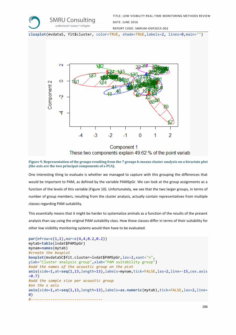
186


DATE: JUNE 2016


clusplot(mvdataS, fit$cluster, color=TRUE, shade=TRUE,labels=2, lines=0,main="")

Figure 9. Representation of the groups resulting from the 7 groups 𝐤-means cluster analysis on a bivariate plot (the axis are the two principal components of a PCA).

One interesting thing to evaluate is whether we managed to capture with this grouping the differences that

would be important to PAM, as defined by the variable PAMSpGr. We can look at the group assignments as a

function of the levels of this variable (Figure 10). Unfortunately, we see that the two larger groups, in terms of

number of group members, resulting from the cluster analysis, actually contain representatives from multiple

classes regarding PAM suitability.

This essentially means that it might be harder to systematize animals as a function of the results of the present

analysis than say using the original PAM suitability class. How these classes differ in terms of their suitability for

other low visibility monitoring systems would then have to be evaluated.

par(mfrow=c(1,1),mar=c(4,4,0.2,0.2)) mytab=table(lvdat$PAMSpGr) mynam=names(mytab) #create the boxplot boxplot(mvdataSC$fit.cluster~lvdat$PAMSpGr,las=2,xaxt="n", ylab="Cluster analysis group",xlab="PAM suitability group") #add the names of the acoustic group on the plot axis(side=1,at=seq(1,13,length=13),labels=mynam,tick=FALSE,las=2,line=-15,cex.axis=0.7) #add the sample size per acoustic group #on the x axis axis(side=1,at=seq(1,13,length=13),labels=as.numeric(mytab),tick=FALSE,las=2,line=0) #---------------------------------

187


DATE: JUNE 2016


axis(side=2,at=1:7,labels=as.numeric(table(mvdataSC$fit.cluster)),tick=FALSE,las=2,line=-2.5)

Figure 10. Cluster analysis group assignment as a function of the PAM suitability group. The numbers inside the plot represent sample sizes in each class, and the numbers below each PAM group the number of species in said group. Note that while a useful graphical representation, strictly the cluster analysis group is a qualitative variable, hence the box-plots themselves are to be interpreted with caution.

Unless the resulting patterns are strong and self-evident, it is not straightforward to interpret the output of k-

means partitioning analysis, so we also considered a hierarchical cluster approach. The key difference is one

does not need to define a priori the number of groups, but groups can be obtained by selecting a cut point on a

resulting dendogram.

We considered a Euclidean distance with Ward's linkage method (minimum variance criterion which minimizes

the total within-cluster variance of new groups). Typically different distances and linkage methods could be

attempted and the consistency of the outcome groupings assessed. This was not implemented here given the

exploratory nature of the analysis (which is also not independent of the number of available variables and their

corresponding amount of missing values).

# Ward Hierarchical Clustering # distance matrix d <- dist(mvdataS,method="euclidean") fit <- hclust(d, method="ward.D") # display dendogram par(mfrow=c(1,1),mar=c(4,4,2,1)) plot(fit,xlab="Species") # cut tree into 7 clusters groups <- cutree(fit, k=7)

188


DATE: JUNE 2016


# draw dendogram with red borders around the clusters rect.hclust(fit, k=7, border="red")

Figure 11. Dendrogram resulting from the hierarchical analysis considering the Euclidean distance and the Ward linkage method. The red boxes represent the groupings resulting from a 7 group tree cut point.

Given the large amount of species involved it is not easy to visualize the output of this analysis either (Figure

11), but a group of species names and corresponding group membership can be printed out. This is presented

as annex 2.

Instead of the typical dendrogram representation for a hierarchical analysis, Figure 12 represents the outcome

of this cluster analysis onto a bivariate plot, as before for the k-means analysis. As anticipated from the PCA

exploratory analysis the interpretation of the result is not easy.

We do note however the consistency in groupings produced by the hierarchical and partitioning approaches.

189


DATE: JUNE 2016


Figure 12. Representation of the 7 groups resulting from the hierarchical analysis on a bivariate plot (the axis are the two principal components of a PCA).

10.6.5 Conclusions

Unfortunately, the cross classification across the PAM groups and the cluster analysis leads to many of the

groups in one clustering type being distributed across multiple groups on the other grouping. Therefore the

cluster analysis does not support the existing classification according to the existing a priori PAM grouping, and

this casts doubts about whether the output of such an analysis might be usable for the other systems.

This might mean that additional variables are required to allow one to cluster species into system suitability

groups. The fact that there were many values missing which had to be imputed is also likely to have contributed

to the analysis poor performance.

One possible alternative would be to use the PAM grouping to classify the other systems against, but this might

not work if some of the groups given the acoustic suitability are not meaningful in terms of the other systems

under evaluation. A further analysis option not explored here would be to validate the PAM grouping considered

by implementing a discriminant analysis based on such grouping.

190


DATE: JUNE 2016


10.6.6 Annex

10.6.6.1 Annex 1

Below we reproduce a summary of the data set available, which provides useful information in particular it

explicitly lists the amount of missing values for each of the variables included.

summary(lvdat)

order sorder Sfam fam Carnivora :38 Caniformia : 3 Delphinoidea:45 016 :36 Cetacea :87 Cryptodira : 7 Phocoidea :34 010 :21 Lamniformes: 1 Fissipedia (marine): 1 NA :21 003 :18 Sirenia : 4 Mysticeti :15 Ziphioidea :21 001 :17 Testudines : 7 NA : 5 Chelonioidea: 7 007 : 9 Odontoceti :72 Mustelidae : 3 006 : 7 Pinnipedia :34 (Other) : 6 (Other):29 sfam gen sp Hyperoodontinae:17 Mesoplodon :14 Araus : 1 NA :16 Arctocephalus : 8 Arfor : 1 Delphininae :12 Balaenoptera : 8 Argal : 1 Lissodelphinae :10 Lagenorhynchus: 6 Argaz : 1 Phocinae :10 Stenella : 5 Arphi : 1 Arctocephalinae: 9 Balaena : 4 Arpus : 1 (Other) :63 (Other) :92 (Other):131 splat name Arctocephalus australis : 1 Amazonian manatee : 1 Arctocephalus forsteri : 1 Andrews' beaked whale : 1 Arctocephalus galapagoensis: 1 Antarctic fur seal : 1 Arctocephalus gazella : 1 Antarctic minke whale : 1 Arctocephalus philippii : 1 Arnoux's beaked whale : 1 Arctocephalus pusillus : 1 Atlantic humpback dolphin: 1 (Other) :131 (Other) :131 IUCN Critically endangered: 6 Data deficient :50 Endangered :15 Least concern :41 NA : 2 Near threatened : 8 Vulnerable :15 clizo temperate, subtropical :25 subtropical, tropical, equatorial :18 temperate, subtropical, tropical, equatorial:13 subpolar, temperate :11 tropical, equatorial :10 polar, subpolar : 8 (Other) :52 PAMSpGr BoLe_unkn BoLe_min Black Fish / Oceanic Dolphins :34 Min. :1.40 Min. : 0.510 Pinnipeds :34 1st Qu.:1.45 1st Qu.: 1.522 Beaked whales :21 Median :1.45 Median : 2.000 Quiet :13 Mean :1.78 Mean : 3.698 Porpoises / Cephalorhynchus :10 3rd Qu.:2.10 3rd Qu.: 4.575 Humpback, Right and Bowhead Whales: 7 Max. :2.50 Max. :19.000

191


DATE: JUNE 2016


(Other) :18 NA's :132 NA's :27 BoLe_Mean BoLe_Max DiDe_unkn DiDe_Min Min. : 0.660 Min. : 0.750 Min. :0.000 Min. : 0.600 1st Qu.: 1.400 1st Qu.: 2.110 1st Qu.:5.900 1st Qu.: 2.500 Median : 2.000 Median : 2.800 Median :5.900 Median : 6.000 Mean : 3.783 Mean : 5.136 Mean :5.646 Mean : 8.738 3rd Qu.: 3.033 3rd Qu.: 5.700 3rd Qu.:5.900 3rd Qu.:11.500 Max. :23.625 Max. :33.580 Max. :5.900 Max. :40.000 NA's :100 NA's :44 NA's :82 DiDe_Mean DiDe_Max DiTi_unkn DiTi_Min Min. : 3.00 Min. : 15.0 Min. :0.00000 Min. :0.001621 1st Qu.: 8.86 1st Qu.: 150.0 1st Qu.:0.01600 1st Qu.:0.023959 Median : 8.86 Median : 306.0 Median :0.02950 Median :0.046188 Mean : 68.19 Mean : 634.2 Mean :0.03996 Mean :0.083238 3rd Qu.: 25.66 3rd Qu.:1018.0 3rd Qu.:0.07080 3rd Qu.:0.106235 Max. :789.33 Max. :3200.0 Max. :0.23430 Max. :2.000000 NA's :39 NA's :4 NA's :21 NA's :21 DiTi_Mean DiTi_Max GrSi_unkn GrSi_Min Min. : 0.300 Min. : 0.480 Min. :0 Min. : 1.000 1st Qu.: 2.000 1st Qu.: 6.625 1st Qu.:0 1st Qu.: 1.000 Median : 4.000 Median : 17.500 Median :0 Median : 1.000 Mean : 9.079 Mean : 36.004 Mean :0 Mean : 2.202 3rd Qu.: 9.033 3rd Qu.: 51.800 3rd Qu.:0 3rd Qu.: 1.000 Max. :44.120 Max. :320.100 Max. :0 Max. :100.000 NA's :72 NA's :3 NA's :130 NA's :8 GrSi_Mean GrSi_Max SuTi_unkn SuTi_Min Min. : 1.310 Min. : 1.00 Min. :0 Min. :0.0030 1st Qu.: 3.292 1st Qu.: 1.25 1st Qu.:0 1st Qu.:0.0500 Median : 6.333 Median : 10.00 Median :0 Median :0.2000 Mean : 37.670 Mean : 411.71 Mean :0 Mean :0.6537 3rd Qu.: 37.208 3rd Qu.: 92.50 3rd Qu.:0 3rd Qu.:0.4400 Max. :601.700 Max. :10000.00 Max. :0 Max. :5.0000 NA's :70 NA's :7 NA's :134 NA's :112 SuTi_Mean SuTi_Max SwSp_unkn SwSp_Min Min. : 0.03 Min. : 0.01 Min. :0 Min. :0.01000 1st Qu.:11.72 1st Qu.: 1.95 1st Qu.:0 1st Qu.:0.01000 Median :11.72 Median : 9.30 Median :0 Median :0.01000 Mean :16.36 Mean : 69.79 Mean :0 Mean :0.02603 3rd Qu.:19.13 3rd Qu.: 48.80 3rd Qu.:0 3rd Qu.:0.01000 Max. :34.38 Max. :840.00 Max. :0 Max. :0.56000 NA's :12 NA's :88 NA's :136 NA's :16 SwSp_Mean SwSp_Max Min. :0.030 Min. : 0.100 1st Qu.:0.800 1st Qu.: 1.955 Median :1.317 Median : 3.340 Mean :1.203 Mean : 3.747 3rd Qu.:1.390 3rd Qu.: 5.463 Max. :3.045 Max. :11.110 NA's :67 NA's :23

192


DATE: JUNE 2016


10.6.6.3 Annex 2

Here we present the group assignments of the hierarchical analysis considering the Euclidean distance and the

Ward linkage method. Group assignment was based on 7 groups, suggested by the initial exploratory analysis

based on the K-means clustering approach.

data.frame(as.character(lvdat$name),groups)

as.character.lvdat.name. groups 1 Sea otter 1 2 Marine otter 2 3 European otter 2 4 Polar bear 2 5 South American fur seal 3 6 Subantarctic or Amsterdam Island fur seal 3 7 Guadalupe fur seal 3 8 South African & Australian or cape fur seal 3 9 Juan Fernandez fur seal 3 10 Antarctic fur seal 3 11 Galapagos fur seal 3 12 New Zealand fur seal 3 13 Northern fur seal 3 14 Steller's sea lion 3 15 Australian sea lion 3 16 South (American) sea lion 3 17 Hooker's or New Zealand sea lion 3 18 California sea lion 3 19 Galapagos sea lion 3 20 Walrus 3 21 Leopard seal 3 22 Weddell seal 3 23 Crabeater seal 3 24 Northern elephant seal 4 25 Southern elephant seal 4 26 Mediterranean monk seal 3 27 Hawaiian monk seal 3 28 Ross seal 3 29 Hooded seal 3 30 Bearded seal 3 31 Gray seal 3 32 Ribbon seal 3 33 Harp seal 3 34 Largha or spotted seal 3 35 Harbour seal 3 36 Ringed seal; synonym for Phoca hispida. 3 37 Baikal seal 3 38 Caspian seal 3 39 North Atlantic right whale 5 40 North Pacific right whale 5 41 Bowhead whale 5 42 Southern right whale 5 43 Pygmy right whale 2 44 Gray whale 5 45 Omura's whale 1 46 Fin whale 5 47 Antarctic minke whale 2

193


DATE: JUNE 2016


48 Blue whale 5 49 Common minke whale 2 50 Sei Whale 5 51 Bryde's whale 5 52 Eden's whale 5 53 Humpback whale 5 54 Franciscana 2 55 Beluga or white whale 2 56 Narwhal 4 57 Short-beaked common dolphin 6 58 Long-beaked common dolphin 6 59 Fraser's dolphin 2 60 Indo-Pacific humpback dolphin 2 61 Atlantic humpback dolphin 2 62 Clymene dolphin 2 63 Striped dolphin 2 64 Pantropical spotted dolphin 2 65 Spinner dolphin 2 66 Atlantic spotted dolphin 2 67 Indo-Pacific bottlenose dolphin 2 68 Common bottlenose dolphin 6 69 Pygmy killer whale 2 70 Long-finned pilot whale 2 71 Short-finned pilot whale 2 72 Risso's dolphin 6 73 Melon-headed whale 2 74 False killer whale 2 75 Commerson's dolphin 2 76 Chilean dolphin 2 77 Heaviside's dolphin 2 78 Hector's dolphin 2 79 Pacific white-sided dolphin 6 80 Peale's dolphin 2 81 Hourglass dolphin 2 82 Dusky dolphin 2 83 Northern right whale dolphin 2 84 Southern right whale dolphin 2 85 Atlantic white-sided dolphin 2 86 White-beaked dolphin 2 87 Irrawaddy dolphin 2 88 Australian snubfin dolphin 2 89 Killer whale 2 90 Tucuxi 2 91 Costero 2 92 Rough-toothed dolphin 2 93 Spectacled porpoise 2 94 Finless porpoise 2 95 Harbour porpoise 2 96 Vaquita 2 97 Burmeister's porpoise 2 98 Dall's porpoise 2 99 Boto 1 100 Baji 2 101 Sperm whale 4 102 Dwarf sperm whale 4 103 Pygmy sperm whale 4 104 South Asian river dolphin 1

194


DATE: JUNE 2016


105 Northern bottlenose whale 4 106 Southern bottlenose whale 4 107 Longman's beaked whale or tropical Bottlenose whale 4 108 Ginkgo-toothed beaked whale 4 109 Stejneger's beaked whale 4 110 Perrin's beaked whale 4 111 Pygmy beaked whale 4 112 True's beaked whale 4 113 Andrews' beaked whale 4 114 Spade-toothed beaked whale 4 115 Hector's beaked whale 4 116 Sowerby's beaked whale 4 117 Strap-toothed whale 4 118 Hubb's beaked whale 4 119 Blainville's beaked whale 4 120 Gray's beaked whale 4 121 Gervais' beaked whale 4 122 Tasman or Shepherd's beaked whale 4 123 Arnoux's beaked whale 4 124 Baird's beaked whale 4 125 Cuvier's beaked whale 4 126 Basking Shark 2 127 Dugong 2 128 Amazonian manatee 2 129 West Indian manatee 2 130 West African manatee 2 131 Leatherback turtle 2 132 Loggerhead sea turtle 7 133 Common green sea turtle 7 134 Hawksbill sea turtle 7 135 Olive ridley sea turtle 7 136 Kemp's Ridley sea turtle 7 137 Flatback turtle 7

195


DATE: JUNE 2016


10.8 System names addressed in the questionnaires

Table 31. Names of those companies who filled in the technical questionnaires for PAM, AAM, spectral cameras and RADAR as well as the interface questionnaire (see chapter 12.1.3 to 12.1.8). Details are given on the system(s) they addressed.

Questionnaire Company name System name/model/brand

AAM Brainlike, Inc. Brainlike Processor: An early stage version of Brainlike Processor was used for proof-of-concept purposes several years ago under contract with the U.S. Navy. Since then, Brainlike Processor (TM) has been refined for commercial use, in settings where "triage" may be performed on active sonar time series data on sonobuoys, reducing the time series data to snippets that may be transmitted over low bandwidth channels. To date, no further development has been completed because no commercial needs have yet been identified.

AAM Coda Octopus Products Ltd Echoscope

AAM Nautel C-Tech Limited CMAS-36/39 OMNI Sonar ® System

AAM Scientific Solutions, Inc SDSN (same as DOE AAM system)

AAM Scientific Solutions, Inc. HFM3

AAM Sonardyne International Ltd Sentinel

AAM Tritech International Limited Gemini 720

Other methods Brainlike, Inc. Brainlike Processor (TM).

Other methods RDE (Rheinmetall) Automatic Infrared-based Marine Mammal Mitigation System (AIMMMS)

Other methods St Andrews Instrumentation Ltd Decimus

Other methods Teledyne RESON UK Ltd SeaBat

PAM Abakai International LLC

PAM Bio-Waves Inc. custom towed array system

PAM Brainlike, Inc. Brainlike Processor (TM)

PAM Chelonia Ltd F-POD

PAM Coda Octopus Products Ltd CodaOCtopus Echoscope

PAM Columbia University Streamer based PAM

PAM Gardline Environmental GEL 2

PAM Gardline Environmental Ltd Seiche, New Leap, GEL 2 channel, Vanishing point

PAM GeoSpectrum Technologies Inc. GeoSpectrum provides a variety of products suitable for real-time PAM from individual components to end-to-end systems. These include sensors [wideband omnidirectional hydrophones up to 1 Hz - 200 kHz, high frequency vector sensing hydrophones (50 Hz to 20 kHz), 3-D particle motion sensors (1 Hz to 3 kHz), acoustic arrays 1 Hz to 200 kHz], pre-amps and signal conditioning, cabling, pressure cases, handling systems (e.g. winches), mooring systems, interface electronics, and PAM processing.

PAM MSeis Night Hawk III

PAM NAUTA ricerca e consulenza scientifica

farONE

PAM Passive Acoustic Monitoring Online Services (PAMOS)

PAM Quiet-Oceans Ocean Noise Console

PAM SANYA INSTITUTE OF DEEP-SEA SCIENCE AND ENGINEERING, CHINESE ACADEMY OF SCIENCES

PAM Seiche Seiche PAM

PAM SERCEL QuietSeaTM

196


DATE: JUNE 2016


PAM St Andrews Instrumentation Ltd Decimus

PAM Teledyne RESON UK Ltd SeaBat

PAM TNO Delphinus towed array system

PAM University Toulon ONCET

PAM Vanishing Point towed PAM streamers

RADAR Brainlike, Inc. Brainlike Processor (TM) Several years ago, Brainike completed an early-stage evaluation of gray whale detectability using with airborne Furuno RADAR. We concluded that whale blips can indeed be picked up, but that feature extraction methods would be necessary to increase detection precision (higher hit rates, lower false alarms), especially in high sea states or other settings where false blips from fishing floats, etc. might be present. Since then, Brainlike Processor has been refined to the point where developing related methods could be feasible, although sufficiently attractive commercial opportunities have not yet been identified to warrant further development.

RADAR National Oceanography Centre Kelvin Hughes RADAR, WaMoS II digitiser

RADAR RADAR Technology AS RADAR Technology Optimized Surface Detection RADAR systems

RADAR Sea-Hawk Navigation Sea-Hawk SHN X9

Spectral Camera Brainlike, Inc. Nikon D800 (36 megapixel) camera. This is a conventional, commercial RGB camera. PixMin (TM) identified marine mammals automatically from photos that were taken from 300 meters with a 50 mm lens. The cameras were mounted on the left and right side of the aircraft at an angle, covering about a swath about 1.3 KM in length. Ground Pixel resolution varied from 6 cm at Nadir to 33 cm at outboard locations. Photos were taken every 3 seconds, resulting in an overlap of about 30%. Reports describing the most recent success (for camera-based whale detection) have been uploaded to the SMRU website as part of responses to other low-visibility questionnaires.

Spectral Camera Current Scientific Corporation Night Navigator

Spectral Camera MDA Information Systems LLC

Spectral Camera Ocean Life Survey FLIR

Spectral Camera Polaris Sensor Technologies, Inc. Pyxis 640 LWIR - enhanced Thermal. See attached for further description.

Spectral Camera Rheinmetall AIMMMS

Spectral Camera Seiche Measurement Limited Camera Monitoring System (CMS)

Spectral Camera Statoil AIMMMS

Spectral Camera Telops Hyper-Cam

Spectral Camera Toyon Research Corporation

Spectral Camera Xenics Gobi / Onca

System interface Brainlike, Inc.

System interface Chelonia Ltd F-POD

System interface Coda Octopus Products Ltd Ecoscope

System interface Columbia University

System interface Current Scientific Corporation Night Navigator

System interface Gardline Environmental GEL 2

System interface Gardline Environmental Ltd Seiche, Vanishing Point, GEL 2 channel and New Leap

System interface GeoSpectrum Technologies Inc. Various: GeoSpectrum has a range of products that are suitable for low visibility real-time monitoring of marine mammals

System interface MDA Information Systems LLC MDA IS LLC System

System interface MSeis

197


DATE: JUNE 2016


System interface National Oceanography Centre Kelvin Hughes RADAR and WaMoS II digitiser

System interface Nautel C-Tech Limited CMAS-36/39 OMNI Sonar ® System

System interface Ocean Life Survey FLIR

System interface PAMOS

System interface Polaris Sensor Technologies, Inc. Pyxis® 640 LWIR

System interface Prove

System interface Quiet-Oceans Ocean Noise Console

System interface RADAR Technology AS RADAR Technology Surface Detection RADAR systems

System interface RDE (Rheinmetall) Automatic Infrared-based Marine Mammal Mitigation System (AIMMMS)

System interface Scientific Solutions, Inc. SDSN/AAM

System interface Scientific Solutions, Inc. HFM3

System interface Sea-Hawk Navigation Sea-Hawk SHN X9

System interface Seiche Seiche

System interface Seiche Measurement Limited Camera Monitoring System (CMS)

System interface SERCEL QUIETSEA

System interface St Andrews Instrumentation Ltd Decimus

System interface Teledyne RESON UK Ltd SeaBat

System interface TNO Delphinus system

System interface Toyon Research Corporation WADE and WAVE

System interface Tritech International Limited Gemini 720

System interface University Toulon ONCET

198


DATE: JUNE 2016


10.9 List of suppliers, developers and users

Table 32. List of suppliers, developers and users of systems mentioned in the questionnaire survey.

Company name Company address Key contact name Key contact phone number

Key contact email Website Developer / supplier / user

Method

Abakai International LLC

94-275 Makau St, Makaha, Hawaii, USA, 96792

Tom Fedenczuk 808-391-8595 [email protected]

Developer/user PAM

Bio-Waves Inc. Bio-Waves Inc. 364 2nd Street, Suite #3 Encinitas, CA 92024

Thomas Norris (president)

(760) 452-2575 [email protected]

http://biowaves.net/ Developer; Supplier

PAM

Aptomar AS Stiklestadveien 3 7041 Trondheim Norway

+47 40 00 34 03 [email protected] www.aptomar.com Developer Thermal

Brainlike, Inc. 1855 First Ave., Suite 103 San Diego, CA 92101 USA

Robert J. (BOB) Jannarone

619-887-1153 [email protected]

http://www.brainlike.com/

Developer; Supplier; User

Processor/ software

Chelonia Limited The Barkhouse North Cliff Mousehole TR19 6PH UK

NIck Tregenza 44 (0)1736 732462

[email protected]

Developer; Supplier

PAM

Coda Octopus Products Ltd

Anderson House 1 Breadalbane Street Edinburgh EH6 5JR, UK

Richard Adams 07799 838288 [email protected]

Developer; Supplier

AAM

Columbia University

303B Oceanography 61 Route 9W - PO Box 1000 Palisades, NY, 10964

Shima Abadi

[email protected] http://www.ldeo.columbia.edu/~shimah/

Developer PAM

Current Scientific Corporation

2933 Murray St Port Moody, BC, CANADA V3H 1X3

Aaron Ridinger 1-604-461-5555 [email protected] www.currentcorp.com Developer Thermal

Fugro Emu Ltd Trafalgar Wharf (Unit 16) Hamilton Road Portchester Portsmouth Hampshire PO6 4PX, UK

Alastair Mackay 07775 680560 [email protected]

User PAM

199


DATE: JUNE 2016




Method

Gardline Environmental

Endeavour House, Admiralty Road, Great Yarmouth, Norfolk, NR30 3NG, UK

Breanna Evans, Maja Nimak-Wood

1493845600 [email protected]

User PAM

GeoSpectrum Technologies Inc.

10 Akerley Blvd, Suite 19, Dartmouth, NS, Canada, B3B 1J4

Arnold Furlong (902) 406-4111 Ext 204

[email protected] www.geospectrum.ca Developer/user PAM

Kaon Ltd Kaon Ltd 5 Wey Court Mary Road Guildford Surrey GU1 4QU, UK

Ian Pickering 07921215335 [email protected] http://www.kaon.co.uk/products/mmad/

Developer Software

Koç Bilgi ve Savunma Teknolojileri A.S. (Koc Information & Defence Technologies Inc.)

Üniversiteler Mah. İhsan Doğramacı Blv. No:17/B ODTÜ Teknokent Ankara / TURKEY

Yavuz Atabek +902165561534 [email protected] http://www.kocsavunma.com.tr/en/Pages/default.aspx

Developer PAM

Kongsberg Maritime Subsea

PO Box 111 3191 Horten Norway

Frank Reier Knudsen

+4799214001 [email protected]

Developer; Supplier

AAM

LGL Ecological Research Associates, Inc.

4103 S. Texas Ave, Suite 211 Bryan, TX 77802, USA

Darren Ireland 406-577-2269 [email protected]

Developer High res camera

Liquid Robotics Incorporated

1529 Moffett Park Drive, USA Eric Niven +1 408 636 4266 [email protected] http://liquidr.com/ Developer; Supplier; User

Platform

MDA Information Systems LLC

Cynthia Dacre 240 833 8213

[email protected]

www.mdaus.com Developer; Supplier; User

Spectral

MSeis Limited 43A Sandford Road, Weston-super-Mare, Somerset, BS23 3EX, UK

Mark Higginbottom

+447711116070 [email protected] http://www.mseis.com/

Developer; Supplier

PAM

National Oceanography Centre

Joseph Proudman Building, 6 Brownlow street, Liverpool L35DA, UK

Paul Bell 0151 7954807 [email protected] noc.ac.uk Developers ; Users

RADAR

NAUTA ricerca e consulenza scientifica

strada della carita' 8 20135 Milano Italy

Michele Manghi +390230312139 [email protected] www.nauta-rcs.it Developer; Supplier; User

PAM

200


DATE: JUNE 2016




Method

Nautel C-Tech Limited

525 Boundary Road Cornwall, Ontario, K6H 6K8 Canada

Kirk Zwicker +1 902 823 5140 [email protected] http://nautelc-tech.com/

Developer and Supplier

AAM

NOAA Fisheries, Southwest Fisheries Science Center

8901 La Jolla Shores Drive, USA David Weller 8585465674 [email protected]

Developer; User Thermal

Ocean Life Survey NZ & UK Martin Stanley

[email protected]

www.oceanlifesurvey.com

User/Developer/Researcher

Thermal

Oregon State University

(Personal address:) 2030 SE Marine Science Dr. Newport, OR 97365, USA

Dave Mellinger +1-541-757-7953 [email protected]

http://www.bioacoustics.us/

Developer PAM

Passive Acoustic Monitoring Online Services (PAMOS)

Protasio Tagle 8-1, San Miguel Chapultepec, Miguel Hidalgo, Mexico City, 11850, Mexico

Jessica Fisher +5215538070738 [email protected] http://www.pamos.ca Developer PAM

PGS Geophysical 4 the Heights, Brooklands, Weybridge, Surrey KT13 0NY, UK

David Anderson 01932 375479 [email protected]

www.pgs.com User PAM

Polaris Sensor Technologies, Inc.

200 Westside Square, Suite 320, Huntsville, AL 35801, USA

David Chenault (256) 562-0087 ext 2436

[email protected]

www.PolarisSensor.com

Developer Thermal

Prove Systems Ltd Unit 1 Mill Court Mill Lane TAYPORT DD6 9EL Fife Scotland UK

P. Hubert 01382 552085 [email protected]

Developer; User AAM

Quest Innovations BV - Quest Group

Industrieweg 41 NL-1775 PW Middenmeer the Netherlands

Igno Breukers - Chief Commercial Officer

+31652515854 [email protected]

http://www.quest-innovations.com

Developer Spectral

Quiet-Oceans 65 place Nicolas Copernic 29280 Plouzane France

Thomas Folegot +33 982 282 123 [email protected]


PAM

Radar Technology AS

RADAR Technology AS Glasskaråsen 72, N 5106 Øvre Ervik, Bergen, Norway

Sten Wärnfeldt Tel: +46 706 386 396

[email protected], [email protected]

http://www.radar-technology.com

Developer; Supplier

RADAR

RDE (Rheinmetall) Brüggeweg 54 28309 Bremen Germany

Jens Zabel / Joerg Kleinsteinberg

+49 421 457 1674

[email protected]

Developer; Supplier

Thermal

Resource Mapping

62 Grove Street Turners Falls, MA 01376, USA

Dana Slaymaker 413 325 5574 [email protected]

http://www.resourcemappinggis.com

Developer Spectral camera

201


DATE: JUNE 2016




Method

SANYA INSTITUTE OF DEEP-SEA SCIENCE AND ENGINEERING, CHINESE ACADEMY OF SCIENCES

62 FENGHUANG ROAD, SANYA, HAINAN PROVINCE, CHINA

SONGHAI LI 8689888222393 [email protected] http://www.sidsse.cas.cn/jgsz/yjxt/shkx/brsw/

User PAM

Scientific Solutions, Inc.

99 Perimeter Road Nashua, New Hampshire, 03063 USA

Dr. Peter J. Stein 1-603-321-5042 [email protected]

Developer AAM

Sea-Hawk Navigation AS

Vaagsgaten 22 Post Box 157 Laksevaag 5847 Bergen Norway

John Soreide +47 56112311 [email protected]

Developer; Supplier

RADAR

Seiche Measurements Ltd

Bradworthy Industrial Estate Langdon Road Bradworthy Holsworthy Devon EX22 7SF United Kingdom

Phil Johnston +44 (0) 1409 404050

[email protected] http://www.seiche.com/

Developer; Supplier

PAM, Thermal

SERCEL 12 rue de la Villeneuve 29200 BREST FRANCE

LAURENT GUERINEAU

+33 2 98 05 59 50

[email protected]

http://www.sercel.com/products/Pages/QuietSea.aspx

Developer; Supplier

PAM

SMRU Consulting 1802 One MidTown 11 Hoi Shing Street Tseun Wan West Hong Kong SAR

Lindsay Porter +852 3428 3873 [email protected]

User PAM

Sonardyne Blackbushe Business Park, Yateley, Hampshire, UK

Ross Gooding 1252872288 [email protected]

www.sonardyne.com Supplier; Developer

AAM

St Andrews Instrumentation Ltd

Unit 3 Mill Court, Industrial Estate Tayport Fife DD6 9EL, UK

Richard Baggaley 01334845260 [email protected]

Developer; Supplier

PAM

Statoil ASA P.b.1004 NO-3905 Porsgrunn Norway

Jürgen Weissenberger

+47 41681659 [email protected]

User Thermal, AAM

202


DATE: JUNE 2016




Method

Teledyne RESON UK Ltd

7A Crombie Lodge Campus 2, Balgownie Drive Bridge of Don Aberdeen AB22 8GU, UK

John Fraser 01224709900 [email protected]

Developer; Supplier

PAM

Telops Quebec, Qc, Canada G2E 6J5 Vincent Farley 418-864-7808 [email protected]

Supplier Spectral

TNO, Acoustics & Sonar research group

Oude Waalsdorperweg 63 The Hague, The Netherlands

Dr. Frans-Peter A. Lam

+31 6 10553122 [email protected]

Developer; User PAM

Toyon Research Corporation

6800 Cortona Drive, Goleta, CA, USA

Kevin Sullivan 805-968-6787 x156

[email protected] www.toyon.com Developer; Supplier; User

Thermal

Tritech International Limited

Westhill Business Park Peregrine Road Westhill Aberdeenshire AB32 6JL, UK

Scott McLay 01224 744111 [email protected]

http://www.tritech.co.uk/

Supplier AAM

Ultra Electronics Sonar Systems

Waverley House Hampshire Road Weymouth, Dorset DT4 9XD England

Peter Dobbins + 44 (0)7949 836503

[email protected]

http://www.ultra-sonar.com


AAM

University of Toulon, DYNI LSIS lab

GLOTIN avenue de l'université Univ. de Toulon, BP20132-83957 La Garde CEDEX-France

Glotin +33 4 94 14 28 24

[email protected]

Developer PAM

VP Marine 8 Admiral's Hard, Steonehouse Plymouth, Devon PL1 3LR, UK

Thom Gordon 07870924513 [email protected]

Developer; Supplier

PAM

Xenics Ambachtenlaan 44 B 3001 Leuven

Georges Vejnar +33607673960 [email protected]

Developer, Supplier

Spectral

203


DATE: JUNE 2016


10.10 Questionnaires

10.10.1 Questionnaire 1: Company Questions

Company name

Company address

Key contact name

Key contact phone number

Key contact email

Your name (if different from above)

Website

Are you a developer / supplier / user?

10.10.2 Questionnaire 2: Practical Questions

System name/model/brand

1 - Brief description of system

This is a PAM/AAM/Spectral camera/RADAR/Other method system

Please link to any information about the system (e.g. website, flier, brochure) or use the upload button at the end of this questionnaire

2 - Are there any trade restrictions on the system? (e.g. export restrictions)

If yes, what are these trade restrictions?

3 - Development Stage (Proof of concept / demonstration testing / field testing / routine use (industry) / routine use (science))

4 - What components does your system include?

5 - Purchase Price for one Complete Functioning System (USD) (<$10,000 / $10-20,000 / $20-50,000 / $50-100,000 / $100,000+)

6 - Can the equipment be leased?

If yes - please provide estimated equipment lease for one week in USD

7 - How many personnel are typically needed to run equipment?

8 - What level of training is required to run equipment? (Low (days) / Moderate (weeks) / High (experts only))

9 - What platform is the system typically used on? (Vessel, buoy, AUV, UAS, plane, other)

10 - How easily can the device/system be fitted onto the platform of choice? (easy and within a few hours / with moderate effort within a day or two / only with high effort)

10A - Would you need specialists to fit it?

11 - Can the fitting be done without disturbing other platform activities?

12 - Can the system be fitted to a vessel when at sea?

204


DATE: JUNE 2016


13 - When fitted, how long does it take to set up the mitigation monitoring running?

14 - What type of installation is normally done? (permanent / temporary)

15 - Does your system require specialists for using and maintaining it?

16 - Packed for transportation, what is the system's WEIGHT (kg)?

The SIZE (in cm x cm x cm)?

17 - What software are used for monitoring?

18 - Is marine mammal detection capability real-time or near real-time (to be able to react upon animal detection for mitigation purposes)?

If not (near) real time is it possible to achieve this and are there plans to do so?

19 - Typical detection range (m) under IDEAL conditions for:

A LARGE cetacean (>10m):

Is this detection range an estimate or based on empirical data?

A MEDIUM cetacean (3-10m):


A SMALL cetacean (<3m):


A GROUP of SMALL cetacean (<3m):


A SEAL:


A TURTLE:


24 - What are the main factors affecting the detection efficiency of the system? Please specify for different situations and different species.

25 - What are the factors affecting the effectiveness of mitigation / the constraints on the use of this technology during a seismic survey?

(weather / distance from shore / vessel size / political / security / environmental / other / none)

Please describe these factors / constraints in more details if feasible.

26 - What factors can be suggested to improve the effectiveness of mitigation during seismic survey or other activities?

27 - Do you collect or are data available on marine mammal detection performance or mitigation effectiveness?

If yes - could they be made available to us (anonymized if necessary)? Please provide information on how they might be accessed.

28 - Are reports on marine mammal detection performance available? If so please provide references and/or reports (opportunity for links and uploads at the end of this questionnaire).

205


DATE: JUNE 2016


29 - Would you be interested in collaborating in an exercise to compare the effectiveness of available techniques?

10.10.3 Questionnaire 3a: PAM Questions

1 - What type of equipment and services does / could come with your system? (hydrophone streamers and deck cables / deployment winches / dry end analogue electronics / digitisation systems (sound cards etc) / computers and processing software / PAM monitoring personnel)

2 - Is the system provided as full kit and/or as individual components?

3 - Which of these additional services do you provide? (PAM MMO services / analysis and reporting / remote monitoring of PAM equipment / none)

If you are able to provide additional services please detail them here:

4 - Are PAM systems: (provided and fitted on a survey by survey basis / part of the long term equipment on the seismic vessel / other)

If other please specify:

5 - What is the general nature of the hydrophone array? (an additional standalone streamer / existing hydrophones in the seismic streamers / additional dedicated hydrophones in the seismic streamers / other)

If other please specify:

6 - How many hydrophones (or hydrophone pairs) are provided in a standard hydrophone?

7 - What is a typical equipment set provided for a project? How much redundancy is typically incorporated?

8 - What is the frequency range over which your system is sensitive (from minimum Hz to maximum Hz)?

9 - Over which frequency range is the response close to being flat (+/- 6dB)?

10 - To what extent are the hydrophones calibrated?

(known manufacture's specifications / calibration of an example Type array / calibration of each individual array)

If your hydrophones are calibrated - over what frequency range are they calibrated?

11 - What are typical sensor spacing and configurations?

12 - Does the system have any other sensors?

(depth / temperature / heading / orientation)

13 - Are hydrophones and sensors solid-moulded or enclosed in fluid-filled tubes?

14 - What is the typical tow cable length provided (m)?

15 - What is the typical length deployed (m)?

16 - How is the hydrophone typically deployed?

(by hand / by dedicated powered winch provide as part of the equipment package / by powered winch provided on vessel)

17 - Who typically deploys the equipment?

(vessel crew / PAM operator, MMO)

206


DATE: JUNE 2016


18 - On what proportion of jobs is a bespoke deployment solution provided by seismic contractor?

19 - Can hydrophone depth be adjusted? If so, how?

20 - What is the deployment depth range (m) (minimum / maximum)

21 - How are signals provided from aft deck to instrument room

(analogue / digital)

22 - Can hydrophones and programs be monitored elsewhere on the boat using ethernet or wifi? (ethernet / wifi)

How frequently is this implemented?

23 - Is analogue conditioning (e.g. topside amplifiers and filters) provided as part of equipment?

24 - Is digitisation provided as part of equipment? If so, what types and specs (bit depths, sample rates etc) of digitisers are used?

25 - Are computers provided as part of the equipment?

(PC / Mac / Desktop / Laptop / none)

26 - Is it possible to make measurements of absolute noise levels? If so, are these measurements routinely made? How are they used?

27 - How does HEAVY RAIN effect detection ranges?

(equal to ideal conditions / small reduction / moderate reduction / major reduction / no detection beyond 100m / don't know)

28 - How does HIGH SEASTATE (>4 Beaufort) effect detection range?


10.10.4 Questionnaire 3b: AAM Questions

1 - Sonar Source Level: What is the MAXIMUM (ref 1 u Pa RMS @ 1m)?

What is the TYPICAL (ref 1 u Pa RMS @ 1m)?

2 - In which frequency bands can the sonar operate?

3 - What durations, bandwidths and types of pulses can the sonar produce? (ie: 100 ms, 50 Hz hyperbolic frequency modulated, rectangular-weighted pulse)

4 - Operating depth of the sonar: What is the MINIMUM (cavitation depth)?

What is the MAXIMUM operating depth?

5 - Detection range of the sonar: What is the MINIMUM (for the shortest pulse length) range in meter?

What is the MAXIMUM (the limit of processing and display, not target specific) range in meter?

6 - What range resolutions does the sonar provide?

7 - What is the minimum transmit beam width of the sonar (measured between half power points): HORIZONTAL (azimuth)?

VERTICAL?

8 - What is the relative power level of the highest transmit side-lobe, with respect to the main lobe?

207


DATE: JUNE 2016


9 - What is the receiver dynamic range at the receive element?

10 - What is the minimum receive beam width of the sonar (horizontal beam width measure between half power points): HORIZONTAL (azimuth) (in degree)?

VERTICAL (in degree)?

11 - What is the directivity index of the receiver (in dB)?

12 - What is the highest (relative power) receiver side-lobe level?

13 - Is the sonar capable of beam steering in the vertical direction?

If yes, please describe the vertical beam-steering capability (for example, maximum/elevation angles with positive angles being down from the horizontal)

15 - Is there a sonar blind spot after a typical installation?

If yes, please describe the blind spot limitations.

16 - What is the amount of time (minutes) required to scan for targets over a 360 degree scan at all available depression angles?

17 - Does the sonar implement beam stabilization to compensate for ship motion (pitch, roll, and yaw)?

18 - Does the sonar implement own-Doppler nullification to compensate for ship motion (speed of advance)?

19 - Does the sonar support fusion of data from multiple pings?

20 - Will the sonar automatically detect and highlight potential targets?

21 - What is the minimum target speed required to detect motion with respect to the stationary bottom?

22 - Will the sonar automatically track contacts?

23 - What ability does the sonar provide to classify marine mammal contact from other potential targets such as schools of fish?



25 - How does HIGH SEASTATE (>4 Beaufort) effect detection ranges?


If you wish to link to or attach any helpful information, please do so here.

10.10.5 Questionnaire 3c: Spectral Camera Questions

1 - How many sensors does the system have?

2 - Is the location of the sensors central or distributed?

3 - Please specify the sensor type

4 - Does the system use a cryogenic cooled sensor?

If yes, please specify the cooling system

208


DATE: JUNE 2016


5 - Please specify what the minimum and maximum temperature is the system can perform in (min °C to max °C)

6 - What is the Field of View (FOV) angle (in degree): Horizontal FOV

Vertical FOV?

7 - What is the spatial resolution of the system (in degree per pixel)

8 - If infrared: Is the camera band long wave or mid wave infrared?

9 - How many images per second does the system record?

10 - How many units are necessary for a horizontal 360° field of view?

11 - Is the system forward looking?

12 - Is the system abeam looking?

13 - Is the system aft looking?

14 - Which pitch/roll stabilization type are you using?

(none / cardanic / gimbal / don't know)

15 - Which pitch/roll correction are you using?

(None / mechanical / electronic / don't know)

16 - What is pitch/roll stabilization range of your system (in +/- degree)?

17 - What is the thermal resolution (in degree Kelvin)?

18 - What is the system resolution?

19 - What are the spectral bands of the system?

20 - At what height should the system be deployed?

21 - At what platform speeds can the system operate under?

22 - What is the dynamic range of the system?

23 - How does NIGHT-TIME effect detection ranges?


24 - How does FOG effect detection ranges?






27 - How does SEA SURFACE GLARE effect detection ranges?


209


DATE: JUNE 2016



10.10.6 Questionnaire 3d: RADAR Questions

1 - Instrumented range of system (if less than 360 degrees): Please specify the MINIMUM range (in degree)

the MAXIMUM range (in degree)

2 - What is the beam width (in degree) in AZIMUTH?

in ELEVATION?

3 - What is the range resolution (and/or pulse width)?

4 - What is the transmitted power level: in PEAK level?

in AVERAGE level?

5 - What is the system noise figure?

6 - What is the azimuth scan rate?

7 - In what Polarisation(s) does the system operate (VV, HH, VH, HV, RCP, LCP, etc – list all modes.)?

8 - Does the system have target detection and tracking?

9 - Are the raw output signals and/or data accessible to allow connection to a custom RADAR processor?

10 - What electrical input power does the system need?








10.10.7 Questionnaire 3e: Other Methods Questions

1 - What is the method of your system called?

2 - How does it work?

3 - What are the key strengths of the system?

4 - What are the key weaknesses of the system?

5 - Are there particular features of the animal that effects the performance of the system?

6 - Are there particular features of the system that effects the performance of the system?

7 - What external (e.g. environmental) features effects the system performance?

210


DATE: JUNE 2016


8 - How does NIGHT-TIME effect detection ranges?








12 - How does SEA SURFACE GLARE effect detection ranges?



10.10.8 Questionnaire 4: System Interface Questions

1 - What is the name of the software used to collect data?

2 - Is the software available under public (open source) or proprietary license agreement?

3 - Does the system make data available to external software in a standard open format?

4 - If not, are there any restrictions on providing this feature?

5 - Select the appropriate data export electrical interfaces. (RS232 / RS422 / USB / IR port / ethernet / other)

6 - Can the system store a log with the details of detections, which can be accessed during and after projects (e.g., a binary or ASCII records of detections, operator annotation of the data)?

7 - Please add any additional information you would like to provide.


11 Acknowledgements We are grateful for the help and support from the advisory panel including the review of a former version of this

report. The advisory pannel included Maja Nimak-Wood (Gardline), David Hedgeland (BP), Sten Wärnsfeld

(Radar Technologies) and Roy Wyatt (Seiche Ltd.). We are also grateful to Dr. Frances C. Robertson for

contributing the earlier version of chapter 10.4., and appreciate the valuable help and support from Dr Duncan

A. Robertson on RADAR matters, and all persons taking the time to answer the questionnaires and subsequent

questions, and from the All Energy workshop participants. This work was funded by the International Association

of Oil & Gas Producers from the Joint Industry Programme on E&P Sound and Marine Life - Phase III.

211


DATE: JUNE 2016


12 Literature Cited

Abrahamsen, K. The ship as an underwater noise source. Proceedings of Meetings on Acoustics 17[1], 070058. 2014. Acoustical Society of America.

ACCOBAMS Scientific Committee. Resolution 2.16 Assessment And Impact Assessment Of Man-Made Noise. 2004. The Meeting of the Parties to the Agreement on the Conservation of Cetaceans of the Black Sea, Mediterranean Sea and contiguous Atlantic Area.

Akamatsu, T., D. Wang, K. Wang, and Y. Naito. 2005. Biosonar behaviour of free-ranging porpoises. Proceedings of the Royal Society of London B: Biological Sciences 272:797-801.

Anderson, S. J. and J. T. Morris. On the detection of marine mammals with ship-borne polarimetric microwave radar. OCEANS 2010 IEEE-Sydney , 1-6. 2010. IEEE.

Arranz, P., de Soto, N. A., Madsen, P. T., Brito, A., Bordes, F., and Johnson, M. P. 2011. Following a foraging fish-finder: Diel habitat use of Blainville’s beaked whales revealed by echolocation, PLoS One, doi: 10.1371/journal.pone.0028353.

Au, W. W. 1996. Acoustic reflectivity of a dolphin. The Journal of the Acoustical Society of America 99:3844-3848.

Au, W. W., R. A. Kastelein, K. J. Benoit-Bird, T. W. Cranford, and M. F. McKenna. 2006. Acoustic radiation from the head of echolocating harbor porpoises (Phocoena phocoena). Journal of Experimental Biology 209:2726-2733.

Au, W. W., R. A. Kastelein, T. Rippe, and N. M. Schooneman. 1999. Transmission beam pattern and echolocation signals of a harbor porpoise (Phocoena phocoena). The Journal of the Acoustical Society of America 106:3699-3705.

Bailey, H., B. Senior, D. Simmons, J. Rusin, G. Picken, and P. M. Thompson. 2010. Assessing underwater noise levels during pile-driving at an offshore windfarm and its potential effects on marine mammals. Marine pollution bulletin 60:888-897.

Baird, R. W., A. D. Ligon, and S. K. Hooker. Sub-surface and night-time behavior of humpback whales off Maui, Hawaii: A preliminary report. #40ABNC050729, 1-19. 2000.

Baldacci, A., M. Carron, and N. Portunato. 2005. Infrared detection of marine mammals. NATO Undersea Research Centre Technical Report SR-443. NATO Undersea Research Centre, New York, New York, USA.

Barkaszi, M., M. Butler, R. Compton, A. Unietis, and B. Bennet. Seismic survey mitigation measures and marine mammal observer reports. 2012. U.S. Dept. of the Interior, Bureau of Ocean Energy Management, Gulf of Mexico OCS Region, New Orleans, LA. OCS Study BOEM 2012-015. 28 p + appendices.

Barlow, J., Tyack, P. L., Johnson, M. P., Baird, R. W., Schorr, G. S., Andrews, R. D., and Aguilar de Soto, N. 2013. “Trackline and point detection probabilities for acoustic surveys of Cuvier’s and Blainville's beaked whales,” J. Acoust. Soc. Am., 134, 2486–96.

Baumgartner, M. F. and B. R. Mate. 2003. Summertime foraging ecology of North Atlantic right whales. Marine Ecology Progress Series 264.

Baumgartner, M. F., D. M. Fratantoni, T. P. Hurst, M. W. Brown, T. V. Cole, S. M. Van Parijs, and M. Johnson. 2013. Real-time reporting of baleen whale passive acoustic detections from ocean gliders. Journal of the Acoustical Society of America 134:1814-1823.

212


DATE: JUNE 2016


Baumgartner, M. F. and S. E. Mussoline. 2011. A generalized baleen whale call detection and classification system. The Journal of the Acoustical Society of America 129:2889-2902.

Beier, K. and H. Gemperlein. 2004. Simulation of infrared detection range at fog conditions for Enhanced Vision Systems in civil aviation. Aerospace Science and Technology 8:63-71.

Bernasconi M., Patel R., Nøttestad L., Knudsen F. R. and Brierley A. S. 2009. Use of active sonar for cetacean conservation and behavioral-ecology studies: a paradox? Proceedings of the Institute of Acoustics Vol. 31 Pt.1. Loughbotough, UK.

Bernasconi M., Nøttestad L., Krakstad J. O and Axelsen B. E. 2011. Dusky dolphins (Lagenorhyncus obscurus) hunting Cape horse mackerel (Trachurus trachurus capensis) in the northern Benguela Region: acoustic observation of predator-prey interactions. Marine Ecology Progress Series 429: 209-218.

Bernasconi M., Patel R and Nøttestad L. 2012. Behavioral observations of baleen whales in proximity of a modern fishing vessel. In Effects of Noise on Aquatic Life. Popper AN and Hawkins A eds Springer Science+Business Media, LLC, New York. pp: 335-338.

Bernasconi M., Patel R., Nøttestad L.. Pedersen G. and Brierley A. S. (2013a). The effect of depth on the target strength of a humpback whale (Megaptera novaengliae). Journal of the Acoustical Society of America 134(6): 4316-4322

Bernasconi M., Patel R., Nøttestad L. and Brierley A. S. (2013b) Fin whale (Balaenoptera physalus) target strength measurements. Marine Mammal Science 29(3): 371-388.

Blackwell, S. B. and C. R. Greene Jr. 2006. Sounds from an oil production island in the Beaufort Sea in summer: characteristics and contribution of vessels. The Journal of the Acoustical Society of America 119:182-196.

Blackwell, S. B., C. S. Nations, T. L. McDonald, C. R. Greene, A. M. Thode, M. Guerra, and A. Michael Macrander. 2013. Effects of airgun sounds on bowhead whale calling rates in the Alaskan Beaufort Sea. Mar Mam Sci 29:E342-E365.

Blackwell, S. B., C. S. Nations, T. L. McDonald, A. M. Thode, D. Mathias, K. H. Kim, C. R. Greene Jr, and A. M. Macrander. 2015. Effects of Airgun Sounds on Bowhead Whale Calling Rates: Evidence for Two Behavioral Thresholds. PLoS One 10:e0125720.

Boebel, O. Exploring the Thermal Limits of IR-Based Automatic Whale Detection (ETAW). 2013. DTIC Document.

BOEM, BSEE, and OCS. Implementation of Seismic Suryey Mitigatton Measures and Protected Species Observer Program. JOINT NTL No. 2012-G02. 2012. United States Department Of The Interior Bureau Of Ocean Energy Management, Bureau Of Safety And Environmental Enforcement And Gulf Of Mexico Outer Continental Shelf (OCS) Region.

Briggs, J. N. 2004. Target detection by marine radar. 16 ed. IET.

Burdic, W. S. 1991. Underwater acoustic system analysis. Prentice Hall.

Calambokidis, J., G. S. Schorr, G. H. Steiger, J. Francis, M. Bakhtiari, G. Marshall, E. M. Oleson, D. Gendron, and K. Robertson. 2007. Insights into the underwater diving, feeding, and calling behavior of blue whales from a suction-cup-attached video-imaging tag (CRITTERCAM). Marine Technology Society Journal 41:19-29.

Calupca, T. A., K. M. Fristrup, and C. W. Clark. 2000. A compact digital recording system for autonomous bioacoustic monitoring. The Journal of the Acoustical Society of America 108:2582.

213


DATE: JUNE 2016


Chapman, D. M. 2001. What are we inverting for? Pages 1-14 in Inverse problems in underwater acoustics.Springer.

Churnside, J., L. Ostrovsky, and T. Veenstra. 2009. Thermal footprints of whales. Oceanography 22:206.

Committee on Characterizing Biologically Significant Marine Mammal Behavior, Ocean Studies Board, Division on Earth and Life Studies, and National Research Council. 2005. Marine mammal populations and ocean noise - determining when noise causes biologically significant effects. The National Academies Press, Washington, DC.

Compton, R., L. Goodwin, R. Handy, and V. Abbott. 2008. A critical examination of worldwide guidelines for minimising the disturbance to marine mammals during seismic surveys. Marine Policy 32:255-262.

Cox, T. M., T. J. Ragen, A. J. Read, E. Vos, R. W. Baird, K. Balcomb, J. Barlow, J. Caldwell, T. Cranford, and L. Crum. Understanding the impacts of anthropogenic sound on beaked whales. 2006. DTIC Document.

Crum, L. A., M. R. Bailey, J. Guan, P. R. Hilmo, S. G. Kargl, T. J. Matula, and O. A. Sapozhnikov. 2005. Monitoring bubble growth in supersaturated blood and tissue ex vivo and the relevance to marine mammal bioeffects. Acoustics Research Letters Online 6:214-220.

Current Corporation. Night Navigator 3. 2011.

Cuyler, L. C., R. Wiulsrod, and N. A. Oritsland. 1992. Thermal infrared radiation from free living whales. Mar Mam Sci 8:120-134.

D'Spain, G. L., A. N. G. E. D'Amico, and D. M. Fromm. 2006. Properties of the underwater sound fields during some well documented beaked whale mass stranding events. Journal of Cetacean Research and Management 7:223-238.

DECC. 2011. Review and Assessment of Underwater Sound Produced from Oil and Gas Sound Activities and Potential Reporting Requirements under the Marine Strategy Framework Directive. Genesis Ref: J71656. Document No. J71656-Final Report –G2. Date: July 2011.

Department of the Environment Heritage and Local Government. Code of Practice for the Protection of Marine Mammals during Acoustic Seafloor Surveys in Irish Waters. 2007.

Department of the Environment Water Heritage and the Arts . Australian Government EPBC Act Policy Statement 2.1 - Interaction between offshore seismic exploration and whales . 2008.

DeProspo, DF., J. Mobley, W. Hom, and M. Carron. Radar-based detection, tracking and speciation of marine mammals from ships. 2005. DTIC Document.

DFO. Statement of Canadian Practice with respect to the Mitigation of Seismic Sound in the Marine Environment. 2013.

DFO. Review of mitigation and monitoring measures for seismic survey activities in and near the habitat of cetacean species at risk. Sci. Rep. 2015/005. 2015. DFO Can. Sci. Advis. Sec.

Di Iorio, L. and C. W. Clark. 2010. Exposure to seismic survey alters blue whale acoustic communication. Biology letters 6:51-54.

di Sciara, G. N. and J. Gordon. 1997. Bioacoustics: a tool for the conservation of cetaceans in the Mediterranean Sea. Marine & Freshwater Behaviour & Phy 30:125-146.

214


DATE: JUNE 2016


Dolman, S. and M. Simmonds. 2005. Un updated note on the vulnerability of cetaceans to Acoustic disturbance. IWC Scientific Committee SC/52 E 22.

Donovan, C. R., C. Harris, J. Harwood, and L. Milazzo. A simulation-based method for quantifying and mitigating the effects of anthropogenic sound on marine mammals. Proceedings of Meetings on Acoustics 17[1], 070043. 2014. Acoustical Society of America.

Douglas, L. A., S. M. Dawson, and N. Jaquet. 2005. Click rates and silences of sperm whales at Kaikoura, New Zealand. The Journal of the Acoustical Society of America 118:523-529.

Dunn, J. L. 1969. Airborne measurements of the acoustic characteristics of a sperm whale. The Journal of the Acoustical Society of America 46:1052-1054.

Erbe, C. 2002. Underwater noise of whale‐watching boats and potential effects on killer whales (Orcinus orca), based on an acoustic impact model. Marine Mammal Science. 18:394-418.

Fahlman, A., P. L. Tyack, P. J. Miller, and P. H. Kvadsheim. 2014. How man-made interference might cause gas bubble emboli in deep diving whales. Frontiers in physiology 5.

Fais, A. 2014. Acoustic behaviour of sperm whales (Physeter macrocephalus): applications in ecology and population studies. PhD Department of Animal Biology La Laguna, Tenerife, Spain, La Laguna.

Fais, A., T. Lewis, D. Zitterbart, O. Alvarez, A. Tejedor, and N. Aguilar Soto. 2015. Abundance and distribution of sperm whales in the Canary Islands: are ship-strikes sustainable? PLoS One Submitted.

Fernandez, A., J. F. Edwards, F. Rodriguez, A. E. De Los Monteros, P. Herraez, P. Castro, J. R. Jaber, V. Martin, and M. Arbelo. 2005. Gas and fat embolic syndrome involving a mass stranding of beaked whales (Family Ziphiidae) exposed to anthropogenic sonar signals. Veterinary Pathology Online 42:446-457.

Finneran, J. J. and A. K. Jenkins. Criteria and thresholds for US Navy acoustic and explosive effects analysis. 2012. DTIC Document.

Fretwell, P. T., M. A. LaRue, P. Morin, G. L. Kooyman, B. Wienecke, N. Ratcliffe, A. J. Fox, A. H. Fleming, C. Porter, and P. N. Trathan. 2012. An emperor penguin population estimate: the first global, synoptic survey of a species from space. PLoS ONE 7:e33751.

Fretwell, P. T., I. J. Staniland, and J. Forcada. 2014. Whales from Space: Counting Southern Right Whales by Satellite. PLoS ONE 9:e88655.

Gentry, R. Report of the workshop on acoustic resonance as a source of tissue trauma in cetaceans. 24-25 April, NMFS, Silver Spring, MD. 19 p. 2002.

Geoffroy, M., S. Rousseau, and C. Pyc. 2011 Beaufort Sea Active Acoustics Survey for Marine Mammal and Pelagic Fish Detection. 2012.

Geoffroy,M., S Rousseau, FR Knudsen, L Fortier, 2015. Target strengths and echotraces of whales and seals in the Canadian Beaufort Sea, ICES Journal of Marine Science, Volume 73, Issue 2, Pp. 451-463

Gillespie, D., M. Caillat, J. Gordon, and P. White. 2013. Automatic detection and classification of odontocete whistles. The Journal of the Acoustical Society of America 134:2427-2437.

Gillespie, D., C. Dunn, J. Gordon, D. Claridge, C. Embling, and I. Boyd. 2009. Field recordings of Gervais beaked whales Mesoplodon europaeus from the Bahamas. The Journal of the Acoustical Society of America 125:3428-3433.

215


DATE: JUNE 2016


Gillespie, D., J. Gordon, M. Caillat, D. Claridge, D. Moretti, and I. Boyd. 2008. Detection of beaked whales using near surface towed hydrophones: prospects for survey and mitigation. The Journal of the Acoustical Society of America 123:3774.

Gilroy, L. E., D. P. Brennan, and R. Byers. Predicting Target echo strength of marine mammals. The sixteenth international congress on sound and vibration, Krakow, Poland 5-9 July 2009. 2009.

Goodson, A. D. and C. R. Sturtivant. 1996. Sonar characteristics of the harbour porpoise (Phocoena phocoena): source levels and spectrum. ICES Journal of Marine Science: Journal du Conseil 53:465-472.

Gordon, J., Gillespie, D., Chappell, O., Lewis, T., Swift, R. and Belford, R.A. 2000a, May. The Role of Acoustic Monitoring in Minimising the Impact of Seismic Aquisition on Cetaceans. In 62nd EAGE Conference & Exhibition.

Gordon, J. C. D., Matthews, J. N., Panigada, S., Gannier, A., Borsani, J. F., & Di Sciara, G. N. 2000b. Distribution and relative abundance of striped dolphins, and distribution of sperm whales in the Ligurian Sea cetacean sanctuary: results from a collaboration using acoustic monitoring techniques. Journal of Cetacean Research and Management, 2(1), 27-36.

Gordon, J., D. Gillespie, J. Potter, A. Frantzis, M. P. Simmonds, R. Swift, and D. Thompson. 2003. A review of the effects of seismic surveys on marine mammals. Marine Technology Society Journal 37:16-34.

Götz, T., G. Hastie, L.T. Hatch, O. Raustein, B. Southall, M. Tasker, and F. Thomsen. 2009. Overview of the impacts of anthropogenic underwater sound in the marine environment. OSPAR Biodiversity Series. 441.

Graber, J., J. Thomson, B. Polagye, and A. Jessup. Remote sensing and modeling of ecosystems for sustainability VIII. Remote sensing and modeling of ecosystems for sustainability. 8156. 2011.

Greene Jr, C. R., M. W. McLennan, R. G. Norman, T. L. McDonald, R. S. Jakubczak, and W. J. Richardson. 2004. Directional frequency and recording (DIFAR) sensors in seafloor recorders to locate calling bowhead whales during their fall migration. The Journal of the Acoustical Society of America 116:799-813.

Greene, C. R. and S. C. Chase. 1987. Infared Detection of Whale Spouts: A Report on a Feasibility Study, 2 January 1987. Greeneridge Sciences.

Grimm, V. and S. F. Railsback. 2005. Individual-based modeling and ecology Princeton University Press. Princeton, New Jersey, USA.

Groenaas, H., S. A. Frivik, A. Melba, and M. Svendsen. A novel marine mammal monitoring system using the seismic streamer spread. SEG Conference. 2011.

Hastie, G. Tracking Marine Mammals Around Marine Renewable Energy Devices Using Active Sonar. SMRU Ltd report URN:12D/328 to the Department of Energy and Climate Change. 2012.

Hastie, G. D., C. Donovan, T. Goetz, and V. M. Janik. 2014. Behavioral responses by grey seals (Halichoerus grypus) to high frequency sonar. Marine Pollution Bulletin 79:205-210.

Hedgeland, D. A., and B. Wayne. Marine mammal mitigation and seismic operations. PESGB, PETEX 04 Conference and Technical Exhibition. 2004.

Herschel, A., S. Stephenson, C. Sparling, C. Sams, and J. Monnington. ORJIP Project 4, Phase 1: Use of deterrent devices and improvements to standard mitigation during piling. 2013. Report submitted to the Offshore Renewables Joint Industry Programme.

216


DATE: JUNE 2016


Holt, M. M., D. P. Noren, V. Veirs, C. K. Emmons, and S. Veirs. 2009. Speaking up: Killer whales (Orcinus orca) increase their call amplitude in response to vessel noise. The Journal of the Acoustical Society of America 125:27-32.

Hooker, S. K., R. W. Baird, and A. Fahlman. 2009. Could beaked whales get the bends?: Effect of diving behaviour and physiology on modelled gas exchange for three species: Ziphius cavirostris, Mesoplodon densirostris and Hyperoodon ampullatus. Respiratory physiology & neurobiology 167:235-246.

IAGC. Recommended Mitigation Measures For Cetaceans during Geophysical Operations . 2011. International Association of Geophysical Contractors.

IBAMA and MMA. Guidance to Monitoring the Marine Biota in Activities of Seismic Data Acquisition. 2005.

Ireland, D. Automated Detection of Large Cetaceans in Aerial Digital Imagery. Abstract to the conference of the Society of Marine Mammalogy, San Francisco, USA. 2015.

ISO/DIS 18405:2014(E). Underwater acoustics – Terminology. International Organization for Standardization, Geneva. 2014.

Jackson, D. R. 1994. APL-UW high-frequency ocean environmental acoustic models handbook. Applied Physics Laboratory, University of Washington, Technical Report 9407.

Jackson, D. and M. Richardson. 2007. High-frequency seafloor acoustics. Springer Science & Business Media.

Jaffe, J. S., Simonet, F., Roberts, P.L.D., and Bowles, A. E. 2007. Measurement of the acoustic reflectivity of sirenia (Florida manatees) at 171 kHz. J. Acoust. Soc. Am. 121:158–165.

Jensen, F. 1994. Computational ocean acoustics. Springer Science & Business Media.

Jepson, P. D., M. Arbelo, R. Deaville, I. A. P. Patterson, P. Castro, J. R. Baker, E. Degollada, H. M. Ross, P. Herráez, and A. M. Pocknell. 2003. Gas-bubble lesions in stranded cetaceans. Nature 425:575-576.

JNCC. Guidelines for minimising acoustic disturbance to marine mammals from seismic surveys. 1998.

JNCC. JNCC guidelines for minimising the risk of injury and disturbance to marine mammals from seismic surveys. 2010a.

JNCC. JNCC guidelines for minimising the risk of injury to marine mammals from using explosives. 2010b.

JNCC. Statutory nature conservation agency protocol for minimising the risk of injury to marine mammals from piling noise. 2010c.

Johnson, M., P. T. Madsen, W. M. Zimmer, N. A. De Soto, and P. L. Tyack. 2004. Beaked whales echolocate on prey. Proceedings of the Royal Society of London B: Biological Sciences 271:S383-S386.

Kalikhman, I. L. and K. I. Yudanov. 2006. Acoustic fish reconnaissance. CRC Press.

Kay Steven, M. Fundamentals of statistical signal processing, volume I: Estimation theory. 1993. Englewood Cliffs: Prentice Hall PTR.

Keenan, G., C. Sparling, H. Williams, and F. Fortune. 2011. SeaGen environmental monitoring programme final report. Royal Haskoning: Edinburgh, UK, January.

Ketten, D. R. 1995. Estimates of blast injury and acoustic trauma zones for marine mammals from underwater explosions. Sensory systems of aquatic mammals391-407.

217


DATE: JUNE 2016


Klinck, H., D. K. Mellinger, K. Klinck, N. M. Bogue, J. C. Luby, W. A. Jump, G. B. Shilling, T. Litchendorf, A. S. Wood, G. S. Schorr, and R. W. Baird. 2012. Near-Real-Time Acoustic Monitoring of Beaked Whales and Other Cetaceans Using a Seaglider (TM). PLoS ONE 7.

Knudsen, F. R., O. B. Gammelsætter, P. H. Kvadsheim, and L. Nøttestad. Evaluation of fisheries sonars for whale detection in relation to seismic survey operations. 36. 2007. International Association of Oil and Gas Producers (OGP).

Knudsen, F. R., O. B. Gammelsætter, P. H. Kvadsheim, and L. Nøttestad. 2008. Evaluation of fisheries sonars for whale detection in relation to seismic survey operations. Bioacoustics 17:326-328.

Koski, W. R., P. Abgrall, and S. B. Yazvenko. 2009. A Review and inventory of unmanned aerial systems for detection and monitoring of key biological resources and physical parameters affecting marine life during offshore exploration and production activities. IWC paper SC/61 E 9.

Küsel, E.T., D.K. Mellinger, L. Thomas, T.A. Marques, D.J. Moretti, and J. Ward. 2011. Cetacean population density from single fixed sensors using passive acoustics. Journal of the Acoustical Society of America 129: 3610-3622.

Kvadsheim, P., Benders, F., Miller, P., Doksæter, L., Knudsen, F., Tyack, P., Nordlund, N., Lam, F.-P., Samarra, F., Kleivane, L., and Godø, O. R. 2007. Herring (sild), Killer Whales (spekkhogger) and Sonar – the 3S-2006 Cruise Report with Preliminary Results. FFI-rapport 2007/01189, Forsvarets forskningsinstitutt/Norwegian Defence Research Establishment (FFI), Horten, Norway.

Kvadsheim, P. H., P. J. Miller, P. L. Tyack, L. D. Sivle, F. P. Lam, and A. Fahlman. 2012. Estimated tissue and blood N2 levels and risk of decompression sickness in deep-, intermediate-, and shallow-diving toothed whales during exposure to naval sonar. Frontiers in physiology 3.

Kyhn, L., J. Tougaard, K. Johansen, D. Boertmann, and A. Mosbech. Guidelines to environmental mitigation assessment of seismic activities in Greenland waters. 2011. Danish Center for Environment and Energy.

LaRue, M. A., J. J. Rotella, R. A. Garrott, D. B. Siniff, D. G. Ainley, G. E. Stauffer, C. C. Porter, and P. J. Morin. 2011. Satellite imagery can be used to detect variation in abundance of Weddell seals (Leptonychotes weddellii) in Erebus Bay, Antarctica. Polar Biology 34:1727-1737.

Leaper, R. and J. Gordon. Marine Mammal Acoustic and Visual Surveys - Analysis of Neart Na Gaoithe data. 2012. Appendix 13.5 Neart Na Gaoithe Environmental Statement. Mainstream Renewables. 20pp.

Leaper, R., D. Gillespie, J. Gordon, and J. Matthews. Abundance assessment of sperm whales. 2003. Paper SC/55/O13 presented to the IWC Scientific Committee, Berlin.

Leong, H. and A. Ponsford. The effects of sea clutter on the performance of HF surface wave radar in ship detection. Radar Conference, 2008.RADAR'08.IEEE , 1-6. 2008. IEEE.

Lerczak, J. A. and R. C. Hobbs. 1998. Calculating Sighting Distances From Angular Readings During Shipboard, Aerial, And Shore Based Marine Mammal Surveys. Mar Mam Sci 14:590-598.

Levenson, C. 1974. Source level and bistatic target strength of the sperm whale (Physeter catadon) measured from an oceanographic aircraft. J. Acoust. Soc. Am. 55:1100–1103.

Lewis, T., D. Gillespie, J. Gordon, and O. Chappell. Acoustic Cetacean Monitoring 1996 to 1999: Towards the Development of an Automated System Summary Report. A report to Shell UK Ltd. Contract C10563. 2000. Birmingham Research And Development Ltd.

218


DATE: JUNE 2016


Linnenschmidt, M., L. N. Kloepper, M. Wahlberg, and P. E. Nachtigall. 2012. Stereotypical rapid source level regulation in the harbour porpoise biosonar. Naturwissenschaften 99:767-771.

Lis, A. and D. Iwanowska. Marine Mammal Observation. 2013.

Love, R. H. 1973. Target strengths of humpback whales Megaptera novaeangliae. The Journal of the Acoustical Society of America 54:1312-1315.

Lucifredi, I. and P. J. Stein. Integrated Marine Mammal Monitoring and Protection System (IMAPS): Gray Whale Target Strength Measurements and the Analysis of the Back-Scattered Response. OCEANS 2006 , 1-6. 2006. IEEE.

Lucifredi, I., and Stein, P. J. 2007. Gray whale target strength measurements and the analysis of the backscattered response. J. Acoust. Soc. Am. 121:1383–1391.

Lucke, K., P. A. Lepper, M. A. Blanchet, and U. Siebert. 2008. Testing the acoustic tolerance of harbour porpoise hearing for impulsive sounds. Bioacoustics 17:329-331.

Madsen, P., M. Wahlberg, and B. Møhl. 2002. Male sperm whale (Physeter macrocephalus) acoustics in a high-latitude habitat: implications for echolocation and communication. Behavioral Ecology and Sociobiology 53:31-41.

Madsen, P. T., de Soto, N. A., Arranz, P., and Johnson, M. 2013. Echolocation in Blainville’s beaked whales (Mesoplodon densirostris). J. Comp. Physiol. A Neuroethol. Sensory, Neural, Behav. Physiol., 199, 451–469

Maire, F. D., L. Mejias, A. Hodgson, and G. Duclos. Detection of dugongs from unmanned aerial vehicles. Intelligent Robots and Systems (IROS), 2013 IEEE/RSJ International Conference on , 2750-2756. 2013. IEEE.

Maranda, B., L. Gilroy, J. Theriault, and E. MacNeil. Survey of Active Acoustic Monitoring (AAM) Technologies Volume III: Active Sonar Performance Factors. 2010.

Marques, T. A., L. Thomas, S. W. Martin, D. K. Mellinger, J. A. Ward, D. H. Moretti, D. Harris, and P. L. Tyack. 2013. Estimating animal population density using passive acoustics. Biological Reviews 88:287-309.

Marques, T. A., L. Thomas, J. Ward, N. DiMarzio, and P. L. Tyack. 2009. Estimating cetacean population density using fixed passive acoustic sensors: An example with Blainville's beaked whales. The Journal of the Acoustical Society of America 125:1982-1994.

Martin, N., K. St John, and G. Gill. Review of Sound and Marine Life Guidelines for Marine Seismic Operations. SPE 168412-MS. 2014. This paper was prepared for presentation at the 2014 SPE International Conference on Health, Safety, and Environment in Oil and Gas Exploration and Production held in Long Beach, California, 17-19 March 2014.

Martin, S. W., T. A. Marques, L. Thomas, R. P. Morrissey, S. Jarvis, N. DiMarzio, D. Moretti, and D. K. Mellinger. 2013. Estimating minke whale (Balaenoptera acutorostrata) boing sound density using passive acoustic sensors. Mar Mam Sci 29:142-158.

Matthews, J. N., S. Brown, D. Gillespie, M. Johnson, R. McLanaghan, A. Moscrop, D. Nowacek, R. Leaper, T. Lewis, and P. Tyack. 2001. Vocalisation rates of the North Atlantic right whale (Eubalaena glacialis). Journal of Cetacean Research and Management 3:271-282.

McDaniel, S. T. 1993. Sea surface reverberation: A review. The Journal of the Acoustical Society of America 94:1905-1922.

219


DATE: JUNE 2016


McDonald, M. A. 2004. DIFAR hydrophone usage in whale research. Canadian Acoustics 32:155-160.

McHugh, R., D. Mclaren, and S. Hayes. Hydroacoustic monitoring of piling operations in the North Sea. Proceedings of the 1st International Conference on Underwater Acoustic Measurements: Technologies and Results . 2005.

McKeogh, E., A. Borawska, and D. Craig. Final report: Marine mammal observations, passive acoustic monitoring detections during 2D long offset seismic survey, offshore Ireland. E0233. 2014. For BGP. By Geoguide Consultants Ltd. 291 Reading Road, Henley-on-Thames, Oxfordshire, RG9 1EL, UK. 39 p + appendices.

McMahon, C. R., H. Howe, J. van den Hoff, R. Alderman, H. Brolsma, and M. A. Hindell. 2014. Satellites, the All-Seeing Eyes in the Sky: Counting Elephant Seals from Space. PLoS ONE 9:e92613.

Mejias, L., G. Duclos, A. Hodgson, and F. D. Maire. 2013. Automated marine mammal detection from aerial imagery. Proceedings of OCEANS'13 IEEE/MTS.

Mellen, R. H., P. M. Scheifele, and D. G. Browning. Global model for sound absorption in sea water. 1987. DTIC Document.

Mellinger, D. K., K. M. Stafford, S. Moore, R. P. Dziak, and H. Matsumoto. 2007. Fixed passive acoustic observation methods for cetaceans. Oceanography 20:36.

Miller, B. S., J. Barlow, S. Calderan, K. Collins, R. Leaper, N. Kelly, D. Peel, P. Olson, P. Ensor, and M. C. Double. 2013. Long-range acoustic tracking of Antarctic blue whales. Rep Submitt to Sci Comm Int Whal Comm SC/65a/SH11-17.

Miller, J. H. and D. C. Potter. Active high frequency phased-array sonar for whale shipstrike avoidance: Target strength measurements. OCEANS, 2001.MTS/IEEE Conference and Exhibition 4, 2104-2107. 2001. IEEE.

Miller, P. J., M. P. Johnson, and P. L. Tyack. 2004. Sperm whale behaviour indicates the use of echolocation click buzzes 'creaks' in prey capture. Proceedings of the Royal Society of London B: Biological Sciences 271:2239-2247.

Mohl, B. and S. Andersen. 1973. Echolocation: high frequency component in the click of the Harbour Porpoise (Phocoena ph. L.). The Journal of the Acoustical Society of America 54:1368-1372.

Mohl, B., M. Wahlberg, P. T. Madsen, A. Heerfordt, and A. Lund. 2003. The monopulsed nature of sperm whale clicks. The Journal of the Acoustical Society of America 114:1143-1154.

Mollett, A., C. Schofield, I. Miller, J. Harwood, C. Harris, and C. Donovan. Environmental Risk Management Capability: Advice on Minimising the Impact of Both Sonar and Seismic Offshore Operations on Marine Mammals. Offshore Europe . 2009. Society of Petroleum Engineers.

Nedwell, J. and D. Howell. 2004. A review of offshore windfarm related underwater noise sources. Cowrie Rep 544:1-57.

New Zealand Department of Conservation. 2012 Code of Conduct for Minimising Acoustic Disturbance to Marine Mammals from Seismic Survey Operations REFERENCE DOCUMENT. 2012. Publishing Team, Department of Conservation .

Nielsen, R. O. 1991. Sonar signal processing. Artech House, Inc..

Norris, T., S. Martin, L. Thomas, T. Yack, J. N. Oswald, E. M. Nosal, and V. Janik. 2012. Acoustic Ecology and Behavior of Minke Whales in the Hawaiian and Marianas Islands: Localization, Abundance Estimation,

220


DATE: JUNE 2016


and Characterization of Minke Whale ‘Boings’. Pages 149-153 in The Effects of Noise on Aquatic Life.Springer.

OGP. 2011. An overview of marine seismic operations. Report 448:2011.

Oleson, E. M., J. Calambokidis, W. C. Burgess, M. A. McDonald, C. A. LeDuc, and J. A. Hildebrand. Behavioral context of call production by eastern North Pacific blue whales. 2007. DTIC Document.

OSPAR Commission. 2009. Overview of the impacts of anthropogenic underwater sound in the marine environment. Report 441:2009.

Oswald, J. N., S. Rankin, J. Barlow, and M. O. Lammers. 2007. A tool for real-time acoustic species identification of delphinid whistles. The Journal of the Acoustical Society of America 122:587-595.

Parks, S. E., A. Searby, A. Celerier, M. P. Johnson, D. P. Nowacek, and P. L. Tyack. 2011. Sound production behavior of individual North Atlantic right whales: implications for passive acoustic monitoring. Endanger Species Res 15:63-76.

Parks, S. E., C. W. Clark, and P. L. Tyack. 2007. Short-and long-term changes in right whale calling behavior: the potential effects of noise on acoustic communication. The Journal of the Acoustical Society of America 122:3725-3731.

Parsons, E. C. M., S. J. Dolman, M. Jasny, N. A. Rose, M. P. Simmonds, and A. J. Wright. 2009. A critique of the UKs JNCC seismic survey guidelines for minimising acoustic disturbance to marine mammals: Best practise? Marine pollution bulletin 58:643-651.

Parvin, S., E. Harland, and J. Nedwell. The Target Strength of marine mammals, and estimated performance of Active Acoustic Monitoring systems. 2007.

Pecknold, S. P., W. M. Renaud, D. R. McGaughey, J. Theriault, and R. F. Marsden. 2009. Improved active sonar performance using costas waveforms. IEEE Journal of Ocean Engineering 34:559-574.

Perryman, W. L., M. A. Donahue, J. L. Laake, and T. E. Martin. 1999. Diel Variation In Migration Rates Of Eastern Pacific Gray Whales Measured With Thermal Imaging Sensors. Mar Mam Sci 15:426-445.

Pirotta, E., K. L. Brookes, I. M. Graham, and P. M. Thompson. 2014. Variation in harbour porpoise activity in response to seismic survey noise. Biology letters 10:20131090.

Platonov, N. G., I. N. Mordvintsev, and V. V. Rozhnov. 2013. The possibility of using high resolution satellite images for detection of marine mammals. Biology Bulletin 40:197-205.

Podobna, Y., J. Schoonmaker, C. Boucher, and D. Oakley. Optical detection of marine mammals. SPIE Defense, Security, and Sensing , 73170J. 2009. International Society for Optics and Photonics.

Potter, J. R., M. Thillet, C. Douglas, M. Chitre, Z. Doborzynski, and P. J. Seekings. 2007. Visual and passive acoustic marine mammal observations and high-frequency seismic source characteristics recorded during a seismic survey. Oceanic Engineering, IEEE Journal of 32:469-483.

Pyć CD, M Geoffroy, FR Knudsen. 2016. An evaluation of active acoustic methods for detection of marine mammals in the Canadian Beaufort Sea, Marine Mammal Science.

Rankin, S. and J. Barlow. 2005. Source of the North Pacific ‘boing’ sound attributed to minke whales. The Journal of the Acoustical Society of America 118:3346-3351.

221


DATE: JUNE 2016


Rankin, S., T. F. Norris, M. A. Smultea, C. Oedekoven, A. M. Zoidis, E. Silva, and J. Rivers. 2007. A visual sighting and acoustic detections of minke whales, Balaenoptera acutorostrata (Cetacea: Balaenopteridae), in nearshore Hawaiian waters. Pacific Science 61:395-398.

Rauh, N. MMO and PAM report. Marine mammal observations and passive acoustic detections during 2D long offset marine seismic survey, Ireland. M0148. 2013. For BGP. By GeoGuide, UK. 48 p + appendices.

Rendell, L. E. and J. C. D. Gordon. 1999. Vocal response of long-finned pilot whales (Globicephala melas) to military sonar in the Ligurian Sea. Mar Mam Sci 15:198-204.

Richardson, W. J., C. R. Greene Jr, C. I. Malme, and D. H. Thomson. 1995. Marine Mammals and Noise (Academic, New York).

Ridgeway, S. H., and Howard, R. 1979. Dolphin lung collapse and intramuscular circulation during free dive. Science 206:1182–1183.

RPS. Environmental Observation Report Shell Canada Ltd Shelburne Basin 3D Seismic Survey 18th May - 31st August 2013. 2013.

RPS Energy Canada. Wildlife Observation Report BP Tangier 3D WATS Seismic Survey Halifax, Nova Scotia 17 May to 14 September 2014. 2014.

Samaran, F., C. Guinet, O. Adam, J. F. Motsch, and Y. Cansi. 2010. Source level estimation of two blue whale subspecies in southwestern Indian Ocean. The Journal of the Acoustical Society of America 127:3800-3808.

Santhaseelan, V., S. Arigela, and V. K. Asari. 2012. Neural Network Based Methodology for Automatic Detection of Whale Blows in Infrared Video. Pages 230-240 in Advances in Visual Computing.Springer.

Sarangapani S., Miller J. H., Potty G. R., Reeder D. B., Stanton T. K., Chu D. 2005. Measurements and modeling of the target strength of divers Oceans 2005 - Europe, pp 952-956 Vol. 952

Schoonmaker, J., T. Wells, G. Gilbert, Y. Podobna, I. Petrosyuk, and J. Dirbas. Spectral detection and monitoring of marine mammals. SPIE Defense and Security Symposium , 694606. 2008. International Society for Optics and Photonics.

Schreer, J. F. and K. M. Kovacs. 1997. Allometry of diving capacity in air-breathing vertebrates. Canadian Journal of Zoology 75:339-358.

Selivanovsky D. A., Ezersky A. B. (1996) Sound Scattering by Hydrodynamic Wakes of Sea Animals. ICES Journal of Marine Science 53: 377-381

Sheldon-Robert, M. K., S. P. Beeren, and F. P. A. Lam. 2008. The Delphinus array for passive marine mammal detection. Maritime Studies 12.

Silber, G., S. Betteridge, and D. Cottingham. Report of a Workshop to Identify and Assess Technologies to Reduce Ship Strikes of Large Whales. Providence, Rhode Island 8-10 July 2008. 2009. NOAA Technical Memorandum NMFS-OPR-42.

Simmonds, J. and D. N. MacLennan. 2008. Fisheries acoustics: theory and practice. John Wiley & Sons.

Simrad AS. Evaluation of fisheries sonar's for whale detection in relation to seismic survey operations. 2007.

Sirovic, A., J. A. Hildebrand, and S. M. Wiggins. 2007. Blue and fin whale call source levels and propagation range in the Southern Ocean. The Journal of the Acoustical Society of America 122:1208-1215.

222


DATE: JUNE 2016


Smultea, M. A., M. Holst, W. R. Koski, S. Stoltz Roj, A. Sayegh, C. Fossati, H. Goldstein, J. Beland, S. MacLean, and S. Yin. 2013. Visual-acoustic survey of cetaceans during a seismic study in the Southeast Caribbean Sea, April-June 2004. Caribbean Journal of Science 47:273-283.

Stapleton, S., M. LaRue, N. Lecomte, S. Atkinson, D. Garshelis, C. Porter, and T. Atwood. 2014. Polar bears from space: assessing satellite imagery as a tool to track Arctic wildlife. PLoS One 9.

Stone, C. Implementation of and considerations for revisions to the JNCC guidelines for seismic surveys. JNCC Report No. 463b. 2015a.

Stone, C. Marine mammal observations during seismic surveys from 1994-2010. JNCC Report No. 463a. 2015b.

Suberg, L., R. B. Wynn, J. van der Kooij, L. Fernand, S. Fielding, D. Guihen, D. Gillespie, M. Johnson, K. C. Gkikopoulou, and I. J. Allan. 2014. Assessing the potential of autonomous submarine gliders for ecosystem monitoring across multiple trophic levels (plankton to cetaceans) and pollutants in shallow shelf seas. Methods in Oceanography 10:70-89.

Thaxter, C. B. and N. H. Burton. 2009. High definition imagery for surveying seabirds and marine mammals: a review of recent trials and development of protocols. British Trust for Ornithology Report Commissioned by Cowrie Ltd.

Theriault, J., ., B. Maranda, L. Gilroy, and J. Hood. Survey of Active Acoustic Monitoring (AAM) Technologies Volume I: Survey Results. DRDC Atlantic ECR 2009-002. 2012a.

Theriault, J., S. Pecknold, and E. MacNeil. Survey of Active Acoustic Monitoring (AAM) Technologies Volume II: E&P Environments and Marine Mammals. DRDC Atlantic ECR 2010-043. 2012b.

Thomas, J. A., S. R. Fisher, L. M. Ferm, and R. S. Holt. 1986. Acoustic detection of cetaceans using a towed array of hydrophones. Rep. Int. Whal. Commn 8:139-148.

Thompson, P. M., K. L. Brookes, I. M. Graham, T. R. Barton, K. Needham, G. Bradbury, and N. D. Merchant. 2013. Short-term disturbance by a commercial two-dimensional seismic survey does not lead to long-term displacement of harbour porpoises. Proceedings of the Royal Society B: Biological Sciences 280:20132001.

TNO. Standard for measurement and monitoring of underwater noise, Part I: physical quantities and their units. TNO-DV 2011 C235. 2011.

Todd, V. L., W. D. Pearse, N. C. Tregenza, P. A. Lepper, and I. B. Todd. 2009. Diel echolocation activity of harbour porpoises (Phocoena phocoena) around North Sea offshore gas installations. ICES Journal of Marine Science: Journal du Conseil.

Todd, V. L., I. B. Todd, J. C. Gardiner, E. C. Morrin, N. A. MacPherson, N. A. DiMarzio, and F. Thomsen. 2015. A review of impacts of marine dredging activities on marine mammals. ICES Journal of Marine Science: Journal du Conseil 72:328-340.

Tregenza, N. Development of an automatic porpoise detector. 1999. International Whaling Commission Report.

Turner, B. M. and T. Van Zandt. 2012. A tutorial on approximate Bayesian computation. Journal of Mathematical Psychology 56:69-85.

Tyack, P. L., M. Johnson, N. A. Soto, A. Sturlese, and P. T. Madsen. 2006. Extreme diving of beaked whales. Journal of Experimental Biology 209:4238-4253.

223


DATE: JUNE 2016


United States Fish And Wildlife Service. Code of Federal Regulations: Title 50 - Wildlife and Fisheries. Section 18.118 - What are the mitigation, monitoring, and reporting requirements? 2012.

Urick, R. J. Principle of underwater sound for engineers. 1975. McGraw-Hill Book Co.

Urick, R. J. 1983. Principles of Underwater Sound for Engineers. New York: McGraw-Hill. 423 pp.

Urick, R. J. Ambient noise in the sea. 1984. DTIC Document.

van Trees, H. L. Detection, Estimation and Modulation Theory,(Part I). 1968. John Wiley and Sons.

Veenstra, T. S. and J. H. Churnside. 2012. Airborne sensors for detecting large marine debris at sea. Marine pollution bulletin 65:63-68.

Verfuß, U.K., Andersson, M., Folegot, T., Laanearu, J., Matuschek, R., Pajala, J., Sigray, P., Tegowski, J., Tougaard, J. BIAS Standards for noise measurements. Background information, Guidelines and Quality Assurance. Amended version. 2016.

Verfuss, U. K., C. G. Honnef, A. Meding, M. Dähne, R. Mundry, and H. Benke. 2007. Geographical and seasonal variation of harbour porpoise (Phocoena phocoena) presence in the German Baltic Sea revealed by passive acoustic monitoring. Journal of the Marine Biological Association of the United Kingdom 87:165-176.

Villadsgaard, A., M. Wahlberg, and J. Tougaard. 2007. Echolocation signals of wild harbour porpoises, Phocoena phocoena. Journal of Experimental Biology 210:56-64.

Wall, D. and P. Lyne. Final report: Marine mammal mitigation during survey 026114_MC in Porcupine Seabight, Ireland. 2014. For Polarcus multi-client. By RPS Energy, UK. 24 p + appendices.

Ward, J., S. Jarvis, D. Moretti, R. Morrissey, N. DiMarzio, M. Johnson, P. Tyack, L. Thomas, and T. Marques. 2011. Beaked whale (Mesoplodon densirostris) passive acoustic detection in increasing ambient noise. The Journal of the Acoustical Society of America 129:662-669.

Warren, V. In prep. Spatio-temporal variation in click production rates of beaked whales: implications for passive acoustic density estimation.

Watwood, S. L., P. J. Miller, M. Johnson, P. T. Madsen, and P. L. Tyack. 2006. Deep-diving foraging behaviour of sperm whales (Physeter macrocephalus). Journal of Animal Ecology 75:814-825.

Weir, C. and SJ. Dolman. 2007. Comparative review of the regional marine mammal mitigation guidelines implemented during industrial seismic surveys, and guidance towards a worldwide standard. Journal of International Wildlife Law and Policy 10:1-27.

Weissenberger, J. and D. P. Zitterbart. Surveillance of Marine Mammals in the Safety Zone around an Air Gun Array with the Help of a 360 Infrared Camera System. SPE/APPEA International Conference on Health, Safety, and Environment in Oil and Gas Exploration and Production . 2012. Society of Petroleum Engineers.

Whalen, A. D. 1971. Detection of Signals in Noise. San Diego, CA: Academic Press.

Wiggins, S. M. and J. Hildebrand. High-frequency Acoustic Recording Package (HARP) for broad-band, long-term marine mammal monitoring. Underwater Technology and Workshop on Scientific Use of Submarine Cables and Related Technologies, 2007.Symposium on , 551-557. 2007. IEEE.

224


DATE: JUNE 2016


Wright, A. and F. Robertson. New mitigation methods and evolving acoustics exposure guidelines. European Cetacean Society Conference Workshop, St. Julian, Malta. European Cetacean Society Special Publication Series In Prep. 2015.

Wright, A.J. 2012. Noise-related stress and cumulative impact assessment. Advances in experimental medicine and biology. 730:541-543.

Wyatt, R. Review of Existing Data on Underwater Sounds Produced by the Oil and Gas Industry. 2008. Submitted to: Joint Industry Programme on Sound and Marine Life.

Xu, J.; Deng, Z.; Carlson, T.; Moore, B. (2012). Target Strength of Southern Resident Killer Whales (Orcinus orca): Measurement and Modeling. Marine Technology Society Journal, 46(2), 74-84.

Yack, T. M., J. Barlow, M. A. Roch, H. Klinck, S. Martin, D. K. Mellinger, and D. Gillespie. 2010. Comparison of beaked whale detection algorithms. Applied Acoustics 71:1043-1049.

Zimmer, W. 2011. Passive acoustic monitoring of cetaceans. Cambridge University Press.

Zimmer, W. M., M. P. Johnson, P. T. Madsen, and P. L. Tyack. 2005a. Echolocation clicks of free-ranging Cuviers beaked whales (Ziphius cavirostris). The Journal of the Acoustical Society of America 117:3919-3927.

Zimmer, W. M., P. L. Tyack, M. P. Johnson, and P. T. Madsen. 2005b. Three-dimensional beam pattern of regular sperm whale clicks confirms bent-horn hypothesis. The Journal of the Acoustical Society of America 117:1473-1485.

Zitterbart, D. P., L. Kindermann, E. Burkhardt, and O. Boebel. 2013. Automatic round-the-clock detection of whales for mitigation from underwater noise impacts. PLOS 8:1-6.

LOW VISIBILITY REAL-TIME MONITORING TECHNIQUES REVIEW … · For its part, the Buyer acknowledges...

Documents

Transcript of LOW VISIBILITY REAL-TIME MONITORING TECHNIQUES REVIEW … · For its part, the Buyer acknowledges...