Mon. Not. R. Astron. Soc. 363, 1167–1172 (2005) doi:10.1111/j.1365-2966.2005.09514.x

Low-order stellar dynamo models

A. L. Wilmot-Smith,1� P. C. H. Martens,2 D. Nandy,2 E. R. Priest1 and S. M. Tobias3

1Mathematical Institute, University of St Andrews, North Haugh, St Andrews KY16 9SS2Department of Physics, Montana State University, Bozeman, MT 59717, USA3School of Mathematics, University of Leeds, Leeds L52 9JT

Accepted 2005 August 10. Received 2005 July 29; in original form 2005 June 18

ABSTRACTStellar magnetic activity – which has been observed in a diverse set of stars including the Sun –originates via a magnetohydrodynamic dynamo mechanism working in stellar interiors. Thefull set of magnetohydrodynamic equations governing stellar dynamos is highly complex, andso direct numerical simulation is currently out of reach computationally. An understandingof the bifurcation structure, likely to be found in the partial differential equations governingsuch dynamos, is vital if we are to understand the activity of solar-like stars and its evolutionwith varying stellar parameters such as rotation rate. Low-order models are an important aidto this understanding, and can be derived either as approximations of the governing equationsthemselves or by using bifurcation theory to obtain systems with the desired structure. We usenormal-form theory to derive a third-order model with robust behaviour. The model is able toreproduce many of the basic types of behaviour found in observations of solar-type stars. Inthe appropriate parameter regime, a chaotic modulation of the basic cycle is present, togetherwith varying periods of low activity such as that observed during the solar Maunder minima.

Key words: Sun: activity – Sun: rotation – stars: activity – stars: late-type – stars: rotation.

1 I N T RO D U C T I O N

Direct evidence of solar magnetic activity through the observationsof sunspots dates back to the early 1600s, with indirect evidencecoming from measurements of cosmogenic radioisotopes in treerings and ice cores over the past 10 000 yr. A systematic record ofactivity in other late-type stars began in 1966 with the Mt WilsonCa II H+K project (Duncan et al. 1991; Baliunas et al. 1995; Saar& Brandenburg 1999). This survey has led to many studies on thedependence of activity with such large-scale parameters as stellarage, mass and rotation rate.

The stars in the Mt Wilson survey show several distinct types ofactivity. Baliunas et al. (1995) divided the stars into four categoriesbased on the variability in their emission: those with no significantvariability, those with long-term changes in emission (on a time-scale greater than 20 yr), those with irregular emission, and thosewith cyclic variation. The Sun itself falls into the final category.The activity periods in the cyclic stars range from around 20 yr tojust 2.5 yr, so the Sun’s own average cycle period of 11 yr fallsin the centre of this range. Considering the sign reversal of themagnetic field along with the 11-yr sunspot cycle gives a periodicityof 22 yr for the solar magnetic cycle. Detailed examination of thesunspot cycle record shows a variation in the length of the activityperiod from 7 to 17 yr, with a longer-term modulation of the cycle

�E-mail: antonia@mcs.st-and.ac.uk

on a period of about 80 yr (the Gleissberg cycle) believed to bepresent, although not statistically significant. The Sun has undergoneseveral grand minima (Beer, Tobias & Weiss 1998), the last of whichbeing the Maunder minimum during AD 1645–1715 (Eddy 1976;Hoyt & Schatten 1996). Proxy data, for example 10Be in ice cores(Wagner et al. 2001), indicate a statistically significant spectral peakwith frequencies corresponding to approximately 205 and 2100 yr(although it is as yet unclear whether this last peak is of solar origin).It is possible that grand minima occur in clusters with a well-definedperiod of just over 200 yr, and that these clusters reoccur on a time-scale of 2100 yr. There is not currently enough data to allow us toinfer similar events in other stars, although some conclusions aboutstellar magnetic activity can already be drawn.

The Rossby number Ro is a measure of the ratio of the rotationperiod of a star to its convective turnover time (which is relatedto the dynamo number D, as D ∝ 1/Ro2) and provides an impor-tant indicator of rotation rate in these solar-type stars. As stars age,their rotation rate decreases as a result of magnetic braking (Mestel& Spruit 1987), and so their Rossby number increases (implying acorresponding decrease in their dynamo number). It has been shownthat the groups of stars with irregular and regular activity are distin-guished by their Rossby number (Noyes et al. 1984; Hempelmann,Schmitt & Stepein 1996). Stars with Ro < 1 show irregular andstrong emission, while the cyclic and constant stars are those withRo > 1. A possible explanation for this division is to explain themagnetic activity as being governed by a non-linear dynamical sys-tem whose output changes from constant to periodic to chaotic as a

C© 2005 RAS

1168 A. L. Wilmot-Smith et al.

governing parameter (such as the dynamo number) linked to rotationis increased.

From a physical point of view, magnetic activity in solar-typestars is likely to be a result of hydromagnetic dynamo action (Parker1955; Ossendrijver 2003). Both the components of the stellar mag-netic field (i.e. toroidal and poloidal) must be generated by the flow.Thus, any such dynamo model must include a mechanism for thecreation of toroidal flux from poloidal flux and also for the regener-ation of poloidal flux from toroidal flux. The differential rotation instellar interiors generates the toroidal field by stretching the poloidalfield lines. For the regeneration of the poloidal field from the toroidalcomponent, helical turbulence in stellar convective envelopes, de-cay of tilted bipolar active regions, various instabilities associatedwith toroidal magnetic fields and other physically plausible non-axisymmetric mechanisms have been invoked.

Many models of solar and stellar dynamos have been proposed,which qualitatively replicate aspects of the dynamo process, such asflux production, cycle periods and amplitudes, as well as other well-known features observed on the Sun, such as the equatorward drift ofsunspots during the cycle and the evolution of the surface radial field;some have included related processes such as magnetic buoyancyand meridional circulation (Ferriz-Mas, Schmitt & Schussler 1994;Tobias 1996; Nandy & Choudhuri 2002; Brooke, Moss & Phillips2002; Tobias 2002; Bushby 2003; Ossendrijver 2003; Chan et al.2004; Charbonneau, Blais-Laurier & St-Jean 2004; Nandy 2004;and references therein). Full simulations of the dynamo process withhigh magnetic Reynolds numbers that yield strong mean fields arecurrently out of reach computationally – although see Brun, Miesch& Toomre (2004) for a global simulation of dynamo action in aturbulent rotating spherical shell. Much work has centred on mean-field dynamo theory, with axisymmetric α–ω dynamos attractingthe most attention.

A self-consistent magnetohydrodynamic treatment of many ofthe mechanisms thought to be behind stellar dynamos, such as dif-ferential rotation and other large-scale flows, is a formidable task.A different and parallel approach is taken here. We construct alow-order model to examine the bifurcation structure that may bepresent in the real system. This approach gives one the advantageof exploring a wide variety of stellar behaviour that is governedby the same underlying mathematical structure, without studyingeach star in detail, or making other modelling assumptions. Thus,this is a complementary study to the works cited in the earlierparagraph.

The construction of low-order models of the solar dynamo hastraditionally utilized one of two alternative approaches. The firstis to derive sets of ordinary differential equations (ODEs) via atruncation of the partial differential equations (PDEs) of mean-fieldelectrodynamics (Priest 1982; Zeldovich, Ruzmaikin & Sokolov1983; Martens 1984; Weiss, Cattaneo & Jones 1984; Jones, Weiss &Cattaneo 1985; Schmalz & Stix 1991; Covas & Tavakol 1997; Roald& Thomas 1997). This approach has the advantage that each term inthe truncated set of ODEs has an obvious physical interpretation, asit has been derived from an analogous term in the PDEs. However,the drawback of such a procedure is that the dynamics associatedwith such a truncated model is often fragile and sensitive to thelevel of truncation. An example of such a truncated dynamo systemis given by the Lorenz equations (Knobloch 1981). It is well knownthat solutions of this set of equations can be steady, periodic orchaotic. In addition, the cycle period decreases with increased driv-ing (rotation). However, the phase relations between the poloidaland toroidal magnetic fields do not match those observed for theSun.

A second approach is to construct low-order models based onnormal-form equations utilizing the theory of non-linear dynam-ics, by using either symmetry arguments or bifurcation analysis(Tobias, Weiss & Kirk 1995; Knobloch & Landsberg 1996;Knobloch, Tobias & Weiss 1998). Here the dynamics found canbe shown to be generic and therefore robust. However, the physicalinterpretation of the set of low-order equations is less transparent,as there is no obvious physical analogue for a given term in theequations. It is this approach we take here.

The paper is organized as follows. In Section 2 we set-up themodel, which is a modification of that first proposed in Tobias et al.(1995). The results of the model are presented in Section 3, followedby conclusions in Section 4.

2 C O N S T RU C T I O N O F T H E M O D E L

The model considered here is an extension of that derived inTobias et al. (1995). In that paper, a third-order model was derivedusing a Poincare–Birkhoff normal form for a saddle-node–Hopf bi-furcation, to obtain a system exhibiting generic and therefore robustbehaviour. This normal form was chosen since it has a bifurcationstructure that gives qualitatively similar behaviour to that observedin stars as parameters are varied. We expect periodic cyclic solutionsto bifurcate from a steady free-field state in a supercritical Hopf bi-furcation, in turn giving way to trajectories lying on a two-torus aftera secondary Hopf bifurcation. Finally, this cyclic activity should be-come chaotically modulated to account for those stars with irregularactivity. Such a bifurcation structure is mirrored in mean-field PDEmodels as the non-dimensional measure of rotation rate (the dynamonumber D) is increased (Tobias 1996; Pipin 1999; Bushby 2005).

In Tobias et al. (1995) the magnetic field was decomposed in theusual way into its toroidal part, represented by x, and its poloidal part,represented by y. The third coordinate of the system, z, representsall the hydrodynamics, such as differential rotation. The system ofordinary differential equations takes the form

z = µ − z2 − (x2 + y2) + cz3,

x = (λ + az)x − ωy + dz(x2 + y2),y = (λ + az)y + ωx, (2.1)

where ω and λ give the basic linear cycle frequency and growth rateof x and y, while µ, which is taken to be positive, is the controllingparameter for the hydrodynamics of the system, and so it is relatedto effects such as thermal forcing and rotation. The parameters aand c have no obvious physical interpretation and have the effect ofdistorting the bifurcation diagram and removing the degeneracy ofthe secondary Hopf bifurcation (see Tobias et al. 1995 for details).Of particular importance here is the parameter d, which breaks theaxisymmetry, making the system fully three-dimensional, whilstmaintaining the invariance of the z-axis.

In order to exhibit the type of behaviour that such a model yields,Tobias et al. (1995) fixed all parameters except for λ and µ. Theychose a parametrized path through the λ–µ plane to demonstrate thebifurcation structure that could occur in such a model. In particular,they showed that, as the controlling parameter was increased, purelyhydrodynamic solutions lost stability in a primary Hopf bifurcationto oscillatory solutions. In turn these gave way to quasi-periodicsolutions, where the basic cycle is modulated on a longer time-scaleand solutions lie on a two-torus in phase space. Further increase inthe parameter leads to a breakdown of the torus and a transition tochaos. The solution now takes the form of active periods interspersedchaotically with minima. These solutions are associated with closeapproach to an invariant manifold and near heteroclinicity.

C© 2005 RAS, MNRAS 363, 1167–1172

Low-order stellar dynamo models 1169

However, as noted by Ashwin, Rucklidge & Sturman (2004),a limitation of the model is that the choice of term to break thenormal-form axisymmetry in Tobias et al. (1995) results in a loss ofequivalence of the system under the transformation x → −x , y →−y, which corresponds to B → −B. Here we choose an alternativeterm, which does not suffer from the above disadvantage, to breakthe axial symmetry. We add a term proportional to (x3 − 3x y2)to the x equation and one proportional to (3x2 y − y3) to they equation. Thus the model becomes

z = µ − z2 − (x2 + y2) + cz3,

x = λx − ωy + azx + d(x3 − 3xy2),y = λy + ωx + azy + d(3x2 y − y3). (2.2)

This new system of equations is invariant under the transformationx → −x , y → −y and the z-axis remains invariant. The physicaladvantages of our choice become clear when the system is writtenin cylindrical polars:

z = µ − z2 − r 2 + cz3,

r = (λ + az)r + dr 3 cos(2φ),

φ = ω + dr 2 sin(2φ). (2.3)

In the following section we examine some of the properties of thismodel.

3 R E S U LT S

We examine the behaviour of the system as λ and µ are varied andfix the parameters a, c, d and ω as

a = 3, c = −0.4, d = 0.4, ω = 10.25.

Following Tobias et al. (1995) we have chosen to fix a = 3 and c =−0.4 so that both the line of saddle-node bifurcations at µ = 4/27c2

and secondary Hopf bifurcations at λ = −2a/3c are far from theorigin, as shown in Fig. 1. As with system (2.1), the choice of ω

does not greatly affect the bifurcation structure, but it does changethe ratio of the modulation cycle to the underlying cycle. We havechosen ω = 10.25, since it results in a ratio similar to that observedin the Sun.

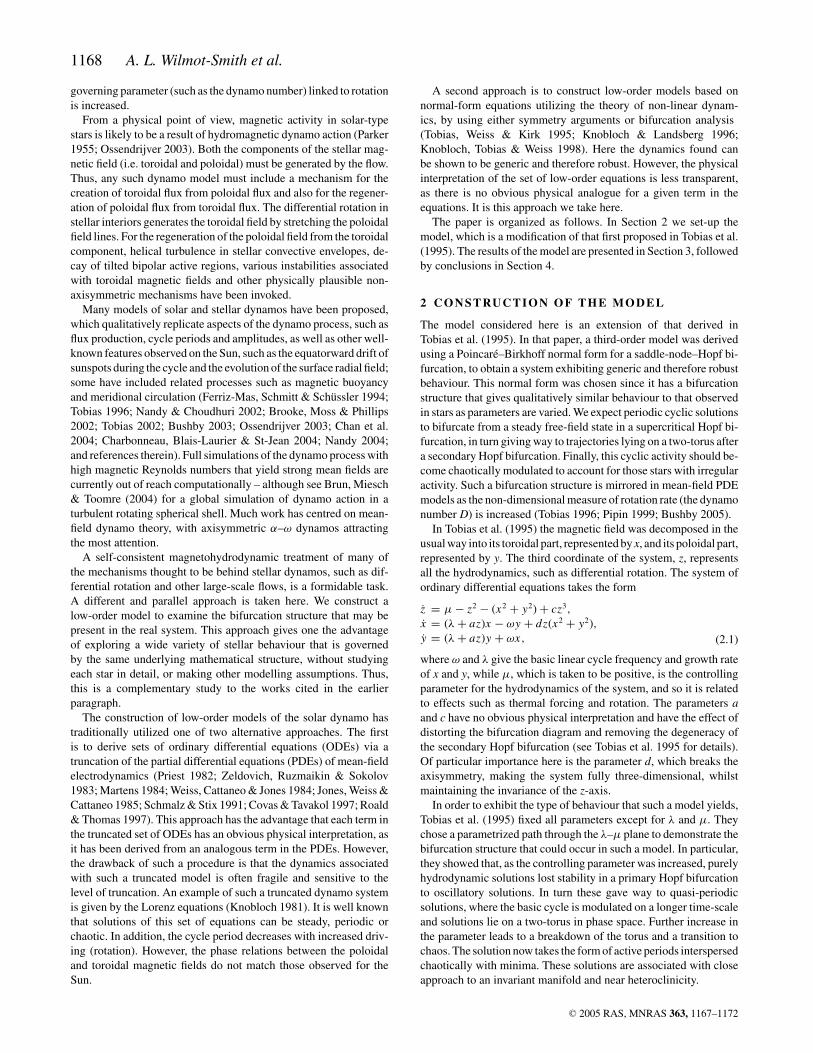
To allow us to choose a suitable path through parameter spacealong which to study solutions of (2.2), we examine the bifurcationset for the system; this is shown in Fig. 1. We see that the lineof secondary Hopf bifurcations, which for d = 0 was identical to

0

0.2

0.4

0.6

0.8

1µ

−2 2 4 6 8λ

primaryHopf

secondaryHopf secondary

Hopf

saddle-node

nodesaddle-

Figure 1. Bifurcation set for equation (2.2) with a = 3, c = −d = 0.4 andω = 10.25.

the positive µ-axis, has moved leftward in our new model (2.2). Aheteroclinic region, which is shaded in the diagram, replaces thedegenerate heteroclinic bifurcation that exists when d = 0, as inTobias et al. (1995). We have not indicated all the bifurcations lyinginside this wedge owing to the complexity of the region, some detailsof which are described in, for example, Champneys & Kirk (2004).The main dynamical features observed are described as follows.

Trajectories within this region lie on a torus, and the rotation num-ber associated with each orbit may be either rational or irrational.In the case of a rational rotation number, p/q (p, q ∈ Z), since thez-axis is invariant under the flow, the orbit will turn q times aroundthe z-axis and p times around the primary periodic orbit before clos-ing in on itself. This resonance phenomenon does not occur whenthe rotation number is irrational; in this case no point on the torusis revisited in a finite time. The resonance regions are found to beslim tongues that open out smoothly from the secondary Hopf bi-furcation, and are bounded by curves of saddle-node bifurcations ofperiodic orbits (Kirk 1991). Horseshoes are introduced into the flow,resulting from the heteroclinic crossings of the stable and unstablemanifolds of two of the fixed points, and this can lead to chaoticdynamics within the region (Kirk 1991).

To illustrate the new dynamics, we examine the model’s behaviouralong a one-parameter path in theλ–µplane, chosen so that solutionsalong the path mimic the observed stellar behaviour as rotation rateis increased. We choose the parametrization

µ = √�,

λ = 14

{[ln(�) + 1

3

]exp

( − 1100 �

)}, (3.1)

where � ∈ [0, ∞), which is similar to that used in Tobias et al.(1995). Clearly the path satisfies the requirement µ > 0. It passesthrough the primary Hopf bifurcation to the left of the µ-axis andthen through the heteroclinic region, staying close to the µ-axis(which is where the complicated dynamics occur). The path thentends back to this axis to give stable dynamo action as � → ∞.

In this section we present the numerical results obtained by inte-grating the system (2.2) using the Runge–Kutta Fehlberg numericalmethod in MAPLE. Although we can loosely think of � as represent-ing the effects of rotation on the system, we cannot link it directlywith any physical parameters such as the Rossby number. As weshall show, the behaviour of the system of equations (2.2) alongthe parametrized path (3.1) is similar to that found by Tobias et al.(1995).

For small �, all trajectories are attracted to one of the fixed pointsthat correspond to purely hydrodynamic states. Magnetic instabilitysets in at � = 1.336 × 10−2 with a primary (supercritical) Hopfbifurcation, so that periodic trajectories are apparent, a typical ex-ample of which is shown in Fig. 2. The radius of the periodic orbitgrows as � is increased, giving solutions for the magnetic field

0

0.05

0.1

0.15

x^2

100 101 102 103 104 105t

Figure 2. Magnetic activity solution for (2.2) as a function of time alongthe parametrized path (3.1) at � = 0.05. A small-amplitude oscillation ispresent, whose amplitude grows as � is increased.

C© 2005 RAS, MNRAS 363, 1167–1172

1170 A. L. Wilmot-Smith et al.

(represented here by x2) that grow in amplitude with increasing �.The period of oscillation remains approximately constant through-out, since it is controlled largely by the variable ω, with small pertur-bations to the period arising from the axisymmetry-breaking term.

−0.4−0.2

00.2

0.4z

−1−0.5

00.5

1x

−1−0.5

00.5

1

y

(a)

−0.4−0.2

00.2

0.4z

−1−0.5

00.5

1x

−1−0.5

00.5

1

y

(b)

0

0.5

1

1.5

x^2

100 102 104 106 108 110 112t

(c)

0

0.5

1

1.5

x^2

102 104 106 108 110 112 114t

(d)

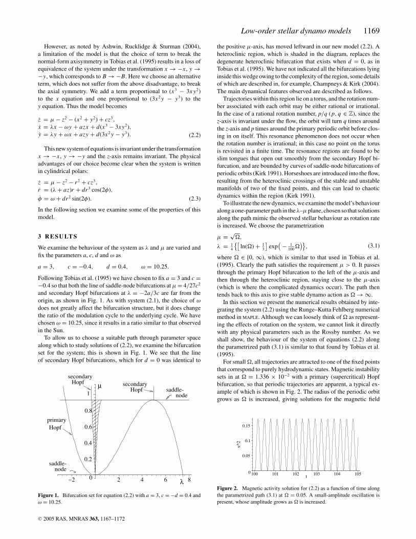
Figure 3. Solutions to (2.2) along the parametrized path (3.1). The 3Dtrajectory plot is shown for (a) the quasi-periodic solutions at � = 0.47, and(b) the frequency locking at � = 0.44. The corresponding activity cycles,represented by x2, are shown, with (c) � = 0.47 and (d) � = 0.44.

As the amplitude of the magnetic field grows, the Lorentz force be-comes important, varying periodically with half the period of thefield, as does the velocity.

At � = 0.33 (where λ < 0), the path crosses the line of thesecondary Hopf bifurcation where a torus bifurcates from the pe-riodic orbit. The solutions for x(t) and y(t), which were periodicbefore the secondary Hopf bifurcation, are now also modulatedon a longer time-scale, which results in an oscillatory magneticfield with significant amplitude variations in time. At � = 0.47, forexample, solutions are quasi-periodic, as shown in Figs 3(a) and(c). Moving along the parametrized path takes us through various

−0.2

−0.10

0.1

0.2

0.3

z

−1 −0.5 0.5 1x

(a)

−0.6−0.4−0.2

0

0.20.40.6

z−1.5 −1 −0.5 0.5 1 1.5x

(b)

−1

−0.5

0.5 z−2 −1 1 2

x

(c)

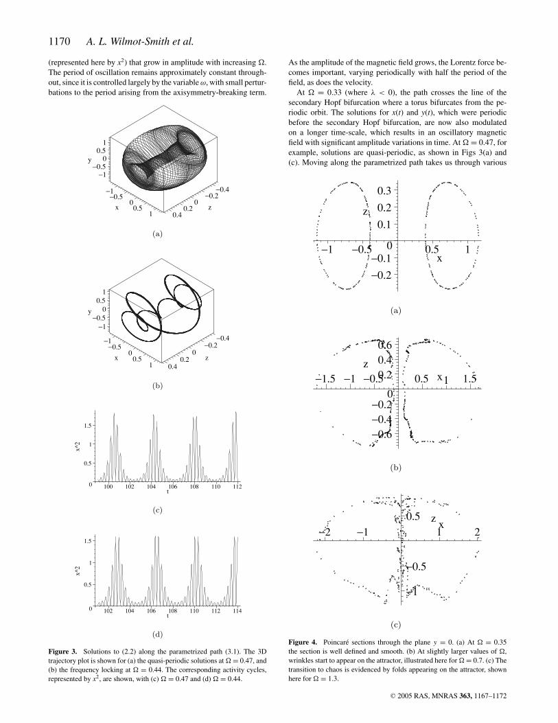
Figure 4. Poincare sections through the plane y = 0. (a) At � = 0.35the section is well defined and smooth. (b) At slightly larger values of �,wrinkles start to appear on the attractor, illustrated here for � = 0.7. (c) Thetransition to chaos is evidenced by folds appearing on the attractor, shownhere for � = 1.3.

C© 2005 RAS, MNRAS 363, 1167–1172

Low-order stellar dynamo models 1171

resonance regions, an example of which occurs at � = 0.44, asshown in Figs 3(b) and (d). The solutions for x(t) and y(t) appearto be qualitatively similar, but we see that the trajectory winds ex-actly six times around the z-axis in one period before returning toits original location. Near the frequency-locked regions where thewinding numbers are irrational but close to a rational p/q, the orbitcan spend most of its time in a phantom periodic orbit from whichit occasionally unlocks.

Quasi-periodic solutions do not persist far from the secondaryHopf bifurcation, with the resonance tongues closing off as it is ap-proached. As � is increased, the torus grows and begins to approachthe invariant z-axis. In addition the torus becomes less smooth, withfirst wrinkles, then folds developing on the attractor, an effect bestillustrated by taking Poincare sections through the plane y = 0. Weshow this in Fig. 4, where the appearance of folds on the sectionmarks a transition to chaos. The modulation of the underlying cyclein the time series for x and y becomes irregular.

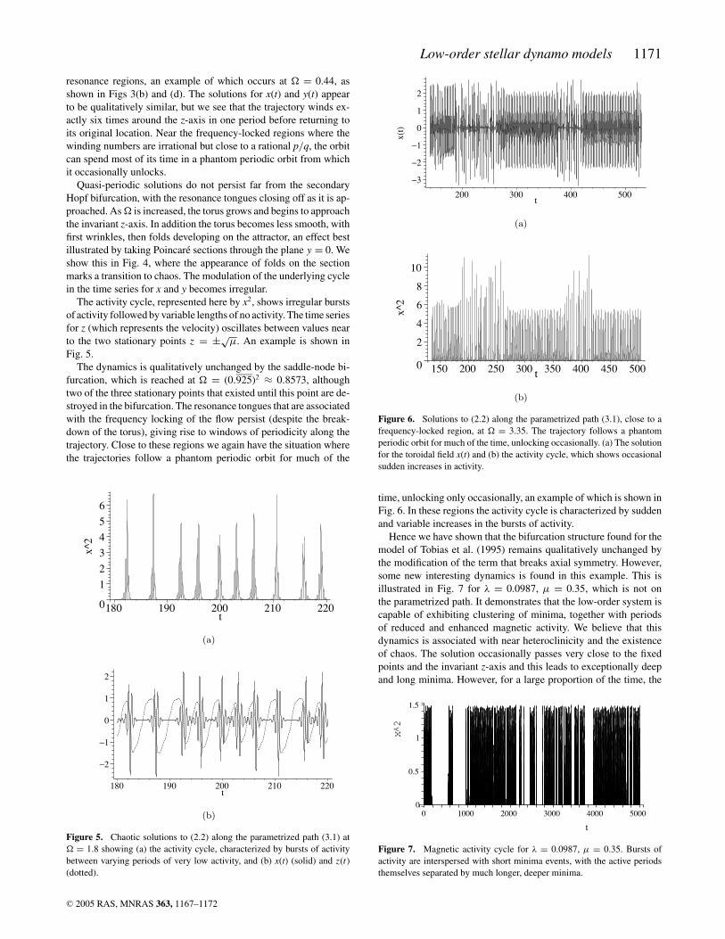
The activity cycle, represented here by x2, shows irregular burstsof activity followed by variable lengths of no activity. The time seriesfor z (which represents the velocity) oscillates between values nearto the two stationary points z = ±√

µ. An example is shown inFig. 5.

The dynamics is qualitatively unchanged by the saddle-node bi-furcation, which is reached at � = (0.925)2 ≈ 0.8573, althoughtwo of the three stationary points that existed until this point are de-stroyed in the bifurcation. The resonance tongues that are associatedwith the frequency locking of the flow persist (despite the break-down of the torus), giving rise to windows of periodicity along thetrajectory. Close to these regions we again have the situation wherethe trajectories follow a phantom periodic orbit for much of the

0

1

2

3

4

5

6

x^2

180 190 200 210 220t

(a)

−2

−1

0

1

2

180 190 200 210 220t

(b)

Figure 5. Chaotic solutions to (2.2) along the parametrized path (3.1) at� = 1.8 showing (a) the activity cycle, characterized by bursts of activitybetween varying periods of very low activity, and (b) x(t) (solid) and z(t)(dotted).

−3

−2

−1

0

1

2

x(t)

200 300 400 500t

(a)

0

2

4

6

8

10

x^2

150 200 250 300 350 400 450 500t

(b)

Figure 6. Solutions to (2.2) along the parametrized path (3.1), close to afrequency-locked region, at � = 3.35. The trajectory follows a phantomperiodic orbit for much of the time, unlocking occasionally. (a) The solutionfor the toroidal field x(t) and (b) the activity cycle, which shows occasionalsudden increases in activity.

time, unlocking only occasionally, an example of which is shown inFig. 6. In these regions the activity cycle is characterized by suddenand variable increases in the bursts of activity.

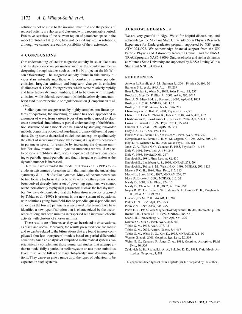
Hence we have shown that the bifurcation structure found for themodel of Tobias et al. (1995) remains qualitatively unchanged bythe modification of the term that breaks axial symmetry. However,some new interesting dynamics is found in this example. This isillustrated in Fig. 7 for λ = 0.0987, µ = 0.35, which is not onthe parametrized path. It demonstrates that the low-order system iscapable of exhibiting clustering of minima, together with periodsof reduced and enhanced magnetic activity. We believe that thisdynamics is associated with near heteroclinicity and the existenceof chaos. The solution occasionally passes very close to the fixedpoints and the invariant z-axis and this leads to exceptionally deepand long minima. However, for a large proportion of the time, the

1000

1

0.5

500040000

1.5

20000

3000

t

Figure 7. Magnetic activity cycle for λ = 0.0987, µ = 0.35. Bursts ofactivity are interspersed with short minima events, with the active periodsthemselves separated by much longer, deeper minima.

C© 2005 RAS, MNRAS 363, 1167–1172

1172 A. L. Wilmot-Smith et al.

solution is not so close to the invariant manifold and the periods ofreduced activity are shorter and clustered with a recognizable period.Extensive searches of the relevant region of parameter space in themodel of Tobias et al. (1995) have not located any similar solutions,although we cannot rule out the possibility of their existence.

4 C O N C L U S I O N S

Our understanding of stellar magnetic activity in solar-like starsand its dependence on parameters such as the Rossby number isdeepening through studies such as the H+K project at the Mt Wil-son Observatory. The magnetic activity found in this survey di-vides stars naturally into those with constant emission, periodicemission, irregular emission and long-term changes in emission(Baliunas et al. 1995). Younger stars, which rotate relatively rapidlyand have higher dynamo numbers, tend to be those with irregularemission, while older slower rotators (which have low dynamo num-bers) tend to show periodic or regular emission (Hempelmann et al.1996).

Stellar dynamos are governed by highly complex non-linear sys-tems of equations, the modelling of which has been approached ina number of ways, from various types of mean-field model to elab-orate numerical simulations. A partial understanding of the bifurca-tion structure of such models can be gained by studying low-ordermodels, consisting of coupled non-linear ordinary differential equa-tions. Using such a theoretical model one can explore qualitativelythe effect of increasing rotation by looking at a system’s behaviourin parameter space, for example by increasing the dynamo num-ber. For slow rotators (small dynamo numbers) we would expectto observe a field-free state, with a sequence of bifurcations lead-ing to periodic, quasi-periodic, and finally irregular emission as thedynamo number is increased.

Here we have extended the model of Tobias et al. (1995) to in-clude an axisymmetry-breaking term that maintains the underlyingsymmetry B → −B of stellar dynamos. Many of the parameters canbe tied loosely to physical effects; however, since the system has notbeen derived directly from a set of governing equations, we cannotrelate them directly to physical parameters such as the Rossby num-ber. We have demonstrated that the bifurcation sequence proposedby Tobias et al. (1995) is present in the new system of equations,with solutions going from field-free to periodic, quasi-periodic andchaotic as the forcing parameter is increased. Furthermore we haveidentified a new type of solution that is characterized by the occur-rence of long and deep minima interspersed with increased chaoticactivity with clusters of shorter minima.

These results are of interest as they can be related to observations,as discussed above. Moreover, the results presented here are robustand so can be related to the bifurcations that are found in more com-plicated (but less transparent) models based on partial differentialequations. Such an analysis of simplified mathematical systems canscientifically complement those numerical studies that attempt ei-ther to model fully a particular stellar system or, at a more ambitiouslevel, to solve the full set of magnetohydrodynamic dynamo equa-tions. They can even give a guide as to the types of behaviour to beexpected in such systems.

AC K N OW L E D G M E N T S

We are very grateful to Nigel Weiss for helpful discussions, andacknowledge the Montana State University Solar Physics ResearchExperience for Undergraduates program supported by NSF grantATM-0243923. We acknowledge financial support from the UKParticle Physics and Astronomy Research Council and the NASATRACE program NAS5-38099. Studies of solar and stellar dynamosat Montana State University are supported by NASA Living With aStar grant NNG05GE47G.

R E F E R E N C E S

Ashwin P., Rucklidge A. M., Sturman R., 2004, Physica D, 194, 30Baliunas S. L. et al., 1995, ApJ, 438, 269Beer J., Tobias S., Weiss N., 1998, Solar Phys., 181, 237Brooke J., Moss D., Phillips A., 2002, A&A, 395, 1013Brun A. S., Miesch M. S., Toomre J., 2004, ApJ, 614, 1073Bushby P. J., 2003, MNRAS, 342, L15Bushby P. J., 2005, Astron. Nachr., 326, 218Champneys A. R., Kirk V., 2004, Physica D, 195, 77Chan K. H., Liao X., Zhang K., Jones C., 2004, A&A, 423, L37Charbonneau P., Blais-Laurier G., St-Jean C., 2004, ApJ, 616, L183Covas E., Tavakol R., 1997, Phys. Rev. E, 55, 6641Duncan D. K. et al., 1991, ApJS, 76, 383Eddy J. A., 1976, Sci, 192, 1189Ferriz-Mas A., Schmitt D., Schussler M., 1994, A&A, 289, 949Hempelmann A., Schmitt J. H. M. M., Stepein K., 1996, A&A, 305, 284Hoyt D. V., Schatten K. H., 1996, Solar Phys., 165, 181Jones C. A., Weiss N. O., Cattaneo F., 1985, Physica D, 14, 161Kirk V., 1991, Phys. Lett. A, 154, 243Kirk V., 1993, Physica D, 66, 267Knobloch E., 1981, Phys. Lett. A, 82, 439Knobloch E., Landsberg A. S., 1996, MNRAS, 278, 294Knobloch E., Tobias S. M., Weiss N. O., 1998, MNRAS, 297, 1123Martens P. C. H., 1984, Phys. Rep., 115, 315Mestel L., Spruit H. C., 1987, MNRAS, 226, 57Moss D., Brooke J., 2000, MNRAS, 315, 521Nandy D., 2004, Solar Phys., 224, 161Nandy D., Choudhuri A. R., 2002, Sci, 296, 1671Noyes R. W., Hartmann L. W., Baliunas S. L., Duncan D. K., Vaughan A.

H., 1984, ApJ, 279, 763Ossendrijver M., 2003, A&AR, 11, 287Parker E. N., 1955, ApJ, 122, 293Pipin V. V., 1999, A&A, 346, 295Priest E. R., 1982, Solar Magnetohydrodynamics. Reidel, Dordrecht, p. 338Roald C. B., Thomas J. H., 1997, MNRAS, 288, 551Saar S. H., Brandenburg A., 1999, ApJ, 524, 295Schmalz S., Stix S., 1991, A&A, 245, 654Tobias S. M., 1996, A&A, 307, L21Tobias S. M., 2002, Astron. Nachr., 3/4, 417Tobias S. M., Weiss N. O., Kirk K., 1995, MNRAS, 273, 1150Wagner G. et al., 2001, Geophys. Res. Lett., 28, 303Weiss N. O., Cattaneo F., Jones C. A., 1984, Geophys. Astrophys. Fluid

Dyn., 30, 305Zeldovich Ia. B., Ruzmaikin A. A., Sokolov D. D., 1983, Fluid Mech. As-

trophys. Geophys., 3, 381

This paper has been typeset from a TEX/LATEX file prepared by the author.

C© 2005 RAS, MNRAS 363, 1167–1172