LOW-DIMENSIONAL OFFSHORE WAVE INPUT FOR EXTREMEEVENT QUANTIFICATION

A PREPRINT

Kenan Šehic∗Department of Applied Mathematics and Computer Science

Technical University of DenmarkDK-2800 Kgs. Lyngby, Denmark

Henrik BredmoseDepartment of Wind Energy

Technical University of DenmarkDK-2800 Kgs. Lyngby, Denmark

John D. SørensenDepartment of Civil Engineering & Department of Wind Energy

Aalborg University & Technical University of DenmarkDenmark

Mirza KaramehmedovicDepartment of Applied Mathematics and Computer Science

Technical University of DenmarkDK-2800 Kgs. Lyngby, Denmark

April 24, 2020

ABSTRACT

In offshore engineering design, nonlinear wave models are often used to propagate stochastic wavesfrom an input boundary to the location of an offshore structure. Each wave realization is typicallycharacterized by a high-dimensional input time series, and a reliable determination of the extremeevents is associated with substantial computational effort. As the sea depth decreases, extreme eventsbecome more difficult to evaluate. We here construct a low-dimensional characterization of thecandidate input time series to circumvent the search for extreme wave events in a high-dimensionalinput probability space. Each wave input is represented by a unique low-dimensional set of parametersfor which standard surrogate approximations, such as Gaussian processes, can estimate the short-termexceedance probability efficiently and accurately. We demonstrate the advantages of the new approachwith a simple shallow-water wave model based on the Korteweg-de Vries equation for which we canprovide an accurate reference solution based on the simple Monte Carlo method. We furthermoreapply the method to a fully nonlinear wave model for wave propagation over a sloping seabed.The results demonstrate that the Gaussian process can learn accurately the tail of the heavy-taileddistribution of the maximum wave crest elevation based on only 1.7% of the required Monte Carloevaluations.

Keywords sequential design · Gaussian process regression · offshore applications · dimensionality reduction · extremeevents

∗Corresponding author: kense@dtu.dk

arX

iv:2

004.

1086

1v1

[ph

ysic

s.da

ta-a

n] 2

2 A

pr 2

020

A PREPRINT - APRIL 24, 2020

1 Introduction

The occurrence of extreme events is typically quantified by a d-fold integral, called the probability of failure,

PF =

∫γ−g(θ)≤0

πd(θ)dθ, (1)

where θ ∈ Rd is the stochastic input of a limit-state function γ− g(θ), πd is the joint probability density function (PDF)for θ and g(θ) ≥ γ defines a failure event with a failure threshold γ. In the present study, the failure event is defined bya wave crest elevation g(θ) (for example, the maximum 1-hour crest elevation) exceeding a certain threshold γ. Werecognize the probability of failure, Eq. (1), as the short-term exceedance probability since the failure event is definedfor a predefined sea state. For a real design situation, the short-term probability distribution would be further integratedover the range of possible sea states to define the long-term exceedance probability. We here focus only on the efficientevaluation of the short-term exceedance probability. We define θ to be a highly dimensional vector of stochastic Fouriercoefficients that generate input waves which recreate real offshore conditions [1, 2, 3, 4].

In offshore engineering, the short-term exceedance probability, Eq. (1), is often estimated with the well-known reliabilityapproaches FORM/SORM, which are the first/second-order Taylor series approximations of the limit-state function atthe design point. However, FORM/SORM idealize the failure surface and fall short of defining multiple failure regions[5]. Additionally, as a geometrical approach, FORM/SORM do not provide error estimates. A robust alternative is thesimple Monte Carlo (MC) method [6]. It does not depend on the dimension of the input and can find multiple designpoints for almost any numerical model. In this framework, the short-term exceedance probability, Eq. (1), is definedas the sample mean of the indicator function I(θ), where I(θ) = 1 if g(θ) ≥ γ and I(θ) = 0 otherwise. The idea isto compute N blind samples of the numerical model and estimate the sample mean. While being a straightforwardapproach to implement, MC is infeasible in conjunction with expensive numerical models due to the slow convergencerate O(N−1/2). As we are only able to approximate the sample mean Eq. (1), we employ the mean squared errormeasure to define a sufficient number of evaluations N for a prescribed relative error [6]. For example, the responsevalue of an exceedance probability of 2 · 10−3 with the relative error less than 0.1 requires at least N = 5 · 104

evaluations. A numerical model which needs 1 minute to compute would require approximately 35 days to find theshort-term exceedance probability. Therefore, surrogate methods such as Polynomial Chaos expansion [7] and Gaussian(Kriging) process [8] are usually proposed to define a low-cost surrogate for the numerical model using a small numberof evaluations. The low-cost surrogate is then employed to approximate efficiently the short-term exceedance probability.However, the requirements for standard surrogate methods typically exponentially increase with the dimension dueto the curse of dimensionality [9]. For high-dimensional problems, as the one considered in this paper, this approachbecomes infeasible.

Alternative approaches consider only the statistical characteristics of extreme events such as extreme value theorems [10]and large deviations theory [11, 12]. However, these methods have essential limitations requiring various extrapolationschemes due to the insufficient size of the sample set, and they therefore cannot always explain the non-trivial shapeof the tail. The Fokker-Planck equation (FPE) [13] incorporates into the estimation the governing dynamical systemof the model, as well as the stochastic nature of extreme events. However, even in low-dimensional cases, the FPE isprohibitively difficult to solve.

Mohamad et al. [14] proposed a sequential sampling strategy based on Gaussian process regression and statisticalproperties of extreme events. They formulated an optimization process that selected the most informative designpoint according to the log-L2 criterion, which eventually reduce the uncertainties in the prediction of extreme events.To avoid the curse of dimensionality, their numerical implementation is low-dimensional. For a wave-propagationapplication, they characterize the input condition by just two parameters, namely wave group length and amplitude.Although the wave group parameters are good indicators of extreme wave events [15, 16, 17, 18, 19], the propagationover long distances from the generation boundary makes single-group characteristics less relevant in the general case.Other options would be to employ standard dimensionality reduction tools such as principal component analysis (PCA)[20], partial least squares regression (PLS) [21, 22], active-subspace analysis [9, 16], or autoencoders [23]. However,these standard dimensionality reduction tools may provide inefficient reduction in offshore applications or suffer fromexpensive and intrusive implementation.

To improve on this, we propose a low-dimensional classification representation of the high-dimensional Gaussian input.Based on the input sample set of the predefined input sea state, we classify the wave input by classification parametersunique for each time series. The classification parameters are now the low-dimensional design input parameters forGaussian process regression. To reduce the prediction uncertainties for extreme events, we select the most informativedesign points from the input Gaussian evaluations based on the probability of misclassification [8]. We test our approachin two numerical experiments. The first is based on the Korteweg-de Vries equation, which is a simple shallow-waterwave model for which we can generate the reference solution with the simple Monte Carlo method. The second case is

2

A PREPRINT - APRIL 24, 2020

fully nonlinear wave propagation over a sloping seabed, computed with the OceanWave3D model [24]. We select theclassification parameters heuristically, and view this paper as initial work on the low-dimensional representation ofoffshore wave input, or generally of input time-series for any system.

Section 2 covers Gaussian process regression in general. We introduce the low-dimensional representation of inputtime series in Section 3, and present the numerical experiments in Section 4. There, we demonstrate that the low-dimensional representation based on our classification parameters is suitable for the Gaussian process design andefficient quantification of extreme events. We present our conclusions in Section 5.

2 Gaussian process regression

When the numerical cost of a model prohibits the quantification of the involved uncertainties, it is natural to try toconstruct a surrogate model, a low-cost replacement based on a small number of evaluations NGP of the original model.In this work we use Gaussian or Kriging process regression (GP), which employs the Gaussian distribution over atraining set based on a Bayesian approximation [25]. The training set, S = (θi, g(θi)), includes the matrix of the inputparameters X = (θi) ∈ RNGP×d and the corresponding evaluations of a numerical model Y = (Yi = g(θi)) ∈ RNGP×1.For an arbitrary smooth function g, we define a Gaussian process approximation by [25, 8]

g(θ) ≈ g(θ) = βT · fT(θ) + σ2Z(θ, ωz), (2)where βT · fT(θ) is the trend, σ2 is the variance of the Gaussian process, and Z(θ, ωz) is a zero-mean, unit-variancestationary Gaussian process with ωz ∈ Ω as an elementary event in the probability space (Ω,F ,P). The trend fT (θ)describes the global behavior of the training set, and is defined using simple regression. The complexity of the Gaussianprocess Z is described by a stationary kernel matrix Kij = K(|θi − θj |; Θ), where Θ are the hyperparameters suchas the overall correlation of the samples or the smoothness of the training set. The performance of the GP regressiondepends highly on the selection of the kernel function. For example, a periodic kernel may be best suited for a periodictraining set. We define the regression parameters β and σ2 based on generalized least-squares regression [8]. Thehyperparameters Θ for the kernel matrix Kij are found using maximum likelihood estimation. A typical challenge is toselect an optimal size NGP of the training set. Gramacy and Apley [26] propose to select the training size by addingobservations until a certain mean squared predictive error is no longer fulfilled. Once the GP model is trained, weestimate for an arbitrary input sample θ∗ the prediction µg(θ∗) and the variance (i.e., an uncertainty measure) σ2

g(θ∗)via [25, 8]

µg(θ∗) = fT(θ∗) · β + k(θ∗)TK−1(Y − FTβ), (3)

and

σ2g(θ∗) = σ2

(1−

⟨fT(θ∗)T k(θ∗)T

⟩[0 FTTFT K

]−1 [fT(θ∗)k(θ∗)

]). (4)

Here k(θ∗) is the correlation between the arbitrary input sample and the rest of the samples within the training set, andFT is the information matrix regarding the GP trend.

2.1 Sequential Uncertainty Reduction for Extreme Events

Gaussian process regression provides the posterior distribution, based on the moments (3) and (4), which describes thequality of the predictions and, in general, the performance of the surrogate model. An arbitrary Gaussian predictionµg(θ

∗) and the corresponding standard deviation σg(θ∗) define the confidence interval (CI) [8, 25]

µ±CI(θ

∗) = µg(θ∗)± α · σg(θ∗), (5)

with confidence level α. For example, α = 1.96 for 95% confidence, and 95% of the area of the normal distribution iswithin 1.96 standard deviations. Narrower confidence intervals mean more confidence in the predictions and generallyin the performance of the surrogate model, under the assumption that the limit-state function is smooth. However, asignificantly narrow CI can still over/under-predict a highly nontrivial response, because Gaussian process regressionis a design method. The training set and the initial design may not be sufficient to accurately describe a complicatedfunction. The application is not straightforward and should be employed carefully with an understanding of thenumerical model and the data itself. Hence, the idea is to sequentially design numerical experiments θ∗ for trainingwhile exploring optimally the probability space (i.e., using a learning function) to create an optimal Gaussian process.Mohamad et al. [14] proposed a sequential design utilizing the log-L2 distance between the upper and lower bound ofCI to reduce uncertainties for extreme events. Schöbi et al. [8] used the probability of misclassification to define which

3

A PREPRINT - APRIL 24, 2020

numerical experiments θ∗ are close to a predefined failure threshold or are poorly predicted. We find this sufficient forour analysis.

As the probability of failure essentially involves a binary classification, with 1 for failure and 0 otherwise, themisclassification of predictions based on the first two moments and on the failure threshold γ is a natural option forGaussian process regression. We write for the probability of misclassification PM [8]

PM (θ∗) = Φ

(−|µg(θ

∗)− γ|σg(θ∗)

). (6)

Here, the U -function (the learning function) is the fraction in the argument in (6). It is recognized as the reliabilityindex attached to PM with Φ as the cumulative distribution function of the standard normal distribution. Small valuesof the U -function reveal the samples θ∗ that are close to the predefined failure threshold γ or have high uncertaintiesin predictions. Therefore, to improve the training set, we select the most informative design points, i.e., the inputparameters θ∗ with the smallest U -values, based on the generated samples SMC = θ1, · · · , θN ∈ RN×d. Thisproduces a Gaussian process designed specially for extreme events. The procedure is iterative, as we add more U -baseddesign points θ∗ until an error measure based on the confidence interval for the failure level drops below some prescribedthreshold.

Algorithm 1 Gaussian discrete learning with the U -function1: procedure U -GP(θ ∈ Rd- the input parameters, g - the numerical model, S = (θi, g(θi)) ∈ RNGP×d - the

training set, SMC = θ1, · · · , θN ∈ RN×d - the generated samples, γ - the failure threshold)2: Train a Gaussian process on the training set S.3: Use the trained GP to estimate the first two moments for the generated samples SMC following Eq. (3) and

Eq. (4).4: Estimate the confidence interval based on SMC with Eq. (5) and quantify the exceedance probabilities PF andP±F as the sample means of the indicator function based on the failure threshold γ.

5: Evaluate the error measure εγ by Eq. (7) for the failure threshold γ.6: repeat7: For each generated sample θ∗ from the set SMC, estimate the U -value based on the U -function and the

failure threshold γ,

U(θ∗) =|µg(θ∗)− γ|σg(θ∗)

.

8: Select an arbitrary number of samples θ∗ ∈ RNU×d that achieve minimal U -values and evaluate a numericalmodel g(θ∗).

9: Include the pair (θ∗, g(θ∗)) within the training set S.10: Repeat Lines 2-5.11: until For a prescribed error threshold ξ: εγ ≤ ξ.12: end procedure

The procedure is described in more detail in Algorithm 1. It can be seen as discrete learning, since we rely on thegenerated samples SMC. The optimal approach is to select the sample that maximizes the probability of misclassificationor minimizes the U -function based on the trained GP. As the trained GP is a surrogate model, the optimization procedureis low-cost. However, for our approach, which uses classification parameters, we can only build the procedure on thegenerated samples. The error measure, a stopping criterion, is defined as [8]

εγ =|P+F − P

−F |

PF, (7)

where the exceedance probabilities PF and P±F are estimated as the sample means of the indicator function by the

simple Monte Carlo method based on the generated samples SMC. The exceedance probabilities P±F involve the upper

and lower bounds of the confidence interval. The error measure (7) usually ranges between 0.5 and 2 [8]. It dependson the final failure level and the accuracy requirement. If the error measure is not achieved (i.e., εγ > ξ), the discretelearning converges to the simple Monte Carlo estimation of the generated samples.

4

A PREPRINT - APRIL 24, 2020

3 Low-dimensional representation

When the input dimension d exceeds extreme values, e.g., d = 100, it is required to define a larger training set NGP

based on the factorial design. However, the computation of the Gaussian process becomes impractical as anNGP×NGP

kernel matrix needs to be inverted several times to make an arbitrary prediction, which costs O(N3GP). Therefore, the

literature on Gaussian process regression typically covers low-dimensional numerical implementations [15, 14].

We define the input parameters within a high-dimensional probability space to recreate the environmental conditionsaccurately. The boundary condition, which we note as the wave input at x = 0, is defined as a Fourier series withmulti-dimensional random coefficients drawn from the standard normal distribution [27]

η(x, t) =

d/2∑j=1

√S(fj) ·∆f

[Aj cos(2πfjt− kjx) +Bj sin(2πfjt− kjx)

]. (8)

Here S(fj) is the wave energy spectrum, i.e., JONSWAP [4], fj are wave frequencies, kj are the wavenumbers and Ajand Bj are random variables drawn from the standard normal distribution N (0, 1). In this paper, the input parametersAj and Bj are written θ = (A1, . . . , Ad/2, B1, . . . , Bd/2) ∈ Rd. The dimensionality d is based on the frequency step∆f = 1/T , where T is the time duration of the numerical simulation. For example, for 1-hour wave propagation wehave d = 1802. This is an extreme problem of uncertainty quantification due to the curse of dimensionality, whichtypically makes the problem complexity grow exponentially with the dimension. Also, in offshore applications thenumerical model usually imposes intensive computation and is to be employed only a limited number of times. [14]

We propose a novel approach to quantify extreme events in otherwise infeasible situations. The low-dimensionalrepresentation approach classifies initial surface elevations based on non-dimensional classification parameters as eachsurface elevation (i.e. time-series) has a unique set of characteristics. We change the problem set from the extremehigh-dimensional Fourier coefficients θ to the low-dimensional representation based on the classification parameters K.In the present study, we employ standard statistical measures [28] to classify the wave input Eq. (8). Following thesimple Monte Carlo requirement for the exceedance probability of 2 · 10−3, we first generate N = 5 · 104 initial surfaceelevations for the time duration T , and classify the wave input heuristically based on 10 classification parameters K1−10

(scaled by their maximum values) as [28]

• K1 - the maximum crest elevation at x = 0.• K2 - the wave input variance - second moment σ2.• K3 - the wave input skewness - third moment.• K4 - the wave input kurtosis - fourth moment.• K5 - the wave input root mean square (RMS).• K6 - the wave input approximate entropy, which measures complexity.• K7 - the wave input percentile for 50%.• K8 - the wave input percentile for 75%.• K9 - the wave input percentile for 90%.• K10 - the wave input mode as the most frequent value within the surface elevation.

4 Numerical experiments

We illustrate the proposed approach on two offshore problems. The first example uses the modified Kortweg-de Vriesequation (KdV22) [16]. The second application, involving a simple OceanWave3D benchmark with wave propagationover a slope [29], demonstrates the applicability of the proposed classification approach to a fully nonlinear model. Asthe computations are intensive, the quantification of extreme events using standard methods is infeasible. Generally, weassume that the computational budget is limited.

The quantity of interest is the maximum crest elevation ηmax at the reference location x∗ for an offshore structure,

ηmax = maxη(x∗, t), 0 ≤ t ≤ T. (9)

The objective is to estimate the short-term exceedance probability for ηmax based on a predefined sea state. For bothcases, we employ the JONSWAP spectrum, which is typically used for extreme events analyses. Due to the computationlimitations, we employ short numerical simulations to examine the advantages and the disadvantages of our approach.The calculations are executed on a personal laptop with Intel Core i5-6200U CPU @ 2.30GHz × 4.

5

A PREPRINT - APRIL 24, 2020

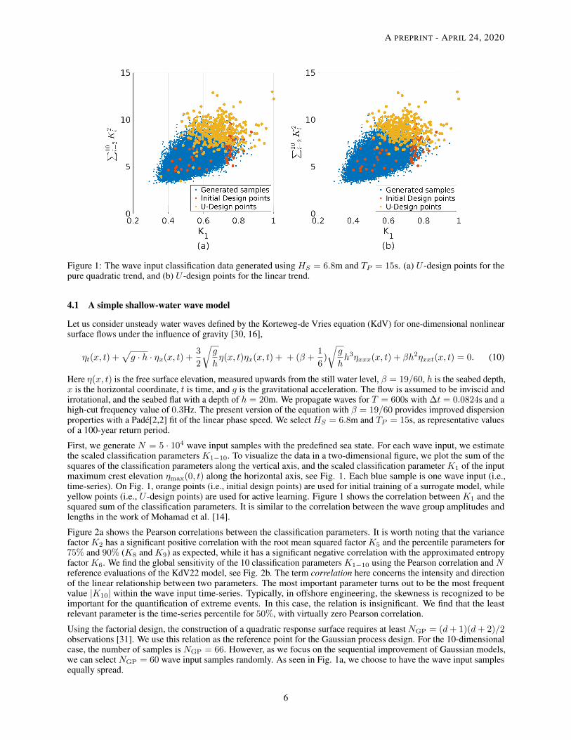
Figure 1: The wave input classification data generated using HS = 6.8m and TP = 15s. (a) U -design points for thepure quadratic trend, and (b) U -design points for the linear trend.

4.1 A simple shallow-water wave model

Let us consider unsteady water waves defined by the Korteweg-de Vries equation (KdV) for one-dimensional nonlinearsurface flows under the influence of gravity [30, 16],

ηt(x, t) +√g · h · ηx(x, t) +

3

2

√g

hη(x, t)ηx(x, t) + + (β +

1

6)

√g

hh3ηxxx(x, t) + βh2ηxxt(x, t) = 0. (10)

Here η(x, t) is the free surface elevation, measured upwards from the still water level, β = 19/60, h is the seabed depth,x is the horizontal coordinate, t is time, and g is the gravitational acceleration. The flow is assumed to be inviscid andirrotational, and the seabed flat with a depth of h = 20m. We propagate waves for T = 600s with ∆t = 0.0824s and ahigh-cut frequency value of 0.3Hz. The present version of the equation with β = 19/60 provides improved dispersionproperties with a Padé[2,2] fit of the linear phase speed. We select HS = 6.8m and TP = 15s, as representative valuesof a 100-year return period.

First, we generate N = 5 · 104 wave input samples with the predefined sea state. For each wave input, we estimatethe scaled classification parameters K1−10. To visualize the data in a two-dimensional figure, we plot the sum of thesquares of the classification parameters along the vertical axis, and the scaled classification parameter K1 of the inputmaximum crest elevation ηmax(0, t) along the horizontal axis, see Fig. 1. Each blue sample is one wave input (i.e.,time-series). On Fig. 1, orange points (i.e., initial design points) are used for initial training of a surrogate model, whileyellow points (i.e., U -design points) are used for active learning. Figure 1 shows the correlation between K1 and thesquared sum of the classification parameters. It is similar to the correlation between the wave group amplitudes andlengths in the work of Mohamad et al. [14].

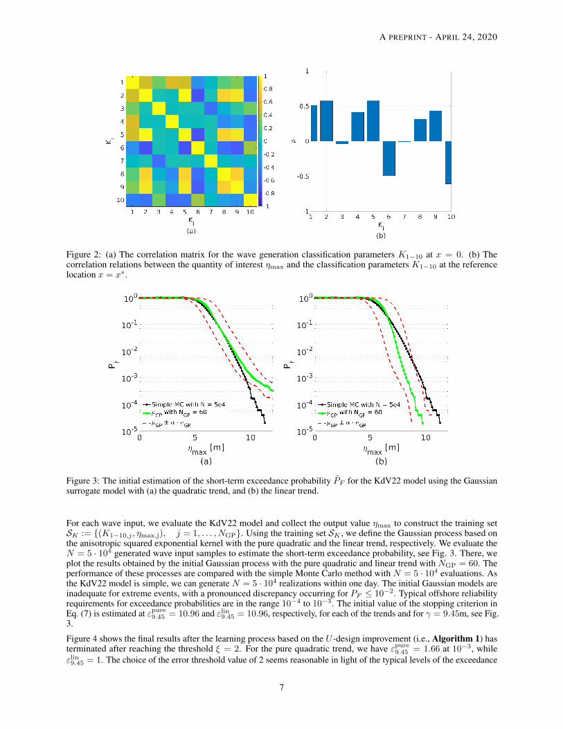
Figure 2a shows the Pearson correlations between the classification parameters. It is worth noting that the variancefactor K2 has a significant positive correlation with the root mean squared factor K5 and the percentile parameters for75% and 90% (K8 and K9) as expected, while it has a significant negative correlation with the approximated entropyfactor K6. We find the global sensitivity of the 10 classification parameters K1−10 using the Pearson correlation and Nreference evaluations of the KdV22 model, see Fig. 2b. The term correlation here concerns the intensity and directionof the linear relationship between two parameters. The most important parameter turns out to be the most frequentvalue |K10| within the wave input time-series. Typically, in offshore engineering, the skewness is recognized to beimportant for the quantification of extreme events. In this case, the relation is insignificant. We find that the leastrelevant parameter is the time-series percentile for 50%, with virtually zero Pearson correlation.

Using the factorial design, the construction of a quadratic response surface requires at least NGP = (d+ 1)(d+ 2)/2observations [31]. We use this relation as the reference point for the Gaussian process design. For the 10-dimensionalcase, the number of samples is NGP = 66. However, as we focus on the sequential improvement of Gaussian models,we can select NGP = 60 wave input samples randomly. As seen in Fig. 1a, we choose to have the wave input samplesequally spread.

6

A PREPRINT - APRIL 24, 2020

Figure 2: (a) The correlation matrix for the wave generation classification parameters K1−10 at x = 0. (b) Thecorrelation relations between the quantity of interest ηmax and the classification parameters K1−10 at the referencelocation x = x∗.

Figure 3: The initial estimation of the short-term exceedance probability PF for the KdV22 model using the Gaussiansurrogate model with (a) the quadratic trend, and (b) the linear trend.

For each wave input, we evaluate the KdV22 model and collect the output value ηmax to construct the training setSK := (K1−10,j , ηmax,j), j = 1, . . . , NGP. Using the training set SK , we define the Gaussian process based onthe anisotropic squared exponential kernel with the pure quadratic and the linear trend, respectively. We evaluate theN = 5 · 104 generated wave input samples to estimate the short-term exceedance probability, see Fig. 3. There, weplot the results obtained by the initial Gaussian process with the pure quadratic and linear trend with NGP = 60. Theperformance of these processes are compared with the simple Monte Carlo method with N = 5 · 104 evaluations. Asthe KdV22 model is simple, we can generate N = 5 · 104 realizations within one day. The initial Gaussian models areinadequate for extreme events, with a pronounced discrepancy occurring for PF ≤ 10−2. Typical offshore reliabilityrequirements for exceedance probabilities are in the range 10−4 to 10−3. The initial value of the stopping criterion inEq. (7) is estimated at εpure9.45 = 10.96 and εlin9.45 = 10.96, respectively, for each of the trends and for γ = 9.45m, see Fig.3.

Figure 4 shows the final results after the learning process based on the U -design improvement (i.e., Algorithm 1) hasterminated after reaching the threshold ξ = 2. For the pure quadratic trend, we have εpure9.45 = 1.66 at 10−3, whileεlin9.45 = 1. The choice of the error threshold value of 2 seems reasonable in light of the typical levels of the exceedance

7

A PREPRINT - APRIL 24, 2020

Figure 4: The final estimation of the short-term exceedance probability PF for the KdV22 model using the Gaussiansurrogate model with (a) the quadratic trend, and (b) the linear trend.

Method PF = 10−3 P+F = 10−3 PF = 10−4 P+

F = 10−4

Simple MC 9.48 - 10.48 -Pure Quadratic 9.38 9.67 10.48 10.54

Linear 9.22 9.55 10.42 10.54

Table 1: Estimation of the maximum wave crest ηmax [m] using Gaussian process regression with the U -function forthe KdV22 model and different exceedance levels.

probabilities (10−4 or 10−3). The pure quadratic trend requires more evaluations than the linear trend. However, theperformance of the pure quadratic trend is better, with the mean squared error (MSE) less than 4 · 10−4, while for thelinear trend the MSE is less than 10−3. By visually inspecting Fig. 4 and Table 1, it is observed that the model with thepure quadratic trend performs better. The total number of evaluations generated by the KdV22 for the pure quadratictrend is Npure

GP = 434 and for the linear trend N linGP = 400, which is around 0.87% of the total number of simple Monte

Carlo evaluations. Mostly, the design samples are closer to the events with higher peaks, see Fig. 1. The simple MonteCarlo estimations are accurately recreated for extreme events with significant differences for PF > 10−3.

4.2 Application to fully nonlinear wave propagation over a slope

We next apply the classification approach with active learning to compute the short-term exceedance probability forwave propagation over a slope with a fully nonlinear model, OceanWave3D [24]. OceanWave3D is a finite differencepotential flow solver based on the Laplace equation with kinematic and dynamic free surface boundary conditions. Anad hoc wave breaking filter is included within the model. A complete derivation of the equations can be found in [32].

We establish our numerical experiment on the benchmark example of OceanWave3D defined for random wavesover a slope [29]. MATLAB codes for this numerical experiment can be found at https://github.com/ksehic/OCW3D-F90-UQProbe in the folder UQ− Packages. The sea state parameters for the JONSWAP spectrum areHS = 4m and TP = 9s. The computation is additionally simplified as it includes 137 cells with a time duration of256 seconds and 800 meters of the spatial domain. The initial sea depth is 50m and gradually decreases to the shallowregion of 15m. The reference location is at the sea depth of approximately 30m, see Fig. 5a. Figure 5b shows thevariance estimations for different spatial locations using the initial runs of OceanWave3D. We choose the referencelocation for the short-term exceedance probability PF with the highest estimated variance. It is interesting to notice thatthe most uncertain location for this example and data is at the sea depth of h ≈ 30m, which is a depth reduction of 40%.

8

A PREPRINT - APRIL 24, 2020

Figure 5: (a) Illustration of the sloping seabed with the reference location as the blue line. (b) The expectation of thesquared deviation of ηmax from its mean i.e. the variance for each spatial position.

Figure 6: The wave generation classification data generated based on HS = 4m and TP = 9s with (a) initial trainingset N0, and (b) additional U -samples NU for γ = 4m.

The procedure is the same as previously described for the KdV22 shallow-water model. First, we generate and classifyN = 5 · 104 wave input samples with the predefined sea state (HS = 4m and TP = 9s) using K1−10, see Fig. 6. Todefine the training set, we randomly select initial NGP = 60 wave input samples for which we evaluate OceanWave3D,see Fig. 6a. Using this training set, we define the Gaussian process with the anisotropic squared exponential kernelfunction based on the pure quadratic regression. Next, we estimate the short-term exceedance probability as the samplemean with the indicator function using N generated samples, see Fig. 7a. Initially, we need to select a failure thresholdfor a numerical model and active learning. Thus, we select the failure threshold γ = 4m as HS . The initial errormeasure Eq. (7) attains the value ε4 = 5.4, see Table 2. This error measure is in this case too optimistic, in that theconfidence interval is significantly narrowed with the error measure close to the predefined stopping criterion of ξ = 2.It is a clear example that one should consider the confidence interval of a Gaussian process with skepticism. We can seein Fig. 7a that the tail of the distribution PF ≥ 10−2 is extremely heavy. The prediction is similar to the initial Gaussianprediction of the KdV22 model, see Fig. 3, which diverges significantly from its reference solution. If the predictionis true, additional carefully selected new wave input samples can only improve the stability of the Gaussian process.However, when the Gaussian process starts to learn and explore the probability space actively, the error measure ε4

9

A PREPRINT - APRIL 24, 2020

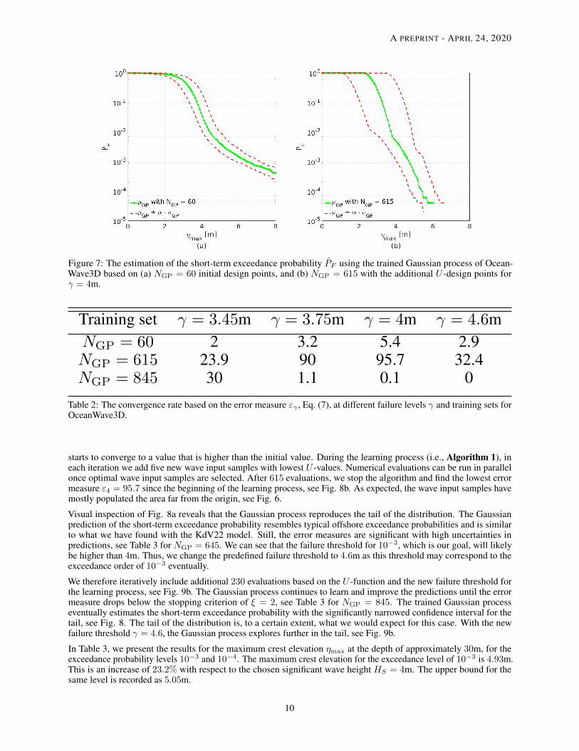
Figure 7: The estimation of the short-term exceedance probability PF using the trained Gaussian process of Ocean-Wave3D based on (a) NGP = 60 initial design points, and (b) NGP = 615 with the additional U -design points forγ = 4m.

Training set γ = 3.45m γ = 3.75m γ = 4m γ = 4.6mNGP = 60 2 3.2 5.4 2.9NGP = 615 23.9 90 95.7 32.4NGP = 845 30 1.1 0.1 0

Table 2: The convergence rate based on the error measure εγ , Eq. (7), at different failure levels γ and training sets forOceanWave3D.

starts to converge to a value that is higher than the initial value. During the learning process (i.e., Algorithm 1), ineach iteration we add five new wave input samples with lowest U -values. Numerical evaluations can be run in parallelonce optimal wave input samples are selected. After 615 evaluations, we stop the algorithm and find the lowest errormeasure ε4 = 95.7 since the beginning of the learning process, see Fig. 8b. As expected, the wave input samples havemostly populated the area far from the origin, see Fig. 6.

Visual inspection of Fig. 8a reveals that the Gaussian process reproduces the tail of the distribution. The Gaussianprediction of the short-term exceedance probability resembles typical offshore exceedance probabilities and is similarto what we have found with the KdV22 model. Still, the error measures are significant with high uncertainties inpredictions, see Table 3 for NGP = 645. We can see that the failure threshold for 10−3, which is our goal, will likelybe higher than 4m. Thus, we change the predefined failure threshold to 4.6m as this threshold may correspond to theexceedance order of 10−3 eventually.

We therefore iteratively include additional 230 evaluations based on the U -function and the new failure threshold forthe learning process, see Fig. 9b. The Gaussian process continues to learn and improve the predictions until the errormeasure drops below the stopping criterion of ξ = 2, see Table 3 for NGP = 845. The trained Gaussian processeventually estimates the short-term exceedance probability with the significantly narrowed confidence interval for thetail, see Fig. 8. The tail of the distribution is, to a certain extent, what we would expect for this case. With the newfailure threshold γ = 4.6, the Gaussian process explores further in the tail, see Fig. 9b.

In Table 3, we present the results for the maximum crest elevation ηmax at the depth of approximately 30m, for theexceedance probability levels 10−3 and 10−4. The maximum crest elevation for the exceedance level of 10−3 is 4.93m.This is an increase of 23.2% with respect to the chosen significant wave height HS = 4m. The upper bound for thesame level is recorded as 5.05m.

10

A PREPRINT - APRIL 24, 2020

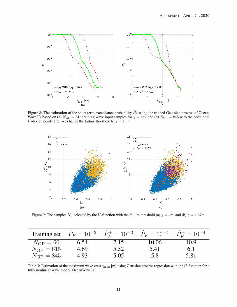
Figure 8: The estimation of the short-term exceedance probability PF using the trained Gaussian process of Ocean-Wave3D based on (a) NGP = 615 training wave input samples for γ = 4m, and (b) NGP = 845 with the additionalU -design points after we change the failure threshold to γ = 4.6m.

Figure 9: The samples NU selected by the U -function with the failure threshold (a) γ = 4m, and (b) γ = 4.67m.

Training set PF = 10−3 P+F = 10−3 PF = 10−4 P+

F = 10−4

NGP = 60 6.54 7.15 10.06 10.9NGP = 615 4.69 5.52 5.41 6.1NGP = 845 4.93 5.05 5.8 5.81

Table 3: Estimation of the maximum wave crest ηmax [m] using Gaussian process regression with the U -function for afully nonlinear wave model, OceanWave3D.

11

A PREPRINT - APRIL 24, 2020

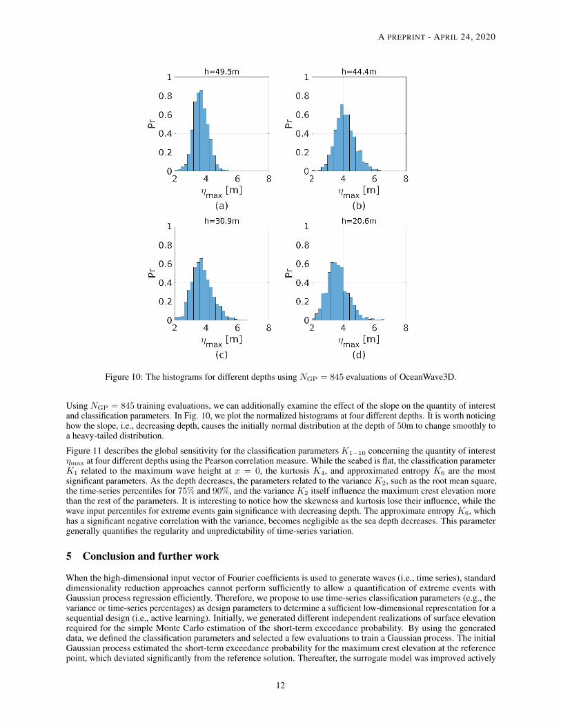
Figure 10: The histograms for different depths using NGP = 845 evaluations of OceanWave3D.

Using NGP = 845 training evaluations, we can additionally examine the effect of the slope on the quantity of interestand classification parameters. In Fig. 10, we plot the normalized histograms at four different depths. It is worth noticinghow the slope, i.e., decreasing depth, causes the initially normal distribution at the depth of 50m to change smoothly toa heavy-tailed distribution.

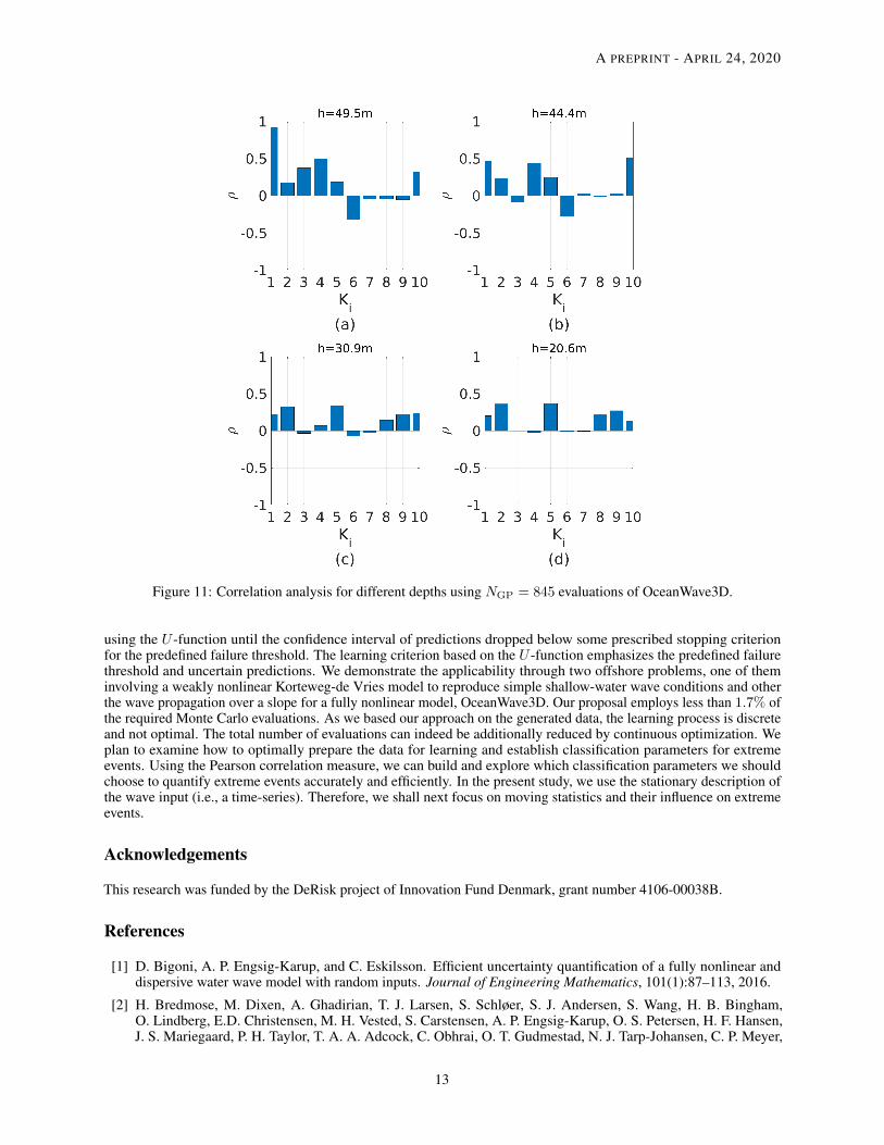
Figure 11 describes the global sensitivity for the classification parameters K1−10 concerning the quantity of interestηmax at four different depths using the Pearson correlation measure. While the seabed is flat, the classification parameterK1 related to the maximum wave height at x = 0, the kurtosis K4, and approximated entropy K6 are the mostsignificant parameters. As the depth decreases, the parameters related to the variance K2, such as the root mean square,the time-series percentiles for 75% and 90%, and the variance K2 itself influence the maximum crest elevation morethan the rest of the parameters. It is interesting to notice how the skewness and kurtosis lose their influence, while thewave input percentiles for extreme events gain significance with decreasing depth. The approximate entropy K6, whichhas a significant negative correlation with the variance, becomes negligible as the sea depth decreases. This parametergenerally quantifies the regularity and unpredictability of time-series variation.

5 Conclusion and further work

When the high-dimensional input vector of Fourier coefficients is used to generate waves (i.e., time series), standarddimensionality reduction approaches cannot perform sufficiently to allow a quantification of extreme events withGaussian process regression efficiently. Therefore, we propose to use time-series classification parameters (e.g., thevariance or time-series percentages) as design parameters to determine a sufficient low-dimensional representation for asequential design (i.e., active learning). Initially, we generated different independent realizations of surface elevationrequired for the simple Monte Carlo estimation of the short-term exceedance probability. By using the generateddata, we defined the classification parameters and selected a few evaluations to train a Gaussian process. The initialGaussian process estimated the short-term exceedance probability for the maximum crest elevation at the referencepoint, which deviated significantly from the reference solution. Thereafter, the surrogate model was improved actively

12

A PREPRINT - APRIL 24, 2020

Figure 11: Correlation analysis for different depths using NGP = 845 evaluations of OceanWave3D.

using the U -function until the confidence interval of predictions dropped below some prescribed stopping criterionfor the predefined failure threshold. The learning criterion based on the U -function emphasizes the predefined failurethreshold and uncertain predictions. We demonstrate the applicability through two offshore problems, one of theminvolving a weakly nonlinear Korteweg-de Vries model to reproduce simple shallow-water wave conditions and otherthe wave propagation over a slope for a fully nonlinear model, OceanWave3D. Our proposal employs less than 1.7% ofthe required Monte Carlo evaluations. As we based our approach on the generated data, the learning process is discreteand not optimal. The total number of evaluations can indeed be additionally reduced by continuous optimization. Weplan to examine how to optimally prepare the data for learning and establish classification parameters for extremeevents. Using the Pearson correlation measure, we can build and explore which classification parameters we shouldchoose to quantify extreme events accurately and efficiently. In the present study, we use the stationary description ofthe wave input (i.e., a time-series). Therefore, we shall next focus on moving statistics and their influence on extremeevents.

Acknowledgements

This research was funded by the DeRisk project of Innovation Fund Denmark, grant number 4106-00038B.

References

[1] D. Bigoni, A. P. Engsig-Karup, and C. Eskilsson. Efficient uncertainty quantification of a fully nonlinear anddispersive water wave model with random inputs. Journal of Engineering Mathematics, 101(1):87–113, 2016.

[2] H. Bredmose, M. Dixen, A. Ghadirian, T. J. Larsen, S. Schløer, S. J. Andersen, S. Wang, H. B. Bingham,O. Lindberg, E.D. Christensen, M. H. Vested, S. Carstensen, A. P. Engsig-Karup, O. S. Petersen, H. F. Hansen,J. S. Mariegaard, P. H. Taylor, T. A. A. Adcock, C. Obhrai, O. T. Gudmestad, N. J. Tarp-Johansen, C. P. Meyer,

13

A PREPRINT - APRIL 24, 2020

J. R. Krokstad, L. Suja-Thauvin, and T. D. Hanson. DeRisk — accurate prediction of ULS wave loads. Outlookand First Results. Energy Procedia, 90:379–387, 2016.

[3] A. Ghadirian and H. Bredmose. Pressure impulse theory for a slamming wave on a vertical circular cylinder.Journal of Fluid Mechanics, 867:R1, 2019.

[4] B. Yildirim and G. E. Karniadakis. Stochastic simulations of ocean waves: An uncertainty quantification study.Ocean Modelling, 86:15–35, 2015.

[5] R. Rackwitz. Reliability analysis - a review and some perspectives. Structural Safety, 23:365–395, 2001.[6] A. B. Owen. Monte Carlo theory, methods and examples. Open Access, 2013.[7] J. Li and D. Xiu. Evaluation of failure probability via surrogate models. Journal of Computational Physics,

229(23):8966–8980, 2010.[8] R. Schöbi, B. Sudret, and S. Marelli. Rare event estimation using polynomial-chaos kriging. Journal of Risk and

Uncertainty in Engineering Systems, Part A: Civil Engineering, American Society of Civil Engineers (ASCE), 3(2),2016.

[9] P. G. Constantine. Active Subspaces: Emerging Ideas for Dimension Reduction in Parameter Studies. Society forIndustrial and Applied Mathematics, 2015.

[10] M. Nicodemi. Extreme value statistics. Springer New York, 2012.[11] G. Dematteis, T. Grafke, and E. Vanden-Eijnden. Rogue waves and large deviations in deep sea. Proceedings of

the National Academy of Sciences, 115(5):855–860, 2018.[12] S. R. S. Varadhan. Large Deviations and Applications. Society for Industrial and Applied Mathematics, 1984.[13] H. Risken. The Fokker-Planck Equation Methods of Solution and Applications. Springer New York, 2 edition,

1989.[14] M. A. Mohamad and T. P. Sapsis. Sequential sampling strategy for extreme event statistics in nonlinear dynamical

systems. Proceedings of the National Academy of Sciences, 115(44):11138–11143, 2018.[15] W. Cousins and T. P. Sapsis. Reduced-order precursors of rare events in unidirectional nonlinear water waves.

Journal of Fluid Mechanics, 790:368–388, 2016.

[16] K. Šehic, H. Bredmose, J. Sørensen, and M. Karamehmedovic. Active-subspace analysis of exceedance probabilityfor shallow-water waves. TBD, TBD:TBD, TBD.

[17] P. Boccotti. Some new results on statistical properties of wind waves. Applied Ocean Research, 5(3):134–140,1983.

[18] G. Lindgren. Some properties of a normal process near a local maximum. The Annals of Mathematical Statistics,41(6):1870–1883, 1970.

[19] P. S. Tromans, A. R. Anaturk, and A. Hagemeijer. A new model for the kinematics of large ocean waves-applicationas a design wave. Proceeding of The First International Offshore and Polar Engineering Conference, 3:64–71,1991.

[20] I.T. Jolliffe. Principal Component Analysis. Springer, second edition, 2002.[21] M.A. Bouhlel, N. Bartoli, A. Otsmane, and J. Joseph Morlier. Improving kriging surrogates of high-dimensional

design models by partial least squares dimension reduction. Structural and Multidisciplinary Optimization,53:935–952, 2016.

[22] I. Papaioannou, M. Ehre, and D. Straub. PLS-based adaptation for efficient PCE representation in high dimensions.Journal of Computational Physics, 387:186–204, 2019.

[23] F. J. Gonzalez and M. Balajewicz. Deep convolutional recurrent autoencoders for learning low-dimensionalfeature dynamics of fluid systems. arXiv:1808.01346, 2018.

[24] A. P. Engsig-Karup, H. B. Bingham, and O. Lindberg. An efficient flexible-order model for 3D nonlinear waterwaves. Journal of Computational Physics, 228:2100–2118, 2009.

[25] C. E. Rasmussen and C. K. I.Williams. Gaussian Processes for Machine Learning. MIT Press, 2006.[26] R. B. Gramacy and D. W. Apley. Local gaussian process approximation for large computer experiments. Journal

of Computational and Graphical Statistics, 24:561–578, 2015.[27] A. Naess and T. Moan. Stochastic Dynamics of Marine Structures. Cambridge University Press, 2012.[28] B. Esmael, A. Arnaout, R. K. Fruhwirth, and G. Thonhauser. A statistical feature-based approach for operations

recognition in drilling time series. International Journal of Computer Information Systems and IndustrialManagement Applications, 5(2150–7988):454–461, 2013.

14

A PREPRINT - APRIL 24, 2020

[29] B. T. Paulsen. OceanWave3D. https://github.com/boTerpPaulsen/OceanWave3D-Fortran90, Dec 2019.[30] H. Bredmose. Evolution equations for wave-wave interaction. Master’s thesis, Technical University of Denmark,

Lyngby, Denmark, 1999.[31] P. R. Conrad, Y. M. Marzouk, N. S. Pillai, and A. Smith. Accelerating Asymptotically Exact MCMC for

Computationally Intensive Models via Local Approximations. Journal of the American Statistical Association,111:516:1591–1607, 2016.

[32] A. P. Engsig-Karup, L. S. Glimberg, A. S. Nielsen, and O. Lindberg. Fast hydrodynamics on heterogenousmany-core hardware. In Raphaël Couturier, editor, Designing Scientific Applications on GPUs, chapter 11, pages251–294. Taylor & Francis, 2013.

15