LOW CYCLE FATIGUE BEHAVIOUR OF AISI 308 STAINLESS STEEL WELD...

LOW CYCLE FATIGUE BEHAVIOUR OF AISI 308 STAINLESS STEEL WELD METAL

A thesis submitted in partial fulfilment of the requirements for the degree of

Master of Technology (Research)

In

Metallurgical and Materials Engineering

Submitted by

Abhishek Chaturvedi

Roll No. 610MM302

Department of Metallurgical and Materials Engineering

National Institute of Technology Rourkela

Rourkela-769008

2013

LOW CYCLE FATIGUE BEHAVIOUR OF AISI 308 STAINLESS STEEL WELD METAL

A thesis submitted in partial fulfilment of the requirements for the degree of

Master of Technology (Research)

In


Submitted by

Abhishek Chaturvedi

Roll No. 610MM302

Under the Guidance of

Prof. B B Verma Department of Metallurgical & Materials Engineering,

National Institute of Technology Rourkela Rourkela -769008

Dr. S SIVAPRASAD (Principle Scientist) Materials Science & Technology Division,

National Metallurgical Laboratory Jamshedpur- 831007

Dedicated

To

My Family & Friends

I

National Institute Of Technology Rourkela

CERTIFICATE

This is to certify that the thesis entitled, “Low Cycle Fatigue Behaviour of AISI 308

Stainless Steel Weld Metal” submitted by Mr. ABHISHEK CHATURVEDI in partial

fulfilment of the requirements for the award of Master of Technology (Research) Degree

in METALLURGICAL AND MATERIALS ENGINEERING with specialization in

“METALLURGICAL AND MATERIALS ENGINEERING” at the National Institute

of Technology, Rourkela is an authentic work carried out by him under our supervision

and guidance.

To the best of our knowledge, the matter embodied in the thesis has not been submitted to

any other University / Institute for the award of any Degree or Diploma.

Date:

Place:

Prof. B. B. Verma

Dept. of Metallurgical and Materials Engg.

National Institute of Technology

Rourkela-769008

Dr. S. Sivaprasad (Principle Scientist)

Materials Science & Technology Division

National Metallurgical Laboratory

Jamshedpur- 831007

II

ACKNOWLEDGEMENT

The satisfaction and euphoria that accompany the successful completion of a task would

be incomplete without the mention of the people who made it possible and whose

constant guidance and encouragement crowned all the efforts with success.

Therefore, I would like to take this opportunity to express my sincere and heartfelt

gratitude to all those who made this report possible.

At first I would like to thank My Guide, Thesis supervisor Prof B.B.Verma Department

of Metallurgical & Materials Engineering, National Institute of Technology, Rourkela

who permits me to work at National Metallurgical Laboratory, Jamshedpur. Without his

support and invaluable guidance, it is impossible for me to complete this work.

I bow humbly to record my deep sense of gratitude to My Co-Supervisor

Dr. S. Sivaprasad Principle Scientist, National Metallurgical Laboratory Jamshedpur,

who always motivate me and enlighten me with his valuable suggestions. With his

constant encouragement and able guidance during every stage of the work that brought

the research to a successful completion.

I express my sincere gratitude to Dr. S. Tarafder, Deputy Director, National

Metallurgical Laboratory, Jamshedpur, for his kind gesture in permitting me to carry out

the present work at NML, Jamshedpur.

I thank Prof. B.C.Ray Head of the Department Metallurgical and Materials Engineering,

National Institute of Technology, Rourkela, to carry out this project work at NML.

I am very thankful to Prof. Krishna Dutta, Department of Metallurgical and Materials

Engineering, National Institute of Technology, Rourkela for helping me in thesis writing

and providing valuable suggestions. I am also thankful to Prof P K Ray, Department of

Mechanical Engineering for encouragement and helping me to select courses and identify

research topic

I am also grateful to Dr. N Parida, Dr. H N Bar, Dr. J K Sahu and Mr. Arpan Das

National Metallurgical Laboratory, Jamshedpur, for encouraging, providing research

facilities, helping me in analyzing data and supporting during this investigation.

III

I would also like to acknowledge Bhabha Atomic Research Centre, Mumbai for

funding the project and supplying material for investigation.

I thank my beloved juniors at NML Jamshedpur Mr.Rachit Sarin and Mr.Bijoy Kumar

Purohit, who made my stay color full.

My sincere regards to, my friends at NML Jamshedpur, IIT Kharagpur and NIT Rourkela

like Kaustav Barat, Anindya Das, Siddtharth Tiwari, Srikar Potnuru, Vaneshwar

Sahu and D.Narismhachary, for their co-operation during the period of work.

At last but not the least I thank my Parents and Family Members without whom support

and motivation I cannot complete this work.

Abhishek Chaturvedi

M.Tech

(Metallurgical & Materials Engineering)

IV

Contents

Title Page

Dedication

Certificate

Acknowledgement

Contents

List of Figures

List of Tables

List of Symbols

List of Abbreviations

Abstract

Chapter 1

1.0 Introduction 1-4 1.1 Introduction 2 1.2 Objective of the present work 3 1.3 Scope of the present work 3 1.4 Layout of the thesis 4 Chapter 2

2.0 Literature review 5-31 2.1 Introduction 6 2.2 Nuclear reactor and piping materials 6 2.3 Dissimilar metal weld (DMW) 7 2.3.1. Types of DMW 7 2.3.2. Application of DMW 8 2.3.3. Mechanism of dissimilar metal joint failure 8 2.3.4. Precautions to minimize failure 9 2.4 Fatigue in metallic materials 12

2.4.1. Cyclic loading on materials 12 2.4.1.1. Fatigue failure mechanism 13

V

2.4.1.2. Types of cyclic loadings 15 2.4.1.3. Factors affecting fatigue life 16 2.4.2. Material response to cyclic deformation 17 2.4.2.1. Bauschinger effect (Stress strain anisotropy) 17 2.4.2.2. Hardening softening Behaviour 18 2.4.2.3. Mean stress relaxation 20 2.4.2.4. Ratcheting 20 2.4.3. Loop Analysis 20 2.4.3.1. Cyclic stress strain curve (CSSC) 20 2.4.3.2. Masing / non Masing behaviour 23 2.4.3.3. Master curve 24 2.4.3.4. Plastic strain energy 25 2.4.4. Different approaches for predicting fatigue life 26 2.4.4.1. Stress based approach 26 2.4.4.2. Strain based approach 27 2.4.4.3. Energy based approach 29 2.4.5 Fatigue life estimation models 30 2.4.5.1. Walker parameter 30 2.4.5.2. SWT lifing equation 30 2.5 Summary 31

Chapter 3

3.0 Materials and methods 32-37 3.1 Introduction 33 3.2 Experimental procedure 33 3.2.1 Material 33 3.2.2 Chemical composition 34 3.2.3 Optical microscopy 34 3.2.4 Hardness measurement 34 3.2.5 Tensile test 34 3.2.6 Low cycle fatigue 35 3.2.7 Fractography 37 Chapter 4

4.0 RESULTS AND DISCUSSIONS 38-56 4.1 Introduction 39 4.2 Basic characterization of material 39 4.2.1. Chemical composition 39 4.2.2. Microstructural evaluation 39

VI

4.2.3. Hardness behaviour of material 40 4.3 Tensile deformation of weld SS 308 41 4.3.1 Engineering stress strain behaviour of weld SS308 41 4.3.2 True stress strain behaviour of weld SS 308 41 4.3.3. Fractographic analysis of post tensile specimens’ 42 4.4 Cyclic deformation behaviour of weld SS 308 43 4.4.1. Bauschinger effect 43 4.4.2. Cyclic hardening softening behaviour 45 4.4.3 Variation of Loop shape parameter 46 4.4.4. Stability in cyclic stress and strain 47 4.4.5. Coffin Mansion plot 48 4.4.6. Variation of total energy with strain amplitude 49 4.4.7. Cyclic stress strain curve 49 4.4.8. Comparison of MSSC and CSSC 50 4.4.9. Masing / non Masing behaviour 51 4.4.10. Master curve 52 4.4.11 Variation of Plastic energy with strain amplitude 53 4.4.12 Fatigue life estimation 54 4.4.12.1. Walker model 54 4.4.12.2. Smith Watson Topper (SWT) model 54 4.4.13 Fractography of fatigue specimen 55 Chapter 5

5.0 Conclusions and scope for future work

57-58 5.1 Conclusions 58 5.2 Scope for future work 58

References 59-62

Biodata 63-64

VII

List of Figures

Figure 2. 1 Figure showing (a) MHTP of AHWR (b) DMW joint in AHWR. ............................... 8

Figure 2. 2 Schematic representation of striation formation during fatigue crack growth. ........... 14

Figure 2. 3 Schematic representations of the various stages of fatigue crack growth ................... 15

Figure 2. 4 (a) completely reversed stress cycle (b) asymmetric stress cycle (c) Random stress cycle. ........................................................................................................................................ 16

Figure 2. 5 Schematic representation of Bauschinger effect ....................................................... 18

Figure 2.6 Schematic response to various cyclic input variables (Dieter 1998) ........................... 19

Figure 2. 7 Primary quantities of a hysteresis loop. .................................................................... 22

Figure 2. 8 Comparison of CSSC and MSSC curve illustrating cyclic hardening and cyclic softening respectively. ............................................................................................................... 22

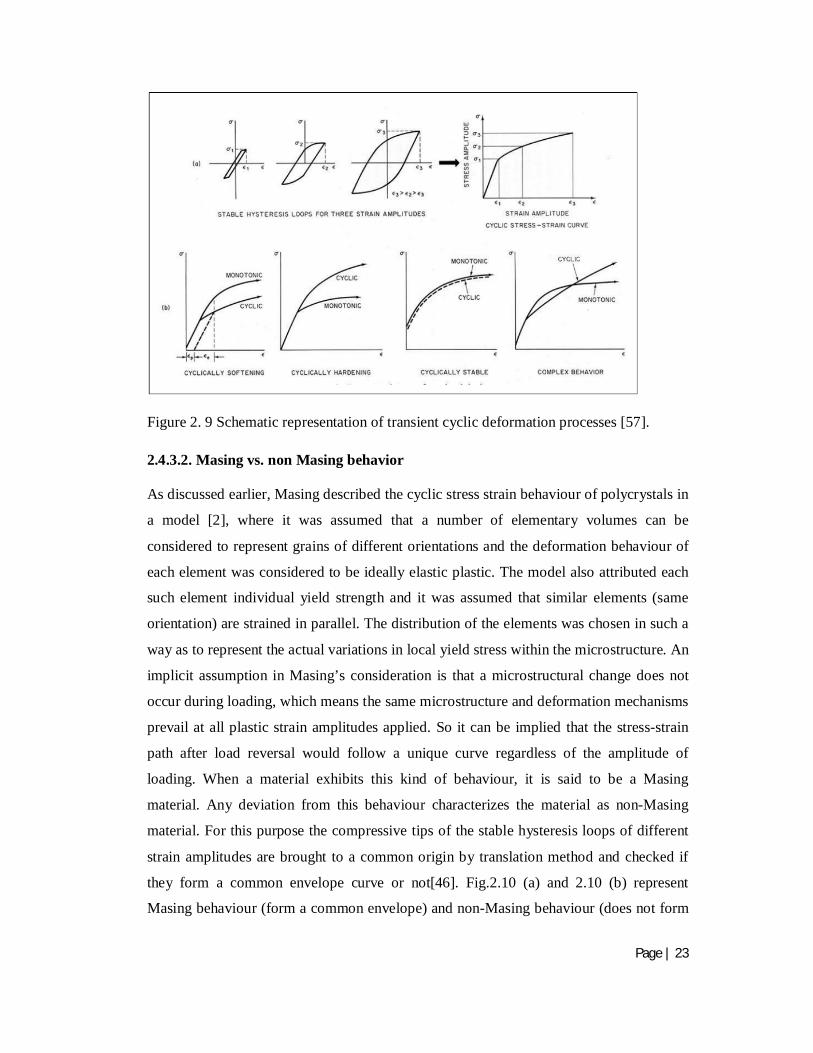
Figure 2. 9 Schematic representation of transient cyclic deformation processes. ......................... 23

Figure 2. 10 Schematic representation of (a) Masing behaviour (branco 2012) (b) non Masing behaviour (Paul 2011) ............................................................................................................... 24

Figure 2. 11 Typical master curve.............................................................................................. 25

Figure 2. 12 Plastic strain energy calculation (a) Masing material (right) (b) Non Masing material (left) .......................................................................................................................................... 26

Figure 2. 13 Schematic representation of S N curve ................................................................... 27

Figure 2. 14 Schematic representation of Coffin Mansion plot. .................................................. 28

Figure 2. 15 Total strain energy approach .................................................................................. 30

Figure 3. 1 Schematic representation of welded block ................................................................ 33

Figure 3. 2 Orientation and specimen preparation plan through pipe (a) Side view (b) Top view 35

Figure 3. 3 Tensile subsize weld specimen. All dimensions are in ‘mm’ ................................... 35

Figure 3. 4 Schematic diagram depicting flat sub size room temperature fatigue specimen ......... 36

Figure 3. 5 Typical wave form used for low cycle fatigue test. ................................................... 36

Figure 3. 6 Typical hysteresis loops as generated during experiment .......................................... 37

VIII

Figure 4. 1 Weld zone microstructure in different orientation (a) RC, (b) LC, (c) LR ................. 40

Figure 4. 2 Engineering stress strain curve for weld SS 308 ....................................................... 41

Figure 4. 3 True stress strain curve for weld SS 308 .................................................................. 42

Figure 4. 4 Fractograph of post tensile weld SS 308 specimen ................................................... 42

Figure 4. 5 Schematic diagram depicting Bauschinger effect ..................................................... 43

Figure 4. 6 Bauchinger strain ..................................................................................................... 44

Figure 4. 7 Bauchinger stress ..................................................................................................... 44

Figure 4. 8 Cyclic hardening softening behaviour ...................................................................... 45

Figure 4. 9 Degree of Hardening ............................................................................................... 46

Figure 4. 10 Effect of loop shape parameter on fatigue life. ....................................................... 47

Figure 4. 11 Cyclic stability curve ............................................................................................. 48

Figure 4. 12 Coffin Mansion plot ............................................................................................... 48

Figure 4. 13 Variation of energy absorption with fatigue life ..................................................... 49

Figure 4. 14 Cyclic stress strain curve ....................................................................................... 50

Figure 4. 15 Comparison of cyclic and monotonic stress strain curve ......................................... 51

Figure 4. 16 Non Masing behaviour of material ......................................................................... 52

Figure 4. 17 (a) Master curve for weld SS 308 and (b) calculation of parameters from master curve ......................................................................................................................................... 53

Figure 4. 18 (a) Comparison of CPSE and EPSE (b) Comparison with respect to strain amplitude ................................................................................................................................................. 53

Figure 4. 19 Walker model for predicting life ............................................................................ 54

Figure 4. 20 SWT model for fatigue life prediction .................................................................... 55

Figure 4. 21 Fractographs of post fatigued fracture surfaces at various strain amplitudes............ 55

IX

List of Tables

Table2. 1 Typical nuclear materials in service (Miteva taylor 2006) ................................ 7

Table2. 2 Review of published literature correlating different microstructural properties with different welding parameters ................................................................................. 10

Table2. 3 Factors affecting fatigue life........................................................................... 16

Table 3. 1 Summary of low cycle fatigue tests ............................................................... 37

Table 4. 1 Chemical composition of the material………………………………………..39

Table 4. 2 Ferrite volume fraction in weld SS ............................................................... 40

Table 4. 3 Average hardness values in weld zone .......................................................... 41

Table 4. 4 Tensile properties of weld SS 308 ................................................................. 41

Table 4. 5 Stable loop for different strain amplitudes ..................................................... 47

Table 4. 6 Comparison of walker and SWT equivalent stress...........................................55

List of Symbols

E Modulus of elasticity

K Strain hardening coefficient

n Strain hardening exponent

K' Cyclic strain hardening coefficient

n' Cyclic strain hardening exponent

σf Fatigue strength coefficient

b Fatigue strength exponent

f Fatigue ductility coefficient

c Fatigue ductility exponent

Nf Number of cycles to failure

σm Mean stress

X

H Hardening factor

He Hardening factor for strain controlled experiment

HS Hardening factor for stress controlled experiment

List of abbreviations

AHWR Advanced heavy water reactors

AISI American Iron and Steel Institute

ASME American Society of Mechanical Engineers

ASS Austenitic stainless steel

ASTM American Society for Testing and Materials

BWR Boiling Water Reactor

CPSE- Calculated plastic strain energy

CSSC- Cyclic stress strain curve

DMW Dissimilar Metal Weld

EPSE- Experimentally determined plastic strain energy

HCF High cycle fatigue

LCF Low cycle fatigue

LSP Loop shape parameter

MHTP Main heat transport piping system

MSSC- Monotonic stress strain curve

PWR Pressurized Water reactor

SEM Scanning electron microscope

SS Stainless steel

TEM Transmission electron microscope

UTS Ultimate tensile strength

YS Yield strength

XI

ABSTRACT

Dissimilar metal welds (DMW) are widely employed to meet various fabrication

requirements in the integrated structures. In advanced heavy water reactors (AHWR),

main heat transport (MHT) piping system is made of austenitic stainless steels (SS) and

the later part of the piping is often made of carbon steels mainly to reduce the overall cost

of the structure. These two metals (austenitic and carbon steels) are joined by DMW

using SS 308 electrode. The operating temperature of this structure varies from 25-285

°C. This fluctuation in temperature causes thermally induced elastic-plastic strain

reversals.

In the present investigation an attempt has been made to study the low cycle fatigue

(LCF) behaviour of AISI 308 stainless steel weld metal. All LCF tests were conducted at

ambient condition following the ASTM standard E-606[1]. These tests were conducted at

strain amplitudes of 0.5%, 0.7%, 1.0%, 1.2% and 1.5% under fully reversed cycles

(R=-1).

Various approaches such as (i) strain, (ii) energy, (iii) cyclic stress-strain curve (CSSC)

and (iv) master curve have been employed in this investigation[2]. Walker and Smith

Watson Topper (SWT) life estimation models have also been attempted in the present

study[3]. The experimental results indicate pronounced Bauschinger effect, softening

during lower strain amplitudes and Non Masing behaviour. Comparison of cyclic stress-

strain curve (CSSC) and monotonic stress strain curve (MSSC) shows complex

hardening-softening behaviour. It is also known that plastic strain (Δεp) is the

predominant cause of energy dissipation during low cycle fatigue[4]. The plastic strain

energy calculated from the experimental data and estimated using constitutive equation

follows linear relationship with strain amplitude. This however remains constant when

plotted as a function of number of cycles to failure. The observations exhibit that Walker

and SWT fatigue life prediction models hold well in predicting fatigue life of the present

material.

Key words: Dissimilar metal weld, Plastic strain energy, Low cycle fatigue, Weld SS308, Cyclic stress strain curve

Page | 1

Chapter 1

1.0 Introduction 1.1 Introduction 1.2 Objectives of the present work 1.3 Scope of the work 1.4 Layout of the thesis

Page | 2

Chapter 1

Introduction

1.1 Introduction

Nuclear energy is a clean, safe, reliable and competitive source of energy and can satisfy

the needs of industrial civilization, aspirations of the developing nations and replace a

significant part of the fossil fuels responsible for greenhouse gases. At present, nuclear

power plants provide about 6% of the world's energy and only 1% of energy requirements

of this nation [5]. The various advantages of nuclear energy often overshadowed by

concerns related to design and safety of nuclear power plants. Therefore structural

integrity of the encompassing components especially containing complex designs and

joining processes are always a cause of concern for the designers. Dissimilar Metal

Welding (DMW) is widely used joining process in these reactors. In nuclear power plants

such welds are necessary for connecting austenitic stainless steel pipes to ferritic or plain

carbon steel components [6]. These are used in safety class systems of all Pressurized

Water Reactor (PWR) and Advanced Heavy Water Reactor (AHWR) plants [6].

Austenitic stainless steels are often employed in these conditions because of their good

high temperature mechanical properties whereas plain carbon steels are used mainly for

the purpose of cost reduction. Many structural components in nuclear power plants

experience cyclic plasticity due to thermal reversals during startup and shut down

operations. These welds are exposed to temperatures ranging from room temperature to as

high as 823 K and pressure up to 100 MPa. The weld zone of these structures are often

considered as the weakest link and cyclic deformation/ fracture behaviour of these

structures are influenced by their presence [7]. The importance of cyclic plastic

deformation and fracture has attracted extensive research in last two decades [8][9][10].

In their resent studies Pavethan et al. studied high cycle fatigue behaviour of medium

carbon and austenitic stainless steel welds and reported S-N curves of the materials [8].

Sivaprasad et al. investigated the low cycle fatigue and crack growth behaviour of

Page | 3

austenitic stainless steel and plain carbon steel weld and reported Coffin Mansion plot

and Paris law parameters for the materials [10]. However, energy based approach,

Masing/ non Masing behaviour, comparison of cyclic stress-strain curve (CSSC) and

monotonic stress strain curve (MSSC) for SS 308 weld metal are not available in

literature. The present investigation is dedicated to characterize the low cycle fatigue

behaviour of SS 308 weld metal and study its above mentioned behaviour.

1.2 Objective of the present work The main objective of the present investigation is to study and investigate the low

cycle fatigue characterization of AISI 308 weld metal.

1.3 Scope of the work

The major scope of the work can be broadly summarized as:

(I) To characterize microstructures and to determine mechanical properties of

the weld zone SS 308 stainless steel:

This part consists of (a) chemical composition analysis of the investigated material,

(b) microstructural examination and measurement of grain size, and (c) determination

of their hardness and tensile properties.

(II) To study the Low cycle fatigue behaviour of weld metal SS 308.

The major experiments to fulfil this objective are (a) strain controlled low cycle

fatigue experiments are conducted at various strain amplitudes (b) examination of the

micro mechanisms for fatigue damage using various fatigue analysis approaches.

(III) Fractographic examinations on fractured samples using scanning electron

microscopy.

Fractographic examination of fracture surface using SEM to study the various features

and to understand the mechanism involved in the fatigue failure of this metal.

Page | 4

1.4 Layout of the thesis

This thesis consists of five chapters. The requirement of related experiments along

with significance of the problem is described in Chapter-1. Literature background

related to fatigue behaviour of metal with special attention to DMW is presented in

Chapter-2. The present study has been inspired by the achievements of the previous

investigations and available gaps in this field. Details of various experimental

procedures related to chemical composition analysis, microstructure analysis,

hardness, tensile and low cycle fatigue are discussed in Chapter 3. The results

obtained from the investigation along with detailed discussion are discussed in

Chapter 4. Conclusions drawn from this work are summarized in Chapter-5 together

with some proposed future work related to this area. All references cited throughout

are compiled at the end of thesis in reference section.

Page | 5

Chapter 2

2.0 Literature review 2.1 Introduction 2.2 Nuclear reactor and piping materials 2.3 Dissimilar metal weld (DMW) 2.3.1. Types of DMW 2.3.2. Applications of DMW 2.3.3. Mechanisms of dissimilar metal joint failure 2.3.4. Precautions to minimize failure 2.4 Fatigue in metallic materials

2.4.1. Cyclic loading on materials 2.4.1.1. Fatigue failure mechanism 2.4.1.2. Types of cyclic loadings 2.4.1.3. Factors affecting fatigue life 2.4.2. Material response to cyclic deformation 2.4.2.1. Bauschinger effect (Stress strain anisotropy) 2.4.2.2. Hardening softening behaviour 2.4.2.3. Mean stress relaxation 2.4.2.4. Ratcheting 2.4.3. Loop Analysis 2.4.3.1. Cyclic stress strain curve (CSSC) 2.4.3.2. Masing / non Masing behaviour 2.4.3.3. Master curve 2.4.3.4. Plastic strain energy 2.4.4. Different approaches for predicting fatigue life 2.4.4.1. Stress based approach 2.4.4.2. Strain based approach 2.4.4.3. Energy based approach 2.4.5 Fatigue life estimation models 2.4.5.1. Walker parameter 2.4.5.2. SWT lifing equation 2.5 Summary

Page | 6

Chapter 2

Literature review

2.1 Introduction It is by now well perceived that research related to low cycle fatigue behaviour of DMW

materials is of adequate academic as well as practical importance. Investigations related

to mechanical behaviour of DMW materials has been accelerated in the last decade of the

past century. This chapter deals with reported work on fatigue behaviour including low

cycle fatigue of various metals and dissimilar metal welds. However literature related to

fatigue behaviour of weldment is limited. It is therefore seemed prerequisite to do a

survey of work done so far and material systems studied under fatigue behaviour of

DMW. A brief review of earlier work is incorporated in different sections of this chapter

to enhance the basic understanding of the topic. Different materials in service of nuclear

and other pressure vessel piping’s are discussed in section 2.2. Brief introduction to

DMW, their applications, its failure mechanism and prevention are reported in section

2.3. Cyclic deformation behaviour of metallic materials, different approaches towards

them and various phenomena involved are discussed in section 2.4. A summary of the

topics discussed in this chapter is presented in section 2.5 along with the design of the

current research problem on the basis of previously reported literature.

2.2 Nuclear reactor and pressure vessel piping materials

The ever expanding demands of energy have increased our dependence on various

nuclear, thermal and other types of power generation systems. These advanced power

generation systems create more stringent service conditions (high temperature and

pressure) which triggers the quest for higher and more energy efficient material with

better thermal, mechanical and anti-corrosive properties. The vast fraternity of materials

is available for selection but economic constraint and fabricability issues put further

limitations on design engineers. Steel is widely used as piping material in various

Page | 7

pressure vessel systems due to its relative low cost and vast experience which has been

acquired from its extensive use over time. For example, stainless steels like austenitic,

ferritic, martensitic and duplex; special structural steels like SA 508, SA533 steels;

different micro alloyed steels like Mn-Mo-Ni alloy steel, Mn-V-Ni alloy steel, Cr-Mo

alloy steel etc. are in use as per the ASME Pressure Vessel and Boiler Code[11].

Traditionally, austenitic stainless steels have been used in the higher temperature regions

of piping systems due to their good creep strength, thermal expansion coefficients, ease of

fabrication and their excellent oxidation and corrosion resistance due to higher chromium

contents which stabilize the austenite phase field and also combine with oxygen to form a

protective oxide layer on the surface. Table 2.1 reports the typical materials (structural

and stainless steels grades) present in service,

Table2. 1 Typical nuclear materials in service [6]

Material Part used Operating conditions Standard SA 508 Cl. 2 Nozzle materials 350*C, 15 MPa ASME SA 508 Cl 3 Nozzle materials 285*C, 15 MPa ASME SS 304 Piping material 350*C, 15 MPa ASME SS 304 LN Piping material 350*C, 15 MPa ASME SS 316 Piping material 350*C, 15 MPa ASME SS 316 L Piping material 350*C, 15 MPa ASME SA 333 Piping material 350*C, 15 MPa ASME SS 309 Filler material 350*C, 15 MPa ASME SS 308 Filler material 350*C, 15 MPa ASME 2.3 Dissimilar metal weld Welding is a most common phenomenon for joining of metals. DMW is a kind of process

used to join different materials. This approach is used when transition in mechanical

properties or other performance related parameters are required. In general joining of

different materials is more difficult because it requires adequate knowledge of physical,

chemical, mechanical and other performance parameters of all the included materials.

Furthermore the choice of filler materials is more difficult due to its compatibility issues

with base materials. [6][12].

2.3.1 Types of DMW

Various types of DMW are described in this section.

1. Two different materials joined together directly.

Page | 8

2. Two materials joined after buttering one of these with a layer of suitable material.

3. Two materials are joined by placing a transition piece between them.

4. Cladding of two materials (One material is coated by another material for a particular property enhancement purpose).[12]

2.3.2 Applications of DMW

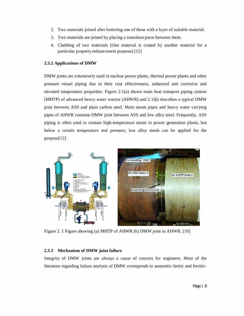
DMW joints are extensively used in nuclear power plants, thermal power plants and other

pressure vessel piping due to their cost effectiveness, enhanced anti corrosive and

elevated temperature properties. Figure 2.1(a) shows main heat transport piping system

(MHTP) of advanced heavy water reactor (AHWR) and 2.1(b) describes a typical DMW

joint between ASS and plain carbon steel. Main steam pipes and heavy water carrying

pipes of AHWR contains DMW joint between ASS and low alloy steel. Frequently, ASS

piping is often used to contain high-temperature steam in power generation plants, but

below a certain temperature and pressure, low alloy steels can be applied for the

purpose[12].

Figure 2. 1 Figure showing (a) MHTP of AHWR (b) DMW joint in AHWR. [10]

2.3.3 Mechanism of DMW joint failure

Integrity of DMW joints are always a cause of concern for engineers. Most of the

literature regarding failure analysis of DMW corresponds to austenitic-feritic and ferritic-

Page | 9

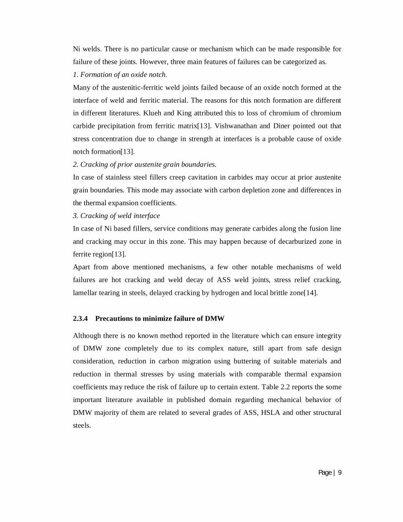
Ni welds. There is no particular cause or mechanism which can be made responsible for

failure of these joints. However, three main features of failures can be categorized as.

1. Formation of an oxide notch.

Many of the austenitic-ferritic weld joints failed because of an oxide notch formed at the

interface of weld and ferritic material. The reasons for this notch formation are different

in different literatures. Klueh and King attributed this to loss of chromium of chromium

carbide precipitation from ferritic matrix[13]. Vishwanathan and Diner pointed out that

stress concentration due to change in strength at interfaces is a probable cause of oxide

notch formation[13].

2. Cracking of prior austenite grain boundaries.

In case of stainless steel fillers creep cavitation in carbides may occur at prior austenite

grain boundaries. This mode may associate with carbon depletion zone and differences in

the thermal expansion coefficients.

3. Cracking of weld interface

In case of Ni based fillers, service conditions may generate carbides along the fusion line

and cracking may occur in this zone. This may happen because of decarburized zone in

ferrite region[13].

Apart from above mentioned mechanisms, a few other notable mechanisms of weld

failures are hot cracking and weld decay of ASS weld joints, stress relief cracking,

lamellar tearing in steels, delayed cracking by hydrogen and local brittle zone[14].

2.3.4 Precautions to minimize failure of DMW

Although there is no known method reported in the literature which can ensure integrity

of DMW zone completely due to its complex nature, still apart from safe design

consideration, reduction in carbon migration using buttering of suitable materials and

reduction in thermal stresses by using materials with comparable thermal expansion

coefficients may reduce the risk of failure up to certain extent. Table 2.2 reports the some

important literature available in published domain regarding mechanical behavior of

DMW majority of them are related to several grades of ASS, HSLA and other structural

steels.

Page | 10

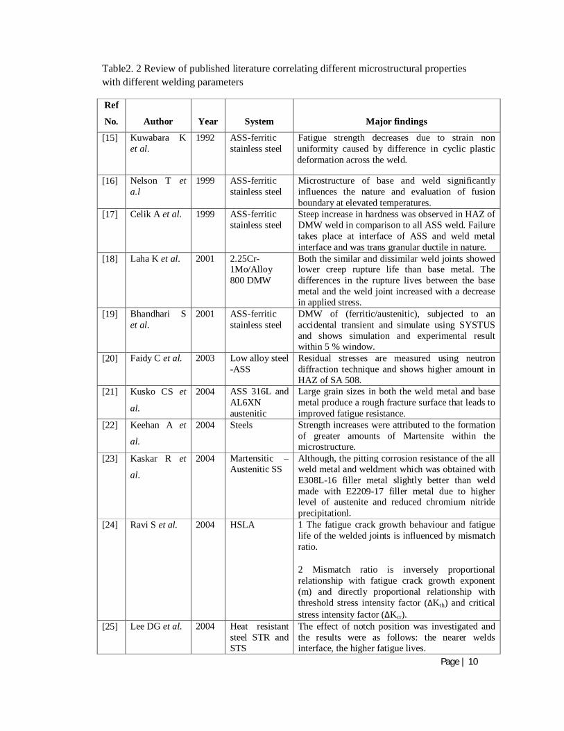
Table2. 2 Review of published literature correlating different microstructural properties with different welding parameters

Ref

No. Author Year System Major findings

[15] Kuwabara K et al.

1992 ASS-ferritic stainless steel

Fatigue strength decreases due to strain non uniformity caused by difference in cyclic plastic deformation across the weld.

[16] Nelson T et a.l


Microstructure of base and weld significantly influences the nature and evaluation of fusion boundary at elevated temperatures.

[17] Celik A et al. 1999 ASS-ferritic stainless steel

Steep increase in hardness was observed in HAZ of DMW weld in comparison to all ASS weld. Failure takes place at interface of ASS and weld metal interface and was trans granular ductile in nature.

[18] Laha K et al. 2001 2.25Cr-1Mo/Alloy 800 DMW

Both the similar and dissimilar weld joints showed lower creep rupture life than base metal. The differences in the rupture lives between the base metal and the weld joint increased with a decrease in applied stress.

[19] Bhandhari S et al.


DMW of (ferritic/austenitic), subjected to an accidental transient and simulate using SYSTUS and shows simulation and experimental result within 5 % window.

[20] Faidy C et al. 2003 Low alloy steel -ASS

Residual stresses are measured using neutron diffraction technique and shows higher amount in HAZ of SA 508.

[21] Kusko CS et

al.

2004 ASS 316L and AL6XN austenitic

Large grain sizes in both the weld metal and base metal produce a rough fracture surface that leads to improved fatigue resistance.

[22] Keehan A et

al.

2004 Steels Strength increases were attributed to the formation of greater amounts of Martensite within the microstructure.

[23] Kaskar R et

al.

2004 Martensitic –Austenitic SS

Although, the pitting corrosion resistance of the all weld metal and weldment which was obtained with E308L-16 filler metal slightly better than weld made with E2209-17 filler metal due to higher level of austenite and reduced chromium nitride precipitationl.

[24] Ravi S et al. 2004 HSLA 1 The fatigue crack growth behaviour and fatigue life of the welded joints is influenced by mismatch ratio.

2 Mismatch ratio is inversely proportional relationship with fatigue crack growth exponent (m) and directly proportional relationship with threshold stress intensity factor (ΔKth) and critical stress intensity factor (ΔKcr).

[25] Lee DG et al. 2004 Heat resistant steel STR and STS

The effect of notch position was investigated and the results were as follows: the nearer welds interface, the higher fatigue lives.

Page | 11

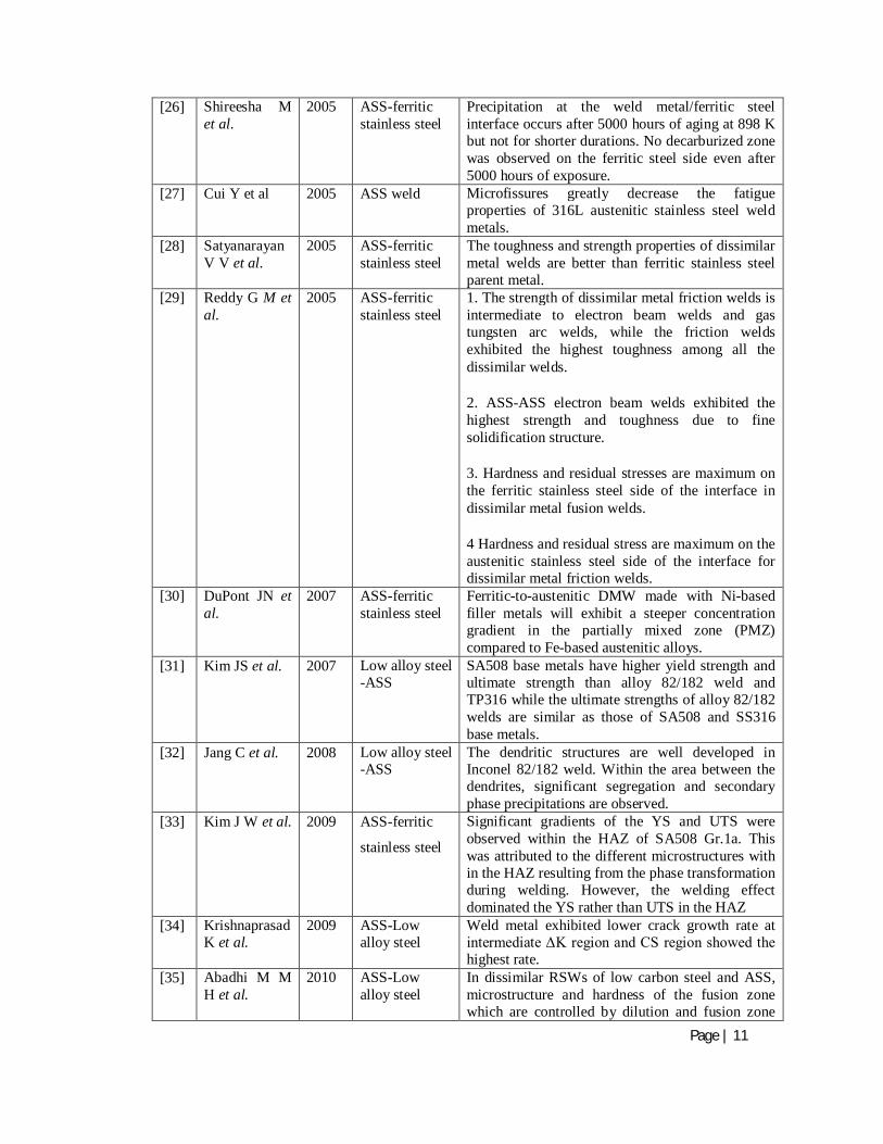
[26] Shireesha M et al.


Precipitation at the weld metal/ferritic steel interface occurs after 5000 hours of aging at 898 K but not for shorter durations. No decarburized zone was observed on the ferritic steel side even after 5000 hours of exposure.

[27] Cui Y et al 2005 ASS weld Microfissures greatly decrease the fatigue properties of 316L austenitic stainless steel weld metals.

[28] Satyanarayan V V et al.


The toughness and strength properties of dissimilar metal welds are better than ferritic stainless steel parent metal.

[29] Reddy G M et al.


1. The strength of dissimilar metal friction welds is intermediate to electron beam welds and gas tungsten arc welds, while the friction welds exhibited the highest toughness among all the dissimilar welds.

2. ASS-ASS electron beam welds exhibited the highest strength and toughness due to fine solidification structure.

3. Hardness and residual stresses are maximum on the ferritic stainless steel side of the interface in dissimilar metal fusion welds.

4 Hardness and residual stress are maximum on the austenitic stainless steel side of the interface for dissimilar metal friction welds.

[30] DuPont JN et al.


Ferritic-to-austenitic DMW made with Ni-based filler metals will exhibit a steeper concentration gradient in the partially mixed zone (PMZ) compared to Fe-based austenitic alloys.

[31] Kim JS et al. 2007 Low alloy steel -ASS

SA508 base metals have higher yield strength and ultimate strength than alloy 82/182 weld and TP316 while the ultimate strengths of alloy 82/182 welds are similar as those of SA508 and SS316 base metals.

[32] Jang C et al. 2008 Low alloy steel -ASS

The dendritic structures are well developed in Inconel 82/182 weld. Within the area between the dendrites, significant segregation and secondary phase precipitations are observed.

[33] Kim J W et al. 2009 ASS-ferritic

stainless steel

Significant gradients of the YS and UTS were observed within the HAZ of SA508 Gr.1a. This was attributed to the different microstructures with in the HAZ resulting from the phase transformation during welding. However, the welding effect dominated the YS rather than UTS in the HAZ

[34] Krishnaprasad K et al.

2009 ASS-Low alloy steel

Weld metal exhibited lower crack growth rate at intermediate ΔK region and CS region showed the highest rate.

[35] Abadhi M M H et al.

2010 ASS-Low alloy steel

In dissimilar RSWs of low carbon steel and ASS, microstructure and hardness of the fusion zone which are controlled by dilution and fusion zone

Page | 12

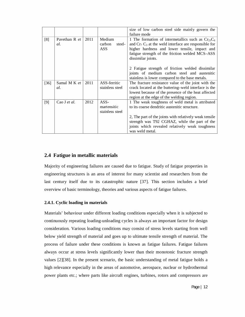
size of low carbon steel side mainly govern the failure mode

[8] Pavethan R et al.

2011 Medium carbon steel- ASS

1 The formation of intermetallics such as Cr23C6 and Cr7 C3 at the weld interface are responsible for higher hardness and lower tensile, impact and fatigue strength of the friction welded MCS–ASS dissimilar joints.

2 Fatigue strength of friction welded dissimilar joints of medium carbon steel and austenitic stainless is lower compared to the base metals.

[36] Samal M K et al.


The fracture resistance value of the joint with the crack located at the buttering–weld interface is the lowest because of the presence of the heat affected region at the edge of the welding region.

[9] Cao J et al. 2012 ASS-martensitic stainless steel

1 The weak toughness of weld metal is attributed to its coarse dendritic austenitic structure.

2, The part of the joints with relatively weak tensile strength was T92 CGHAZ, while the part of the joints which revealed relatively weak toughness was weld metal.

2.4 Fatigue in metallic materials

Majority of engineering failures are caused due to fatigue. Study of fatigue properties in

engineering structures is an area of interest for many scientist and researchers from the

last century itself due to its catastrophic nature [37]. This section includes a brief

overview of basic terminology, theories and various aspects of fatigue failures.

2.4.1. Cyclic loading in materials

Materials’ behaviour under different loading conditions especially when it is subjected to

continuously repeating loading-unloading cycles is always an important factor for design

consideration. Various loading conditions may consist of stress levels starting from well

below yield strength of material and goes up to ultimate tensile strength of material. The

process of failure under these conditions is known as fatigue failures. Fatigue failures

always occur at stress levels significantly lower than their monotonic fracture strength

values [2][38]. In the present scenario, the basic understanding of metal fatigue holds a

high relevance especially in the areas of automotive, aerospace, nuclear or hydrothermal

power plants etc.; where parts like aircraft engines, turbines, rotors and compressors are

Page | 13

continuously subjected to vibration and fluctuating stresses. Fatigue failure may be

catastrophic in nature but process of failure is progressive and consists of several stages.

These stages and underlying failure mechanisms along with nomenclature and types of

cyclic loading are discussed in section 2.4.1.1. Section 2.4.1.2 includes a brief discussion

over major classification of fatigue on the basis of fatigue life of material like low cycle

fatigue, high cycle fatigue and ratcheting.

Apart from repeated loads several other factors like temperature, environmental factors,

geometry, sudden overloading, microstructure of material, residual stresses, and stress

concentration may significantly influence the life of the material. These factors are

discussed in more detail in section 2.4.1.3.

2.4.1.1. Mechanism of fatigue failure

The fatigue crack initiation process generally starts from free surface due to higher stresses

and probable presence of defects like scratches, corrosive pits etc. It is also observed that

fatigue cracks initiate even at highly polished defect free surfaces. The process of fatigue

failure initiates with the formation of mature cracks that may grow during component’s

service life. Various microscopic changes that lead to change in crystalline structure of metals

may occur under these conditions. These small scale changes increase the formation of small

cracks. These small cracks further develop into larger cracks which grow continuously till the

stresses become unsustainable and then catastrophic failure occurs. The process of fatigue

failure can therefore be sub divided into three major stages (a) initiation of numerous small

fatigue cracks, (b) growth of smaller number of small cracks into the larger ones and (c) final

failure which is caused by a single through crack which propagates though the complete cross

section of the components[37].

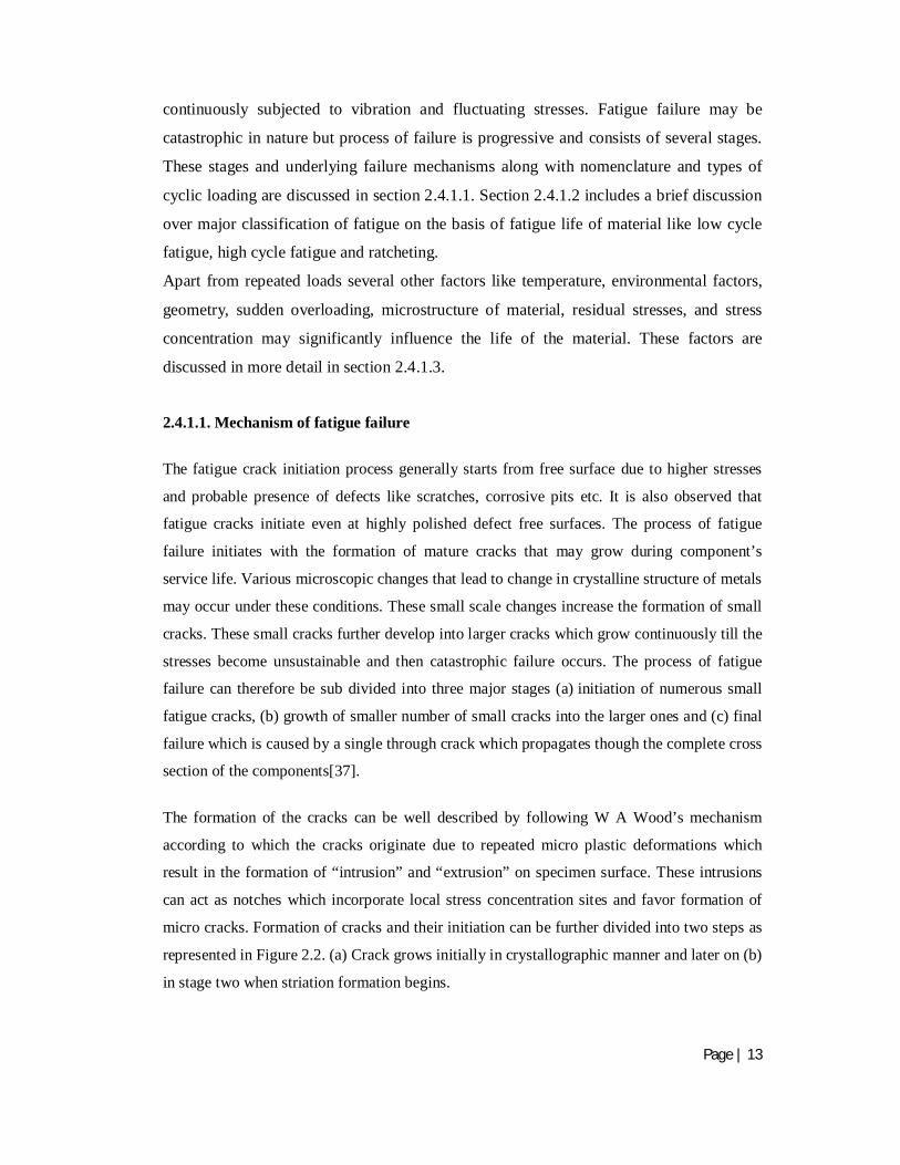
The formation of the cracks can be well described by following W A Wood’s mechanism

according to which the cracks originate due to repeated micro plastic deformations which

result in the formation of “intrusion” and “extrusion” on specimen surface. These intrusions

can act as notches which incorporate local stress concentration sites and favor formation of

micro cracks. Formation of cracks and their initiation can be further divided into two steps as

represented in Figure 2.2. (a) Crack grows initially in crystallographic manner and later on (b)

in stage two when striation formation begins.

Page | 14

Figure 2. 2 Schematic representation of striation formation during fatigue crack growth [2,38].

Propagation of fatigue crack occurs through repeated crack tip blunting and sharpening

effects. After a prolonged period of time this micro-plastic deformation mechanisms

operating at the crack tip may cause characteristic markings which are called “beach

markings” or “clamshell markings”. These markings are macroscopic in nature and can be

visualized through a naked eye. On the other hand, there are extremely fine parallel markings,

at intervals of the order of 0.1 μm called “striations”, which represent the crack growth or

crack front due to each individual loading cycles and can see at higher magnifications using

electron microscopes.

It has been observed that limited number of alternative slip planes occurred during crack tip

plasticity. The resultant movement of dislocations is also limited to certain number of planes.

Increasing number of dislocations near the crack tip cause pile up and result in localized work

hardening. Resultant work hardening eases crack growth on slip plane by embritlling the

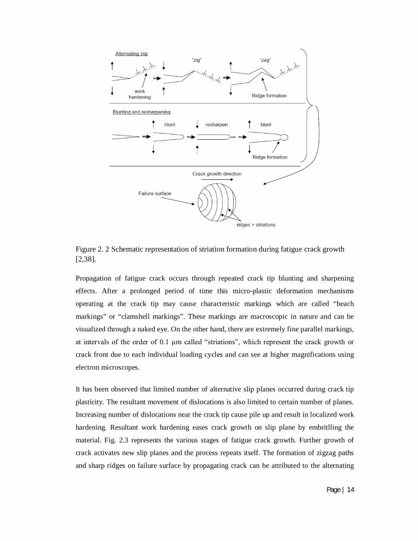
material. Fig. 2.3 represents the various stages of fatigue crack growth. Further growth of

crack activates new slip planes and the process repeats itself. The formation of zigzag paths

and sharp ridges on failure surface by propagating crack can be attributed to the alternating

Page | 15

slip planes. Upon loading, the initially sharp crack will blunt due to plastic deformation and

thus the lengths of small cracks increase due to blunting.

Figure 2. 3 Schematic representations of the various stages of fatigue crack growth [2]

When the crack is unloaded, the elastic stress field around the plastically relaxed crack tip

will cause the crack to resharpen. The further reloading of the crack, blunting is again,

leave a ripple on the surface. Further on, in Stage III, static fracture modes are

superimposed on the growth mechanism, till finally it fails catastrophically by shear at an

angle to the direction of growth.

Different nomenclature to describe test parameters

Different nomenclature is there in fatigue literature which can be enlisted as follows:

2.4.1.2. Types of cyclic loading

Page | 16

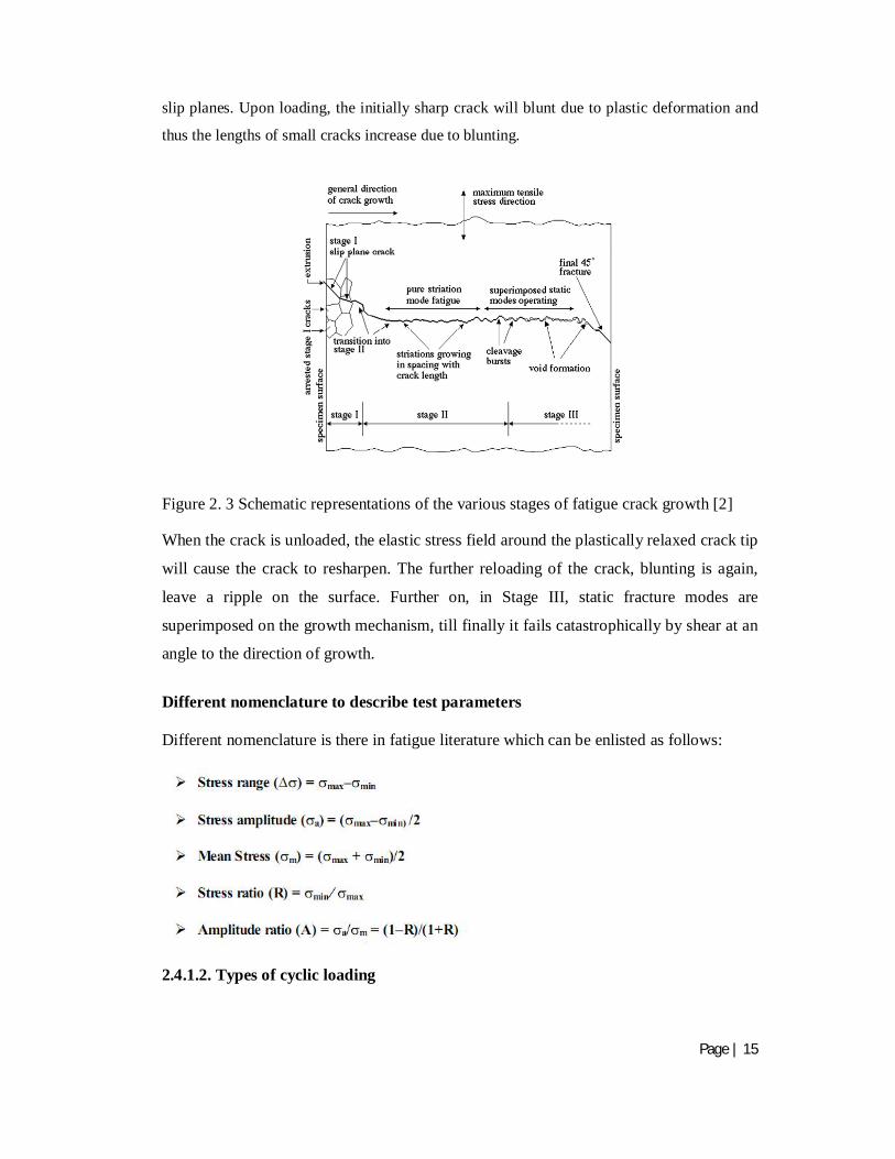
As can be seen from Fig 2.4, cyclic loading may be of different types. These are: [Dieter

1998] completely reversed cycle: In this type of cyclic loading, maximum and minimum

stresses are equal. It can also be referred as symmetric loading (σm = 0). Tensile stress is

considered positive and compressive stress is negative (Fig 2.4(a)).

Figure 2. 4 (a) completely reversed stress cycle (b) asymmetric stress cycle (c) Random stress cycle.[37]

Asymmetric loading: repeated stress cycle in which the maximum stress σmax and σmin are

not equal. Both are in tension, but sometimes it may be tension and compression both.

This is known as asymmetric loading (σm ≠ 0, Fig 2.4(b)). Random stress cycle: this type

of stress cycle generated in a part such as an aircraft wing which is subjected to periodic

unpredictable load due to gusts (Fig 2.4(c))[37].

2.4.1.3. Factors affecting fatigue life

Various parameters which play significant role in materials’ fatigue life are enlisted in

Table 2.3

Table2. 3 Factors affecting fatigue life

S.No. Parameter Role and Key Features

1 Microstructure In general at ambient temperature, grain size is inversely proportional

to fatigue life. Precipitate, grain boundaries, dislocation substructure

and density along with phase transformation also influences fatigue

Page | 17

life.

2 Processing type Rolling, forging extrusion etc. produces directional properties. Fatigue

life increases in longitudinal direction and decreases in transverse

direction. Other processes like Heat treatment, case hardening induces

residual stresses. Compressive residual stresses increases while tensile

residual stresses decreases fatigue life.

3 Type of

loading

Multiaxial loading reduces fatigue life more rapidly than uniaxial

loading except pure torsional case.

Alternating stress/strain has inverse relation with fatigue life.

4 Environmental

condition

Corrosive atmosphere can have a detrimental effect on fatigue life.

5 Geometrical

factors

Rough surfaces, notches, scratches, holes, joints decreases fatigue life

by increases stress concentration.

6 Temperature High temperatures T>0.5Tm fatigue life of material decreases. Grain

boundary triple points increases resulting high stress concentration

with increasing no. of grain boundary voids and wedge cracks.

2.4.2. Materials response to cyclic deformation

Any material when subjected to cyclic loading it’s deformation behaviour varies

according to the various applied stress/strain parameters which are described in

subsequent sections.

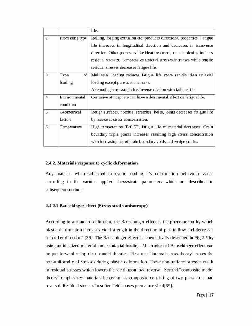
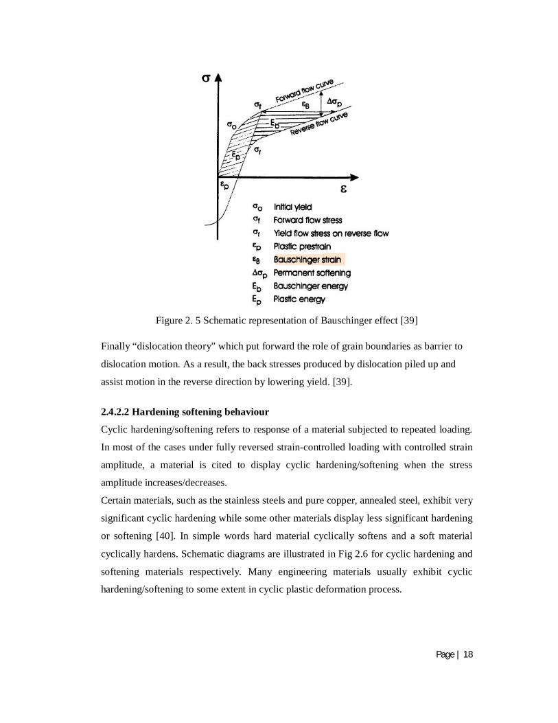
2.4.2.1 Bauschinger effect (Stress strain anisotropy)

According to a standard definition, the Bauschinger effect is the phenomenon by which

plastic deformation increases yield strength in the direction of plastic flow and decreases

it in other direction” [39]. The Bauschinger effect is schematically described in Fig 2.5 by

using an idealized material under uniaxial loading. Mechanism of Bauschinger effect can

be put forward using three model theories. First one “internal stress theory” states the

non-uniformity of stresses during plastic deformation. These non-uniform stresses result

in residual stresses which lowers the yield upon load reversal. Second “composite model

theory” emphasizes materials behaviour as composite consisting of two phases on load

reversal. Residual stresses in softer field causes premature yield[39].

Page | 18

Figure 2. 5 Schematic representation of Bauschinger effect [39]

Finally “dislocation theory” which put forward the role of grain boundaries as barrier to

dislocation motion. As a result, the back stresses produced by dislocation piled up and

assist motion in the reverse direction by lowering yield. [39].

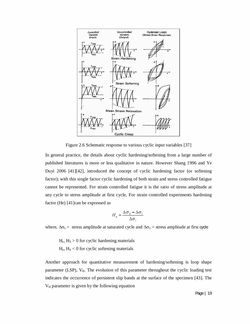
2.4.2.2 Hardening softening behaviour

Cyclic hardening/softening refers to response of a material subjected to repeated loading.

In most of the cases under fully reversed strain-controlled loading with controlled strain

amplitude, a material is cited to display cyclic hardening/softening when the stress

amplitude increases/decreases.

Certain materials, such as the stainless steels and pure copper, annealed steel, exhibit very

significant cyclic hardening while some other materials display less significant hardening

or softening [40]. In simple words hard material cyclically softens and a soft material

cyclically hardens. Schematic diagrams are illustrated in Fig 2.6 for cyclic hardening and

softening materials respectively. Many engineering materials usually exhibit cyclic

hardening/softening to some extent in cyclic plastic deformation process.

Page | 19

Figure 2.6 Schematic response to various cyclic input variables [37]

In general practice, the details about cyclic hardening/softening from a large number of

published literatures is more or less qualitative in nature. However Shang 1996 and Ye

Duyi 2006 [41][42], introduced the concept of cyclic hardening factor (or softening

factor); with this single factor cyclic hardening of both strain and stress controlled fatigue

cannot be represented. For strain controlled fatigue it is the ratio of stress amplitude at

any cycle to stress amplitude at first cycle, For strain controlled experiments hardening

factor (He) [41]can be expressed as

wheres = stress amplitude at saturated cycle and 1 = stress amplitude at first cycle

He, HS > 0 for cyclic hardening materials

He, HS < 0 for cyclic softening materials

Another approach for quantitative measurement of hardening/softening is loop shape

parameter (LSP), VH. The evolution of this parameter throughout the cyclic loading test

indicates the occurrence of persistent slip bands at the surface of the specimen [43]. The

VH parameter is given by the following equation

Page | 20

Where, W is the hysteresis loop area, εap is the plastic strain amplitude and σa is the stress

amplitude. During initial cyclic hardening and the development of the vein dislocation

structure, VH decreases. However, localization of plastic strain in persistent slip bands

(PSB’s) is accompanied by a significant increase in VH. This increase is especially

pronounced in single crystals, though it has also been observed in polycrystals [44]. After

the stress amplitude of the specimen cyclically saturates, VH either reaches a plateau or

decreases slightly.

2.4.2.3. Mean stress relaxation

Relaxation of mean stress happens when we do an unsymmetrical strain experiment, as

shown in Fig 2.6. For unsymmetrical strain experiment, a mean strain is introduced. Mean

strain cause mean stress. So at the initial cycle a mean stress is introduced during

unsymmetrical strain experiment. But as the cycling proceeds mean stress will relax and

tends to zero.

2.4.2.4. Ratcheting

Ratcheting is the event of progressive accumulation of permanent deformation when any

component is subjected to cyclic loads in the elastic plastic strain range under stress

controlled fatigue with non-zero mean stresses. Due to accumulation of plastic strain

material will finally lead to a shakedown, or a constant rate of ratcheting or very large

ratcheting strains ultimate to failure of the material [45]. Ratcheting is important in

designing and life evaluation of the structural components endured in cyclic loading.

Ratcheting strain is a secondary strain produced under asymmetrical cyclic stressing, and

has a great dependence on loading conditions and loading history

2.4.3 Loop analysis

2.4.3.1 Cyclic stress strain curve (CSSC)

As is shown in Fig. 2.7, the stress range, and the strain range

can be analogously be represented as. . The corresponding

amplitudes of stress and strain are half the ranges. The plastic strain range Δεpl is equal to

Page | 21

the distance between the points of intersection of the hysteresis loop and the strain axis, as

is shown in Fig. 2.8. Depending on the material, a more-or-less pronounced back

deformation may occur during unloading, which gives rise to a difference between Δεpl

and . This difference sometimes attributed to a “reversible plastic strain,”

an expression that itself seems contradictory. When constructing a strain-time history

from stress-time data hysteresis loop have to be constructed using the cyclic stress-

strain curve (CSSC). One key step is to determine when the line begins to bend as we

move from tension to compression and vice versa. This is handled by using Masing’s

hypothesis, which assumes that the line describing a stress-strain hysteresis loop is

geometrically similar to the CSSC but numerically twice its size[2]. Consequently, the

equation of the curve can be directly derived from the equation of CSSC. In order to

distinguish the parameters representing monotonic and cyclic ones, a prime symbol is

used for cyclic parameters. Corresponding to any point () on CSSC, we have,

Where, K′ is called the cyclic strength coefficient and n′ is called the cyclic strain

hardening exponent. From Masing’s hypothesis, the same point can be located on the

hysteresis loop curve and it will have coordinates (Δ,Δε) where:

Substituting into the equation for CSSC, we have

Which in general case reduces to

Thus we can establish the relationship between the cyclic stress-strain curve and

hysteresis loop shape. Proceeding on the similar grounds, we have

Page | 22

The cyclic stress-strain curve reflects the resistance of a material to cyclic deformation

and can be different from monotonic stress-strain curve.

Transient cyclic deformation behavior such as cyclic hardening or cyclic softening refers

to a continuous change in the cyclic strength that may occur throughout a test or at least

in the first stage of cyclic deformation. Schematic examples of cyclic hardening and

cyclic softening in are shown in Fig. 2.9 show the stress change and hysteresis loop

shape. Cyclic hardening leads to an increase in the stress amplitude, and consequently the

hysteresis loop becomes larger. Cyclic softening has the opposite effect a decrease of

and a reduction of the size of the hysteresis loop. The type of transient behavior is

mainly determined by the pretreatment of the material tested. It is plausible that, for

instance, heavy cold working prior to cyclic loading could cause subsequent cyclic

softening, whereas a recrystallization treatment could give rise to cyclic hardening.

Furthermore, deformation induced micro-structural changes may also be the reason for

transient deformation behavior.[37]

Figure 2. 8 Comparison of CSSC and MSSC curve illustrating cyclic hardening and cyclic softening respectively [57].

Figure 2. 7 Primary quantities of a hysteresis loop. [2]

Page | 23

Figure 2. 9 Schematic representation of transient cyclic deformation processes [57].

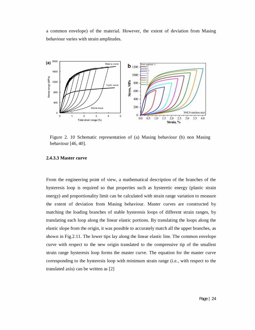
2.4.3.2. Masing vs. non Masing behavior

As discussed earlier, Masing described the cyclic stress strain behaviour of polycrystals in

a model [2], where it was assumed that a number of elementary volumes can be

considered to represent grains of different orientations and the deformation behaviour of

each element was considered to be ideally elastic plastic. The model also attributed each

such element individual yield strength and it was assumed that similar elements (same

orientation) are strained in parallel. The distribution of the elements was chosen in such a

way as to represent the actual variations in local yield stress within the microstructure. An

implicit assumption in Masing’s consideration is that a microstructural change does not

occur during loading, which means the same microstructure and deformation mechanisms

prevail at all plastic strain amplitudes applied. So it can be implied that the stress-strain

path after load reversal would follow a unique curve regardless of the amplitude of

loading. When a material exhibits this kind of behaviour, it is said to be a Masing

material. Any deviation from this behaviour characterizes the material as non-Masing

material. For this purpose the compressive tips of the stable hysteresis loops of different

strain amplitudes are brought to a common origin by translation method and checked if

they form a common envelope curve or not[46]. Fig.2.10 (a) and 2.10 (b) represent

Masing behaviour (form a common envelope) and non-Masing behaviour (does not form

Page | 24

a common envelope) of the material. However, the extent of deviation from Masing

behaviour varies with strain amplitudes.

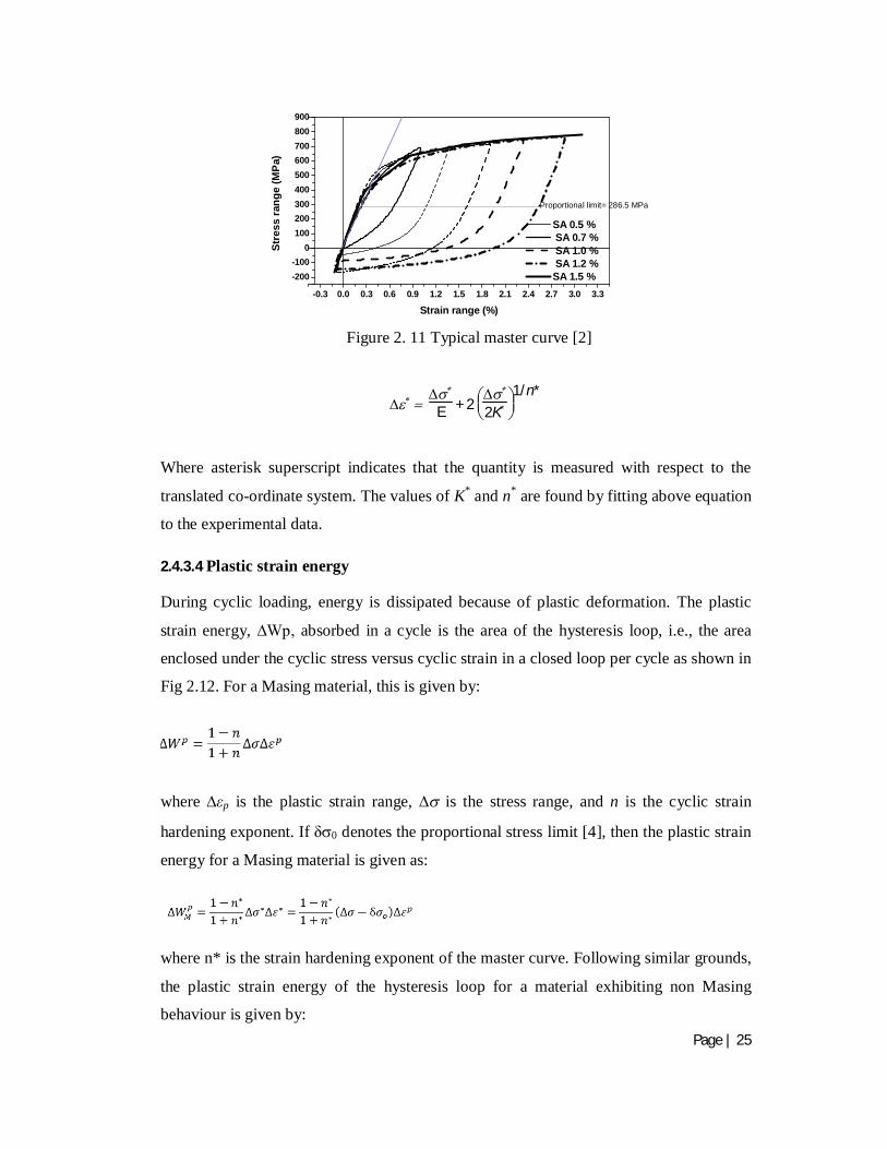
2.4.3.3 Master curve

From the engineering point of view, a mathematical description of the branches of the

hysteresis loop is required so that properties such as hysteretic energy (plastic strain

energy) and proportionality limit can be calculated with strain range variation to measure

the extent of deviation from Masing behaviour. Master curves are constructed by

matching the loading branches of stable hysteresis loops of different strain ranges, by

translating each loop along the linear elastic portions. By translating the loops along the

elastic slope from the origin, it was possible to accurately match all the upper branches, as

shown in Fig.2.11. The lower tips lay along the linear elastic line. The common envelope

curve with respect to the new origin translated to the compressive tip of the smallest

strain range hysteresis loop forms the master curve. The equation for the master curve

corresponding to the hysteresis loop with minimum strain range (i.e., with respect to the

translated axis) can be written as [2]

Figure 2. 10 Schematic representation of (a) Masing behaviour (b) non Masing behaviour [46, 40].

Page | 25

E + 2

2K1/n*

Where asterisk superscript indicates that the quantity is measured with respect to the

translated co-ordinate system. The values of K* and n* are found by fitting above equation

to the experimental data.

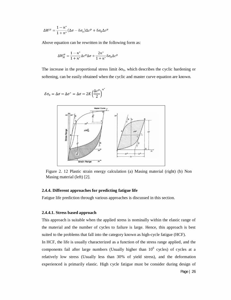
2.4.3.4 Plastic strain energy

During cyclic loading, energy is dissipated because of plastic deformation. The plastic

strain energy, ∆Wp, absorbed in a cycle is the area of the hysteresis loop, i.e., the area

enclosed under the cyclic stress versus cyclic strain in a closed loop per cycle as shown in

Fig 2.12. For a Masing material, this is given by:

where ∆εp is the plastic strain range, ∆ is the stress range, and n is the cyclic strain

hardening exponent. If δ0 denotes the proportional stress limit [4], then the plastic strain

energy for a Masing material is given as:

where n* is the strain hardening exponent of the master curve. Following similar grounds,

the plastic strain energy of the hysteresis loop for a material exhibiting non Masing

behaviour is given by:

-0.3 0.0 0.3 0.6 0.9 1.2 1.5 1.8 2.1 2.4 2.7 3.0 3.3

-200-100

0100200300400500600700800900

Stre

ss ra

nge

(MPa

)

Strain range (%)

SA 0.5 % SA 0.7 % SA 1.0 % SA 1.2 % SA 1.5 %

Proportional limit= 286.5 MPa

Figure 2. 11 Typical master curve [2]

Page | 26

Above equation can be rewritten in the following form as:

The increase in the proportional stress limit δ0, which describes the cyclic hardening or

softening, can be easily obtained when the cyclic and master curve equation are known.

2.4.4. Different approaches for predicting fatigue life

Fatigue life prediction through various approaches is discussed in this section.

2.4.4.1. Stress based approach

This approach is suitable when the applied stress is nominally within the elastic range of

the material and the number of cycles to failure is large. Hence, this approach is best

suited to the problems that fall into the category known as high-cycle fatigue (HCF).

In HCF, the life is usually characterized as a function of the stress range applied, and the

components fail after large numbers (Usually higher than 106 cycles) of cycles at a

relatively low stress (Usually less than 30% of yield stress), and the deformation

experienced is primarily elastic. High cycle fatigue must be consider during design of

Figure 2. 12 Plastic strain energy calculation (a) Masing material (right) (b) Non Masing material (left) [2].

Page | 27

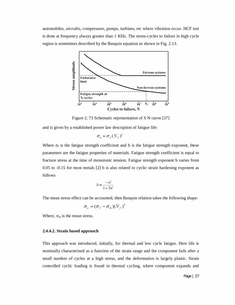
automobiles, aircrafts, compressors, pumps, turbines, etc where vibration occur. HCF test

is done at frequency always greater than 1 KHz. The stress-cycles to failure in high cycle

region is sometimes described by the Basquin equation as shown in Fig. 2.13.

Figure 2. 73 Schematic representation of S N curve [37] and is given by a established power law description of fatigue life:

Where σf is the fatigue strength coefficient and b is the fatigue strength exponent, these

parameters are the fatigue properties of materials. Fatigue strength coefficient is equal to

fracture stress at the time of monotonic tension. Fatigue strength exponent b varies from

0.05 to -0.15 for most metals [2] b is also related to cyclic strain hardening exponent as

follows

The mean stress effect can be accounted, then Basquin relation takes the following shape:

Where, σm is the mean stress.

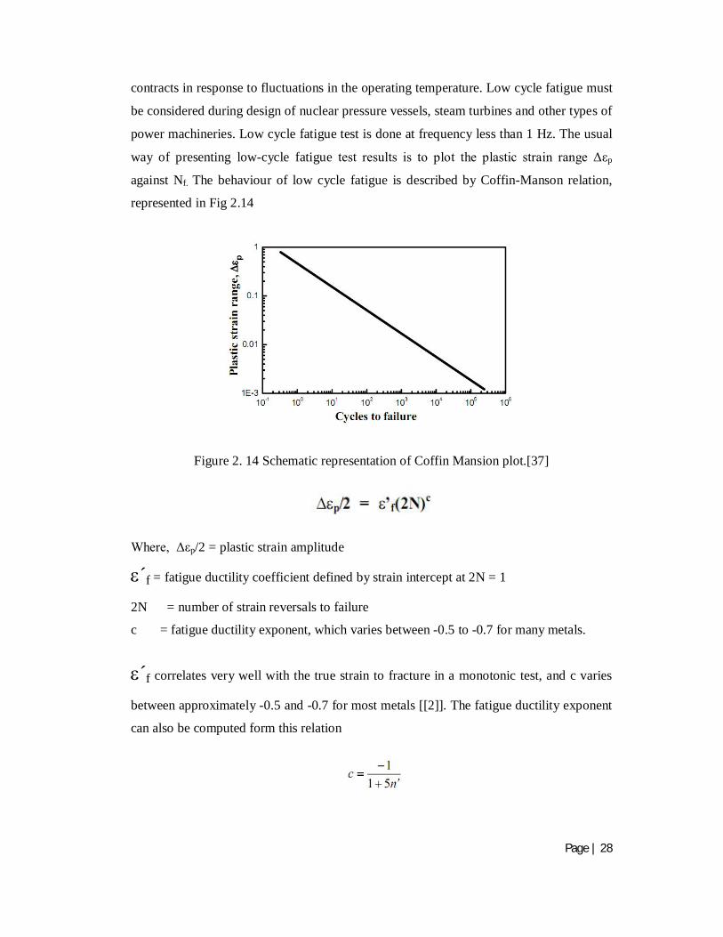
2.4.4.2. Strain based approach

This approach was introduced, initially, for thermal and low cycle fatigue. Here life is

nominally characterized as a function of the strain range and the component fails after a

small number of cycles at a high stress, and the deformation is largely plastic. Strain

controlled cyclic loading is found in thermal cycling, where component expands and

Page | 28

contracts in response to fluctuations in the operating temperature. Low cycle fatigue must

be considered during design of nuclear pressure vessels, steam turbines and other types of

power machineries. Low cycle fatigue test is done at frequency less than 1 Hz. The usual

way of presenting low-cycle fatigue test results is to plot the plastic strain range Δεp

against Nf. The behaviour of low cycle fatigue is described by Coffin-Manson relation,

represented in Fig 2.14

Figure 2. 14 Schematic representation of Coffin Mansion plot.[37]

Where, Δεp/2 = plastic strain amplitude

´f = fatigue ductility coefficient defined by strain intercept at 2N = 1

2N = number of strain reversals to failure

c = fatigue ductility exponent, which varies between -0.5 to -0.7 for many metals.

´f correlates very well with the true strain to fracture in a monotonic test, and c varies

between approximately -0.5 and -0.7 for most metals [[2]]. The fatigue ductility exponent

can also be computed form this relation

Page | 29

2.4.4.3. Energy based approach

On the microscopic level, the irreversible nature of micro plastic deformation caused by

each cycle of loading is associated with the dissipation of strain energy density. The

dissipation strain energy density per cycle may be regarded as a contributor to the fatigue

damage process per cycle. This approach can be broadly classified into two sub-

categories as follows:1. Hysterisis based approach 2. Total energy approach

Hysterisis based approach: discussed earlier

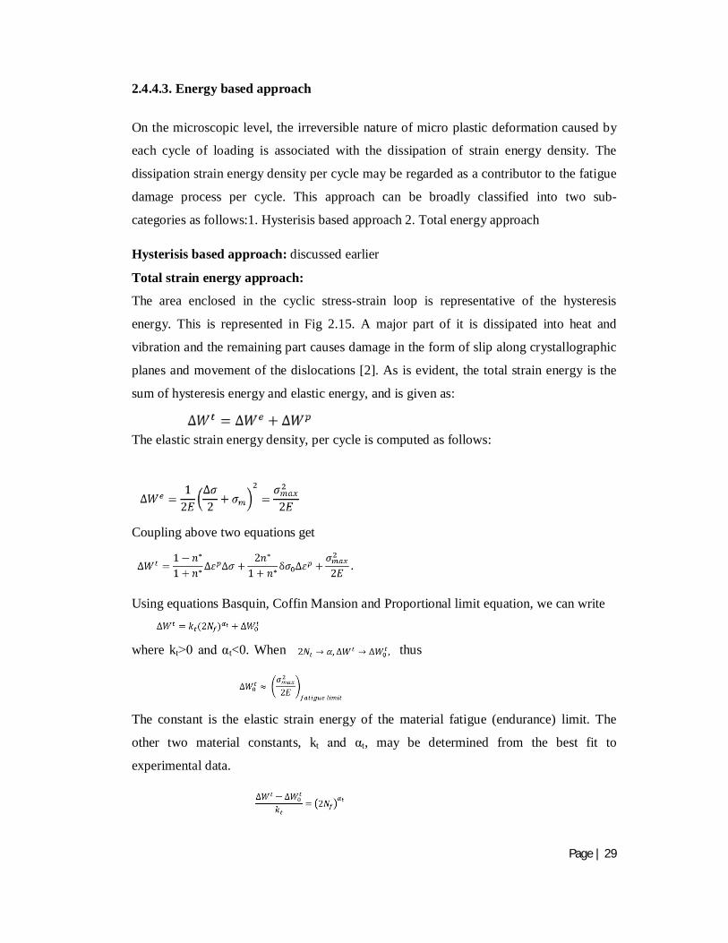
Total strain energy approach:

The area enclosed in the cyclic stress-strain loop is representative of the hysteresis

energy. This is represented in Fig 2.15. A major part of it is dissipated into heat and

vibration and the remaining part causes damage in the form of slip along crystallographic

planes and movement of the dislocations [2]. As is evident, the total strain energy is the

sum of hysteresis energy and elastic energy, and is given as:

The elastic strain energy density, per cycle is computed as follows:

Coupling above two equations get

Using equations Basquin, Coffin Mansion and Proportional limit equation, we can write

where kt>0 and αt<0. When thus

The constant is the elastic strain energy of the material fatigue (endurance) limit. The

other two material constants, kt and αt, may be determined from the best fit to

experimental data.

Page | 30

2.4.5 Fatigue life estimation models

In the design and development of engineering components fatigue life predictions takes

important role. Various methods that can be used for predicting fatigue life are .Basquin,

Coffin Mansion, Smith Watson Topper (SWT) and Walker equation etc. Basquin’s

equation and Coffin Mansion equation are already discussed in earlier sections so

remaining methods (SWT and Walker) are discussed in this section.

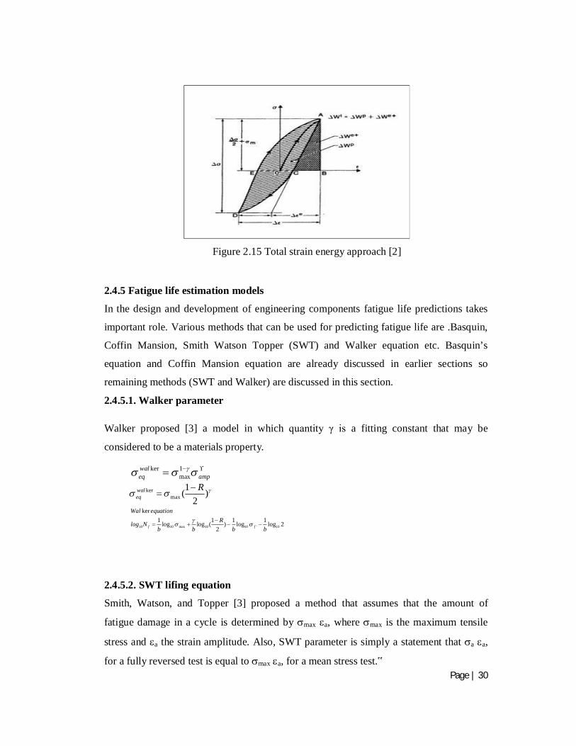
2.4.5.1. Walker parameter Walker proposed [3] a model in which quantity γ is a fitting constant that may be

considered to be a materials property.

2.4.5.2. SWT lifing equation

Smith, Watson, and Topper [3] proposed a method that assumes that the amount of

fatigue damage in a cycle is determined by max a, where max is the maximum tensile

stress and a the strain amplitude. Also, SWT parameter is simply a statement that a a,

for a fully reversed test is equal to max a, for a mean stress test.‟

10 10 max 10 10 ' 10

ker1 1 1 1log log ( ) log log 2

2f f

Wal equationRlog N

b b b b

kermax

1( )2

waleq

R

ker 1max

waleq amp

Figure 2.15 Total strain energy approach [2]

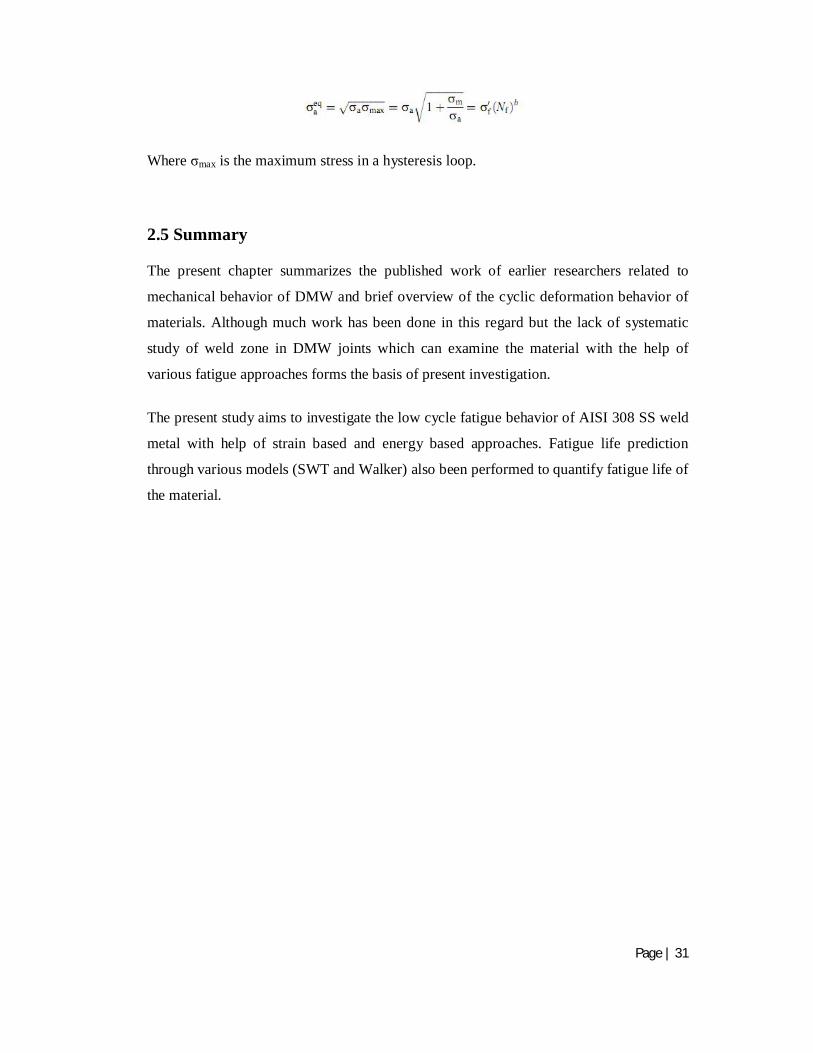
Page | 31

Where σmax is the maximum stress in a hysteresis loop.

2.5 Summary

The present chapter summarizes the published work of earlier researchers related to

mechanical behavior of DMW and brief overview of the cyclic deformation behavior of

materials. Although much work has been done in this regard but the lack of systematic

study of weld zone in DMW joints which can examine the material with the help of

various fatigue approaches forms the basis of present investigation.

The present study aims to investigate the low cycle fatigue behavior of AISI 308 SS weld

metal with help of strain based and energy based approaches. Fatigue life prediction

through various models (SWT and Walker) also been performed to quantify fatigue life of

the material.

Page | 32

Chapter 3

3.0 Materials and methods 3.1 Introduction 3.2 Experimentation 3.2.1 Material 3.2.2 Chemical composition 3.2.3 Optical microscopy 3.2.4 Hardness measurement 3.2.5 Tensile test 3.2.6 Low cycle fatigue 3.2.7 Scanning electron microscopy

Page | 33

Chapter 3

Materials and Methods

3.1 Introduction

A brief introduction to the weld metal (material under investigation), the dimensional

details of the low cycle fatigue specimen and basic material characterizations are

described in this chapter. The study of low cycle fatigue is the objective of present

investigation. The details of the low cycle fatigue test procedures are also presented in the

chapter.

3.2 Experimentation

3.2.1 Materials

The dissimilar welded stainless steel pipes were received in as welded condition from

Bhabha Atomic Research Center, Mumbai, India. Following are the dimensional details

of the as received material (in the form of DMW pipe):

Outer diameter: 325 mm and Wall thickness: 25 mm.

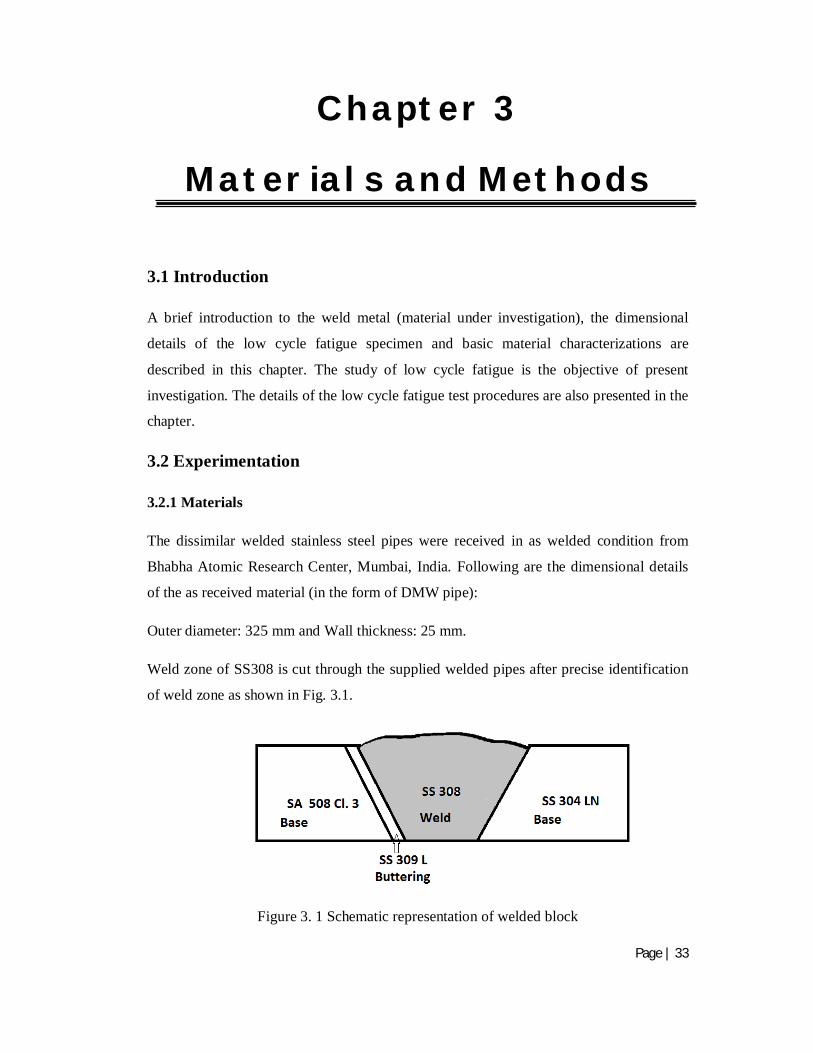
Weld zone of SS308 is cut through the supplied welded pipes after precise identification

of weld zone as shown in Fig. 3.1.

Figure 3. 1 Schematic representation of welded block

Page | 34

3.2.2 Chemical composition

The chemical composition of the weld metal materials was examined using spark optical

emission spectrometer (model: Q6 columbus, Bruker corporation limited, USA).

3.2.3 Microscopic examinations and image analysis

Metallographic specimens of approximately 10 mm 10 mm cross-section or of 10 mm

diameter with 8-10 mm thickness were cut from weld zone of as-received pipes using a

slow speed diamond cutter. The polished specimens were etched with Murakami’s

reagent (10 g KOH, 10 g K3[Fe(CN)6] and 100 ml H2O). Microstructures of the

specimens in all three LR, RC and LC orientations were examined under an optical

microscope (Leica, model: DM 2500 M) and representative photographs were recorded.

The microstructures were also image analysed with the help of Lieca image manager IM

50 software. The ferrite number was measured using Magne Gage as per recomm-

endations of American welding society (AWS) for ferrite number 2-28. The volume

fraction of different phases were measured (repeated over 50 random images) using

Clemex Image Analyzer version PE 3.5.

3.2.4 Hardness measurement

Hardness values of weld SS308 were measured using Vickers hardness testing machine

maintaining indentation load of 30 kgf and dwell time of 5 s (Leco Model, LV 700, MI

USA). Minimum 5 readings were taken for each specimen to obtain the average value.

Tests were performed as per ASTM standard E384[47]. The Vickers hardness was

calculated using the expression:

2

1.854 Pv

avg

HD

Where,

P = indentation load.

1 2

2avgd dD

, in which d1 and d2 are the lengths of two indentation diagonals.

3.2.5 Tensile test

Uniaxial tensile testing of weld zone was performed using flat tensile sub-size specimens

fabricated as per ASTM E8M -2011[1]. Specimens were made from blank using a cut

through pipe as shown in Fig. 3.2 (a) and (b). Specimens are made from pure weld zone,

Page | 35

as mentioned earlier in the thesis study has been carried out for pure weld zone further the

nomenclature LR, LC, and RC represent Longitudinal-Radial (LR), Longitudinal-

Circumferential (LC) and Radial-Circumferential (RC) respectively, and can be

represented during the time of presentation. Furthermore, Fig 3.2 represent plan for

specimen preparation while Fig 4.1 represents microstructure characterisation of different

orientations. Dimensions of sub-size specimen are presented in Fig. 3.3. All tests were

performed at strain rate of 10-3 /sec and data acquisition rate 5 Hz with the help of

universal testing machine (Instron 8862) in ambient environment.

The measurements of strain during the tensile tests were made using an extensometer. At

least three tensile tests were carried out to estimate the average tensile properties. The

load-displacement data were recorded during the tests using the Wave Matrix software

package.

Side view

Top view

Figure 3. 2 Orientation and specimen preparation plan through pipe (a) Side view (b) Top view

Figure 3. 3 Flat tensile subsize weld specimen. All dimensions are in ‘mm’

Page | 36

3.2.6. Low cycle fatigue test

Specimen geometry

Flat tensile sub-size specimen of 8 mm gauge length and 5 mm thickness (as shown in

Fig. 3.4) were fabricated from weld zone maintaining loading axis of the specimen

parallel to the longitudinal dimension of the pipe.

All dimensions are in mm

Test Methodology

All the low cycle fatigue experiments were carried out at room temperature using a 100kN

servo-electric testing system (Instron-8862) supported by Wave Matrix software. The system

was attached to a computer to control the tests as well as for data acquisition. All tests were

conducted in strain control mode till fracture using triangular waveform as per ASTM E 606

[48](as shown in Fig. 3.5) at a constant strain rate of 10-3s-1. The frequency and data

acquisition rate are measured with the help of strain rate and strain amplitude. Resultant set of

hysteresis loops are represented in (Fig. 3.6).

Figure 3. 4 Schematic diagram depicting flat sub size room temperature fatigue specimen

Figure 3. 5 Typical Wave form used for low cycle fatigue test.

Page | 37

-2 -1 0 1 2

-500

0

500

Stre

ss, M

Pa

Strain, %

Hystresis loop

Figure 3. 6 Typical hysteresis loops as generated during experiment

The following parameters were maintained during LCF test:

Frequency = [strain rate / (4 x strain amplitude)] cycles/ s.

Data acquisition rate = Total data points per cycle x frequency

Strain amplitudes = ±0.5%, ±0.7%, ±1.0%, ±1.2% and ±1.5%

Each test was repeated for its conformity. Total 200 data points were collected during each

cycle or stored hysteresis loop. Details of these tests are summarized in Table 3.1.

Table 3. 1 Summary of low cycle fatigue tests

Strain amplitude Nf

Frequency (hertz) (ep) (%)

± 0.5 % 2534 0.0500 0.20631

± 0.7 % 1024 0.0357 0.4392

± 1.0 % 455 0.0250 0.71089

± 1.2 % 402 0.0208 0.89053

± 1.5 % 98 0.0167 1.1501

3.2.7 Fractography

Fracture surfaces of tensile and LCF specimens of various strain amplitudes were

examined using Scanning Electron Microscope (FEG SEM Nova Nano SEM 430).

Page | 38

Chapter 4

4.0 RESULTS AND DISCUSSIONS 4.1 Introduction 4.2 Basic characterization of weld SS 308 4.2.1. Chemical composition 4.2.2. Microstructural evaluation 4.2.3. Hardness 4.3 Tensile test of the metal 4.3.1 Engineering stress strain behaviour 4.3.2 True stress strain behaviour 4.3.3. Fractographic analysis of fracture specimens 4.4 Cyclic deformation behaviour of weld SS 308 4.4.1. Bauschinger effect 4.4.2. Cyclic hardening softening behaviour 4.4.3 Variation of Loop shape parameter 4.4.4. Stability in cyclic stress and strain 4.4.5. Coffin Mansion plot 4.4.6. Variation of total energy with strain amplitude 4.4.7. Cyclic stress strain curve 4.4.8. Comparison of MSSC and CSSC 4.4.9. Masing/ non Masing behaviour 4.4.10. Master curve 4.4.11 Variation of Plastic energy with strain amplitude 4.4.12 Fatigue life estimation 4.4.12.1. Walker model 4.4.12.2. Smith Watson Topper (SWT) model 4.4.13 Fractography of fatigue specimen

Page | 39

Chapter 4

Results and discussions

4.1 Introduction

The chemical composition, microstructural analysis and hardness of weld metal are

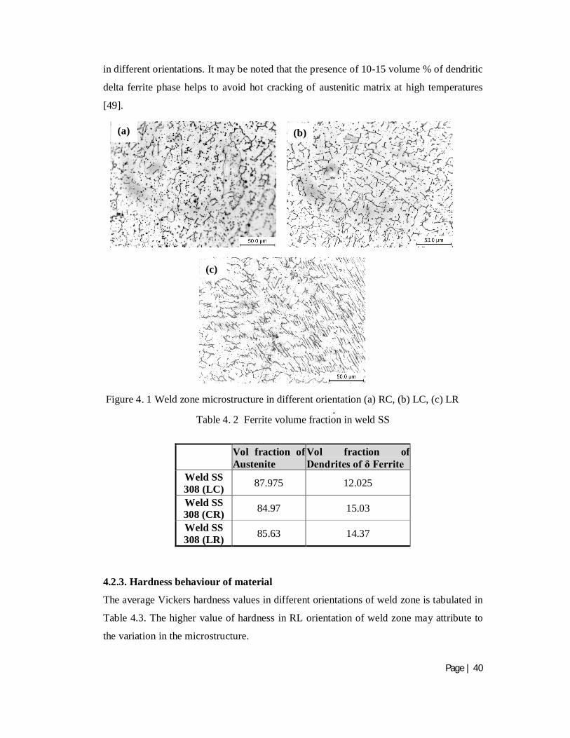
reported in section 4.2. Tensile behaviour of the material are presented and discussed in

section 4.3. The results of the LCF test are presented in section 4.4. The generated data

are analysed and discussed for Bauschinger effect, hardening/ softening behaviour,

Masing / non Masing character, plastic strain energy and fatigue life estimation models.

4.2 Basic characterization of material 4.2.1. Chemical composition

AISI 308 SS is an austenitic grade stainless steel containing 12-27% chromium, 7-25%

nickel and very low amount of carbon. However, weld composition often depends on

process parameters. The chemical composition of weld zone (SS 308) are presented in

Table 4.1 (all in wt. %).

Table 4. 1 Chemical composition of the material

Material Elements (wt. %) C Si Mn P S Cr Mo Ni Co Cu V N Fe Weld SS 308 0.026 0.456 1.045 0.026 0.011 20.797 0.085 9.463 0.046 0.247 0.065 0.073 Rest

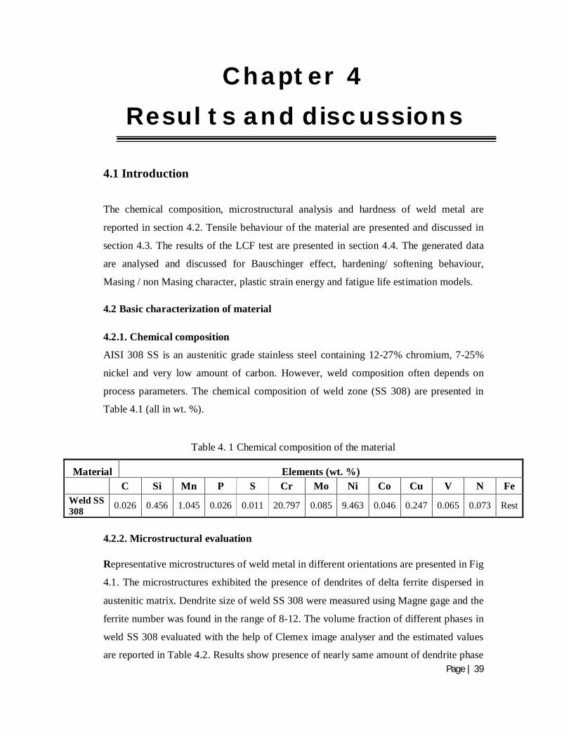
4.2.2. Microstructural evaluation Representative microstructures of weld metal in different orientations are presented in Fig

4.1. The microstructures exhibited the presence of dendrites of delta ferrite dispersed in

austenitic matrix. Dendrite size of weld SS 308 were measured using Magne gage and the

ferrite number was found in the range of 8-12. The volume fraction of different phases in

weld SS 308 evaluated with the help of Clemex image analyser and the estimated values

are reported in Table 4.2. Results show presence of nearly same amount of dendrite phase

Page | 40

in different orientations. It may be noted that the presence of 10-15 volume % of dendritic

delta ferrite phase helps to avoid hot cracking of austenitic matrix at high temperatures

[49].

Table 4.2 Volume fraction of different phases in weld zone Table 4. 2 Ferrite volume fraction in weld SS

4.2.3. Hardness behaviour of material

The average Vickers hardness values in different orientations of weld zone is tabulated in

Table 4.3. The higher value of hardness in RL orientation of weld zone may attribute to

the variation in the microstructure.

Vol fraction of Austenite

Vol fraction of Dendrites of δ Ferrite

Weld SS 308 (LC) 87.975 12.025

Weld SS 308 (CR) 84.97 15.03

Weld SS 308 (LR) 85.63 14.37

Figure 4. 1 Weld zone microstructure in different orientation (a) RC, (b) LC, (c) LR

(a) (b)

(c)

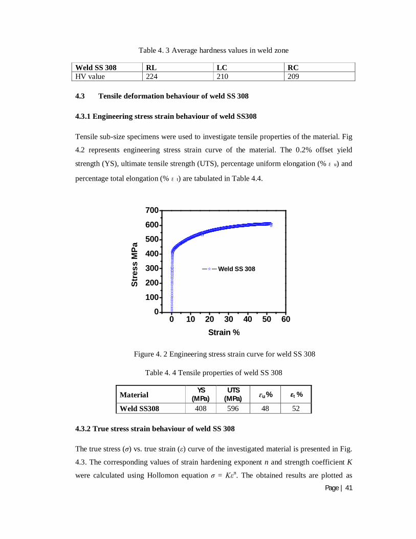
Page | 41

Table 4. 3 Average hardness values in weld zone

Weld SS 308 RL LC RC HV value 224 210 209 4.3 Tensile deformation behaviour of weld SS 308 4.3.1 Engineering stress strain behaviour of weld SS308 Tensile sub-size specimens were used to investigate tensile properties of the material. Fig

4.2 represents engineering stress strain curve of the material. The 0.2% offset yield

strength (YS), ultimate tensile strength (UTS), percentage uniform elongation (%εu) and

percentage total elongation (%εt) are tabulated in Table 4.4.

Table 4. 4 Tensile properties of weld SS 308

Material YS (MPa)

UTS (MPa) ɛu % ɛt %

Weld SS308 408 596 48 52 4.3.2 True stress strain behaviour of weld SS 308 The true stress (σ) vs. true strain (ε) curve of the investigated material is presented in Fig.

4.3. The corresponding values of strain hardening exponent n and strength coefficient K

were calculated using Hollomon equation σ = Kεn. The obtained results are plotted as

0 10 20 30 40 50 600

100

200

300

400

500

600

700

Stre

ss M

Pa

Strain %

Weld SS 308

Figure 4. 2 Engineering stress strain curve for weld SS 308

Page | 42

ln (true stress) vs. ln (true strain) in the pcslastic domain which results into straight lines

as shown in Fig. 4.3. The values of n was estimated from the slope of the plot and the

strength coefficient, K values was obtained from the intercept of this plot to the stress axis

at ε = 1.

-3 -2 -1

6.3

6.6

ln(T

rue

stre

ss) M

Pa

ln (True strain)

R2=0.9959n= 0.327K= 1170 MPa

Figure 4. 3 True stress strain curve for weld SS 308

4.3.3. Fractographic analysis of tensile specimens

The fractographs of tensile specimens of weld metal are presented in Fig 4.4. The figure

shows presence of dimples and micro voids which indicates the ductile mode of fracture.

Figure 4. 4 Fractograph of post tensile weld SS 308 specimen

Page | 43

-2 -1 0 1 2 3

-500

0

500

Strain Amplitude 1.2% Sample 10Bauschinger effect parameter p= p= 0.8476

r= 168.934

r= 0.232136

Bauschinger Stress l= p-r/p= 0.663

Bauschinger Stress r/ p = 0.8947

Stre

ss M

Pa

Strain %

The micromechanism of ductile fracture consists of initiation of voids, their growth and

coalescence.These voids initiate from inclusions, precipitates, second phase particles, etc.,

in the metallic matrix and grow further under the influence of hydrostatic stress and

plastic strain [50].

4.4 Cyclic deformation behaviour of weld SS 308

This section provides us insight of materials inelastic behaviour by studying certain

aspects of cyclic deformation behaviour such as Bauschinger effect, cyclic

hardening/softening, cyclic stress strain curve and Masing-nonMasing behaviour etc..

4.4.1 Bauschinger effect

A material under uniaxial loading unloading regime in plastic region shows substantial

decrement in reversed yield stress [51]. Therefore, the material may yield at lower stress

levels during reloading in reverse direction (compression) [39]. Fig 4.5 shows typical

diagram depicting Bauschinger effect. In the present investigation two established

parameters i.e., Bauschinger strain and Bauschinger stress are evaluated to quantify this

effect. The stress parameter (βσ1) to represent Bauschinger effect can be expressed as

lpyrp

Where, p is the maximum stress and yr is the yield stress in reverse direction.

Bauschinger strain can be defined as the plastic strain on stress reversal at 75% of the

maximum tensile stress in the forward direction.

Figure 4. 5 Schematic diagram depicting Bauschinger effect

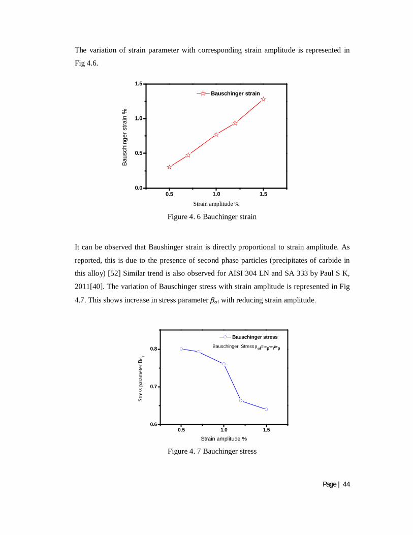
Page | 44

0.5 1.0 1.50.0

0.5

1.0

1.5

Bau

schi

nger

stra

in %

Strain amplitude %

Bauschinger strain

0.5 1.0 1.50.6

0.7

0.8 Bauschinger Stress l= p-r/p

Stre

ss p

aram

eter

B l

Strain amplitude %

Bauschinger stress

The variation of strain parameter with corresponding strain amplitude is represented in

Fig 4.6.

It can be observed that Baushinger strain is directly proportional to strain amplitude. As

reported, this is due to the presence of second phase particles (precipitates of carbide in

this alloy) [52] Similar trend is also observed for AISI 304 LN and SA 333 by Paul S K,

2011[40]. The variation of Bauschinger stress with strain amplitude is represented in Fig

4.7. This shows increase in stress parameter l with reducing strain amplitude.

Figure 4. 7 Bauchinger stress

Figure 4. 6 Bauchinger strain

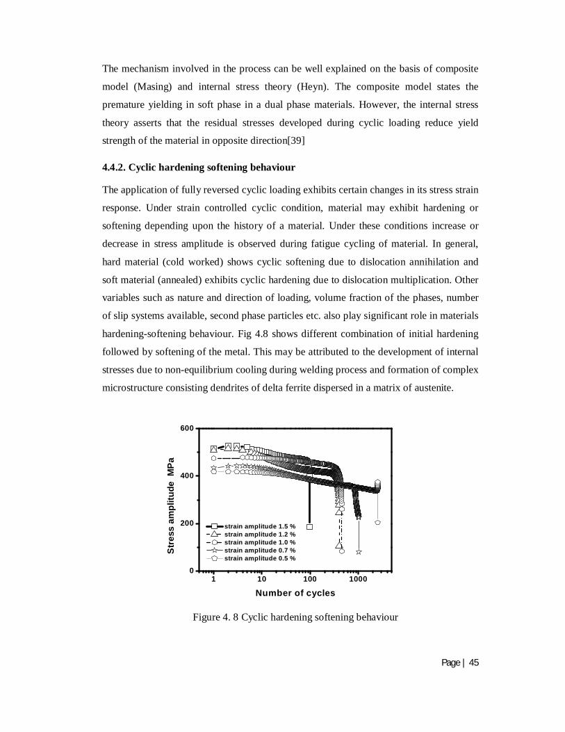
Page | 45

The mechanism involved in the process can be well explained on the basis of composite

model (Masing) and internal stress theory (Heyn). The composite model states the

premature yielding in soft phase in a dual phase materials. However, the internal stress

theory asserts that the residual stresses developed during cyclic loading reduce yield

strength of the material in opposite direction[39]

4.4.2. Cyclic hardening softening behaviour

The application of fully reversed cyclic loading exhibits certain changes in its stress strain

response. Under strain controlled cyclic condition, material may exhibit hardening or

softening depending upon the history of a material. Under these conditions increase or

decrease in stress amplitude is observed during fatigue cycling of material. In general,

hard material (cold worked) shows cyclic softening due to dislocation annihilation and

soft material (annealed) exhibits cyclic hardening due to dislocation multiplication. Other

variables such as nature and direction of loading, volume fraction of the phases, number

of slip systems available, second phase particles etc. also play significant role in materials

hardening-softening behaviour. Fig 4.8 shows different combination of initial hardening

followed by softening of the metal. This may be attributed to the development of internal

stresses due to non-equilibrium cooling during welding process and formation of complex

microstructure consisting dendrites of delta ferrite dispersed in a matrix of austenite.

1 10 100 10000

200

400

600

Stre

ss a

mpl

itude

MPa

Number of cycles

strain amplitude 1.5 % strain amplitude 1.2 % strain amplitude 1.0 % strain amplitude 0.7 % strain amplitude 0.5 %

Figure 4. 8 Cyclic hardening softening behaviour

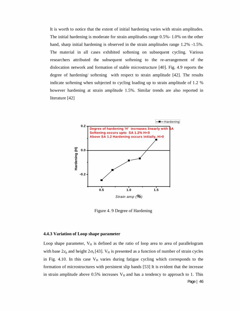
Page | 46

0.5 1.0 1.5

-0.2

0.0

0.2

Har

deni

ng (H

)

Strain amp (%)

Hardening

Degree of hardening 'H' increases linearly with SASoftening occurs upto SA 1.2% H<0Above SA 1.2 Hardening occurs initially, H>0

It is worth to notice that the extent of initial hardening varies with strain amplitudes.

The initial hardening is moderate for strain amplitudes range 0.5%- 1.0% on the other

hand, sharp initial hardening is observed in the strain amplitudes range 1.2% -1.5%.

The material in all cases exhibited softening on subsequent cycling. Various

researchers attributed the subsequent softening to the re-arrangement of the

dislocation network and formation of stable microstructure [40]. Fig. 4.9 reports the

degree of hardening/ softening with respect to strain amplitude [42]. The results

indicate softening when subjected to cycling loading up to strain amplitude of 1.2 %

however hardening at strain amplitude 1.5%. Similar trends are also reported in

literature [42]

4.4.3 Variation of Loop shape parameter

Loop shape parameter, VH is defined as the ratio of loop area to area of parallelogram

with base 2p and height 2a [43]. VH is presented as a function of number of strain cycles

in Fig. 4.10. In this case VH varies during fatigue cycling which corresponds to the

formation of microstructures with persistent slip bands [53] It is evident that the increase

in strain amplitude above 0.5% increases VH and has a tendency to approach to 1. This

Figure 4. 9 Degree of Hardening

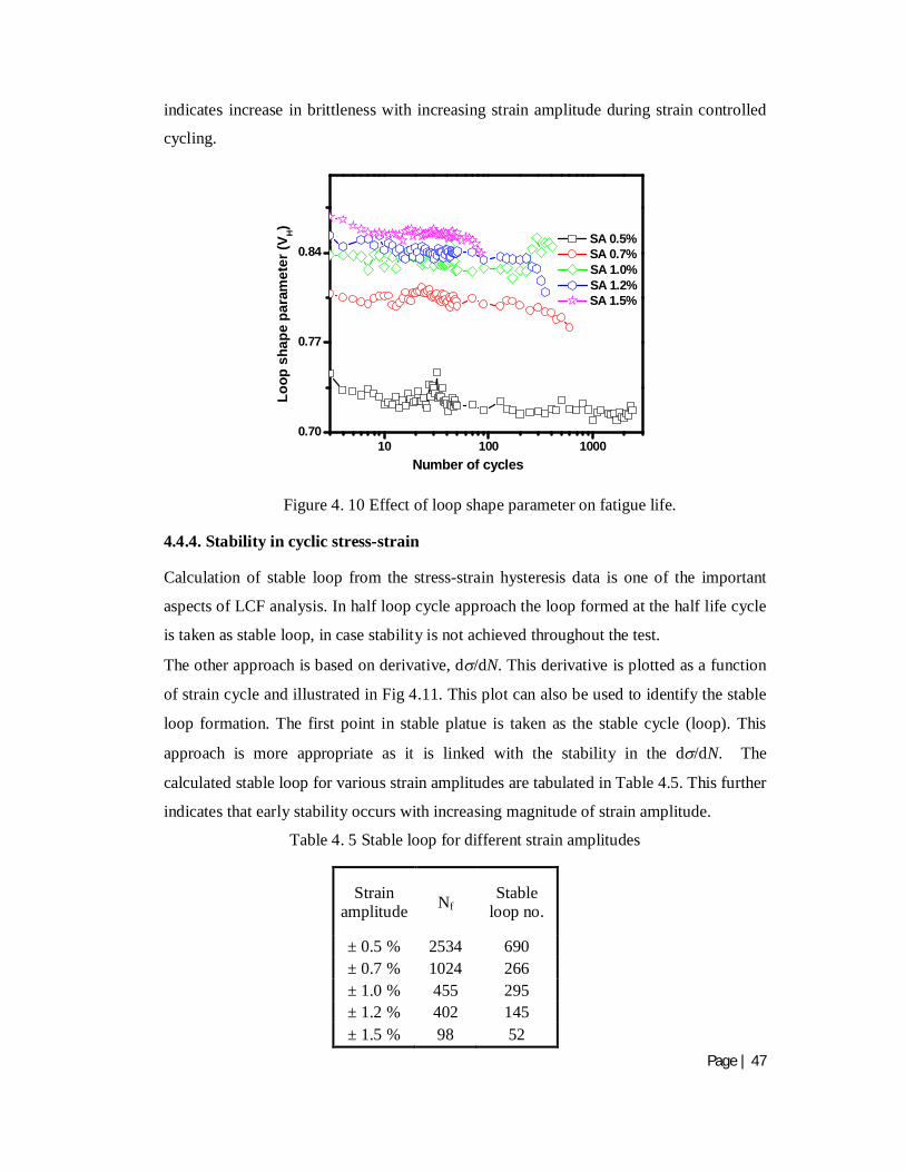
Page | 47

indicates increase in brittleness with increasing strain amplitude during strain controlled

cycling.

4.4.4. Stability in cyclic stress-strain

Calculation of stable loop from the stress-strain hysteresis data is one of the important

aspects of LCF analysis. In half loop cycle approach the loop formed at the half life cycle

is taken as stable loop, in case stability is not achieved throughout the test.

The other approach is based on derivative, d/dN. This derivative is plotted as a function

of strain cycle and illustrated in Fig 4.11. This plot can also be used to identify the stable

loop formation. The first point in stable platue is taken as the stable cycle (loop). This

approach is more appropriate as it is linked with the stability in the d/dN. The

calculated stable loop for various strain amplitudes are tabulated in Table 4.5. This further

indicates that early stability occurs with increasing magnitude of strain amplitude.

Table 4. 5 Stable loop for different strain amplitudes

Strain amplitude Nf

Stable loop no.

± 0.5 % 2534 690 ± 0.7 % 1024 266 ± 1.0 % 455 295 ± 1.2 % 402 145 ± 1.5 % 98 52

Figure 4. 10 Effect of loop shape parameter on fatigue life.

10 100 10000.70

0.77

0.84

Loop

sha

pe p

aram

eter

(VH)

Number of cycles

SA 0.5% SA 0.7% SA 1.0% SA 1.2% SA 1.5%

Page | 48

1 10 100 1000 10000-200-150-100-50

050

-150

-100

-50

0-200-150-100-50

050

-140

-70

0

-200

-100

0

1 10 100 1000 10000

d(

) / d

(N)

Number of cycles

(SA 0.5%)

(SA 0.7%)

(SA 1.0%)

(SA 1.2%)

(SA 1.5%)

Figure 4. 11 Cyclic stability curve 4.4.5. Coffin Mansion plot

The Coffin Mansion plot i.e., plastic strain amplitude vs. number of cycles to failure plot

is presented in Fig. 4.12 [37]. The estimated value of fatigue ductility coefficient (f′) and

fatigue ductility exponent (c) from the figure are 1.29786 and -0.51532 respectively.

These results are in line with the reported work [37].

Figure 4. 12 Coffin Mansion plot

100 1000 100000.0

0.4

0.8

1.2

plas

tic s

trai

n am

plitu

de (

p %)

Cycles to failure

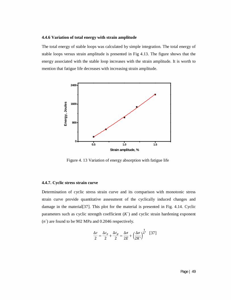
Page | 49

4.4.6 Variation of total energy with strain amplitude

The total energy of stable loops was calculated by simple integration. The total energy of

stable loops versus strain amplitude is presented in Fig 4.13. The figure shows that the

energy associated with the stable loop increases with the strain amplitude. It is worth to

mention that fatigue life decreases with increasing strain amplitude.

4.4.7. Cyclic stress strain curve

Determination of cyclic stress strain curve and its comparison with monotonic stress

strain curve provide quantitative assessment of the cyclically induced changes and

damage in the material[37]. This plot for the material is presented in Fig. 4.14. Cyclic

parameters such as cyclic strength coefficient (K´) and cyclic strain hardening exponent

(n´) are found to be 902 MPa and 0.2046 respectively.

[37]

0.5 1.0 1.50

800

1600

2400

Ener

gy, J

oule

s

Strain amplitude, %

Figure 4. 13 Variation of energy absorption with fatigue life

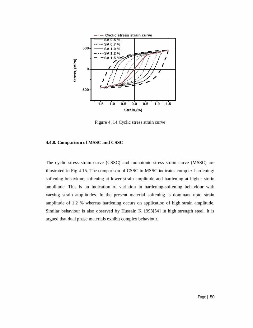
Page | 50

-1.5 -1.0 -0.5 0.0 0.5 1.0 1.5

-500

0

500

Stre

ss, (

MPa

)

Strain,(%)

Cyclic stress strain curve SA 0.5 % SA 0.7 % SA 1.0 % SA 1.2 % SA 1.5 %

Figure 4. 14 Cyclic stress strain curve

4.4.8. Comparison of MSSC and CSSC

The cyclic stress strain curve (CSSC) and monotonic stress strain curve (MSSC) are

illustrated in Fig 4.15. The comparison of CSSC to MSSC indicates complex hardening/

softening behaviour, softening at lower strain amplitude and hardening at higher strain

amplitude. This is an indication of variation in hardening-softening behaviour with

varying strain amplitudes. In the present material softening is dominant upto strain

amplitude of 1.2 % whereas hardening occurs on application of high strain amplitude.

Similar behaviour is also observed by Hussain K 1993[54] in high strength steel. It is

argued that dual phase materials exhibit complex behaviour.

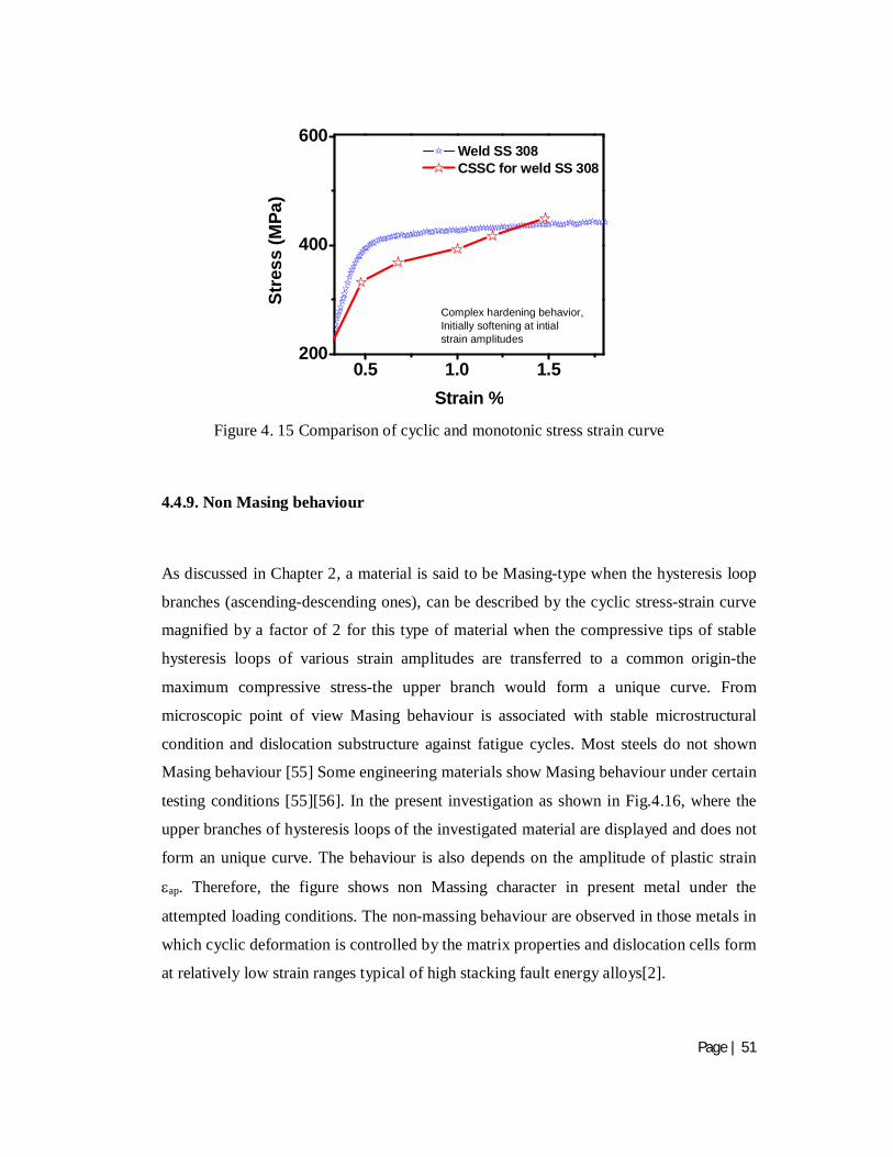
Page | 51

4.4.9. Non Masing behaviour

As discussed in Chapter 2, a material is said to be Masing-type when the hysteresis loop

branches (ascending-descending ones), can be described by the cyclic stress-strain curve

magnified by a factor of 2 for this type of material when the compressive tips of stable

hysteresis loops of various strain amplitudes are transferred to a common origin-the

maximum compressive stress-the upper branch would form a unique curve. From

microscopic point of view Masing behaviour is associated with stable microstructural

condition and dislocation substructure against fatigue cycles. Most steels do not shown

Masing behaviour [55] Some engineering materials show Masing behaviour under certain

testing conditions [55][56]. In the present investigation as shown in Fig.4.16, where the

upper branches of hysteresis loops of the investigated material are displayed and does not

form an unique curve. The behaviour is also depends on the amplitude of plastic strain

ap. Therefore, the figure shows non Massing character in present metal under the

attempted loading conditions. The non-massing behaviour are observed in those metals in

which cyclic deformation is controlled by the matrix properties and dislocation cells form

at relatively low strain ranges typical of high stacking fault energy alloys[2].

0.5 1.0 1.5200

400

600

Stre

ss (M

Pa)

Strain %

Weld SS 308 CSSC for weld SS 308

Complex hardening behavior, Initially softening at intial strain amplitudes

Figure 4. 15 Comparison of cyclic and monotonic stress strain curve

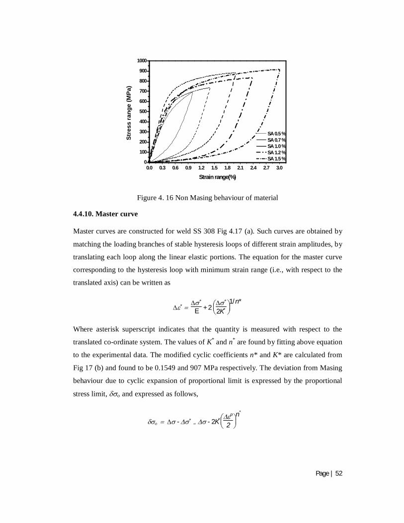
Page | 52

0.0 0.3 0.6 0.9 1.2 1.5 1.8 2.1 2.4 2.7 3.00

100

200

300

400

500

600

700

800

900

1000

SA 0.5 % SA 0.7 % SA 1.0 % SA 1.2 % SA 1.5 %

Stre

ss ra

nge

(MPa

)

Strain range(%)

Figure 4. 16 Non Masing behaviour of material

4.4.10. Master curve

Master curves are constructed for weld SS 308 Fig 4.17 (a). Such curves are obtained by

matching the loading branches of stable hysteresis loops of different strain amplitudes, by

translating each loop along the linear elastic portions. The equation for the master curve

corresponding to the hysteresis loop with minimum strain range (i.e., with respect to the

translated axis) can be written as

E + 2

2K1/n*

Where asterisk superscript indicates that the quantity is measured with respect to the

translated co-ordinate system. The values of K* and n* are found by fitting above equation

to the experimental data. The modified cyclic coefficients n* and K* are calculated from

Fig 17 (b) and found to be 0.1549 and 907 MPa respectively. The deviation from Masing

behaviour due to cyclic expansion of proportional limit is expressed by the proportional

stress limit,and expressed as follows,

- - 2K*

p

2

n*

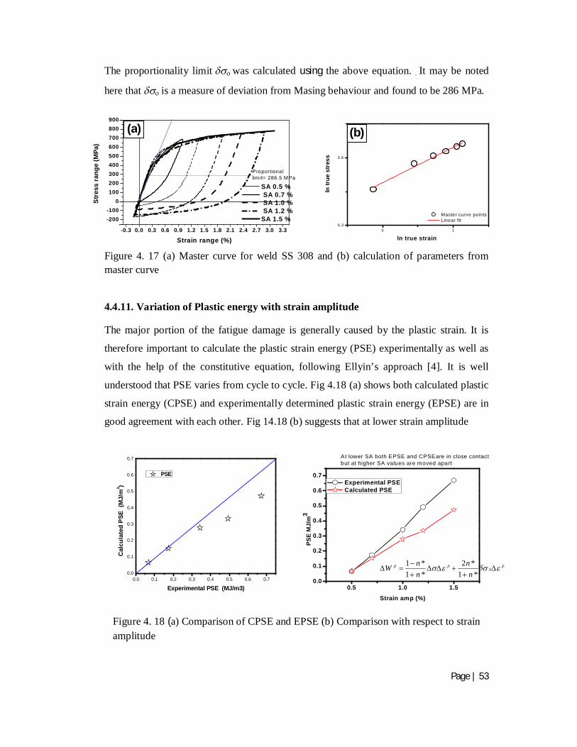
Page | 53

The proportionality limitwas calculated using the above equation. It may be noted

here that is a measure of deviation from Masing behaviour and found to be 286 MPa.

Figure 4. 17 (a) Master curve for weld SS 308 and (b) calculation of parameters from master curve

4.4.11. Variation of Plastic energy with strain amplitude

The major portion of the fatigue damage is generally caused by the plastic strain. It is

therefore important to calculate the plastic strain energy (PSE) experimentally as well as

with the help of the constitutive equation, following Ellyin’s approach [4]. It is well

understood that PSE varies from cycle to cycle. Fig 4.18 (a) shows both calculated plastic

strain energy (CPSE) and experimentally determined plastic strain energy (EPSE) are in

good agreement with each other. Fig 14.18 (b) suggests that at lower strain amplitude

0.5 1.0 1.50.0

0.1

0.2

0.3

0.4

0.5

0.6

0.7

1 * 2 *1 * 1 *

p p po

n nWn n

PSE

MJ/

m3

Strain amp (%)

Experimental PSE Calculated PSE

At lower SA both EPSE and CPSEare in close contact but at higher SA values are moved apart

Figure 4. 18 (a) Comparison of CPSE and EPSE (b) Comparison with respect to strain amplitude

-0.3 0.0 0.3 0.6 0.9 1.2 1.5 1.8 2.1 2.4 2.7 3.0 3.3

-200-100

0100200300400500600700800900

Stre

ss ra

nge

(MPa

)

Strain range (%)

SA 0.5 % SA 0.7 % SA 1.0 % SA 1.2 % SA 1.5 %

Proportional lim it= 286.5 MPa

0 16.3

6.6

ln tr

ue s

tres

s

ln true strain

Master curve points Linear fit

(b) (a)

0.0 0.1 0.2 0.3 0.4 0.5 0.6 0.70.0

0.1

0.2

0.3

0.4

0.5

0.6

0.7

Cal

cula

ted

PSE

(MJ/

m3 )

Experimental PSE (MJ/m3)

PSE

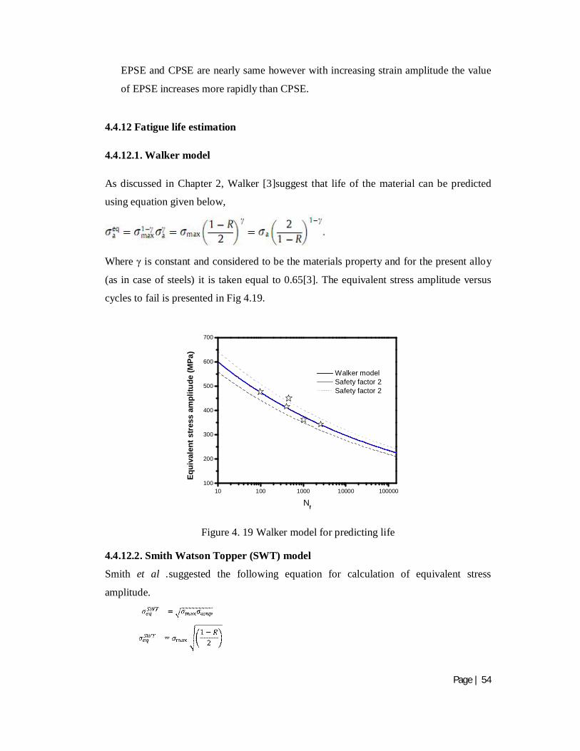
Page | 54

EPSE and CPSE are nearly same however with increasing strain amplitude the value

of EPSE increases more rapidly than CPSE.

4.4.12 Fatigue life estimation 4.4.12.1. Walker model As discussed in Chapter 2, Walker [3]suggest that life of the material can be predicted

using equation given below,

Where γ is constant and considered to be the materials property and for the present alloy

(as in case of steels) it is taken equal to 0.65[3]. The equivalent stress amplitude versus

cycles to fail is presented in Fig 4.19.

Figure 4. 19 Walker model for predicting life

4.4.12.2. Smith Watson Topper (SWT) model

Smith et al .suggested the following equation for calculation of equivalent stress

amplitude.

10 100 1000 10000 100000100

200

300

400

500

600

700

Equi

vale

nt s

tres

s am

plitu

de (M

Pa)

Nf

Walker model Safety factor 2 Safety factor 2

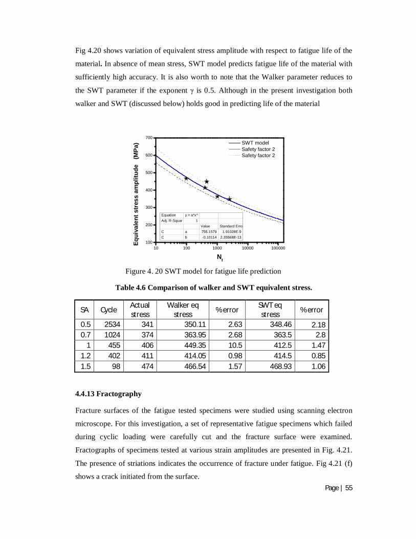
Page | 55

Fig 4.20 shows variation of equivalent stress amplitude with respect to fatigue life of the

material. In absence of mean stress, SWT model predicts fatigue life of the material with

sufficiently high accuracy. It is also worth to note that the Walker parameter reduces to

the SWT parameter if the exponent γ is 0.5. Although in the present investigation both

walker and SWT (discussed below) holds good in predicting life of the material

Table 4.6 Comparison of walker and SWT equivalent stress.

SA Cycle Actual stress

Walker eq stress % error SWT eq

stress % error

0.5 2534 341 350.11 2.63 348.46 2.18 0.7 1024 374 363.95 2.68 363.5 2.8

1 455 406 449.35 10.5 412.5 1.47 1.2 402 411 414.05 0.98 414.5 0.85 1.5 98 474 466.54 1.57 468.93 1.06

4.4.13 Fractography

Fracture surfaces of the fatigue tested specimens were studied using scanning electron

microscope. For this investigation, a set of representative fatigue specimens which failed

during cyclic loading were carefully cut and the fracture surface were examined.

Fractographs of specimens tested at various strain amplitudes are presented in Fig. 4.21.

The presence of striations indicates the occurrence of fracture under fatigue. Fig 4.21 (f)

shows a crack initiated from the surface.

10 100 1000 10000 100000100

200

300

400

500

600

700

Eq

uiva

lent

str

ess

ampl

itude

(M

Pa)

Nf

SWT model Safety factor 2 Safety factor 2

Equation y = a*x^Adj. R-Squar 1

Value Standard ErroC a 755.1579 1.91028E-9C b -0.10114 2.35568E-13

Figure 4. 20 SWT model for fatigue life prediction

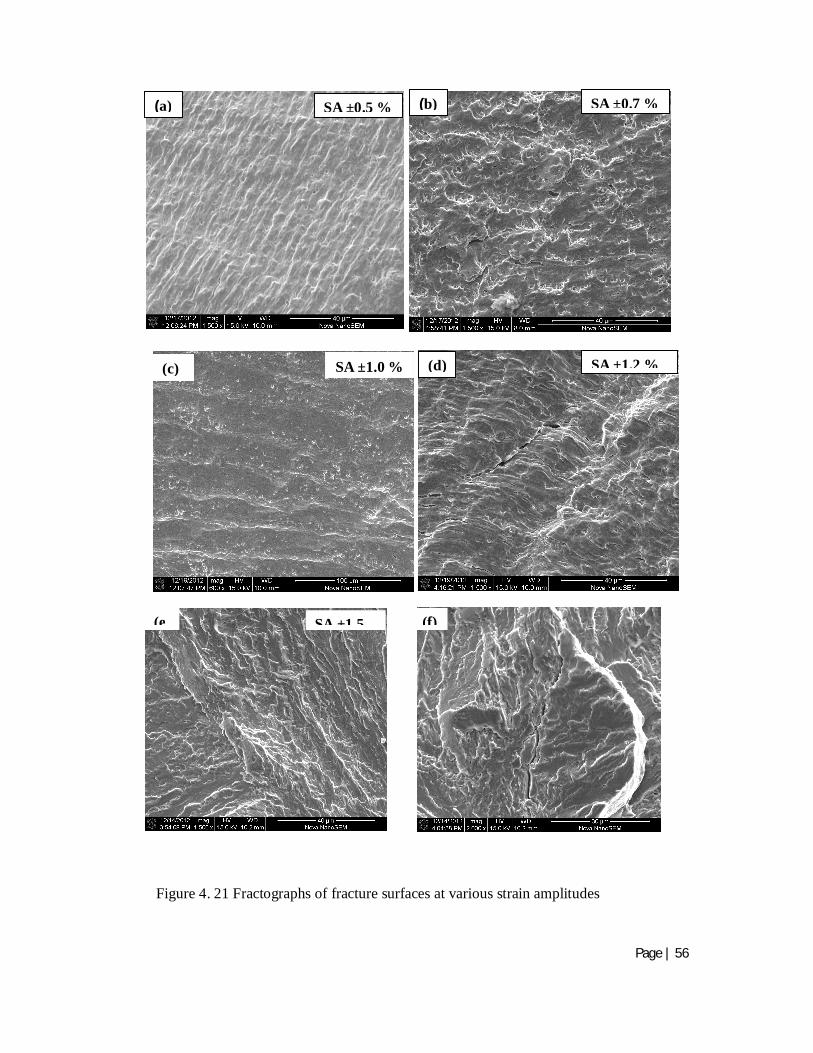
Page | 56

(d) SA ±1.2 % (c) SA ±1.0 %

(b) SA ±0.7 % (a) SA ±0.5 %

Figure 4. 21 Fractographs of fracture surfaces at various strain amplitudes

(e SA ±1.5 (f)

Page | 57

Chapter 5

5.0 Conclusions and Suggestions for future work

5.1 Conclusions 5.2 Suggestion for future work

Page | 58

Chapter 5

Conclusions and Suggestions for future

work

5.1 Conclusions

Present investigation leads to following conclusions:

Significant directionality of strain hardening is observed in the present metal under

applied strain controlled cycling indicating pronounced Bauschinger effect.

The initial hardening and subsequent softening during strain cycling is observed in

the metal.

Hardening factor and Loop shape parameter indicate that material exhibits softening

up to strain amplitude of 1.2 % and followed by hardening at higher strain

amplitudes.

Comparison of cyclic and monotonic stress strain curve conforms initial softening

and subsequent hardening in the material.

Material exhibits non Masing behaviour under present conditions.

Calculated and experimentally determined plastic stain energy are in good agreement

with each other.

Both SWT and Walker models holds good for predicting fatigue life of the material

5.2 Scope for future work Low cycle fatigue behaviour of weld zone at elevated temperature of 285◦C

Optical and transmission electron microscopic studies may be useful to enhance the

understanding of involved micro mechanisms.

Page | 59

References [1] ASTM E 8M, 2011, Standard test methods for tension testing of metallic

materials, Annual book of ASTM standards,ASTM International.

[2] Ellyin F. Fatigue damage crack growth and life prediction, Springer, 1996.

[3] Dowling N E. Mean stress effects in stress-life and strain-life fatigue, ASM Internatioal, 56 (2004).

[4] Ellyin F, Kujawski D. Plastic strain energy in fatigue, Journal of Pressure Vessel Technology, 106 (1984).

[5] International Energy Agency, 2011, Report on Indian energy requirements, Energy Information Administration.

[6] Miteva R, Taylor N G. General review of dissimilar metal welds in piping systems of pressurised water reactors Including WWER designs, European energy commision, 22470EN (2006).

[7] Rie K, Portella P D. Low cycle fatigue and elasto- plastic behaviour of materials, Elsevier, 1998.

[8] Paventhan R, Lakshminarayanan P R, Balasubramanian V. Fatigue behaviour of friction welded medium carbon steel and austenitic stainless steel dissimilar joints, Materials & Design, 32 ( 2011).

[9] Cao J, Gong Y, Zhu K, Yang Z G, Luo X M, Gu F M. Microstructure and mechanical properties of dissimilar materials joints between T92 martensitic and S304h austenitic steels, Materials & Design, 32 (2011).

[10] Arora P, Sivaprasad S. Fatigue studies on stainless steel piping materials and components : Indian AHWR, Transactions. SMIRT, BARC, Mumbai, (2011).

11] ANSI/ASME B36 19M, Stainless steel pipe, ASME International, 1994.

[12] Lippold J C, Kotecki D J. Welding metallurgy and weldability of stainless steels, Canada Wiley A John, 2005.

[13] Race J M. Carbon diffusion across dissimilar steel welds. Cambridge. 1992.

[14] Bhattacharya D K. Failures of welded joints, Proceedings  COFA-1997 NML Jamshedpur, 1 (1997).

Page | 60

[15] Kuwabara K, Takahashi Y, Kawaguchi S, Fukuda Y, Fukakura J. Fatigue strength of dissimilar welded joints for the main vessel of an LMFBR, Nuclear Engineering and Design, 133 (1992).

[16] Nelson T W, Lippold J C, Miller M J. Nature and evolution of the fusion boundary in ferritic-austenitic dissimilar weld metals Part 1-Nucleation and growth, AWS Welding Research, Oct (1999).

[17] Celik A, Alsaran A. Mechanical and structural properties of similar and dissimilar steel joints, Material Charecterisation, 5803 (1999).

[18] Laha K, Chandravathi K S, Rao K B S, Mannan S L. An assessment of creep deformation and fracture behavior of 2.25Cr-1Mo similar and dissimilar weld joints, Metallurgical And Materials Transactions A, 32 A (2001).

[19] Bhandari S, Dubois D, Guichard D. Behaviour of a PWR vessel dissimilar metal weld during a steam line break transient, Nuclear Engineering and Design, 207 (2001).

[20] Faidy C, Martin G, Chapuliot S, Kayser Y, Safa N, Cipierre M F, Gilles P. Assessment of aged piping dissimilar metal weld integrity ( ADIMEW ), Proceedings of FISA conference, Luxembourg, (2003).

[21] Kusko C S, Dupont J N, Marder A R. The influence of microstructure on fatigue crack propagation behavior of stainless steel welds, AWS Welding Journal, 5 (2004).

[22] Keehan E, Effect of microstructure on mechanical properties of high strength steel weld metals, Chalmers University of Technology, 2004.

[23] Kaçar R, Baylan O. An investigation of microstructure/property relationships in dissimilar welds between martensitic and austenitic stainless steels, Materials & Design, 35 (2004).

[24] Ravi S, Balasubramanian V, Nemat Nasser S. Effect of mis-match ratio (MMR) on fatigue crack growth behaviour of HSLA steel welds, Engineering Failure Analysis, 11 (2004).

[25] Lee D G, Jang K C, Kuk J M, Kim I S. Fatigue properties of inertia dissimilar friction-welded stainless steels, Journal of Materials Processing Technology, 11 (2004).

[26] Sireesha M, Albert S K, Sundaresan S, Influence of high-temperature exposure on the microstructure and mechanical properties of dissimilar metal welds between modified 9Cr-1Mo steel and alloy 800, Metallurgical And Materials Transactions A, 36 (2005).

[27] Cui Y, Lundin C D. Effect of microfissures on fatigue properties of austenitic stainless steel weld metals, Materials Letters, 59 (2005).

Page | 61

[28] Satyanarayana V V, Madhusudhan Reddy G, Mohandas T. Dissimilar metal friction welding of austenitic–ferritic stainless steels, Journal of Materials Processing Technology 160 (2005).

[29] Madhusudhan Reddy G, Mohandas T, Sambasiva Rao A, Satyanarayana V V. Influence of welding processes on microstructure and mechanical properties of dissimilar austenitic-ferritic stainless steel welds, Materials and Manufacturing Processes, 20 (2005).

[30] Dupont Y J N, Kusko C S. Technical note on Martensite formation in austenitic/ ferritic dissimilar alloy welds, AWS Welding Journal, 52 (2007).

[31] Kim J, Lee S. A study on structural integrity of dissimilar welds in nuclear piping, Transactions SMIRT Torrento, 19 (2007).

[32] Jang C, Lee J, Sung K J, Eun Jin T. Mechanical property variation within inconel 82/182 dissimilar metal weld between low alloy steel and 316 stainless steel, International Journal of Pressure Vessels and Piping, 85 (2008).

[33] Kim J W, Lee K, Kim J S, Byun T S. Local mechanical properties of alloy 82/182 dissimilar weld joint between SA508 Gr.1A and F316 SS at RT and 320°C, Journal of Nuclear Materials, 384 (2009).

[34] Krishnaprasad K, Prakash R V. Fatigue crack growth behavior in dissimilar metal weldment of stainless steel and carbon steel. World Academy of Science. Engineering and Technology, 56 (2009).

[35] Hasan M M, Abadi M P. Correlation between macro/micro structure and mechanical properties of dissimilar resistance spot welds of AISI 304 austenitic stainless steel and AISI 1008 low carbon steel, Association of Metallurgical Engineers of Serbia AMES, 16 (2010).

[36] Samal M K, Dutta B K, Kushwaha H S. A study on ductile fracture initiation in the pht piping material of an indian PHWR using local approach, International Journal of Pressure Vessels and Piping, 76 (1999).

[37] Dieter G E. Mechanical metallurgy, MacGraw- Hill Book Company, 1996.

[38] Suresh S. Fatigue in materials, Cambridge University Press, 1998.

[39] Yan J. Study of Bauschinger effect in various spring steels, University of Toronto. 1998.

[40] Paul S K. Experimentation and material modelling for cyclic plastic deformation behavior in primary heat transport piping (PHT) materials. Jadavpur University. Kolkata, 2011.

[41] Shang H, Ding H J. Low cycle fatigue stress-strain relation model of cyclic hardening or cyclic softening factor, Engineering Fracture Mechanics, 54 (1996).

Page | 62

[42] Ye D, Matsuoka S, Nagashima N, Suzuki N. The low-cycle fatigue, deformation and final fracture behaviour of an austenitic stainless steel, Materials Science and Engineering A, 415 (2006).

[43] Polák J, Obrtlik K, Hajek M. Cyclic plasticity in type 316l austenitic stainless steel, Fatigue Fracture Engineering Material Structures, 17 (1994).

[44] Morrison D J, Jia Y, Moosbrugger J C. Cyclic plasticity of nickel at low plastic strain amplitude . hysteresis loop shape analysis, Materials Science and Engineering A, 314 (2001).

[45] Dutta K. Accumulation of ratcheting strain in polycrystalline metallic materials, IIT Kharagpur, 2012.

[46] Branco R, Costa J D, Antunes F V. Low-cycle fatigue behaviour of 34CrNiMo6 high strength steel, Theoretical and Applied Fracture Mechanics, 58 (2012).

[47] ASTM E 384, 2011, Standard test method for knoop and vickers hardness of materials, Annual book of ASTM standards,ASTM International.

[48] ASTM E 606, 2011, Standard practice for strain-controlled fatigue testing. Annual book of ASTM standards,ASTM International.

[49] David S A, Vitek J M, Alexander D J. Embrittlement of austenitic stainless steel welds, 1995.

[50] Das A, Tarafder S. Geometry of dimples and its correlation with mechanical properties in austenitic stainless steel, Scripta Materialia, 59 (2008).

[51] Neel C G, Bobet V, Clavel M. Cyclic deformation behaviour and Bauschinger effect in ductile cast iron, Materials Science and Engineering A, 272 (2008).

[52] Plumtree A, Raouf H A. Cyclic stress strain response and substructure, International Journal of Fatigue, 23 (1998).

[53] Saad A A. Cyclic plasticity and creep of power plant materials, University of Nottingham, 2012.

[54] Hussain K. Monotonic and cyclic stress strain behavior of a high strength steel, Metallurgical Science and Technology, 11 (1993).

[55] Jiang Y, Zhang J. Benchmark experiments and characteristic cyclic plasticity deformation. International Journal of Plasticity, 24 (2008).

[56] Halama R, Sedlak J, Sofer M. Phenomenological modelling of cyclic plasticity. Intech International, 1 (2012).

[57] Dutta A, Material charecterisation of SS316 for low cycle fatigue damage, Jadavpur University, (2009)

Page | 63

BIO-DATA Name Abhishek Chaturvedi Date of birth 04.05.1988

Permanent Address Bewar road, Bholepur, Fatehgarh Disst- Farrukhabad Uttar Pradesh, 209625

E-mail ID [email protected] Languages Known Hindi, English

EDUCATIONAL QUALIFICATION Examination Discipline/

Specialization

School/college Board/

University

Year of Passing

Percentile

M. Tech (Research)


NIT Rourkela National Institute of Technology Rourkela

2013 9.12* (CGPA)

B. Tech. Metallurgical and Materials Engineering

UIET, CSJM University kanpur.

CSJM University

2010 8.45 (CGPA)

HSSC Maths, Physics, Chemistry

Central School Fatehgarh

CBSE 2005 62 %

HighSchool Central School Fatehgarh.

CBSE 2003 78 %

PROJECT DETAILS M. Tech (Research)

Low Cycle Fatigue Behaviour of AISI 308 Stainless Steel Weld Metal .

Conference

A Chaturvedi, B B Verma, N Narasaiah, A Das, H N Bar, S Shivaprasad; ; National conference on processing and characterization of materials organized by NIT Rourkela in November 2011 held at Rourkela India

Page | 64

A Chaturvedi, B B verma, N Narasaiah, S Sivaprasad, H N Bar; poster presentation at National Metallurgical Day (NMD), in November 2012 held at Jamshedpur, India.

A Chaturvedi, B B verma, N Narasaiah, S Sivaprasad, H N Bar; Fatigue fracture and integrity assessment (FFIA) organized by Tata Steel in May 2012 held at Jamshedpur, India.

LOW CYCLE FATIGUE BEHAVIOUR OF AISI 308 STAINLESS STEEL WELD...

Documents

Transcript of LOW CYCLE FATIGUE BEHAVIOUR OF AISI 308 STAINLESS STEEL WELD...