Low-Complexity Cryptographic Hash Functions∗

Benny ApplebaumTel-Aviv University

Naama HaramatyTechnion

Yuval IshaiTechnion and UCLA

Eyal KushilevitzTechnion

Vinod VaikuntanathanMIT

Abstract

Cryptographic hash functions are efficiently computable functions that shrink a long inputinto a shorter output while achieving some of the useful security properties of a random func-tion. The most common type of such hash functions is collision resistant hash functions (CRH),which prevent an efficient attacker from finding a pair of inputs on which the function has thesame output.

Despite the ubiquitous role of hash functions in cryptography, several of the most basicquestions regarding their computational and algebraic complexity remained open. In this workwe settle most of these questions under new, but arguably quite conservative, cryptographicassumptions, whose study may be of independent interest. Concretely, we obtain the followingresults:

• Low-complexity CRH. Assuming the intractability of finding short codewords in naturalfamilies of linear error-correcting codes, there are CRH that shrink the input by a constantfactor and have a constant algebraic degree over Z2 (as low as 3), or even constant outputlocality and input locality. Alternatively, CRH with an arbitrary polynomial shrinkage canbe computed by linear-size circuits.

• Win-win results. If low-degree CRH with good shrinkage do not exist, this has usefulconsequences for learning algorithms and data structures.

• Degree-2 hash functions. Assuming the conjectured intractability of solving a randomsystem of quadratic equations over Z2, a uniformly random degree-2 mapping is a univer-sal one-way hash function (UOWHF). UOWHF relaxes CRH by forcing the attacker to find acollision with a random input picked by a challenger. On the other hand, a uniformly ran-dom degree-2 mapping is not a CRH. We leave the existence of degree-2 CRH open, andrelate it to open questions on the existence of degree-2 randomized encodings of functions.

∗A preliminary version of this paper has appeared in the 8th Innovations in Theoretical Computer Science (ITCS),2017.

1 Introduction

This work studies the problem of minimizing the complexity of cryptographic hash functions. Westart with some relevant background.

Cryptographic hash functions are efficiently computable functions that shrink a long input intoa shorter output while achieving some of the useful security properties of a random function. Themain focus of this work is on collision resistant hash functions (CRH), which prevent an efficientattacker from finding a pair of distinct inputs x, x′ on which the function has the same output.1

However, we will also consider universal one-way hash function (UOWHF) [63], which relax CRH byforcing the attacker to find a collision with a random input x picked by a challenger.

CRH are among the most useful and well studied cryptographic primitives. They are com-monly used in cryptographic protocols, with applications ranging from sublinear-communicationand statistically hiding commitments [29, 47], via succinct and efficiently verifiable arguments forNP [54, 62], to protocols that bypass black-box simulation barriers [7]. More directly, they can beused via the “hash and sign” paradigm to reduce the task of digitally signing a long message xto the easier task of signing a short hash h(x) [28, 61]. Analogously, they can reduce the cost ofverifying the correctness of a long NP-statement x to that of verifying the correctness of a shortNP-statement y = h(x) by having the prover argue that she knows some x′ such that h(x′) = yand x′ is a true statement. Thus, the amortized cost of signing a long message or verifying a longNP-statement is essentially the cost of computing a CRH.

While the feasibility of CRH can be based on a variety of standard cryptographic assump-tions, including the conjectured intractability of factoring, discrete logarithms, and lattice prob-lems [28, 42, 65, 58], questions about the efficiency of CRH are still quite far from being settled.In particular, recent progress on the efficiency of other “symmetric” cryptographic primitives,such as pseudorandom generators, [20, 75], pseudorandom functions [43], and even UOWHFs,does not seem relevant in light of the known black-box separation between CRH and these prim-itives [69, 45]. The goal of the present work is to close some of the remaining gaps in our under-standing of the complexity of CRH and related primitives.

We study the following natural complexity measures:

• Degree. We say that h : 0, 1k → 0, 1m has algebraic degree d if each output can be writtenas a multivariate polynomial over Z2 in the inputs of degree at most d. Ideally, we would likethe degree to be constant, where 2 is the best one could hope for.

• Locality. We say that h has output locality d if each output depends on at most d inputs.Ideally, we would like the output locality to be constant, where output locality 3 is the bestone could hope for [41]. If h has output locality d then its degree is at most d. Similarly, h hasinput locality d if every input influences at most d outputs.

• Circuit size. We say that h has circuit size S if it can be computed by a boolean circuit of sizeS over the standard AND/OR/NOT basis (with AND/OR gates of fan-in 2).2 Ideally, wewould like the circuit size to be linear in the input length. Linear size is implied by constantoutput locality.

1Technically speaking, a CRH is defined by a collection of input-shrinking functions hz , where z is a public evalua-tion key, and where the security requirement should hold with respect to a randomly chosen z. This has the advantageof allowing security against non-uniform attackers. In the following presentation we will treat a CRH as a single deter-ministic function for simplicity.

2One could alternatively consider running time on a RAM machine; our upper bounds on circuit size apply to thismodel as well.

2

The goals of minimizing circuit size and locality can be directly motivated by the goals of re-ducing the sequential and parallel time complexity of hashing. Minimizing algebraic degree, otherthan being of theoretical interest, is motivated by applications in which hashing is computed inthe encrypted or secret-shared domain. Indeed, it is typically the case that techniques for securemultiparty computation [12, 26, 66], homomorphic encryption [39, 22, 40], or homomorphic secretsharing [27, 21] are much more efficient when applied to low-degree computations over a smallfield. See [46] for further discussion.

The prior state of the art can be summarized as follows. Standard algebraic or number theoreticconstructions of CRH, as well as (asymptotic versions of) the commonly used practical designs,do not achieve constant degree or locality, and their circuit size is quasi-linear or worse. Generaltechniques for randomized encoding of functions can be used to convert any standard CRH h inNC1 into a CRH h with constant output locality [1]. However, even if h has very good shrinkage,h only shrinks the input by a sublinear amount, which limits its usefulness. From here on, we willrestrict the attention by default to hash functions that have linear (or better) shrinkage, namelyh : 0, 1k → 0, 1ck for some 0 < c < 1. Every such hwith linear circuit size can be converted intoa linear-size CRH with polynomial shrinkage, namely h′ : 0, 1k → 0, 1kε for an arbitrary ε > 0,using a tree of invocations of h [60]. Linear-size UOWHFs were constructed in [52] under strongassumptions. The assumptions were later improved in [3], who also achieved constant locality.The question of obtaining similar results for CRH was left open by both works. Finally, heuristicconstructions of CRH with constant algebraic degree have been proposed in the literature [30].However, the security of these proposals has not been reduced to a well studied problem.

To summarize, prior to our work, linear-shrinkage CRH candidates with constant algebraicdegree were only proposed as heuristics, and no candidate CRH construction with constant localityor linear circuit size has been proposed.

1.1 Our Contribution

In this work we settle most of the open questions concerning the complexity of CRH and relatedprimitives under new, but arguably clean and conservative, cryptographic assumptions.

Concretely, we put forward the following class of binary SVP assumptions. For a distributionM over m×n binary matrices and a parameter 0 < δ < 1/2, the (M, δ)− bSVP assumption assertsthat given a matrixM drawn fromM, no efficient algorithm can find a nonzero vector in the kernelof M whose Hamming weight is at most δn, except with negligible success probability. The matrixM can be thought of as the parity-check matrix of a binary linear error-correcting code. Thus, bSVPcan be viewed as a binary field analogue of the lattice Shortest Vector Problem (SVP), replacing aninteger lattice by a binary code.

We construct low-complexity CRH based on instances of the bSVP assumption with matrix dis-tributions M that correspond to uniform distributions over natural classes of linear codes. Theparameter δ is chosen such that there are exponentially many codewords whose relative weight isclose to δ, but where such codewords are only an exponentially small fraction of the set of all code-words, thus ruling out “guessing attacks.” When m = αn andM is sufficiently rich (in particular,when it is uniform over all m × n matrices), the assumption is plausible whenever δ < α/2. Theassumption does not hold when δ > α/2, since in this case a codeword of weight δn can be foundby solving a system of linear equations.

Despite being a simple and natural cryptographic assumption, we are not aware of any explicitstudy or even precise formulation of the bSVP assumption in the literature. While we were not ableto reduce useful instances of bSVP to any standard cryptographic assumption, we do show thatsuch instances have a “win-win” flavor in the sense that if they are broken, this would necessarily

3

have useful algorithmic consequences. Natural instances of the bSVP assumption are likely to findadditional applications in cryptography, and their further study may be of independent interestfrom both a cryptography and coding theory points of view.

We now give a more detailed account of our results.

*Low-complexity CRH. Assuming bSVP for a random linear code with δ >2H−12 (α) (where H2

denotes the binary entropy function), there are CRH that shrink the input by a constant factor andhave a constant algebraic degree. We give a direct construction of degree-5 CRH, and then reducethe degree to 3 by using a new optimized randomized encoding construction for constant-degreefunctions (previous randomized encoding methods from [1] can also reduce the degree to 3, but atthe expense of compromising the linear shrinkage feature).

Assuming bSVP for a random low-density parity-check code (LDPC), we can also get constantoutput and input locality, which imply CRH with an arbitrary polynomial shrinkage that can becomputed by linear-size circuits. The assumption that bSVP holds for LDPCs may look too strongin light of the fact that LDPCs admit efficient decoding algorithms. However, known decodingtechniques seem to have only limited relevance to bSVP. Indeed, the known reductions from bSVPto unique decoding introduce exponential overhead (cf. [32]). Moreover, there is a gap betweenthe noise level p for which LDPC’s admit efficient decoding and the relative distance ∆ of LDPC’swhich essentially corresponds to our parameter δ. This gap grows with the (constant) localityparameter [23], and the LDPC becomes similar to random linear code both combinatorially [37, 57],and, presumably, in terms of its intractability.3

Our constructions take the following natural high level approach. First the input is determin-istically encoded into a longer vector that has a low weight. This encoding is done via a simplefunction Expand that has constant input and output locality. Then the encoded input is shrunk byapplying a random linear mapping M sampled fromM, where M is used as a key specifying theCRH. Finding a collision implies finding a low-weight vector in the kernel of M (namely, the sumof two images of Expand), which is intractable if the appropriate instance of the bSVP assumptionholds. A practically-oriented hash function candidate with a similar structure was proposed byAugot et al. [4] (see also [35]). In fact, our degree-5 construction can be obtained as an instance oftheir construction (with a specific choice of parameters). Our other instantiations of this approachare different and are tailored to different optimization goals.

As an application, our linear-size CRH imply (together with other cryptographic assumptions,cf. [16]) the first succinct non-interactive argument system for NP in which the verifier’s algo-rithm can be implemented by a linear-size circuit in the statement length. They also imply the firstlinear-size implementations of non-interactive statistically hiding commitments (SHC), a randomizedvariant of CRH that can be used to hide the input. This follows from the known constructions ofSHC from CRH [29, 47].

*Win-win results. To gain more insight on the instances of the bSVP assumption on which we rely,we show that refuting them would have useful algorithmic consequences. Concretely, we showtwo types of such results. First, we show that either (1) there is a linearly-shrinking CRH withlogarithmic degree (a non-trivial object that does not seem to follow from standard assumptions)or (2) one can achieve an arbitrary polynomial speedup over the celebrated BKW algorithm forLearning Parities with Noise (LPN) [19]. The latter would be considered a breakthrough in light

3We further mention that the problem of finding (many) w-weight codewords in LDPC with sub-constant rate (e.g.,when the parity check matrix has m rows and n = O(m7/5) columns and w = O(m0.2)) was implicitly considered byFeige, Kim and Ofek [34]. In particular, it was shown that if the problem is easy (for randomly chosen 3-sparse ,ma-trices) then one can efficiently refute random 3-CNF’s with m variables and m1.4, beating the state-of-the-art refutationalgorithms.

4

of the large body of work on algorithms for LPN and its variants. Second, we show that breakinguseful instances of bSVP, on which a degree-3 linearly-shrinking CRH can be based, leads to asurprisingly good data structure for learning parities from random (noiseless) examples in a naturaldistributed learning model.

*Degree-2 hash functions. Finally, we study the case of hash functions that have the minimalpossible degree. We first address the case of UOWHFs, showing that a random shrinking degree-2mapping is a UOWHF assuming that it is one-way. The latter is equivalent to a fairly well studiedassumption, known as the “MQ assumption” [59, 73], which asserts that solving a random systemof quadratic equations is intractable.

We then show several results on the existence of a degree-2 CRH. We show that a random degree-2 shrinking function is not collision resistant, strengthening a claim from [30] that was restrictedto the case of linear-shrinkage. This result can be extended to the case of SHC, leaving open thepossibility of constructing degree-2 CRH and SHC by using other distributions over degree-2 map-pings.

We relate this question to questions on the existence of degree-2 randomized encodings of func-tions that were left open by [51]. The high level idea is that while for strong version of randomizedencoding the existence of degree-2 encodings for general functions can be ruled out, there are re-laxed versions for which this question is still open, yet these relaxed versions are strong enoughto respect the security properties of CRH and SHC. Thus, ruling out a degree-2 implementation ofthese primitives would require settling the above open questions in the negative.

*Organization. Following some preliminaries (Section 2), in Section 3 we discuss the assumptionson which we rely, including the bSVP assumption we introduce and the MQ assumption. In Sec-tion 4 we present constructions of low-complexity CRH from variants of bSVP. In Section 5 wepresent our positive and negative results for degree-2 hash functions. Finally, in Section 6 wepresent the “win-win” results showing that if low-complexity CRH do not exist, this has usefulalgorithmic consequences.

2 Preliminaries

*General. We let [n] denote the set 1, . . . , n. We naturally view n-bit strings as (column) vectorsover the binary field Z2. For a pair of strings x, x′ ∈ 0, 1n, we let ∆(x, x′) denote the relativeHamming distance between x and x′, i.e., | i ∈ [n] : xi 6= x′i |/n. We let ∆(x) denote the (relative)Hamming weight of x, i.e., ∆(x) = ∆(x, 0n). By default, logarithms are taken to base 2. For realp ∈ [0, 1] we let H2(p) := −p log(p) − (1 − p) log(1 − p) denote the binary entropy function where0 log 0 is taken to be 0. The inverse of the binary entropy function, H−1

2 : [0, 1] → [0, 12 ], maps

y ∈ [0, 1] to the unique x ∈ [0, 12 ] for which H2(x) = y. It is well known (cf. [44, Chapter 3]) that for

every constant δ ∈ (0, 1/2)

2nH2(δ)−o(n) ≤(n

δn

)and

δn∑i=1

(n

i

)≤ 2nH2(δ). (2.1)

We also use the following approximation taken from [24, Theorem 2.2]:

x

2 log(6/x)≤ H−1

2 (x) ≤ x

log(1/x). (2.2)

A function ε(·) is said to be negligible if ε(k) < k−c for any constant c > 0 and sufficiently large k.We will sometimes use neg(·) to denote an unspecified negligible function. The statistical distance

5

between two probability distributions X and Y , denoted SD(X;Y ), is defined as the maximum,over all functions A, of the distinguishing advantage |Pr[A(X) = 1]− Pr[A(Y ) = 1]|. A pair ofdistribution ensembles X = Xk and Y = Yk is statistically indistinguishable if SD(Xk;Yk) ≤neg(k).

*Locality and Degree. Let f : 0, 1k → 0, 1m be a function. We say that the i-th output variableyi depends on the j-th input variable xj (or equivalently, xj affects the output yi) if there exists a pairof input strings which differ only on the j-th location whose images differ on the i-th location. Thelocality of an output variable (resp., input variable) is the number of input variables on which itdepends (resp., the number of output variables which it affects). We say that an output has degreed if it can be expressed as a multivariate polynomial of degree d in the inputs over the binary fieldZ2. The locality of an output variable trivially upper bounds its degree. The output locality (resp.,degree) of f is the maximum output locality (resp., degree) over all outputs of f . Similarly, theinput locality of f is the maximal input locality over all inputs of f .

Definition 2.1 (Collision-Resistant Hash Functions). A collection of functions

H =hz : 0, 1k → 0, 1m(k)

z∈0,1s(k)

is a collision-resistance hash (CRH) function if the following hold:

• (Shrinkage) The output length is smaller than the input length: m(k) < k for every k.

• (Efficient evaluation and sampling) There exists a pair of efficient algorithms: (a) an evaluationalgorithm H which given (z ∈ 0, 1s, x ∈ 0, 1k) outputs hz(x); and (b) a key-samplingalgorithm K which given 1k samples an index z ∈ 0, 1s(k).

• (Collision resistance) For every probabilistic polynomial-time adversary Adv it holds that

PrzR←K(1k)

[Adv(z) = (x, x′) s.t. x′ 6= x and hz(x) = hz(x′)] (2.3)

is negligible in k.

The shrinking factor ofH is the ratiom/k. We say thatH is linearly shrinking ifm/k is upper-boundedby a constant c < 1. Similarly,H is polynomially shrinking ifm/k < 1/kc for some constant c ∈ (0, 1).

The weaker variant of universal one-way hash function (UOWHF) [63] is defined by relaxing thethird item (collision resistance) with the following requirement (also known as target collision resis-tance [11]):

• (Target collision resistance) For every pair of probabilistic polynomial-time adversaries Adv =(Adv1,Adv2) it holds that

Pr(x,r)

R←Adv1(1k)

zR←K(1k)

[Adv2(z, x, r) = x′ s.t. x′ 6= x and hz(x) = hz(x′)] ≤ neg(k).

That is, first the adversary Adv1 specifies a target string x and a state information r, then a randomhash function hz is selected, and then Adv2 tries to form a collision x′ with x under hz .

6

Remark 2.2 (Measuring efficiency). When saying that a collectionH of hash functions enjoys somelevel of efficiency we refer to the complexity of every fixed function hz in the collection H. Forexample,H has constant output locality of d if every function hz ∈ H has output locality of at mostd. A stronger form of efficiency guarantees that given the index z and the input x the functionH(z, x) = hz(x) has the required level of efficiency (e.g., constant locality). Since the index z isselected once and for all we adopt the former (weaker) variant as our default notion. However,some of our constructions also guarantee the stronger form of efficiency.

Remark 2.3 (Public coins). Our constructions are all in the “public-coin” setting [49], and so theyremain secure even if the adversary gets the coins used to sample the index of the collection.

2.1 Randomized Encoding of Functions

Roughly speaking, a randomized encoding [51, 1] of a function f(x) is a randomized mapping f(x; r)such that for every input x the output distribution f(x; r) (induced by a random choice of r) de-pends only on the output of f(x). Throughout the paper we employ perfect randomized encoding asdefined below.

Definition 2.4 (Perfect Randomized Encoding). Let f : 0, 1n → 0, 1m be a function. We say thata function f : 0, 1n × 0, 1ρ → 0, 1s is a perfect randomized encoding (PRE) of f if there exists adeterministic decoding algorithm C and a randomized simulator S which satisfy the following:

• (Perfect correctness) For every input x ∈ 0, 1n and r ∈ 0, 1ρ, it holds that C(f(x; r))= f(x).

• (Perfect privacy) For every x ∈ 0, 1n, the distribution f(x; r), induced by a uniform choice

of r R← 0, 1ρ, is identical to the distribution S(f(x)).

• (Balanced simulation) The distribution S(y) induced by choosing y R← 0, 1m is identical tothe uniform distribution over 0, 1s.

• (Length preserving) The difference between the output length and the total input length ofthe encoding s − (n + ρ) is equal to the difference m − n between the output length and theinput length of f .

We refer to the second input of f as its random input and to ρ and s as the randomness complexity andoutput complexity of f , respectively.

The definition naturally extends to collections of functionsF =

fz : 0, 1n(z) → 0, 1m(z)

z∈0,1∗ . In particular, we say that

F =fz : 0, 1n(z) × 0, 1ρ(z) → 0, 1s(z)

z∈0,1∗

perfectly encodes F if for every z, fz perfectly

encodes fz . Furthermore, we always assume that the encoding is uniform in the sense that thereexists a polynomial-time algorithm which given z outputs a description (say as a boolean circuit)of the encoding fz , its decoder Cz and its simulator Sz .

In [1] it is shown that a PRE of a CRH is also CRH.

Lemma 2.5 ([1, Lemma 7.2]). If H =hz : 0, 1k → 0, 1m

is a CRH then its perfect encoding

H =hz : 0, 1k × 0, 1ρ → 0, 1s

is also a CRH, where H is viewed as a collection of single-input

functions (of input length k + ρ) which uses the key-sampling algorithm ofH.

7

Observe that if the collection H has linear-shrinkage and the perfect encoding H has random-ness complexity of O(k), then the collection H also has linear shrinkage.

The following proposition follows from [1, Section 4].

Proposition 2.6. Let f : 0, 1n → 0, 1` be a function that each of its outputs can be computedby a formula of size at most t. Then, f can be encoded by a PRE f with degree 3, output locality 4,randomness/output complexity of ` · poly(t) and input locality of at most c · poly(t) where c is theinput locality of f . In particular, if f has constant output locality then the randomness complexityof f is O(`), and if, in addition, f has constant input locality, then f also has constant input locality.

We will also need two standard closure properties of PREs. First, just like in the case of string-

encodings, if we take an encoding f of f , and re-encode it by ˆf , then the resulting encoding also

encodes the original function f . Second, given an encoding f(y; r) of f(y) we can encode a functionof the form f(g(x)) by encoding the outer function and substituting y with g(x), i.e., f(g(x); r).We summarize these properties via the following lemmas (taken from [1, Lemma 4.11] and [2,Fact 3.1]).

Lemma 2.7 (Composition lemma). Suppose that g(x; rg) is a PRE of f(x) and h((x, rg); rh) is a PREof g((x, rg)) (viewed as a single-argument function). Then, the function f(x; (rg, rh))

∆= h((x, rg); rh) is a

PRE of f .

Lemma 2.8 (Substitution lemma). Suppose that the function f(x; r) is a PRE of f(x). Let h(z) be afunction of the form f(g(z)) where z ∈ 0, 1k and g : 0, 1k → 0, 1n. Then, the function h(z; r)

∆=

f(g(z); r) is a PRE of h.

3 Our Assumptions

3.1 The Binary Shortest Vector Problem

In the following the term matrix sampler refers to an algorithmMwhich, given 1n, samplesm(n)×nbinary matrix for some integer-valued function m(n).

Definition 3.1 (binary SVP). For a weight parameter δ(n) : N → (0, 1/2), and an efficient samplerM(1n) which samplesm(n)×n binary matrices, the (M, δ)-bSVP assumption asserts that for everyefficient algorithm Adv the probability

PrM

R←M(1n)

[Adv(M) = x such that x 6= 0,Mx = 0 and ∆(x) ≤ δ]

is negligible in n. If m(n)/n ≤ α(n), then we refer to the distribution sampled byM as (α, δ)-bSVPhard distribution.

Using a coding-theoretic terminology, we can think ofM as specifying an ensemble of binarylinear codes which are represented by their m × n parity-check matrices. We will always assume

that, except with negligible probability, the rows of M R← M(1n) are linearly independent and sothe code has rate of 1 − m/n. The binary SVP assumption asserts that it is hard to find a shortcodeword (of weight at most δ) in a random member of this ensemble. For the purpose of con-structing hash functions, we will choose δ(n) such that a code sampled from M(1n) is likely tocontain (exponentially) many codewords of weight at most δ(n) (but such light codewords cap-ture only exponentially-small fraction of all codewords). Intuitively, this setting corresponds to the

8

list-decoding regime of the code.4 We mention that in the worst case, it is NP-hard to computethe distance of a linear code [72] or even to approximate it by a constant factor [33]. Currently, thebest known algorithms run in exponential time (cf. [71, 31, 8, 36, 14, 10]). Let us present the maindistributions used in the paper.

3.1.1 The Random Linear Code Ensemble

The ensemble of random linear codes is probably the most natural choice for bSVP. Formally, fora length parameter α(n) : N → (0, 1) and weight parameter δ(n), we let (α, δ)-bSVP denote the(M, δ)-bSVP assumption where M(1n) uniformly samples a matrix from Zdα(n)·ne×n

2 . It is wellknown that a random linear code of rate R = (1 − α) achieves the Gilbert-Varshamov bound(cf. [44]). Specifically, for any constants δ, α for which δ < H−1

2 (α), a uniformly chosen matrix

MR← Zαn×n2 has no codewords of weight less than δ (except with exponentially small probability

exp(−Ω(n))). Accordingly, we will be interested in the regime where δ > H−12 (α). For this regime

we make the following simple observations. For simplicity, we restrict our attention to the casewhere α and δ are constants which do not depend on n.

Observation 3.2 (Attack based on linear algebra). If δ > α/2 the (α, δ)-bSVP assumption does nothold. In particular, there is a polynomial-time algorithm that solves the problem with probability 1

2 .

Proof. Given M, we can always find a set S of m(n) = dαne linearly-independent columns whichspan the column space (since the matrix has only m(n) rows). We can therefore find a solution x ofweight αn to the original system by letting xS be the unique vector in the kernel of the restrictedmatrix MS , and by letting x[n]\S be the all zero vector.

To do better, we choose S so that the random variable MS (induced by M ) is a random fullrank square matrix (e.g., by choosing the lexicographically-first S). In this case, the (unique) vectorxS in ker(MS) is uniformly distributed over Zαn2 and so with probability 1

2 its relative weight is atmost 1

2 . It follows that, with probability 12 , the algorithm outputs a vector in the kernel of M whose

Hamming weight is at most α/2.

We do not know of any polynomial-time attack for the case δ < α/2.

Observation 3.3. If (α, δ)-bSVP holds for δ > H−12 (α) then one-way functions exist.

Proof. Letm(n) = dαne. Consider the algorithm S which samples a random x ∈ Zn2 of weight bδncand then samples a random matrix M ∈ Zm(n)×n

2 subject to M ·x = 0. We claim that the mapping fthat takes the random coins of the algorithm and outputs M is one-way. Indeed, assume, towardsa contradiction, that the mapping can be inverted efficiently by an adversary Adv with probability

ε, then, we can break (α, δ)-bSVP by applying Adv on MR← Zm(n)×n

2 , get r, and apply the samplerin the forward direction to recover a solution x.

To analyze the success probability it suffices to show that the distribution sampled by S (onwhich Adv is promised to succeed) is statistically close to the uniform distribution over Zm(n)×n

2 .Indeed, this follows by noting that (1) S samples the uniform distribution over all matrices whosekernel contains a vector of relative weight δ; and (2) The probability that a uniformly chosen parity-

check matrix MR← Zm(n)×n

2 will not have a vector of weight δ in its kernel is exponentially small(cf. [9]). This completes the proof.

4In fact, we show that, over random linear codes, a variant of the list-decoding problem reduces to bSVP (seeLemma 6.1).

9

We will later show (Theorem 4.4) that hardness for δ > 2H−12 (α) implies the existence of

collision-resistance hash functions. Due to the above attack, this means that the weight param-eter δ should be in the interval

(2H−12 (α), α/2).

Plugging in the approximation from Eq. (2.2), and letting α = 2−k, we conclude that δ should livein the interval

(2−k+1/k, 2−k−1),

so the ratio between the upper-bound and the lower-bound grows when α = 2−k decreases.

3.1.2 Random LDPC Ensemble

Instead of taking a uniformly-chosen parity-check matrix, one can use an ensemble of Low-DensityParity-Check Codes (LDPC) [37]. Concretely, for constant α ∈ (0, 1) and constant d ∈ N for whichc = αd is an integer, we let (d, α, δ)-bSVP denote the (Mα,d, δ)− bSVP assumption whereMα,d(1

n)samples a uniformly chosen α · n × n matrix subject to the constraint that each column containsexactly c ones and each row contains exactly d ones.5

This ensemble of codes is well studied in the coding theory literature. Most notably, it is knownthat, for any fixed α and d > 2, a typical code in the ensemble can be efficiently decoded in thepresence of constant noise rate of p(α, d) > 0 (say over the binary symmetric channel) [37]. So insome regime of parameters, the unique decoding problem over LDPCs can be solved efficiently.Interestingly, for a fixed α, larger sparsity d reduces the noise rate p(α, d) for which known efficientdecoding techniques work [23], whereas, combinatorially, when d grows the code becomes betterand approaches the performance of a random linear code [37, 57].

Several methods for finding codewords of minimal weight in LDPC’s have been proposed(see [48, 50, 74, 53, 32] and references therein). It is typically unknown how to analyze the com-plexity of these heuristics but an experimental study seems to suggest that the complexity growsexponentially with the distance of the code which is linear in the block length n (see also the dis-cussion in [32]).

Overall, one may conjecture that when sparsity grows the intractability of binary SVP overLDPC codes “approaches” the intractability of SVP over the random linear code ensemble. Specif-ically, it seems plausible that for some constant α and every δ < α/2 there exists a (sufficientlylarge) constant d for which (d, α, δ)-bSVP holds.

3.2 Multivariate Quadratic Assumptions

We first define the multivariate quadratic (MQ) assumption that we use in this work.

Definition 3.4. LetD = Dn(λ),m(λ),p(λ)λ∈N be an ensemble of probability distributions that outputa sequence of m = m(λ) upper triangular matrices Q1, . . . ,Qm ∈ Zn×np (where we will write p forp(λ) and n for n(λ) from now on), and m vectors L1, . . . ,Lm ∈ Znp . The D-multivariate quadraticassumption (which we will refer to simply as the MQ assumption, when the parameterD is obviousfrom the context) states that it is computationally hard to find a non-zero solution to a given set ofm quadratic equations

qi(x)∆= xTQix + LTi x

∆=∑j,k∈[n]

qi,j,kxjxk +∑j∈[n]

`i,jxj = 0 (mod p)

i∈[m]

5We implicitly restrict our attention to n’s for which (c/d) · n is an integer, and, correspondingly, assume hardnessonly for these input lengths. Nevertheless, since this set of inputs is sufficiently dense, we can derive collision resistanthash functions for all input lengths via standard padding.

10

where qi,j,k are the (j, k)-th entries of the matrix Qi and `i,j are the j-th entries of the vector Li.

3.2.1 Previous Work on the MQ Problem

It is well-known that the multivariate quadratic (MQ) problem is NP-hard in the worst case [38].To the best of our knowledge, the best algorithms for the random MQ problem with m = O(n) runin 2Ω(n) time. Kipnis, Patarin and Goubin [55] showed that a random instance of MQ can be solvedin polynomial time if m(n) = O(

√n). Kipnis and Shamir [56] showed that the MQ problem can be

solved in polynomial time when m(n) = Ω(n2). The hardness of the MQ function for a randomlychosen instance is not known to follow from any well-studied intractability assumption.

Regarding cryptographic usefulness, it is easy to see that the average-case hardness of the MQproblem immediately gives us a one-way function. In the regime where m > n, the same assump-tion also gives us a pseudorandom generator [13].

The early work using the MQ assumption, starting from Matsumoto and Imai [59], focusedon the (much) harder task of constructing public-key encryption schemes. The hardness of theMQ problem was necessary but not sufficient for the semantic security of their encryption scheme.Indeed, their proposal was attacked [64, 56] and fixed many times. However, none of the attacksbreak the MQ assumption, but rather were the result of the additional structure introduced intothe assumption to obtain public-key cryptography. We do not go into the details of this long lineof work as public-key cryptography is not the focus of our paper. However, a reader interested inthe history of this early work is referred to Christopher Wolf’s Ph.D. thesis [73].

Moving on to hashing, the topic of this paper, Aumasson and Meier [5] showed that a randomand sparse degree-2 function is not collision-resistant. Ding and Yang [30] claim that the sparsitycondition can be removed, namely that a random degree-2 function with compression levelm(n) =n/2 is not collision-resistant; however, no formal proof of this claim was provided. (Jumping ahead,we will show that indeed, their intuition was correct and that one can find in polynomial timecollisions in the random MQ function with any non-trivial compression.) Ding and Yang [30] alsoconjectured that a random degree-3 function with the same compression level is a CRH. Billet,Robshaw and Peyrin [15] observed that given the difference between a possible colliding inputs ofdegree-2 function, the collision can be found in polynomial time. This method was first presentedby Patarin in [64].

We are not aware of any results on universal one-way hashing from MQ-type assumptions.

4 Hash Functions from the Binary SVP Assumption

4.1 A General Template

We show how to construct CRH based on the bSVP assumption. Our CRH is keyed with a matrixM ∈ Zm×n2 , it first takes an input x ∈ 0, 1k and expand it into an n-bit vector y via some prepro-cessing mapping Expand, and then compresses y to an m-bit vector z by computing My. Formally,the construction has the following structure.

Construction 4.1. Let n = n(k) and m = m(k) be integer valued functions. For a mapping Expand :0, 1k → 0, 1n, and a matrix-sampler M(1n) which samples m × n matrices, we define thecollection of functionsHk,m = hM : 0, 1k → 0, 1m : M ∈ Zm×n2 where

hM(x) = M · Expand(x),

and the key-sampling algorithm K(1k) outputs M R←M(1n).

11

We say that a function Expand : 0, 1k → 0, 1n is (b, β)-expanding if (1) the function is injec-tive; (2) the expansion factor n/k is at most b; and (3) the function outputs strings whose relativeHamming weight is at most β.

Lemma 4.2. Suppose that Construction 4.1 is instantiated with a matrix samplerM(1n) which samples an(α, δ)-bSVP hard distribution and with a (b, β)-expanding algorithm Expand where bα < 1 and 2β ≤ δ.Then, the resulting collectionH is a collision-resistance hash function with shrinkage factor of bα.

Proof. First observe that since bα < 1 the function hM is shrinking, as required. Next, we showthat a collision finder Adv can be used to find a short vector in the kernel of M. Assume, towardsa contradiction, that there exists an efficient collision-finder Adv that given an m(k) × n(k) matrix

MR← K(1k) outputs a collision x 6= x′ ∈ Zk2 with non-negligible probability ε(k). We show that

the vector y = Expand(x) ⊕ Expand(x′) is (1) non-zero vector (2) it has relative weight of at mostδ, and (3) it is in ker(M). Indeed, (1) follows since Expand is injective, (2) follows since the imageof Expand contains only strings whose relative Hamming is at most β and so the vector y hasHamming weight of at most 2β ≤ δ. Finally, since the pair (x,x′) forms a collision, it holds thatM · Expand(x) = M · Expand(x′) and therefore (3) follows as well.

In the following we show that one can construct (b, β) expanding algorithm with constant inputand output locality (and therefore also with constant degree and linear circuit size). The first partof the lemma optimizes the parameters b and β (and achieves large locality parameters) and thesecond part optimizes locality (at the expense of a looser relation between b and β).

Lemma 4.3. For every constant β ∈ (0, 1/2) (weight upper-bound) the following holds.

1. For every b > 1/H2(β) there exists an efficiently computable mapping Expand : 0, 1k → 0, 1n(k)

which is (b, β)-expanding for all sufficiently large k’s and has constant input locality c and constantoutput locality d where c and d depend on β and b.

2. If β is a power of 1/2 then there exists an efficiently computable (b = 1β log(1/β) , β)-expanding mapping

Expand′ : 0, 1k → 0, 1n(k) with output locality of log(1/β) and input locality of 1/β.

Note that b > 1/H2(β) is a necessary requirement (otherwise by Eq. (2.1) the image of themapping contains less than 2k strings and so it cannot be injective). Therefore, the first part of thelemma achieves an optimal dependency between b and β.

Proof. (1) Without the locality constraint, the algorithm Expandβ,b can be easily implemented. In-deed, given an input x ∈ 0, 1k interpreted as an integer in [1, 2k], we can output the lexicograph-ically x-th n-bit string of weight w efficiently by computing the output y ∈ 0, 1n in a bit-by-bitmanner. (E.g., compute the number T =

(n−1w

)of n-bit word of weight w that begin with zero,

set y1 to zero if x < T and to 1 otherwise, and continue recursively with the other bits.) Settingn = bkbc and w = bβnc, and recalling that, by Eq. (2.1), for b > 1/H2(β) and sufficiently large k,there are more than 2k strings of length n and weight w, we conclude that the mapping is injective.

To get low locality choose sufficiently large constants c and d such that 1/H2(β) < c/d < b andsuch that Expandβ,c/d is injective for inputs of length d. Now partition your k-bit input into k/d-blocks of size d each. Apply Expandβ,c/d to each such block of inputs and generate an output blockof length at most c. Output the concatenation of all k/d output blocks. By definition, the mappinghas the desired expansion and locality. The (b, β)-expansion property is inherited from the originalExpandβ,c/d algorithm.

12

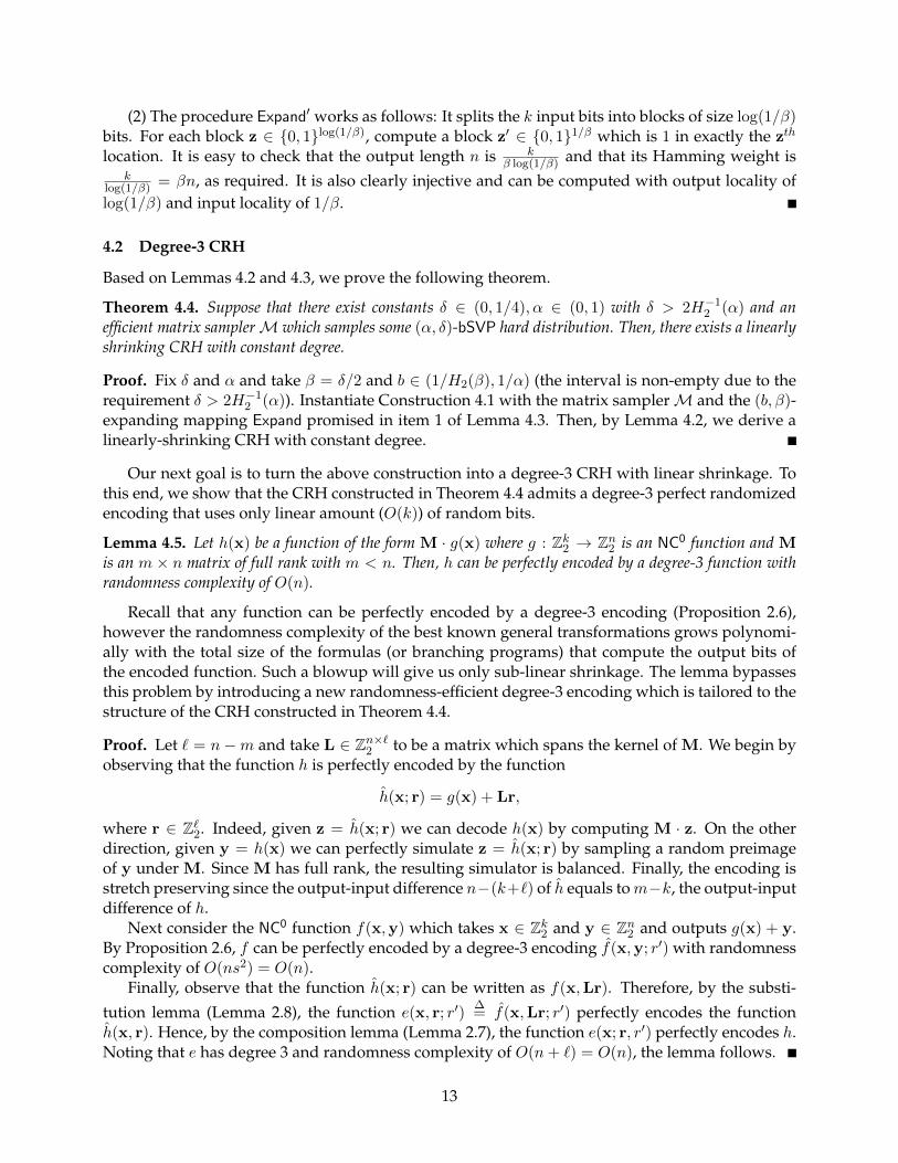
(2) The procedure Expand′ works as follows: It splits the k input bits into blocks of size log(1/β)bits. For each block z ∈ 0, 1log(1/β), compute a block z′ ∈ 0, 11/β which is 1 in exactly the zth

location. It is easy to check that the output length n is kβ log(1/β) and that its Hamming weight is

klog(1/β) = βn, as required. It is also clearly injective and can be computed with output locality oflog(1/β) and input locality of 1/β.

4.2 Degree-3 CRH

Based on Lemmas 4.2 and 4.3, we prove the following theorem.

Theorem 4.4. Suppose that there exist constants δ ∈ (0, 1/4), α ∈ (0, 1) with δ > 2H−12 (α) and an

efficient matrix samplerM which samples some (α, δ)-bSVP hard distribution. Then, there exists a linearlyshrinking CRH with constant degree.

Proof. Fix δ and α and take β = δ/2 and b ∈ (1/H2(β), 1/α) (the interval is non-empty due to therequirement δ > 2H−1

2 (α)). Instantiate Construction 4.1 with the matrix samplerM and the (b, β)-expanding mapping Expand promised in item 1 of Lemma 4.3. Then, by Lemma 4.2, we derive alinearly-shrinking CRH with constant degree.

Our next goal is to turn the above construction into a degree-3 CRH with linear shrinkage. Tothis end, we show that the CRH constructed in Theorem 4.4 admits a degree-3 perfect randomizedencoding that uses only linear amount (O(k)) of random bits.

Lemma 4.5. Let h(x) be a function of the form M · g(x) where g : Zk2 → Zn2 is an NC0 function and Mis an m × n matrix of full rank with m < n. Then, h can be perfectly encoded by a degree-3 function withrandomness complexity of O(n).

Recall that any function can be perfectly encoded by a degree-3 encoding (Proposition 2.6),however the randomness complexity of the best known general transformations grows polynomi-ally with the total size of the formulas (or branching programs) that compute the output bits ofthe encoded function. Such a blowup will give us only sub-linear shrinkage. The lemma bypassesthis problem by introducing a new randomness-efficient degree-3 encoding which is tailored to thestructure of the CRH constructed in Theorem 4.4.

Proof. Let ` = n−m and take L ∈ Zn×`2 to be a matrix which spans the kernel of M. We begin byobserving that the function h is perfectly encoded by the function

h(x; r) = g(x) + Lr,

where r ∈ Z`2. Indeed, given z = h(x; r) we can decode h(x) by computing M · z. On the otherdirection, given y = h(x) we can perfectly simulate z = h(x; r) by sampling a random preimageof y under M. Since M has full rank, the resulting simulator is balanced. Finally, the encoding isstretch preserving since the output-input difference n−(k+`) of h equals tom−k, the output-inputdifference of h.

Next consider the NC0 function f(x,y) which takes x ∈ Zk2 and y ∈ Zn2 and outputs g(x) + y.By Proposition 2.6, f can be perfectly encoded by a degree-3 encoding f(x,y; r′) with randomnesscomplexity of O(ns2) = O(n).

Finally, observe that the function h(x; r) can be written as f(x,Lr). Therefore, by the substi-

tution lemma (Lemma 2.8), the function e(x, r; r′)∆= f(x,Lr; r′) perfectly encodes the function

h(x, r). Hence, by the composition lemma (Lemma 2.7), the function e(x; r, r′) perfectly encodes h.Noting that e has degree 3 and randomness complexity of O(n+ `) = O(n), the lemma follows.

13

Recall that we always assume that a hard-bSVP-distribution puts all but a negligible fraction ofits mass on matrices whose columns are linearly independent. Hence, we can apply Lemma 4.5 tothe CRH constructed in Theorem 4.4, and derive, by Lemma 2.5, the following improved versionof Theorem 4.4.

Theorem 4.6. Under the hypothesis of Theorem 4.4, there exists a linearly shrinking CRH with degree 3.

Instantiating bSVP with the random linear code ensemble, we derive the following corollary.

Corollary 4.7. Suppose that there exist constants δ ∈ (0, 1/4), α ∈ (0, 1) which satisfy δ > 2H−12 (α) for

which (α, δ)− bSVP holds. Then, there exists a degree-3 linearly-shrinking CRH.

Corollary 4.7 serves as a feasibility result for the existence of degree-3 CRH with linear shrink-age. This statement attempts to optimize the parameters of the underlying intractability assump-tion (making it as plausible as possible) and the degree, but yields a poor (constant) shrinkagefactor. By iterating the CRH a sufficiently large (constant) number of times, we can reduce theshrinkage factor to an arbitrary constant ε at the expense of increasing the degree to a large con-stant d = d(ε). Alternatively, we can get a better tradeoff between the degree and the shrinkagefactor by strengthening the assumption as follows.

Proposition 4.8. Suppose that (α, δ)− bSVP holds for every constants δ ∈ (0, 1/4), α ∈ (0, 1) whichsatisfy δ < α/2. Then, for every constants d > 4 and γ > 4/d there exists a degree-d CRH withshrinkage factor of γ.

For example, we can get a degree 5 CRH with shrinkage-factor of 0.81 or degree-8 CRH withshrinkage factor of 0.51.

Proof. Let β = 2−d and recall that item 2 of Lemma 4.3 provides a (b, β)-expanding mappingExpand′ with b = 1

β log(1/β) = 2d/d and output locality (and therefore also degree) of log(1/β) = d.Let δ = 2β = 2−d+1 and α = γ/b. Since γ > 4/d, it follows that δ < α/2, which, according to ourassumption, implies that (α, δ) − bSVP holds. By plugging Expand′ and the matrix-sampler thatsamples uniform αn × n matrices into Construction 4.1, we get, by Lemma 4.2, a degree-d CRHwith shrinkage factor of γ. The proposition follows.

Remark 4.9. Recall that we measure the degree of a collection of functionsH = hz as the maximaldegree of each function in the collection and ignore the degree of the evaluation algorithmH whichmaps the collection key z and the input x to hz(x). (See Remark 2.2.) Nevertheless, it is not hard tosee that all the constructions of this section admit an evaluation algorithm of constant degree. (Infact, the degree is d+ 1 where d is the degree of hz).

4.3 Locally-Computable CRH

Our next goal is to construct CRH’s with constant output and input locality. To this end, we instan-tiate bSVP with the LDPC ensemble.

Theorem 4.10. Suppose that there exist constants δ ∈ (0, 1/4), α ∈ (0, 1) with δ > 2H−12 (α) and a

constant d ∈ N for which (d, α, δ)−bSVP holds. Then, there exists a linearly-shrinking CRH with constantinput locality and constant output locality. Moreover, one can reduce the output locality to 4 (while keepingthe shrinkage linear and the input locality constant).

14

Proof. Fix δ and α and take β = δ/2 and b ∈ (1/H2(β), 1/α). Let Expand be the (b, β)-expandingmapping promised in item 1 of Lemma 4.3 which has input locality of c′ and output locality d′.Instantiate Construction 4.1 with Expand and with the LDPC matrix samplerM which samples auniformly chosen α ·n×nmatrix subject to the constraint that each column contains exactly c = αdones and each row contains exactly d ones. Then, by Lemma 4.2, we derive CRH H = hM withlinear shrinkage, output locality of D = d · d′ and input locality of C = c · c′. This proves the firstpart of the theorem.

For the second part, take the CRH H =hz : 0, 1k → 0, 1m

constructed in the first part

of the theorem, and apply the 4-local perfect encoding promised in Proposition 2.6. The resultingcollection H has the required syntactic properties, and, by Lemma 2.5, it forms a CRH.

Since any NC0 function can be computed by a circuit of linear size, Theorem 4.4 yields a linear-time computable CRH with linear-shrinkage. Such a function can be turned into a linear-timecomputable CRH with arbitrary polynomial-stretch (using a hash-tree), we therefore derive thefollowing corollary.

Corollary 4.11. Under the assumption of Theorem 4.10, for every constant c < 1 there exists a CRHH =

hz : 0, 1k → 0, 1kc

which can be computed by a circuit of size O(k).

5 Degree-2 Hash Functions

In Section 5.1, we construct a universal one-way hash function family under the MQ assumption(see Definition 3.4 for the definition of the Dn,m,p-MQ assumption). We then turn our attention tocollision-resistance. In Section 5.2, we show that a natural family of uniformly random quadraticfunctions is not collision-resistant, by showing an explicit polynomial-time attack. An intriguingquestion left open by our work is the existence of a degree-2 CRH family. In Section 5.3, we showhow this question (and a related question on statistically hiding commitments) relates to a long-standing question on constructing degree-2 randomized encodings.

5.1 Universal One-way Hash Function

Construction 5.1. Let λ be the security parameter, and let n = n(λ), m = m(λ), p = p(λ) (withm < n) be the MQ parameters. Let the MQ distribution D = Dn,m,p be the uniform distributionthat outputs a set of m uniformly random upper-triangular matrices Qi and m vectors Li.

Define the family of hash functionsHn,m,p = h~Q,~L : Znp → Zmp : ~Q ∈ (Zn×np )m, ~L ∈ (Znp )m asfollows:

h~Q,~L(x) =

(xTQix + LTi x

)mi=1

We now show that under the MQ assumption, this family is universal one-way.

Theorem 5.2. Let n = n(λ), m = m(λ), p = p(λ) and Dn,m,p be such that (a) m < n and (b) Dn,m,p isthe uniform distribution. Then, under the Dn,m,p-MQ assumption, the familyHn,m,p is universal one-way.

The construction and proof immediately generalize to other families of distributions where thedistribution of Qi is arbitrary but Li is still uniformly random. In this exposition, we choose topresent the simpler version where both Qi and Li are uniformly random.

Proof. First, since m < n,Hn,m,p is a compressing family of functions.

15

We now show that it is universally one-way. Assume that there is a PPT UOWHF-breakeralgorithm (Adv1,Adv2). We will construct an algorithm B that breaks the D-MQ assumption. Bgets as input an MQ challenge (Qi,Li)

mi=1 and does the following.

• Run Adv1 to get a target input x and state information r.

• Define the UOWHF family using the matrices Q∗i and L∗i where:

Q∗i = Qi and L∗i = Li − (Q∗i + (Q∗i )T )x (5.1)

• Feed ~Q := (Q∗1, . . . ,Q∗m) and ~L := (L∗1, . . . ,L

∗m) to Adv2 together with the state information r.

Get back a colliding input y, output y − x and halt.

First note that the distribution of Qi and Li from equation 5.1 are uniformly random and hence,the adversary Adv = (Adv1,Adv2) will find a colliding input y with non-negligible probability1/q(λ).

Let ∆ := y − x. Since x and y are colliding inputs, we have

(x + ∆)TQ∗i (x + ∆) + (L∗i )T (x + ∆) = xTQ∗ix + (L∗i )

Tx

for all i ∈ [m]. A quick calculation then tells us that

∆TQi∆ + ∆TQix + xTQi∆ + (L∗i )T∆ = ∆TQi∆ +

(xTQT

i + xTQi + (L∗i )T

)∆ = 0

which in turn gives us∆TQi∆ + LTi ∆ = 0 ,

by our definition of Li := L∗i + (Q∗i + (Q∗)T )x. Thus, B outputs a solution to the challenge MQinstance with probability 1/p(λ) as well, which shows that Hn,m,p is a universal one-way hashfamily.

*Generalizing to Other MQ Distributions. Our proof readily generalizes to distributions for theMQ problem which output an arbitrary distribution of the quadratic forms Qi and a uniformlyrandom distribution of the linear forms Li.

*Generalizing to Larger Degrees. Our construction and proof also generalize to the setting wherethe hash function has degree d and can be based on the hardness of solving random degree-dpolynomial equations, a generalization of the MQ assumption. The reason for considering thisgeneralization is to achieve better shrinkage. The MQ construction can shrink n bits to no less thanm =

√n bits, since the MQ assumption is false for smallerm. Since we do not know attacks against

the degree-d assumption with shrinkage m = nΩ(1/d), this variant will give us larger shrinkage atthe expense of larger degree (and a different assumption).

5.2 Finding Collisions in Random Degree-2 Functions

We now show that the hash function family Hn,m,p is not collision-resistant. We remind the readerthatHn,m,p refers to the function where Qi are uniformly random upper-triangular matrices and Liare uniformly random vectors. The attack we describe below was discovered by Ding and Yang [30]but without a proof of correctness.

16

Theorem 5.3. For every n,m < n and p, there is a poly(n,m, log p)-time algorithm ColFinder such that

Prh←Hn,m,p

[ColFinder(h) = (x,y) : h(x) = h(y) ∧ x 6= y] = Ω(1)

In other words, the familyHn,m,p is not collision-resistant.

Proof. The strategy of ColFinder is simple. It chooses a uniformly random ∆ ∈ Znp and solves thesystem of equations

(x + ∆)TQi(x + ∆) + LTi (x + ∆) = xTQix + LTi x

i∈[m]

This is in fact a linear system of equations in the unknown x:Li : xT (QT

i + Qi)∆ + LTi ∆ = 0

i∈[m]

where all computations are done mod p. Any solution x to this system of linear equations gives usa collision (x,x + ∆). Conversely, if there exists a collision with difference ∆, ColFinder will findsuch a collision.

It remains to show that for uniformly random upper-triangular matrices Qi (and possibly uni-formly random ∆ and Li), this system has a solution with high probability. We show a strongerstatement: namely, that the n-by-m matrix Q defined as

Q =

|

... |

(QT1 + Q1)∆

... (QTm + Qm)∆

|... |

has full rank, namely rank m a constant probability. This in turn implies that the equations Li areguaranteed to have a solution with constant probability.

Let us now bound the probability that Q has rank less than m. To do so, let us understand thedistribution of Q using the following observations.

• Fix an i ∈ [m] be such that ∆i 6= 0. Such an i is guaranteed to exist as ∆ 6= 0.

We now claim that for each j ∈ [m], the entries of (Qj + QTj )∆ are uniformly random except

possibly for the i-th entry. This follows from the fact that the i-th column of (Qj + QTj ) is

uniformly random (except for its i-th entry) and uncorrelated to the rest of the matrix exceptthe i-th row (which is identical to the i-th column by symmetry).

• This implies, in turn, that Q has a uniformly random (n−1)-by-m submatrix. The probabilitythat this is full-rank, namely rank min(n− 1,m) = m, is a constant (see, e.g., [17]).

Put together, we see that ColFinder succeeds with constant probability in finding a collision. Weremark that this argument did not use the randomness of Li or ∆, but rather only the fact that theQi are uniformly random upper-triangular matrices.

17

5.3 Degree-2 CRH via Randomized Encoding?

An intriguing question left open by our work is the existence of a degree-2 CRH. The same questionis open also for the related primitive of non-interactive statistically hiding commitments (SHC),which can be easily constructed from a CRH (see Appendix A). We relate these questions to ques-tions about the existence of degree-2 statistically private randomized encodings that were left openby [51].

We start by defining a relaxation of the perfect notion of randomized encoding from Defini-tion 2.4 that allows for statistical privacy error and eliminates the balanced simulation and lengthrequirements.

Definition 5.4 (Statistically-Private, Perfectly Correct Randomized Encoding). Let f : 0, 1n →0, 1m be a function. We say that a function f : 0, 1n × 0, 1ρ → 0, 1s is an ε-private, perfectlycorrect randomized encoding (ε-RE) of f if there exists a deterministic decoding algorithm C and arandomized simulator S which satisfy the following:

• (Perfect correctness.) For every input x ∈ 0, 1n and r ∈ 0, 1ρ, it holds that C(f(x; r))= f(x).

• (ε-privacy) For every x ∈ 0, 1n, the distribution f(x; r), induced by a uniform choice of

rR← 0, 1ρ, satisfies SD(f(x; r), S(f(x))) ≤ ε, where SD denotes statistical distance.

For the dual notion of ε-correct, perfectly-private RE, it is shown in [51] that only very specialfunctions admit such an encoding with a degree-2 f (in the Boolean case, this class of functionsincludes only degree-2 polynomials in the input and functions that test whether the input is in anaffine subspace of 0, 1n). It is open whether the same holds for the above notion of ε-RE.

Question 5.5. Does every finite f : 0, 1n → 0, 1 admit a family of degree-2, εt-private, perfectlycorrect randomized encodings ft : 0, 1n×0, 1ρt → 0, 1st with εt = neg(t) and ρt, st = poly(t)?

This question is open even for the specific function f : 0, 14 → 0, 1 defined byf(a, b, c, d) = abc ⊕ d and even with fixed ε (say ε = 1/3). In fact, it follows from [1] that the latterfunction is complete in the sense that an affirmative answer to Question 5.5 for this function impliesan affirmative answer for all functions.

We show that an affirmative answer to Question 5.5 together with standard cryptographic as-sumptions would imply the existence of a degree-2 SHC. Thus, ruling out such an SHC wouldeffectively require settling Question 5.5 in the negative.

A (non-interactive) SHC is defined by a collection Cz(x, σ), which given a public random stringz (that can be reused for many commitments) maps an input x and secret randomness σ to a com-mitment c. The commitment c should statistically hide x. It should also be computationally bindingin the sense that given z it is infeasible to find a pair (x, σ) and (x′, σ′) which are consistent withthe same c, where x 6= x′. See Appendix A for a formal definition.

Theorem 5.6. Suppose there is a CRH or SHC in NC1. Moreover, suppose that the answer to Question 5.5is affirmative. Then there is a degree-2 SHC.

Proof. Using Theorem A.2, a CRH in NC1 implies an SHC in NC1, which in turn implies an SHCCz(x, σ) in NC0 [1]. Since every output bit of Cz(x, σ) depends on a constant number of input bits,we can apply the degree-2 encoding implied by an affirmative answer to Question 5.5, indepen-dently to every output bit of Cz and with t = |x|, viewing it as a deterministic function of (x, σ).

18

This yields a polynomial-size degree-2 function Cz(x, σ; τ) which is an ε-RE of Cz with ε negligi-ble in k = |x|. We view Cz as a commitment scheme with input x and secret randomness (σ, τ).The perfect correctness requirement of the ε-RE implies that Cz is computationally binding (sinceif (x, (σ, τ)) and (x′, (σ′, τ ′)) violate the binding of Cz then (x, σ) and (x′, σ′) violate the binding ofCz). The statistical hiding property is implied by the fact that the error ε of the ε-RE is negligible inthe input length. Indeed, for every x 6= x′ we have

Cz(x;σ, τ) ≈ Sz(Cz(x;σ)) ≈ Sz(Cz(x′;σ)) ≈ Cz(x′;σ, τ),

where σ, τ are uniformly distributed, ≈ denotes statistical indistinguishability, and Sz is the simu-lator of the encoding.

For the case of CRH, even an affirmative answer to Question 5.5 does not seem to suffice fora degree-2 construction, since an ε-RE of a CRH may lose the shrinking property. Instead, weformulate an ad-hoc variant of randomized encoding that captures a minimal set of requirementsneeded for respecting the CRH properties.

Definition 5.7 (CRH-Respecting Randomized Encoding). Let f : 0, 1n → 0, 1m be a functionwith m < n. We say that a function f : 0, 1n × 0, 1ρ → 0, 1s is a CRH-respecting randomizedencoding of f if the following hold:

• (Perfect correctness.) There exists a deterministic decoding algorithm C such that for everyinput x ∈ 0, 1n and r ∈ 0, 1ρ, it holds that C(f(x; r)) = f(x).

• (Injective randomness) For any fixed x, the function f(x; ·) is injective; namely for any r 6= r′

we have f(x; r) 6= f(x; r′).

• (Shrinkage) The encoding f(x; r) is shrinking, namely s < n+ ρ.

Note that given the perfect correctness and injective randomness requirements, the best onecan hope for is to match the shrinkage of f , namely the shortest possible encoding output is ofsize s = ρ + m. If the shrinkage requirement of Definition 5.7 is strengthened to require this opti-mal shrinkage, the definition becomes equivalent to the notion of PRE from Definition 2.4 [1]. Inparticular, perfect privacy is implied by the perfect correctness, injective randomness, and optimalshrinkage.

On the other hand, even the relaxed requirements of Definition 5.7 do imply some weak form of“average-case privacy.” Indeed, if the input x could always be recovered from f(x, r), then injectiverandomness guarantees that r can also be recovered, and since s < n + ρ we get a contradiction.Thus, the notion of CRH-respecting randomized encoding crudely has the same flavor of perfectcorrectness and partial privacy as the notion of ε-RE from Definition 5.4.

We now show that applying a CRH-respecting randomized encoding to a CRH indeed yields aCRH. (We use concrete function notation instead of infinite collections of functions for simplicity.)

Claim 5.8. Suppose hz : 0, 1n → 0, 1m is a CRH and hz : 0, 1n × 0, 1ρ → 0, 1s is an efficient,CRH-respecting randomized encoding of hz . Then the function hz , viewed as a mapping from n + ρ inputbits to s output bits, is a CRH.

Proof. First, the shrinkage requirement directly guarantees that h is shrinking its input (x, r). Weshow that h inherits the collision resistance of h. Suppose that Adv(z), given a random z, finds acollision (x, r), (x, r′) for hz , where (x, r) 6= (x′, r′). By the injective randomness requirement wemust have x 6= x′ and by perfect correctness we must have h(x) = h(x′). Hence, Adv can be usedto find a collision (x, x′) for h with the same success probability.

19

Finally, we pose a concrete question about the existence of CRH-respecting randomized encod-ings which is related to the existence of degree-2 CRH.

Question 5.9. Does every f : 0, 1n → 0, 1bn/10c in NC0 admit (an efficiently computable)degree-2 CRH-respecting randomized encoding?

Under the assumptions of Theorem 4.10, ruling out a degree-2 CRH would require proving anegative answer to Question 5.9.

6 Win-Win Results

In this section we prove that a failure of our constructions leads to interesting algorithmic conse-quences. Both of our results are based on the following observation.

Lemma 6.1. Suppose that there exists an algorithm Adv with complexity T for which

PrM

R←Zm×n2

[Adv(M) = x such that x 6= 0,Mx = 0 and ∆(x) ≤ δ] ≥ ε.

Then there exists an algorithm Adv′ with complexity T ′ = T + poly(m) such that for every y ∈ Zm2 it holds

PrM

R←Zm×n2

[Adv′(M,y) = x such that Mx = y and ∆(x) ≤ δ] ≥ ε/2.

That is, an algorithm Adv that finds a small subset of the columns of M that spans the all-zerovector, can be transformed into an algorithm Adv′ that finds a small subset of the columns thatspans any given target vector y.

Proof. The algorithm Adv′ is given a random matrix MR← Zm×n2 and an arbitrary target vector

y ∈ Zm2 . It samples a vector u R← Zn2 and calls Adv with the input M′ = M+ y · uT (note that this isan outer-product). Note that if the output x of Adv is (1) a valid solution (i.e., it is a non-zero vectorof weight at most δn and is in the Kernel of M); and (2) is non-orthogonal to u (i.e., 〈x,u〉 = 1),then Mx = Mx + (y · uT )x = y and so Adv′ succeeds.

To analyze the success probability, note that the joint distribution of (M,u) is uniform and there-fore (1) happens with probability ε, by assumption. Moreover, conditioned on (1), the probabilityof (2) is exactly 1

2 . The lemma follows.

6.1 bSVP and Distributed Parity-Learning

In this section we show that if the bSVP assumption (as phrased in Corollary 4.7) does not hold,one can learn parities in a distributed setting with non-trivial memory/communication tradeoffs.The influence of memory and communication restrictions on learning in distributed environmentshas been studied recently by several works (cf. [6, 68, 70, 67] and references therein). We considerhere another variant of this question.

Let us first recall the standard notion of PAC-learning parity functions over uniformly sampledexamples. For a secret parity function fs (s is an m-bit vector), the learner is given random (non-

noisy) labeled samples of the form (ri, bi) where riR← Zm2 is a random example and bi = fs(ri) =

〈ri, s〉 is a binary label. The goal is to predict fs on a random vector r∗ R← Zm2 with probability, say,2/3. We consider the case where the learner is composed of two parties: a measurement device Wthat collects the samples and has only limited memory of S bits and no computational power, and

20

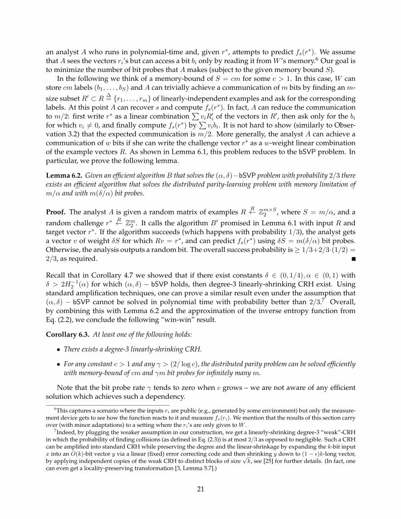
an analyst A who runs in polynomial-time and, given r∗, attempts to predict fs(r∗). We assumethat A sees the vectors ri’s but can access a bit bi only by reading it from W ’s memory.6 Our goal isto minimize the number of bit probes that A makes (subject to the given memory bound S).

In the following we think of a memory-bound of S = cm for some c > 1. In this case, W canstore cm labels (b1, . . . , bS) and A can trivially achieve a communication of m bits by finding an m-

size subset R′ ⊂ R ∆= r1, . . . , rm of linearly-independent examples and ask for the corresponding

labels. At this point A can recover s and compute fs(r∗). In fact, A can reduce the communicationto m/2: first write r∗ as a linear combination

∑viR

′i of the vectors in R′, then ask only for the bi

for which vi 6= 0, and finally compute fs(r∗) by∑vibi. It is not hard to show (similarly to Obser-

vation 3.2) that the expected communication is m/2. More generally, the analyst A can achieve acommunication of w bits if she can write the challenge vector r∗ as a w-weight linear combinationof the example vectors R. As shown in Lemma 6.1, this problem reduces to the bSVP problem. Inparticular, we prove the following lemma.

Lemma 6.2. Given an efficient algorithmB that solves the (α, δ)−bSVP problem with probability 2/3 thereexists an efficient algorithm that solves the distributed parity-learning problem with memory limitation ofm/α and with m(δ/α) bit probes.

Proof. The analyst A is given a random matrix of examples R R← Zm×S2 , where S = m/α, and a

random challenge r∗ R← Zm2 . It calls the algorithm B′ promised in Lemma 6.1 with input R andtarget vector r∗. If the algorithm succeeds (which happens with probability 1/3), the analyst getsa vector v of weight δS for which Rv = r∗, and can predict fs(r∗) using δS = m(δ/α) bit probes.Otherwise, the analysis outputs a random bit. The overall success probability is≥ 1/3+2/3·(1/2) =2/3, as required.

Recall that in Corollary 4.7 we showed that if there exist constants δ ∈ (0, 1/4), α ∈ (0, 1) withδ > 2H−1

2 (α) for which (α, δ) − bSVP holds, then degree-3 linearly-shrinking CRH exist. Usingstandard amplification techniques, one can prove a similar result even under the assumption that(α, δ) − bSVP cannot be solved in polynomial time with probability better than 2/3.7 Overall,by combining this with Lemma 6.2 and the approximation of the inverse entropy function fromEq. (2.2), we conclude the following “win-win” result.

Corollary 6.3. At least one of the following holds:

• There exists a degree-3 linearly-shrinking CRH.

• For any constant c > 1 and any γ > (2/ log c), the distributed parity problem can be solved efficientlywith memory-bound of cm and γm bit probes for infinitely many m.

Note that the bit probe rate γ tends to zero when c grows – we are not aware of any efficientsolution which achieves such a dependency.

6This captures a scenario where the inputs ri are public (e.g., generated by some environment) but only the measure-ment device gets to see how the function reacts to it and measure fs(ri). We mention that the results of this section carryover (with minor adaptations) to a setting where the ri’s are only given to W .

7Indeed, by plugging the weaker assumption in our construction, we get a linearly-shrinking degree-3 “weak”-CRHin which the probability of finding collisions (as defined in Eq. (2.3)) is at most 2/3 as opposed to negligible. Such a CRHcan be amplified into standard CRH while preserving the degree and the linear-shrinkage by expanding the k-bit inputx into an O(k)-bit vector y via a linear (fixed) error correcting code and then shrinking y down to (1 − ε)k-long vector,by applying independent copies of the weak CRH to distinct blocks of size

√k, see [25] for further details. (In fact, one

can even get a locality-preserving transformation [3, Lemma 5.7].)

21

6.2 Speeding-up the BKW algorithm

We move on to the more traditional setting of learning parity with noise (LPN) [18]. Recall that in

this setting the learner is given random noisy labeled samples of the form (ri, bi) where riR← Zm2 is

a random example and bi = fs(ri) +χi is a binary label where fs is a parity function (specified by asecret s ∈ 0, 1m) and χi is a random variable which takes the value 1 with probability τ for somenoise parameter τ ∈ (0, 1

2). The learner should be able to recover s with, say, probability 2/3 whileminimizing the running time and the sample complexity.8

The best known algorithm for solving the LPN problem (i.e., to recover s), due to Blum, Kalaiand Wasserman [19], runs in time (and sample) complexity of 2O(m/ logm). We show that either thecomplexity can be reduced to 2cm/ logm for arbitrary small constant c > 0, or linearly-shrinkingCRH of logarithmic degree exist. To this end, we consider the bSVP assumption (for random linearcodes) in the polynomial regime, i.e., when the number of columns n is polynomially larger thanthe number of rows m.

Assumption 6.4. There exists a positive constant a > 1 for which (α, δ)-bSVP holds for α = 1/n1/a

and δ = 8α/(log(1/α)).

The constant 8 in the above is somewhat arbitrary and any constant larger than 2 suffices. Itwill be useful to state the above assumption in terms of the parameter m (and not n as usual). Thatis, the assumption asserts that, given a random m× (n = ma) binary matrix M, it is hard to find avector of weight w = δn = 8m

(a−1) logm in the kernel of M . Note that, unlike in the previous sections,now the dimensions of the matrix are polynomially related (and not linear) and correspondinglywe can ask for a kernel vector of sub-linear weight.

Lemma 6.5. Suppose that Assumption 6.4 does not hold. Then, for every constant c > 0 and constant noiserate τ ∈ (0, 1

2) there exists an algorithm that for infinitely manym’s, solves them-dimensional LPN problemwith noise rate τ (i.e., recovers the secret s) in time (and sample complexity) of N = poly(m) · 2cm/ logm.

Proof. We describe an algorithm that in time N computes s1, the first bit of s, with probability2/3. Using standard amplification, and by exploiting the symmetry of the LPN problem, suchan algorithm can be converted to an algorithm that recovers s with, say, probability 2/3 at theexpense of increasing the time and sample complexity by a factor of q(m) for some fixed (universal)polynomial q(·). (First reduce the error below 1/3m via repetition and majority vote, and then applythe amplified algorithm m times where in each iteration we recover the i-bit of s by rotating theexamples i− 1 coordinates to the left.)

Let a > 1 be a constant whose value will be determined later, and let w = 8m(a−1) logm . Since

Assumption 6.4 does not hold, there exists, by Lemma 6.1, a polynomial-time algorithm Adva suchthat for infinitely many m’s, for all y ∈ Zm2

PrM

R←Zm×ma2

[Adva(M,y) = x such that Mx = y and x has Hamming weight of at most w],

is larger than some inverse polynomial ε(m).Let n = ma, µ = 1 − 2τ , t = O(µ2w) and t′ = O(t/ε). The algorithm asks for nt′ labeled

examples and partitions them into t′ sets Ti each of n examples. For each set Ti, let Si denote theset of examples without their noisy labels. We apply Adva to Si and set the target vector y to be

8Again, we could define the goal as predicting the value fs(r∗) for random r∗ with non-trivial success probability.However, in this setting the two goals reduces to each other with polynomial overhead.

22

the first unit vector e1. If Adva succeeds (i.e., returns a subset S′i ⊆ Si of size bmlogm whose sum is

e1) then we XOR together the labels that correspond to the vectors in S′i and record the result as avote vj (which serves as a guess for s1). If the algorithm fails, we do not record the vote. Finally,we output the majority of all recorded votes vj .

Analysis: First we claim that each recorded vote is correct (equals to s1) independently withprobability 1/2 + µw. Indeed, each vote is of the form s1 +

∑wi=1 χi where the χi’s are independent

Bernoulli variables each with expectation τ . It is well known (e.g., [19, Lemma 4]) that χ =∑w

i=1 χiis a Bernoulli random variable with expectation of (1− µw)/2 for µ = 1− 2τ .

Next, we argue that, except with probability 1/10, there is a large number of votes. Indeed,each invocation of Adva succeeds with at least ε probability hence, by Markov’s inequality, theprobability that there are less than t successful invocations out of, say t′ = 10t/ε attempts, is atmost 1/10.

Finally, conditioned on having t votes, by a Chernoff bound, the probability that the final out-come is wrong is 1/10. The claim follows by a union bound.

Overall, the time complexity of the algorithm is

O(nt′) = O(ma · (1− 2τ)20m

(a−1) logm ) = O(ma · e8m

τ(a−1) logm ),

where e is the natural exponent. Hence, we get the desired running time by taking a = a(τ, c) to bea sufficiently large constant.

Next we show that if Assumption 6.4 holds then we get CRH of logarithmic degree.

Lemma 6.6. Under Assumption 6.4, there exists a linearly-shrinking CRH with logarithmic degree.

Proof. Let a > 1 be the constant promised by Assumption 6.4 and let α = 1n1/a , δ = 8α

log(1/α) . Also,let

d = log(2/δ) = log(n1/a) + log log(n1/a)− 2, β = 2−d,

b =2d

d=

n1/a log(n1/a)

4(log(n1/a) + log log(n1/a)− 2).

We instantiate Construction 4.1 with the (α, δ)-bSVP sampler and with the (b, β)-expanding map-ping promised in the second item of Lemma 4.3. (This part of the lemma holds for non-constant βas well.) Since β ≤ δ/2 and bα < 1/4, we get, by Lemma 4.2, a linearly shrinking CRH with degreeof d = O(log n). The lemma follows.

We conclude the following corollary.

Corollary 6.7. At least one of the following holds:

• There exists a linearly-shrinking CRH with logarithmic degree.

• For any constant c > 0 and any constant noise rate τ ∈ (0, 12) there exists an algorithm that, for

infinitely many m, solves the m-dimensional LPN problem with noise rate τ in time and samplecomplexity of poly(m) · 2cm/ logm.

23

7 Conclusions and Open Questions

Under plausible intractability assumptions, we establish the existence of low-complexity crypto-graphic hash functions that compress the input by (at least) a constant factor. In particular, weconstruct CRH with linear circuit size, constant locality, or algebraic degree 3 over Z2 under differ-ent flavors of the newly introduced binary SVP (bSVP) assumption. We also establish connectionswith other problems that either support our assumptions or indicate that further progress may bedifficult.

While we provide some evidence supporting the validity of the flavors of bSVP we rely on,including a weak connection with the LPN problem, it is left open to obtain a better understandingof the relation between bSVP and LPN or other well studied cryptographic assumptions. It wouldalso be interesting to obtain similar positive results under better or incomparable assumptions,such as the MQ assumption (that we use to construct degree-2 UOWHFs) or the one-wayness ofrandom local functions (used in [3] for constructing local UOWHFs).

Our work leaves open several other natural questions. One such question is the existence ofCRH (or even 2-message statistically hiding commitments) with degree 2 or output locality 3. An-other is the maximal achievable compression of a degree-d CRH: The bSVP-based security analysisof our construction can only support a constant compression factor, which seems unlikely to beoptimal. (In contrast, for linear-size CRH we can provide an arbitrary polynomial compression.)A final question is to understand the collision resistance properties of random degree-d mappings.While we rule out collision resistance for d = 2 with any non-trivial compression, the question iswide open for d ≥ 3. It would be interesting to study the maximal compression (if any) for whicha random degree-d mapping can be a CRH.

Acknowledgement

We thank Zvika Brakerski for participating in an earlier stage of this project. We also thank DavidBurstein, Simon Litsyn, Ronny Roth, Ohad Shamir, and David Woodruff for helpful discussions.

This work was done in part while the authors were visiting the Simons Institute for the Theoryof Computing, supported by the Simons Foundation and by the DIMACS/Simons Collaborationin Cryptography through NSF grant CNS-1523467. The first author was partially supported bythe European Union’s Horizon 2020 Programme (ERC-StG-2014-2020) under grant agreement no.639813 ERC-CLC, by an ICRC grant and by the Check Point Institute for Information Security.The second author was partially supported by a Melvin R. Berlin Fellowship in the Cyber Secu-rity Research Program. The second and third authors were partially supported by ERC startinggrant 259426. The second, third and fourth authors were partially supported by ISF grant 1709/14,BSF grant 2012378, and NSF-BSF grant 2015782. The third author was additionally supported bya DARPA/ARL SAFEWARE award, NSF Frontier Award 1413955, NSF grants 1228984, 1136174,1118096, and 1065276, and DARPA through the ARL under Contract W911NF-15-C-0205. The fifthauthor was partially supported by NSF Grants CNS-1350619 and CNS-1414119, Alfred P. Sloan Re-search Fellowship, Microsoft Faculty Fellowship, the NEC Corporation, a Steven and Renee FinnCareer Development Chair from MIT, and DARPA and U.S. Army Research Office under contractsW911NF-15-C-0226. The views expressed are those of the authors and do not reflect the officialpolicy or position of the Department of Defense, the National Science Foundation, or the U.S. Gov-ernment.

24

References

[1] Benny Applebaum, Yuval Ishai, and Eyal Kushilevitz. Cryptography in NC0. SIAM J. Comput.,36(4):845–888, 2006.

[2] Benny Applebaum, Yuval Ishai, and Eyal Kushilevitz. How to garble arithmetic circuits. SIAMJ. Comput., 43(2):905–929, 2014.

[3] Benny Applebaum and Yoni Moses. Locally computable UOWHF with linear shrinkage. InAdvances in Cryptology - EUROCRYPT 2013, 32nd Annual International Conference on the Theoryand Applications of Cryptographic Techniques, Athens, Greece, May 26-30, 2013. Proceedings, pages486–502, 2013.

[4] Daniel Augot, Matthieu Finiasz, and Nicolas Sendrier. A family of fast syndrome based cryp-tographic hash functions. In Progress in Cryptology - Mycrypt 2005, First International Conferenceon Cryptology in Malaysia, Kuala Lumpur, Malaysia, September 28-30, 2005, Proceedings, pages64–83, 2005.

[5] Jean-Philippe Aumasson and Willi Meier. Analysis of Multivariate Hash Functions. In Infor-mation Security and Cryptology - ICISC 2007, 10th International Conference, Seoul, Korea, November29-30, 2007, Proceedings, pages 309–323, 2007.

[6] Maria-Florina Balcan, Avrim Blum, Shai Fine, and Yishay Mansour. Distributed learning,communication complexity and privacy. In COLT 2012 - The 25th Annual Conference on LearningTheory, June 25-27, 2012, Edinburgh, Scotland, pages 26.1–26.22, 2012.

[7] Boaz Barak. How to go beyond the black-box simulation barrier. In 42nd Annual Symposium onFoundations of Computer Science, FOCS 2001, 14-17 October 2001, Las Vegas, Nevada, USA, pages106–115, 2001.

[8] Alexander Barg. Complexity issues in coding theory. Electronic Colloquium on ComputationalComplexity (ECCC), 4(46), 1997.

[9] Alexander Barg and G. David Forney Jr. Random codes: Minimum distances and error expo-nents. IEEE Trans. Information Theory, 48(9):2568–2573, 2002.

[10] Anja Becker, Antoine Joux, Alexander May, and Alexander Meurer. Decoding random binarylinear codes in 2 n/20: How 1 + 1 = 0 improves information set decoding. In Advances in Cryp-tology - EUROCRYPT 2012 - 31st Annual International Conference on the Theory and Applicationsof Cryptographic Techniques, Cambridge, UK, April 15-19, 2012. Proceedings, pages 520–536, 2012.

[11] Mihir Bellare and Phillip Rogaway. Collision-resistant hashing: Towards making uowhfs prac-tical. In Advances in Cryptology - CRYPTO ’97, 17th Annual International Cryptology Conference,Santa Barbara, California, USA, August 17-21, 1997, Proceedings, pages 470–484, 1997.

[12] Michael Ben-Or, Shafi Goldwasser, and Avi Wigderson. Completeness theorems for non-cryptographic fault-tolerant distributed computation (extended abstract). In Proceedings ofthe 20th Annual ACM Symposium on Theory of Computing, May 2-4, 1988, Chicago, Illinois, USA,pages 1–10, 1988.

[13] Come Berbain, Henri Gilbert, and Jacques Patarin. QUAD: A multivariate stream cipher withprovable security. J. Symb. Comput., 44(12):1703–1723, 2009.

25

[14] Daniel J. Bernstein, Tanja Lange, and Christiane Peters. Smaller decoding exponents: Ball-collision decoding. In Advances in Cryptology - CRYPTO 2011 - 31st Annual Cryptology Confer-ence, Santa Barbara, CA, USA, August 14-18, 2011. Proceedings, pages 743–760, 2011.

[15] Olivier Billet, Matthew J. B. Robshaw, and Thomas Peyrin. On Building Hash Functions fromMultivariate Quadratic Equations. In Information Security and Privacy, 12th Australasian Con-ference, ACISP 2007, Townsville, Australia, July 2-4, 2007, Proceedings, pages 82–95, 2007.

[16] Nir Bitansky, Ran Canetti, Alessandro Chiesa, Shafi Goldwasser, Huijia Lin, Aviad Rubinstein,and Eran Tromer. The hunting of the SNARK. IACR Cryptology ePrint Archive, 2014:580, 2014.

[17] Johannes Blomer, Richard Karp, and Emo Welzl. The rank of sparse random matrices overfinite fields. Random Struct. Algorithms, 10(4):407–419, 1997.

[18] Avrim Blum, Merrick L. Furst, Michael J. Kearns, and Richard J. Lipton. Cryptographic prim-itives based on hard learning problems. In Advances in Cryptology - CRYPTO ’93, 13th AnnualInternational Cryptology Conference, Santa Barbara, California, USA, August 22-26, 1993, Proceed-ings, pages 278–291, 1993.

[19] Avrim Blum, Adam Kalai, and Hal Wasserman. Noise-tolerant learning, the parity problem,and the statistical query model. In Proceedings of the Thirty-Second Annual ACM Symposium onTheory of Computing, May 21-23, 2000, Portland, OR, USA, pages 435–440, 2000.

[20] Manuel Blum and Silvio Micali. How to generate cryptographically strong sequences ofpseudo random bits. In 23rd Annual Symposium on Foundations of Computer Science, Chicago,Illinois, USA, 3-5 November 1982, pages 112–117, 1982.

[21] Elette Boyle, Niv Gilboa, and Yuval Ishai. Breaking the circuit size barrier for secure com-putation under DDH. In Advances in Cryptology - CRYPTO 2016 - 36th Annual InternationalCryptology Conference, Santa Barbara, CA, USA, August 14-18, 2016, Proceedings, Part I, pages509–539, 2016.

[22] Zvika Brakerski and Vinod Vaikuntanathan. Efficient fully homomorphic encryption from(standard) LWE. SIAM J. Comput., 43(2):831–871, 2014.

[23] David Burshtein and Gadi Miller. Bounds on the performance of belief propagation decoding.IEEE Trans. Information Theory, 48(1):112–122, 2002.

[24] Chris Calabro. The Exponential Complexity of Satisfiability Problems. PhD thesis, University ofCalifornia, San Diego, 2009.

[25] Ran Canetti, Ronald L. Rivest, Madhu Sudan, Luca Trevisan, Salil P. Vadhan, and HoeteckWee. Amplifying collision resistance: A complexity-theoretic treatment. In Advances in Cryp-tology - CRYPTO 2007, 27th Annual International Cryptology Conference, Santa Barbara, CA, USA,August 19-23, 2007, Proceedings, pages 264–283, 2007.

[26] David Chaum, Claude Crepeau, and Ivan Damgard. Multiparty unconditionally secure pro-tocols (extended abstract). In Proceedings of the 20th Annual ACM Symposium on Theory of Com-puting, May 2-4, 1988, Chicago, Illinois, USA, pages 11–19, 1988.

[27] Ronald Cramer, Ivan Damgard, and Ueli M. Maurer. General secure multi-party computationfrom any linear secret-sharing scheme. In Advances in Cryptology - EUROCRYPT 2000, Interna-tional Conference on the Theory and Application of Cryptographic Techniques, Bruges, Belgium, May14-18, 2000, Proceeding, pages 316–334, 2000.

26

[28] Ivan Damgard. Collision Free Hash Functions and Public Key Signature Schemes. In Advancesin Cryptology - EUROCRYPT ’87, Workshop on the Theory and Application of of CryptographicTechniques, Amsterdam, The Netherlands, April 13-15, 1987, Proceedings, pages 203–216, 1987.

[29] Ivan Damgard, Torben P. Pedersen, and Birgit Pfitzmann. On the existence of statisticallyhiding bit commitment schemes and fail-stop signatures. J. Cryptology, 10(3):163–194, 1997.

[30] Jintai Ding and Bo-Yin Yang. Multivariates polynomials for hashing. In Information Securityand Cryptology, Third SKLOIS Conference, Inscrypt 2007, Xining, China, August 31 - September 5,2007, Revised Selected Papers, pages 358–371, 2007.

[31] Ilya Dumer. On minimum distance decoding of linear codes. In Ed. G. Kabatianskii, editor,Fifth Soviet-Swedish intern. workshop Information theory, pages 50–52, 1991.

[32] Ilya Dumer, Alexey A Kovalev, and Leonid P Pryadko. Distance verification for LDPC codes.arXiv preprint arXiv:1605.02410, 2016.

[33] Ilya Dumer, Daniele Micciancio, and Madhu Sudan. Hardness of approximating the minimumdistance of a linear code. IEEE Trans. Information Theory, 49(1):22–37, 2003.

[34] Uriel Feige, Jeong Han Kim, and Eran Ofek. Witnesses for non-satisfiability of dense random3cnf formulas. In 47th Annual IEEE Symposium on Foundations of Computer Science (FOCS 2006),21-24 October 2006, Berkeley, California, USA, Proceedings, pages 497–508, 2006.

[35] Matthieu Finiasz, Philippe Gaborit, and Nicolas Sendrier. Improved fast syndrome basedcryptographic hash functions. In Proceedings of ECRYPT Hash Workshop, volume 2007, page155, 2007.

[36] Matthieu Finiasz and Nicolas Sendrier. Security bounds for the design of code-based cryp-tosystems. In Advances in Cryptology - ASIACRYPT 2009, 15th International Conference on theTheory and Application of Cryptology and Information Security, Tokyo, Japan, December 6-10, 2009.Proceedings, pages 88–105, 2009.

[37] Robert G. Gallager. Low-Density Parity-Check Codes. 1963.

[38] M. R. Garey and David S. Johnson. Computers and Intractability: A Guide to the Theory of NP-Completeness. 1979.

[39] Craig Gentry. Fully homomorphic encryption using ideal lattices. In Proceedings of the 41stAnnual ACM Symposium on Theory of Computing, STOC 2009, Bethesda, MD, USA, May 31 - June2, 2009, pages 169–178, 2009.

[40] Craig Gentry, Amit Sahai, and Brent Waters. Homomorphic encryption from learning witherrors: Conceptually-simpler, asymptotically-faster, attribute-based. In Advances in Cryptology- CRYPTO 2013 - 33rd Annual Cryptology Conference, Santa Barbara, CA, USA, August 18-22,2013. Proceedings, Part I, pages 75–92, 2013.

[41] Oded Goldreich. Candidate One-Way Functions Based on Expander Graphs. In Studies inComplexity and Cryptography. Miscellanea on the Interplay between Randomness and Computation- In Collaboration with Lidor Avigad, Mihir Bellare, Zvika Brakerski, Shafi Goldwasser, Shai Halevi,Tali Kaufman, Leonid Levin, Noam Nisan, Dana Ron, Madhu Sudan, Luca Trevisan, Salil Vadhan,Avi Wigderson, David Zuckerman, pages 76–87. 2011.

27

[42] Oded Goldreich, Shafi Goldwasser, and Shai Halevi. Collision-free hashing from lattice prob-lems. Electronic Colloquium on Computational Complexity (ECCC), 3(42), 1996.

[43] Oded Goldreich, Shafi Goldwasser, and Silvio Micali. How to construct random functions.Journal of the ACM, 33(4):792–807, 1986.

[44] Venkatesan Guruswami, Atri Rudra, and Madhu Sudan. Essential coding theory. Draft of aBook, 2015.

[45] Iftach Haitner, Jonathan J. Hoch, Omer Reingold, and Gil Segev. Finding collisions in in-teractive protocols - tight lower bounds on the round and communication complexities ofstatistically hiding commitments. SIAM J. Comput., 44(1):193–242, 2015.

[46] Iftach Haitner, Yuval Ishai, Eran Omri, and Ronen Shaltiel. Parallel hashing via list recover-ability. In Advances in Cryptology - CRYPTO 2015 - 35th Annual Cryptology Conference, SantaBarbara, CA, USA, August 16-20, 2015, Proceedings, Part II, pages 173–190, 2015.

[47] Shai Halevi and Silvio Micali. Practical and provably-secure commitment schemes fromcollision-free hashing. In Advances in Cryptology - CRYPTO ’96, 16th Annual International Cryp-tology Conference, Santa Barbara, California, USA, August 18-22, 1996, Proceedings, pages 201–215,1996.

[48] Masanori Hirotomo, Masami Mohri, and Masakatu Morii. A probabilistic computationmethod for the weight distribution of low-density parity-check codes. In Proceedings. Inter-national Symposium on Information Theory, 2005. ISIT 2005., pages 2166–2170, 2005.

[49] Chun-Yuan Hsiao and Leonid Reyzin. Finding collisions on a public road, or do secure hashfunctions need secret coins? In Advances in Cryptology - CRYPTO 2004, 24th Annual Inter-national CryptologyConference, Santa Barbara, California, USA, August 15-19, 2004, Proceedings,pages 92–105, 2004.

[50] Xiao-Yu Hu, Marc P. C. Fossorier, and Evangelos Eleftheriou. On the computation of the mini-mum distance of low-density parity-check codes. In Proceedings of IEEE International Conferenceon Communications, ICC 2004, Paris, France, 20-24 June 2004, pages 767–771, 2004.

[51] Yuval Ishai and Eyal Kushilevitz. Randomizing polynomials: A new representation withapplications to round-efficient secure computation. In 41st Annual Symposium on Foundationsof Computer Science, FOCS 2000, 12-14 November 2000, Redondo Beach, California, USA, pages294–304, 2000.

[52] Yuval Ishai, Eyal Kushilevitz, Rafail Ostrovsky, and Amit Sahai. Cryptography with constantcomputational overhead. In Proceedings of the 40th Annual ACM Symposium on Theory of Com-puting, Victoria, British Columbia, Canada, May 17-20, 2008, pages 433–442, 2008.

[53] Ahmet B. Keha and Tolga M. Duman. Minimum distance computation of LDPC codes usinga branch and cut algorithm. IEEE Trans. Communications, 58(4):1072–1079, 2010.

[54] Joe Kilian. A note on efficient zero-knowledge proofs and arguments (extended abstract). InProceedings of the 24th Annual ACM Symposium on Theory of Computing, May 4-6, 1992, Victoria,British Columbia, Canada, pages 723–732, 1992.

28

[55] Aviad Kipnis, Jacques Patarin, and Louis Goubin. Unbalanced Oil and Vinegar SignatureSchemes. In Advances in Cryptology - EUROCRYPT ’99, International Conference on the Theoryand Application of Cryptographic Techniques, Prague, Czech Republic, May 2-6, 1999, Proceeding,pages 206–222, 1999.

[56] Aviad Kipnis and Adi Shamir. Cryptanalysis of the HFE public key cryptosystem by relin-earization. In Advances in Cryptology - CRYPTO ’99, 19th Annual International Cryptology Con-ference, Santa Barbara, California, USA, August 15-19, 1999, Proceedings, pages 19–30, 1999.

[57] Simon Litsyn and Vladimir Shevelev. On ensembles of low-density parity-check codes:asymptotic distance distributions. IEEE Transactions on Information Theory, 48(4):887–908, 2002.

[58] Vadim Lyubashevsky and Daniele Micciancio. Generalized compact knapsacks are collisionresistant. In Automata, Languages and Programming, 33rd International Colloquium, ICALP 2006,Venice, Italy, July 10-14, 2006, Proceedings, Part II, pages 144–155, 2006.

[59] Tsutomu Matsumoto and Hideki Imai. Public Quadratic Polynominal-Tuples for EfficientSignature-Verification and Message-Encryption. In Advances in Cryptology - EUROCRYPT ’88,Workshop on the Theory and Application of of Cryptographic Techniques, Davos, Switzerland, May25-27, 1988, Proceedings, pages 419–453, 1988.

[60] Ralph C. Merkle. A digital signature based on a conventional encryption function. In Ad-vances in Cryptology - CRYPTO ’87, A Conference on the Theory and Applications of CryptographicTechniques, Santa Barbara, California, USA, August 16-20, 1987, Proceedings, pages 369–378, 1987.

[61] Ralph C. Merkle. A Certified Digital Signature. In Advances in Cryptology - CRYPTO ’89, 9thAnnual International Cryptology Conference, Santa Barbara, California, USA, August 20-24, 1989,Proceedings, pages 218–238, 1989.

[62] Silvio Micali. Computationally sound proofs. SIAM Journal on Computing, 30(4):1253–1298,2000. Preliminary version in FOCS’94.

[63] Moni Naor and Moti Yung. Universal one-way hash functions and their cryptographic appli-cations. In Proceedings of the 21st Annual ACM Symposium on Theory of Computing, May 14-17,1989, Seattle, Washigton, USA, pages 33–43, 1989.

[64] Jacques Patarin. Cryptoanalysis of the Matsumoto and Imai Public Key Scheme of Euro-crypt’88. In Advances in Cryptology - CRYPTO ’95, 15th Annual International Cryptology Con-ference, Santa Barbara, California, USA, August 27-31, 1995, Proceedings, pages 248–261, 1995.

[65] Chris Peikert and Alon Rosen. Efficient collision-resistant hashing from worst-case assump-tions on cyclic lattices. In Theory of Cryptography, Third Theory of Cryptography Conference, TCC2006, New York, NY, USA, March 4-7, 2006, Proceedings, pages 145–166, 2006.

[66] Tal Rabin and Michael Ben-Or. Verifiable secret sharing and multiparty protocols with honestmajority (extended abstract). In Proceedings of the 21st Annual ACM Symposium on Theory ofComputing, May 14-17, 1989, Seattle, Washigton, USA, pages 73–85, 1989.

[67] Ran Raz. Fast learning requires good memory: A time-space lower bound for parity learning.Electronic Colloquium on Computational Complexity (ECCC), 23:19, 2016.

29

[68] Ohad Shamir. Fundamental limits of online and distributed algorithms for statistical learningand estimation. In Advances in Neural Information Processing Systems 27: Annual Conference onNeural Information Processing Systems 2014, December 8-13 2014, Montreal, Quebec, Canada, pages163–171, 2014.

[69] Daniel R. Simon. Finding collisions on a one-way street: Can secure hash functions be basedon general assumptions? In Advances in Cryptology - EUROCRYPT ’98, International Conferenceon the Theory and Application of Cryptographic Techniques, Espoo, Finland, May 31 - June 4, 1998,Proceeding, pages 334–345, 1998.

[70] Jacob Steinhardt, Gregory Valiant, and Stefan Wager. Memory, communication, and statisticalqueries. In Proceedings of the 29th Conference on Learning Theory, COLT 2016, New York, USA,June 23-26, 2016, pages 1490–1516, 2016.

[71] Jacques Stern. A method for finding codewords of small weight. In Coding Theory and Ap-plications, 3rd International Colloquium, Toulon, France, November 2-4, 1988, Proceedings, pages106–113, 1988.

[72] Alexander Vardy. The intractability of computing the minimum distance of a code. IEEE Trans.Information Theory, 43(6):1757–1766, 1997.

[73] Christopher Wolf. Multivariate quadratic polynomials in public key cryptography. Cryptol-ogy ePrint Archive, Report 2005/393, 2005.

[74] Yang Xiao and Kiseon Kim. Searching the minimum distances of LDPC codes. In Wireless,Mobile and Multimedia Networks (ICWMMN 2008), IET 2nd International Conference on, pages211–214, 2008.

[75] Andrew Chi-Chih Yao. Theory and applications of trapdoor functions (extended abstract). In23rd Annual Symposium on Foundations of Computer Science, Chicago, Illinois, USA, 3-5 November1982, pages 80–91, 1982.

A Statistically Hiding Commitments

In this section we define a non-interactive notion of statistically hiding commitments (SHC), whichcan be viewed as a randomized version of CRH that achieves an input hiding property. We thenshow that positive results for CRH apply also to the case of SHC.

Similarly to a CRH, an SHC is defined by a public random string z (which can be reused formany commitments). The string z defines a mapping from an input x and secret randomness σ toa commitment string c. The commitment c should statistically hide x. It should also be computa-tionally binding in the sense that given z it is infeasible to find a pair (x, σ) and (x′, σ′) which areconsistent with the same c, where x 6= x′. We formalize these requirements below.

Definition A.1 (Statistically Hiding Commitment). A collection of functions

C =Cz : 0, 1k × 0, 1ρ(k) → 0, 1m(k)

z∈0,1s(k)

is a (non-interactive) statistically hiding commitment (SHC) if the following hold:

• (Efficient evaluation and sampling) There exists a pair of efficient algorithms: (a) a commit-ment algorithm C which given (z ∈ 0, 1s, x ∈ 0, 1k, σ ∈ 0, 1ρ) outputs Cz(x, σ); and (b) akey-sampling algorithm K which given 1k samples a index z ∈ 0, 1s(z).

30

• (Statistical hiding) For every pair of inputs x, x′ ∈ 0, 1k we have

SD((z, Cz(x, σ)), (z, Cz(x′, σ))) ≤ neg(k),

where SD denotes statistical distance, z is picked by K(1k), and σ is picked uniformly from0, 1ρ(k).

• (Computational binding) For every probabilistic polynomial-time adversary Adv itholds that

PrzR←K(1k)

[Adv(z) = ((x, σ), (x′, σ′)) s.t. x′ 6= x and Cz(x, σ) = Cz(x′, σ′)] ≤ neg(k).

As in the case of CRH, we consider the efficiency of SHC for any fixed public challenge z,namely z defines a function of x and s. This is justified by the fact that the same z can reused.

We now show a simple transformation of a CRH into an SHC using a randomness extractor [29,47]. The high level idea is to apply a CRH to a secret random input α, and then mask the SHC inputwith randomness extracted from α. Since the CRH shrinks the input, there is residual entropy in αeven when conditioned on the output of the CRH.

Theorem A.2. Suppose H =hz : 0, 1k → 0, 1m(k)

z∈0,1s(k) is a CRH, where m(k) = b(1− c)kc

for some constant 0 < c < 1. Let Extk : 0, 1k × 0, 1d → 0, 1bck/3c be a strong (ck/2, ε) randomnessextractor with error ε(k) = neg(k).Then C =

Cz : 0, 1k′ × 0, 1k+d → 0, 1m(k)

z∈0,1s(k)

, where k(k′) is chosen such that bck/3c =

k′ and Cz(x′, (α, β)) = (hz(α), β, x′ ⊕ Extk(α, β)) for α ∈ 0, 1k and β ∈ 0, 1d, is an SHC.

Implementing Ext by a random linear function, the SHC obtained in Theorem A.2 has the samealgebraic degree as the underlying CRH. Moreover, if Ext is implemented by the linear-size pair-wise independent hash function from [52], the SHC additionally maintains the asymptotic circuitsize of the CRH. Thus, we get a linear-size (degree-3) SHC under the assumptions of Theorem 4.10.

Unlike the case of CRH, there is no shrinkage requirement for SHC, hence a degree-3 SHCwith locality 4 is implied by the existence of any SHC or CRH in NC1, which is in turn impliedby most standard cryptographic assumptions [1]. However, the existence of degree-2 SHC is leftopen. Using Theorem A.2, a degree-2 SHC would be implied by the existence of a degree-2 CRH,which is one of the main questions left open by this work.

31