•

•

•

•

LOST CALL CLEARED SYSTEMS WITH UNBALANCED TRAFFIC SOURCES

J. P. Dartois

Compagnie Generale de Constructions Telephoniques, associated with ITT

Paris, France

SUMMARY

The main purpose of this study is to thro .... more light on the economical And practical aspects of the problem of unbalanced traffic sources connected to lost call cleared systems. The numerical study is performed on some typical examples of one-stage-full-availability groups and link systems with concentration in the first s .... itching stage; most of the results can be considered as general ones for these configurations. The possible advantages of consid­ering unbalanced sources instead of identical ones are demonstrated and numerically evaluated in terms of gains in traffic capacity. Practical traffic engineering curves are proposed, illustrating the variations of these gains versus the characteristic parameter of the traffic unbal­ance.

The problem of establishing a realistic dimensioning cri­terium is discussed and solutions are proposed.

The theoretical part of the study consists in a presenta­tion of a general mathematical model for lost-call-cleared systems. This model covers all possible traffic source configurations, .... ith or without unbalance. For practical telephone applications, this model is particularized for the one-stage full availability groups and the state prob­ability distribution in the stationary state is given .... ith the most general formulation.

ACKNOWLEDGEMENTS

The author wishes to express his thanks to Mr. A.R. RODRIGUEZ, head of the Traffic Division of the ITT Laboratories of Spain (Madrid) and to Messrs. J.E. VILLAR and M. GARCIA CORDERO of ITTLS for their help in writing the traffic simulation program used for t~e link systems considered in this report •

215/1

I. INTRODUCTION

The problem of unbalanced traffic sources can be analyzed and developed from two complementary approaches. In the first one, presented in [1] , small groups of randoMly cho-sen traffic sources .... ere studied. The possible dangers of su::h a randomchoice .... ere stressed through the fact that the traffic of the group may exceed a certain given maximum value, leading to possibilities of large congestion values in the loss-system to .... hich the group under consideration is connected.

In the second approach, .... hich constitutes the Object of the present study, small groups of selectively chosen sources are considered; this selective choice is made according to the individual traffic of each source, .... hich is assumed to be a-priori kno .... n. These unbalanced groups are connected to lost call-cleared systems and the result­ing congestions are studied on both numerical and theoret­ical aspects.

The numerical study is performed on some typical examples of one-stage-full-availability groups and link-systems .... ith concentration in the first s .... itching stage; most of the results can be considered as general ones for these configurations.

A theoretical mathematical model is developed in the ap­pendix, covering all possible traffic source configura­tions. The use of the Markov process theory allo .... s obtain­ing explicit formulae for the state probability distrib­ution in the stationary state. For telephone applications, this model is particularized for the one-stage-full avail­ability groups for .... hich the state-probability distribu­tion is given in the most general .... ay. According to each specific example of unbalanced s,ource configuration, it is then possible to derive the exact formulae for the congestions in terms of the state probabilities and, fur­ther, to compute them.

11. ONE STAGE FULL-AVAILABILITY GROUPS WITH UNBALANCED TRAFFIC SOURCES

11.1. Statement of the problem

One stage full-availability groups are considered here; they are characterized by their number R (finite) of de­vices and their total number K of traffic sources (K> R and K finite or not). These groups .... ork under the "lost-call-cleared" assumptions. The objectives are to establish the expressions of the occupancy probability distributions and to derive the blocking formulae under the follo .... ing alternative conditions :

either the K sources are strictly identical, .... ith an of­fered traffic 6(; per source

or, reversely, the K sources are not identical, insofar as their traffic characteristics are concerned.

The first case leads to the very .... ell-kno .... n "Engset" or "Erlang" occupancy probabili ty distributions, . according to .... hether K> R or K • R. In the Engset case, the call and time congestions are respectively denoted C* and B* and, further on, many references will be made to these co~gestions.

For non-identical traffic sources, the most general case is obtained when considering n homogeneous groups of sources G , ••• , G , with each G. characterized by the following 1 paramete¥s : ~

* K .. the number of strictly identical sources composing tFte group

* ~. the offered traffic per source or

1A. the total . offered traffic of the group

* h . tFte mathematical expectation of the source occupa­tion holding time distribution

* the mathematical traffic model of emission of calls, which is either an "Engset process" or an "Erlang proc­ess", truncated or not.

Formulae are found in the Appendix, explicitly giving the state probability distribution for this general case.

For practical applications, this general case is mainly particularized in the case of n = 2 homogeneous groups of sources, representing either 2 groups of K and K iden­tical subscribers, each group with a di ffefent tr~fic offered A, and A2 , £! one group of K subscribers (traffic A,) mixed with K2 trunks belonging to . one route (traffic A2 ), £! 2 groups of K, and K trunks belong­ing to 2 d1fferent routes ( traffic A, an~ A

2).

Further on, this will be denoted by :

* Ci ( i = , or 2) the respective call-congestions for each group

* C the weighed call-congestion, calculated wi th C, and - A,C, + A2C2

C2 through the formula C = A1 + A2

* B t he time congestion ( probability that the R devices are simultaneously busy)

A lot of numerical example~ have been calculated and the results which are given hereunder may qualitatively be considered as general ones.

11.2. Case of two homogeneous groups of traffic sources

I~ the case of 2 homogeneous groups of sources, the com­plete numerical problem may be described by using the following parameters :

QC which is the average offered traffic per source

_ A1 + A2 ex; = r-+r

1 2

and ~ which is the disequilibrium of traffic, defined by

? _ A2 ( K2 the ratio v ~

- A1 I K1

(In a general way, the index 2 will always be reserved for the group having the highest traffic A~K2 per source so we get t. ~ 1 ) • I

11.2.1. Case of two homogeneous groups of subscribers

The figures 1 and 2 i l lustrate the particular case of one switching matrix with 8 outlets and 16 inlets to which are connected 14 low traffi~ and 2 high traffic subscrib­ers.

The figure 1 shows the variations of the various conges­ti ons C l' C 2' C and B versus the di sequi li bri um Z a.!:d for a f1xed value of the average traffic per source OG • For comparison purposes, the values of B* and C* also appear on this curve ; they correspond to a homogeneous group of 16 sources, each of them offering a traffic OC • Obviously, for t. = 1, this gives: B = B* on the one hand, and C, = C2 = C = C* on the other hand.

The figure 2 is based on this property. Here, the varia­tion of c* versus Cl is represented by the heavy line curve of the figure. Each point C*( 5i ) of thi s curve may be taken as the origin Z = 1 of a secondary horizontal axis for the parameter Z • Fixing 6G to some predeter­mined values 0{; 0 , it is then possi b2;.e to draw the varia­ti ons of C 1 ( ~ 0 ' t ), C 2 ( OCo ,Z ) and C ( &0' ~ ) versus Z

and, for each aGo, this gives :

C 1 ( &0' 'l, = 1) = C 2 ( Clo ' 'l = 1) = C ( a o , 'l, = ,) = C* ( &0 ) •

The complete set of curves appearing on this figure 2 may be i nterpolated QC extrapolated in order to get results for any val~ the parameters i5l and t . More particu­larly, it is now possi ble to answer the following reverse problem, which is of a great practical interest : for a gi ven value of the congestion and a gi ven value of the disequilibrium of traffic, what is the maximum value of

215/2

" S.b.", .. "ml .. .1 : with 2 Subscribers on a

o.o008t-~--t'''r---+-- ·-· t'6 x 8 SwltchinQ matrix -, (l-0.150

I t 0.0007

I

0.0006r--- ----Ir----+ -'\:-+---t------if----!

0.0005'

0.0004t----->rl-~:_t~---f---....p...- - -f---+

0.0003

0.oOo2t---+---+'~-+--"'-<:-t----=~--+-

0.0001

0.0004 1~---±-----±----+---1--""""''''::''''--M~

0.0009 8· FI,Jr. 3 I

14 Sublcribers mixed with 2 trunks on a

O.oooe t----t- -;.-+---+16 x 8 SwitchinQ matrix­«-0.150

0.0007

0.0005

0.0004~---fl"'"

0.0003

0.0002~--f---+-~--t--.,...~---l"'-~-+--

0.0001

O.OOO411--~---+---+--+---±----~~

•

•

•

•

•

•

•

•

the average traffic offered per source (or of the total traffic offered) which can be handled by the system ?

11.2.2. Case of one group of subscribers mixed with trunks

In some folded or partly folded networks, it is common practice to mix subscri bers and trunks on the same swi tch­ing matrix. So, the question of determining the specific congestions for each type of source is of practical inter­est.

The figure 3 relates to the case of one switching matrix wi th 8 outlets and 16 inlets to which are connected 14 low traffic subscribers and 2 high traffic trunks belong­ing to the same route. It gives the variations of the var­ious cong~stions C

t (for the subscribers)~C2 (for the

trunks), C (weighed call congestion) and B (time conges­tion) versus the disequilibrium of traffic t and for a fixed value of the average traffic per source.

One particular point may be remarked on this figure. This is the fact that the previously mentioned properties B( 0(, ,t :: 1) :: B*( OG) and C, (~ , t :: ,) :: C

2( 0{; , r; :: ,) :: c( OG ,e:: ,) :: C*( OG) for

all Q{. are no longer true in the present case. Here, this gives S(t2.,t:: ,) > B*(&) and C

2(&,'t:: ,) > C(cSG,t:: ,) > c,(I2,t:: ,) > c*(oc.) for

all c3G. This is due to the fact that the trunks emit their calls according to a law of emission which is dif­ferent from the subscribers'law •

When ~ increases, the previous inequalities are reversed and the variations of the congestions become similar to those related to the case of 2 different groups of sub­scribers. For practical applications, (i.e. for t>3 for instance), this particularity can be completely neglected and the numerical values obtained on figure 3 are very well approximated by the corresponding ones of figure 1.

11.3. Generalisations

The theoretical model developed in the Appendix gives the general formulae for any possible configuration of un­balanced traffic · sources. The only practical problem is that of computing these formulae but this may easily be done by computer. As already said, a lot of practical cases have been studied, with more than 2 homogeneous groups of .sources and the results obtained do not bring out any very new characteristic property. So, only gener­al comments will be given in the following chapter.

However, in order to support a further conclusion, a par~ ticular numerical example will be given here. It deals wi th a full-availabili ty group with 4 outlets and 8 inlets to which are connected 8 different traffic sources, each one having its own traffic offered. The results are sum­marized in the following table which gives the values of call congestion C. for each source, the weighed call­congestion C and the congestion c* calculated as if all the sources were identical ones. From these results, two points may be remarked : ~ the characteristic variation of C. with respect to oe.

1 _1 bl the congestion c* is about 8 times greater than C and 2 times greater than the greatest congestion which is C,.

Source Traffic offered Call-Congestion

S, ~

= 0.0050 C1 0.00254 S2 :: 0.0099 C2 :: 0.00240

S3 ~:: 0.0'96 C3

0.00214

S4 ~4 = 0.0384 C4 0.00169

S5 . OG5 0.074' C5 0.0011 0

S6 (){,6 0.1379 C6 0.00064

S7 OG7 0.2429 C

7 0.00036

Sa ata 0.3902 ~a 0.00020 C 0.00051

Total traffic: A :: 0.91 a, erl.

Aver. traf. per source: C* OG = 0."48 erl.

0.00424

215/3

11.4. Conclusions for the one-stage full-availability groups with unbalanced sources

11.4.1. Comments on the numerical results

For the problem of mixing two different groups of sources on the same full-availability group, the following points are of practical interest :

* the general shape of the curves which are given here as particular examples may be considered as one of the characteristics of the problem.

* for a traffic disequilibrium t> 2.5 or 3 (and this covers almost all the practical cases), the following general relations between the various congestions are valid: C2 (for the high traffic sources) < ~ (weighed conges­hon) < C1 (for the low traffic sources) ~ C* lcalcu­lated as lf all the sources are identical) and B (for unbalanced sources) < B* (for identical sources). These inequalities apply independently of the numerical characteristics of the full-availability group which is considered.

* If the case of mixing two different classes of sub­scribers is compared to the case of one class of sub­scribers with one class of trunks, it may be remarked that, all parameters being fixed, the congestions in the former case are slightly lower than in the latter case. This gives a theoretical confirmation of the following fact (which was already well-known, but for practical reasons) : it is better to distribute the various trunks of one route over the maximum possible number of switch­ing matrices than to group them on the same switch.

For the general problem of mixing unbalanced traffic sources on the same full-availability group, the follow­ing examples may be used to conclude :

two full-availability groups having the same character­istics are compared ; to each of them a certain traffic source population respectively P, and P2 is connected. In the population P1, it is assumed that all the sources have the same traffic characteristics, whereas in P2, these characteristics may vary from one source to the other. However, the total amount of traffic is assumed to be the same in both populations. There, the general results can be stated as follows

~ in the population P2

, the larger the value of the of­fered traffic per source, the smaller the value of the congestion encountered by this source.

bl the global call-and time-congestion C and B for P2 , are, in most of the cases, lower than the corresponding c* and B* for P1•

cl all the individual Ci in P2

are also, in most of the cases, lower than C* in P1• , The points bl and cl clearly express the generally favourable effect of an unbalanced source distribution compared with a uniform one. More ·precisely,

~ the relative differences between B and B* on the one hand, and between C and C* on the other hand, are math­ematical functions which increase with the variance of the offered traffic distribution considered.

11.4.2. Discussion of a dimensioning criterium

For dimensioning loss systems with identical traffic sources, the criterium which is used is the following "criterium nO 1" ; that is : "the congestion value c* encountered for each source, should not exceed a certain pre-determined value".

In many cases, this criterium 1 is extended and applied to dimension loss systems with unbalanced traffic sources. In this case, it should be understood as : "the congestion value C*, calculated as if all the sources are identical, should not exceed a certain pre-determined value". In the cases where the traffic sources are not too unbalanced, this criterium may be taken as an acceptable ~ne, in the sense that the specific congestions Ci and C are closed to the c* value. Moreover, it presents the advantage of avoiding the use of the unbalanced traffic theory for determining the exact congestions.

But, in the reverse cases where there is a large un­balance between the traffic sources, this criterium 1 may

hardly be taken as an acceptable one. This is clearly il­lustrated in the numerical example given in 11.3., in ~hich c* is about 8 times greater than C and 2 times great­er than the greatest Ci. So, another criterium is needed, ~hich takes into account the unbalanced traffic effect in a more realistic way. Three of them are proposed here : Criterium nO 2 "The highest specific congestion Ci should not exceed a certain pre-determined value". It is seen that this highest specific congestion is the characteris­tic of the sources having the lowest offered traffic. So, such a criterium, on the one hand preserves the interests of the lo~ traffic subscribers but, on the other hand, practically conditions the dimensioning of the system to the only influence of these lo~ traffic subscribers. This is not realistic, especially ~hen considering that the high traffic subscribers are the most sensitive to the quali ty of service. Criterium nO 3 "The ~eighed congestion C should not ex­ceed a certain pre-determined value". Due to the ~eighing of the specific congestions proportionally to the specific offered traffic, more importance is given here to the high traffic subscribers; in this ~ay, this criterium seems more .realistic. Ho~ever, it does not give any indication on the possibly high congestions encountered by the lo~ traffic subscribers. Cri teriwn nO 4 ~o types of dimensioning parameters are considered here, according to the relative "importance" of the sources. For the lo~ traffic sources, an absolute parameter is taken, ~hich should not be exceeded (such as the lost traffic or the number of lost calls during a cer­tain busy period). For the high traffic sources, a rela­tive parameter is taken, such as the call-congestion. All the practical problems remain in the judicious choice of the critical values to be considered.

For the sake of simplicity and in order to allo~ easy com­parisons bet~een identical and unbalanced sources, the criterium nO 3 will be considered further on for the un­balanced traffic cases.

11.4.3. The notion of gain in traffic capacity in the case of unbalanced traffic sources

In this chapter, the traffic handling capacity of the full-availability groups with unbalanced sources, calcu­lated with the criterium 3, is compared with the capacity of the corresponding groups with identical sources, cal­culated with the criterium 1.

More precisely, let it be assumed that, for a given full­availability group, a certain maximum congestion value p should not be exceeded. If this group is fed by identical sources, the criterium 1 applied to the given value p , allo~s the determination of a maximum average traffic per source OGm • If no~, this group is fed by unbalanced sources, the criterium 3, applied to the same reference value p, allows the determination of another maximum av­erage traffic per source Cl,'m; and it has been seen that, in most of the cases, this gives CiG'", > 0(.", • So, there is a gain in traffic capacity, in the case of unbalanced sources compared with the corresponding case of identical sources. This gain may be expressed by the percentage

? : c)(,~ - <2".. OGm

and may be taken as a measure of the unbalanced source . effect.

On a theoretical basis, this measure depends on all the parameters of the unbalanced source configuration and on the considered congestion reference value p • Here, only partial results will be presented, stressing the main points of interest.

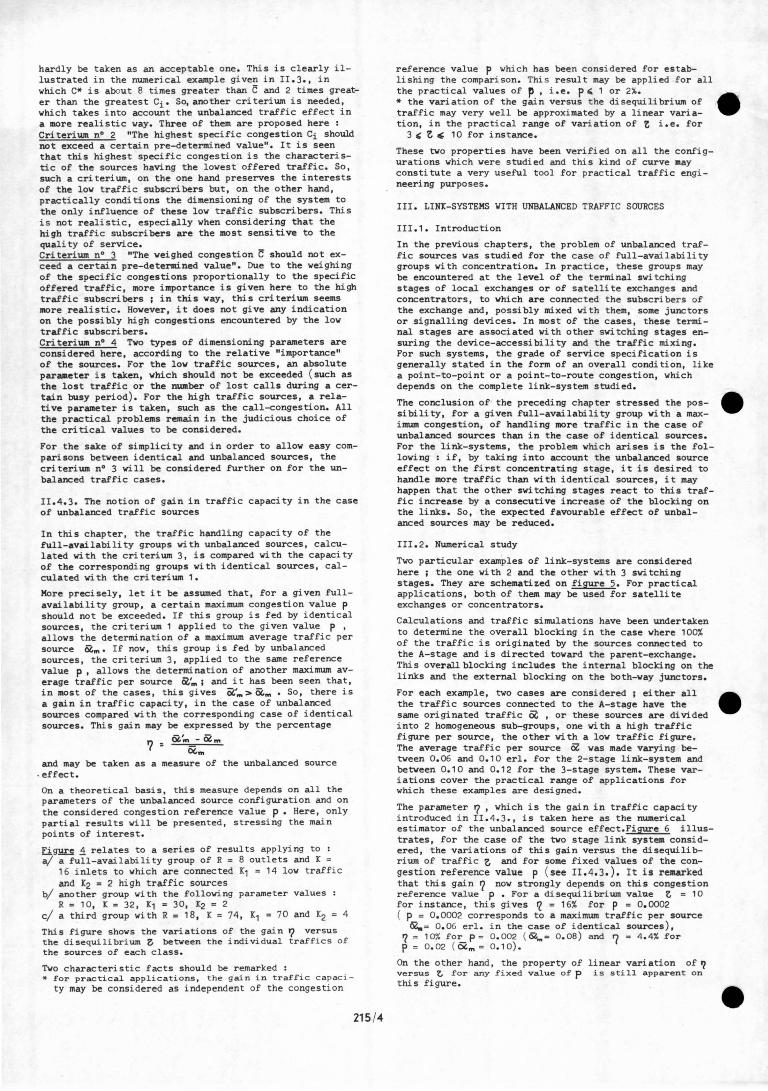
Ei~ ~ relates to a series of results applying to : ~ a full-availability group of R = 8 outlets and X =

16 inlets to which are connected K1 = 14 lo~ traffi c and K2 = 2 high traffic sources

bl another group with the following parameter values R = 10, X = 32, X1 = 30, X2 = 2

cl a third group with R = 18, K = 74, X1 = 70 and K2 4

This figure shows the variations of the gain? versus the disequilibrium ~ be~een the individual traffi cs of the sources of each class.

Two characteristic facts should be remarked : * for practical applications, the gain i n traffic c apac i ­

ty may be considered as independent of the congestion

215 /4

reference value p ~hich has been considered for estab­lishing the comparison. This result may be applied f or all the practical values of P , i .e. p" 1 or 2%. * the variation of the gain versus the disequilibrium of traffic may very well be approximated by a linear varia­tion, in the practical range of variation of 'l i.e. for

3 , ~ ~ 10 for instance.

These ~o properties have been verified on all the config­urations which were studied and this kind of curve may constitute a very useful tool for practical traffic engi ­neering purposes.

Ill. LINK-SYSTEMS WITH UNBALANCED TRAFFIC SOURCES

111.1. Introduction

In the previous chapters, the problem of unbalanced traf­fic sources was studied for the case of full-availability groups with concentration. In practice, these groups may be encountered at the level of the terminal switching stages of local exchanges or of satellite exchanges and concentrators, to ~hich are connected the subscri bers of the exchange and, possibly mixed with them, some junctors or signalling devices. In most of the cases, these termi­nal stages are associated with other switching stages en­suring the device-accessibility and the traffic mixing. For such systems, the grade of service specification is generally stated in the form of an overall condition, like a point-to-point or a point-to-route congestion, ~hich depends on the complete link-system studied.

The conclusion of the preceding chapter stressed the pos­sibility, for a given full-availability group ~ith a max­imum congestion, of handling more traffic in the case of unbalanced sources than in the case of identical sources. For the link-systems, the problem which arises is the fol­lo~ing : if, by taking into account the unbalanced source effect on the first concentrating stage, it is desired to handle more traffic than with identical sources, it may happen that the other switching stages react to ' this traf­fic increase by a consecutive increase of the blocking on the links. So, the expected favourable effect of unbal­anced sources may be reduced.

111.2. Numerical study

T~o particular examples of link-systems are considered here; the one wi th 2 and the other with 3 switching stages. They are schematized on figure 5. For practical applications, both of them may be used for satellite exchanges or concentrators.

Calculations and traffic simulations have been undertaken to determine the overall blocking in the case ~here 100% of the traffic is originated by the sources connected to the A-stage and is directed to~ard the parent-exchange. This overall blocking includes the internal blocking on the links and the external blocking on the both-~ay junctors.

For each example, ~o cases are considered; either all the tr'affic sources connected to the A-stage have the same originated traffic OG , or these sources are divided into 2 homogeneous sub-groups, one with a high traffic figure per source, the other with a low traffic figure. The average traffic per source OZ was made varying be­~een 0.06 and 0.10 erl. for the 2-stage link-system and be~een 0.10 and 0.12 for the 3-stage system. These var­iations cover the practical range of applications for which these examples are designed.

The parameter '? ' ~hich is the gain in traffic capaci ty introduced in 11.4.3., is taken here as the numerical estimator of the unbalanced source effect.Figure 6 illus­trates, for the case of the ~o stage link system consid­ered, the variations of this gain versus the disequilib­rium of traffic ~ and for some fixed values of the con­gestion reference value p ( see 11.4.3.). It is remarked that this gain? no~ strongly depends on this congestion reference value p • For a di sequi li bri um value ~ = 10 for instance, this gives ~ = 16% for p = 0.0002 ( p = 0.0002 corresponds to a maximum traffic per source ~= 0.06 erl. in the case of identical sources),

"l = 10% for:. P = 0.002 ( ~"'= 0.08) and 7 = 4.4% for p = 0.02 ( OG m = 0.10).

On the other hand, the property of linear variation of? versus Z, for any fixed value of P is still apparent on this figure.

•

•

•

•

•

•

•

•

, In the range of traffic considered for the 3-stage link system, the calculated and simulated results did not gi ve any significant difference between the congestion values obtained wi th identical sources or wi th unbalanced SOUrcES

So, for practical applications, the effect of unbalanced sources is null in this case.

All these results may be explained in the following gen­eral comments.

111.3 . General comments on the results and conclusion

Link-systems are designed for some acceptable grade of service values and this implies the practical traffic conditions in which they have to work. For satellite­exchanges and concentrators, this grade of service is mainly a mat·ter of an overall blocking toward the parent­exchange. For this overall blocking, and according to the traffic conditions considered, we have one out of the three following possi bilities.

a/ bl cl

the congestion enr ountered on the f i rst concentrat ing stage is predominant the external congestion on the trunks ( Erlang blocking) is predominant "-both congestions have more or less the same numerical importance on the overall congestion.

Since the possible unbalanced traffic effect affects the congestion on the first concentrating stage only, the fol­lowing general statement may easily be deduced: the larger the relative importance of the blocking on~e first concentrating stage on the overall blocking, the larger the possible unbalanced traffic effect.

This statement can be followed in the numerical results obtained in the examples. For the 3-stage system, the con­sidered traffic conditions correspond to the case bl and consequently, the unbalanced effect was found negligible. The 2-stage system is gradually passing from a state near­ly corresponding to the case a/ ( for OG", ~ 0.06), to a state nearly corresponding to the case bl ( for ~'" ~ 0.10) and the consequent decrease of the unbalanced traffic ef­fect has been noted .

In order to conclude comments on this chapter, a very at­tractive economical point must be stressed which consists in the possibility of reducing the number of trunks be­tween a satellite exchange or a concentrator and the par­ent exchange, this, by taking into account the unbalanced source effect. The following numerical example illustra~ this possibility, for the case of the 2-stage system con­sidered. With 32 identical sources per A-switch, at ~ = 0.08, 64 trunks are needed for handling the total

originated traffic A = 40. 92 erl. with an overall block­ing c* < 0. 002. Now, if on each A-swi tch 30 low traffic sources ( oc, = 0. 051) and 2 high traffic sources ( 062 = 0.51) are connected, only 60 trunks are needed for handling the same total traffic A = 40.92 erl. with a weighed overall-congestion C ~ 0.002. So, the economy is far from negligible in this case •

However, caution must be used in trying to realize such an economy because it is based on two important practical constraints :

a/ a perfect and precise knowledge of the traffic offered per source is required and bl a constant use is made here of the dimensioning criterium 3, which practical applica­tion in traffic engineering may. be discussed.

Bibliographical reference:

[1] J .P. DART0I5 and A.R. RODRI GUEZ "Traffic unbalances in small groups of subscribers" Vth I.T.C. New-York 1967 Electrical Communications Vol.43 N° 2, 1968.

215 /5

24 7=9ain in traffic capacity

22 I 16 inlets 8 outlets

32inltt' 10oull'" Flour. 4

20~~-===f=~t+----~--,L~--

18

16

14

12

74 inl.t. 18oull."

10t-~~~~T-~---Y------~~--4-----

~. d.sequilibrium ,/ of traffic

0'~~~~~-+4--~--6~~--4---9~~~--~11~

Example n~ 1 ~ Miscellaneou,

11

i! BWJ

Example n~ 2

Fioure 5

? = gain In traffic : eop~eity I I I 18 : (~in Preen,) : L'-I

; Flour. 6 I 16 __ ~ __ _: 1-_2_+-_ 14 ' : T : ; !

I i I j I

I ! i 12

10

4

3

2

'--i--- L-: I

I

I _1 __ . _1 __ _

I I 1

!

APPENDIX

I. THE MATHEMATICAL MODEL AND THE NOTATIONS

Here a mathematical model is presented which constitutes a generali zation of the one-stage full-availability group theory to more complex systems working under the lost call cleared assumptions.

N classes~i of sources are considered connected to the same network. Each class ~ . is an homogeneous class in the sense that i t is compos~d of Ki (finite or not) inde­pendent sources which are strictly identical for traffic view point. Each class i s characterized by its mathemat­ical laws for emissi on of the calls, for acceptation of these calls by the network and for release of these calls. Some notati ons have to be given in order to define these laws.

The system is said to be in the state ( j, •••• , jN) at the date t i f, at this date. there~e exactly j, calls in course originated by the class ~" •••• and jN calls from .gN. There, j = ~ '. is the total number of

i = , h calls i n course in the system at the considered date t.

Let be R. the maximum number of simultaneous calls origi­nated by1. t ... in course in the system. and R the maximum number of calls in course in the system. The so-called "L" limi tations will be used :

10 ~ j . .. R. '" R for all i

"L" 1. 1. ' 04.j .. R

The mathematical symbols and L represent the cor-( L) ( L)

responding equalities and sums with application of the "L" limi tations.

Law of emission of the calls

The conditional probability. knowing that the system is in the state (j ,. ..•• j . . •••• jN) at time t. that a call is attempted by anyon~ of the ~ree sources of the ~~ class. in the time interval ( t. t + dt) is Al..ji ' dt

with )\ij ' a time independent constant which is called "the :&. -~lass-rate-attempt". 1.

Law of acceptation of the calls

The conditional probability. knowing that the system is in the state ( j, •••• 'ji'n •••• jN) at time. t, and. a c~ll has been attempted by a ~.-class source 1.n the t1.me 1.n­terval ( t. t + dt). that tliis call is accepted is ;).i.,j4"j wi th \)i J'. J' a time independent constant such that

. ..... ' o ~ Vi J'. J' ~ " Vi R' J' = 0 for all i, and

t ... , '.L' v·· = 0 .I.,Ji,R

~.i.,j4Jj is called the acceptation coefficient ; it cor­responds to a selective reaction of the network to the call-attempts it receives. This reaction may depend on a lot of factors ; among them : the state of occupation of the network at the date of emission of the call-attempt. the strategy of acceptation appli ed for each type of call­attempt •••

Law of release of the calls

The conditional probability. knowing that the system is in the state ( j, •••• ,j .•••• 'jN) at time t, that a~. class-call be released1. in the time interval ( t,t+dt)1. is

t:"i,ji' dt wi th ~4.j .. a time independent constant which is called the ,g . -class release coeffi cient.

1

The stationary state

Under these conditions, the system follows a homogeneous, f i nite. permanent and discontinuous Markov's process. In its infinitesimal evolution. this process is characterized by its transi tion coefficients Ai,ii, , ~i.j.i. ,j and ~4j~ and these coefficients are assumed to be such

that a unique stationary state exists which corresponds to a true probability distribution. Therefore, this sta­tionary di stri bution is the unique soluti on of the follow­i ng l i near system :

215/6

(1.)

LN ~ ... ' J'. 1 J' 1 .A;J' l' P(j1'·" '1_1,jl~1,J.i.." ...• j .. ) + .i.:1 ' ... - , - ", .i.-

I:N U .. • PUp .... 'ji-1 ,J,i, +1 'j.i.+1 ..... .jN) l.:1 (. .L,J.i. +1

It is possible to obtain the explici t solution of this system if the following additional assumption is made: the acceptation coefficient ~i,j4 ,j may be wri t ten under the form \),i.,li.,j = e.i.,j,;:~ wi th e.i.,R.i. 0

for all i and \)R = 0

e.i.J ' may be interpreted as a coefficient of selection of the 1> calls. mainly depending on the type of the call­attempt and the number of calls of this type in cours e ~i is a congestion coefficient corresponding t o the state of occupation of the network.

In this case, this gives the following occupancy probabil-i ty distri bution . ,

p(jP .. .. .. . jN) ~ Plo ...... o).17~h.n ... It, i." J-1 N g"1 e A (L) hJ' i~} It: !;Li. "+1

with p(O, •••• O) given by

11. ADAPTATION TO THE TELEPHONE MODELS

In the telephone models, each coefficient of the above formulae may be simplified and expressed in £unction of the traffic terms. If Ai denotes the total offered traffic of the class ~i

Cif the call-congestion for the sources of~i and~.i. the reverse of the average 4 i -call-holding time. this gives the following relations :

a/

A . . -, K· - . . ) , ll... A;./Ki.. 4'Ji - \ .L JJ. ("'.I. 1-Ail1- Cil/K.i. for an Engset emission

process. bl ALIi;. Ai.l;'-.i. whatever be ji for a pure Erlang

emission process. cl AiJ·. a . forj1.'< K. and A.i.K' :O. fora .... 1. 1. I J,

truncated Erlang emission process.

( Note : For a group of K. trunks offering their calls to R devices, it is said to1. be a pure Erlang process when K. > R and a truncated Erlang process .... hen K. ~ R. The f6rmula Ai.,ii: A.i.-~i means that the Ki trunks ke enri tting their calls a: a constant rate Ai~i independently of the total number J. ofbusy trunks.ln the truncated case. the K. trunks are ~tting their calls at a constant rate cti '~4 only during the time that they are not fully occu­pied (i.e. for j . < K.). Only approximated relations be­tween a. and the1.reallf offered traffic A. can be written; one of them is a. # A . • For computation pkposes, a . is taken as the inp~t p~ameter for calculating the stite probabilities and A. is a-posteriori calculated with re­spect to these prob~bilities). On the other hand, the one-stage full availability are characterized by an acceptation coefficient such that

groups

~·L.ji,j ~R '

for 0 ~ ji ~ Ri and 0 ~ j < R and for all i

L , ~ 'J o and ~i,ji IR = 0 for all i

Finally the negative exponential distribution law of the holding times in each c~ass.gi ( average holding time= It:''i ) corresponds to e- .L)jA, = Ji '1:L.i.

Taking into account these simplifications. tHis gives the following general formula for the occupancy probability distri bution

.... i th p(O ••••• O) gi ven by

•

•

•

•

•

•

•

•

These formulae are of great interest because they cover the complete theory of the one-stage full-availability groups with or without identical sources •

Ill. SPECIFIC FORMULAE

111.1. Case of identical traffic sources

IlI.l.l. Engset case: lC > Rand lC finite

The input parameter for calculation is b defined by

b = A/K = 1- A(1-C)/K 1- oG(1-C)

where C is the call-congestion.

It gives Aj = . ( lC-j ).1:'. b for 0 ~ j ~ R and the previously

mentioned general formula leads to

A = b )'R(K-j).PU) j;O

c = (K-R). P(R)

l:R (K - j ) . P (j ) J:O

for 0 ~

B = Time-congestion = peR)

111.1.2. Erlang case lC ~ R

~ R

The input parameter for calculation is the total traffic A offered by the route. This gives the following formulae

P(j) toR A%t\ for O~ .;; R

C = B = P ( R)

111.2. Case of unbalanced traffic sources

The input parameters for calculations are:for each class of subscribers, bi defined by

b. - AliK4 .l - 1 - Ai (1-Cil/K4

and for each class of trunks, ai introduced in 11 and de­fined by

Q . _ A.i.,ji ~ - (lA.

(vi th ~ = Ai for a pure Erlang emission process and

ai # Ai for a truncated process)

111.2.1. Two different classes of subscribers

(IlI.2.1.1.)

vi th (L) 1,2

( IIl.2.1.2.)

(IIl.2.1.3.)

Similar formulae for A2 and C2

B (time-congestion) = , p( j1 j) .~ . , 2

J1+ Jz:R

215/7

111.2.2. One class of }Cl subscribers mixed with lC2 trunks

respective formulae

R LP {R- j2 .jz.l if ~2 > R

jz:R-R1

111.2.3. N distinct traffic sources

For each source Si' the input parameter considered is bi, as previously defined.

with

(L) {

ji = 0 or 1 for all i ,N. and 0 ~ L Jj, .;; R

id

111.3. Conclusions

This list of particular cases is not exhaustive. As already said, the general formulae given in 11 for the state prob-­ability distribution cover all possible source configura­tions, with or without unbalanced traffic, thus providing a very useful theoretical tool. A judicious choice of the input parameters for calculation allows a very easy compu­tation of these probabilities and of the resulting conges­tions and traffic offered, for each specific case.