Lossless Message Compression

Bachelor Thesis in Computer Science

Stefan Karlssonskn07007@student.mdh.se

Erik Hanssonehn05007@student.mdh.se

School of Innovation, Design and EngineeringMälardalens Högskola

Västerås, Sweden2013

ABSTRACTIn this thesis we investigated whether using compressionwhen sending inter-process communication (IPC) messagescan be beneficial or not. A literature study on lossless com-pression resulted in a compilation of algorithms and tech-niques. Using this compilation, the algorithms LZO, LZFX,LZW, LZMA, bzip2 and LZ4 were selected to be integratedinto LINX as an extra layer to support lossless messagecompression. The testing involved sending messages withreal telecom data between two nodes on a dedicated net-work, with different network configurations and messagesizes. To calculate the effective throughput for each algo-rithm, the round-trip time was measured. We concludedthat the fastest algorithms, i.e. LZ4, LZO and LZFX, weremost efficient in our tests.

KeywordsCompression, Message compression, Lossless compression,LINX, IPC, LZO, LZFX, LZW, LZMA, bzip2, LZ4, Effectivethroughput, Goodput

SAMMANFATTNINGI detta examensarbete har vi undersokt huruvida komprimer-ing av meddelanden for interprocesskommunikation (IPC)kan vara fordelaktigt. En litteraturstudie om forlustfri kom-primering resulterade i en sammanstallning av algoritmeroch tekniker. Fran den har sammanstallningen utsags al-goritmerna LZO, LZFX, LZW, LZMA, bzip2 och LZ4 forintegrering i LINX som ett extra lager for att stodja kom-primering av meddelanden. Algoritmerna testades genomatt skicka meddelanden innehallande riktig telekom-data mel-lan tva noder pa ett dedikerat natverk. Detta gjordes medolika natverksinstallningar samt storlekar pa meddelandena.Den effektiva natverksgenomstromningen raknades ut forvarje algoritm genom att mata omloppstiden. Resultatetvisade att de snabbaste algoritmerna, alltsa LZ4, LZO ochLZFX, var effektivast i vara tester.

Special thanks to:Ericsson Supervisor: Marcus JagemarEricsson Manager: Magnus SchlyterMDH Examiner: Mats BjorkmanIRIL Lab Manager: Daniel Flemstrom

1

Table of Contents

1 Introduction 3

1.1 Contribution . . . . . . . . . . . . . . . . . . . . . . . . . . . . . . . . . . . . . . . . . . . . . . . . . . . . . . . . 3

1.2 Structure . . . . . . . . . . . . . . . . . . . . . . . . . . . . . . . . . . . . . . . . . . . . . . . . . . . . . . . . . . 3

2 Method for literature study 3

3 Related work 4

4 Problem formulation 5

5 Compression overview 6

5.1 Classifications . . . . . . . . . . . . . . . . . . . . . . . . . . . . . . . . . . . . . . . . . . . . . . . . . . . . . . . 6

5.2 Compression factors . . . . . . . . . . . . . . . . . . . . . . . . . . . . . . . . . . . . . . . . . . . . . . . . . . . . 6

5.3 Lossless techniques . . . . . . . . . . . . . . . . . . . . . . . . . . . . . . . . . . . . . . . . . . . . . . . . . . . . 65.3.1 Null suppression . . . . . . . . . . . . . . . . . . . . . . . . . . . . . . . . . . . . . . . . . . . . . . . . . . 65.3.2 Run-length encoding . . . . . . . . . . . . . . . . . . . . . . . . . . . . . . . . . . . . . . . . . . . . . . . 65.3.3 Diatomic encoding . . . . . . . . . . . . . . . . . . . . . . . . . . . . . . . . . . . . . . . . . . . . . . . . . 75.3.4 Pattern substitution . . . . . . . . . . . . . . . . . . . . . . . . . . . . . . . . . . . . . . . . . . . . . . . . 75.3.5 Statistical encoding . . . . . . . . . . . . . . . . . . . . . . . . . . . . . . . . . . . . . . . . . . . . . . . . 75.3.6 Arithmetic encoding . . . . . . . . . . . . . . . . . . . . . . . . . . . . . . . . . . . . . . . . . . . . . . . . 75.3.7 Context mixing and prediction . . . . . . . . . . . . . . . . . . . . . . . . . . . . . . . . . . . . . . . . . . 75.3.8 Burrows-Wheeler transform . . . . . . . . . . . . . . . . . . . . . . . . . . . . . . . . . . . . . . . . . . . 85.3.9 Relative encoding . . . . . . . . . . . . . . . . . . . . . . . . . . . . . . . . . . . . . . . . . . . . . . . . . 8

5.4 Suitable algorithms . . . . . . . . . . . . . . . . . . . . . . . . . . . . . . . . . . . . . . . . . . . . . . . . . . . . 85.4.1 LZ77 . . . . . . . . . . . . . . . . . . . . . . . . . . . . . . . . . . . . . . . . . . . . . . . . . . . . . . . . 85.4.2 LZ78 . . . . . . . . . . . . . . . . . . . . . . . . . . . . . . . . . . . . . . . . . . . . . . . . . . . . . . . . 85.4.3 LZSS . . . . . . . . . . . . . . . . . . . . . . . . . . . . . . . . . . . . . . . . . . . . . . . . . . . . . . . . 85.4.4 LZW . . . . . . . . . . . . . . . . . . . . . . . . . . . . . . . . . . . . . . . . . . . . . . . . . . . . . . . . 95.4.5 LZMA . . . . . . . . . . . . . . . . . . . . . . . . . . . . . . . . . . . . . . . . . . . . . . . . . . . . . . . 95.4.6 LZO . . . . . . . . . . . . . . . . . . . . . . . . . . . . . . . . . . . . . . . . . . . . . . . . . . . . . . . . 95.4.7 LZFX . . . . . . . . . . . . . . . . . . . . . . . . . . . . . . . . . . . . . . . . . . . . . . . . . . . . . . . . 95.4.8 LZC . . . . . . . . . . . . . . . . . . . . . . . . . . . . . . . . . . . . . . . . . . . . . . . . . . . . . . . . . 95.4.9 LZ4 . . . . . . . . . . . . . . . . . . . . . . . . . . . . . . . . . . . . . . . . . . . . . . . . . . . . . . . . . 95.4.10 QuickLZ . . . . . . . . . . . . . . . . . . . . . . . . . . . . . . . . . . . . . . . . . . . . . . . . . . . . . . 95.4.11 Gipfeli . . . . . . . . . . . . . . . . . . . . . . . . . . . . . . . . . . . . . . . . . . . . . . . . . . . . . . . 95.4.12 bzip2 . . . . . . . . . . . . . . . . . . . . . . . . . . . . . . . . . . . . . . . . . . . . . . . . . . . . . . . . 95.4.13 PPM . . . . . . . . . . . . . . . . . . . . . . . . . . . . . . . . . . . . . . . . . . . . . . . . . . . . . . . . 95.4.14 PAQ . . . . . . . . . . . . . . . . . . . . . . . . . . . . . . . . . . . . . . . . . . . . . . . . . . . . . . . . 95.4.15 DEFLATE . . . . . . . . . . . . . . . . . . . . . . . . . . . . . . . . . . . . . . . . . . . . . . . . . . . . . 10

6 Literature study conclusions 10

6.1 Motivation . . . . . . . . . . . . . . . . . . . . . . . . . . . . . . . . . . . . . . . . . . . . . . . . . . . . . . . . . 10

6.2 Choice of algorithm and comparison . . . . . . . . . . . . . . . . . . . . . . . . . . . . . . . . . . . . . . . . . . . 10

7 Method 11

7.1 Test cases . . . . . . . . . . . . . . . . . . . . . . . . . . . . . . . . . . . . . . . . . . . . . . . . . . . . . . . . . 11

7.2 Data working set . . . . . . . . . . . . . . . . . . . . . . . . . . . . . . . . . . . . . . . . . . . . . . . . . . . . . 12

7.3 Formulas for effective throughput . . . . . . . . . . . . . . . . . . . . . . . . . . . . . . . . . . . . . . . . . . . . 12

8 Implementation 12

8.1 Test environment . . . . . . . . . . . . . . . . . . . . . . . . . . . . . . . . . . . . . . . . . . . . . . . . . . . . . 12

8.2 Compression algorithms . . . . . . . . . . . . . . . . . . . . . . . . . . . . . . . . . . . . . . . . . . . . . . . . . 138.2.1 LZO . . . . . . . . . . . . . . . . . . . . . . . . . . . . . . . . . . . . . . . . . . . . . . . . . . . . . . . . 138.2.2 LZFX . . . . . . . . . . . . . . . . . . . . . . . . . . . . . . . . . . . . . . . . . . . . . . . . . . . . . . . . 138.2.3 LZW . . . . . . . . . . . . . . . . . . . . . . . . . . . . . . . . . . . . . . . . . . . . . . . . . . . . . . . . 138.2.4 LZMA . . . . . . . . . . . . . . . . . . . . . . . . . . . . . . . . . . . . . . . . . . . . . . . . . . . . . . . 138.2.5 bzip2 . . . . . . . . . . . . . . . . . . . . . . . . . . . . . . . . . . . . . . . . . . . . . . . . . . . . . . . . 138.2.6 LZ4 . . . . . . . . . . . . . . . . . . . . . . . . . . . . . . . . . . . . . . . . . . . . . . . . . . . . . . . . . 14

9 Results 14

10 Conclusion 14

11 Discussion 16

12 MDH thesis conclusion 16

13 Future work 17

2

1. INTRODUCTIONThe purpose of compression is to decrease the size of thedata by representing it in a form that require less space.This will in turn decrease the time to transmit the dataover a network or increase the available disk space [1].

Data compression has been used for a long time. One earlyexample was in the ancient Greece where text was writtenwithout spaces and punctuation to save space, since paperwas expensive [2]. Another example is Morse code, whichwas invented in 1838. To reduce the time and space requiredto transmit text, the most used letters in English have theshortest representations in Morse code [3]. For example, theletters ‘e’ and ‘t’ are represented by a single dot and dash,respectively. Using abbreviations, such as CPU for CentralProcessing Unit, is also a form of data compression [2].

As mainframe computers were beginning to be used, newcoding techniques were developed, such as Shannon-Fanocoding [4,5] in 1949 and Huffman coding [6] in 1952. Later,more complex compression algorithms that did not only usecoding were developed, for example the dictionary basedLempel-Ziv algorithms in 1977 [7] and 1978 [8]. These havelater been used to create many other algorithms.

Compressing data requires resources, such as CPU time andmemory. The increasing usage of multi-core CPUs in today’scommunication systems increases the computation capac-ity quicker compared to the available communication band-width. One solution to increase the communication capacityis to compress the messages before transmitting them overthe network, which in theory should increase the effectivebandwidth depending on the type of data sent.

Ericsson’s purpose with this work was to increase the avail-able communication capacity in existing systems by simplemeans, without upgrading the network hardware or modi-fying the code of existing applications. This was done byanalysing existing compression algorithms, followed by in-tegrating a few suitable algorithms into the communicationlayer of a framework provided by Ericsson. The communica-tion layer in existing systems can then be replaced to supportcompression. Finally, testing was performed to determinethe most promising algorithms. Since this implementationwas used in Ericsson’s infrastructure, the message data wasvery specific. There was no need to test a variety of differentdata sets, i.e. the compression was done on data gatheredfrom a real system.

1.1 ContributionWe have tested how the performance of LINX IPC mes-sages of sizes between 500 and 1400 bytes sent over a simplenetwork are affected by implementing an extra layer of com-pression into LINX, and at which network bandwidths andmessage sizes it is beneficial to use such an implementation.We also provide a general idea of what types of compressionalgorithms to use when sending small sized messages over anetwork and what affects their performance.

1.2 StructureThis report starts with an introduction to compression, thepurpose of this work, the contribution and the structure ofthis report in Section 1. In Section 2 the method used to findsources for the literature study is described, followed by re-lated work in Section 3 where we summarize papers that arerelated to our work. Section 4 describes the task and what

we did and did not do in this thesis. Section 5 contains anoverview of how compression works, including compressionclassification, some of the techniques used in compressionand suitable compression algorithms for our work. In Sec-tion 6 we drew a conclusion from the literature study andmotivated which algorithms we chose to use in our work,as well as describing their properties. Section 7 describesthe method for the work. This section includes where weintegrated the chosen algorithms, how the message trans-fer was conducted, the test cases used, a description of thedata used in the tests and how we calculated the effectivethroughput. In Section 8 we describe how we integrated thecompression algorithms and where we found the source codefor them. Here we also describe the hardware used and thenetwork topology, i.e. the test environment. Section 9 con-tains the results of the tests and in Section 10 we draw aconclusion from the results. In Section 11 we discuss the re-sults, conclusion and other related topics that emerged fromour work. Section 12 contains the thesis conclusions thatare of interest for MDH. Finally Section 13 contains futurework.

2. METHOD FOR LITERATURE STUDYTo get an idea of the current state of research within the fieldof data compression, we performed a literature study. Infor-mation on how to conduct the literature study was found inThesis Projects on page 59 [9]. We searched in databasesusing appropriate keywords, such as compression, losslesscompression, data compression and text compression.

When searching the ACM Digital Library1 with the com-pression keyword, we found the documents PPMexe: Pro-gram Compression [10], Energy-aware lossless data compres-sion [11], Modeling for text compression [12], LZW-BasedCode Compression for VLIW Embedded Systems [13], Datacompression [1], Compression Tools Compared [14], A Tech-nique for High Ratio LZW Compression [15] and JPEG2000:The New Still Picture Compression Standard [16].

By searching the references in these documents for othersources, we also found the relevant documents A block-sortinglossless data compression algorithm [17], Data CompressionUsing Adaptive Coding and Partial String Matching [18], Amethod for construction of minimum redundancy codes [6],Implementing the PPM data compression scheme [19], Net-work conscious text compression system (NCTCSys) [20],A universal algorithm for data compression [7], Compres-sion of Individual Sequences via Variable-Rate Coding [8],Longest match string searching for Ziv-Lempel compression[21], A corpus for the evaluation of lossless compression al-gorithms [22], PPM Performance with BWT Complexity: ANew Method for Lossless Data Compression [23], The math-ematical theory of communication [4], PPM: one step topracticality [24], A Technique for High-Performance DataCompression [25], The Transmission of Information [5], DataCompression via Textual Substitution [26] and The DataCompression Book [27].

Searching the ACM Digital Library with the keywords loss-less compression yielded the additional documents Energyand Performance Evaluation of Lossless File Data Compres-sion on Server Systems [28] and An Analysis of the Burrows-Wheeler Transform [29].

1http://dl.acm.org/

3

We also searched the IEEE Xplore database2 using the key-words compression, lossless compression, data compression,high speed compression algorithm and text compression andfound the documents Lossless Compression Using EfficientEncoding of Bitmasks [30] and Improving Code Density Us-ing Compression Techniques [31], LIPT: a lossless text trans-form to improve compression [32], Unbounded Length Con-texts for PPM [33] and Scaling Down Off-the-Shelf DataCompression: Backwards-Compatible Fine-Grain Mixing [34].Searching the references in these we found the documentsAdaptive end-to-end compression for variable-bandwidth com-munication [35], Adaptive online data compression [36], Fine-Grain Adaptive Compression in Dynamically Variable Net-works [37], Efficient end to end data exchange using config-urable compression [38], Gipfeli - High Speed CompressionAlgorithm [39] and The hitchhiker’s guide to choosing thecompression algorithm for your smart meter data [40].

To find more information about specific algorithms we foundin the other documents, we searched Google Scholar3 usingthe keywords LZMA, LZSS, LZW, LZX, PPM, DEFLATE,BZIP2, LZ4, LZO, PAQ. This way, we found the papersHardware Implementation of LZMA Data Compression Al-gorithm [41], The relative efficiency of data compression byLZW and LZSS [42] and Lossless Compression Based on theSequence Memoizer [43]. Looking at the references in thesepapers we also found the paper A Comparative Study OfText Compression Algorithms [44].

We also searched the IEEE Global History Network4 usingthe keyword compression to find the page History of LosslessData Compression Algorithms [45].

While searching Google with the key words effective through-put compression and data transmission compression to findmore information on how to calculate effective throughputwe stumbled upon a few papers addressing the effect of com-pression in network applications and protocols. The pa-pers found were Improving I/O Forwarding Throughput withData Compression [46], Robust Data Compression of Net-work Packets [47] and A Comparison of Compressed andUncompressed Transmission Modes [48].

Finally, to find some more recent benchmarks, we also searchedGoogle using the keywords compression benchmarks to findthe page Compression Benchmarks [49] and LZ4 - ExtremelyFast Compression algorithm [50].

3. RELATED WORKIn 1949, C. Shannon and R. Fano invented Shannon-Fanocoding [4,5]. Using this algorithm on a given block of data,codes are assigned to symbols in a way that is inverselyproportional to the frequency at which the symbols appear.Two years later, D. Huffman developed a very similar butmore efficient coding algorithm called Huffman coding [6].This technique is often used in combination with other mod-ern algorithms, for example with the Burrows-Wheeler trans-form in bzip2 [51] and with LZ77 or LZSS in the DEFLATEalgorithm [52].

In 1977, A. Lempel and J. Ziv developed a new compressionalgorithm called LZ77 which uses a dictionary to compress

2http://ieeexplore.ieee.org/3http://scholar.google.com/4http://www.ieeeghn.org/

data [7]. The dictionary is dynamic and generated usinga sliding window over the input data. A year later, theydeveloped the LZ78 algorithm, which generates and uses astatic dictionary [8]. Many algorithms have been developedbased on the LZ77 and LZ78 algorithms, such as DEFLATE[52], the Lempel-Ziv-Markov chain algorithm (LZMA) [53]and the Lempel-Ziv-Welch algorithm (LZW) [25].

One category of algorithms used in data compression thatis not based on the LZ77 and LZ78 algorithms is Predictionby Partial Matching (PPM). PPM algorithms have been de-veloped since the mid-1980s by for example Cleary and Wit-ten [18], but have become more popular as the amount ofRAM in computers has increased. The PPM algorithms usesthe previous symbols in the data stream to predict which thenext symbol is. One version called PPMd, developed by D.Shkarin in 2002 [24], aimed to have complexity comparableto the LZ77 and LZ78 algorithms. He showed that the al-gorithm could offer compression ratio comparable to LZ77and bzip2 but with lower memory requirements and fasterrate of compression, or offer better compression ratio thanLZ77 and bzip2 but with higher memory requirements andcompression time, depending on the settings used.

The Burrows-Wheeler transform (BWT), invented by M.Burrows and D. Wheeler in 1994, does not compress dataitself but it makes the data more suited for compression withother algorithms [17]. Used with simple and fast algorithms,such as a move-to-front coder, they were able to show thatthe algorithm had compression ratio comparable with sta-tistical modellers, but at a rate of compression comparableto Lempel-Ziv algorithms.

In Adaptive end-to-end compression for variable-bandwidthcommunication [35] by Knutsson and Bjorkman from 1999,messages were compressed using an adaptive algorithm whichchanged the compression level depending on the length ofthe network queue. They showed that the effective band-width could be increased on networks with 1-3 Mbit/s through-put by compressing the data using a computer with a 133 MHzCPU.

In Robust Data Compression of Network Packets [47], S.Dorward and S. Quinlan experimented with different com-pression algorithms to improve the performance of packetnetworks. The experiments were conducted on 125 and 1600byte packet sizes on a network with 10 kbit/s, 100 kbit/s,1 Mbit/s and 10 Mbit/s link speed. They concluded thatspeed is important when compressing network packets, es-pecially if the bandwidth is large when compared to theavailable computational capacity.

In 2001 N. Motgi and A. Mukherjee proposed a Networkconscious text compression system (NCTCSys) [20] whichcompressed text based data and could be integrated on ap-plication level into different text based network transfer pro-tocols like HTTP, FTP and SMTP. The compression appli-cations tested were bzip2 and gzip together with LIPT (Alossless text transform to improve compression [32]). Withthis method they where able to reduce the data transmissiontime by 60-85%.

On the Distributed Computing Systems conference in 2005,C. Pu and L. Singaravelu presented Fine-Grain AdaptiveCompression in Dynamically Variable Networks [37] wherethey applied adaptive compression on data packets using

4

a fine-grain mixing strategy which compressed and sent asmuch data as possible and used any remaining bandwidthto send uncompressed data packets. The compression algo-rithms they tried were gzip, bzip2 and LZO which all havedifferent properties regarding rate of compression and com-pression ratio. Their experiments were conducted on a net-work with up to 1 Gbit/s bandwidth and concluded thatimprovement gained when using the different compressionalgorithms was reduced as the physical bandwidth increasedto the point where it was worse than non-compressed trans-mission. The maximum bandwidth where compression wasbeneficial was different for each of the algorithms.

In Energy-aware lossless data compression [11] a comparisonof several lossless compression algorithms was made by K.Barr and K. Asanovic, where not only compression ratio andrate of compression was measured but also memory usage.This study concludes that there are more factors to considerthan only the compression ratio, i.e. a fast algorithm withhigh compression ratio probably uses a lot more memorythan its counterparts. This is something that needs to beconsidered for implementation on the target architecture.

Y. Wiseman wrote The relative efficiency of data compres-sion by LZW and LZSS [42] in 2007 where he compared thecompression algorithms LZW and LZSS which are based onLZ77 and LZ78, respectively. The study shows that de-pending on how many bits are used for the pointer, and thenumber of bits for the length component in LZSS, the re-sults will vary. With too many bits, each pointer will takeup too much space, and with too few bits the part of the filewhich can be pointed to will be too small. The efficiency ondifferent file formats is also compared, and it is concludedthat LZSS generally yields a better compression ratio, butfor some specific types of files, where the number of point-ers generated by LZW and LZSS are almost equal, LZWperforms better since its pointers are smaller than those ofLZSS.

In the paper Improving I/O Forwarding Throughput withData Compression [46] B. Welton, D. Kimpe, J. Cope et al.investigated if the effective bandwidth could be increased byusing data compression. They created a set of compressionservices within the I/O Forwarding Scalability Layer andtested a variety of data sets on high-performance computingclusters. LZO, bzip2 and zlib were used when conductingtheir experiments. For certain scientific data they observedsignificant bandwidth improvements, which shows that thebenefit of compressing the data prior to transfer is highlydependent on the data being transferred. Their results sug-gest avoiding computationally expensive algorithms due tothe time consumption.

In 2011 A Comparative Study Of Text Compression Algo-rithms by S. Shanmugasundaram and R. Lourdusamy waspublished in the International Journal of Wisdom BasedComputing [44]. They presented an overview of differentstatistical compression algorithms as well as benchmarkscomparing the algorithms. The benchmarks were focusedon algorithms based on LZ77 and LZ78 but also includedsome other statistical compression techniques. The proper-ties that were compared in the benchmarks were compres-sion ratio and rate of compression.

In The hitchhiker’s guide to choosing the compression al-gorithm for your smart meter data [40], M. Ringwelski, C.Renner, A. Reinhardt et al. performed tests on compres-sion algorithms to be implemented in Smart Meters5. Theytested compression ratio, rate of compression and memoryconsumption for different algorithms. Besides the test re-sults, which are relevant to us, they also suggest that theprocessing time of the algorithms are of high importance ifthe system runs on battery.

In November 2012 M. Ghosh posted the results of a com-pression benchmark [49] done with a self-made parallel com-pression program called Pcompress [54] which contains Cimplementations of LZFX, LZMA, LzmaMt6, LZ4, libbsc,zlib and bzip2. He also showed that some of the algorithmsused can still be optimized, for example he optimized LZMAby using SSE instructions which improved the rate of com-pression. The results are fairly new, which makes them veryrelevant to our work when deciding which algorithms to in-tegrate.

R. Lenhardt and J. Alakuijala wrote Gipfeli - High SpeedCompression Algorithm for the 2012 Data Compression Con-ference where they created their own compression algorithmbased on LZ77 called Gipfeli [39]. Gipfeli is a high-speedcompression algorithm designed to increase the I/O through-put by reducing the amount of data transferred. Gipfeliis written in C++ and the compression ratio is said to besimilar to that of zlib but with three times faster rate ofcompression.

4. PROBLEM FORMULATIONThe task was to take advantage of compression by integrat-ing it into the supplied communication framework used bythe Ericsson Connectivity Packet Platform (CPP). The im-plementation should be done in user-mode, to make it easierto maintain the code if the kernel is upgraded. This wouldhowever come at the cost of restricted access to resourcesthat are used in kernel-space. We did a literature studyto investigate existing compression algorithms. Based onthe study, a few promising algorithms were selected for in-tegration and testing to analyse the effect of compressionin the existing environment. The communication was donewith LINX Inter-Process Communication (IPC) [55] withthe compression as an extra layer which hopefully wouldincrease the communication capacity, i.e. each LINX IPCmessage was compressed and decompressed.

The tests were performed with varying message sizes on dif-ferent network bandwidths, as well as network topologies, tosee if the performance of the algorithms changed. The testswere done without any other traffic present, which meantthat the tests had full utilization of the bandwidth.

We did not test the effect of compression when communi-cating between processes internally in the CPU. Neither didwe develop our own compression algorithm due to time con-straints and we did not use adaptive compression methods.The benchmark did not include an analysis of memory usagefor the algorithms, instead we left this for future work.

5System that sends wireless sensor signals to a target device6Optimized and multi-threaded LZMA implementation

5

5. COMPRESSION OVERVIEWThis section contains a general introduction to compressionand its terms.

5.1 ClassificationsThe two most distinct classifications of compression algo-rithms are lossy and lossless. Lossy compression reducesthe data size by discarding information that requires largeamounts of storage but is not necessary for presentation.For example by removing sound frequencies not normallyperceived by human hearing in an audio file, as in the MP3audio format. Lossy compression has proven to be effec-tive when applied to media formats such as video and au-dio [27]. However, when using lossy compression it is im-possible to restore the original file due to removal of essen-tial data. Because of this, lossy compression is not optimalfor text-based data containing important information [45].Lossless data compression can be achieved by various tech-niques that reduces the size without permanently remov-ing any data. Compared to lossy compression, the originaldata can be restored without losing any information. Loss-less data compression can be found everywhere in comput-ing. Some examples are to save disk space, transmittingdata over a network, communication over a secure shell etc.Lossless compression is widely used in embedded systemsto improve the communication bandwidth and memory re-quirements [30].

Some examples of compression used in different media for-mats can be seen in Table 1.

Compression type Image Audio VideoNoncompressed RAW WAV CinemaDNGLossy JPEG MP3 MPEGLossless PNG FLAC H.264

Table 1: Compression used in typical media formats

5.2 Compression factorsCompressing data requires execution time and memory todecrease the size of the data. The compression factors usedto describe this are rate of compression, compression ratioand memory usage.

The rate of compression, also known as compression speed, isthe time it takes to compress and decompress data. The timeit will take for an algorithm to compress and decompress thedata is highly dependent on how the algorithm works.

Compression ratio is how much a set of data can be com-pressed with a specific algorithm, i.e. how many times smallerin size the compressed data is compared to the noncom-pressed data. The definition of compression ratio is:

R =Size before compression

Size after compression(1)

This definition is sometimes referred to as compression fac-tor in some of the papers used in the literature study. Wechose to use this definition instead due to the cognitive per-ception of the human mind [56], where larger is better.

Memory usage is how much memory a specific algorithm useswhile compressing and decompressing. Like rate of com-pression, the memory usage is highly dependant on how the

algorithm works. For example if it needs additional datastructures to decompress the data.

5.3 Lossless techniquesSince we were required to use lossless compression, this sec-tion summarizes some of the existing techniques used whenperforming lossless data compression. Different variants ofthe techniques discussed in this section has spawned over theyears. Because of this, techniques with similar names canbe found, but in the end they work in the same way. Forexample scientific notation works as Run-length encoding,where 1 000 000 is represented as 1e6 or 1× 106 in scientificnotation and as 1Sc06 in Run-length encoding (here Sc isthe special character, corresponding to ∅ in our examplesbelow).

5.3.1 Null suppressionNull or blank suppression is one of the earliest compressiontechniques used and is described in [1,57]. The way the tech-nique works is by suppressing null, i.e. blank, characters toreduce the number of symbols needed to represent the data.Instead of storing or transmitting all of the blanks ( ) in adata stream, the blanks are represented by a special symbolfollowed by a number representing the number of repeatedblanks. This would reduce the number of symbols neededto represent the data. Since it needs two symbols to encodethe repeated blanks, at least three blanks needs to be re-peated to use this technique, else no compression would beachieved. An example can be seen in Table 2 where the first

With invisible blanks With visible blanks

Date Name Date Name27-11-1931 Ziv 27-11-1931 Ziv

Table 2: Null suppression example

column is what a person would see and the second columnis the actual data needed to form this representation. If wewould transfer the information as it is we also need to trans-fer all the blanks. The first two blanks before “Date” cannotbe compressed but the other blanks can. If we were to trans-fer the information line by line and use null suppression wewould instead send the following data stream:

1. Date∅C11Name

2. 27-11-1931∅C10Ziv

Where the symbol ∅ is the special compression indicatorcharacter, Ci is an 8-bit integer encoded as a character andi is the decimal value of the integer in our example. Thismeans that the maximum number of repeating blanks thatcan be encoded this way is 256, since this is the maximumvalue of an 8-bit integer.

By encoding the example in Table 2 and using Equation (1)the compression ratio is

R =43

27≈ 1.59

The total size was reduced by 37.2%.

5.3.2 Run-length encodingLike null suppression, Run-length encoding tries to suppressrepeated characters as described in [1,25,44,45,48,57]. The

6

difference is that Run-length encoding can be used on alltypes of characters, not only blanks. Run-length encodingalso works similar to null suppression when indicating thata compression of characters has been performed. It uses aspecial character that indicates that compression follows (inour case we use ∅), next is the character itself and last thenumber of repeats. To achieve any compression, the numberof repeated characters needs to be at least four. In the exam-

Original string Compressed stringCAAAAAAAAAAT C∅A10T

Table 3: Run-length Encoding example

ple in Table 3 we reduced the number of characters from 12to 5, saving 58% space with a compression ratio of 2.4 whenusing Equation (1) on the preceding page. If Run-length en-coding would be used on a repetition of blanks it would yieldan extra character (the character indicating which charac-ter was repeated) when compared to Null suppression. Theuse of a mixture of several techniques is suggested due tothis [57].

5.3.3 Diatomic encodingDiatomic encoding is a technique to represent a pair of char-acters as one special character, thus saving 50% space or acompression ratio of 2. This technique is described in [57].The limitation is that each pair needs a unique special char-acter. The number of special characters that can be usedare however limited, since each character consists of a fixednumber of bits. To get the most out of this technique onefirst needs to analyse the data that is going to be compressedand gather the most common pairs of characters, then usethe available special characters and assign them to each ofthe most common pairs.

5.3.4 Pattern substitutionThis technique is more or less a sophisticated extension ofDiatomic encoding [57]. Patterns that are known to repeatthemselves throughout a data stream are used to create apattern table that contains a list of arguments and a set offunction values. The patterns that are put into the tablecould for example be reserved words in a programming lan-guage (if, for, void, int, printf etc.) or the most commonwords in an English text (and, the, that, are etc.). Instead ofstoring or transmitting the full string, a character indicatingthat a pattern substitution has occurred followed by a valueis stored or transmitted in place of the string. When de-coding, the pattern substitute character and the subsequentvalue is looked up in the table and replaced with the string itrepresents. The string could contain the keyword itself plusthe preceding and succeeding spaces (if any exists), whichwould yield a higher compression ratio due to the increasedlength of the string.

5.3.5 Statistical encodingStatistical encoding is a technique used to determine theprobability of encountering a symbol or a string in a specificdata stream and use this probability when encoding the datato minimize the average code length L, which is defined as:

L =

n∑i=1

LiPi (2)

Where n is the number of symbols, Li is the code lengthfor symbol i and Pi is the probability for symbol i. In-cluded in this category are widely known compression meth-ods such as Huffman coding, Shannon-Fano encoding andLempel-Ziv string encoding. These techniques are describedin [6–8,44,45,48,57].Huffman coding is a technique which reduces the averagecode length of symbols in an alphabet such as a human lan-guage alphabet or the data-coded alphabet ASCII. Huffmancoding has a prefix property which uniquely encodes sym-bols to prevent false interpretations when deciphering theencoded symbols, such that an encoded symbol cannot bea combination of other encoded symbols. The binary treethat is used to store the encoded symbols is built bottomup, compared to the Shannon-Fano tree which is built topdown [6, 44, 48, 57]. When the probability of each symbolappearing in the data stream has been determined, they aresorted in order of probability. The two symbols with the low-est probability are then grouped together to form a branchin the binary tree. The branch node is then assigned thecombined probability value of the pair. This is iterated withthe two nodes with the lowest probability until all nodes areconnected and form the final binary tree. After the tree hasbeen completed each edge is either assigned the value one orzero depending on if it is the right or left edge. It does notmatter if the left edge is assigned one or zero as long as itis consistent for all nodes. The code for each symbol is thenassigned by tracing the route, starting from the root of thetree to the leaf node representing the symbol.Shannon-Fano encoding works in the same way as Huff-man coding except that the tree is built top down. When theprobability of each symbol has been determined and sorted,the symbols are split in two subsets which each form a childnode to the root. The combined probability of the two sub-sets should be as equal as possible. This is iterated untileach subset only contains one symbol. The code is createdin the same way as with Huffman codes. Due to the way theShannon-Fano tree is built it does not always produce theoptimal result when considering the average code length asdefined in Equation (2).Lempel-Ziv string encoding creates a dictionary of en-countered strings in a data stream. At first the dictionaryonly contains each symbol in the ASCII alphabet where thecode is the actual ASCII-code [57]. Whenever a new stringappears in the data stream, the string is added to the dictio-nary and given a code. When the same word is encounteredagain the word is replaced with the code in the outgoingdata stream. If a compound word is encountered the longestmatching dictionary entry is used and over time the dictio-nary builds up strings and their respective codes. In someof the Lempel-Ziv algorithms both the compressor and de-compressor needs to construct a dictionary using the exactsame rules to ensure that the two dictionaries match [44,57].

5.3.6 Arithmetic encodingWhen using Arithmetic encoding on a string, characterswith high probability of occurring are stored using fewerbits while characters with lower probability of occurring arestored using more bits, which in the end results in fewer bitsin total to represent the string [1, 44,45,58].

5.3.7 Context mixing and predictionPrediction works by trying to predict the probability ofthe next symbol in the noncompressed data stream by firstbuilding up a history of already seen symbols. Each symbolthen receives a value between one and zero that represents

7

the probability of the symbol occurring in the context. Thisway we can represent symbols in the specific context thathas high occurrence using fewer bits and those with low oc-currence using more bits [59].Context mixing works by using several predictive modelsthat individually predicts whether the next bit in the datastream will be zero or one. The result from each model arethen combined by weighted averaging [60].

5.3.8 Burrows-Wheeler transformBurrows-Wheeler Transform, BWT for short, does not ac-tually compress the data but instead transforms the data tomake it more suited for compression and was invented by M.Burrows and D. Wheeler in 1994 [17, 45]. This is done byperforming a reversible transformation on the input stringto yield an output string where several characters (or setof characters) are repeated. The transformation is done bysorting all the rotations of the input string in lexicographicorder. The output string will then be the last character ineach of the sorted rotations. BWT is effective when usedtogether with techniques that encodes repeated charactersin a form which requires less space.

5.3.9 Relative encodingRelative encoding, also known as delta filtering, is a tech-nique used to reduce the number of symbols needed to rep-resent a sequence of numbers [41,57]. For example, Relativeencoding can be useful when transmitting temperature read-ings from a sensor since the difference between subsequentvalues is probably small. Each measurement, except the firstone, is encoded as the relative difference between it and thepreceding measurement as long as the absolute value is lessthan some predetermined value. An example can be seen inTable 4.

16.0 16.1 16.4 16.2 15.9 16.0 16.2 16.116.0 .1 .3 -.2 -.3 .1 .2 -.1

Table 4: Relative Encoding example

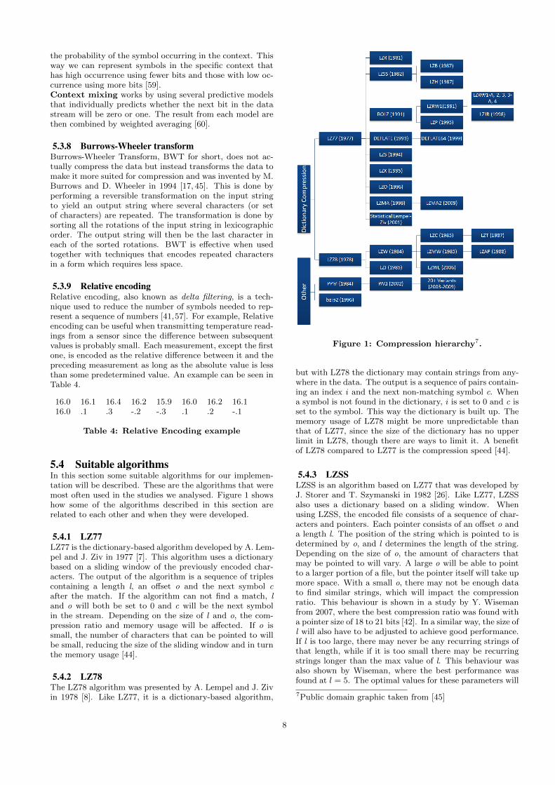
5.4 Suitable algorithmsIn this section some suitable algorithms for our implemen-tation will be described. These are the algorithms that weremost often used in the studies we analysed. Figure 1 showshow some of the algorithms described in this section arerelated to each other and when they were developed.

5.4.1 LZ77LZ77 is the dictionary-based algorithm developed by A. Lem-pel and J. Ziv in 1977 [7]. This algorithm uses a dictionarybased on a sliding window of the previously encoded char-acters. The output of the algorithm is a sequence of triplescontaining a length l, an offset o and the next symbol cafter the match. If the algorithm can not find a match, land o will both be set to 0 and c will be the next symbolin the stream. Depending on the size of l and o, the com-pression ratio and memory usage will be affected. If o issmall, the number of characters that can be pointed to willbe small, reducing the size of the sliding window and in turnthe memory usage [44].

5.4.2 LZ78The LZ78 algorithm was presented by A. Lempel and J. Zivin 1978 [8]. Like LZ77, it is a dictionary-based algorithm,

Figure 1: Compression hierarchy7.

but with LZ78 the dictionary may contain strings from any-where in the data. The output is a sequence of pairs contain-ing an index i and the next non-matching symbol c. Whena symbol is not found in the dictionary, i is set to 0 and c isset to the symbol. This way the dictionary is built up. Thememory usage of LZ78 might be more unpredictable thanthat of LZ77, since the size of the dictionary has no upperlimit in LZ78, though there are ways to limit it. A benefitof LZ78 compared to LZ77 is the compression speed [44].

5.4.3 LZSSLZSS is an algorithm based on LZ77 that was developed byJ. Storer and T. Szymanski in 1982 [26]. Like LZ77, LZSSalso uses a dictionary based on a sliding window. Whenusing LZSS, the encoded file consists of a sequence of char-acters and pointers. Each pointer consists of an offset o anda length l. The position of the string which is pointed to isdetermined by o, and l determines the length of the string.Depending on the size of o, the amount of characters thatmay be pointed to will vary. A large o will be able to pointto a larger portion of a file, but the pointer itself will take upmore space. With a small o, there may not be enough datato find similar strings, which will impact the compressionratio. This behaviour is shown in a study by Y. Wisemanfrom 2007, where the best compression ratio was found witha pointer size of 18 to 21 bits [42]. In a similar way, the size ofl will also have to be adjusted to achieve good performance.If l is too large, there may never be any recurring strings ofthat length, while if it is too small there may be recurringstrings longer than the max value of l. This behaviour wasalso shown by Wiseman, where the best performance wasfound at l = 5. The optimal values for these parameters will

7Public domain graphic taken from [45]

8

be dependent on the data being compressed. In the studyby Wiseman the data was plain text from King James Bible.

5.4.4 LZWLZW was developed by T. Welch in 1984, and was designedto compress without any knowledge of the data that wasbeing compressed [25]. It is based on the LZ78 algorithmand is used for example in the GIF format. The dictionaryused is initialized with the possible elements, while phrasesof several elements are built up during compression [13]. Ithas somewhat fallen out of use because of patent issues, al-though the patents have now expired [27]. LZW applies thesame principle of not explicitly transmitting the next non-matching symbol to LZ78 as LZSS does to LZ77 [44]. Justas in LZSS, the offset pointer size chosen affects the memoryusage of the algorithm [42]. The compression ratio for LZWis often not as good as with many other algorithms, as seenin the study by S. Shanmugasundaram and R. Lourdusamy,where the compression ratio for most types of data is worsecompared to LZ78, LZFG, LZ77, LZSS, LZH and LZB [44].For some data, for example files containing a lot of nulls,LZW may outperform LZSS as shown by Y. Wiseman [42].

5.4.5 LZMAThe Lempel-Ziv-Markov chain algorithm was first used inthe 7z format in the 7-Zip program. It is based on LZ77 anduses a delta filter, a sliding dictionary algorithm and a rangeencoder. The delta filter is used to make the data bettersuited for compression with the sliding window dictionary.The output from the delta filter is in form of differencesfrom previous data. The sliding dictionary algorithm is thenapplied to the output of the delta filter. Finally, the outputfrom the sliding dictionary is used in a range encoder whichencodes the symbols with numbers based on the frequencyat which the symbols occur [41]. LZMA uses a lot of memoryand requires a lot of CPU resources, but seems to yield abetter compression ratio than most algorithms except somePPM variants [40,49].

5.4.6 LZOLZO is an algorithm developed by M. Oberhumer whichis designed for fast compression and decompression [61]. Ituses LZ77 with a small hash table to perform searches. Com-pression requires 64 KiB of memory while decompressionrequires no extra memory at all. The results from a studycomparing the memory usage, speed and ratio of compress,PPMd, LZO, zlib and bzip2 by K. Barr and K. Asanovic [11]confirms this. LZO is the fastest of the tested algorithms,with the least amount of memory used. The compressionratio was worse than the other algorithms, but still compa-rable with for example compress. This algorithm is also im-plemented in Intel Integrated Performance Primitives sinceversion 7.0 [62], which means it might be even faster thanin the benchmarks by Barr and Asanovic if implementedcorrectly.

5.4.7 LZFXLZFX [63] is a small compression library based on LZF byM. Lehmann. Like LZO, it is designed for high-speed com-pression. It has a simple API, where an input and outputbuffer and their lengths are specified. The hash table sizecan be defined at compile time. There are no other com-pression settings to adjust.

5.4.8 LZCLZC was developed from LZW and is used in the Unix utilitycompress. It uses codewords beginning at 9 bits, and doublesthe size of the dictionary when all 9-bit codes have been usedby increasing the code size to 10 bits. This is repeated untilall 16-bit codes have been used at which point the dictionarybecomes static [11]. If a decrease in compression ratio isdetected, the dictionary is discarded [27]. In the study byK. Barr and K. Asanovic [11], they found that compresswas relatively balanced compared to the other algorithms,not being the best or worst in any of the categories. Thedata used for compression in this study was 1 MB of theCalgary corpus and 1 MB of common web data.

5.4.9 LZ4LZ4 is a very fast compression algorithms based on LZ77.Compressing data with LZ4 is very fast but decompressingthe data is even faster and can reach speeds up to 1 GB/s, es-pecially for binary data [64]. LZ4 is used in some well knownapplications like GRUB, Apache Hadoop and FreeBSD.

5.4.10 QuickLZQuickLZ is one of the fastest compression library in theworld, compressing and decompressing data in speeds ex-ceeding 300 Mbit per second and core. It was developedby L. Reinhold in 2006 [65]. It features an auto-detectionof incompressible data, a streaming mode which results inoptimal compression ratio for small sets of data (200-300byte) and can be used with both files and buffers. QuickLZis easy to implement, is open source and has a commercialand GPL license.

5.4.11 GipfeliA high-speed compression algorithm based on LZ77 whichwas created by R. Lenhardt and J. Alakuijala [39].

5.4.12 bzip2bzip2 compresses files using move-to-front transform, Burrows-Wheeler transform, run-length encoding and Huffman cod-ing [51]. In the study by K. Barr and K. Asanovic, it wasthe one of the slowest and most memory requiring algorithmsbut offered high compression ratio.

5.4.13 PPMThe development of PPM algorithms began in the mid-1980s. They have relatively high memory usage and com-pression time, depending on the settings used, to achievesome of the highest compression ratios. PPM algorithmshave been said to be the state of the art in lossless data com-pression [60]. One suitable PPM algorithm is the PPMd, orPPMII, algorithm by D. Shkarin, which seems to have goodperformance for both text and non-text files [24]. PPMd isone of the algorithms used in WinRAR [11]. K. Barr and K.Asanovic compared this algorithm to LZO, bzip2, compressand zlib and showed that it had the best compression ratioof these algorithms [11]. The memory usage can be varied,but in these tests PPMd used more memory than the otheralgorithms. The only other algorithm that had lower rate ofcompression was bzip2.

5.4.14 PAQPAQ is an open source algorithm that uses a context mix-ing model to achieve compression ratios even better thanPPM [60]. Context mixing means using several predictivemodels that individually predicts whether the next bit in the

9

data stream will be 0 or 1. These results are then combinedby weighted averaging. Since many models are used in PAQ,improvements to these models should also mean a slight im-provement for PAQ [43]. The high compression ratio comesat the cost of speed and memory usage [60].

5.4.15 DEFLATEThe DEFLATE algorithm was developed by P. Katz in 1993[45]. As described in RFC1951 [52], the DEFLATE algo-rithm works by splitting the input data into blocks, whichare then compressed using LZ77 combined with Huffmancoding. The LZ77 algorithm may refer to strings in pre-vious blocks, up to 32 kB before, while the Huffman treesare separate for each block. This algorithm is used in forexample WinZip and gzip. Benchmarks on this algorithm,in form of the zlib library, were made by K. Barr and K.Asanovic which showed that it had worse compression ratiothan for example bzip2, but was faster and used less mem-ory. However, it was not as fast and memory efficient asLZO.

6. LITERATURE STUDY CONCLUSIONSThis section will summarize the results of the literaturestudy and include the algorithms chosen for integration andthe motivation to why they were chosen.

6.1 MotivationWhen comparing compression algorithms the most impor-tant factors are rate of compression, compression ratio andmemory usage as describes in Section 5.2 on page 6. Mostof the time there is a trade-off between these factors. Afast algorithm that uses minimal amounts of memory mighthave poor compression ratio, while an algorithm with highcompression ratio could be very slow and use a lot of mem-ory. This can be seen in the paper by K. Barr and K.Asanovic [11].

Our literature study concluded that compressing the databefore transferring it over a network can be profitable underthe right circumstances.

If the available bandwidth is low and the processing powerof the system can compress the data in a short amount oftime or significantly reduce the size of the data, the actualthroughput can be increased. For example if one could com-press the data without consuming any time at all and at thesame time reduce the size of the data by a factor of two, theactual bandwidth would be increased by 100% since we aretransferring twice the amount of data in the same amountof time.

An algorithm that has high compression ratio is desirablebut these algorithms take more time than those with lowercompression ratio, which means that it will take longer timebefore the data can begin its journey on the network. On theother hand, if the transfer rate of the network is high, com-pressing the data can negatively affect the effective through-put. Thus a fast algorithm with low compression ratio canbe a bottleneck in some situations. By increasing the amountof allocated memory an algorithm has access to an increasein compression ratio can be achieved, however the amountof memory is limited and can be precious in some systems.The size and the content of the noncompressed data can alsobe a factor when it comes to compression ratio.

In our type of application, i.e. compressing the data, trans-

ferring it from one node to another followed by decompress-ing it, fast algorithms are usually the best. However thereare some circumstances that can increase the transmissiontime and therefore change this. Adaptive compression is atechnique used to adaptively change the compression algo-rithm used when these kind of circumstances changes, whichin turn can increase the effective throughput.

To investigate the effect of all these factors, we tried to selectone algorithm that performs well for each factor. A list ofthe most common algorithms was made, and we then lookedat the properties of each of these algorithms. A key note toadd is that we also made sure that we could find the sourcecode for all the algorithms chosen.

6.2 Choice of algorithm and comparisonBased on the literature study we selected the algorithms seenin Table 5. Since the time frame of this thesis was limited, wealso took into account the ease of integrating each algorithm.We also tried to pick algorithms from different branches asin seen the compression hierarchy Figure 1 on page 8. Oneof our theories was that since we were sending LINX IPCmessages, the speed of the algorithm would be importantbecause the messages would probably be quite short andcontain specific data. This was also one of the conclusionswe made from the literature study, but since we did ourtests on different network bandwidths with specific messagedata and size we needed a verification of the conclusion.Due to this we selected some slow algorithms even thoughit contradicted the conclusion.

LZMA was chosen because of the benchmark results in [49]and [40], it also achieves better compression than a few otheralgorithms [45]. Ghosh made his own more optimized ver-sion of LZMA and showed that the algorithm still can beimproved by parallelization [49], which should be optimalfor the future if the trend of increasing the amount of coresin CPU:s continues. The LZMA2 version also takes advan-tage of parallelization, however we could not find a multi-threaded version designed for Linux and it would be tootime consuming to implement it ourselves. Our supervisorat Ericsson also suggested that we looked at LZMA. An-other reason why we chose LZMA is because it has highcompression ratio but is rather slow which goes against theconclusion we made with the literature study, thus we canthen use LZMA to verify our conclusion.

LZW was chosen because it has decent factors overall. Itis also based on LZ78 while LZMA and LZO are based onLZ77. The patent on LZW expired in 2003. Because of thisvery few of the papers in the literature study has used LZW(some of them have used LZC which derives from LZW)therefore it could be interesting to see how it will perform.

bzip2 was chosen because of the benchmarks in [11, 49]. Ituses Move-To-Front transform, BWT, Huffman coding and

LZO bzip2 LZW LZFX LZMA LZ4S Fast Medium Medium Fast Slow FastR Low High Medium Low High LowM Low High Medium ? High Low

Table 5: Comparison of compression speed (S), com-pression ratio (R) and memory usage (M ) for algo-rithms.

10

RLE [51], and is completely separated from the LZ algo-rithms as seen in Figure 1 on page 8. Like LZMA, it is alsoa rather slow algorithm with high compression ratio, how-ever it should be a lot faster than LZMA but still slowerthan LZFX [49].

LZFX [63] was chosen because it is very fast, which can beseen in the benchmarks made by [49]. The compression ratiois however very low. The source code is also very small andsimple to use which made it optimal as a first test integra-tion.

LZO was chosen for the same reasons as LZFX: it is fastbut has low compression ratio and is easy to integrate. LZOand LZFX should have been optimal for our application ac-cording to the conclusion we made from the literature study,which was that fast algorithms are preferred.

LZ4 was chosen because it is very fast which can be seenin the benchmark by Collet [50]. It is also open source andeasy to integrate.

Some suitable algorithms were discarded or replaced, likeQuickLZ, PPMd, zlib and Gipfeli. The reason why we didnot integrate QuickLZ was because we discovered it very latein the project. The source code for PPMd was too complexand time consuming to analyse due to the lack of commentsand documentation, instead we chose bzip2. Gipfeli is writ-ten in C++ and therefore not supported “out of the box”in our implementation. zlib was discarded because it hasproperties comparable to some of the algorithms we chose;if we had chosen zlib we would have too many algorithmswith the same properties.

7. METHODTo determine the effect of compression when applied to LINXIPC messages that are transferred over a network, we firstneeded a suitable environment where the tests would be per-formed. We started by installing and configuring two serverswhere the tests would be performed. The idea was to con-struct a dedicated network where no other network trafficwas present to maximize the available bandwidth and tomake sure that each test was performed under the sameconditions regardless of when it was conducted. To test theeffect of different network bandwidths we configured the linkspeed of the servers interface connected to the data networkto 10, 100 and 1000 Mbit/s and performed the tests for eachbandwidth.

To get a general idea of how and where the actual compres-sion and decompression was performed we needed to famil-iarize ourselves with the provided communication frameworkby analysing the source code. We were provided with anearly prototype that already had LZFX integrated, whichgave us a general idea on how to integrate the other al-gorithms. The source code for the selected algorithms wasanalysed and edited to fit the provided communication frame-work. The compression and decompression was integrateddirectly into the LINX library as an extra layer to extendthe functions that are handling the Inter-Process Communi-cation, as seen in Figure 2. The test application then usedthe LINX library to send IPC messages between the senderand receiver. The sender, called pong, compresses a mes-sage (if compression is selected) and sends the message tothe receiver, called ping, which decompresses the messagefollowed by immediately compressing the message again and

sending it back to pong. Before sending the message, pongadds the current time to the message header. When thetransfer was complete the application used this timestampto calculate the Round-trip Time (RTT) of the message. Weadded a global variable in the LINX library that containedthe compression ratio, which was used by pingpong to calcu-late the average compression ratio for consecutive messagescompressed with the same algorithm as well as printing itout to the user. The message flow can be seen in Figure 2.

Figure 2: Message flow with compression as an extralayer in LINX

7.1 Test casesThe real telecom message data was exported from a Wire-shark8 log. While analysing the Wireshark log, we noticedthat the messages were sent with a throughput of 14 Mbit/s.This could be because the bandwidth was low or the networkload was high. However, we had 10, 100 and 1000 Mbit/sdedicated throughput when our tests were performed, i.e.no other traffic was present. Together with this informa-tion and the factors in Section 6 on the preceding page, weconstructed the test cases that can be seen below.

For 10, 100, and 1000 Mbit/s network bandwidth

– Send 5000, 10000 and 20000 messages, respectively,with telecom signal data of size 500, 700, 1000 and1400 byte

– Compress and decompress the messages with LZO,LZFX, LZMA, bzip2, LZW, LZ4 and without com-pression

– Acquire the average round-trip time and compressionratio

– Calculate the effective throughput using the averageround-trip time

Note that there was only one concurrent message on thenetwork at any given time, i.e. we do not send a streamof messages. This means that one message was sent andthe next message was not sent until the previous messagereturned.

8http://www.wireshark.org/

11

As a last test we determined the maximum throughput forour application by sending many large messages over a longperiod of time while at the same time monitoring the through-put using iftop. This was done to see if we could utilizeone hundred percent of the maximum available bandwidth.

To verify that the available bandwidth was correct we usediperf in TCP mode. We used TCP mode since we use LINXwith TCP connections.

7.2 Data working setThe data set used in the experiments was taken from a dumpof traffic data that was acquired by sniffing the traffic ofa node in a real telecom network. From this dump, 100packets were exported as static arrays to a C header fileusing Wireshark. The exported packets were not filtered forany specific senders or receivers. To fill the payload of themessages in our experiment, we looped through the arrays inthe header file and copied the data. Initial test runs showedthat the protocol header of each packet could be compressedto a higher degree than the payload of the packet. Becauseof this, we excluded the headers of the packets to give theworst-case scenario. The total amount of data, excludingprotocol headers, was approximately 20kB.

7.3 Formulas for effective throughputIn our experiment, the throughput B is defined as

B =Dc

t(3)

where Dc is the size of the compressed data and t is the timerequired to send that data between the two nodes. Thismeans the time to compress and uncompress the data isalso included in t. While running the tests for a specificbandwidth, B should be constant and Dc and t should varydepending on the compression algorithm used.

The effective throughput Be, also called goodput, is definedas

Be =D

t(4)

where D is the size of the data before compression and t isthe same as in Equation (3). In our tests D will be constant.If we use no compression, the compressed size of the dataDc will be equal to the size of the noncompressed data D,which means that by using Equation (3) and Equation (4),we get B = Be in the case of sending noncompressed data.To calculate the change in effective throughput from usingsome compression algorithm A, we calculate the quotient QA

between BeA and B, where BeA is the effective throughputfor algorithm A

QA =BeA

B=

D/tAD/tUC

=⇒ Q =tUC

tA(5)

Here, tA is the time when using algorithm A and tUC isthe time when sending noncompressed data. The effectivethroughput for algorithm A will then be

BeA = QAB =tUC

tAB (6)

8. IMPLEMENTATIONIn this section we describe how we setup the test environ-ment and implemented the compression algorithms chosen.

8.1 Test environmentThe test environment is shown in Figure 3 where the “Con-trol Network” is the network to access the servers where thetests were done. The connection between server 1 and 2,called “Data Network” in Figure 3, is where the communi-cation was done. The “Data Network” is where we config-ured the bandwidth by setting the link speed on the servers,while the link speed of the switch remained the same inall tests. We also tested how the performance is affectedwhen removing the switch between the servers and connect-ing them point-to-point. Both networks have 1000 Mbit/snetwork capacity. The servers have all the software neededto perform the tests. This includes a test program thatsends noncompressed and compressed LINX IPC messagesusing the selected compression algorithms as seen in Fig-ure 2 on the previous page. The servers runs Ubuntu Linux12.10 (Quantal Quetzal) with kernel version 3.5.0-28-genericx86 64. The specification of the server hardware can be seenin Table 6.

Figure 3: Hardware setup used in the tests

CPU 2 x AMD Opteron® 6128 2.00 GHz- Physical cores per CPU: 8- Max threads per CPU: 8- L1 instr. cache per CPU: 8 × 64 kB- L1 data cache per CPU: 8 × 64 kB- L2 Cache per CPU: 8 × 512 kB- L3 Cache per CPU: 2 × 6 MB

Memory Samsung DDR3 32 GB- Clock Speed: 1333 MHz

HDD Seagate 250 GB- RPM: 7200- I/O transfer rate: 300 MB/s- Cache: 8 MB

NIC Intel 82576 Gigabit Network Connection- Data rate: 10/100/1000 Mbps- Number of ports: 2

Table 6: Server 1 and 2 hardware specification

12

8.2 Compression algorithmsThe algorithms were integrated directly into the LINX li-brary, more specifically into ../liblinx/linx.c. The methodlinx_send_w_s has been extended to compresses the mes-sages with the selected algorithm while the linx_receive

method handles the decompression. In these methods theRTT and compression ratio were also calculated. The testapplication, pingpong, that uses the LINX library to sendand receive messages was used to select which compressionalgorithm to use, how many messages that should be sent,the content and size of each message and where to sendthe messages. Here we also calculated the average RTTand the average compression ratio. pingpong also fills themessage payload with data. In our case we call the func-tion fill_buffer where the first parameter fill_method

determines which method to use. One of the methods is touse real telecom data by calling the function init_buffer-

_from_pkts, which is implemented in pkt1_to_100.h. Thisfunction fills the payload buffer with real telecom data asdescribed in Section 7.2 on the preceding page.

8.2.1 LZOThe source code used for LZO was taken from the offi-cial website [61]. We used the lightweight miniLZO versionsince all that was needed was the compress and decompressfunctions. The files minilzo.c, minilzo.h, lzodefs.h andlzoconf.h were included directly into ../liblinx/linx.c.Compression was then done by using the lzo1x_1_compress

function, while decompression was done by using the lzo1x_-decompress function. Both functions take pointers to the in-put and output buffers, as well as the size of the input bufferby value and the size of the output buffer as a pointer. Thenumber of bytes written to the output buffer will be writtento the address of the output buffer pointer when the func-tion returns. The compression function also takes a pointerto a memory area that is used as working memory. The sizeof the working memory used was the default size.

8.2.2 LZFXFor LZFX, we used the source code found on [63]. The fileslzfx.c and lzfx.h were included in ../liblinx/linx.c

without any modifications. Compression and decompres-sion was then performed by calling the lzfx_compress andlzfx_decompress methods, respectively. Pointers to the in-put and output buffers are passed to both the decompressand compress functions. The size of the input buffer is sentby value, while the size of the output buffer is sent as apointer. When the functions return, the number of byteswritten to the output buffer is stored in the address of thispointer.

8.2.3 LZWThe source code used for LZW is based on M. Nelson’s ex-ample source code which was modified in 2007 by B. Banicato use buffers instead of files [66]. To be able to use the codein our application we made the following changes:

– Modified the source to work without the main-methodso that we could use the encode and decode method di-rectly, this was done by moving the memory allocationinto encode and decode.

– Changed the interface for encode and decode to take apointer to the output buffer and the size of the bufferinstead of allocating the buffer in the functions.

– Made the function calls re-entrant by replacing mostof the static variables with function parameters.

– Added checks to avoid reading or writing outside thebuffers and some small optimizations.

– Change the way fatal errors was handled by returninga value instead of terminating the application. Zeromeans the execution was successful, negative one in-dicates that the output buffer was too small or thecompressed size was larger than the original size andnegative two are fatal errors which terminates our testapplication.

LZW does not take any other arguments, however it is pos-sible to redefine the number of bits used for the code-wordsby changing the value of the BITS constant. We did sometest runs and came to the conclusion that 9 bits was optimalfor our data.

8.2.4 LZMAThe source code used for LZMA was the one included inthe LZMA SDK version 9.20 by 7-zip [53]. The files neededto compress and decompress using LZMA were: LzFind.c,LzFind.h, LzHash.h, LzmaDec.c, LzmaDec.h, LzmaEnc.c, Lz-maEnc.h and Types.h. To compress and decompress mes-sages the methods LzmaEncode and LzmaDecode were used.LzmaEncode required additional properties to determine howthe compression would be done, e.g. dictionary size, com-pression level, whether to use an end-mark or not etc. Whencalling LzmaDecode the properties used when encoding mustbe known. We chose to insert the properties in the begin-ning of each message. We performed some test runs withreal telecom data to determine appropriate values for eachproperty. The values we selected can be seen in Table 7.

Property Valuelevel 3dictSize 65536lc 3lp 0pb 2algo 0fb 32btMode 2numHashBytes 2mc 32writeEndMark 1numThreads 1

Table 7: LZMA encode and decode properties

8.2.5 bzip2To integrate bzip2 we used version 1.0.6 of the library lib-

bzip2 [51], which we compiled and installed on the sys-tem. Encode and decode methods were implemented intolinx.c and the libbzip2 library is linked in when buildingthe LINX library as well as the test application pingpong.The block size for compression was set to the smallest pos-sible value, 100 kB, since the size of the messages that werecompressed is at most a few kilobytes. The workFactor pa-rameter is used to determine when to use a slower, but moredeterministic, fallback algorithm. We tested different values

13

for this parameter on the real telecom data, but saw no dif-ference. This should mean the data we used is not near theworst-case, because the fallback algorithm is only used forworst-case data. We therefore used the default value. In thedecompress function, the small parameter is used to switchto a slower algorithm that uses at most 2300 kB of memory.Since the literature study showed that fast algorithms wereto prefer, we used the faster version of the function withhigher memory requirements.

8.2.6 LZ4We used the official source code for LZ4 made by Y. Col-let [50]. We decided to use the normal version of LZ4 andnot the multi-threaded version since we did not use multi-threading support for the other algorithms. Some of themdid not even have support for multi-threading, thus mak-ing it more fair. The files needed to integrate LZ4 werelz4.c, lz4.h, lz4_decode.h and lz4_encode.h. We didnot need to change the source code at all, we simply callthe LZ4_compress and LZ4_decompress_safe methods forcompressing and decompressing. Pointers to the input andoutput buffers were passed to these functions, as well asan integer specifying the size of the input data. The de-compression function also takes an argument that specifiesthe maximum size of the output buffer, while it is assumedin the compression function that the output buffer is of atleast the same size as the input buffer. Both functions re-turns the number of bytes written to the output buffer, incase of success. In order to avoid stack overflow, we neededdynamic memory allocation and therefore changed the valueof HEAPMODE to 1.

9. RESULTSThe results from the tests when using a switch on the datanetwork can be seen in Figure 4, 5 and 6, while the mea-surements from the point-to-point connection can be seen inFigure 7, 8 and 9. All the measurements were calculated ac-cording to Equation (6) on page 12. The lines representsthe average effective throughput for one concurrent mes-sage when using the different compression algorithms andno compression. The available link speed can be seen atthe top of each figure, which is also the theoretical max-imum throughput. As a final test we measured the max-imum throughput for the test application as described inSection 7.1 on page 11. The result of this test can be seenin Table 8.

Connection type Maximum ThroughputSwitched 261 Mbit/s

Point-to-point 265 Mbit/s

Table 8: Maximum throughput for the test applica-tion with point-to-point and switched connection.

Figure 10 shows the average compression ratio for all thealgorithms used when compressing LINX IPC messages ofsize 500, 700, 1000 and 1400 byte.

10. CONCLUSIONWhen compressing LINX IPC messages, some factors hadimpact on whether it was beneficial or not, in terms of ef-fective throughput. If the time spent on transferring themessages was high, compared to the time spent compress-ing and decompressing the messages, an increase in efficient

network throughput could be achieved. Regardless of if thetime spent transferring the messages depends on low net-work bandwidth or a high number of hops, the compressionand decompression time will be such a small part of the totaltransfer time that it will be profitable to use compression.This means that the choice of algorithm depends on the sizeof the messages, as well as the properties of the network,such as the complexity and available bandwidth. In ourcase the fastest algorithms, that still achieved a relativelyhigh compression ratio, were best suited. This was also theconclusion we made from the literature study.

LZ4 and LZO performs almost equally and are the mosteffective of all the algorithms we tested. They are both de-signed to be very fast, just as LZFX. However, LZFX isalways a few steps behind both LZ4 and LZO, and this gapseems to increase with higher link speed. This could be theeffect of lower compression ratio, as seen in Figure 10 onpage 16, or possibly slightly longer compression and decom-pression time. LZ4 was slightly better than LZO, most ofthe time achieving a few percent higher effective throughput,and in worst case performing equal to LZO.

The performance of LZW is low because the compressionratio does not increase much when the size of the messageincreases, compared to other algorithms. This is probablybecause we chose to use a low number of bits for the code-words, due to the small size of the messages.

LZMA achieved the highest compression ratio of all thetested algorithms, but since the compression and decom-pression time was high, we did not see any improvement ofthe effective throughput. However, what we can see wasthat LZMA gained more than the other algorithms fromincreased complexity in the network, which means that itmight be the most beneficial algorithm in more complex net-works.

bzip2 was the worst of the algorithms tested since it hadtoo low compression ratio compared to the other algorithms.The compression and decompression time was also the longestof all algorithms.

Looking back at Table 5 on page 10 the predictions werecorrect for LZO, LZFX, LZMA and LZ4. bzip2 seemed tohave a longer execution time than LZMA and the compres-sion ratio was very low, while we expected it to be high. Theachieved compression ratio for LZW was also lower than wehad expected.

As discussed in Section 6 on page 10, the compression mightbecome a bottleneck when transferring messages. When thelink speed was set to 1000 Mbit/s, regardless of whether weused point-to-point or switched connection, we got negativeeffects when using any of the compression algorithms. Intable 8 we can see that the maximum throughput for thetest application was around 260 Mbit/s, which means thatwe never used the maximum available throughput when thelink speed was set to 1000 Mbit/s. However, the through-put was approximately 14 Mbit/s when analysing the logsfor real telecom traffic. This means it should be beneficialto use compression in the real environment since we sawimprovement on bandwidths up to 100 Mbit/s.

14

Figure 4: Average effective throughput per messageusing various algorithms with 10 Mbit/s link speedand a switched network.

Figure 5: Average effective throughput per messageusing various algorithms with 100 Mbit/s link speedand a switched network.

Figure 6: Average effective throughput per mes-sage using various algorithms with 1000 Mbit/s linkspeed and a switched network.

Figure 7: Average effective throughput per messageusing various algorithms with 10 Mbit/s link speed.

Figure 8: Average effective throughput per messageusing various algorithms with 100 Mbit/s link speed.

Figure 9: Average effective throughput per mes-sage using various algorithms with 1000 Mbit/s linkspeed.

15

Figure 10: Compression ratio for all the algorithmsusing Equation (1) on page 6.

11. DISCUSSIONWe can see in figure 4 to 9 that the effective throughput isconsistently higher when using switched connections, com-pared to point-to-point connections. This means that thecomplexity of the network, i.e. more hops, has an impacton the effective throughput when using compression. Thetime to compress the message is constant, i.e. the numberof hops has no impact on the compression time. Howeverthe time to transfer the message will increase, especially ifthe switches in the network use store-and-forward. Store-and-forward means that the switch must receive the wholeframe before it begins to forward it to the recipient. A keynote to add is that we were only using one switch, while ina real environment there might be several switches betweenthe sender and receiver, thus increasing the transfer timeeven more.

When sending messages with 1400 byte payload size, thetransfer time decreased for noncompressed messages whencompared to messages of size 1000 byte. This was only no-ticeable when the link speed was set to 1000 Mbit/s. Wethink the decrease in time depends on the fact that the TCPmessage is split in two segments, since the default MaximumTransmission Unit (MTU) size is 1500 byte.

In Figure 10, we can see that the compression ratio for bzip2was very low even when compared to the fastest algorithms,which should have the lowest compression ratio. This couldbe due to the fact that the data being compressed is notsuitable for this algorithm, but according to Burrows andWheeler [17], the Burrows-Wheeler transform should workwell for both text and binary data. It might instead dependon the fact that each message that is being compressed isrelatively small. bzip2 uses blocks of size 100 kB to 900 kBwhen compressing, which means it would probably be moreefficient for larger amounts of data.

LZMA has the highest compression ratio among all the al-gorithms we tested. If the execution time could be de-creased by parallelization while at the same time retainingthe high compression ratio, the effective throughput could beincreased and thus reduce the gap between LZMA and thefast algorithms. When sending messages with LINX IPC,the compression and decompression is only performed at theend-nodes, i.e. the compression and decompression time isindependent of the network topology. Another advantage ofalgorithms with high compression ratio is when consideringvery complex networks. With higher compression ratio, theamount of data that needs to be forwarded at each hop will

be smaller, which also means that the amount of time spentforwarding packages decreases. If the transmission time islong, compared to the compression and decompression time,it should be beneficial to use algorithms with high compres-sion ratio. LZMA, as is, should be a good candidate whenconsidering implementation of adaptive message compres-sion in the future.

The maximum throughput for the test application was de-termined to be 261 Mbit/s with switched connection and265 Mbit/s with point-to-point connection. The maximumthroughput can be increased for the test application by re-moving unnecessary instructions and optimizing the code.A key note to add is that this was a prototype application,which means that the final implementation will not necessar-ily need to calculate the compression ratio, RTT and otherdiagnostic information. This also means that the perfor-mance for compressed messages will increase more than fornoncompressed messages in the final implementation.

Since we decided not to use any kind of parallelization, thetime to compress and decompress data with any of the al-gorithms chosen can be decreased by taking advantage ofopportunities in the source code which can benefit from par-allel execution. This however comes with the cost of unpre-dictable cache behaviour and increased complexity of thecode. The hardware we used to perform the tests, as seen inTable 6 on page 12, might not be optimal in our case whenparallel execution is absent, since the architectural design ofthe CPU:s is based on using multiple cores simultaneouslywhen executing. If parallelization was introduced when com-pressing and decompressing data, the total execution timeshould be decreased for compressed messages while the exe-cution time for noncompressed messages should be the same.This in turn would increase the effective throughput whenusing Equation (6) on page 12.

We had hoped to be able to limit the available bandwidthto other speeds than 10, 100 or 1000 Mbit/s by using aswitch with Quality of Service (QoS) support in the datanetwork. We had set up the test environment in such a way,but when we started testing we noticed that the rate limitof the switch did not affect the results when sending smallamounts of data. We suspect that this was because the ratelimit in the switch is only an average over a period of time.The link speeds of the interfaces on the switch must stillbe set to 10, 100 or 1000 Mbit/s, which means that this isthe rate at which a single packet will be sent on the link.To get the correct rate, a stream of packets must be sent.However when transferring a stream of messages, the RTT ofeach messages was not comparable to when sending a singlemessage. This meant we had to limit our measurements to10, 100 and 1000 Mbit/s bandwidth.

A prediction for the future is that slow algorithms, withhigh compression ratio, will gain more from the increase inCPU power over time, compared to fast algorithms with lowcompression ratio. Both network speeds and the number oftransistors in a CPU increase at a very high rate, but up-grading CPU:s to a newer generation is probably easier andless expensive than upgrading the entire network infrastruc-ture to be able to handle higher speeds.

12. MDH THESIS CONCLUSIONThe thesis project has worked excellent overall and we feltlike we have learnt a lot, while at the same time gaining ex-

16

perience in how it is to work in our field of education. Prob-lems always arise, but it was nothing we could not handle.For example, it was not easy to find open source algorithmswhich were efficient, written in C and had buffer to buffersupport. It was also really hard to determine if the sourcecode for an algorithm was efficient and would even work.This problem was solved by trial and error. We decided touse git as version handler, however it did not work as well aswe thought. The initial repositories failed to maintain thestructure of the framework that was provided by Ericsson.In the end we packed the framework versions in tar-ballsand used git to maintain a repository of different versions ofthe framework. Limiting the physical bandwidth was not aseasy as we had expected. In the end we decided to give upthe idea of limiting the bandwidth, other than setting linkspeeds on the servers interface.

We had no problems setting up the test environment, includ-ing using NAT to get internet access for the servers, accountadministration on Linux etc. Implementing the algorithmswas neither a problem, one of the reasons being the greatsupport from Marcus, as well as the framework being welldocumented and easy to understand. Communication withour supervisors and examiner worked great and we felt veryprovided for. Ongoing feedback throughout the project re-sulted in higher motivation and a feeling that the work wasof importance. Finding papers, books and other sourcesabout compression and transferring data on networks waseasy. This resulted in the wast amount of references whichwas used to gain knowledge about the subject. Getting allthe pre-requirements from Ericsson, e.g. framework and realtelecom data, needed to conduct the project worked withoutproblems.

The work environment was great and we felt that the taskwas at an appropriate level of difficulty, while still being funand interesting. The knowledge gained from earlier coursesat MDH has been very useful in the project. For exam-ple Parallella system, Datakommunikation, Operativsystem,Datorarkitektur, Kompilatorteori, Datakommunikation i nat-verk, Linux grundkurs, Avancerad C/C++ etc.

In the end we feel very satisfied with our work and hope theresults will come in handy in the future.

13. FUTURE WORKThese are some topics that we did not have time to inves-tigate in our thesis, but which may be of interest in thefuture:

– Implement more algorithms, maybe even our own ver-sion.

– Implement LINX IPC compression on the target hard-ware.

– Adaptive compression with several different algorithms.

– Investigate the energy usage of the algorithms due tothe popularity of Green Power.

– Modify some promising algorithm based on the datathat is being compressed.

– Hardware implementation of some algorithm.

– Implement parallel versions of all the algorithms tested.

– Test more fast algorithms (zlib, QuickLZ, Gipfeli etc.).

– Optimize the test application by removing calculationsand unnecessary operations.

– Analyse the memory usage for different algorithms.

REFERENCES[1] Debra A. Lelewer and Daniel S. Hirschberg. Data

compression. ACM Computing Surveys, 19(3):261–296,September 1987.

[2] Ross N. Williams. Adaptive Data Compression.Springer, 1st edition, 1991.

[3] Stephen Wolfram. Some Historical Notes. In A NewKind of Science, chapter Processes, page 1069.Wolfram Media, 2002.

[4] C E Shannon. The mathematical theory ofcommunication. 1963. MD computing computers inmedical practice, 14(4):306–17, 1948.

[5] Robert Mario Fano. The Transmission of Information.Massachusetts Institute of Technology, ResearchLaboratory of Electronics, 1949.

[6] D.A. Huffman. A method for the construction ofminimum-redundancy codes. Proceedings of theInstitute of Radio Engineers, pages 1098 –1101,September 1952.

[7] Jacob Ziv and Abraham Lempel. A universalalgorithm for sequential data compression. IEEETransactions on Information Theory, 1977.

[8] Jacob Ziv and Abraham Lempel. Compression ofIndividual Sequences via Variable-Rate Coding. IEEETransactions on Information Theory, 5, 1978.

[9] M. Berndtsson, J. Hansson, B. Olsson, and B. Lundell.Thesis Projects. Springer, 2nd edition, 2008.

[10] Milenko Drinic, Darko Kirovski, and Hoi Vo. PPMexe:Program Compression. ACM Transactions onProgramming Languages and Systems, 29(1):1–31,2007.

[11] Kenneth C. Barr and Krste Asanovic. Energy-awarelossless data compression. ACM Transactions onComputer Systems, 24(3):250–291, August 2006.

[12] I A N H Witten and John G Cleary. Modeling for textcompression. ACM Computing Surveys, 21(4):557–591,1989.

[13] Chang Hong Lin and Wayne Wolf. LZW-Based CodeCompression for VLIW Embedded Systems. InProceedings of the conference on Design, automationand test in Europe, page 30076, 2004.

[14] Kinglsey G. Morse Jr. Compression Tools Compared.Linux Journal, 2005(137):3, 2005.

[15] Michael J Knieser, Francis G Wolff, Chris APapachristou, Daniel J Weyer, and David R Mcintyre.A Technique for High Ratio LZW Compression TesterData. In Proceedings of the Design,Automation andTest in Europe Conference and Exhibition (DATE’03),page 10116, 2003.

[16] C. A. Christopoulos, T. Ebrahami, and A. N. Skodras.JPEG2000 : The New Still Picture CompressionStandard. In ACM workshops on Multimedia, pages45–49, 2000.

[17] Michael Burrows and David Wheeler. A block-sortinglossless data compression algorithm. Technical report,Systems Research Center, Palo Alto, 1994.

[18] John G Cleary. Data Compression Using AdaptiveCoding and Partial String Matching. IEEE

17

Transactions on Communications, 32(4):396–402,1984.

[19] Alistair Moffat. Implementing the PPM datacompression scheme. IEEE Transactions onCommunications, 38(11):1917–1921, 1990.

[20] N. Motgi and A. Mukherjee. Network conscious textcompression system (NCTCSys). In ProceedingsInternational Conference on Information Technology:Coding and Computing, pages 440–446. IEEEComput. Soc, 2001.

[21] Timothy Bell and David Kulp. Longest match stringsearching for Ziv-Lempel compression. Technicalreport, Department of Computer Science, Universityof Canterbury, 1989.

[22] R. Arnold and T. Bell. A corpus for the evaluation oflossless compression algorithms. Proceedings DCC ’97.Data Compression Conference, pages 201–210, 1997.

[23] Effros Michelle. PPM Performance with BWTComplexity : A New Method for Lossless DataCompression. In Data Compression Conference2,pages 203–212, 2000.

[24] Dmitry Shkarin. PPM: one step to practicality. InData Compression Conference, pages 202–211, 2002.

[25] Terry A Welch. A Technique for High-PerformanceData Compression. Computer, 17(6):8–19, 1984.

[26] James A. Storer and Thomas G. Szymanski. DataCompression via Textual Substitution. Journal of theAssociation for Computing Machinery, 29(4):928–951,1982.

[27] By Mark Nelson and Jean-loup Gailly. The DataCompression Book. M&T Books, New York, 2ndedition, 1995.

[28] Rachita Kothiyal, Vasily Tarasov, Priya Sehgal, andErez Zadok. Energy and Performance Evaluation ofLossless File Data Compression on Server Systems. InSYSTOR ’09 Proceedings of SYSTOR 2009: TheIsraeli Experimental Systems Conference, 2009.

[29] Giovanni Manzini. An Analysis of the Burrows -Wheeler Transform. Journal of the ACM,48(3):407–430, 2001.

[30] Chetan Murthy and Prabhat Mishra. LosslessCompression Using Efficient Encoding of Bitmasks. In2009 IEEE Computer Society Annual Symposium onVLSI, pages 163–168. Ieee, 2009.

[31] Charles Lefurgy, Peter Bird, I-cheng Chen, TrevorMudge, Beal Ave, and Ann Arbor. Improving CodeDensity Using Compression Techniques. InMicroarchitecture, 1997. Proceedings., ThirtiethAnnual IEEE/ACM International Symposium on,pages 194 – 203, 1997.

[32] F.S. Awan and a. Mukherjee. LIPT: a lossless texttransform to improve compression. ProceedingsInternational Conference on Information Technology:Coding and Computing, pages 452–460, 2001.

[33] John G. Cleary and W. J. Teahan. Unbounded LengthContexts for PPM. The Computer Journal,40(2):67–75, 1997.

[34] Michael Gray, Peter Peterson, and Peter Reiher.Scaling Down Off-The-Shelf Data Compression :Backwards-Compatible Fine-Grain Mixing. InProceedings of Distributed Computing Systems, pages112 – 121, 2012.

[35] Bjorn Knutsson and Mats Bjorkman. Adaptiveend-to-end compression for variable-bandwidthcommunication. Computer Networks, 31(7):767–779,

April 1999.

[36] Emmanuel Jeannot, Bjorn Knutsson, and MatsBjorkman. Adaptive online data compression. In IEEEHigh Performance Distributed Computing, 2002.

[37] Calton Pu and Lenin Singaravelu. Fine-GrainAdaptive Compression in Dynamically VariableNetworks. In Distributed Computing Systems, 2005.

[38] Y. Wiseman, K. Schwan, and P. Widener. Efficientend to end data exchange using configurablecompression. ACM SIGOPS Operating SystemsReview, pages 4–23, 2005.

[39] Rastislav Lenhardt and Jyrki Alakuijala. Gipfeli -High Speed Compression Algorithm. 2012 DataCompression Conference, pages 109–118, April 2012.

[40] Martin Ringwelski, Christian Renner, AndreasReinhardt, Andreas Weigel, and Volker Turau. Thehitchhiker’s guide to choosing the compressionalgorithm for your smart meter data. In 2nd IEEEENERGYCON Conference & Exhibition, pages935–940, 2012.

[41] E Jebamalar Leavline, D Asir Antony, and GnanaSingh. Hardware Implementation of LZMA DataCompression Algorithm. International Journal ofApplied Information Systems (IJAIS), 5(4):51–56,2013.

[42] Yair Wiseman. The relative efficiency of datacompression by LZW and LZSS. Data ScienceJournal, 6(January):1–6, 2007.

[43] Jan Gasthaus, Frank Wood, and Yee Whye Teh.Lossless Compression Based on the SequenceMemoizer. In 2010 Data Compression Conference,pages 337–345, 2010.

[44] Senthil Shanmugasundaram and Robert Lourdusamy.A Comparative Study Of Text CompressionAlgorithms. International Journal of Wisdom BasedComputing, 1(December):68–76, 2011.

[45] History of Lossless Data Compression Algorithms.http://www.ieeeghn.org/wiki/index.php/History of Lossless Data Compression AlgorithmsAccessed: 2013-04-16, 2012.

[46] Benjamin Welton, Dries Kimpe, Jason Cope,Christina M. Patrick, Kamil Iskra, and Robert Ross.Improving I/O Forwarding Throughput with DataCompression. 2011 IEEE International Conference onCluster Computing, pages 438–445, September 2011.

[47] Sean Dorward and Sean Quinlan. Robust DataCompression of Network Packets. Technical report,2000.

[48] Tarek M Sobh and Jaffar Rehman. A Comparison ofCompressed and Uncompressed Transmission Modes.Technical report, University of Pennsylvania,Philadelphia, 1991.

[49] Moinak Ghosh. Compression Benchmarks.http://moinakg.wordpress.com/2012/11/01/compression-benchmarks/ Accessed: 2013-04-17, 2012.

[50] Yann Collet. LZ4 - Extremely Fast Compressionalgorithm. http://code.google.com/p/lz4/ Accessed:2013-05-01.

[51] Julian Seward. A program and library for datacompression compression. http://www.bzip.orgAccessed: 2013-05-14.

[52] P. Deutsch. DEFLATE Compressed Data FormatSpecification version 1.3, 1996.

[53] Igor Pavlov. LZMA SDK (Software Development Kit).http://www.7-zip.org/sdk.html Accessed: 2013-04-26.

18

[54] Moinak Ghosh. pcompress.https://github.com/moinakg/pcompress Accessed:2013-05-28, 2012.

[55] Enea. Enea LINX Interprocess Communication.http://www.enea.com/linx Accessed: 2013-04-24.

[56] Jennifer Preece, Yvonne Rogers, and Helen Sharp.Interaction design: beyond human-computerinteraction. Wiley, 3rd edition, 2011.

[57] Gilbert Held and Thomas R. Marshall. DataCompression - Techniques and Applications. JohnWiley & Sons Ltd., 3rd edition, 1991.

[58] A Said. Introduction to arithmetic coding-theory andpractice. Technical report, HP Laboratories Palo Alto,2004.

[59] Mark R. Nelson. Arithmetic coding and statisticalmodeling: achieving higher compression ratios. Dr.Dobb’s Journal, 16(2):16–ff, 1991.

[60] Matthew V Mahoney. Adaptive Weighing of ContextModels for Lossless Data Compression. TechnicalReport x, Florida Institute of Technology CS Dept,Melbourne FL, 2005.

[61] Markus Oberhumer. LZO (Lempel-Ziv-Oberhumer)Data Compression Library.http://www.oberhumer.com/opensource/lzo/Accessed: 2013-02-10, 2013.

[62] Intel. LZO hardware compression.http://software.intel.com/en-us/articles/lzo-data-compression-support-in-intel-ipp Accessed:2013-01-02, 2013.

[63] Andrew Collette. LZFX Data Compression Library.http://code.google.com/p/lzfx/ Accessed: 2013-02-19,2013.

[64] Yann Collet. RealTime Data Compression - LZ4.http://fastcompression.blogspot.se/p/lz4.htmlAccessed: 2013-06-01.

[65] Lasse Mikkel Reinhold. QuickLZ - Fast compressionlibrary for C, C# and Java. http://www.quicklz.com/Accessed: 2013-05-31, 2011.

[66] Mark Nelson and Bogdan Banica. LZW source code.http://marknelson.us/attachments/1989/lzw-data-compression/stream lzw.c Accessed: 2013-05-27,2007.

19