Lossless Image Compression - McMaster Universityshirani/multi08/losslessimage.pdf · • CALIC:...

Multimedia Communications

Lossless Image Compression

Copyright S. Shirani 2

Old JPEG-LS �•  JPEG, to meet its requirement for a lossless mode of

operation, has chosen a simple predictive method which is wholly independent of the DCT processing

•  Selection of this method was not the result of rigorous competitive evaluation as was the DCT-based method.

•  Nevertheless, the JPEG lossless method produces results which, in light of its simplicity, are surprisingly good


Old JPEG-LS �•  A predictor combines the values of up to three neighboring

samples (A, B, and C) to form a prediction of the sample indicated by X

•  This prediction is then subtracted from the actual value of sample X, and the difference is encoded losslessly by either of entropy coding methods -Huffman or arithmetic.

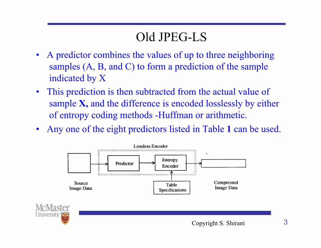
•  Any one of the eight predictors listed in Table 1 can be used.


Old JPEG-LS

•  If compression is performed in a non-real time environment all 8 modes of prediction can be tried and the one giving the most compression used.


CALIC •  CALIC: Context Adaptive Lossless Image Compression •  Uses both context and prediction of the pixel values •  Context: to obtain the distribution of the symbol being

encoded •  Prediction: use previous values of the sequence to obtain a

prediction of the value of the symbol being encoded •  In an image, a given pixel generally has a value close to one

of its neighbors •  Which neighbor has the closest value depends on the local

structure of the image


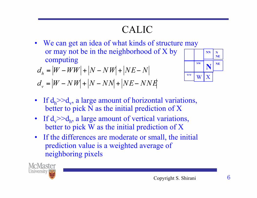
CALIC •  We can get an idea of what kinds of structure may

or may not be in the neighborhood of X by computing

•  If dh>>dv, a large amount of horizontal variations, better to pick N as the initial prediction of X

•  If dv>>dh, a large amount of vertical variations, better to pick W as the initial prediction of X

•  If the differences are moderate or small, the initial prediction value is a weighted average of neighboring pixels

NE

X

NNW

NNE

W

NN

WW


CALIC •  We refine this initial prediction using information about the

inter-relationship of the pixels in the neighborhood •  We quantify the information about the neighborhood by first

forming the vector [N, W, NW, NE, NN, WW, 2N-NN, 2W-WW]

•  We then compare each component of this vector with our initial prediction

•  If the value of the component is less than the prediction, we replace the value with a one, otherwise we replace it with a zero.


CALIC •  We also compute where is

the predicted value of N. •  The range of values for δ is divided into 4 intervals (the

combination of two consecutive interval in 8 context intervals explained in the next slide)

•  These 4 intervals along with 144 possibilities for the vector described above, 144x4=576 contexts for X.

•  Based on the context for the pixel, we find a value named offset and add it to the initial prediction of X.

•  The residual (difference between pixel value and the prediction) has to be encoded using its context.


CALIC •  The residual is mapped to [0,M-1] interval (original pixel

values are assumed to be between 0 and M-1. •  Context for encoding of residual is based on the range that δ

fall in: context 1 context 2

context 8

•  The residual is arithmetic coded using the context


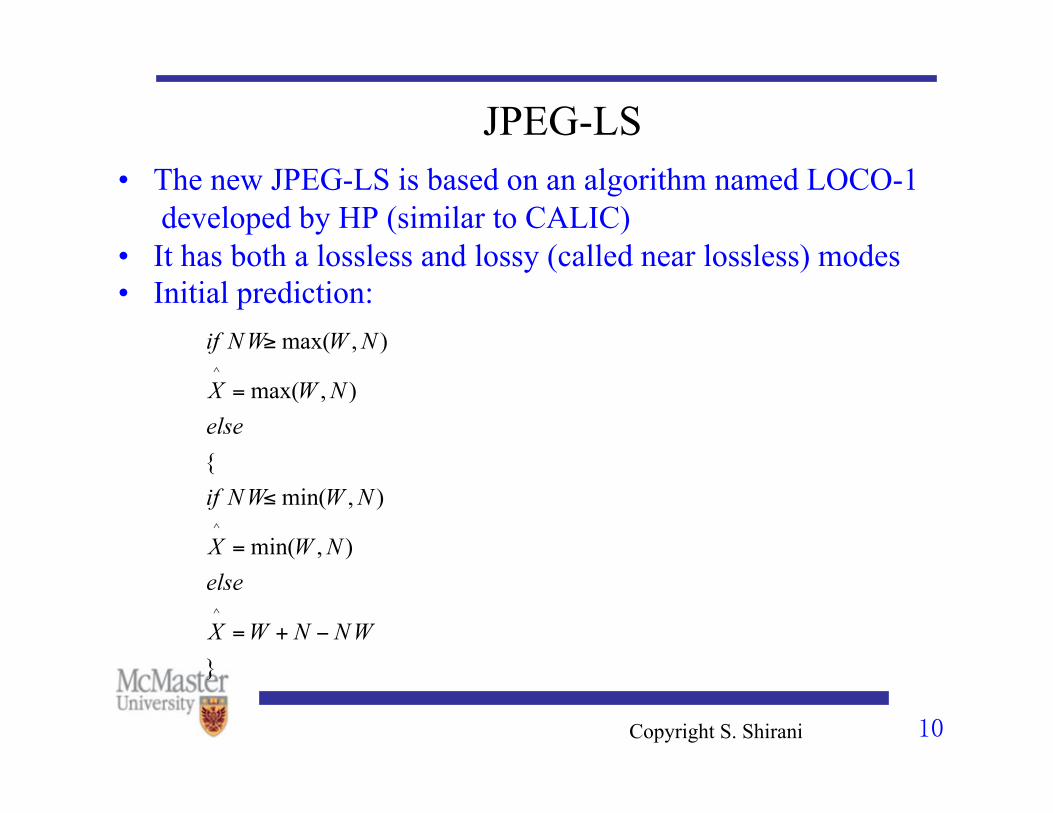
JPEG-LS •  The new JPEG-LS is based on an algorithm named LOCO-1

developed by HP (similar to CALIC) •  It has both a lossless and lossy (called near lossless) modes •  Initial prediction:


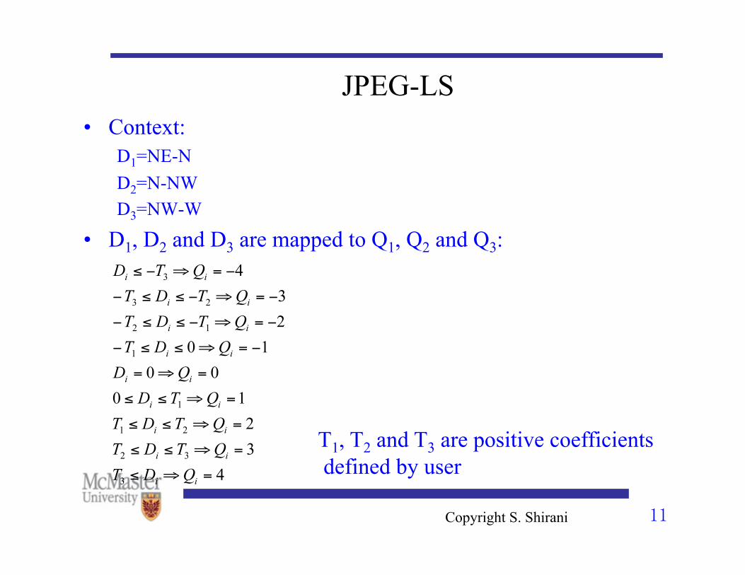
JPEG-LS •  Context:

D1=NE-N D2=N-NW D3=NW-W

•  D1, D2 and D3 are mapped to Q1, Q2 and Q3:

T1, T2 and T3 are positive coefficients defined by user


JPEG-LS •  Q1 and Q2 and Q3 define a context vector Q=(Q1, Q2 , Q3) •  Given 9 different values for each component, the context

vector can have 9x9x9=729 possible values •  The number of contexts is reduced by replacing any context

vector Q whose fist nonzero element is negative with –Q •  Whenever this happens a variable SIGN is set to -1, otherwise

it is set to 1 •  This reduces the number of context to 365 •  Q is then mapped to a number between 0 and 364. •  This number is used to find a correction value c[Q] •  c[Q] is multiplied by SIGN and added to initial prediction

error


JPEG-LS •  The prediction error rn is mapped into an interval that is the

same size as the range occupied by the original pixel values

•  Prediction errors are encoded based on Golomb codes.

(pixel values are between 0 and M-1)


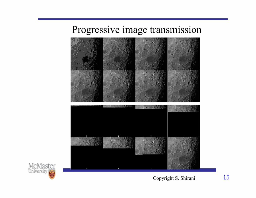
Progressive image transmission •  Last few years: a rapid increase in the amount of information

stored as images •  One issue: transmitting images to remote users •  A solution: send an approximation of each image (which does

not require too many bits) first •  If users find the image interesting they can request a further

refinement •  This approach is called progressive image transmission


Progressive image transmission


Facsimile Encoding •  CCITT has issued a number of recommendations for facsimile

encoding based on speed requirements •  CCITT classifies equipment for fax transmission into four

groups –  Group 1: 6 min for transmitting an A4 detailed in recommendation T2 –  Group 2: 3 min for transmitting an A4 detailed in recommendation T3 –  Group 3: 1 min for transmitting an A4 detailed in recommendation T4 –  Group 4: 1 min for transmitting an A4 detailed in recommendation T6

•  Run-length coding: coding the length of runs instead of coding individual values –  Exp: 190 white pixels, followed by 30 black, followed by 210 white –  Instead of coding 430 pixels individually, we code the sequence of

190,30, 210 along with an indication of the color of the first string


G3 •  Group 3: includes two coding schemes:

1.  1-D: coding of each line is performed independently of any other line 2.  2-D: coding of one line is performed using line to line correlation.

•  1-D coding: is a run-length coding scheme in which each line is represented as alternative white and black runs from left to right.

•  The first run is always a white run. So, if the first pixel is black, the white run has a length of zero.

•  Runs of different lengths occur with different probabilities, therefore they are coded using VLC (variable length codes).

•  CCITT uses Huffman coding


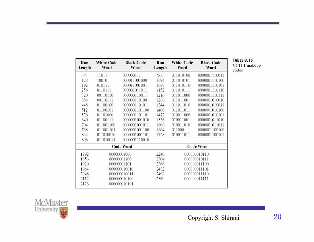
G3 •  The number of possible length of runs is huge and it is not

feasible to build a code book that large. •  The run length rl is expressed as:

–  rl=64*m+t t=0,1,..,63 m=1,2,…, 27

•  To represent rl, we use the corresponding codes for m and t. •  The code for t are called terminating codes and for m make-up

codes. •  If rl<63 only a terminating code is used •  Otherwise both a make-up code and a terminating code are

used •  A unique EOL (end of line) codeword 000000000001 is used

to terminate each line.


G3 •  2-D coding (modified READ=MR): rows of a facsimile image

are heavily correlated. Therefore it would be easier to code the transition points with reference to the previous line.

•  a0: the last pixel known to both encoder and decoder. At the beginning of encoding each line a0 refers to an imaginary white pixel to the left of actual pixel. While it is often a transition pixel it does not have to be.

•  a1: the first transition point to the right of a0. It has an opposite color of a0.

•  a2: the second transition pixel to the right of a0. Its color is opposite of a1.


G3 •  b1: the first transition pixel on the line above currently being

coded, to the right of a0 whose color is opposite of a0. •  b2: the first transition pixel to the right of b1 in the line above

the current line


G3 •  If b1 and b2 lie between a0 and a1 (pass mode): no transition

until b2. Then a0 moves to b2 and the coding continues. Transmitter transmits code 0001.

•  If a1 is detected before b2 –  If distance between a1 and b1 (number of pixels) is less than or equal

to 3, we send the location of a1 with respect to b1, move a0 to a1 and the coding continues (vertical mode)

–  If the distance between a1 and b1 is larger than 3, we go back to 1-D run length coding and encode the distance between a0 and a1 and a1 and a2 (horizontal mode) using run-length coding. a0 is moved to a2 and the coding continues.


G4 •  G4 encoding algorithm is identical to the 2-D encoding

algorithm in G3. •  G4 does not have a 1-D coding •  G4: modified modified READ (MMR)


Bi-level image compression standard JBIG

•  JBIG: joint bi-level image processing group •  Joint: ISO (international standards organization), IEC

(international electrotechnical commission) and CCITT (Consultative committee in international telephone and telegraph part of UN)

•  JBIG: a standard for the progressive encoding of bi-level images

•  JBIG: a progressive transmission algorithm and a lossless coding algorithm


Lossless coding algorithm •  Many bi-level images have a lot of local structure •  Exp: If pixels in the neighborhood of the pixel being coded

are mostly white, there is high probability that the pixel to be coded is also white

•  Skewed probabilities: ideal for arithmetic coding •  Each pixel based on its neighbors (context) is coded with a

different arithmetic coder •  These coders use the same computational engine, each with a

different set of probabilities •  JBIG: uses the pattern of pixels in the neighborhood (context)

of a pixel to decide which set of probabilities to use in encoding the pixel


Lossless coding algorithm •  If the context consists of 10 pixels there will be 1024 different

possible patterns •  JBIG coder uses 1024 to 4096 coders depending on whether a

low- or high- resolution layer is being coded

O O O O O O O A

O O X O

O

O

O O O O A

O O X


Progressive Transmission

•  In some applications we may not need to view an image in full resolution

•  Exp: the user is interested to see if there are any images in a page

•  In these applications a lower-resolution image is communicated to the user and the user will decide if a higher resolution image is necessary

•  A straightforward method for generating lower-resolution images is to replace every 2x2 block of pixels with the average of the four pixels

•  Does not work when two black and two white pixels


Progressive Transmission

•  JBIG uses a table-based method for resolution reduction •  The table is indexed by the neighboring pixels •  Lower-resolution layers can be used when coding higher

-resolution images •  JBIG uses the lower-resolution images as part of the context

for encoding the higher-resolution images •  In JBIG, 1024 arithmetic coders are a variation of the

arithmetic coder known as the QM coder


Progressive Transmission O

A O O O O X

O O

O O

O A O O

O O X O O

O O

O A O O

O O X O O

O O

O A O O

O O X O O

O O


JBIG2

•  JBIG2: allows lossy compression •  A large percentage of bi-level images consist of text on some

background and halftone images •  JBIG2 allows the encoder to select the compression technique

that would provide the best performance for the type of data •  Encoder divides the page to be compressed into three types of

regions: symbol regions, halftone regions, and generic regions –  Symbol regions: containing text –  Halftone regions: containing halftone images

•  Halftone: A reproduction of a grayscale image which uses dots of varying size or density to give the impression of areas of gray.

–  Generic regions: all regions not in the above two


Symbol region decoding

•  Symbol region coding is a dictionary-based procedure •  The compressed data contains the location a symbol to be

placed as well as the index to an entry in the symbol dictionary

•  As JBIG allows for lossy compression, the symbols do not have to exactly match the symbols in the original document


Generic decoding •  Two procedures are used to decode generic regions: generic

region decoding and generic refinement region decoding •  Generic region decoding: uses either the MMR technique

(used in G3 and G4 fax standards) or typical prediction. •  Typical prediction:

–  Observation: in a bi-level image a line is often identical to line above –  If a line is the same as the line above, a flag is set to 0 and the line is

not coded –  If this is not the case, flag is set to 1 and line is coded using the

method explained in JBIG

•  Generic refinement decoding: assumes a reference layer exists and decodes the data with reference to this layer


Halftone region decoding

•  Halftone region decoding is a dictionary-based procedure •  The compressed data contains the location of a halftone

region and an index to an entry in the halftone dictionary •  If lossy compression is used, the halftone patterns not have to

exactly match the patterns in the original document


MRC-T.44 •  Now a day, documents contain mutlicolored text as well as

color images. •  Recommendation T.44 for Mixed Raster Content (MRC)

takes the approach of separating the document into elements that can be compressed using available techniques.

•  T.44 divides a page into slices where width of the slice is equal to the width of the entire page

•  The height is variable •  In the base mode, each slice is represented by three layers:

background, foreground and mask •  Layers are used to represent three basic data types: color

images, bi-level data and multi-level data


•  The multilevel image data is put in the background layer, the mask and foreground layers are used to represent the bi-level and multi-level nonimage data

Lossless Image Compression - McMaster Universityshirani/multi08/losslessimage.pdf · • CALIC:...

Documents

Transcript of Lossless Image Compression - McMaster Universityshirani/multi08/losslessimage.pdf · • CALIC:...