Loss Function Based Ranking in Two-Stage,

Hierarchical Models

Rongheng Lin1, Thomas A. Louis, Susan M. Paddock, Greg Ridgeway2

Oct 26, 2004

1Address for correspondence: Department of Biostatistics, Johns Hopkins Bloomberg School of PublicHealth, 615 N. Wolfe St., Baltimore MD 21205, U.S.A. E-mail:rlin@jhsph.edu

2Rongheng Lin is Ph.D candidate and Thomas A. Louis is Professor, Department of Biostatistics, JohnsHopkins Bloomberg School of Public Health, Baltimore, MD 21205, U.S.A. Susan M. Paddock is Full Statis-tician and Greg Ridgeway is Full Statistician, RAND, Santa Monica, CA 90401, U.S.A. This work wassupported by grant 1-R01-DK61662 from U.S. NIH National Institute of Diabetes, Digestive and KidneyDiseases.

Loss Function Based Ranking in Two-Stage,Hierarchical Models

Abstract

Several authors have studied the performance of optimal, squared error loss (SEL) estimated

ranks. Though these are effective, in many applications interest focuses on identifying the

relatively good (e.g., in the upper 10%) or relatively poor performers. We construct loss

functions that address this goal and evaluate candidate rank estimates, some of which opti-

mize specific loss functions. We study performance for a fully parametric hierarchical model

with a Gaussian prior and Gaussian sampling distributions, evaluating performance for sev-

eral loss functions. Results show that though SEL-optimal ranks and percentiles do not

specifically focus on classifying with respect to a percentile cut point, they perform very

well over a broad range of loss functions. We compare inferences produced by the candidate

estimates using data from The Community Tracking Study.

KEY WORDS: Bayesian Methods, Percentiles, League Tables, Decision Theory

1 Introduction

The prevalence of performance evaluations of health services providers using ranks or per-

centiles (Goldstein and Spiegelhalter 1996; Christiansen and Morris 1997; McClellan and

Staiger 1999; Landrum et al. 2000; Normand et al. 1997), using post-marketing information

to evaluate drug side-effects (DuMouchel 1999), ranking geographic regions using disease

incidence, (Devine and Louis 1994; Devine et al. 1994; Conlon and Louis 1999) and ranking

teachers and schools (i.e., value added modeling) burgeons. Goals of such investigations

include valid and efficient estimation of population parameters such as the average perfor-

mance (over clinics, physicians, health service regions or other “units of analysis”), estimation

of between-unit variation (variance components), and unit-specific evaluations. These lat-

ter include estimating unit specific performance (point estimates and confidence intervals),

computing the probability that a unit’s true, underlying performance is in an “acceptable”

(or unacceptable) region, ranking/percentiling units as input to profiling and league tables

(Goldstein and Spiegelhalter 1996), identification of excellent and poor performers.

1

Bayesian models are very effective in structuring these assessments. Inferences always depend

on the posterior distribution, but how the posterior is used should depend on inferential goals.

As Shen and Louis (1998) show and Gelman and Price (1999) present in detail, no single

set of estimates can effectively address the multiple goals. For example, the histogram of

maximum likelihood estimates (MLEs) is always over-dispersed relative to the histogram of

the true random effects. In a Bayesian setting, the histogram of posterior means (PMs) is

always under-dispersed. Therefore, when inferences address non-standard goals, they are

best guided by a loss function. In this vein, Shen and Louis (1998) used squared-error loss

(SEL) to estimate the cumulative distribution function of unit-specific parameters in a two

stage hierarchical model and to estimate the ranks of these parameters. They show that

ranks estimated in this way outperform competitors.

As the following authors show, even optimal percentile estimates can perform quite poorly

in most real-world settings. Lockwood and co-authors (Lockwood, Louis, and McCaffrey

2002) present simulation-based evaluations of SEL-based optimal percentiles with application

to comparing performance of teachers and schools (value added modeling in educational

assessment), Liu et al. (2004) provide evaluations with specific reference to ranking dialysis

centers with respect to standardized mortality ratios, Goldstein and Spiegelhalter (1996)

compute “league tables” for schools and surgeons.

SEL applies the same distance function to all (estimated, true) percentile pairs, but in many

applications interest focuses on identifying the relatively good (e.g., in the upper 10%) or

relatively poor performers. For example, quality improvement initiatives should be targeted

at health care providers that truly perform poorly; environmental assessments should be tar-

geted at the truly high incidence locations; genes with the truly highest differential expression

should be the ones to generate hypotheses. In this report we construct loss functions that

address such goals and evaluate candidate rank (percentile) estimates, some of which opti-

mize specific loss functions. We study performance for a fully parametric hierarchical model

with a Gaussian prior and Gaussian sampling distributions (both with constant and unit-

specific sampling variance). We evaluate performance for the loss function used to generate

(or motivate) the ranks and for other candidate loss functions, thereby evaluating both the

2

performance of the optimal or loss function tuned estimates and robustness to assumptions

and goals.

Results show that though SEL-optimal ranks and percentiles do not specifically focus on

classifying with respect to a percentile cut point, they perform very well over a broad range

of loss functions. We compare inferences produced by the candidate estimates using data

from The Community Tracking Study (Kemper et al. 1996; Center for Studying Health

System Change 2003).

2 The two-stage, Bayesian hierarchical model

We consider a two-stage model with iid sampling from a known prior (G with density g)

and possibly different sampling distributions:

θ1, . . . , θK iid G(θk)

Yk | θk ∼ fk(Yk | θk) (1)

θk | Yk ind gk(θk | Yk) =fk(Yk | θk)g(θk)∫fk(Yk | u)g(u)du

.

Note that the fk can depend on k. This model can be generalized to allow a regression

structure in the prior and can be extended to three stages with a hyper-prior to structure

“Bayes empirical Bayes” (Conlon and Louis 1999; Louis and Shen 1999; Carlin and Louis

2000).

2.1 Loss functions and decisions

Let θ = (θ1, . . . , θK) and Y = (Y1, . . . , YK). For a decision rule a(Y) and loss function

L(θ, a), the optimal Bayesian procedure (the optimal a(Y)) minimizes the posterior and

preposterior Bayes risks,

RG(a(Y),Y) = Eθ|Y[L(θ, a(Y) | Y]

RG(a) = EY[RG(a(Y),Y)].

3

For any a(Y) we can compute the frequentist risk:

R(θ, a(·)) = EY|θ[L(θ, a(Y)) | θ].

3 Ranking

In general, the optimal ranks for the θk are neither the ranks of the observed data nor the

ranks of their posterior means. Laird and Louis (1989) structure estimation by representing

the ranks as,

Rk(θ) = rank(θk) =K∑

j=1

I{θk≥θj} (2)

with the smallest θ having rank 1.

3.1 Squared-error loss

This is the most common estimation loss function. It is optimized by the posterior mean of

the target parameter. For example, with the unit-specific θs as the target, the loss function

is L(θ, a) = (θ − a)2 and θpmk = E(θk | Y). To produce SEL-optimal ranks, minimize the

squared error loss (SEL) for them,

L = L(Rest, R(θ)) =1

K

∑

k

(Restk −Rk(θ))2, (3)

where Restk are generic estimates. L is optimized by the posterior means,

Rk(Y) = EG[Rk(θ) | Y] =K∑

j=1

PG[θk ≥ θj | Y].

The Rk are shrunk towards the mid-rank (K + 1)/2, and generally the Rk are not integers

(see Shen and Louis 1998). Generally we want integer ranks and use

Rk(Y) = rank(Rk(Y)), (4)

which are the optimal, integer estimates. See Section A.1 for additional details on the SEL

approach.

In the sequel, generally we drop dependency on θ and omit conditioning on Y. For example,

Rk stands for Rk(θ) and Rk stands for Rk(Y). Furthermore, use of the ranks facilitates

4

notation in mathematical proofs, but in many applications percentiles,

Pk = Rk/(K + 1) (5)

are used, e.g. Pk = Rk/(K + 1). Also, percentiles have the advantage of normalizing with

respect to the number of units K. For example, Lockwood et al. (2002) show that mean

square error (MSE) for percentiles rapidly converges to a function that does not depend

on K and their use similarly standardizes our new loss functions. We use both ranks and

percentiles with the choice depending on presentation clarity.

4 Upper 100(1− γ)% loss functions

When posterior distributions are not stochastically ordered, SEL (L)-optimal percentiles (the

Pk) outperform ranking the θpmk and substantially outperform ranking the MLEs. However,

L evaluates general performance without specific attention to identifying the relatively good

or relatively poor performers. To attend to this goal, for 0 < γ < 1 we investigate loss

functions that focus on identifying the upper 100(1− γ)% of the units (identification of the

lower group is similar) and may also include a distance penalty. For notational clarity we

assume that γK is an integer, so γ(K + 1) is not an integer and in the following it is not

necessary to make the distinction between > and ≥ (< and ≤).

4.1 Summed, unit-specific loss functions

To structure loss functions, for 0 < γ < 1, let

ABk(γ, Pk, Pestk ) = I{Pk>γ, P est

k <γ} = I{Rk>γ(K+1), Restk <γ(K+1)} (6)

BAk(γ, Pk, Pestk ) = I{Pk<γ, P est

k >γ} = I{Rk<γ(K+1), Restk >γ(K+1)},

ABk and BAk indicate the two possible modes of misclassification of the percentiles. ABk

indicates that the true percentile is above the cutoff, and therefore unit k should be flagged;

however, the estimated percentile is below the cutoff. Similarly BAk indicates that the true

percentile is below the cutoff while the estimated percentile is above it.

5

For p, q, c > 0 define,

L(γ, p, q, c) =1

K

∑

k

{|γ − P estk |pABk(γ, Pk, P

estk ) + c|P est

k − γ|qBAk(γ, Pk, Pestk )}

L†(γ, p, q, c) =1

K

∑

k

{|Pk − γ|pABk(γ, Pk, Pestk ) + c|γ − Pk|qBAk(γ, Pk, P

estk )} (7)

L‡(γ, p, q, c) =1

K

∑

k

{|Pk − P estk |pABk(γ, Pk, P

estk ) + c|P est

k − Pk|qBAk(γ, Pk, Pestk )}

L0/1(γ) =

∑k{ABk(γ, Pk, P

estk ) + BAk(γ, Pk, P

estk )}

K= 2

∑k ABk(γ, Pk, P

estk )

K

=#(misclassifications)

K= L(γ, 0, 0, 1) = L†(γ, 0, 0, 1) = L‡(γ, 0, 0, 1)

Lall(γ) = 0 or 1 according as all classifications are correct or at least 1 is incorrect

= 1−∏

k

{1− ABk(γ, Pk, Pestk )}{1−BAk(γ, Pk, P

estk )}

Lall(γ) is “all or nothing,” with no penalty if all (P estk , Pk) pairs are on the same side of the cut

point and penalizing by 1 if there are any discrepancies. The other loss functions confer no

penalty if an estimated and true unit-specific percentile pair (P estk , Pk) are either both above

or both below the γ cut point. If they are on different sides of the cut point, the loss functions

penalize by an amount that depends on the distance of either the estimated or the true

percentile from the cut point or on the distance between the true and estimated percentiles.

The parameters p and q adjust the intensity of the two penalties; p 6= q and c 6= 1 allow

for differential penalties for the two kinds of misclassification. L0/1(γ) counts the number of

discrepancies and is equivalent to the preceding three functions with p = q = 0, c = 1.

Several of our mathematical results apply to the general form of the loss functions (7), but

our simulations evaluate them for p = q = 2, c = 1. The foregoing simplify to:

L(γ) =1

K

∑

k

(γ − P estk )2{ABk(γ, Pk, P

estk ) + BAk(γ, Pk, P

estk )}

L†(γ) =1

K

∑

k

(Pk − γ)2{ABk(γ, Pk, Pestk ) + BAk(γ, Pk, P

estk )} (8)

L‡(γ) =1

K

∑

k

(Pk − P estk )2{ABk(γ, Pk, P

estk ) + BAk(γ, Pk, P

estk )}.

6

4.2 A convex combination loss function

Though the loss functions (7) and (8) are most relevant in applications, the convex combi-

nation loss,

Lw0/1(γ) = (1− w)L0/1(γ) + wL (9)

is a possible alternative to L‡. (Convex combination losses derived from L and L† are less

interesting in that once the (above γ)/(below γ) groups are determined, no further control

is possible). Once the (above γ)/(below γ) groups have been specified, risk is controlled

by constrained optimization of L. We do not report simulations for Lw0/1(γ), but use it to

motivate the estimator ˆPk(γ) defined in Section 5.5.

5 Optimizers and other candidate estimates

In addition to Pk which minimizes L (SEL, see equation (4)), we consider an estimator that

optimizes both L0/1 and L and one that is motivated by Lw0/1. Note that when the posteriors

are stochastically ordered the Pk are optimal for broad class of loss functions.

5.1 Optimizing Lall

Optimization requires finding the subscripts (k1, k2, . . . , k(1−γ)K) that maximize:

pr({Rk1 , Rk2 , . . . , Rk(1−γ)K} = {γK, γK + 1, . . . , K}).

Finding this optimal subset requires the full joint distribution of the ranks and evaluating all

possible (1−γ)K-element subsets. Even if the joint distribution is available, the optimization

is infeasible unless

(K

[γK]

)is small.

5.2 Optimizing L0/1

Let,pk` = pr(Rk = ` | Y)

πk(γ) = pr(Rk ≥ γ(K + 1) | Y) = pr(Pk ≥ γ | Y) =K∑

`=[γK]+1

pk` (10)

Rk(γ) = rank(πk(γ)); Pk(γ) = Rk(γ)/(K + 1) (11)

7

Theorem 1. The Pk(γ) optimize L0/1, but not uniquely.(L0/1 does not require optimal

ordering, only optimal categorization above and below the cut point. Other loss functions

provide additional structure and resolution.)

Proof. Rewrite the loss function as a function of the number of coordinates not classified in

the top (1− γ)K but that should have been. Then, L0/1 = 1K

(K − |A ∩ T |), where A is the

classified set and T is the true set of (1− γ)K numbers. We need to maximize the expected

number of correctly classified coordinates:

E|A ∩ T | = E∑

I(θi ∈ A ∩ T ) = E∑

I(θi ∈ A)I(θi ∈ T )

= E∑

θi∈A

I(θi ∈ T ) =∑

θi∈A

pr(θi ∈ T ).

So, to optimize L0/1, for each θi calculate pr(θi ∈ T ), rank these probabilities and select

the largest (1 − γ)K of them. That is to calculate pr(θk ∈ T ) =∑K

`=(1−γ)K pk` = πk(γ).

Therefore, ordering by the πk(γ) creates the optimal “(above γ)/(below γ) ” groups.

This computation can be difficult and time-consuming, but is Monte Carlo implementable.

We note that here the optimizer Pk(γ) produced by πk(γ) is in the similar spirt of the

ranking proposed by Normand et al. (1997), which suggests to use Pr(θk > c) to compare

the performance.

5.3 Optimizing L

Theorem 2. The Pk(γ) optimize L.

The proof, in Section A.2, shows that the Pk(γ) are optimal for more general loss functions

with the distance penalties |γ−P estk |p and c|P est

k −γ|q replaced by any nondecreasing functions

of |γ − P estk |.

5.4 Optimizing L†

We have not identified a general representation or algorithm for the optimal ranks. However,

Section A.3 develops an optimization procedure for the case p = q = 2,−∞ < c < ∞. Note

8

that as for L0/1, performance depends only on optimal allocation into the (above γ)/(below γ)

groups. Additional criteria are needed to specify the within-group order.

5.5 Optimizing L‡

We have not identified a general representation or algorithm for the optimal ranks. However,

Section A.4 develops a helpful relation. The estimator ˆPk(γ), motivated by loss function (9),

is very effective though not optimal for L‡.

Definition of ˆPk(γ): Use the Pk(γ) to determine which coordinates comprise the (above γ)/(below γ)

percentile groups. Then, within each percentile group order the coordinates by Pk.

Since the (above γ)/(below γ) groups are formed by Pk(γ), ˆPk(γ) also minimizes L0/1. In

addition, we have the following.

Theorem 3. For any (above γ)/(below γ) grouping, ordering within the groups by the Pk

produces the constrained minimum for L.

Proof. To see this, without loss of generality, assume that coordinates (1, . . . , γK) are in the

(below γ) group and (γK + 1, . . . , K) are in the (above γ) group. Similar to Section A.1,

E∑

k

(Rest

k −Rk

)2=

∑

k

V (Rk) +∑

k

(Rest

k −Rk

)2

Nothing can be done to reduce the variance terms and the summed squared bias partitions

into,∑

k

(Rest

k −Rk

)2=

γK∑

k=1

(Rest

k −Rk

)2+

K∑

k=γK+1

(Rest

k −Rk

)2

which must be minimized subject to the constraints that (Rest1 , . . . , Rest

γK) ∈ {1, . . . , γK} and

(RestγK+1, . . . , R

estK ) ∈ {γK + 1, . . . , K}. We deal only with the (below γ) group; the (above

γ) group is similar. Again, without loss of generality assume that R1 < R2 < . . . < RγK

and compare SEL for Restk = rank(Rk) = k, k = 1, . . . , γK to any other assignment. It is

straightforward to show that switching any pair that does not follow the Rk order to follow

9

that order reduces SEL. Iterating this and noting that the Rk = rank(Rk) produces the

result.

Consequence: For the convex combination loss function Lw0/1(γ) (formula 9), it is straight-

forward to show that there exists a w∗ > 0 such that for all w ≤ w∗,ˆPk(γ) is optimal

(motivating it as a candidate estimator). Similarly, there exists a w∗ < 1 such that for all

w ≥ w∗, Pk is optimal (broadening its potential use).

5.6 Relations among estimators

Let ν = [γK] and define

R∗k(ν) =

K(K + 1)

2(K − ν + 1)pr(Rk ≥ ν) =

K(K + 1)

2(K − ν + 1)πk(γ).

The rank of the R∗k(ν) is same as the rank of the πk(γ) and so each generate the Rk(γ). Note

that,∑

k

K(K + 1)

2(K − ν + 1)πk(γ) =

∑

k

R∗k(ν) =

K(K + 1)

2=

∑

k

Rk.

Theorem 4. Rk is a linear combination of the R∗k(ν) with respect to ν and so for any

convex loss function Rk outperforms R∗k(ν) for at least one value of ν = 1, . . . , K. For

SEL, Rk dominates for all ν. As shown in Section A.1, the Rk = rank(Rk) also dominate

rank(R∗k(ν)) for all ν.

Proof. Recall that for a positive, discrete random variable the expected value can be com-

puted as the sum of (1 - cdf), so

Rk =K∑

ν=1

νpr[Rk = ν] =K∑

ν=1

pr[Rk ≥ ν] =K∑

ν=1

πk

(ν

K + 1

)(12)

=K∑

ν=1

2(K − ν + 1)

K(K + 1)

K(K + 1)

2(K − ν + 1)pr[Rk ≥ ν]

=K∑

ν=1

2(K − ν + 1)

K(K + 1)R∗

k(ν)

10

Relation (12) can be used to show that when the posterior distributions are stochastically

ordered, Rk ≡ Rk(γ). In this case, for all γ the πk(γ) have the same order and so the Rk

inherit this order. More generally, if the posterior distributions gk(t | Yk) are stochastically

ordered (the Gk(t | Yk) never cross), then for a broad class of loss functions (including many

that we consider) the Rk are optimal.

6 Simulation Scenarios and Results6.1 Scenarios

6.1.1 Gaussian-Gaussian model

We evaluate estimators for the Gaussian/Gaussian, two-stage model with a Gaussian prior

and Gaussian sampling distributions that may have different variances. Without loss of

generality we assume that the prior mean µ = 0 and the prior variance τ 2 = 1. Specifically,

θk iid N(0, 1)

Yk|θk ∼ N(θk, σ2k)

gk(θk | Yk) ∼ N(θpm

k , (1−Bk)σ2k

)

θpmk = (1−Bk)Yk

Bk = σ2k/(σ

2k + 1).

The variances {σ2k} form an ordered, geometric sequence with specified ratio of geometric

mean to τ 2. Sine we use τ 2 = 1 in our prior, this ratio is then equal to the geometric mean

of the variance sequence gmv = GM(σ21, . . . , σ

2K). Furthermore, we use rls = σ2

K/σ21, the

ratio of the largest σ2k to the smallest as an indicator of range of variance.

Each result is based on K = 200 with nrep = 2000 simulation replications. We compute

the pk` (needed to compute Pk(γ)) using an independent sample Monte Carlo with n = 2000

draws. All simulations are for loss functions with p = q = 2; c = 1.

11

6.1.2 Mixture model

We consider the situation that θ comes from a two-component mixture of Gaussian distri-

bution which has mean 0 and variance 1:

θkiid∼ (1− ε)N

(−ε∆

A,

1

A2

)+ εN

((1− ε)∆

A,

ξ2

A2

)

where

A2 = A2(ε, ∆, ξ) = (1− ε) + εξ2 + ε(1− ε)∆2

This form comes from standardizing θiid∼ (1−ε)N(0, 1)+εN(∆, ξ2) to mean 0 and variance 1.

We then calculate the preposterior risk for estimators in percentiles in two way: assuming

that we know exactly θ′s are from mixture prior (part II of the table); incorrectly assuming

that θ′s are from N(0,1) (part III of the table). Like the Gaussian-Gaussian scenario, we

selected K = 200, n = 2000, nrep = 2000; p = q = 2; c = 1. We use several sets of extra

parameters values and here only present the results for ε = .1, ∆ = 3.40, ξ2 = .25, γ = .9.

6.2 Results

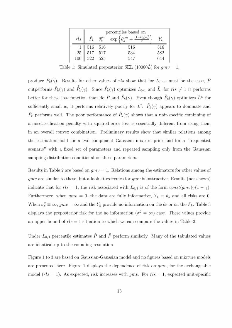
Table 1 documents SEL (L) performance for Pk, the optimal estimator, for percentiled Yk,

percentiled θpmk and percentiled exp

{θpm

k +(1−Bk)σ2

k

2

}(the posterior mean of eθk), this latter

to assess performance for a monotone, non-linear transform of the target parameters. For

rls = 1, the posterior distributions are stochastically ordered and the four sets of percentiles

are identical. As rls increases, performance of Yk-derived percentiles degrades, those based

on the θpmk are quite competitive with Pk but performance for percentiles based on the

posterior mean of eθk degrades. Results show that though the posterior mean can perform

well for some models and target parameters, in general it is not competitive. We do not

include these estimates in subsequent evaluations.

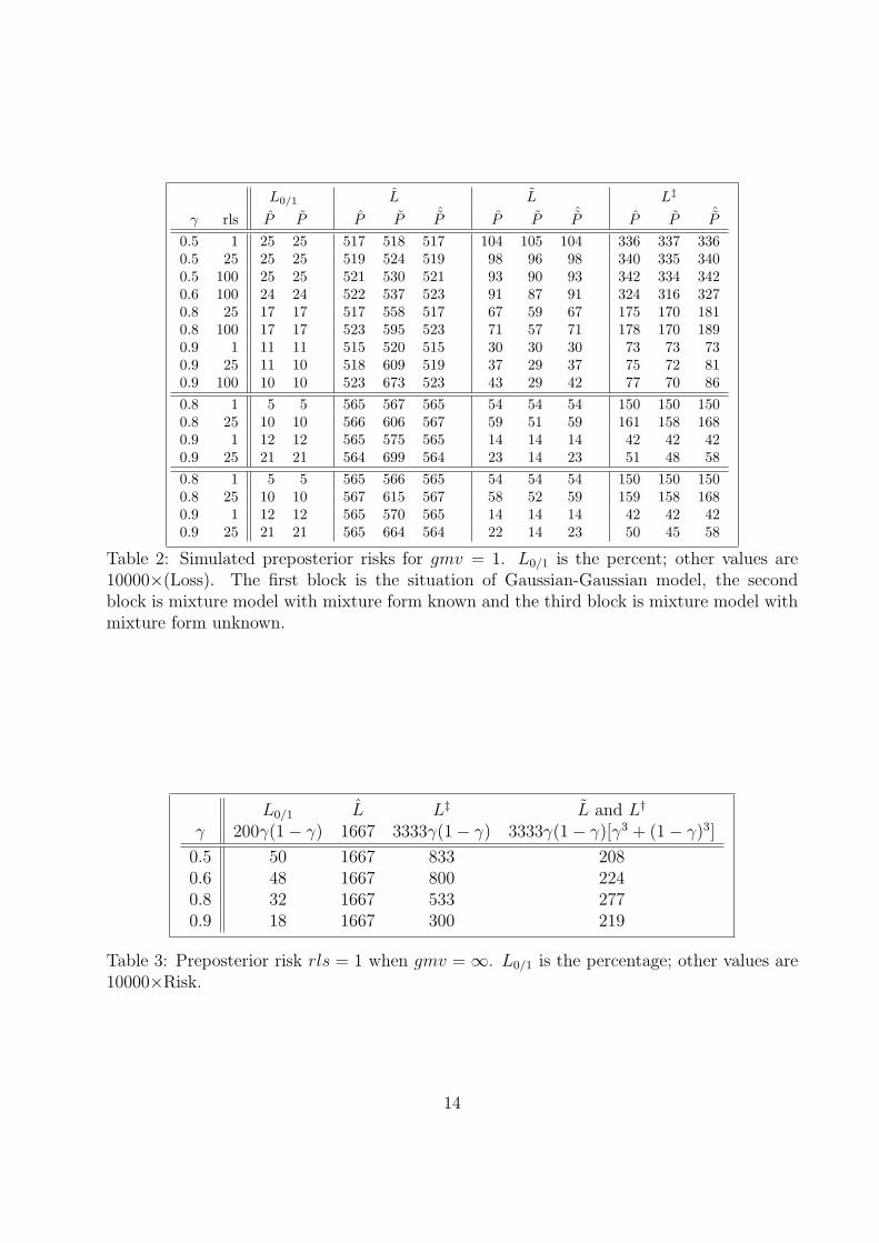
Table 2 reports results for the remaining competitors. Again, when rls = 1, Pk(γ) ≡ Pk ≡ˆPk(γ) and so the SEL results in the first and seventh rows show the small residual variation

in the simulation and the Monte Carlo evaluation of the posterior distribution needed to

12

percentiles based on

rls Pk θpmk exp

{θpm

k +(1−Bk)σ2

k

2

}Yk

1 516 516 516 51625 517 517 534 582

100 522 525 547 644

Table 1: Simulated preposterior SEL (10000L) for gmv = 1.

produce Pk(γ). Results for other values of rls show that for L, as must be the case, P

outperforms Pk(γ) and ˆPk(γ). Since Pk(γ) optimizes L0/1 and L, for rls 6= 1 it performs

better for these loss function than do P and ˆPk(γ). Even though ˆPk(γ) optimizes Lw for

sufficiently small w, it performs relatively poorly for L‡. Pk(γ) appears to dominate and

Pk performs well. The poor performance of ˆPk(γ) shows that a unit-specific combining of

a misclassification penalty with squared-error loss is essentially different from using them

in an overall convex combination. Preliminary results show that similar relations among

the estimators hold for a two component Gaussian mixture prior and for a “frequentist

scenario” with a fixed set of parameters and repeated sampling only from the Gaussian

sampling distribution conditional on these parameters.

Results in Table 2 are based on gmv = 1. Relations among the estimators for other values of

gmv are similar to these, but a look at extremes for gmv is instructive. Results (not shown)

indicate that for rls = 1, the risk associated with L0/1 is of the form const(gmv)γ(1 − γ).

Furthermore, when gmv = 0, the data are fully informative, Yk ≡ θk and all risks are 0.

When σ2k ≡ ∞, gmv = ∞ and the Yk provide no information on the θs or on the Pk. Table 3

displays the preposterior risk for the no information (σ2 = ∞) case. These values provide

an upper bound of rls = 1 situation to which we can compare the values in Table 2.

Under L0/1 percentile estimates P and P perform similarly. Many of the tabulated values

are identical up to the rounding resolution.

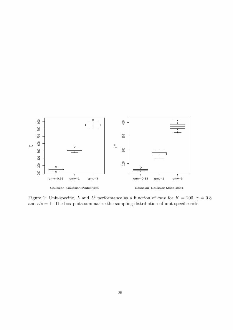
Figure 1 to 3 are based on Gaussian-Gaussian model and no figures based on mixture models

are presented here. Figure 1 displays the dependence of risk on gmv, for the exchangeable

model (rls = 1). As expected, risk increases with gmv. For rls = 1, expected unit-specific

13

L0/1 L L L‡

γ rls P P P P ˆP P P ˆP P P ˆP0.5 1 25 25 517 518 517 104 105 104 336 337 3360.5 25 25 25 519 524 519 98 96 98 340 335 3400.5 100 25 25 521 530 521 93 90 93 342 334 3420.6 100 24 24 522 537 523 91 87 91 324 316 3270.8 25 17 17 517 558 517 67 59 67 175 170 1810.8 100 17 17 523 595 523 71 57 71 178 170 1890.9 1 11 11 515 520 515 30 30 30 73 73 730.9 25 11 10 518 609 519 37 29 37 75 72 810.9 100 10 10 523 673 523 43 29 42 77 70 860.8 1 5 5 565 567 565 54 54 54 150 150 1500.8 25 10 10 566 606 567 59 51 59 161 158 1680.9 1 12 12 565 575 565 14 14 14 42 42 420.9 25 21 21 564 699 564 23 14 23 51 48 580.8 1 5 5 565 566 565 54 54 54 150 150 1500.8 25 10 10 567 615 567 58 52 59 159 158 1680.9 1 12 12 565 570 565 14 14 14 42 42 420.9 25 21 21 565 664 564 22 14 23 50 45 58

Table 2: Simulated preposterior risks for gmv = 1. L0/1 is the percent; other values are10000×(Loss). The first block is the situation of Gaussian-Gaussian model, the secondblock is mixture model with mixture form known and the third block is mixture model withmixture form unknown.

L0/1 L L‡ L and L†

γ 200γ(1− γ) 1667 3333γ(1− γ) 3333γ(1− γ)[γ3 + (1− γ)3]

0.5 50 1667 833 2080.6 48 1667 800 2240.8 32 1667 533 2770.9 18 1667 300 219

Table 3: Preposterior risk rls = 1 when gmv = ∞. L0/1 is the percentage; other values are10000×Risk.

14

loss equals the overall average risk and so the box plots summarize the sampling distribution

of unit-specific risk.

6.2.1 Unit-specific performance

When rls = 1, pre-posterior risk is the same for all units. However, when rls > 1, the

σ2k form a geometric sequence and preposterior risk depends on the unit. We have not

pursued mathematical results for this non-exchangeable situation, but study it by simulation.

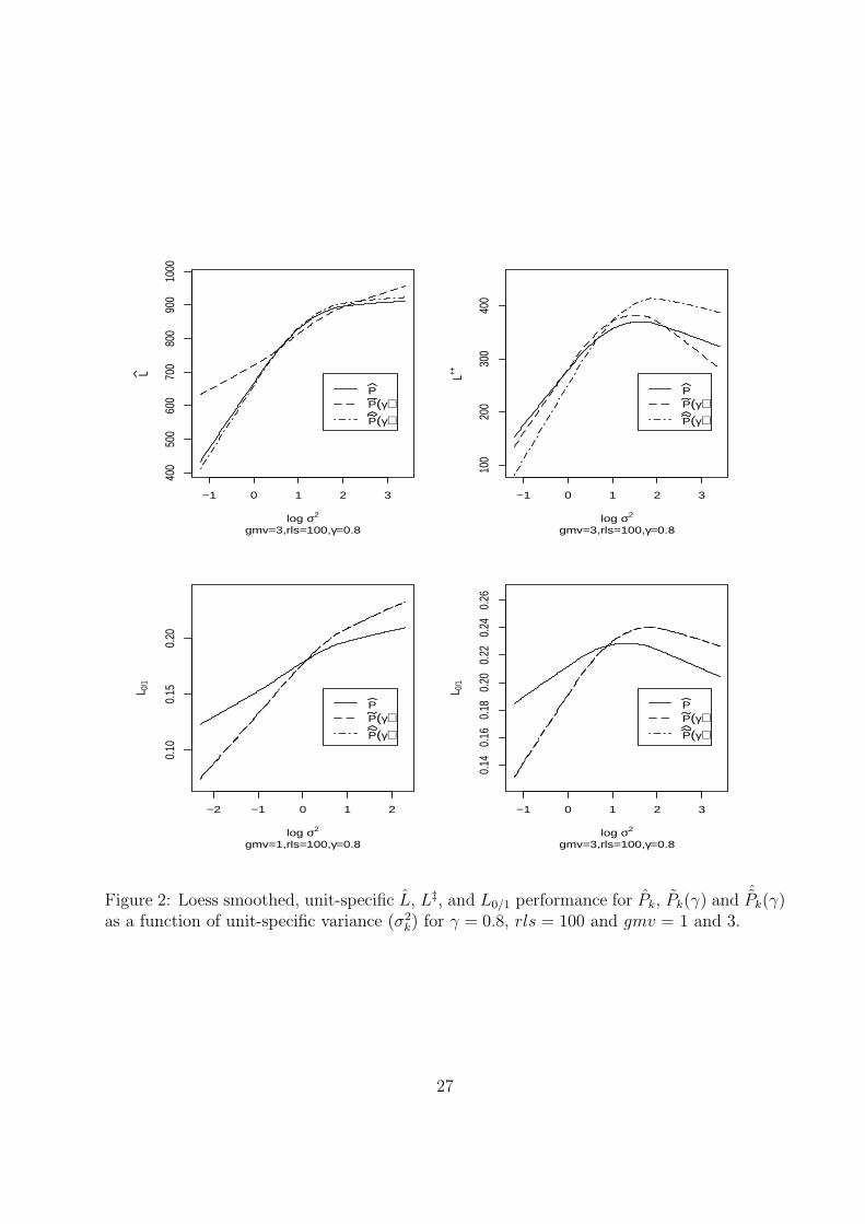
Figure 2 displays loess smoothed performance of Pk, Pk(γ) and ˆPk(γ) for L0/1, L and L‡ as

a function of unit-specific variance for gmv = 1 and 3, rls = 100 and γ = 0.8. The plots

for L (gmv = 3) and for L0/1 (gmv = 1) correspond to intuition in that risk increases with

increasing unit-specific variance. However, in the displays for L0/1 (gmv = 1) and for L‡,

for all estimators as a function of σ2k the risk increases and then decreases. Similar patterns

emerge for other values of γ, gmv and rls with the presence of a downturn depending on the

proximity of γ to 0.5 and rls or gmv being sufficiently large.

These results appear anomalous; however they can be explained. If γ near 1 (or equivalently,

near 0) and if the σ2k differ sufficiently (rls > 1), estimates for the high variance units perform

better than for those with mid-level variance. This relation is due to improved classification

into the (above γ)/(below γ) groups, with the improvement due to the substantial shrinkage

of the percentile estimates for high-variance units towards 50%. For example, with γ = 0.8, a

priori 80% of the percentiles should be below 0.8. Estimated percentiles for the high variance

units are essentially guaranteed to be below 0.8 and so the classification error for the large-

variance units converges to 20% as rls →∞. Low variance units have small misclassification

probabilities. Percentiles for units with moderate variances are not shrunken sufficiently

toward 0.5 to produce a low L0/1.

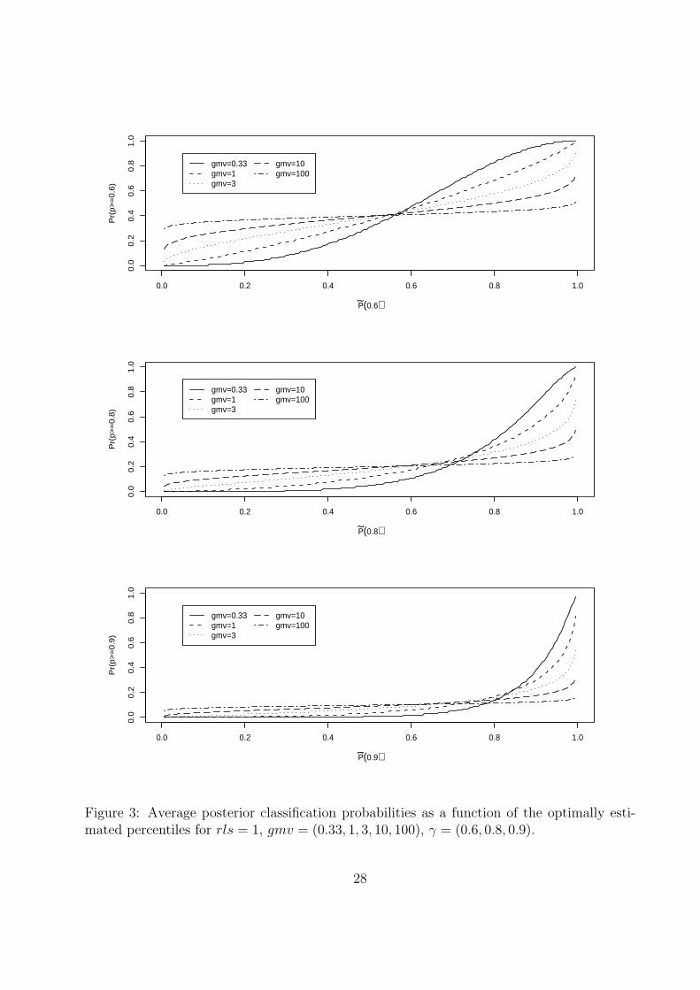
6.2.2 Classification performance

As shown in the foregoing tables and by Liu et al. (2004) and Lockwood et al. (2002), even

the optimal ranks and percentiles can perform poorly unless the data are very informative.

Figure 3 displays average posterior classification probabilities as a function of the optimally

estimated percentile for gmv = 0.33, 1, 10, 100 and γ = 0.6, 0.8, 0.9, when rls = 1. The

15

γ = 0.8 panel is typical. Discrimination improves with decreasing gmv, but even when

gmv = 0.33 (the σk are 1/3 of the prior variance), for a unit with Pk(0.8) = 0.8, the model-

based, posterior probability that Pk > 0.8 is only 0.42. For this probability to exceed 0.95

(i.e., to be reasonably certain that Pk > 0.80) requires that Pk(0.8) > 0.97. It can be shown

that as gmv → ∞ the plots converge to a horizontal line at (1 − γ) and that as gmv → 0

the plots converge to a step function jumps from 0 to 1 at γ.

7 Analysis of the Community Tracking Study

We compare Pk, Pk(γ) and ˆPk(γ) using income data from The Community Tracking Study

(CTS). CTS is a national survey designed to monitor changes in the health care system and

their effects on insurance coverage, access to care, service use and delivery, cost, and quality

of care (Kemper et al. 1996). Since 1996, data have been collected every two years on the 60

communities in the 48 contiguous states enrolled into the study. A total of 56,343 persons

were sampled as part of the 60 site samples. A random subset of 12 of these sites are selected

to be “high-intensity” sites that could be studied individually in greater detail. We examine

data from the third wave of the study, which was conducted during 2000-2001 (Center for

Studying Health System Change 2003).

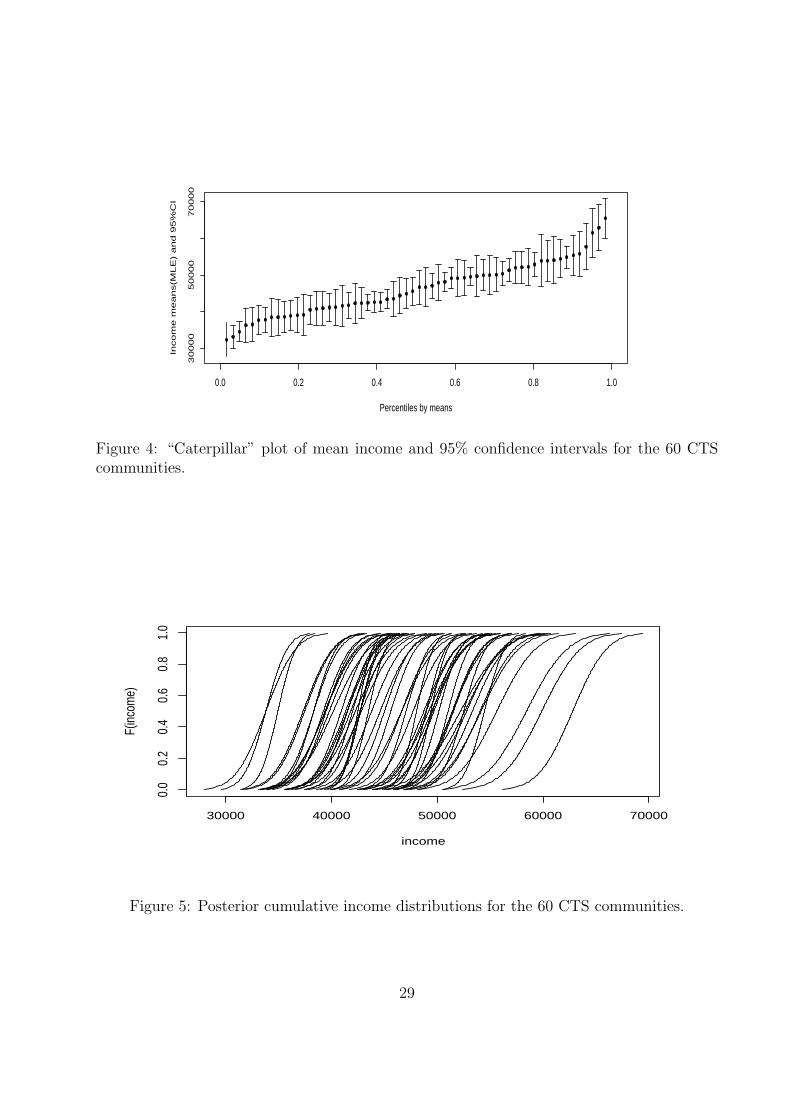
Figure 4 displays the community-specific mean incomes and 95% confidence intervals, ordered

by the community means. (Incomes greater than $150,000 were set aside before computing

community-specific means). There is considerable variation in mean income and the σ2k vary

substantially.

The Gaussian distribution provides a good approximation to the sampling distribution of

community-specific average income. We assume that the true community-specific mean

incomes are also Gaussian, a less tenable assumption, but sufficiently accurate for our illus-

trative purpose. We used the marginal likelihood to estimate the prior mean (µ = $46, 118)

and standard deviation (τ = $6834) and conduct a plug-in (naive) empirical Bayes analysis.

We calculate estimates based on posterior distributions from the plug-in prior.

When the posterior distributions are stochastically ordered, all three estimators are identical.

16

Figure 5 shows that though the posterior cdfs do cross, they are “almost” stochastically

ordered.

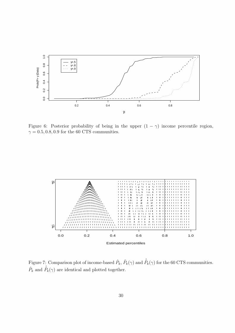
Figure 6 shows predictive performance and is similar to Figure 3. The data set is reasonably

informative, but as is usually the case, the predictive value for the (above γ)/(below γ)

classification is only moderate. For example, the posterior probability is only about 0.50 that

a community with estimated percentile = 0.8 truly is in the upper 20% of the percentiles

and the estimated percentile must exceed 0.9 before this probability is greater than 0.8.

Figure 7 displays percentiles comparing the three estimators (for the CTS income data, Pk ≡ˆPk(γ) and so only two estimators are displayed). All three sets of percentiles produce the

same categorization above and below the γ = 0.8 cut point (none of the lines cross the γ = 0.8

vertical line). Interestingly, because πk(0.8) = 0 for 26 of the communities, Pk(γ) produces

identical percentiles for them relative to the γ = 0.8 cut point. The ˆPk(γ) percentiles break

these ties by optimizing SEL subject to maintaining the (above γ)/(below γ) categorization.

The pattern of ties changes with γ. For example, when γ = 0.5, only 6 of the original 26 are

tied, but now 5 other communities are tied at the largest Pk(γ) with πk(0.5) = 1.

The ties result from our calculating the posterior probabilities via a finite (n = 4000) Monte

Carlo sample from the posterior distribution. As n → ∞, the estimated posterior for each

community would indicate a non-zero chance to be in each (above γ)/(below γ) region.

However, the differences in actual probabilities are so small that it is appropriate to treat

them as tied.

8 Discussion

Table 1 clearly shows that percentiles based on the Y s or on the posterior means of the

target parameter can perform well in general but should not be used to rank or percentile.

Effective approaches must be invariant with respect to a monotone transform of the target

parameter(e.g., the θs). Basing inferences on the representation (2) ensures this invariance.

The Pk that optimize L (SEL) are “general purpose” with no explicit attention to optimizing

17

the (above γ)/(below γ) classification. When posterior distributions are not stochastically

ordered (i.e., when choice of loss function matters), our simulations show that though L0/1(γ),

Pk(γ) and ˆPk(γ) are optimal for their respective loss functions and outperform Pk, Pk per-

forms well for a broad range of γ values. In some scenarios the benefits of using alternatives

to it are notable and in other cases quite small, so the decision to replace Pk by other

candidates must depend on the trade-off between the benefits of reporting general purpose

percentiles and specific targeting of a loss function other than L.

For L, P is optimal, Pk(γ) can perform poorly, especially for extreme γ and gmv 6= 1 ; ˆPk(γ)

is almost identical to Pk. For L(γ), Pk(γ) is optimal, P and ˆPk(γ) perform reasonably well.

For L‡(γ), Pk(γ) is best, Pk performs reasonably well; ˆPk(γ) is worst, but not very far from

the optimal. Recall that ˆPk(γ) will be optimal for Lw0/1 with a suitably small w and should

perform well for a broad range of w values. Though by no means optimal, ˆPk(γ) performs

very well for ÃL‡.

Importantly, as do Liu et al. (2004) and Lockwood et al. (2002), we show that even the

optimal estimates can perform poorly, unless the data are highly informative (gmv is small).

Therefore, assessments such as those in Figures 3 and 6 should be part of any analysis.

Though the estimation approach applies to general models, we have only studied perfor-

mance for the fully parametric, Gaussian/Gaussian model with a known prior distribution.

Results will be essentially identical for empirical Bayes (or Bayes empirical Bayes) for K suffi-

ciently large. Additional studies for a two component Gaussian mixture prior, a “frequentist

scenario” with a fixed set of parameters and repeated sampling only from the Gaussian

sampling distribution conditional on these parameters, and a robust Bayes analysis based on

flexible priors such as the Dirichlet Process (Escobar 1994) will address efficiency and robust-

ness. Broadening performance evaluations to other sampling distributions (e.g., Poisson) is

important.

The new loss functions we consider address classification into the (above γ)/(below γ) cate-

gories. Extensions to three categories (below γ1, between γ1 and γ2; above γ2) will address

the goal of identifying the top, middle and bottom performers. Characterizing and comput-

18

ing the optimizers for these loss functions is challenging, though we predict that, as for the

(above γ)/(below γ) context we have studied, Pk will perform well.

A AppendixA.1 Optimizing weighted squared error loss (WSEL)

Theorem 5. Under weighted squared error loss:

∑

k

ωk

(Rest

k −Rk

)2, (13)

the optimal rank estimates are

Rk = E(Rk|Y) =∑

j

Pj,k(Y) =∑

j

pr(θk ≥ θj|Y).

Proof. (We drop conditioning on Y)

E∑

k

ωk

(Rest

k −Rk

)2=

∑

k

ωkE(Rest

k −Rk + Rk −Rk

)2

=∑

k

ωkE[(Rest

k −Rk)2 + (Rk −Rk)

2]

≥∑

k

ωkE(Rk −Rk)2

Thus, the Rk are optimal.

When all wk ≡ w,

Rk = rank of (Rk)

optimizes (13) subject to the Rk exhausting the integers (1, . . . , K). To see this, if 0 ≤E(Ri) = mi ≤ E(Rj) = mj, ri < rj, then

E(Ri − ri)2 + E(Rj − rj)

2 = Var(Ri) + Var(Rj) + (mi − ri)2 + (mj − rj)

2

< Var(Ri) + Var(Rj) + (mi − rj)2 + (mj − ri)

2

= E(Ri − rj)2 + E(Rj − ri)

2

and the Rk are optimal.

19

For general wk there is no closed form solution, but the following sorting-based algorithm

(letting ωji =ωj

ωi) based on:

(mi − ri)2 + ωji(mj − rj)

2 < (mi − rj)2 + ωji(mj − ri)

2, if rj > ri

⇐⇒ (rj − ri)((1− ωji)(ri + rj − 2mj) + 2(mj −mi)) > 0, if rj > ri

⇐⇒ (1− ωji)(ri + rj − 2mj) + 2(mj −mi) > 0, if rj > ri. (14)

will help to solve the problem.

Theorem 6. Starting from any initial ranks, iteratively switch the position of unit i and unit

j, i, j = 1, ...K, if inequality (14) is satisfied will lead to optimal ranking under the weighted

square loss function (13).

Proof. Since each switch will decrease the expected loss and there are at most n! possible

values of the expected loss , the switches will stop at some step. When this iteration stops, for

any i, j, inequality (14) will not be satisfied. On the other hand, the optimal ranking result

exist due to the fact that there are at most n! possible ranking results, and a necessary

condition of the optimality is that no pair of coordinates i, j will satisfy inequality (14).

This means that the optimal ranking result has the exact same order as the ranking result

at stop.

However, the convergence can be very slow. After unit i and unit j are compared and

ordered, if unit i is compared to some other unit k and switch happens, then i should be

compared to j again. This conclusion tell us that pairwise switch sorting based optimization

algorithm is impractical in our case.

A.2 Proof of Theorem 2

Lemma 1. If a1 + a2 ≥ 0 and b1 ≤ b2, then

a1b1 + a2(1− b2) ≤ a1b2 + a2(1− b1).

20

Proof.

a1b1 + a2(1− b2) ≤ a1b2 + a2(1− b1) ⇔ a1b1 − a2b2 ≤ a1b2 − a2b1

⇔ (a1 + a2)b1 ≤ (a1 + a2)b2.

Lemma 2. (Rearrangement Inequality,see Hardy et al. (1967)) If a1 ≤ a2 ≤ ... ≤ an and

b1 ≤ b2 ≤ ... ≤ bn, b(1), b(2), ...b(n) is a permutation of b1, b2, ...bn, thenn∑

i=1

aibn+1−i ≤n∑

i=1

aib(i) ≤n∑

i=1

aibi.

Proof. For n = 2 we use the ranking inequality:

a1b2 + a2b1 ≤ a1b1 + a2b2 ⇔ (a2 − a1)(b2 − b1) ≥ 0.

For n > 2, there exists a minimum and a maximum in all n! combinations of sums of

products. By the result for n = 2, the necessary condition for the sum to reach the minimum

is that any pair of indices (i1, i2), (ai1, ai2) and (bi1, bi2) must have the inverse order; to reach

the maximum, they must have same order. Therefore, except in the trivial cases where there

are ties inside {ai} or {bi},∑n

i=1 aibn+1−i is the only candidate to reach the minimum and∑n

i=1 aibi is the only candidate to reach the maximum.

Continuing the proof, let

Φ = {Rest = (Rest1 , ...Rest

K ) : any permutation of 1 to K }

and denote by

{j1, j2, ...jK} =argminRest ∈ Φ

E(LRestK

(γ, p, q, c))

the optimum ranking. Let R(i) = Rk if jk = i (i.e., i is the optimum rank of the kth unit).

Then,

E(LRestK

(γ, p, q, c)) =

[γ(K+1)]∑i=1

|γ(K + 1)− i|ppr(R(i) ≥ γ(K + 1))

+K∑

i=[γ(K+1)]+1

c|i− γ(K + 1)|q(1− pr(R(i) ≥ γ(K + 1))).

For optimum ranking, the following conditions are necessary.

21

1. By Lemma 1, for any (i1, i2) satisfying (1 ≤ i1 ≤ [γ(K +1)], [γ(K + 1)] + 1 ≤ i2 ≤ K),

it is required that pr(R(i1) ≥ γ(K + 1)) ≤ pr(R(i2) ≥ γ(K + 1)). To satisfy this

condition, divide the units into two groups by picking the largest K − [γ(K + 1)] from

{pr(Rk ≥ γ(K + 1)) : k = 1, ...K} to be the largest (1− γ)K ranks.

2. By Lemma 2

(a) For the set {k : Rk = R(i), i = 1, · · · , [γ(K + 1)]}, since |γ(K + 1) − i|p is a

decreasing function of i, we require that pr(R(i1) ≥ γ(K + 1)) ≥ pr(R(i2) ≥γ(K + 1)) if i1 > i2. Therefore, for the units with ranks (1, . . . γK), the ranks

should be determined by ranking the pr(Rk ≥ γ(K + 1)).

(b) For the set {k : Rk = R(i), i = [γ(K + 1)] + 1, · · · , K}, since |i − γ(K + 1)|q is

an increasing function of i, we require that pr(R(i1) ≥ γ(K + 1)) ≥ pr(R(i2) ≥γ(K + 1)) if i1 > i2. Therefore, for the units with ranks (γK + 1, . . . , K), the

ranks should be determined by ranking the pr(Rk ≥ γ(K + 1)).

These conditions imply that the Rk(γ) (Pk(γ)) are optimal. By the proof of Lemma 2, we

know that the optimization is not unique when there are ties in pr(Rk ≥ γ(K + 1)).

A.3 Optimization procedure for L†

Similar to the proof of Theorem 2, we begin with a necessary condition for optimization.

Denote by R(i1), R(i2) the rank random variables for coordinates whose ranks are estimated

as i1, i2, where i1 < γ(K + 1), i2 > γ(K + 1). Let

pr(R(i1) ≥ γ(K + 1)) = p1, pr(R(i2) ≥ γ(K + 1)) = p2.

For the index selection to be optimal,

E[(R(i1) − γ(K + 1))2|R(i1) ≥ γ(K + 1)]p1 + cE[(R(i2) − γ(K + 1))2|R(i2) < γ(K + 1)](1− p2)

≤ cE[(R(i1) − γ(K + 1))2|R(i1) < γ(K + 1)](1− p1) + E[(R(i2) − γ(K + 1))2|R(i2) ≥ γ(K + 1)]p2.

The following is equivalent to the foregoing.

E[(R(i1) − γ(K + 1))2|R(i1) ≥ γ(K + 1)]p1 − cE[(R(i1) − γ(K + 1))2|R(i1) < γ(K + 1)](1− p1)

≤ E[(R(i2) − γ(K + 1))2|R(i2) ≥ γ(K + 1)]p2 − cE[(R(i2) − γ(K + 1))2|R(i2) < γ(K + 1)](1− p2).

22

Therefore, with pk = pr(Rk ≥ γ(K + 1)) the optimal ranks split the θs into a lower fraction

and an upper fraction by ranking the quantity,

E[(Rk − γ(K + 1))2|Rk ≥ γ(K + 1)]pk − cE[(Rk − γ(K + 1))2|Rk < γ(K + 1)](1− pk).

This result is useful and different from that of WSEL in section A.1 in the sense that we can

now successfully get a quantity depend on unit index i only. However, as for L0/1 optimizing

of L† does not induce an optimal ordering in the two groups. A second stage loss, for example

SEL, can be imposed within the two groups.

A.4 Optimizing L‡

Similar to that of WSEL in section A.1, pairwise switch algorithm is impractical because

quantity for comparison depends on the position and thus in each iteration, all pairwise rela-

tion have to been check again. We have not identified a general representation or algorithm

for the optimal ranks. However, we have developed the following relation between L†, L and

L‡. Note that when either ABk(γ, Pk, Pestk ) 6= 0 or BAk(γ, Pk, P

estk ) 6= 0 it must be the case

that either P estk ≥ γ ≥ Pk or Pk ≥ γ ≥ P est

k . Equivalently,

|Pk − P estk | = |Pk − γ|+ |P est

k − γ|.

Now, suppose c > 0, p ≥ 1, q ≥ 1 and let m = max(p, q). Then, using the inequality

21−m ≤ am + (1− a)m ≤ 1 for 0 ≤ a ≤ 1, we have that (L + L†) ≤ L‡ ≤ 2m−1(L + L†).

Specifically, if p = q = 1, L‡ = L + L†; if p = q = 2, then (L + L†) ≤ L‡ ≤ 2(L + L†).

Similarly, when c > 0, p ≤ 1, q ≤ 1, (L + L†) ≥ L‡ ≥ 2m−1(L + L†). Therefore, L and L† can

be used to control L‡.

References

Carlin, B. and T. Louis (2000). Bayes and Empirical Bayes Methods for Data Analysis (2nd

ed.). Boca Raton, FL: Chapman and Hall/CRC Press.

Center for Studying Health System Change (2003). Community Tracking Study Household

Survey, 2000-2001: ICPSR version. Ann Arbor, MI: Inter-university Consortium for

Political and Social Research.

23

Christiansen, C. and C. Morris (1997). Improving the statistical approach to health care

provider profiling. Annals of Internal Medicine 127, 764–768.

Conlon, E. and T. Louis (1999). Addressing multiple goals in evaluating region-specific risk

using Bayesian methods. In A. Lawson, A. Biggeri, D. Bohning, E. Lesaffre, J.-F. Viel, and

R. Bertollini (Eds.), Disease Mapping and Risk Assessment for Public Health, Chapter 3,

pp. 31–47. Wiley.

Devine, O. and T. Louis (1994). A constrained empirical Bayes estimator for incidence rates

in areas with small populations. Statistics in Medicine 13, 1119–1133.

Devine, O., T. Louis, and M. Halloran (1994). Empirical Bayes estimators for spatially

correlated incidence rates. Environmetrics 5, 381–398.

DuMouchel, W. (1999). Bayesian data mining in large frequency tables, with an application

to the FDA spontaneous reporting system (with discussion). The American Statistician 53,

177–190.

Escobar, M. (1994). Estimating normal means with a Dirichlet process prior. Journal of the

American Statistical Association 89, 268–277.

Gelman, A. and P. Price (1999). All maps of parameter estimates are misleading. Statistics

in Medicine 18, 3221–3234.

Goldstein, H. and D. Spiegelhalter (1996). League tables and their limitations: statistical

issues in comparisons of institutional performance (with discussion). Journal of the Royal

Statistical Society Series A 159, 385–443.

Hardy, G. H., J. E. Littlewood, and G. Polya (1967). Inequalitites (2nd ed.). Cambridge

University Press.

Kemper, P., D. Blumenthal, J. M. Corrigan, P. J. Cunningham, S. M. Felt, J. M. Grossman,

L. Kohn, C. E. Metcalf, R. F. St. Peter, R. C. Strouse, and P. B. Ginsburg (1996, Summer).

The design of the community tracking study: A longitudinal study of health system change

and its effects on people. INQUIRY 33, 195–206.

24

Laird, N. M. and T. A. Louis (1989). Empirical Bayes ranking methods. Journal of Educa-

tional Statistics 14, 29–46.

Landrum, M., S. Bronskill, and S.-L. Normand (2000). Analytic methods for constructing

cross-sectional profiles of health care providers. Health Services and Outcomes Research

Methodology 1, 23–48.

Liu, J., T. Louis, W. Pan, J. Ma, and A. Collins (2004). Methods for estimating and

interpreting provider-specific, standardized mortality ratios. Health Services and Outcomes

Research Methodology 4, 135–149.

Lockwood, J., T. Louis, and D. McCaffrey (2002). Uncertainty in rank estimation: Im-

plications for value-added modeling accountability systems. Journal of Educational and

Behavioral Statistics 27 (3), 255–270.

Louis, T. and W. Shen (1999). Innovations in Bayes and empirical Bayes methods: Estimat-

ing parameters, populations and ranks. Statistics in Medicine 18, 2493–2505.

McClellan, M. and D. Staiger (1999). The quality of health care providers. Technical Report

7327, National Bureau of Economic Research, Working Paper.

Normand, S.-L. T., M. E. Glickman, and C. A. Gatsonis (1997). Statistical methods for

profiling providers of medical care: Issues and applications. Journal of the American

Statistical Association 92, 803–814.

Shen, W. and T. Louis (1998). Triple-goal estimates in two-stage, hierarchical models.

Journal of the Royal Statistical Society, Series B 60, 455–471.

25

gmv=0.33 gmv=1 gmv=3

200

300

400

500

600

700

800

900

Gaussian−Gaussian Model,rls=1

L

gmv=0.33 gmv=1 gmv=3

100

200

300

400

Gaussian−Gaussian Model,rls=1

L++

Figure 1: Unit-specific, L and L‡ performance as a function of gmv for K = 200, γ = 0.8and rls = 1. The box plots summarize the sampling distribution of unit-specific risk.

26

−1 0 1 2 3

400

500

600

700

800

900

1000

gmv=3,rls=100,γ=0.8log σ2

L

PP(γ)P(γ)

−1 0 1 2 310

020

030

040

0

gmv=3,rls=100,γ=0.8log σ2

L++

PP(γ)P(γ)

−2 −1 0 1 2

0.10

0.15

0.20

gmv=1,rls=100,γ=0.8log σ2

L 0/1

PP(γ)P(γ)

−1 0 1 2 3

0.14

0.16

0.18

0.20

0.22

0.24

0.26

gmv=3,rls=100,γ=0.8log σ2

L 0/1

PP(γ)P(γ)

Figure 2: Loess smoothed, unit-specific L, L‡, and L0/1 performance for Pk, Pk(γ) and ˆPk(γ)as a function of unit-specific variance (σ2

k) for γ = 0.8, rls = 100 and gmv = 1 and 3.

27

0.0 0.2 0.4 0.6 0.8 1.0

0.0

0.2

0.4

0.6

0.8

1.0

P(0.6)

Pr(

p>=

0.6)

gmv=0.33gmv=1gmv=3

gmv=10gmv=100

0.0 0.2 0.4 0.6 0.8 1.0

0.0

0.2

0.4

0.6

0.8

1.0

P(0.8)

Pr(

p>=

0.8)

gmv=0.33gmv=1gmv=3

gmv=10gmv=100

0.0 0.2 0.4 0.6 0.8 1.0

0.0

0.2

0.4

0.6

0.8

1.0

P(0.9)

Pr(

p>=

0.9)

gmv=0.33gmv=1gmv=3

gmv=10gmv=100

Figure 3: Average posterior classification probabilities as a function of the optimally esti-mated percentiles for rls = 1, gmv = (0.33, 1, 3, 10, 100), γ = (0.6, 0.8, 0.9).

28

0.0 0.2 0.4 0.6 0.8 1.0

30

000

50000

70000

Percentiles by means

Incom

e m

ea

ns(M

LE

) an

d 9

5%

CI

Figure 4: “Caterpillar” plot of mean income and 95% confidence intervals for the 60 CTScommunities.

30000 40000 50000 60000 70000

0.0

0.2

0.4

0.6

0.8

1.0

income

F(in

com

e)

Figure 5: Posterior cumulative income distributions for the 60 CTS communities.

29

0.2 0.4 0.6 0.8

0.0

0.2

0.4

0.6

0.8

1.0

P

Pro

b(P

> γ

|Dat

a)

γ=.5γ=.8γ=.9

Figure 6: Posterior probability of being in the upper (1 − γ) income percentile region,γ = 0.5, 0.8, 0.9 for the 60 CTS communities.

0.0 0.2 0.4 0.6 0.8 1.0

Estimated percentiles

P

P

Figure 7: Comparison plot of income-based Pk, Pk(γ) and ˆPk(γ) for the 60 CTS communities.

Pk and ˆPk(γ) are identical and plotted together.

30