Loopy Belief Propagation in the Presence of …vgogate/papers/aistats14-2.pdf · Loopy Belief...
9
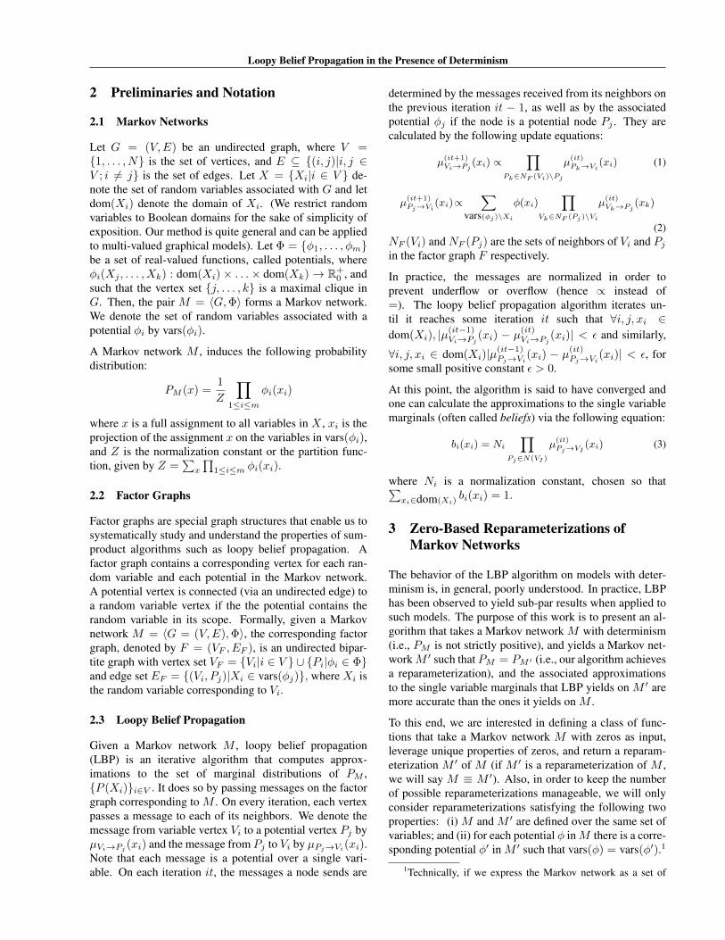
Loopy Belief Propagation in the Presence of Determinism David Smith Vibhav Gogate The University of Texas at Dallas Richardson, TX, 75080, USA [email protected] The University of Texas at Dallas Richardson, TX, 75080, USA [email protected] Abstract It is well known that loopy Belief propagation (LBP) performs poorly on probabilistic graphi- cal models (PGMs) with determinism. In this pa- per, we propose a new method for remedying this problem. The key idea in our method is finding a reparameterization of the graphical model such that LBP, when run on the reparameterization, is likely to have better convergence properties than LBP on the original graphical model. We pro- pose several schemes for finding such reparam- eterizations, all of which leverage unique prop- erties of zeros as well as research on LBP con- vergence done over the last decade. Our exper- imental evaluation on a variety of PGMs clearly demonstrates the promise of our method – it of- ten yields accuracy and convergence time im- provements of an order of magnitude or more over LBP. 1 Introduction Loopy Belief Propagation [15, 16] is a widely used algo- rithm for performing approximate inference in graphical models. The algorithm is exact on tree graphical models and often yields reasonably good poly-time approximations on graphical models having cycles. Its applicability has been demonstrated across a wide variety of fields, includ- ing error correcting codes [6, 12], computer vision [5], and combinatorial optimization [22]. Despite its popularity, LBP is known to display erratic be- havior in practice. In particular, it is still not well under- stood when LBP will yield good approximations. Consid- erable progress has been made towards characterizing the approximations that LBP yields (as fixed points of approx- imate free energy), formalizing sufficient conditions for Appearing in Proceedings of the 17 th International Conference on Artificial Intelligence and Statistics (AISTATS) 2014, Reykjavik, Iceland. JMLR: W&CP volume 33. Copyright 2014 by the au- thors. (i) ensuring the existence of fixed points [23]; (ii) ensuring LBP convergence [21]; and (iii) ensuring the uniqueness of the fixed point to which LBP converges to [8, 9, 14, 17]; and so on. Unfortunately, in practice, even the best bounds are too narrow to be used as an accurate predictor of con- vergence across the spectrum of graphical models. The situation becomes even murkier when LBP is applied to problems that contain determinism. Many of the con- vergence results apply only to problems that model strictly positive distributions. Some work has been done on in- vestigating the effect of determinism on the LBP family of algorithms [4], and some convergence results account for determinism in a restricted manner [14], but in general the existing literature avoids consideration of determinism be- cause of the complications it engenders. The goal of this work is to harness the presence of deter- minism in a PGM in order to help LBP converge more quickly and to more accurate results. In particular, we leverage the following unique property of graphical models (Markov networks) having zeros: if we can derive that the marginal probability of an entry in a potential is zero from other potentials in the Markov network, then we can change that entry to any non-negative real value without changing the underlying distribution. The key idea in this paper is to change such potential entries, namely re-parameterize the Markov network, in such a way that the LBP algorithm converges faster on the new parameterization than on the original Markov network. To achieve this objective, we present two algorithms. The first algorithm leverages techniques from the Satisfiability (SAT) literature to identify a set of potential entries whose values can be altered without affecting the underlying dis- tribution. The second algorithm uses a variety of heuristics to calculate a new set of values in order to create a repa- rameterization of the distribution in which the interactions between neighboring potentials are indicative of models on which LBP tends to be successful. We show experimen- tally that our new approach often allows LBP to converge in fewer iterations and to more accurate results.
Transcript of Loopy Belief Propagation in the Presence of …vgogate/papers/aistats14-2.pdf · Loopy Belief...

Loopy Belief Propagation in the Presence of Determinism
David Smith Vibhav GogateThe University of Texas at Dallas
Richardson, TX, 75080, [email protected]
The University of Texas at DallasRichardson, TX, 75080, USA
Abstract
It is well known that loopy Belief propagation(LBP) performs poorly on probabilistic graphi-cal models (PGMs) with determinism. In this pa-per, we propose a new method for remedying thisproblem. The key idea in our method is findinga reparameterization of the graphical model suchthat LBP, when run on the reparameterization, islikely to have better convergence properties thanLBP on the original graphical model. We pro-pose several schemes for finding such reparam-eterizations, all of which leverage unique prop-erties of zeros as well as research on LBP con-vergence done over the last decade. Our exper-imental evaluation on a variety of PGMs clearlydemonstrates the promise of our method – it of-ten yields accuracy and convergence time im-provements of an order of magnitude or moreover LBP.
1 Introduction
Loopy Belief Propagation [15, 16] is a widely used algo-rithm for performing approximate inference in graphicalmodels. The algorithm is exact on tree graphical modelsand often yields reasonably good poly-time approximationson graphical models having cycles. Its applicability hasbeen demonstrated across a wide variety of fields, includ-ing error correcting codes [6, 12], computer vision [5], andcombinatorial optimization [22].
Despite its popularity, LBP is known to display erratic be-havior in practice. In particular, it is still not well under-stood when LBP will yield good approximations. Consid-erable progress has been made towards characterizing theapproximations that LBP yields (as fixed points of approx-imate free energy), formalizing sufficient conditions for
Appearing in Proceedings of the 17th International Conference onArtificial Intelligence and Statistics (AISTATS) 2014, Reykjavik,Iceland. JMLR: W&CP volume 33. Copyright 2014 by the au-thors.
(i) ensuring the existence of fixed points [23]; (ii) ensuringLBP convergence [21]; and (iii) ensuring the uniqueness ofthe fixed point to which LBP converges to [8, 9, 14, 17];and so on. Unfortunately, in practice, even the best boundsare too narrow to be used as an accurate predictor of con-vergence across the spectrum of graphical models.
The situation becomes even murkier when LBP is appliedto problems that contain determinism. Many of the con-vergence results apply only to problems that model strictlypositive distributions. Some work has been done on in-vestigating the effect of determinism on the LBP family ofalgorithms [4], and some convergence results account fordeterminism in a restricted manner [14], but in general theexisting literature avoids consideration of determinism be-cause of the complications it engenders.
The goal of this work is to harness the presence of deter-minism in a PGM in order to help LBP converge morequickly and to more accurate results. In particular, weleverage the following unique property of graphical models(Markov networks) having zeros: if we can derive that themarginal probability of an entry in a potential is zero fromother potentials in the Markov network, then we can changethat entry to any non-negative real value without changingthe underlying distribution. The key idea in this paper isto change such potential entries, namely re-parameterizethe Markov network, in such a way that the LBP algorithmconverges faster on the new parameterization than on theoriginal Markov network.
To achieve this objective, we present two algorithms. Thefirst algorithm leverages techniques from the Satisfiability(SAT) literature to identify a set of potential entries whosevalues can be altered without affecting the underlying dis-tribution. The second algorithm uses a variety of heuristicsto calculate a new set of values in order to create a repa-rameterization of the distribution in which the interactionsbetween neighboring potentials are indicative of models onwhich LBP tends to be successful. We show experimen-tally that our new approach often allows LBP to convergein fewer iterations and to more accurate results.
Loopy Belief Propagation in the Presence of Determinism
2 Preliminaries and Notation
2.1 Markov Networks
Let G = (V,E) be an undirected graph, where V ={1, . . . , N} is the set of vertices, and E ⊆ {(i, j)|i, j ∈V ; i 6= j} is the set of edges. Let X = {Xi|i ∈ V } de-note the set of random variables associated with G and letdom(Xi) denote the domain of Xi. (We restrict randomvariables to Boolean domains for the sake of simplicity ofexposition. Our method is quite general and can be appliedto multi-valued graphical models). Let Φ = {φ1, . . . , φm}be a set of real-valued functions, called potentials, whereφi(Xj , . . . , Xk) : dom(Xi)× . . .× dom(Xk)→ R+
0 , andsuch that the vertex set {j, . . . , k} is a maximal clique inG. Then, the pair M = 〈G,Φ〉 forms a Markov network.We denote the set of random variables associated with apotential φi by vars(φi).
A Markov network M , induces the following probabilitydistribution:
PM (x) =1
Z
∏1≤i≤m
φi(xi)
where x is a full assignment to all variables in X , xi is theprojection of the assignment x on the variables in vars(φi),and Z is the normalization constant or the partition func-tion, given by Z =
∑x
∏1≤i≤m φi(xi).
2.2 Factor Graphs
Factor graphs are special graph structures that enable us tosystematically study and understand the properties of sum-product algorithms such as loopy belief propagation. Afactor graph contains a corresponding vertex for each ran-dom variable and each potential in the Markov network.A potential vertex is connected (via an undirected edge) toa random variable vertex if the the potential contains therandom variable in its scope. Formally, given a Markovnetwork M = 〈G = (V,E),Φ〉, the corresponding factorgraph, denoted by F = (VF , EF ), is an undirected bipar-tite graph with vertex set VF = {Vi|i ∈ V } ∪ {Pi|φi ∈ Φ}and edge set EF = {(Vi, Pj)|Xi ∈ vars(φj)}, where Xi isthe random variable corresponding to Vi.
2.3 Loopy Belief Propagation
Given a Markov network M , loopy belief propagation(LBP) is an iterative algorithm that computes approx-imations to the set of marginal distributions of PM ,{P (Xi)}i∈V . It does so by passing messages on the factorgraph corresponding to M . On every iteration, each vertexpasses a message to each of its neighbors. We denote themessage from variable vertex Vi to a potential vertex Pj byµVi→Pj
(xi) and the message from Pj to Vi by µPj→Vi(xi).
Note that each message is a potential over a single vari-able. On each iteration it, the messages a node sends are
determined by the messages received from its neighbors onthe previous iteration it − 1, as well as by the associatedpotential φj if the node is a potential node Pj . They arecalculated by the following update equations:
µ(it+1)Vi→Pj
(xi) ∝∏
Pk∈NF (Vi)\Pj
µ(it)Pk→Vi
(xi) (1)
µ(it+1)Pj→Vi
(xi)∝∑
vars(φj)\Xi
φ(xi)∏
Vk∈NF (Pj)\Vi
µ(it)Vk→Pj
(xk)
(2)NF (Vi) and NF (Pj) are the sets of neighbors of Vi and Pjin the factor graph F respectively.
In practice, the messages are normalized in order toprevent underflow or overflow (hence ∝ instead of=). The loopy belief propagation algorithm iterates un-til it reaches some iteration it such that ∀i, j, xi ∈dom(Xi), |µ(it−1)
Vi→Pj(xi) − µ(it)
Vi→Pj(xi)| < ε and similarly,
∀i, j, xi ∈ dom(Xi)|µ(it−1)Pj→Vi
(xi) − µ(it)Pj→Vi
(xi)| < ε, forsome small positive constant ε > 0.
At this point, the algorithm is said to have converged andone can calculate the approximations to the single variablemarginals (often called beliefs) via the following equation:
bi(xi) = Ni∏
Pj∈N(VI )
µ(it)Pj→VI
(xi) (3)
where Ni is a normalization constant, chosen so that∑xi∈dom(Xi)
bi(xi) = 1.
3 Zero-Based Reparameterizations ofMarkov Networks
The behavior of the LBP algorithm on models with deter-minism is, in general, poorly understood. In practice, LBPhas been observed to yield sub-par results when applied tosuch models. The purpose of this work is to present an al-gorithm that takes a Markov network M with determinism(i.e., PM is not strictly positive), and yields a Markov net-workM ′ such that PM = PM ′ (i.e., our algorithm achievesa reparameterization), and the associated approximationsto the single variable marginals that LBP yields on M ′ aremore accurate than the ones it yields on M .
To this end, we are interested in defining a class of func-tions that take a Markov network M with zeros as input,leverage unique properties of zeros, and return a reparam-eterization M ′ of M (if M ′ is a reparameterization of M ,we will say M ≡ M ′). Also, in order to keep the numberof possible reparameterizations manageable, we will onlyconsider reparameterizations satisfying the following twoproperties: (i) M and M ′ are defined over the same set ofvariables; and (ii) for each potential φ inM there is a corre-sponding potential φ′ in M ′ such that vars(φ) = vars(φ′).1
1Technically, if we express the Markov network as a set of
David Smith, Vibhav Gogate
A
B C
(a) A graph
A B C PM
0 0 0 0∗
0 0 1 0∗
0 1 0 00 1 1 1/31 0 0 1/31 0 1 01 1 0 01 1 1 1/3
(b) The joint probabilitydistribution
A B φA,B
0 0 2†
0 1 11 0 11 1 1
A C φA,C
0 0 00 1 11 0 11 1 1
B C φB,C
0 0 10 1 01 0 01 1 1
(c) A set of potentials
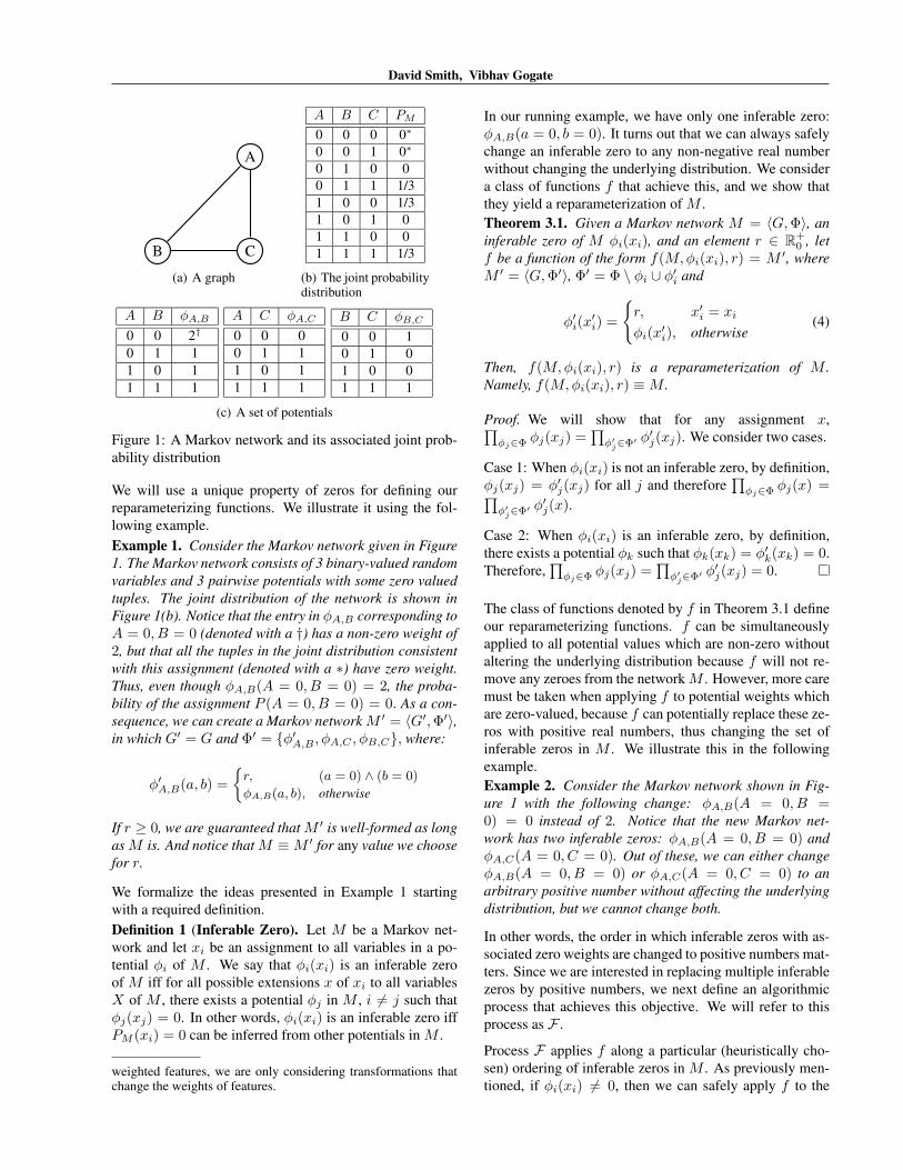
Figure 1: A Markov network and its associated joint prob-ability distribution
We will use a unique property of zeros for defining ourreparameterizing functions. We illustrate it using the fol-lowing example.Example 1. Consider the Markov network given in Figure1. The Markov network consists of 3 binary-valued randomvariables and 3 pairwise potentials with some zero valuedtuples. The joint distribution of the network is shown inFigure 1(b). Notice that the entry in φA,B corresponding toA = 0, B = 0 (denoted with a †) has a non-zero weight of2, but that all the tuples in the joint distribution consistentwith this assignment (denoted with a ∗) have zero weight.Thus, even though φA,B(A = 0, B = 0) = 2, the proba-bility of the assignment P (A = 0, B = 0) = 0. As a con-sequence, we can create a Markov networkM ′ = 〈G′,Φ′〉,in which G′ = G and Φ′ = {φ′A,B , φA,C , φB,C}, where:
φ′A,B(a, b) =
{r, (a = 0) ∧ (b = 0)
φA,B(a, b), otherwise
If r ≥ 0, we are guaranteed that M ′ is well-formed as longas M is. And notice that M ≡M ′ for any value we choosefor r.
We formalize the ideas presented in Example 1 startingwith a required definition.Definition 1 (Inferable Zero). Let M be a Markov net-work and let xi be an assignment to all variables in a po-tential φi of M . We say that φi(xi) is an inferable zeroof M iff for all possible extensions x of xi to all variablesX of M , there exists a potential φj in M , i 6= j such thatφj(xj) = 0. In other words, φi(xi) is an inferable zero iffPM (xi) = 0 can be inferred from other potentials in M .
weighted features, we are only considering transformations thatchange the weights of features.
In our running example, we have only one inferable zero:φA,B(a = 0, b = 0). It turns out that we can always safelychange an inferable zero to any non-negative real numberwithout changing the underlying distribution. We considera class of functions f that achieve this, and we show thatthey yield a reparameterization of M .Theorem 3.1. Given a Markov network M = 〈G,Φ〉, aninferable zero of M φi(xi), and an element r ∈ R+
0 , letf be a function of the form f(M,φi(xi), r) = M ′, whereM ′ = 〈G,Φ′〉, Φ′ = Φ \ φi ∪ φ′i and
φ′i(x′i) =
{r, x′i = xi
φi(x′i), otherwise
(4)
Then, f(M,φi(xi), r) is a reparameterization of M .Namely, f(M,φi(xi), r) ≡M .
Proof. We will show that for any assignment x,∏φj∈Φ φj(xj) =
∏φ′j∈Φ′ φ′j(xj). We consider two cases.
Case 1: When φi(xi) is not an inferable zero, by definition,φj(xj) = φ′j(xj) for all j and therefore
∏φj∈Φ φj(x) =∏
φ′j∈Φ′ φ′j(x).
Case 2: When φi(xi) is an inferable zero, by definition,there exists a potential φk such that φk(xk) = φ′k(xk) = 0.Therefore,
∏φj∈Φ φj(xj) =
∏φ′j∈Φ′ φ′j(xj) = 0.
The class of functions denoted by f in Theorem 3.1 defineour reparameterizing functions. f can be simultaneouslyapplied to all potential values which are non-zero withoutaltering the underlying distribution because f will not re-move any zeroes from the networkM . However, more caremust be taken when applying f to potential weights whichare zero-valued, because f can potentially replace these ze-ros with positive real numbers, thus changing the set ofinferable zeros in M . We illustrate this in the followingexample.Example 2. Consider the Markov network shown in Fig-ure 1 with the following change: φA,B(A = 0, B =0) = 0 instead of 2. Notice that the new Markov net-work has two inferable zeros: φA,B(A = 0, B = 0) andφA,C(A = 0, C = 0). Out of these, we can either changeφA,B(A = 0, B = 0) or φA,C(A = 0, C = 0) to anarbitrary positive number without affecting the underlyingdistribution, but we cannot change both.
In other words, the order in which inferable zeros with as-sociated zero weights are changed to positive numbers mat-ters. Since we are interested in replacing multiple inferablezeros by positive numbers, we next define an algorithmicprocess that achieves this objective. We will refer to thisprocess as F .
Process F applies f along a particular (heuristically cho-sen) ordering of inferable zeros in M . As previously men-tioned, if φi(xi) 6= 0, then we can safely apply f to the

Loopy Belief Propagation in the Presence of Determinism
Algorithm 1 Process F1: Input: A Markov network M2: Output: A Markov Network M ′ such that M ≡M ′, a set Ψ
of configurable parameters of M ′
3: Let Φa = {φi(xi) | φi(xi) is an inferable zero of M}4: Let π(Φa) be an ordering of the elements of Φa5: Ψ = ∅6: M ′ = M7: for i = 1 to |Φa| do8: Let φi(xi) be the i-th entry in π(Φa)9: Let φ′
i(xi) be the potential entry in M ′ corresponding toφi(xi)
10: if φi(xi) 6= 0 then11: M ′ = f(M ′, φ′
i(xi), 1)12: Ψ = Ψ ∪ {φi(xi)}13: else if φ′
i(xi) is an inferable zero of M ′ then14: M ′ = f(M ′, φ′
i(xi), 1)15: Ψ = Ψ ∪ {φi(xi)}16: end if17: end for18: return 〈M ′,Ψ〉
Markov network (Steps 9 and 10). However, if φi(xi) = 0then care must be taken to ensure that xi is also an infer-able zero of the current Markov network M ′ (Steps 12 and13). F sets the value of each inferable zero to 1 (as a place-holder), and it collects the inferable zeros in the set Ψ.
Since the Markov network M ′ at each iteration in F is ei-ther the same or obtained by applying the function f to theMarkov network in the previous iteration, it follows fromTheorem 3.1 thatM ′ is a reparameterization of the Markovnetwork in the previous iteration. Therefore, by using theprinciple of induction, it is straight-forward to show that:
Theorem 3.2. F yields a reparameterization of M .Namely, if F(M) = 〈M ′,Ψ〉, then M ′ ≡M .
Now, notice that each of the potential weights Ψ of M ′
can be set to any element r ∈ R+0 without affecting the
distribution PM . Let ∆(M,Ψ) be any function that assignsany element of R+
0 to each free parameter in Ψ. Then:
Theorem 3.3. ∆(M,Ψ) yields a reparameterization ofM .Namely, if F(M) = 〈M ′,Ψ〉, then ∆(M,Ψ) ≡M .
Thus, we refer to the parameters of Ψ as the free parame-ters of M .
Three practical issues remain with regard to using F forimproving the convergence and accuracy of LBP:
• How to find the inferable zeros of M?• What value of R+
0 should be assigned to each inferredzero in Ψ?• How to choose an ordering for inferable zeros?
We will answer these three questions in the next two sec-tions
4 Finding Inferable Zeros
The computation of f requires inferring some global infor-mation about the given Markov network for every entry ofthe given potential φi. It is well-known that such a task isNP-Hard for arbitrary Markov networks [3]. Fortunately,we do not need to infer the actual probability of each entry;it suffices to know whether or not the probability of eachentry is equal to zero. Even so, such a task is NP-Completefor arbitrary Markov networks. However, with the help ofmodern SAT solving techniques (cf. [20]), even problemswith a large number of variables and clauses can often behandled easily.
It is straightforward to encode the problem of finding thezero-valued marginals of a Markov networkM with binaryrandom variables as a SAT instance. For each random vari-able in M , add a Boolean variable to the SAT instance. Foreach φi(xi) = 0 in M , add the clause ¬ci to the SAT in-stance, where ci is the conjunctive clause corresponding tothe assignment xi.Example 3. Let A, B and C be the Boolean vari-ables associated with three random variables in theMarkov network in Figure 1. Then the conjunctive clausec(A=0,C=0) = (¬A ∧ ¬C), and ¬c(A=0,C=0) = (A ∨ C).
The conjunction of all such clauses forms a SAT instancein conjunctive normal form that is satisfiable iff M iswell-defined (i.e., contains any full assignment x such thatP (x) 6= 0). The problem is only slightly more difficult forMarkov networks with multi-valued random variables (cf.Sang et al. [19]).Example 4. Let A, B and C be the Boolean variables as-sociated with three random variables in the Markov net-work in Figure 1. The SAT instance corresponding to theMarkov network is (A ∨ C) ∧ (B ∨ ¬C) ∧ (¬B ∨ C).
We can use such an encoding in order to determine if anypotential entry is an inferable zero of M . Algorithm 2 de-tails this procedure:
Algorithm 2 Check Inferable Zero1: Input: A Markov network M , an inferable zero candidate,φi(xi)
2: Output: A member of {True, False}3: Let S = ConstructSAT(M )4: Let ci be the conjunctive clause corresponding to xi5: if φi(xi) 6= 0 then6: S = S ∧ ci7: else8: S = (S \ ¬ci) ∧ ci 2
9: end if10: return ¬ isSatisfiable(S)
Example 5. Consider again M from Figure 1. Supposewe want to to determine if φA,B(A = 0, B = 0) is aninferable zero of M . Since φA,B(A = 0, B = 0) = 2 6= 0,we construct the SAT instance as shown in Example 4 andconjoin it with the assignment (¬A)∧(¬B) to yield the SAT

David Smith, Vibhav Gogate
instance S = (A∨C)∧(B∨¬C)∧(¬B∨C)∧(¬A)∧(¬B).S is not satisfiable; hence Algorithm 2 returns True. Thus,φA,B(A = 0, B = 0) is an inferable zero of M .Example 6. Consider the same modification to the Markovnetwork in Figure 1 as detailed in Example 2; namely thatφA,B(A = 0, B = 0) = 0 instead of 2. Again, suppose wewant to to determine if φA,B(A = 0, B = 0) is an inferablezero of M . Since φA,B(A = 0, B = 0) = 0, we constructthe SAT instance S = (A∨B)∧(A∨C)∧(B∨¬C)∧(¬B∨C), remove the clause corresponding to ¬(¬A ∧ ¬B) =(A ∨ B), and add (¬A) ∧ (¬B), yielding a SAT instanceS = (A∨C)∧(B∨¬C)∧(¬B∨C)∧(¬A)∧(¬B). Again,S is not satisfiable; hence Algorithm 2 again returns True.Thus, φA,B(A = 0, B = 0) is an inferable zero of M .
There are a few notes we would like to briefly mention atthis point. First, in the case in which the Markov networkM is pairwise-binary, its corresponding SAT encoding isan instance of 2-SAT. Since each clause added by Algo-rithm 2 contains just a single variable, each inferable zerotest reduces to a 2-SAT satisfiability test, which can be donein linear time using the approach of mapping the problemto one of checking for strongly connected components [1].Second, note that it is not necessary to find all inferred ze-roes in order to apply Algorithm 1. If it is infeasible to ap-ply Algorithm 2 to all φi(xi) ∈ M , one can simply checkonly those potential entries that are troublesome for LBP.We propose a method for heuristically ranking potentialsfor this purpose in Section 5.
5 Setting the Free Parameters of M
Now that we can discover which potential entries can besafely changed without affecting the overall distribution,we must decide how to change them. There are many pos-sible approaches to modifying a Markov network. In thiswork, we have chosen to take advantage of the substantialresearch that establishes sufficient conditions for the con-vergence of LBP to a fixed point [8, 9, 14, 17, 21, 23].
Many of the results on the convergence of LBP rely ondefining some notion of the ‘strength’ of the potential andthen guaranteeing convergence if some relationship amongthese potential strengths holds on the factor graph associ-ated with the given Markov network. These notions areoften defined exclusively on Markov networks that yieldstrictly positive distributions, thus making them unsuitablefor our purposes. However, Mooij and Kappen [14] havedefined a notion of potential strength that is well-definedon many distributions that are not strictly positive, and sowe have chosen to use the formula offered in their work asthe basis for our choice of parameters. We reprint it herefor convenience:
N(φi, j, k) := supα 6=α′
supβ 6=β′
supγ,γ′
2We abuse notation slightly. Take S \ c to mean the SAT in-stance S with the clause c removed.
√φi(αβγ)φi(α′β′γ′)−
√φi(α′βγ)φi(αβ′γ′)√
φi(αβγ)φi(α′β′γ′) +√φi(α′βγ)φi(αβ′γ′)
(5)
Convergence to a unique fixed point, irrespective of initialmessages, is guaranteed if:
maxPj→Vj
∑Pi∈N(Pj)\Pj
∑Vi∈N(Pi)\Vj
N(Pi, i, j) < 1 (6)
Our approach is to develop heuristics that attempt to min-imize this quantity. We present several methods for per-forming this optimization.
Given a Markov network M and some set of free parame-ters Ψ, one has several choices as to how to optimize ele-ments of Ψ for LBP. One can optimize each parameter in-dependently, partition the parameters of Ψ into disjoint setsand optimize each set of parameters independently, or onecan optimize the entire set of parameters in Ψ jointly. Wehave found that optimizing the parameters independentlyyields relatively little gain on the majority of Markov net-works. Conversely, optimizing all the parameters jointlytends to be infeasible on the majority of Markov networks.Hence we have chosen to optimize the free parameters ineach potential jointly.
We present a formal framework for these optimizing func-tions. Define ∆(M,Ψ) = M ′, where M ′ = 〈G,Φ′〉 andΦ′ = {δ(φi, ψi)|φi ∈ Φ, ψi = {φi(xi)|φi(xi) ∈ Ψ}}, andδ(φi, ψi) is any function that takes a potential φ and its freeparameters ψ as input, and returns a new potential φ′ thathas the same scope (vars(φ) = vars(φ′)), but in which allfree parameters have (possibly) different weights.
Thus, ∆(F(M)) = M ′ and M ≡ M ′. That is, a ∆ func-tion takes a Markov network M and a set of free parame-ters in M , and it calls δ on each potential of M along withthe free parameters of that potential, assigns values to allfree parameters, and returns a Markov network M ′ with anequivalent joint distribution.
5.1 The Zero Heuristic- δ0
Perhaps the most obvious heuristic is to simply set all thefree parameters in each potential to 0. The intuitive idea isthat this choice would give LBP the maximum knowledgeabout the global distribution at each potential. In the con-text of Equation 5, such a choice of heuristic turns out to beproblematic, because it forces an evaluation of 1 in morecases. Equation 5 implies that such evaluations will hurtthe performance of LBP, and our experiments corroboratethis hypothesis in many cases, although this heuristic does,in general, help the performance of LBP (see Section 6).
5.2 The Mean Heuristic- δµ
Another computationally inexpensive method is to simplyset all the weights of the free parameters to the mean valueof the weights of the non-free parameters in their respective
Loopy Belief Propagation in the Presence of Determinism
potentials. Clearly, given a graphical model with uniformpseudo-distributions at each potential (and hence an overalldistribution that is uniform), Equation 6 will have a valueof 0, assuring convergence to a unique fixed point. The ideabehind this simple modification is that it brings the pseudo-distribution at each potential closer to the uniform one.
5.3 The Local Min Strength Heuristic- δLMS
This heuristic directly minimizes the quantity in Equation 5via a nonlinear optimization routine. We optimize each po-tential independently. Let x ∈ R+n
0 , where n is the numberof variable values in potential φi. We formulate the opti-mization problem as:
mint∈R+
0 ,x∈R+n0
t subject to gk(x)− t ≤ 0k∈{1,...,m}
where m is equal to the total number of constraints of theform:
gk(x) =
√φi(αβγ)φi(α′β′γ′)−
√φi(α′βγ)φi(αβ′γ′)√
φi(αβγ)φi(α′β′γ′) +√φi(α′βγ)φi(αβ′γ′)
taken over all possible values for α,α′,β,β′, γ, and γ′, suchthat α 6= α′, β 6= β′, and the at least one of the membersof the set {φi(αβγ), φi(α
′β′γ′), φi(α′βγ), φi(αβ′γ′)} is
free parameter and hence equals xi for i ∈ {1, . . . , n}.This formulation is equivalent to minimizing the maximumvalue for gk(x), and hence is equivalent to minimizing thestrength of each potential independently (see Equation 5).
5.4 The Local Min Sum Strength Heuristic- δLMSS
The previous heuristic has the disadvantage that it only at-tempts to minimize the maximum value of the set of con-straints. Even after the minimax is found, we would like tocontinue minimizing the gk(x) for all values of k. One wayto approximate this behavior is to minimize the sum of theconstraints. We formulate the problem as follows:
mint∈R+
0 ,x∈R+n0
t subject to t−m∑k=1
tk ≤ 0
gk(x)− tk ≤ 0k∈{1,...,m}
where the set of constants are the same as those from theprevious heuristic.
5.5 The Local Min Exponential Sum StrengthHeuristic- δLMESS
Although the previous heuristic attempts to minimize overall constraints, it has the disadvantage that it assigns equalpriority to the minimization of all sums, regardless of theirsize. We would like to give larger sums a higher priorityfor minimization. One way to approximate this behavior
is to minimize the exponential sum of the constraints. Weformulate the problem as follows:
mint∈R+
0 ,x∈R+n0
t subject to t−m∑k=1
etk ≤ 0
gk(x)− tk ≤ 0k∈{1,...,m}
where the set of constants are the same as those from theprevious heuristic. Under this formulation, the largest val-ues for gk(x) are assigned weights that decrease exponen-tially faster than the smaller weights, and hence are thepriority for minimization, but after their mins have beenfound, the overall sum can still be minimized by optimiz-ing over the remaining constraints.
5.6 Using the N function as an Ordering Heuristic
The N function can also be used to rank the strength of po-tentials in order to find an ordering for the application of f .Our approach is to order the set of potentials in descend-ing order according to their Nscore. We then apply f toeach entry of each potential along this ordering (we do nosorting of the entries in a given potential).
The choice of this heuristic is motivated by the fact thatthose potentials with higher Nscores are potentially moreproblematic for LBP, and hence adding variable values tothem first is more likely to yield a reparameterization closerto the convergence guarantee.
6 Experiments
The implementation of this algorithm requires a SAT-solverand a nonlinear optimizer. We used Minisat [20] andNLOpt [10] for these tasks, respectively. We experimentedwith the following networks: (1) Ising Models, (2) randomMarkov networks, and (3) random 3-SAT instances. Thepotential values of the randomly generated Ising modelsand Markov networks were set as follows: we draw a ran-dom real number between 0 and 1 from the uniform distri-bution; if the number is smaller than the percent zero valuefor the network, we assign the potential entry a weight of 0;else a real number x is drawn from a Gaussian distributionwith µ = 0 and variance equal to σ, an input parameter.Then we take ex and assign it as the potential value.
6.1 Grid Networks (Ising Models)
To demonstrate the soundness of the concept, we first gen-erated 10 × 10 Ising models with increasing levels of σ ={1, 3, 5}. For each value for σ, we generated networks withdeterminism between 0% to 20% (at 2.5% intervals, 1000graphs at each interval). On each graph we calculated theexact values of the single variable marginals; we then ap-plied a variety of heuristics and ran LBP. Figure 2 shows
David Smith, Vibhav Gogate
�
�
�
�
�
� � �
�
�
��
� �
� �
à
à
àà
à
à
à
à
æ
æ
ææ
æ
æ
æ
æ
ò
ò
ò ò
ò
ò
ò ò
@
@
@
@ @ @ @ @
0.00 0.05 0.10 0.15 0.20
7.6
7.7
7.8
7.9
8.0
%Zeroes
Avg
Nscore
Avg Nscore vs %Zeroes 10x102d1m5mu
� -none � ∆_Μ à ∆_8LMS<
æ ∆_8LMSS< ò ∆_8LMESS< @ ∆_0
�
�
�
�
�
�
�
�
�
�
�
�
� �
�
�
à
à
à
à
à
à
à
à
æ
æ
æ
æ
æ
æ
æ
æ
ò
ò
ò
ò
ò
ò
ò
ò
@
@
@
@
@
@
@
@
0.00 0.05 0.10 0.15 0.20
100
120
140
160
180
%Zeroes
Ite
rati
ons
Avg Iterations vs %Zeroes 10x102d1m5mu
� -none � ∆_Μ à ∆_8LMS<
æ ∆_8LMSS< ò ∆_8LMESS< @ ∆_0
�
�
�
�
�
�
�
�
�
�
�
�
�
�
�
�à
à
à
à
à
à
à
à
æ
æ
æ
æ
æ
ææ
æ
ò
ò
ò
ò
ò
òò
ò
@
@
@
@
@
@
@
@
0.00 0.05 0.10 0.15 0.20
0.0015
0.0020
0.0025
0.0030
0.0035
0.0040
%Zeroes
Hell
inger
Dis
tance
Hellinger Distance vs %Zeroes 10x102d1m5mu
� -none � ∆_Μ à ∆_8LMS<
æ ∆_8LMSS< ò ∆_8LMESS< @ ∆_0
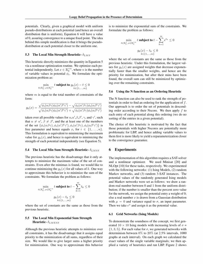
Figure 2: Nscore, iterations to convergence, and Hellinger distance for 10x10 grids of binary variables, generated from anexponential Gaussian distribution with σ = 5.
the results for networks generated with σ = 5. The re-sults indicate a correlation between the Nscore of a graphand many desirable properties under LBP. Networks with alower Nscore converge more often, in fewer iterations, andto more accurate single variable marginals. Thus, even if itis not possible to find an Nscore low enough to guaranteeconvergence for a particular graph, optimizing for its min-imum value will still give a higher chance of obtaining anaccurate approximation.
The heuristics that require optimization outperform thosethat do not by a substantial margin. In general, δLMESS
yields the best results on these types of models and δLMSS
is next best. This result is expected; these two heuristics re-quire the most constraints of any the heuristics tested. Theδ0 heuristic is an anomaly. While it usually creates net-works with poor Nscores, these networks generally yieldsgood approximations, particularly as the value of σ in-creases. This might suggest that our use of 0/0 = 1 in thecalculation of the Nscore is incorrect. However, in manyother varieties of networks, δ0 performs poorly; in manycases, the application of δ0 forces networks that convergeunder standard LBP to never converge.
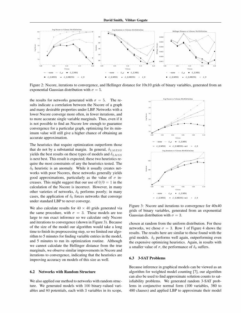
We also calculate results for 40 × 40 grids generated viathe same procedure, with σ = 3. These models are toolarge to run exact inference so we calculate only Nscoreand iterations to convergence (shown in Figure 3). Becauseof the size of the model our algorithm would take a longtime to finish its preprocessing step, so we limited our algo-rithm to 5 minutes for finding variable entries in the model,and 5 minutes to run its optimization routine. Althoughwe cannot calculate the Hellinger distance from the truemarginals, we observe similar improvements in Nscore anditerations to convergence, indicating that the heuristics areimproving accuracy on models of this size as well.
6.2 Networks with Random Structure
We also applied our method to networks with random struc-ture. We generated models with 100 binary-valued vari-ables and 80 potentials, each with 3 variables in its scope,
�
�
�
�
�
�
�
�
�
–
–
–
–
–
–
––
–
ð
ð
ð
ðð ð ð
ðð
2
2
2
22 2 2
22
¢
¢
¢
¢
¢¢ ¢
¢
¢
@
@
@
@
@
@
@
@
@
0.00 0.02 0.04 0.06 0.08 0.10
3.0
3.2
3.4
3.6
3.8
4.0
%Zeroes
Avg
Nsc
ore
Avg Nscore vs %Zeroes 40x402d1m3mu
� -none – ∆_Μ ð ∆_8LMS<
2 ∆_8LMSS< ¢ ∆_8LMESS<-no1 @ ∆_0
�
�
�
�
�
��
� �
–
–
–
–
–
––
–
–
ð
ð
ð
ð
ð
ð
ð
ðð
2
2
2
2
2
22
22
¢
¢
¢
¢
¢
¢
¢
¢ ¢
@
@
@
@
@
@@
@ @
0.00 0.02 0.04 0.06 0.08 0.10
350
400
450
%Zeroes
Itera
tions
Avg Iterations vs %Zeroes 40x402d1m3mu
� -none – ∆_Μ ð ∆_8LMS<
2 ∆_8LMSS< ¢ ∆_8LMESS<-no1 @ ∆_0
Figure 3: Nscore and iterations to convergence for 40x40grids of binary variables, generated from an exponentialGaussian distribution with σ = 3.
chosen at random from the uniform distribution. For thesenetworks, we chose σ = 3. Row 1 of Figure 4 shows theresults. The results here are similar to those found with thegrid models. δ0 performs well again, outperforming eventhe expensive optimizing heuristics. Again, in results witha smaller value of σ, the performance of δ0 suffers.
6.3 3-SAT Problems
Because inference in graphical models can be viewed as analgorithm for weighted model counting [7], our algorithmcan also be used to find approximate solution counts to sat-isfiability problems. We generated random 3-SAT prob-lems in conjunctive normal form (100 variables, 380 to480 clauses) and applied LBP to approximate their model
Loopy Belief Propagation in the Presence of Determinism
�
��
�
�
�� �
�
�� �
�
�
�
��
��
�
�
�
� ��
� �
� � �
�
�
à
àà
à
à
à
à à à
àà
à àà
à
à
æ
æ
ææ
ææ
æ ææ
æ
æ
æ
æ
æ
æ æò
òò
ò
òò
òò
òò
òò
ò
ò
ò ò@
@@
@@
@ @@
@@
@
@@
@
@
@
0.0 0.1 0.2 0.3 0.4
0.4
0.5
0.6
0.7
0.8
0.9
%Zeroes
%C
onverged
%Converged vs %Zeroes 100v80p3s2d1m3mu
� -none � ∆_Μ à ∆_8LMS<
æ ∆_8LMSS< ò ∆_8LMESS< @ ∆_0
�
�
�
�
�� �
� ��
� �
�
�
�
�
�
��
��
� � � �
��
�� �
�
�
à
àà
àà
à à à à
à
àà
àà
à
à
æ
ææ
ææ
æ æ æ ææ
ææ
æ
æ
æ æ
ò
òò
òò ò ò
ò ò ò
ò ò
ò
ò
ò ò
@
@
@
@ @ @ @@
@@
@
@
@
@
@
@
0.0 0.1 0.2 0.3 0.4
100
150
200
%Zeroes
Ite
rati
ons
Avg Iterations vs %Zeroes 100v80p3s2d1m3mu
� -none � ∆_Μ à ∆_8LMS<
æ ∆_8LMSS< ò ∆_8LMESS< @ ∆_0
�� �
��
��
��
�
�� � �
�
�
�� �
��
��
��
�
�
�
�
�
�
�
àà à
àà
àà
à à
à
à
à
à
à
à
à
ææ æ æ
ææ
ææ
ææ
æ æ æ æ
æ
æ
òò
ò òò
òò
ò ò
òò ò
òò
ò
ò
@@ @
@@
@ @@ @
@
@@ @
@@
@
0.0 0.1 0.2 0.3 0.4
0.000
0.005
0.010
0.015
0.020
0.025
0.030
0.035
%Zeroes
Hell
inger
Dis
tance
Hellinger Distance vs %Zeroes 100v80p3s2d1m3mu
� -none � ∆_Μ à ∆_8LMS<
æ ∆_8LMSS< ò ∆_8LMESS< @ ∆_0
�
��
� �
�
� �� �
�
à
à
à
à
à
à
à à à
à
à
òò
ò
ò
ò
ò
òò
ò ò
ò
@
@
@@
@ @@ @
@
@
@
380 400 420 440 460 480
0.0
0.2
0.4
0.6
0.8
1.0
ðClauses
%C
onverged
%Converged vs ðClauses cnf
� -none à ∆_8LMS< ò ∆_8LMESS< @ ∆_0
��
� ��
�
�� � �
�
à
à
à
à
à
à
à à àà
à
ò ò
ò
ò
ò
ò
ò òò
ò
ò
@
@
@
@
@@ @
@ @@
@
380 400 420 440 460 480
0
100
200
300
400
ðClauses
Ite
rati
ons
Avg Iterations vs ðClauses cnf
� -none à ∆_8LMS< ò ∆_8LMESS< @ ∆_0
�
�
�
�
��
�
�
�
�
�à
à
à
à à
à à àà
à à
ò
ò
òò
ò
ò òò ò
ò ò
@
@
@
@
@
@
@@
@
@
@
380 400 420 440 460 480
0.00
0.02
0.04
0.06
0.08
ðClauses
Hell
inger
Dis
tance
Hellinger Distance vs ðClauses cnf
� -none à ∆_8LMS< ò ∆_8LMESS< @ ∆_0
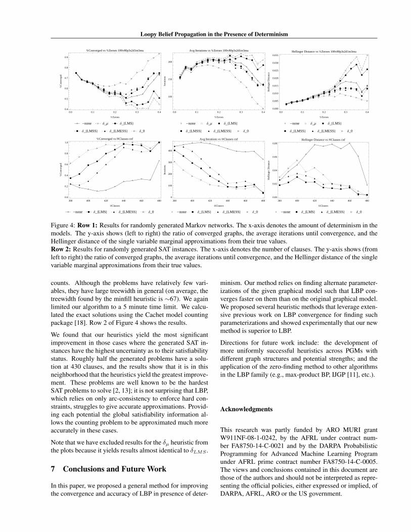
Figure 4: Row 1: Results for randomly generated Markov networks. The x-axis denotes the amount of determinism in themodels. The y-axis shows (left to right) the ratio of converged graphs, the average iterations until convergence, and theHellinger distance of the single variable marginal approximations from their true values.Row 2: Results for randomly generated SAT instances. The x-axis denotes the number of clauses. The y-axis shows (fromleft to right) the ratio of converged graphs, the average iterations until convergence, and the Hellinger distance of the singlevariable marginal approximations from their true values.
counts. Although the problems have relatively few vari-ables, they have large treewidth in general (on average, thetreewidth found by the minfill heuristic is ∼67). We againlimited our algorithm to a 5 minute time limit. We calcu-lated the exact solutions using the Cachet model countingpackage [18]. Row 2 of Figure 4 shows the results.
We found that our heuristics yield the most significantimprovement in those cases where the generated SAT in-stances have the highest uncertainty as to their satisfiabilitystatus. Roughly half the generated problems have a solu-tion at 430 clauses, and the results show that it is in thisneighborhood that the heuristics yield the greatest improve-ment. These problems are well known to be the hardestSAT problems to solve [2, 13]; it is not surprising that LBP,which relies on only arc-consistency to enforce hard con-straints, struggles to give accurate approximations. Provid-ing each potential the global satisfiability information al-lows the counting problem to be approximated much moreaccurately in these cases.
Note that we have excluded results for the δµ heuristic fromthe plots because it yields results almost identical to δLMS .
7 Conclusions and Future Work
In this paper, we proposed a general method for improvingthe convergence and accuracy of LBP in presence of deter-
minism. Our method relies on finding alternate parameter-izations of the given graphical model such that LBP con-verges faster on them than on the original graphical model.We proposed several heuristic methods that leverage exten-sive previous work on LBP convergence for finding suchparameterizations and showed experimentally that our newmethod is superior to LBP.
Directions for future work include: the development ofmore uniformly successful heuristics across PGMs withdifferent graph structures and potential strengths; and theapplication of the zero-finding method to other algorithmsin the LBP family (e.g., max-product BP, IJGP [11], etc.).
Acknowledgments
This research was partly funded by ARO MURI grantW911NF-08-1-0242, by the AFRL under contract num-ber FA8750-14-C-0021 and by the DARPA ProbabilisticProgramming for Advanced Machine Learning Programunder AFRL prime contract number FA8750-14-C-0005.The views and conclusions contained in this document arethose of the authors and should not be interpreted as repre-senting the official policies, either expressed or implied, ofDARPA, AFRL, ARO or the US government.
David Smith, Vibhav Gogate
References[1] Bengt Aspvall, Michael F Plass, and Robert Endre
Tarjan. A linear-time algorithm for testing the truthof certain quantified boolean formulas. InformationProcessing Letters, 14(4):195, 1982.
[2] Peter Cheeseman, Bob Kanefsky, and William M Tay-lor. Where the really hard problems are. In IJCAI,volume 91, pages 331–337, 1991.
[3] G. F. Cooper. The computational complexity of prob-abilistic inference using Bayesian belief networks.Artificial Intelligence, 42(2-3):393–405, March 1990.
[4] Rina Dechter and Robert Mateescu. A simple in-sight into iterative belief propagation’s success. InProceedings of the Nineteenth conference on Uncer-tainty in Artificial Intelligence, pages 175–183. Mor-gan Kaufmann Publishers Inc., 2003.
[5] Pedro F Felzenszwalb and Daniel P Huttenlocher. Ef-ficient belief propagation for early vision. Interna-tional journal of computer vision, 70(1):41–54, 2006.
[6] Marc PC Fossorier, Miodrag Mihaljevic, and HidekiImai. Reduced complexity iterative decoding of low-density parity check codes based on belief prop-agation. Communications, IEEE Transactions on,47(5):673–680, 1999.
[7] V. Gogate and P. Domingos. Formula-based proba-bilistic inference. In Proceedings of the Twenty-SixthConference on Uncertainty in Artificial Intelligence,pages 210–219, 2010.
[8] Tom Heskes. On the uniqueness of loopy be-lief propagation fixed points. Neural Computation,16(11):2379–2413, 2004.
[9] Alexander T Ihler, John W Fisher III, Alan S Willsky,and David Maxwell Chickering. Loopy belief prop-agation: convergence and effects of message errors.Journal of Machine Learning Research, 6(5), 2005.
[10] Steven G Johnson. The nlopt nonlinear-optimizationpackage, 2010.
[11] R. Mateescu, K. Kask, V. Gogate, and R. Dechter. It-erative Join Graph Propagation algorithms. Journal ofArtificial Intelligence Research, 37:279–328, 2010.
[12] Robert J. McEliece, David J. C. MacKay, and Jung-Fu Cheng. Turbo decoding as an instance of pearl’sbelief propagation algorithm. Selected Areas in Com-munications, IEEE Journal on, 16(2):140–152, 1998.
[13] David Mitchell, Bart Selman, and Hector Levesque.Hard and easy distributions of sat problems. In AAAI,volume 92, pages 459–465. Citeseer, 1992.
[14] Joris Mooij and Hilbert Kappen. Sufficient conditionsfor convergence of loopy belief propagation. arXivpreprint arXiv:1207.1405, 2012.
[15] K. P. Murphy, Y. Weiss, and M. I. Jordan. Loopy Be-lief Propagation for Approximate Inference: An Em-pirical Study. In Proceedings of the Fifteenth Confer-ence on Uncertainty in Artificial Intelligence, pages467–475, 1999.
[16] Judea Pearl. Probabilistic reasoning in intelligent sys-tems: networks of plausible inference. Morgan Kauf-mann, 1988.
[17] Tanya Gazelle Roosta, Martin J Wainwright, andShankar S Sastry. Convergence analysis ofreweighted sum-product algorithms. Signal Process-ing, IEEE Transactions on, 56(9):4293–4305, 2008.
[18] Tian Sang, Fahiem Bacchus, Paul Beame, Henry AKautz, and Toniann Pitassi. Combining componentcaching and clause learning for effective model count-ing. SAT, 4:7th, 2004.
[19] Tian Sang, Paul Beame, and Henry Kautz. Solv-ing bayesian networks by weighted model counting.In Proceedings of the Twentieth National Conferenceon Artificial Intelligence (AAAI-05), volume 1, pages475–482, 2005.
[20] Niklas Sorensson and Niklas Een. Minisat v1. 13-a sat solver with conflict-clause minimization. SAT,2005:53, 2005.
[21] Sekhar C Tatikonda and Michael I Jordan. Loopy be-lief propagation and gibbs measures. In Proceedingsof the Eighteenth conference on Uncertainty in artifi-cial intelligence, pages 493–500. Morgan KaufmannPublishers Inc., 2002.
[22] Chen Yanover and Yair Weiss. Finding the ai mostprobable configurations using loopy belief propaga-tion. Advances in Neural Information Processing Sys-tems, 16:289, 2004.
[23] Jonathan S Yedidia, William T Freeman, and YairWeiss. Constructing free-energy approximations andgeneralized belief propagation algorithms. Informa-tion Theory, IEEE Transactions on, 51(7):2282–2312,2005.