Loopy Belief Propagation for Bipartite Maximum...
67
Loopy Belief Propagation for Bipartite Maximum Weight b-Matching Bert Huang and Tony Jebara Computer Science Department Columbia University New York, NY 10027
Transcript of Loopy Belief Propagation for Bipartite Maximum...
Loopy Belief Propagation for Bipartite Maximum Weight
b-Matching
Bert Huang and Tony JebaraComputer Science Department
Columbia UniversityNew York, NY 10027
1. Bipartite Weighted b-Matching
2. Edge Weights As a Distribution
3. Efficient Max-Product
4. Convergence Proof Sketch
5. Experiments
6. Discussion
Outline
1. Bipartite Weighted b-Matching
2. Edge Weights As a Distribution
3. Efficient Max-Product
4. Convergence Proof Sketch
5. Experiments
6. Discussion
Outline
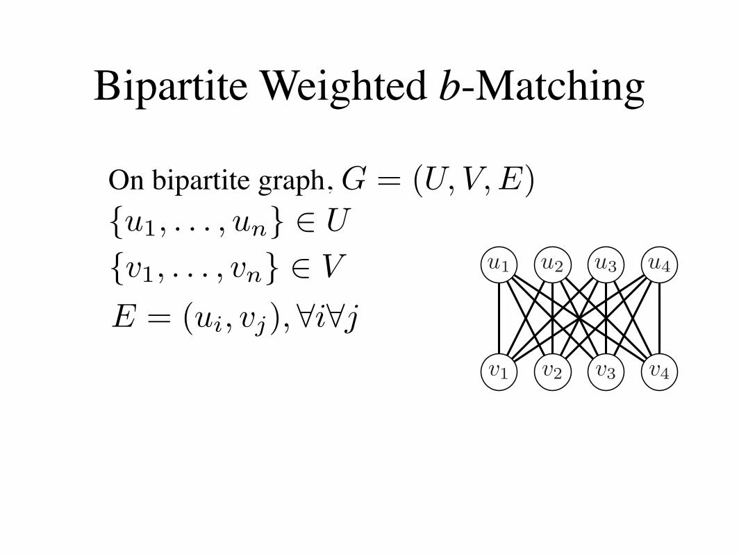
Bipartite Weighted b-Matching
Bipartite Weighted b-Matching
On bipartite graph, G = (U, V, E){u1, . . . , un} ! U
{v1, . . . , vn} ! V
E = (ui, vj),!i!j
Loopy Belief Propagation for Bipartite Maximum Weight b-Matching
Bert Huang
Computer Science Dept.Columbia UniversityNew York, NY 10027
Tony Jebara
Computer Science Dept.Columbia UniversityNew York, NY 10027
Abstract
We formulate the weighted b-matching ob-jective function as a probability distributionfunction and prove that belief propagation(BP) on its graphical model converges tothe optimum. Standard BP on our graphi-cal model cannot be computed in polynomialtime, but we introduce an algebraic methodto circumvent the combinatorial message up-dates. Empirically, the resulting algorithmis on average faster than popular combina-torial implementations, while still scaling atthe same asymptotic rate of O(bn3). Further-more, the algorithm shows promising perfor-mance in machine learning applications.
1 INTRODUCTION
u1 u2 u3 u4
v1 v2 v3 v4
Figure 1: Example b-matching MG on a bipartite graph G.Dashed lines represent possible edges, solid lines representb-matched edges. In this case b = 2.
2 EXPERIMENTS
We elaborate the speed advantages of our method andan application in machine learning where b-matchingcan improve classification accuracy.
2.1 RUNNING TIME ANALYSIS
We compare the performance of our implementationof belief propagation maximum weighted b-matching
u1 u2 u3 u4
v1 v2 v3 v4
1,5 234 6
Figure 3: The cyclic alternating path PG starting at v1 onG that corresponds to the nodes visited by PT . Edges arenumbered to help follow the loopy path.
against the free graph optimization package, GOBLIN.1
Classical b-matching algorithms such as the balancednetwork flow method used by the GOBLIN library runin O(bn3) time [?]. The belief propagation methodtakes O(bn) time to compute one iteration of messageupdates for each of the 2n nodes and converges in O(n)iterations. So, its overall running time is also O(bn3).
We ran both algorithms on randomly generated bipar-tite graphs of 10 ! n ! 100 and 1 ! b ! n/2. Wegenerated the weight matrix with the rand functionin MATLAB, which picks each weight independentlyfrom a uniform distribution between 0 and 1.
The GOBLIN library is C++ code and our implemen-tation2 of belief propagation b-matching is in C. Bothwere run on a 3.00 Ghz. Pentium 4 processor.
In general, the belief propagation runs hundreds oftimes faster than GOBLIN. Figure 5 shows variouscomparisons of their running times. The surface plotsshow how the algorithms scale with respect to n andb. The line plots show cross sections of these surfaceplots, with appropriate transformations on the run-ning time to show the scaling (without these transfor-mations, the belief propagation line would appear tobe always zero due to the scale of the plot following
1Available at: http://www.math.uni-augsburg.de/opt/goblin.html2Available at http://www.cs.columbia.edu/bert/bmatching
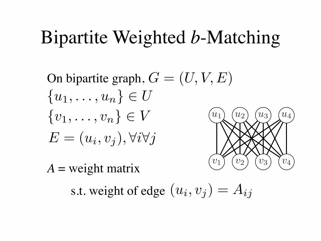
Bipartite Weighted b-Matching
On bipartite graph,
A = weight matrix
s.t. weight of edge
G = (U, V, E){u1, . . . , un} ! U
{v1, . . . , vn} ! V
E = (ui, vj),!i!j
(ui, vj) = Aij
Loopy Belief Propagation for Bipartite Maximum Weight b-Matching
Bert Huang
Computer Science Dept.Columbia UniversityNew York, NY 10027
Tony Jebara
Computer Science Dept.Columbia UniversityNew York, NY 10027
Abstract
We formulate the weighted b-matching ob-jective function as a probability distributionfunction and prove that belief propagation(BP) on its graphical model converges tothe optimum. Standard BP on our graphi-cal model cannot be computed in polynomialtime, but we introduce an algebraic methodto circumvent the combinatorial message up-dates. Empirically, the resulting algorithmis on average faster than popular combina-torial implementations, while still scaling atthe same asymptotic rate of O(bn3). Further-more, the algorithm shows promising perfor-mance in machine learning applications.
1 INTRODUCTION
u1 u2 u3 u4
v1 v2 v3 v4
Figure 1: Example b-matching MG on a bipartite graph G.Dashed lines represent possible edges, solid lines representb-matched edges. In this case b = 2.
2 EXPERIMENTS
We elaborate the speed advantages of our method andan application in machine learning where b-matchingcan improve classification accuracy.
2.1 RUNNING TIME ANALYSIS
We compare the performance of our implementationof belief propagation maximum weighted b-matching
u1 u2 u3 u4
v1 v2 v3 v4
1,5 234 6
Figure 3: The cyclic alternating path PG starting at v1 onG that corresponds to the nodes visited by PT . Edges arenumbered to help follow the loopy path.
against the free graph optimization package, GOBLIN.1
Classical b-matching algorithms such as the balancednetwork flow method used by the GOBLIN library runin O(bn3) time [?]. The belief propagation methodtakes O(bn) time to compute one iteration of messageupdates for each of the 2n nodes and converges in O(n)iterations. So, its overall running time is also O(bn3).
We ran both algorithms on randomly generated bipar-tite graphs of 10 ! n ! 100 and 1 ! b ! n/2. Wegenerated the weight matrix with the rand functionin MATLAB, which picks each weight independentlyfrom a uniform distribution between 0 and 1.
The GOBLIN library is C++ code and our implemen-tation2 of belief propagation b-matching is in C. Bothwere run on a 3.00 Ghz. Pentium 4 processor.
In general, the belief propagation runs hundreds oftimes faster than GOBLIN. Figure 5 shows variouscomparisons of their running times. The surface plotsshow how the algorithms scale with respect to n andb. The line plots show cross sections of these surfaceplots, with appropriate transformations on the run-ning time to show the scaling (without these transfor-mations, the belief propagation line would appear tobe always zero due to the scale of the plot following
1Available at: http://www.math.uni-augsburg.de/opt/goblin.html2Available at http://www.cs.columbia.edu/bert/bmatching
Bipartite Weighted b-Matching
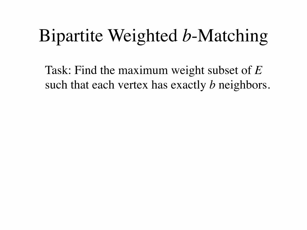
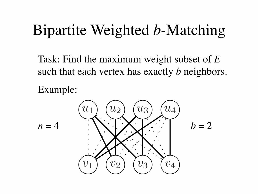
Task: Find the maximum weight subset of E such that each vertex has exactly b neighbors.
Bipartite Weighted b-Matching
Task: Find the maximum weight subset of E such that each vertex has exactly b neighbors.
Example:
n = 4 b = 2
Graphical models are powerful probabilistic construc-tions that describe the dependencies between di!erentdimensions in a probability distribution. In an acyclicgraph, a graphical model can be correctly maximizedor marginalized by collecting messages from all leafnodes at some root, then distributing messages backtoward the leaf nodes [7].
However, when loops are present in the graph, beliefpropagation methods often reach oscillation states orconverge to either local maxima or incorrect marginals.Cases with a single loop have been analyzed in[10], which gives an analytical expression relating thesteady-state beliefs to the true marginals.
Previous work related convergence of BP to types offree energy in [8], and [5] describes general su"cientconditions for convergence towards marginals.
Belief propagation has been generalized into a largerset of algorithms called tree-based reparameterization(TRP) in [9]. These algorithms iteratively reparam-eterize the distribution without changing it based onvarious trees in the original graph. Pairwise BP canbe interpreted as doing this on the two-node trees ofeach edge. The set of graphs on which TRP convergessubsumes that of BP. However, we use standard beliefpropagation here because it converges on our graph,it is simpler to implement and has additional benefitssuch as parallel computation.
In this work, we provide a proof of convergence basedon our specific graphical model and use the topologyof our graph to find our convergence time.
3 THE b-MATCHING GRAPHICALMODEL
u1 u2 u3 u4
v1 v2 v3 v4
Figure 1: Example b-matching MG on a bipartite graph G.Dashed lines represent possible edges, solid lines representb-matched edges. In this case b = 2.
Consider a bipartite graph G = (U, V, E) such thatU = {u1, . . . , un}, V = {v1, . . . , vn}, and E =(ui, vj), !i " {1, . . . , n}, !j " {1, . . . , n}. Let A bethe weight matrix of G such that the weight of edge(ui, vj) is Aij . Let a b-matching be characterized by afunction M(ui) or M(vj) that returns the set of neigh-bor vertices of the input vertex in the b-matching. Theb-matching objective function can then be written as
maxM
W(M) =
maxM
n!
i=1
!
vk!M(ui)
Aik +n
!
j=1
!
u!!M(vj)
A!j
s.t. |M(ui)| = b, !i " {1, . . . , n}|M(vj)| = b, !j " {1, . . . , n} .
(1)
If we define variables xi " X and yj " Y for eachvertex such that xi = M(ui), and yj = M(vj), we candefine the following functions:
!(xi) = exp(!
vj!xi
Aij), !(yj) = exp(!
ui!yj
Aij)
"(xi, yj) = ¬(vj " xi # ui " yj). (2)
Note that both X and Y have values over"
nb
#
con-figurations. For example, for n = 4 and b = 2, xi
could be any entry from {{1, 2}, {1, 3}, {1, 4}, {2, 3},{2, 4}, {3, 4}}. Similarly, if we were to crudely viewthe potential functions !(xi), !(yj) and "(xi, yj) as
tables, these tables would be of size"
nb
#
,"
nb
#
and"
nb
#2
entries respectively. The potential function "(xi, yj)is a binary function which goes to zero if yj containsa configuration that chooses node ui when xi does notcontain a configuration that includes node vj and vice-versa. These are zero configurations since they createan invalid b-matching. Otherwise "(xi, yj) = 1 if xi
and yj are in configurations that could agree with afeasible b-matching. In Section 3.2 we will show howto avoid ever directly manipulating these cumbersometables explicitly.
Using the potentials and pairwise clique functions, wecan write out the weighted b-matching objective as aprobability distribution p(X, Y ) $ exp(W(M)) [1].
p(X, Y ) =1
Z
n$
i=1
n$
j=1
"(xi, yj)n
$
k=1
!(xk)!(yk) (3)
3.1 THE MAX-PRODUCT ALGORITHM
We maximize this probability function using the max-product algorithm. The max-product algorithm iter-atively passes messages, which are vectors over set-tings of the variables, between dependent variables andstores beliefs, which are estimates of max-marginals.The following are the update equations for messagesfrom xi to yj. To avoid clutter, we omit the formu-las for messages from yj to xi because these updateequations for the reverse messages are the same ex-cept we swap the x and the y terms. In general, thedefault range of subscript indices is 1 through n; weonly indicate the exceptions.
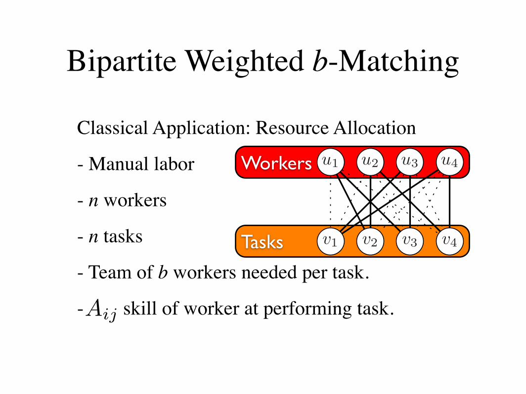
Classical Application: Resource Allocation
- Manual labor
- n workers
- n tasks
- Team of b workers needed per task.
- skill of worker at performing task.
Bipartite Weighted b-Matching
Aij
Tasks
Workers
Graphical models are powerful probabilistic construc-tions that describe the dependencies between di!erentdimensions in a probability distribution. In an acyclicgraph, a graphical model can be correctly maximizedor marginalized by collecting messages from all leafnodes at some root, then distributing messages backtoward the leaf nodes [7].
However, when loops are present in the graph, beliefpropagation methods often reach oscillation states orconverge to either local maxima or incorrect marginals.Cases with a single loop have been analyzed in[10], which gives an analytical expression relating thesteady-state beliefs to the true marginals.
Previous work related convergence of BP to types offree energy in [8], and [5] describes general su"cientconditions for convergence towards marginals.
Belief propagation has been generalized into a largerset of algorithms called tree-based reparameterization(TRP) in [9]. These algorithms iteratively reparam-eterize the distribution without changing it based onvarious trees in the original graph. Pairwise BP canbe interpreted as doing this on the two-node trees ofeach edge. The set of graphs on which TRP convergessubsumes that of BP. However, we use standard beliefpropagation here because it converges on our graph,it is simpler to implement and has additional benefitssuch as parallel computation.
In this work, we provide a proof of convergence basedon our specific graphical model and use the topologyof our graph to find our convergence time.
3 THE b-MATCHING GRAPHICALMODEL
u1 u2 u3 u4
v1 v2 v3 v4
Figure 1: Example b-matching MG on a bipartite graph G.Dashed lines represent possible edges, solid lines representb-matched edges. In this case b = 2.
Consider a bipartite graph G = (U, V, E) such thatU = {u1, . . . , un}, V = {v1, . . . , vn}, and E =(ui, vj), !i " {1, . . . , n}, !j " {1, . . . , n}. Let A bethe weight matrix of G such that the weight of edge(ui, vj) is Aij . Let a b-matching be characterized by afunction M(ui) or M(vj) that returns the set of neigh-bor vertices of the input vertex in the b-matching. Theb-matching objective function can then be written as
maxM
W(M) =
maxM
n!
i=1
!
vk!M(ui)
Aik +n
!
j=1
!
u!!M(vj)
A!j
s.t. |M(ui)| = b, !i " {1, . . . , n}|M(vj)| = b, !j " {1, . . . , n} .
(1)
If we define variables xi " X and yj " Y for eachvertex such that xi = M(ui), and yj = M(vj), we candefine the following functions:
!(xi) = exp(!
vj!xi
Aij), !(yj) = exp(!
ui!yj
Aij)
"(xi, yj) = ¬(vj " xi # ui " yj). (2)
Note that both X and Y have values over"
nb
#
con-figurations. For example, for n = 4 and b = 2, xi
could be any entry from {{1, 2}, {1, 3}, {1, 4}, {2, 3},{2, 4}, {3, 4}}. Similarly, if we were to crudely viewthe potential functions !(xi), !(yj) and "(xi, yj) as
tables, these tables would be of size"
nb
#
,"
nb
#
and"
nb
#2
entries respectively. The potential function "(xi, yj)is a binary function which goes to zero if yj containsa configuration that chooses node ui when xi does notcontain a configuration that includes node vj and vice-versa. These are zero configurations since they createan invalid b-matching. Otherwise "(xi, yj) = 1 if xi
and yj are in configurations that could agree with afeasible b-matching. In Section 3.2 we will show howto avoid ever directly manipulating these cumbersometables explicitly.
Using the potentials and pairwise clique functions, wecan write out the weighted b-matching objective as aprobability distribution p(X, Y ) $ exp(W(M)) [1].
p(X, Y ) =1
Z
n$
i=1
n$
j=1
"(xi, yj)n
$
k=1
!(xk)!(yk) (3)
3.1 THE MAX-PRODUCT ALGORITHM
We maximize this probability function using the max-product algorithm. The max-product algorithm iter-atively passes messages, which are vectors over set-tings of the variables, between dependent variables andstores beliefs, which are estimates of max-marginals.The following are the update equations for messagesfrom xi to yj. To avoid clutter, we omit the formu-las for messages from yj to xi because these updateequations for the reverse messages are the same ex-cept we swap the x and the y terms. In general, thedefault range of subscript indices is 1 through n; weonly indicate the exceptions.
Bipartite Weighted b-Matching
Alternate uses of b-matching:
- Balanced k-nearest-neighbors
- Each node can only be picked k times.
- Robust to translations of test data.
- When test data is collected under different conditions (e.g. time, location, instrument calibration).
Bipartite Weighted b-Matching
Classical algorithms solve Max-Weighted b-Matching in running time, such as:
- Blossom Algorithm (Edmonds 1965)
- Balanced Network Flow
(Fremuth-Paeger, Jungnickel 1999)
O(bn3)
1. Bipartite Weighted b-Matching
2. Edge Weights As a Distribution
3. Efficient Max-Product
4. Convergence Proof Sketch
5. Experiments
6. Discussion
Outline
Edge Weights As a Distribution
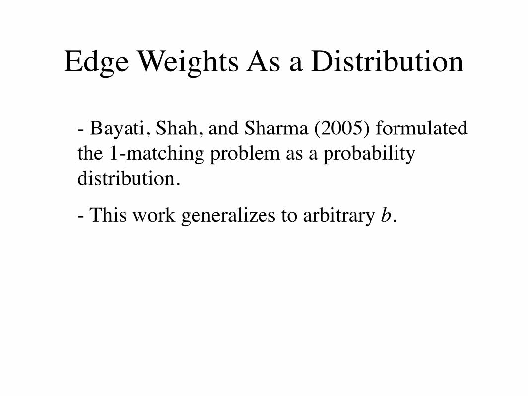
- Bayati, Shah, and Sharma (2005) formulated the 1-matching problem as a probability distribution.
- This work generalizes to arbitrary b.

Edge Weights As a Distribution
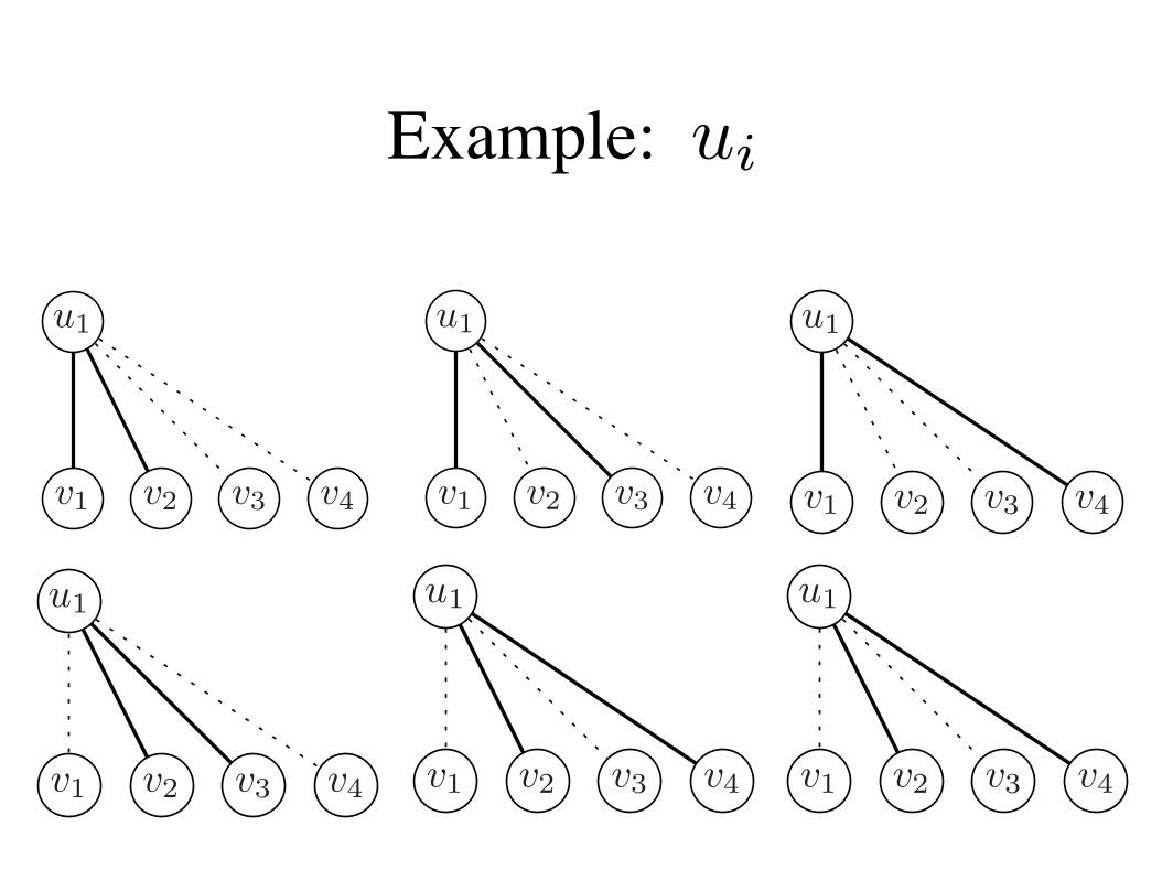
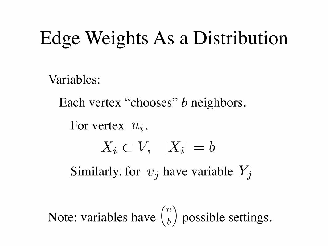
Variables:
Each vertex “chooses” b neighbors.
Loopy Belief Propagation for Bipartite Maximum Weight b-Matching
Bert Huang
Computer Science Dept.Columbia UniversityNew York, NY 10027
Tony Jebara
Computer Science Dept.Columbia UniversityNew York, NY 10027
Abstract
We formulate the weighted b-matching ob-jective function as a probability distributionfunction and prove that belief propagation(BP) on its graphical model converges tothe optimum. Standard BP on our graphi-cal model cannot be computed in polynomialtime, but we introduce an algebraic methodto circumvent the combinatorial message up-dates. Empirically, the resulting algorithmis on average faster than popular combina-torial implementations, while still scaling atthe same asymptotic rate of O(bn3). Further-more, the algorithm shows promising perfor-mance in machine learning applications.
1 INTRODUCTION
u1
v1 v2 v3 v4
u1
v1 v2 v3 v4
2 EXPERIMENTS
We elaborate the speed advantages of our method andan application in machine learning where b-matchingcan improve classification accuracy.
u1
v1 v2 v3 v4
u1
v1 v2 v3 v4
2.1 RUNNING TIME ANALYSIS
We compare the performance of our implementationof belief propagation maximum weighted b-matchingagainst the free graph optimization package, GOBLIN.1
Classical b-matching algorithms such as the balancednetwork flow method used by the GOBLIN library runin O(bn3) time [?]. The belief propagation methodtakes O(bn) time to compute one iteration of messageupdates for each of the 2n nodes and converges in O(n)iterations. So, its overall running time is also O(bn3).
We ran both algorithms on randomly generated bipar-tite graphs of 10 ! n ! 100 and 1 ! b ! n/2. Wegenerated the weight matrix with the rand functionin MATLAB, which picks each weight independently
1Available at: http://www.math.uni-augsburg.de/opt/goblin.html
u1
v1 v2 v3 v4
Example: -ui
Edge Weights As a Distribution
Variables:
Each vertex “chooses” b neighbors.
Edge Weights As a Distribution
Variables:
Each vertex “chooses” b neighbors.
For vertex ,
Similarly, for have variable
Note: variables have possible settings.
ui
vj
!
n
b
"
Xi ! V, |Xi| = b
Yj
Edge Weights As a Distribution
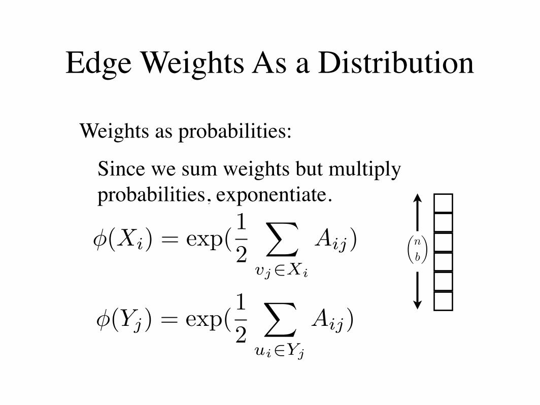
Weights as probabilities:
Since we sum weights but multiply probabilities, exponentiate.
!
n
b
"!(Xi) = exp(1
2
!
vj!Xi
Aij)
!(Yj) = exp(1
2
!
ui!Yj
Aij)

Edge Weights As a Distribution
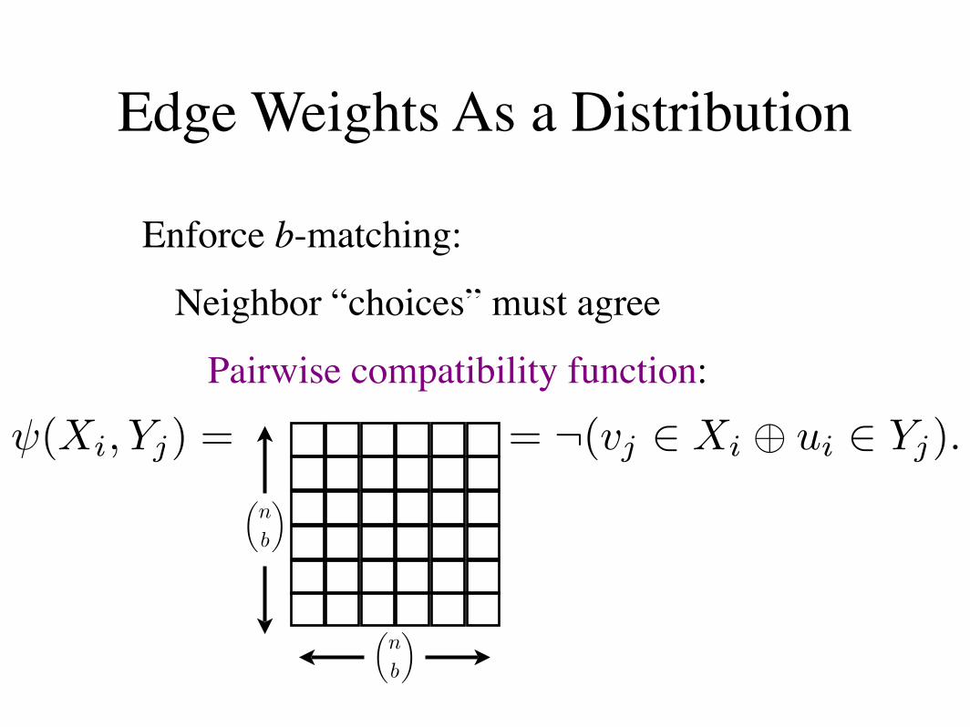
Enforce b-matching:
Neighbor “choices” must agree
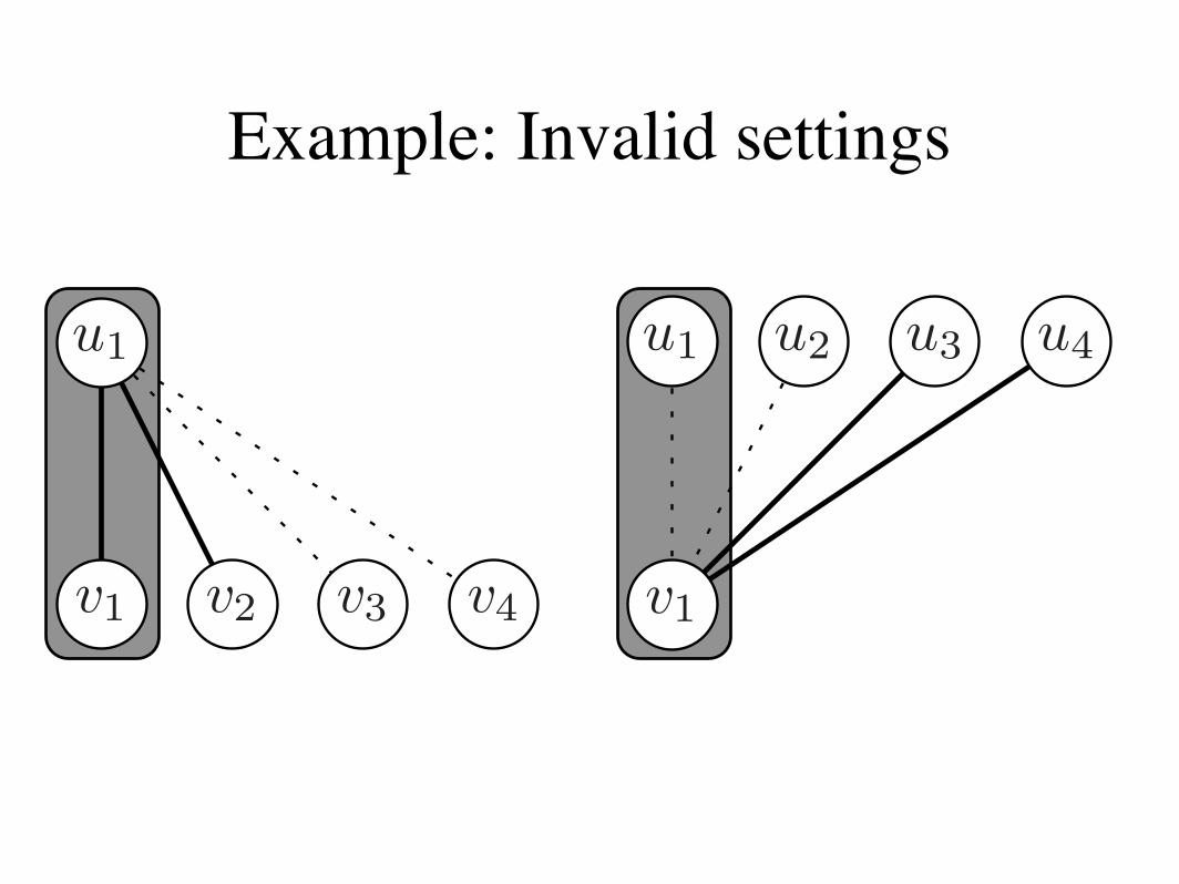
Example: Invalid settings
Loopy Belief Propagation for Bipartite Maximum Weight b-Matching
Bert Huang
Computer Science Dept.Columbia UniversityNew York, NY 10027
Tony Jebara
Computer Science Dept.Columbia UniversityNew York, NY 10027
Abstract
We formulate the weighted b-matching ob-jective function as a probability distributionfunction and prove that belief propagation(BP) on its graphical model converges tothe optimum. Standard BP on our graphi-cal model cannot be computed in polynomialtime, but we introduce an algebraic methodto circumvent the combinatorial message up-dates. Empirically, the resulting algorithmis on average faster than popular combina-torial implementations, while still scaling atthe same asymptotic rate of O(bn3). Further-more, the algorithm shows promising perfor-mance in machine learning applications.
1 INTRODUCTION
u1
v1 v2 v3 v4
u1
v1 v2 v3 v4
2 EXPERIMENTS
We elaborate the speed advantages of our method andan application in machine learning where b-matchingcan improve classification accuracy.
u1
v1 v2 v3 v4
u1
v1 v2 v3 v4
2.1 RUNNING TIME ANALYSIS
We compare the performance of our implementationof belief propagation maximum weighted b-matchingagainst the free graph optimization package, GOBLIN.1
Classical b-matching algorithms such as the balancednetwork flow method used by the GOBLIN library runin O(bn3) time [?]. The belief propagation methodtakes O(bn) time to compute one iteration of messageupdates for each of the 2n nodes and converges in O(n)iterations. So, its overall running time is also O(bn3).
We ran both algorithms on randomly generated bipar-tite graphs of 10 ! n ! 100 and 1 ! b ! n/2. Wegenerated the weight matrix with the rand functionin MATLAB, which picks each weight independently
1Available at: http://www.math.uni-augsburg.de/opt/goblin.html
u1
v1 v2 v3 v4
u1
v1 v2 v3 v4
u2 u2 u2 u2u3 u3 u3 u3u4 u4 u4 u4
v2 v3 v4 v2 v3 v4 v2 v3 v4 v1 v3 v4 v1 v3 v4 v1 v3 v4 v1 v2 v4 v1 v2 v4 v1 v2 v4 v1 v2 v3 v1 v2 v3 v1 v2 v3
Figure 4: Example unwrapped graph T of G at 3 iterations. The matching MT is highlighted based on MG from Figure2. Note that leaf nodes cannot have perfect b-matchings, but all inner nodes and the root do. One possible path PT ishighlighted, which is discussed in Lemma ??.
. . .u2v2u4v1u1v3u4v1u3
First cycle
(a) PG
u4
v3u1
v1
(b) c1
. . .u2v2u4v1u3
(c) PG \ c1
Figure 6: (a) One possible extension of PG from Figure 1. This path comes from a deeper T so PG is longer. The firstcycle c1 detected is highlighted. (b) Cycle c1 from PG. (c) The remainder of PG when we remove c1. Note the alternationof the matched edges remains consistent even when we cut out cycles in the interior of the path.
u1
v1 v2 v3 v4
u1 u2 u3 u4
v1 v2 v3 v4
Figure 1: Example b-matching MG on a bipartite graph G.Dashed lines represent possible edges, solid lines representb-matched edges. In this case b = 2.
from a uniform distribution between 0 and 1.
The GOBLIN library is C++ code and our implemen-tation2 of belief propagation b-matching is in C. Bothwere run on a 3.00 Ghz. Pentium 4 processor.
In general, the belief propagation runs hundreds oftimes faster than GOBLIN. Figure 6 shows variouscomparisons of their running times. The surface plotsshow how the algorithms scale with respect to n andb. The line plots show cross sections of these surfaceplots, with appropriate transformations on the run-ning time to show the scaling (without these transfor-mations, the belief propagation line would appear to
2Available at http://www.cs.columbia.edu/bert/bmatching
u1 u2 u3 u4
v1
Figure 2: Example b-matching MG on a bipartite graph G.Dashed lines represent possible edges, solid lines representb-matched edges. In this case b = 2.
u1 u2 u3 u4
v1 v2 v3 v4
Figure 3: Example b-matching MG on a bipartite graph G.Dashed lines represent possible edges, solid lines representb-matched edges. In this case b = 2.
be always zero due to the scale of the plot followingthe GOBLIN line). Since both algorithms have run-ning time O(bn3), when we fix b = 5, we get a cubiccurve. When we fix b = n/2, we get a quartic curvebecause b becomes a function of n.
2.2 b-MATCHING FOR CLASSIFICATION
One natural application of b-matching is as an im-provement over k-nearest neighbor (KNN) for classi-fication. Using KNN for classification is a quick way
Edge Weights As a Distribution
Enforce b-matching:
Neighbor “choices” must agree
Edge Weights As a Distribution
Enforce b-matching:
Neighbor “choices” must agree
Pairwise compatibility function:
= ¬(vj ! Xi " ui ! Yj).
!
n
b
"
!
n
b
"
!(Xi, Yj) =
Edge Weights As a Distribution
!(Xi) = exp(1
2
!
vj!Xi
Aij) !(Yj) = exp(1
2
!
ui!Yj
Aij)
!(Xi, Yj) = ¬(vj ! Xi " ui ! Yj).
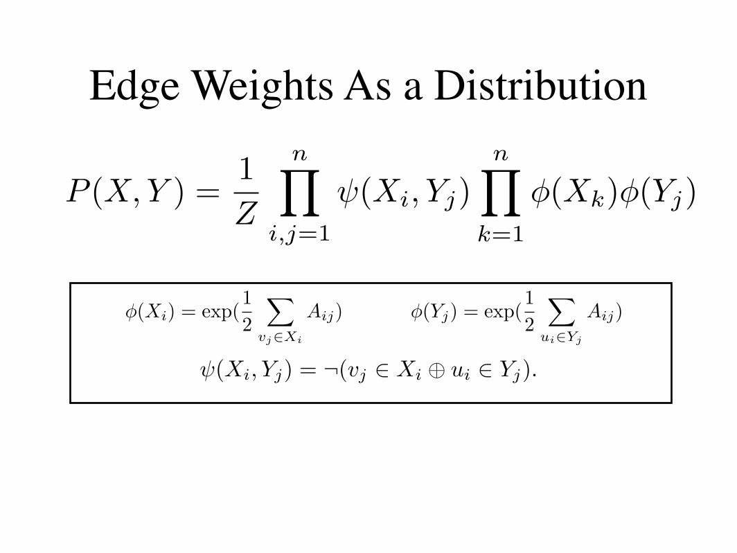
P (X, Y ) =1
Z
n!
i,j=1
!(Xi, Yj)n!
k=1
"(Xk)"(Yj)
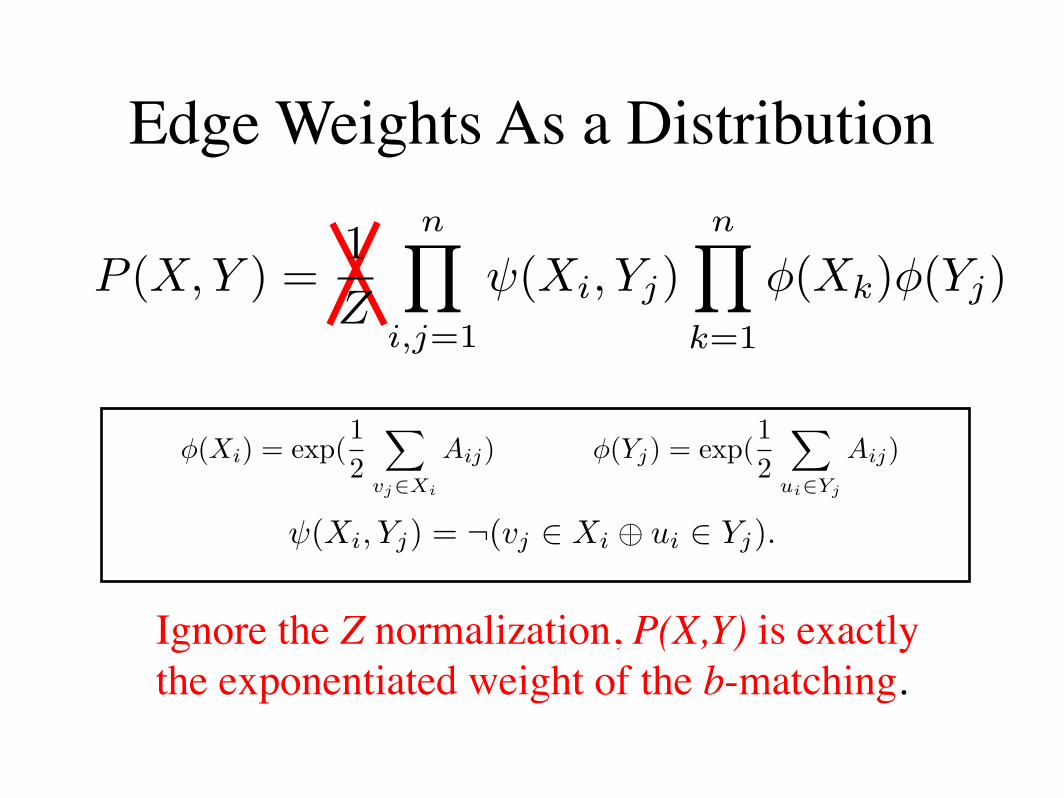
Edge Weights As a Distribution
Ignore the Z normalization, P(X,Y) is exactly the exponentiated weight of the b-matching.
!(Xi) = exp(1
2
!
vj!Xi
Aij) !(Yj) = exp(1
2
!
ui!Yj
Aij)
!(Xi, Yj) = ¬(vj ! Xi " ui ! Yj).
P (X, Y ) =1
Z
n!
i,j=1
!(Xi, Yj)n!
k=1
"(Xk)"(Yj)
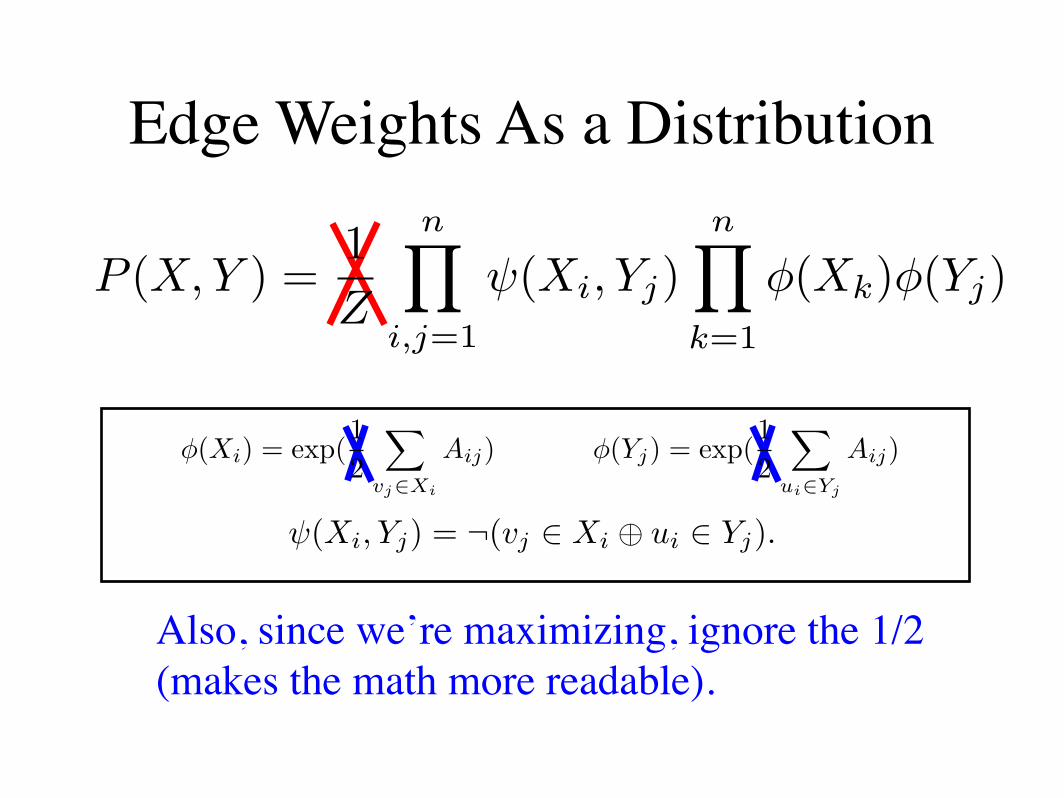
Edge Weights As a Distribution
Also, since we’re maximizing, ignore the 1/2 (makes the math more readable).
!(Xi) = exp(1
2
!
vj!Xi
Aij) !(Yj) = exp(1
2
!
ui!Yj
Aij)
!(Xi, Yj) = ¬(vj ! Xi " ui ! Yj).
P (X, Y ) =1
Z
n!
i,j=1
!(Xi, Yj)n!
k=1
"(Xk)"(Yj)
1. Bipartite Weighted b-Matching
2. Edge Weights As a Distribution
3. Efficient Max-Product
4. Convergence Proof Sketch
5. Experiments
6. Discussion
Outline
Standard Max-Product
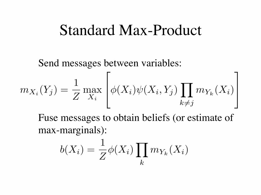
Send messages between variables:
Fuse messages to obtain beliefs (or estimate of max-marginals):
mXi(Yj) =
1
ZmaxXi
!
"!(Xi)"(Xi, Yj)#
k !=j
mYk(Xi)
$
%
b(Xi) =1
Z!(Xi)
!
k
mYk(Xi)

Standard Max-Product
Converges to true maximum on any tree structured graph (Pearl 1986).
We show that it converges to the correct maximum on our graph.

Standard Max-Product
Converges to true maximum on any tree structured graph (Pearl 1986).
We show that it converges to the correct maximum on our graph.
But what about the -length message and belief vectors?
!
n
b
"
Efficient Max-Product
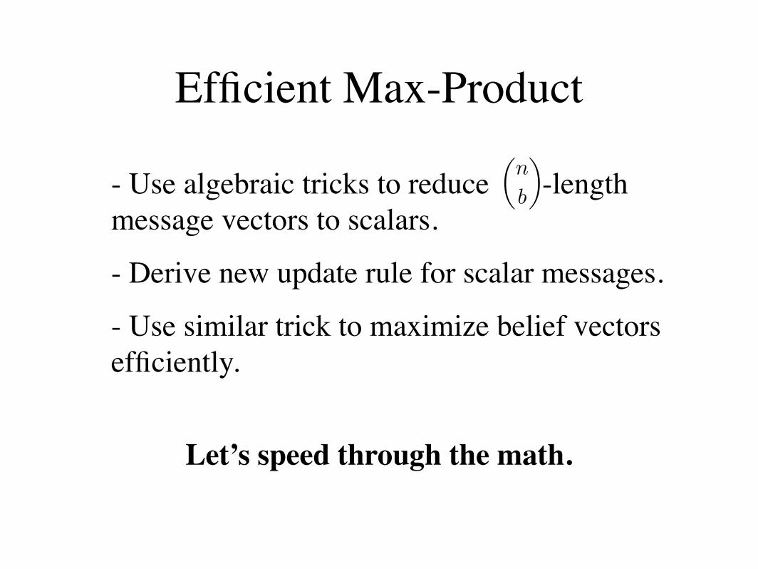
- Use algebraic tricks to reduce -length message vectors to scalars.
- Derive new update rule for scalar messages.
- Use similar trick to maximize belief vectors efficiently.
!
n
b
"
Let’s speed through the math.
Efficient Max-Product
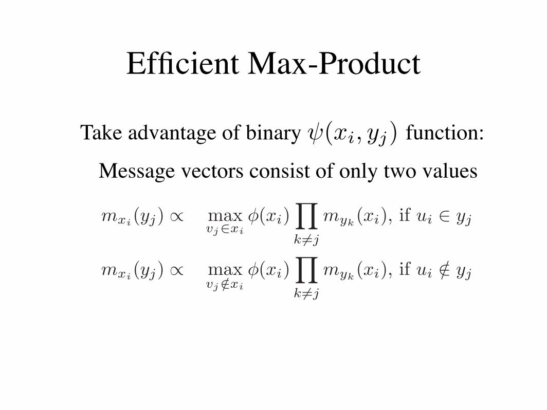
Take advantage of binary function:
Message vectors consist of only two values
!(xi, yj)
mxi(yj) =1
Zmax
xi
!
"!(xi)"(xi, yj)#
k !=j
myk(xi)
$
%
b(xi) =1
Z!(xi)
#
k
myk(xi)
Loopy belief propagation on this graph converges tothe optimum. However, since there are
&
nb
'
possiblesettings for each variable, direct belief propagation isnot feasible with larger graphs.
3.2 EFFICIENT BELIEF PROPAGATIONOF
&
nb
'
-LENGTH MESSAGE VECTORS
We exploit three peculiarities of the above formulationto fully represent the
&nb
'
length messages as scalars.
First, the " functions are well structured, and theirstructure causes the maximization term in the messageupdates to always be one of two values.
mxi(yj) ! maxvj"xi
!(xi)#
k !=j
myk(xi), if ui " yj
mxi(yj) ! maxvj /"xi
!(xi)#
k !=j
myk(xi), if ui /" yj (4)
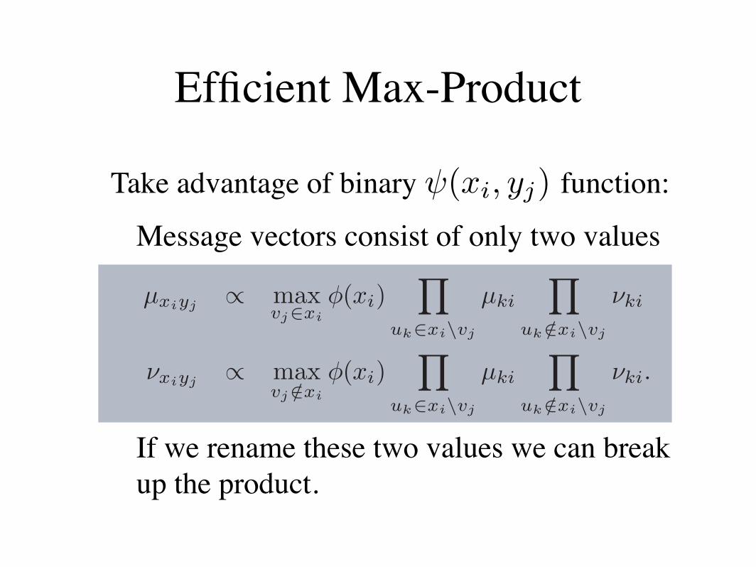
This is because the " function changes based only onwhether the setting of yj indicates that vj shares anedge with ui. Furthermore, if we redefine the abovemessage values as two scalars, we can write the mes-sages more specifically as
µxiyj ! maxvj"xi
!(xi)#
uk"xi\vj
µki
#
uk /"xi\vj
#ki
#xiyj ! maxvj /"xi
!(xi)#
uk"xi\vj
µki
#
uk /"xi\vj
#ki. (5)
Second, since the messages are unnormalized proba-bilities, we can divide any constant from the vectorswithout changing the result. We divide all entries inthe message vector by #xiyj to get
µxiyj =µxiyj
#xiyj
and #xiyj = 1 .
This lossless compression scheme simplifies the storageof message vectors from length
&
nb
'
to 1.
We rewrite the ! functions as a product of the expo-nentiated Aij weights and eliminate the need to ex-haustively maximize over all possible sets of size b. In-serting Equation (2) into the definition of µxiyj gives
µxiyj =maxj"xi !(xi)
(
k"xi\j µki
maxj /"xi!(xi)
(
k"xi\j µki
=maxj"xi
(
k"xiexp(Aik)
(
k"xi\j µki
maxj /"xi
(
k"xiexp(Aik)
(
k"xi\j µki
=exp(Aij)maxj"xi
(
k"xi\j exp(Aik)µki
maxj /"xi
(
k"xiexp(Aij)µki
(6)
We cancel out common terms and are left with thesimple message update rule,
µxiyj =exp(Aij)
exp(Ai!)µy!xi
.
Here, the index $ refers to the the bth greatest set-ting of k for the term exp(Aik)myk(xi), where k #= j.This compressed version of a message update can becomputed in O(bn) time.
We cannot e!ciently reconstruct the entire belief vec-tor but we can e!ciently find its maximum.
maxxi
b(xi) ! maxxi
!(xi)#
k"xi
µykxi
! maxxi
#
k"xi
exp(Aik)µykxi (7)
Finally, to maximize over xi we enumerate k andgreedily select the b largest values of exp(Aik)µykxi .
The above procedure avoids enumerating all&n
b
'
en-tries in the belief vector, and instead reshapes the dis-tribution into a b dimensional hypercube. The maxi-mum of the hypercube is found e!ciently by searchingeach dimension independently. Note that each dimen-sion represents one of the b edges for node ui.
4 PROOF OF CONVERGENCE
We begin with the assumption that MG, the maxi-mum weight b-matching on G, is unique. Moreover,W(MG), the weight of MG, is greater than that of anyother matching by a constant %.
% = W(MG) $ maxM !=MG
W(M)
Let T be the unwrapped graph of G from node ui. Anunwrapped graph is a tree that contains representa-tions of all paths of length d in G originating from asingle root node without any backtracking. Each nodein T maps to a corresponding node in G, and each nodein G maps to multiple nodes in T . Nodes and edges inT have the same local connectivity and potential func-tions as their corresponding nodes in G. Let r be theroot of T that corresponds to ui in the original graph

Efficient Max-Product
Take advantage of binary function:
Message vectors consist of only two values
If we rename these two values we can break up the product.
!(xi, yj)
mxi(yj) =1
Zmax
xi
!
"!(xi)"(xi, yj)#
k !=j
myk(xi)
$
%
b(xi) =1
Z!(xi)
#
k
myk(xi)
Loopy belief propagation on this graph converges tothe optimum. However, since there are
&
nb
'
possiblesettings for each variable, direct belief propagation isnot feasible with larger graphs.
3.2 EFFICIENT BELIEF PROPAGATIONOF
&
nb
'
-LENGTH MESSAGE VECTORS
We exploit three peculiarities of the above formulationto fully represent the
&nb
'
length messages as scalars.
First, the " functions are well structured, and theirstructure causes the maximization term in the messageupdates to always be one of two values.
mxi(yj) ! maxvj"xi
!(xi)#
k !=j
myk(xi), if ui " yj
mxi(yj) ! maxvj /"xi
!(xi)#
k !=j
myk(xi), if ui /" yj (4)
This is because the " function changes based only onwhether the setting of yj indicates that vj shares anedge with ui. Furthermore, if we redefine the abovemessage values as two scalars, we can write the mes-sages more specifically as
µxiyj ! maxvj"xi
!(xi)#
uk"xi\vj
µki
#
uk /"xi\vj
#ki
#xiyj ! maxvj /"xi
!(xi)#
uk"xi\vj
µki
#
uk /"xi\vj
#ki. (5)
Second, since the messages are unnormalized proba-bilities, we can divide any constant from the vectorswithout changing the result. We divide all entries inthe message vector by #xiyj to get
µxiyj =µxiyj
#xiyj
and #xiyj = 1 .
This lossless compression scheme simplifies the storageof message vectors from length
&
nb
'
to 1.
We rewrite the ! functions as a product of the expo-nentiated Aij weights and eliminate the need to ex-haustively maximize over all possible sets of size b. In-serting Equation (2) into the definition of µxiyj gives
µxiyj =maxj"xi !(xi)
(
k"xi\j µki
maxj /"xi!(xi)
(
k"xi\j µki
=maxj"xi
(
k"xiexp(Aik)
(
k"xi\j µki
maxj /"xi
(
k"xiexp(Aik)
(
k"xi\j µki
=exp(Aij)maxj"xi
(
k"xi\j exp(Aik)µki
maxj /"xi
(
k"xiexp(Aij)µki
(6)
We cancel out common terms and are left with thesimple message update rule,
µxiyj =exp(Aij)
exp(Ai!)µy!xi
.
Here, the index $ refers to the the bth greatest set-ting of k for the term exp(Aik)myk(xi), where k #= j.This compressed version of a message update can becomputed in O(bn) time.
We cannot e!ciently reconstruct the entire belief vec-tor but we can e!ciently find its maximum.
maxxi
b(xi) ! maxxi
!(xi)#
k"xi
µykxi
! maxxi
#
k"xi
exp(Aik)µykxi (7)
Finally, to maximize over xi we enumerate k andgreedily select the b largest values of exp(Aik)µykxi .
The above procedure avoids enumerating all&n
b
'
en-tries in the belief vector, and instead reshapes the dis-tribution into a b dimensional hypercube. The maxi-mum of the hypercube is found e!ciently by searchingeach dimension independently. Note that each dimen-sion represents one of the b edges for node ui.
4 PROOF OF CONVERGENCE
We begin with the assumption that MG, the maxi-mum weight b-matching on G, is unique. Moreover,W(MG), the weight of MG, is greater than that of anyother matching by a constant %.
% = W(MG) $ maxM !=MG
W(M)
Let T be the unwrapped graph of G from node ui. Anunwrapped graph is a tree that contains representa-tions of all paths of length d in G originating from asingle root node without any backtracking. Each nodein T maps to a corresponding node in G, and each nodein G maps to multiple nodes in T . Nodes and edges inT have the same local connectivity and potential func-tions as their corresponding nodes in G. Let r be theroot of T that corresponds to ui in the original graph
Efficient Max-Product
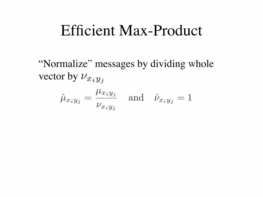
“Normalize” messages by dividing whole vector by
mxi(yj) =1
Zmax
xi
!
"!(xi)"(xi, yj)#
k !=j
myk(xi)
$
%
b(xi) =1
Z!(xi)
#
k
myk(xi)
Loopy belief propagation on this graph converges tothe optimum. However, since there are
&
nb
'
possiblesettings for each variable, direct belief propagation isnot feasible with larger graphs.
3.2 EFFICIENT BELIEF PROPAGATIONOF
&
nb
'
-LENGTH MESSAGE VECTORS
We exploit three peculiarities of the above formulationto fully represent the
&nb
'
length messages as scalars.
First, the " functions are well structured, and theirstructure causes the maximization term in the messageupdates to always be one of two values.
mxi(yj) ! maxvj"xi
!(xi)#
k !=j
myk(xi), if ui " yj
mxi(yj) ! maxvj /"xi
!(xi)#
k !=j
myk(xi), if ui /" yj (4)
This is because the " function changes based only onwhether the setting of yj indicates that vj shares anedge with ui. Furthermore, if we redefine the abovemessage values as two scalars, we can write the mes-sages more specifically as
µxiyj ! maxvj"xi
!(xi)#
uk"xi\vj
µki
#
uk /"xi\vj
#ki
#xiyj ! maxvj /"xi
!(xi)#
uk"xi\vj
µki
#
uk /"xi\vj
#ki. (5)
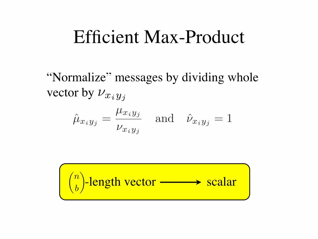
Second, since the messages are unnormalized proba-bilities, we can divide any constant from the vectorswithout changing the result. We divide all entries inthe message vector by #xiyj to get
µxiyj =µxiyj
#xiyj
and #xiyj = 1 .
This lossless compression scheme simplifies the storageof message vectors from length
&
nb
'
to 1.
We rewrite the ! functions as a product of the expo-nentiated Aij weights and eliminate the need to ex-haustively maximize over all possible sets of size b. In-serting Equation (2) into the definition of µxiyj gives
µxiyj =maxj"xi !(xi)
(
k"xi\j µki
maxj /"xi!(xi)
(
k"xi\j µki
=maxj"xi
(
k"xiexp(Aik)
(
k"xi\j µki
maxj /"xi
(
k"xiexp(Aik)
(
k"xi\j µki
=exp(Aij)maxj"xi
(
k"xi\j exp(Aik)µki
maxj /"xi
(
k"xiexp(Aij)µki
(6)
We cancel out common terms and are left with thesimple message update rule,
µxiyj =exp(Aij)
exp(Ai!)µy!xi
.
Here, the index $ refers to the the bth greatest set-ting of k for the term exp(Aik)myk(xi), where k #= j.This compressed version of a message update can becomputed in O(bn) time.
We cannot e!ciently reconstruct the entire belief vec-tor but we can e!ciently find its maximum.
maxxi
b(xi) ! maxxi
!(xi)#
k"xi
µykxi
! maxxi
#
k"xi
exp(Aik)µykxi (7)
Finally, to maximize over xi we enumerate k andgreedily select the b largest values of exp(Aik)µykxi .
The above procedure avoids enumerating all&n
b
'
en-tries in the belief vector, and instead reshapes the dis-tribution into a b dimensional hypercube. The maxi-mum of the hypercube is found e!ciently by searchingeach dimension independently. Note that each dimen-sion represents one of the b edges for node ui.
4 PROOF OF CONVERGENCE
We begin with the assumption that MG, the maxi-mum weight b-matching on G, is unique. Moreover,W(MG), the weight of MG, is greater than that of anyother matching by a constant %.
% = W(MG) $ maxM !=MG
W(M)
Let T be the unwrapped graph of G from node ui. Anunwrapped graph is a tree that contains representa-tions of all paths of length d in G originating from asingle root node without any backtracking. Each nodein T maps to a corresponding node in G, and each nodein G maps to multiple nodes in T . Nodes and edges inT have the same local connectivity and potential func-tions as their corresponding nodes in G. Let r be theroot of T that corresponds to ui in the original graph
!xiyj
Efficient Max-Product
“Normalize” messages by dividing whole vector by
-length vector scalar
mxi(yj) =1
Zmax
xi
!
"!(xi)"(xi, yj)#
k !=j
myk(xi)
$
%
b(xi) =1
Z!(xi)
#
k
myk(xi)
Loopy belief propagation on this graph converges tothe optimum. However, since there are
&
nb
'
possiblesettings for each variable, direct belief propagation isnot feasible with larger graphs.
3.2 EFFICIENT BELIEF PROPAGATIONOF
&
nb
'
-LENGTH MESSAGE VECTORS
We exploit three peculiarities of the above formulationto fully represent the
&nb
'
length messages as scalars.
First, the " functions are well structured, and theirstructure causes the maximization term in the messageupdates to always be one of two values.
mxi(yj) ! maxvj"xi
!(xi)#
k !=j
myk(xi), if ui " yj
mxi(yj) ! maxvj /"xi
!(xi)#
k !=j
myk(xi), if ui /" yj (4)
This is because the " function changes based only onwhether the setting of yj indicates that vj shares anedge with ui. Furthermore, if we redefine the abovemessage values as two scalars, we can write the mes-sages more specifically as
µxiyj ! maxvj"xi
!(xi)#
uk"xi\vj
µki
#
uk /"xi\vj
#ki
#xiyj ! maxvj /"xi
!(xi)#
uk"xi\vj
µki
#
uk /"xi\vj
#ki. (5)
Second, since the messages are unnormalized proba-bilities, we can divide any constant from the vectorswithout changing the result. We divide all entries inthe message vector by #xiyj to get
µxiyj =µxiyj
#xiyj
and #xiyj = 1 .
This lossless compression scheme simplifies the storageof message vectors from length
&
nb
'
to 1.
We rewrite the ! functions as a product of the expo-nentiated Aij weights and eliminate the need to ex-haustively maximize over all possible sets of size b. In-serting Equation (2) into the definition of µxiyj gives
µxiyj =maxj"xi !(xi)
(
k"xi\j µki
maxj /"xi!(xi)
(
k"xi\j µki
=maxj"xi
(
k"xiexp(Aik)
(
k"xi\j µki
maxj /"xi
(
k"xiexp(Aik)
(
k"xi\j µki
=exp(Aij)maxj"xi
(
k"xi\j exp(Aik)µki
maxj /"xi
(
k"xiexp(Aij)µki
(6)
We cancel out common terms and are left with thesimple message update rule,
µxiyj =exp(Aij)
exp(Ai!)µy!xi
.
Here, the index $ refers to the the bth greatest set-ting of k for the term exp(Aik)myk(xi), where k #= j.This compressed version of a message update can becomputed in O(bn) time.
We cannot e!ciently reconstruct the entire belief vec-tor but we can e!ciently find its maximum.
maxxi
b(xi) ! maxxi
!(xi)#
k"xi
µykxi
! maxxi
#
k"xi
exp(Aik)µykxi (7)
Finally, to maximize over xi we enumerate k andgreedily select the b largest values of exp(Aik)µykxi .
The above procedure avoids enumerating all&n
b
'
en-tries in the belief vector, and instead reshapes the dis-tribution into a b dimensional hypercube. The maxi-mum of the hypercube is found e!ciently by searchingeach dimension independently. Note that each dimen-sion represents one of the b edges for node ui.
4 PROOF OF CONVERGENCE
We begin with the assumption that MG, the maxi-mum weight b-matching on G, is unique. Moreover,W(MG), the weight of MG, is greater than that of anyother matching by a constant %.
% = W(MG) $ maxM !=MG
W(M)
Let T be the unwrapped graph of G from node ui. Anunwrapped graph is a tree that contains representa-tions of all paths of length d in G originating from asingle root node without any backtracking. Each nodein T maps to a corresponding node in G, and each nodein G maps to multiple nodes in T . Nodes and edges inT have the same local connectivity and potential func-tions as their corresponding nodes in G. Let r be theroot of T that corresponds to ui in the original graph
!xiyj
!
n
b
"
Efficient Max-Product
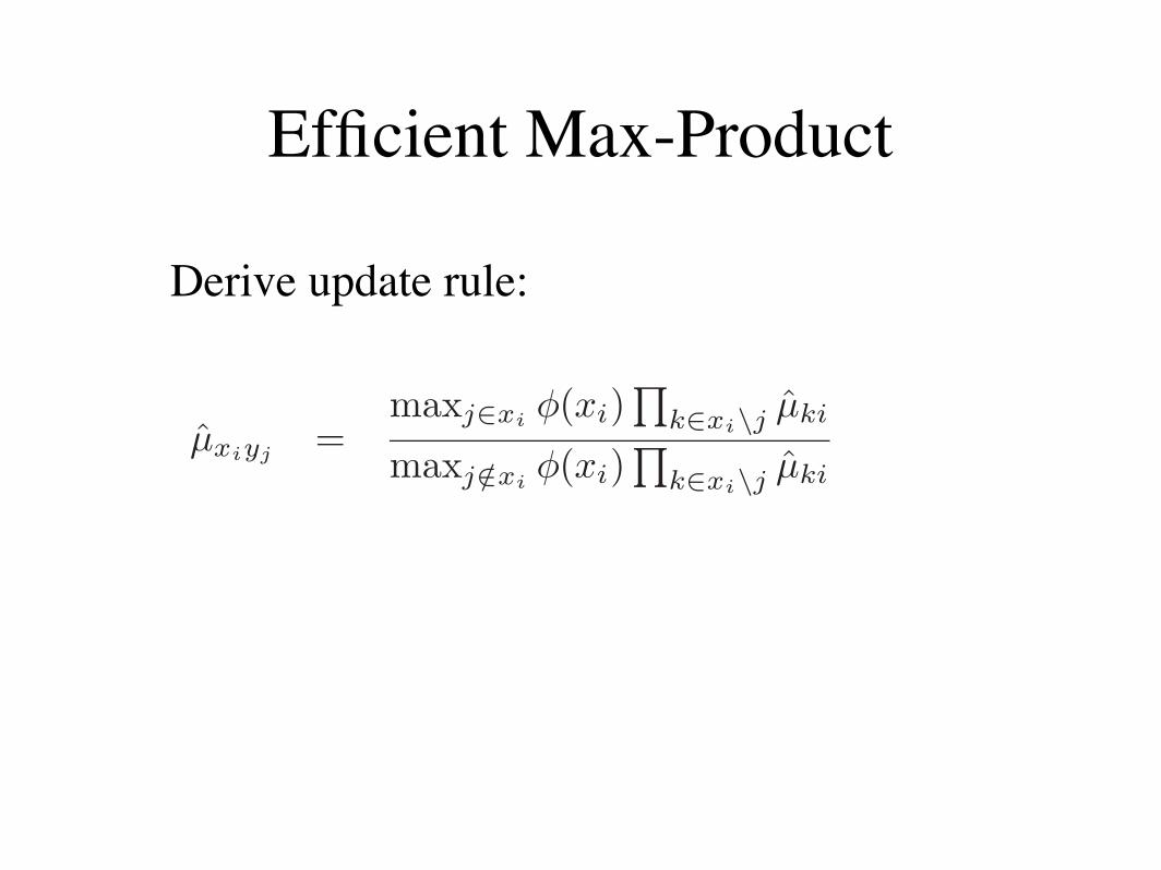
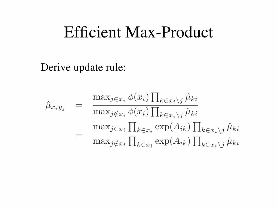
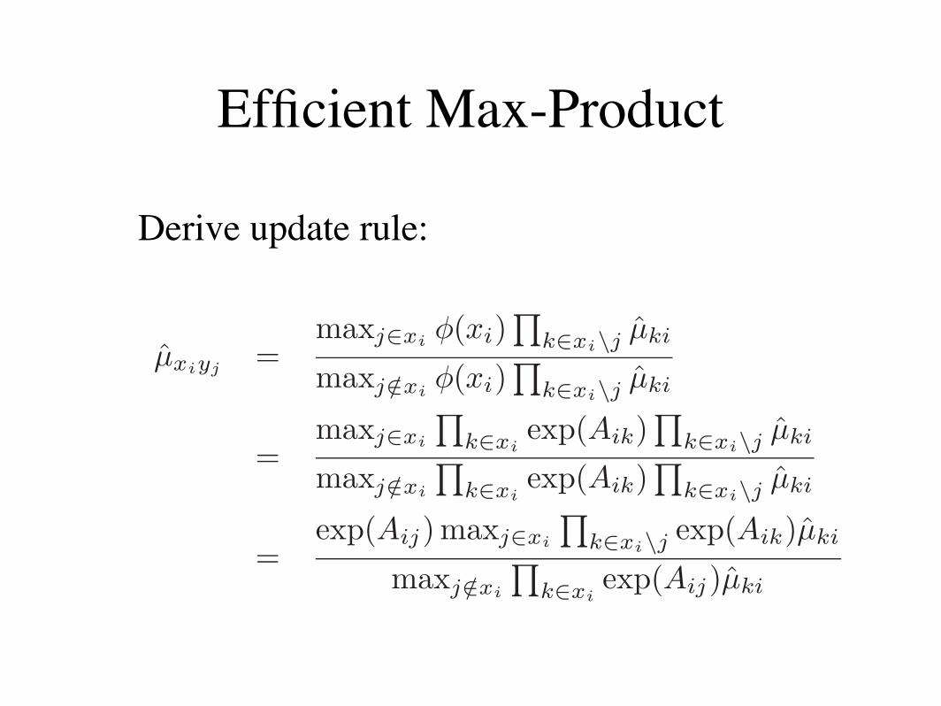
Derive update rule:
mxi(yj) =1
Zmax
xi
!
"!(xi)"(xi, yj)#
k !=j
myk(xi)
$
%
b(xi) =1
Z!(xi)
#
k
myk(xi)
Loopy belief propagation on this graph converges tothe optimum. However, since there are
&
nb
'
possiblesettings for each variable, direct belief propagation isnot feasible with larger graphs.
3.2 EFFICIENT BELIEF PROPAGATIONOF
&
nb
'
-LENGTH MESSAGE VECTORS
We exploit three peculiarities of the above formulationto fully represent the
&nb
'
length messages as scalars.
First, the " functions are well structured, and theirstructure causes the maximization term in the messageupdates to always be one of two values.
mxi(yj) ! maxvj"xi
!(xi)#
k !=j
myk(xi), if ui " yj
mxi(yj) ! maxvj /"xi
!(xi)#
k !=j
myk(xi), if ui /" yj (4)
This is because the " function changes based only onwhether the setting of yj indicates that vj shares anedge with ui. Furthermore, if we redefine the abovemessage values as two scalars, we can write the mes-sages more specifically as
µxiyj ! maxvj"xi
!(xi)#
uk"xi\vj
µki
#
uk /"xi\vj
#ki
#xiyj ! maxvj /"xi
!(xi)#
uk"xi\vj
µki
#
uk /"xi\vj
#ki. (5)
Second, since the messages are unnormalized proba-bilities, we can divide any constant from the vectorswithout changing the result. We divide all entries inthe message vector by #xiyj to get
µxiyj =µxiyj
#xiyj
and #xiyj = 1 .
This lossless compression scheme simplifies the storageof message vectors from length
&
nb
'
to 1.
We rewrite the ! functions as a product of the expo-nentiated Aij weights and eliminate the need to ex-haustively maximize over all possible sets of size b. In-serting Equation (2) into the definition of µxiyj gives
µxiyj =maxj"xi !(xi)
(
k"xi\j µki
maxj /"xi!(xi)
(
k"xi\j µki
=maxj"xi
(
k"xiexp(Aik)
(
k"xi\j µki
maxj /"xi
(
k"xiexp(Aik)
(
k"xi\j µki
=exp(Aij)maxj"xi
(
k"xi\j exp(Aik)µki
maxj /"xi
(
k"xiexp(Aij)µki
(6)
We cancel out common terms and are left with thesimple message update rule,
µxiyj =exp(Aij)
exp(Ai!)µy!xi
.
Here, the index $ refers to the the bth greatest set-ting of k for the term exp(Aik)myk(xi), where k #= j.This compressed version of a message update can becomputed in O(bn) time.
We cannot e!ciently reconstruct the entire belief vec-tor but we can e!ciently find its maximum.
maxxi
b(xi) ! maxxi
!(xi)#
k"xi
µykxi
! maxxi
#
k"xi
exp(Aik)µykxi (7)
Finally, to maximize over xi we enumerate k andgreedily select the b largest values of exp(Aik)µykxi .
The above procedure avoids enumerating all&n
b
'
en-tries in the belief vector, and instead reshapes the dis-tribution into a b dimensional hypercube. The maxi-mum of the hypercube is found e!ciently by searchingeach dimension independently. Note that each dimen-sion represents one of the b edges for node ui.
4 PROOF OF CONVERGENCE
We begin with the assumption that MG, the maxi-mum weight b-matching on G, is unique. Moreover,W(MG), the weight of MG, is greater than that of anyother matching by a constant %.
% = W(MG) $ maxM !=MG
W(M)
Let T be the unwrapped graph of G from node ui. Anunwrapped graph is a tree that contains representa-tions of all paths of length d in G originating from asingle root node without any backtracking. Each nodein T maps to a corresponding node in G, and each nodein G maps to multiple nodes in T . Nodes and edges inT have the same local connectivity and potential func-tions as their corresponding nodes in G. Let r be theroot of T that corresponds to ui in the original graph
Efficient Max-Product
Derive update rule:
mxi(yj) =1
Zmax
xi
!
"!(xi)"(xi, yj)#
k !=j
myk(xi)
$
%
b(xi) =1
Z!(xi)
#
k
myk(xi)
Loopy belief propagation on this graph converges tothe optimum. However, since there are
&
nb
'
possiblesettings for each variable, direct belief propagation isnot feasible with larger graphs.
3.2 EFFICIENT BELIEF PROPAGATIONOF
&
nb
'
-LENGTH MESSAGE VECTORS
We exploit three peculiarities of the above formulationto fully represent the
&nb
'
length messages as scalars.
First, the " functions are well structured, and theirstructure causes the maximization term in the messageupdates to always be one of two values.
mxi(yj) ! maxvj"xi
!(xi)#
k !=j
myk(xi), if ui " yj
mxi(yj) ! maxvj /"xi
!(xi)#
k !=j
myk(xi), if ui /" yj (4)
This is because the " function changes based only onwhether the setting of yj indicates that vj shares anedge with ui. Furthermore, if we redefine the abovemessage values as two scalars, we can write the mes-sages more specifically as
µxiyj ! maxvj"xi
!(xi)#
uk"xi\vj
µki
#
uk /"xi\vj
#ki
#xiyj ! maxvj /"xi
!(xi)#
uk"xi\vj
µki
#
uk /"xi\vj
#ki. (5)
Second, since the messages are unnormalized proba-bilities, we can divide any constant from the vectorswithout changing the result. We divide all entries inthe message vector by #xiyj to get
µxiyj =µxiyj
#xiyj
and #xiyj = 1 .
This lossless compression scheme simplifies the storageof message vectors from length
&
nb
'
to 1.
We rewrite the ! functions as a product of the expo-nentiated Aij weights and eliminate the need to ex-haustively maximize over all possible sets of size b. In-serting Equation (2) into the definition of µxiyj gives
µxiyj =maxj"xi !(xi)
(
k"xi\j µki
maxj /"xi!(xi)
(
k"xi\j µki
=maxj"xi
(
k"xiexp(Aik)
(
k"xi\j µki
maxj /"xi
(
k"xiexp(Aik)
(
k"xi\j µki
=exp(Aij)maxj"xi
(
k"xi\j exp(Aik)µki
maxj /"xi
(
k"xiexp(Aij)µki
(6)
We cancel out common terms and are left with thesimple message update rule,
µxiyj =exp(Aij)
exp(Ai!)µy!xi
.
Here, the index $ refers to the the bth greatest set-ting of k for the term exp(Aik)myk(xi), where k #= j.This compressed version of a message update can becomputed in O(bn) time.
We cannot e!ciently reconstruct the entire belief vec-tor but we can e!ciently find its maximum.
maxxi
b(xi) ! maxxi
!(xi)#
k"xi
µykxi
! maxxi
#
k"xi
exp(Aik)µykxi (7)
Finally, to maximize over xi we enumerate k andgreedily select the b largest values of exp(Aik)µykxi .
The above procedure avoids enumerating all&n
b
'
en-tries in the belief vector, and instead reshapes the dis-tribution into a b dimensional hypercube. The maxi-mum of the hypercube is found e!ciently by searchingeach dimension independently. Note that each dimen-sion represents one of the b edges for node ui.
4 PROOF OF CONVERGENCE
We begin with the assumption that MG, the maxi-mum weight b-matching on G, is unique. Moreover,W(MG), the weight of MG, is greater than that of anyother matching by a constant %.
% = W(MG) $ maxM !=MG
W(M)
Let T be the unwrapped graph of G from node ui. Anunwrapped graph is a tree that contains representa-tions of all paths of length d in G originating from asingle root node without any backtracking. Each nodein T maps to a corresponding node in G, and each nodein G maps to multiple nodes in T . Nodes and edges inT have the same local connectivity and potential func-tions as their corresponding nodes in G. Let r be theroot of T that corresponds to ui in the original graph
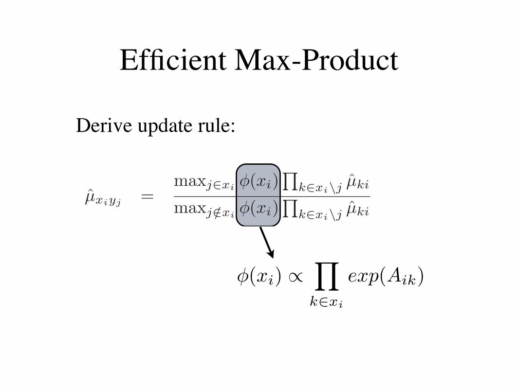
!(xi) !!
k!xi
exp(Aik)
Efficient Max-Product
Derive update rule:
mxi(yj) =1
Zmax
xi
!
"!(xi)"(xi, yj)#
k !=j
myk(xi)
$
%
b(xi) =1
Z!(xi)
#
k
myk(xi)
Loopy belief propagation on this graph converges tothe optimum. However, since there are
&
nb
'
possiblesettings for each variable, direct belief propagation isnot feasible with larger graphs.
3.2 EFFICIENT BELIEF PROPAGATIONOF
&
nb
'
-LENGTH MESSAGE VECTORS
We exploit three peculiarities of the above formulationto fully represent the
&nb
'
length messages as scalars.
First, the " functions are well structured, and theirstructure causes the maximization term in the messageupdates to always be one of two values.
mxi(yj) ! maxvj"xi
!(xi)#
k !=j
myk(xi), if ui " yj
mxi(yj) ! maxvj /"xi
!(xi)#
k !=j
myk(xi), if ui /" yj (4)
This is because the " function changes based only onwhether the setting of yj indicates that vj shares anedge with ui. Furthermore, if we redefine the abovemessage values as two scalars, we can write the mes-sages more specifically as
µxiyj ! maxvj"xi
!(xi)#
uk"xi\vj
µki
#
uk /"xi\vj
#ki
#xiyj ! maxvj /"xi
!(xi)#
uk"xi\vj
µki
#
uk /"xi\vj
#ki. (5)
Second, since the messages are unnormalized proba-bilities, we can divide any constant from the vectorswithout changing the result. We divide all entries inthe message vector by #xiyj to get
µxiyj =µxiyj
#xiyj
and #xiyj = 1 .
This lossless compression scheme simplifies the storageof message vectors from length
&
nb
'
to 1.
We rewrite the ! functions as a product of the expo-nentiated Aij weights and eliminate the need to ex-haustively maximize over all possible sets of size b. In-serting Equation (2) into the definition of µxiyj gives
µxiyj =maxj"xi !(xi)
(
k"xi\j µki
maxj /"xi!(xi)
(
k"xi\j µki
=maxj"xi
(
k"xiexp(Aik)
(
k"xi\j µki
maxj /"xi
(
k"xiexp(Aik)
(
k"xi\j µki
=exp(Aij)maxj"xi
(
k"xi\j exp(Aik)µki
maxj /"xi
(
k"xiexp(Aij)µki
(6)
We cancel out common terms and are left with thesimple message update rule,
µxiyj =exp(Aij)
exp(Ai!)µy!xi
.
Here, the index $ refers to the the bth greatest set-ting of k for the term exp(Aik)myk(xi), where k #= j.This compressed version of a message update can becomputed in O(bn) time.
We cannot e!ciently reconstruct the entire belief vec-tor but we can e!ciently find its maximum.
maxxi
b(xi) ! maxxi
!(xi)#
k"xi
µykxi
! maxxi
#
k"xi
exp(Aik)µykxi (7)
Finally, to maximize over xi we enumerate k andgreedily select the b largest values of exp(Aik)µykxi .
The above procedure avoids enumerating all&n
b
'
en-tries in the belief vector, and instead reshapes the dis-tribution into a b dimensional hypercube. The maxi-mum of the hypercube is found e!ciently by searchingeach dimension independently. Note that each dimen-sion represents one of the b edges for node ui.
4 PROOF OF CONVERGENCE
We begin with the assumption that MG, the maxi-mum weight b-matching on G, is unique. Moreover,W(MG), the weight of MG, is greater than that of anyother matching by a constant %.
% = W(MG) $ maxM !=MG
W(M)
Let T be the unwrapped graph of G from node ui. Anunwrapped graph is a tree that contains representa-tions of all paths of length d in G originating from asingle root node without any backtracking. Each nodein T maps to a corresponding node in G, and each nodein G maps to multiple nodes in T . Nodes and edges inT have the same local connectivity and potential func-tions as their corresponding nodes in G. Let r be theroot of T that corresponds to ui in the original graph
bth greatest setting of k for the term
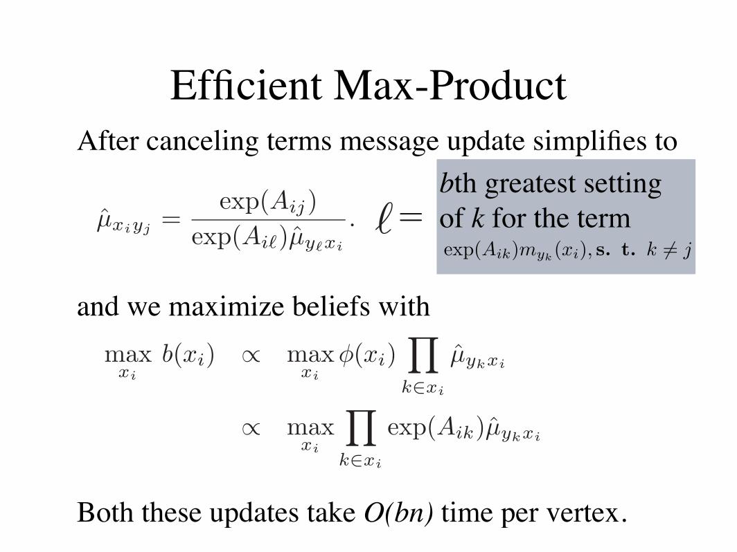
Efficient Max-ProductAfter canceling terms message update simplifies to
and we maximize beliefs with
Both these updates take O(bn) time per vertex.
mxi(yj) =1
Zmax
xi
!
"!(xi)"(xi, yj)#
k !=j
myk(xi)
$
%
b(xi) =1
Z!(xi)
#
k
myk(xi)
Loopy belief propagation on this graph converges tothe optimum. However, since there are
&
nb
'
possiblesettings for each variable, direct belief propagation isnot feasible with larger graphs.
3.2 EFFICIENT BELIEF PROPAGATIONOF
&
nb
'
-LENGTH MESSAGE VECTORS
We exploit three peculiarities of the above formulationto fully represent the
&nb
'
length messages as scalars.
First, the " functions are well structured, and theirstructure causes the maximization term in the messageupdates to always be one of two values.
mxi(yj) ! maxvj"xi
!(xi)#
k !=j
myk(xi), if ui " yj
mxi(yj) ! maxvj /"xi
!(xi)#
k !=j
myk(xi), if ui /" yj (4)
This is because the " function changes based only onwhether the setting of yj indicates that vj shares anedge with ui. Furthermore, if we redefine the abovemessage values as two scalars, we can write the mes-sages more specifically as
µxiyj ! maxvj"xi
!(xi)#
uk"xi\vj
µki
#
uk /"xi\vj
#ki
#xiyj ! maxvj /"xi
!(xi)#
uk"xi\vj
µki
#
uk /"xi\vj
#ki. (5)
Second, since the messages are unnormalized proba-bilities, we can divide any constant from the vectorswithout changing the result. We divide all entries inthe message vector by #xiyj to get
µxiyj =µxiyj
#xiyj
and #xiyj = 1 .
This lossless compression scheme simplifies the storageof message vectors from length
&
nb
'
to 1.
We rewrite the ! functions as a product of the expo-nentiated Aij weights and eliminate the need to ex-haustively maximize over all possible sets of size b. In-serting Equation (2) into the definition of µxiyj gives
µxiyj =maxj"xi !(xi)
(
k"xi\j µki
maxj /"xi!(xi)
(
k"xi\j µki
=maxj"xi
(
k"xiexp(Aik)
(
k"xi\j µki
maxj /"xi
(
k"xiexp(Aik)
(
k"xi\j µki
=exp(Aij)maxj"xi
(
k"xi\j exp(Aik)µki
maxj /"xi
(
k"xiexp(Aij)µki
(6)
We cancel out common terms and are left with thesimple message update rule,
µxiyj =exp(Aij)
exp(Ai!)µy!xi
.
Here, the index $ refers to the the bth greatest set-ting of k for the term exp(Aik)myk(xi), where k #= j.This compressed version of a message update can becomputed in O(bn) time.
We cannot e!ciently reconstruct the entire belief vec-tor but we can e!ciently find its maximum.
maxxi
b(xi) ! maxxi
!(xi)#
k"xi
µykxi
! maxxi
#
k"xi
exp(Aik)µykxi (7)
Finally, to maximize over xi we enumerate k andgreedily select the b largest values of exp(Aik)µykxi .
The above procedure avoids enumerating all&n
b
'
en-tries in the belief vector, and instead reshapes the dis-tribution into a b dimensional hypercube. The maxi-mum of the hypercube is found e!ciently by searchingeach dimension independently. Note that each dimen-sion represents one of the b edges for node ui.
4 PROOF OF CONVERGENCE
We begin with the assumption that MG, the maxi-mum weight b-matching on G, is unique. Moreover,W(MG), the weight of MG, is greater than that of anyother matching by a constant %.
% = W(MG) $ maxM !=MG
W(M)
Let T be the unwrapped graph of G from node ui. Anunwrapped graph is a tree that contains representa-tions of all paths of length d in G originating from asingle root node without any backtracking. Each nodein T maps to a corresponding node in G, and each nodein G maps to multiple nodes in T . Nodes and edges inT have the same local connectivity and potential func-tions as their corresponding nodes in G. Let r be theroot of T that corresponds to ui in the original graph
=
exp(Aik)myk(xi), s. t. k != j
1. Bipartite Weighted b-Matching
2. Edge Weights As a Distribution
3. Efficient Max-Product
4. Convergence Proof Sketch
5. Experiments
6. Discussion
Outline

Convergence Proof Sketch
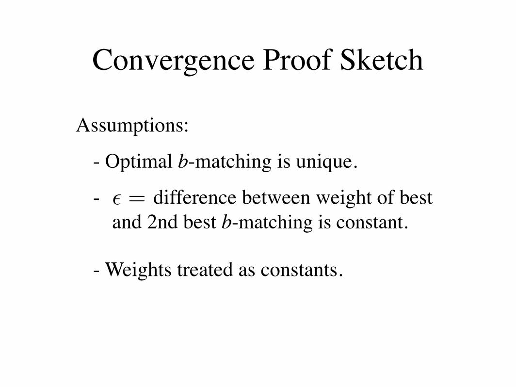
Convergence Proof Sketch
Assumptions:
- Optimal b-matching is unique.
-
- Weights treated as constants.
! = difference between weight of best and 2nd best b-matching is constant.
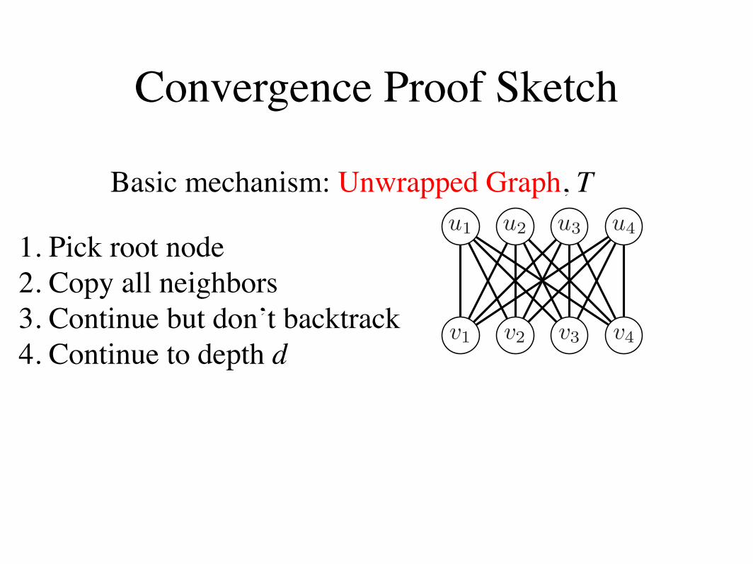
Basic mechanism: Unwrapped Graph, T
Loopy Belief Propagation for Bipartite Maximum Weight b-Matching
Bert Huang
Computer Science Dept.Columbia UniversityNew York, NY 10027
Tony Jebara
Computer Science Dept.Columbia UniversityNew York, NY 10027
Abstract
We formulate the weighted b-matching ob-jective function as a probability distributionfunction and prove that belief propagation(BP) on its graphical model converges tothe optimum. Standard BP on our graphi-cal model cannot be computed in polynomialtime, but we introduce an algebraic methodto circumvent the combinatorial message up-dates. Empirically, the resulting algorithmis on average faster than popular combina-torial implementations, while still scaling atthe same asymptotic rate of O(bn3). Further-more, the algorithm shows promising perfor-mance in machine learning applications.
1 INTRODUCTION
u1 u2 u3 u4
v1 v2 v3 v4
Figure 1: Example b-matching MG on a bipartite graph G.Dashed lines represent possible edges, solid lines representb-matched edges. In this case b = 2.
2 EXPERIMENTS
We elaborate the speed advantages of our method andan application in machine learning where b-matchingcan improve classification accuracy.
2.1 RUNNING TIME ANALYSIS
We compare the performance of our implementationof belief propagation maximum weighted b-matching
u1 u2 u3 u4
v1 v2 v3 v4
1,5 234 6
Figure 3: The cyclic alternating path PG starting at v1 onG that corresponds to the nodes visited by PT . Edges arenumbered to help follow the loopy path.
against the free graph optimization package, GOBLIN.1
Classical b-matching algorithms such as the balancednetwork flow method used by the GOBLIN library runin O(bn3) time [?]. The belief propagation methodtakes O(bn) time to compute one iteration of messageupdates for each of the 2n nodes and converges in O(n)iterations. So, its overall running time is also O(bn3).
We ran both algorithms on randomly generated bipar-tite graphs of 10 ! n ! 100 and 1 ! b ! n/2. Wegenerated the weight matrix with the rand functionin MATLAB, which picks each weight independentlyfrom a uniform distribution between 0 and 1.
The GOBLIN library is C++ code and our implemen-tation2 of belief propagation b-matching is in C. Bothwere run on a 3.00 Ghz. Pentium 4 processor.
In general, the belief propagation runs hundreds oftimes faster than GOBLIN. Figure 5 shows variouscomparisons of their running times. The surface plotsshow how the algorithms scale with respect to n andb. The line plots show cross sections of these surfaceplots, with appropriate transformations on the run-ning time to show the scaling (without these transfor-mations, the belief propagation line would appear tobe always zero due to the scale of the plot following
1Available at: http://www.math.uni-augsburg.de/opt/goblin.html2Available at http://www.cs.columbia.edu/bert/bmatching
Convergence Proof Sketch
1. Pick root node2. Copy all neighbors3. Continue but don’t backtrack4. Continue to depth d
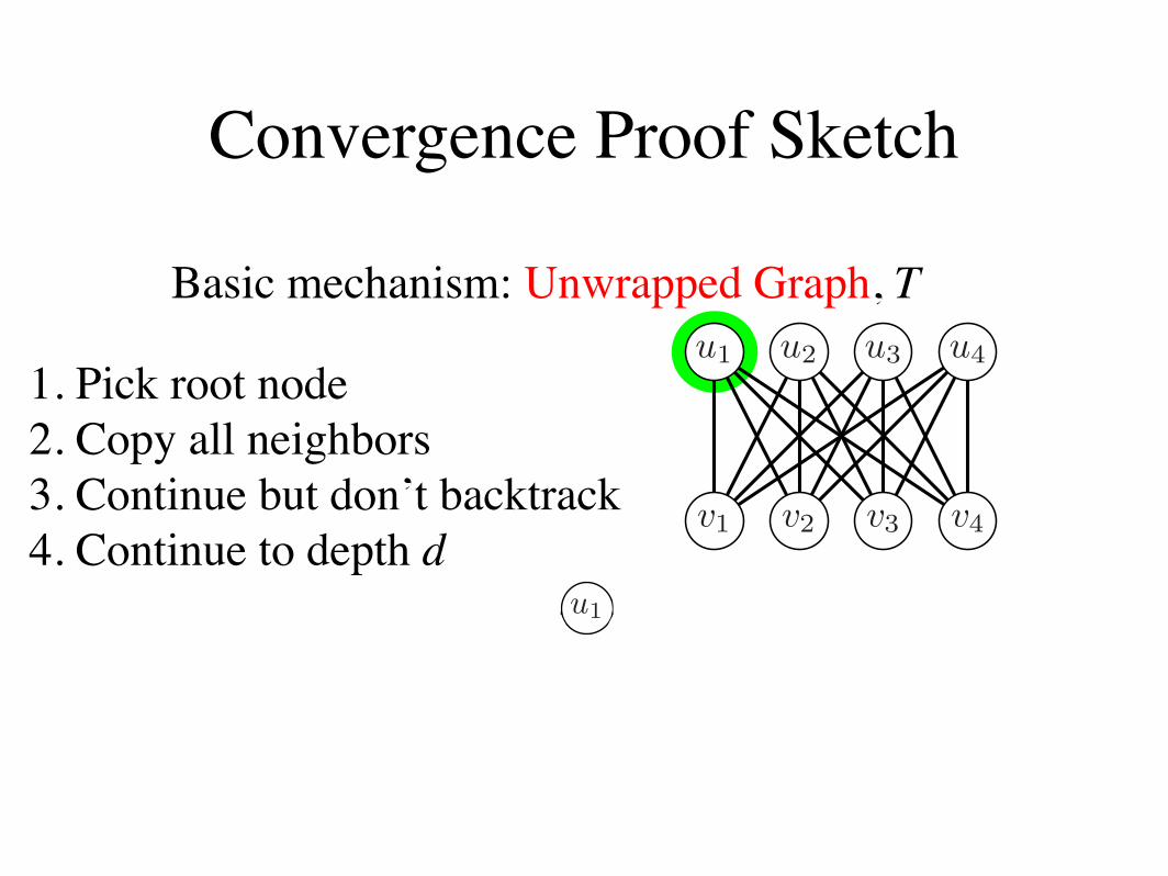
Basic mechanism: Unwrapped Graph, T
u1
v1 v2 v3 v4
u2 u2 u2 u2u3 u3 u3 u3u4 u4 u4 u4
v2 v3 v4 v2 v3 v4 v2 v3 v4 v1 v3 v4 v1 v3 v4 v1 v3 v4 v1 v2 v4 v1 v2 v4 v1 v2 v4 v1 v2 v3 v1 v2 v3 v1 v2 v3
Figure 2: Example unwrapped graph T of G at 3 iterations. The matching MT is highlighted based on MG from Figure1. Note that leaf nodes cannot have perfect b-matchings, but all inner nodes and the root do. One possible path PT ishighlighted, which is discussed in Lemma ??.
. . .u2v2u4v1u1v3u4v1u3
First cycle
(a) PG
u4
v3u1
v1
(b) c1
. . .u2v2u4v1u3
(c) PG \ c1
Figure 4: (a) One possible extension of PG from Figure 1. This path comes from a deeper T so PG is longer. The firstcycle c1 detected is highlighted. (b) Cycle c1 from PG. (c) The remainder of PG when we remove c1. Note the alternationof the matched edges remains consistent even when we cut out cycles in the interior of the path.
the GOBLIN line). Since both algorithms have run-ning time O(bn3), when we fix b = 5, we get a cubiccurve. When we fix b = n/2, we get a quartic curvebecause b becomes a function of n.
20
40
204060801000
0.1
b
BP median running time
n
t
20
40
204060801000
100
b
GOBLIN median running time
n
t
20 40 60 80 1000
1
2
3
n
t1/3
Median Running time when B=5
20 40 60 80 1000
1
2
3
4
n
t1/4
Median Running time when B=! n/2 "
GOBLIN
BP
GOBLIN
BP
Figure 5: Median running time in seconds on randomlyweighted graphs for the GOBLIN library and BP. Top Left:BP median running time with respect to n, b. Bottom Left:GOBLIN b-matching solver median running time over n,b. Top Right: Cube root of running time ( 3
!t) of both
algorithms when b = 3; note that both scale linearly inthis plot, implying a n3 term in running time for both.Bottom Right: Root-4 ( 4
!t) of running time for various n,
when b = "n/2#. Both algorithms have quartic runningtime.
2.2 b-MATCHING FOR CLASSIFICATION
One natural application of b-matching is as an im-provement over k-nearest neighbor (KNN) for classi-fication. Using KNN for classification is a quick wayof computing a reasonable prediction of class, but it isinherently greedy. The algorithm starts by computingan a!nity matrix between all data points. For eachtest data point, KNN greedily selects its k neighborsregardless of the connectivity or graph this may gener-ate. This invariably leads to some nodes serving as hubnodes and labeling too many unknown examples whileother training points are never used as neighbors.
Instead, using b-matching enforces uniform connectiv-ity across the training and testing points. For exam-ple, assume the number of testing points and trainingpoints is the same and we perform b-matching. Then,each testing point will be labeled by b training pointsand each training point contributes to the labeling ofb testing points. This means b-matching will do a bet-ter job of recreating the distribution of classes seenin the training data when it classifies test data. Thisis useful when test data is transformed in some waythat preserves the shape of the distribution, but it istranslated or scaled to confuse KNN. This can occur insituations where training data comes from a di"erentsource than the testing data.
In both algorithms, we compute a bipartite a!nitygraph between a set of training points and a set oftesting points. We fix the cardinalities of these setsto be equal (though if they are unequal we can down-sample and run the algorithm in multiple folds to ob-
Loopy Belief Propagation for Bipartite Maximum Weight b-Matching
Bert Huang
Computer Science Dept.Columbia UniversityNew York, NY 10027
Tony Jebara
Computer Science Dept.Columbia UniversityNew York, NY 10027
Abstract
We formulate the weighted b-matching ob-jective function as a probability distributionfunction and prove that belief propagation(BP) on its graphical model converges tothe optimum. Standard BP on our graphi-cal model cannot be computed in polynomialtime, but we introduce an algebraic methodto circumvent the combinatorial message up-dates. Empirically, the resulting algorithmis on average faster than popular combina-torial implementations, while still scaling atthe same asymptotic rate of O(bn3). Further-more, the algorithm shows promising perfor-mance in machine learning applications.
1 INTRODUCTION
u1 u2 u3 u4
v1 v2 v3 v4
Figure 1: Example b-matching MG on a bipartite graph G.Dashed lines represent possible edges, solid lines representb-matched edges. In this case b = 2.
2 EXPERIMENTS
We elaborate the speed advantages of our method andan application in machine learning where b-matchingcan improve classification accuracy.
2.1 RUNNING TIME ANALYSIS
We compare the performance of our implementationof belief propagation maximum weighted b-matching
u1 u2 u3 u4
v1 v2 v3 v4
1,5 234 6
Figure 3: The cyclic alternating path PG starting at v1 onG that corresponds to the nodes visited by PT . Edges arenumbered to help follow the loopy path.
against the free graph optimization package, GOBLIN.1
Classical b-matching algorithms such as the balancednetwork flow method used by the GOBLIN library runin O(bn3) time [?]. The belief propagation methodtakes O(bn) time to compute one iteration of messageupdates for each of the 2n nodes and converges in O(n)iterations. So, its overall running time is also O(bn3).
We ran both algorithms on randomly generated bipar-tite graphs of 10 ! n ! 100 and 1 ! b ! n/2. Wegenerated the weight matrix with the rand functionin MATLAB, which picks each weight independentlyfrom a uniform distribution between 0 and 1.
The GOBLIN library is C++ code and our implemen-tation2 of belief propagation b-matching is in C. Bothwere run on a 3.00 Ghz. Pentium 4 processor.
In general, the belief propagation runs hundreds oftimes faster than GOBLIN. Figure 5 shows variouscomparisons of their running times. The surface plotsshow how the algorithms scale with respect to n andb. The line plots show cross sections of these surfaceplots, with appropriate transformations on the run-ning time to show the scaling (without these transfor-mations, the belief propagation line would appear tobe always zero due to the scale of the plot following
1Available at: http://www.math.uni-augsburg.de/opt/goblin.html2Available at http://www.cs.columbia.edu/bert/bmatching
Convergence Proof Sketch
1. Pick root node2. Copy all neighbors3. Continue but don’t backtrack4. Continue to depth d
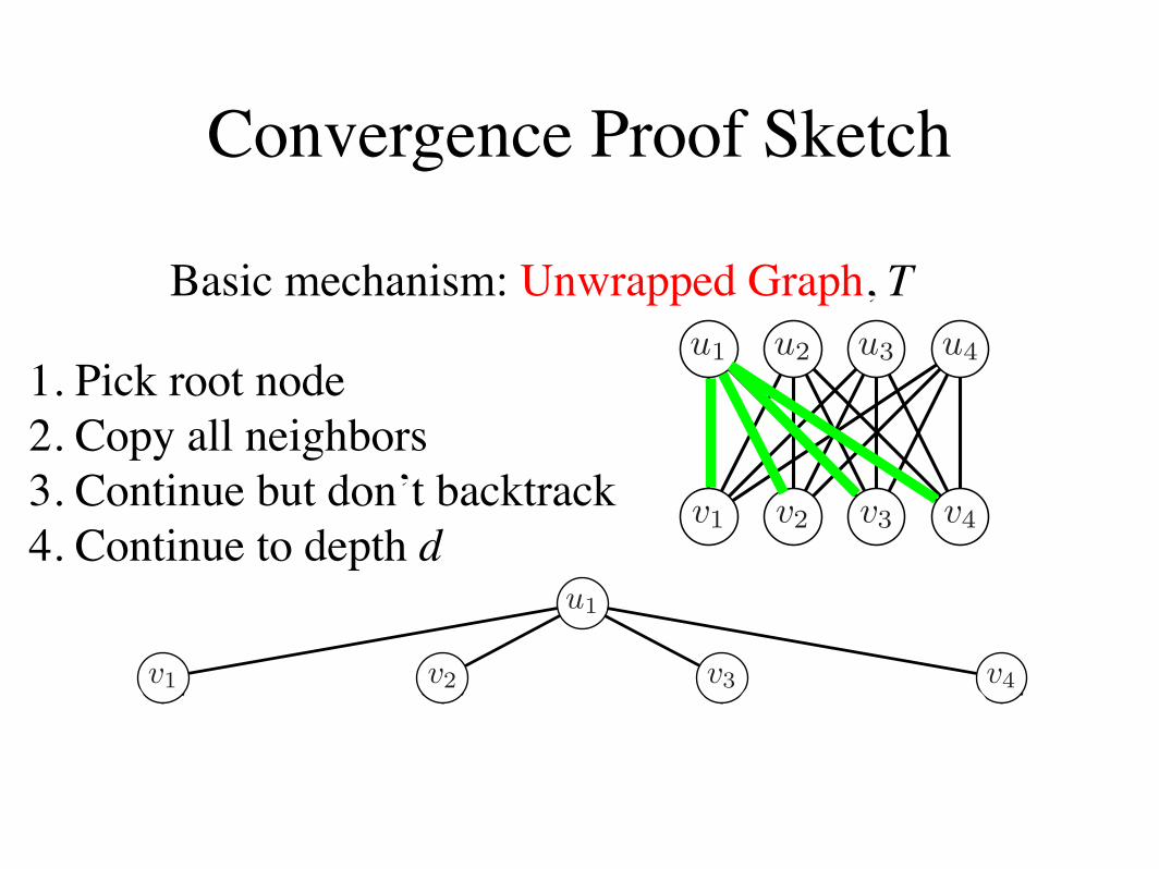
Convergence Proof Sketch
Basic mechanism: Unwrapped Graph, T
Loopy Belief Propagation for Bipartite Maximum Weight b-Matching
Bert Huang
Computer Science Dept.Columbia UniversityNew York, NY 10027
Tony Jebara
Computer Science Dept.Columbia UniversityNew York, NY 10027
Abstract
We formulate the weighted b-matching ob-jective function as a probability distributionfunction and prove that belief propagation(BP) on its graphical model converges tothe optimum. Standard BP on our graphi-cal model cannot be computed in polynomialtime, but we introduce an algebraic methodto circumvent the combinatorial message up-dates. Empirically, the resulting algorithmis on average faster than popular combina-torial implementations, while still scaling atthe same asymptotic rate of O(bn3). Further-more, the algorithm shows promising perfor-mance in machine learning applications.
1 INTRODUCTION
u1 u2 u3 u4
v1 v2 v3 v4
Figure 1: Example b-matching MG on a bipartite graph G.Dashed lines represent possible edges, solid lines representb-matched edges. In this case b = 2.
2 EXPERIMENTS
We elaborate the speed advantages of our method andan application in machine learning where b-matchingcan improve classification accuracy.
2.1 RUNNING TIME ANALYSIS
We compare the performance of our implementationof belief propagation maximum weighted b-matching
u1 u2 u3 u4
v1 v2 v3 v4
1,5 234 6
Figure 3: The cyclic alternating path PG starting at v1 onG that corresponds to the nodes visited by PT . Edges arenumbered to help follow the loopy path.
against the free graph optimization package, GOBLIN.1
Classical b-matching algorithms such as the balancednetwork flow method used by the GOBLIN library runin O(bn3) time [?]. The belief propagation methodtakes O(bn) time to compute one iteration of messageupdates for each of the 2n nodes and converges in O(n)iterations. So, its overall running time is also O(bn3).
We ran both algorithms on randomly generated bipar-tite graphs of 10 ! n ! 100 and 1 ! b ! n/2. Wegenerated the weight matrix with the rand functionin MATLAB, which picks each weight independentlyfrom a uniform distribution between 0 and 1.
The GOBLIN library is C++ code and our implemen-tation2 of belief propagation b-matching is in C. Bothwere run on a 3.00 Ghz. Pentium 4 processor.
In general, the belief propagation runs hundreds oftimes faster than GOBLIN. Figure 5 shows variouscomparisons of their running times. The surface plotsshow how the algorithms scale with respect to n andb. The line plots show cross sections of these surfaceplots, with appropriate transformations on the run-ning time to show the scaling (without these transfor-mations, the belief propagation line would appear tobe always zero due to the scale of the plot following
1Available at: http://www.math.uni-augsburg.de/opt/goblin.html2Available at http://www.cs.columbia.edu/bert/bmatching
u1
v1 v2 v3 v4
u2 u2 u2 u2u3 u3 u3 u3u4 u4 u4 u4
v2 v3 v4 v2 v3 v4 v2 v3 v4 v1 v3 v4 v1 v3 v4 v1 v3 v4 v1 v2 v4 v1 v2 v4 v1 v2 v4 v1 v2 v3 v1 v2 v3 v1 v2 v3
Figure 2: Example unwrapped graph T of G at 3 iterations. The matching MT is highlighted based on MG from Figure1. Note that leaf nodes cannot have perfect b-matchings, but all inner nodes and the root do. One possible path PT ishighlighted, which is discussed in Lemma ??.
. . .u2v2u4v1u1v3u4v1u3
First cycle
(a) PG
u4
v3u1
v1
(b) c1
. . .u2v2u4v1u3
(c) PG \ c1
Figure 4: (a) One possible extension of PG from Figure 1. This path comes from a deeper T so PG is longer. The firstcycle c1 detected is highlighted. (b) Cycle c1 from PG. (c) The remainder of PG when we remove c1. Note the alternationof the matched edges remains consistent even when we cut out cycles in the interior of the path.
the GOBLIN line). Since both algorithms have run-ning time O(bn3), when we fix b = 5, we get a cubiccurve. When we fix b = n/2, we get a quartic curvebecause b becomes a function of n.
20
40
204060801000
0.1
b
BP median running time
n
t
20
40
204060801000
100
b
GOBLIN median running time
n
t
20 40 60 80 1000
1
2
3
n
t1/3
Median Running time when B=5
20 40 60 80 1000
1
2
3
4
n
t1/4
Median Running time when B=! n/2 "
GOBLIN
BP
GOBLIN
BP
Figure 5: Median running time in seconds on randomlyweighted graphs for the GOBLIN library and BP. Top Left:BP median running time with respect to n, b. Bottom Left:GOBLIN b-matching solver median running time over n,b. Top Right: Cube root of running time ( 3
!t) of both
algorithms when b = 3; note that both scale linearly inthis plot, implying a n3 term in running time for both.Bottom Right: Root-4 ( 4
!t) of running time for various n,
when b = "n/2#. Both algorithms have quartic runningtime.
2.2 b-MATCHING FOR CLASSIFICATION
One natural application of b-matching is as an im-provement over k-nearest neighbor (KNN) for classi-fication. Using KNN for classification is a quick wayof computing a reasonable prediction of class, but it isinherently greedy. The algorithm starts by computingan a!nity matrix between all data points. For eachtest data point, KNN greedily selects its k neighborsregardless of the connectivity or graph this may gener-ate. This invariably leads to some nodes serving as hubnodes and labeling too many unknown examples whileother training points are never used as neighbors.
Instead, using b-matching enforces uniform connectiv-ity across the training and testing points. For exam-ple, assume the number of testing points and trainingpoints is the same and we perform b-matching. Then,each testing point will be labeled by b training pointsand each training point contributes to the labeling ofb testing points. This means b-matching will do a bet-ter job of recreating the distribution of classes seenin the training data when it classifies test data. Thisis useful when test data is transformed in some waythat preserves the shape of the distribution, but it istranslated or scaled to confuse KNN. This can occur insituations where training data comes from a di"erentsource than the testing data.
In both algorithms, we compute a bipartite a!nitygraph between a set of training points and a set oftesting points. We fix the cardinalities of these setsto be equal (though if they are unequal we can down-sample and run the algorithm in multiple folds to ob-
1. Pick root node2. Copy all neighbors3. Continue but don’t backtrack4. Continue to depth d
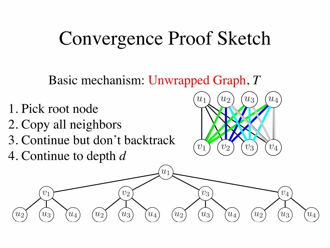
Convergence Proof Sketch
Basic mechanism: Unwrapped Graph, T
Loopy Belief Propagation for Bipartite Maximum Weight b-Matching
Bert Huang
Computer Science Dept.Columbia UniversityNew York, NY 10027
Tony Jebara
Computer Science Dept.Columbia UniversityNew York, NY 10027
Abstract
We formulate the weighted b-matching ob-jective function as a probability distributionfunction and prove that belief propagation(BP) on its graphical model converges tothe optimum. Standard BP on our graphi-cal model cannot be computed in polynomialtime, but we introduce an algebraic methodto circumvent the combinatorial message up-dates. Empirically, the resulting algorithmis on average faster than popular combina-torial implementations, while still scaling atthe same asymptotic rate of O(bn3). Further-more, the algorithm shows promising perfor-mance in machine learning applications.
1 INTRODUCTION
u1 u2 u3 u4
v1 v2 v3 v4
Figure 1: Example b-matching MG on a bipartite graph G.Dashed lines represent possible edges, solid lines representb-matched edges. In this case b = 2.
2 EXPERIMENTS
We elaborate the speed advantages of our method andan application in machine learning where b-matchingcan improve classification accuracy.
2.1 RUNNING TIME ANALYSIS
We compare the performance of our implementationof belief propagation maximum weighted b-matching
u1 u2 u3 u4
v1 v2 v3 v4
1,5 234 6
Figure 3: The cyclic alternating path PG starting at v1 onG that corresponds to the nodes visited by PT . Edges arenumbered to help follow the loopy path.
against the free graph optimization package, GOBLIN.1
Classical b-matching algorithms such as the balancednetwork flow method used by the GOBLIN library runin O(bn3) time [?]. The belief propagation methodtakes O(bn) time to compute one iteration of messageupdates for each of the 2n nodes and converges in O(n)iterations. So, its overall running time is also O(bn3).
We ran both algorithms on randomly generated bipar-tite graphs of 10 ! n ! 100 and 1 ! b ! n/2. Wegenerated the weight matrix with the rand functionin MATLAB, which picks each weight independentlyfrom a uniform distribution between 0 and 1.
The GOBLIN library is C++ code and our implemen-tation2 of belief propagation b-matching is in C. Bothwere run on a 3.00 Ghz. Pentium 4 processor.
In general, the belief propagation runs hundreds oftimes faster than GOBLIN. Figure 5 shows variouscomparisons of their running times. The surface plotsshow how the algorithms scale with respect to n andb. The line plots show cross sections of these surfaceplots, with appropriate transformations on the run-ning time to show the scaling (without these transfor-mations, the belief propagation line would appear tobe always zero due to the scale of the plot following
1Available at: http://www.math.uni-augsburg.de/opt/goblin.html2Available at http://www.cs.columbia.edu/bert/bmatching
u1
v1 v2 v3 v4
u2 u2 u2 u2u3 u3 u3 u3u4 u4 u4 u4
v2 v3 v4 v2 v3 v4 v2 v3 v4 v1 v3 v4 v1 v3 v4 v1 v3 v4 v1 v2 v4 v1 v2 v4 v1 v2 v4 v1 v2 v3 v1 v2 v3 v1 v2 v3
Figure 2: Example unwrapped graph T of G at 3 iterations. The matching MT is highlighted based on MG from Figure1. Note that leaf nodes cannot have perfect b-matchings, but all inner nodes and the root do. One possible path PT ishighlighted, which is discussed in Lemma ??.
. . .u2v2u4v1u1v3u4v1u3
First cycle
(a) PG
u4
v3u1
v1
(b) c1
. . .u2v2u4v1u3
(c) PG \ c1
Figure 4: (a) One possible extension of PG from Figure 1. This path comes from a deeper T so PG is longer. The firstcycle c1 detected is highlighted. (b) Cycle c1 from PG. (c) The remainder of PG when we remove c1. Note the alternationof the matched edges remains consistent even when we cut out cycles in the interior of the path.
the GOBLIN line). Since both algorithms have run-ning time O(bn3), when we fix b = 5, we get a cubiccurve. When we fix b = n/2, we get a quartic curvebecause b becomes a function of n.
20
40
204060801000
0.1
b
BP median running time
n
t
20
40
204060801000
100
b
GOBLIN median running time
n
t
20 40 60 80 1000
1
2
3
n
t1/3
Median Running time when B=5
20 40 60 80 1000
1
2
3
4
n
t1/4
Median Running time when B=! n/2 "
GOBLIN
BP
GOBLIN
BP
Figure 5: Median running time in seconds on randomlyweighted graphs for the GOBLIN library and BP. Top Left:BP median running time with respect to n, b. Bottom Left:GOBLIN b-matching solver median running time over n,b. Top Right: Cube root of running time ( 3
!t) of both
algorithms when b = 3; note that both scale linearly inthis plot, implying a n3 term in running time for both.Bottom Right: Root-4 ( 4
!t) of running time for various n,
when b = "n/2#. Both algorithms have quartic runningtime.
2.2 b-MATCHING FOR CLASSIFICATION
One natural application of b-matching is as an im-provement over k-nearest neighbor (KNN) for classi-fication. Using KNN for classification is a quick wayof computing a reasonable prediction of class, but it isinherently greedy. The algorithm starts by computingan a!nity matrix between all data points. For eachtest data point, KNN greedily selects its k neighborsregardless of the connectivity or graph this may gener-ate. This invariably leads to some nodes serving as hubnodes and labeling too many unknown examples whileother training points are never used as neighbors.
Instead, using b-matching enforces uniform connectiv-ity across the training and testing points. For exam-ple, assume the number of testing points and trainingpoints is the same and we perform b-matching. Then,each testing point will be labeled by b training pointsand each training point contributes to the labeling ofb testing points. This means b-matching will do a bet-ter job of recreating the distribution of classes seenin the training data when it classifies test data. Thisis useful when test data is transformed in some waythat preserves the shape of the distribution, but it istranslated or scaled to confuse KNN. This can occur insituations where training data comes from a di"erentsource than the testing data.
In both algorithms, we compute a bipartite a!nitygraph between a set of training points and a set oftesting points. We fix the cardinalities of these setsto be equal (though if they are unequal we can down-sample and run the algorithm in multiple folds to ob-
1. Pick root node2. Copy all neighbors3. Continue but don’t backtrack4. Continue to depth d
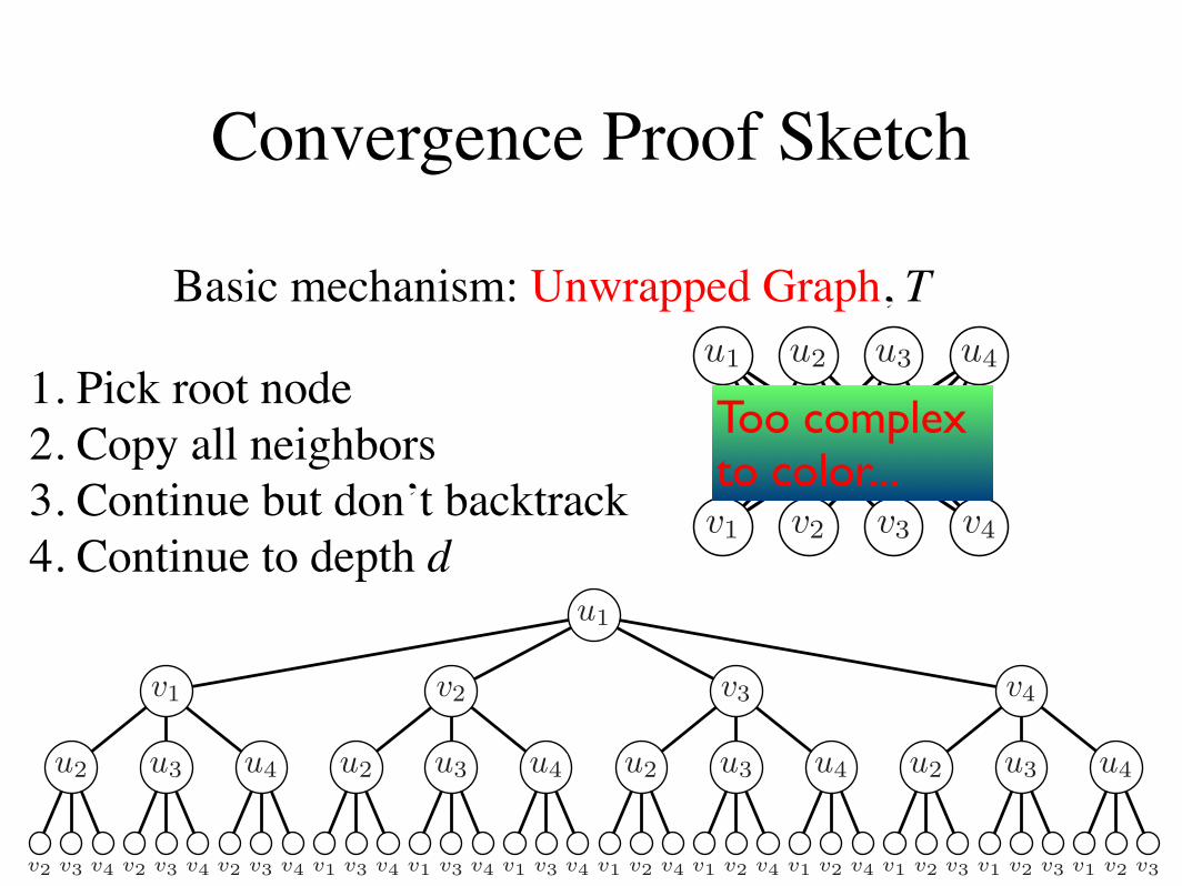
Convergence Proof Sketch
Basic mechanism: Unwrapped Graph, T
Loopy Belief Propagation for Bipartite Maximum Weight b-Matching
Bert Huang
Computer Science Dept.Columbia UniversityNew York, NY 10027
Tony Jebara
Computer Science Dept.Columbia UniversityNew York, NY 10027
Abstract
We formulate the weighted b-matching ob-jective function as a probability distributionfunction and prove that belief propagation(BP) on its graphical model converges tothe optimum. Standard BP on our graphi-cal model cannot be computed in polynomialtime, but we introduce an algebraic methodto circumvent the combinatorial message up-dates. Empirically, the resulting algorithmis on average faster than popular combina-torial implementations, while still scaling atthe same asymptotic rate of O(bn3). Further-more, the algorithm shows promising perfor-mance in machine learning applications.
1 INTRODUCTION
u1 u2 u3 u4
v1 v2 v3 v4
Figure 1: Example b-matching MG on a bipartite graph G.Dashed lines represent possible edges, solid lines representb-matched edges. In this case b = 2.
2 EXPERIMENTS
We elaborate the speed advantages of our method andan application in machine learning where b-matchingcan improve classification accuracy.
2.1 RUNNING TIME ANALYSIS
We compare the performance of our implementationof belief propagation maximum weighted b-matching
u1 u2 u3 u4
v1 v2 v3 v4
1,5 234 6
Figure 3: The cyclic alternating path PG starting at v1 onG that corresponds to the nodes visited by PT . Edges arenumbered to help follow the loopy path.
against the free graph optimization package, GOBLIN.1
Classical b-matching algorithms such as the balancednetwork flow method used by the GOBLIN library runin O(bn3) time [?]. The belief propagation methodtakes O(bn) time to compute one iteration of messageupdates for each of the 2n nodes and converges in O(n)iterations. So, its overall running time is also O(bn3).
We ran both algorithms on randomly generated bipar-tite graphs of 10 ! n ! 100 and 1 ! b ! n/2. Wegenerated the weight matrix with the rand functionin MATLAB, which picks each weight independentlyfrom a uniform distribution between 0 and 1.
The GOBLIN library is C++ code and our implemen-tation2 of belief propagation b-matching is in C. Bothwere run on a 3.00 Ghz. Pentium 4 processor.
In general, the belief propagation runs hundreds oftimes faster than GOBLIN. Figure 5 shows variouscomparisons of their running times. The surface plotsshow how the algorithms scale with respect to n andb. The line plots show cross sections of these surfaceplots, with appropriate transformations on the run-ning time to show the scaling (without these transfor-mations, the belief propagation line would appear tobe always zero due to the scale of the plot following
1Available at: http://www.math.uni-augsburg.de/opt/goblin.html2Available at http://www.cs.columbia.edu/bert/bmatching
u1
v1 v2 v3 v4
u2 u2 u2 u2u3 u3 u3 u3u4 u4 u4 u4
v2 v3 v4 v2 v3 v4 v2 v3 v4 v1 v3 v4 v1 v3 v4 v1 v3 v4 v1 v2 v4 v1 v2 v4 v1 v2 v4 v1 v2 v3 v1 v2 v3 v1 v2 v3
Figure 2: Example unwrapped graph T of G at 3 iterations. The matching MT is highlighted based on MG from Figure1. Note that leaf nodes cannot have perfect b-matchings, but all inner nodes and the root do. One possible path PT ishighlighted, which is discussed in Lemma ??.
. . .u2v2u4v1u1v3u4v1u3
First cycle
(a) PG
u4
v3u1
v1
(b) c1
. . .u2v2u4v1u3
(c) PG \ c1
Figure 4: (a) One possible extension of PG from Figure 1. This path comes from a deeper T so PG is longer. The firstcycle c1 detected is highlighted. (b) Cycle c1 from PG. (c) The remainder of PG when we remove c1. Note the alternationof the matched edges remains consistent even when we cut out cycles in the interior of the path.
the GOBLIN line). Since both algorithms have run-ning time O(bn3), when we fix b = 5, we get a cubiccurve. When we fix b = n/2, we get a quartic curvebecause b becomes a function of n.
20
40
204060801000
0.1
b
BP median running time
n
t
20
40
204060801000
100
b
GOBLIN median running time
n
t
20 40 60 80 1000
1
2
3
n
t1/3
Median Running time when B=5
20 40 60 80 1000
1
2
3
4
n
t1/4
Median Running time when B=! n/2 "
GOBLIN
BP
GOBLIN
BP
Figure 5: Median running time in seconds on randomlyweighted graphs for the GOBLIN library and BP. Top Left:BP median running time with respect to n, b. Bottom Left:GOBLIN b-matching solver median running time over n,b. Top Right: Cube root of running time ( 3
!t) of both
algorithms when b = 3; note that both scale linearly inthis plot, implying a n3 term in running time for both.Bottom Right: Root-4 ( 4
!t) of running time for various n,
when b = "n/2#. Both algorithms have quartic runningtime.
2.2 b-MATCHING FOR CLASSIFICATION
One natural application of b-matching is as an im-provement over k-nearest neighbor (KNN) for classi-fication. Using KNN for classification is a quick wayof computing a reasonable prediction of class, but it isinherently greedy. The algorithm starts by computingan a!nity matrix between all data points. For eachtest data point, KNN greedily selects its k neighborsregardless of the connectivity or graph this may gener-ate. This invariably leads to some nodes serving as hubnodes and labeling too many unknown examples whileother training points are never used as neighbors.
Instead, using b-matching enforces uniform connectiv-ity across the training and testing points. For exam-ple, assume the number of testing points and trainingpoints is the same and we perform b-matching. Then,each testing point will be labeled by b training pointsand each training point contributes to the labeling ofb testing points. This means b-matching will do a bet-ter job of recreating the distribution of classes seenin the training data when it classifies test data. Thisis useful when test data is transformed in some waythat preserves the shape of the distribution, but it istranslated or scaled to confuse KNN. This can occur insituations where training data comes from a di"erentsource than the testing data.
In both algorithms, we compute a bipartite a!nitygraph between a set of training points and a set oftesting points. We fix the cardinalities of these setsto be equal (though if they are unequal we can down-sample and run the algorithm in multiple folds to ob-
Too complex to color...
1. Pick root node2. Copy all neighbors3. Continue but don’t backtrack4. Continue to depth d
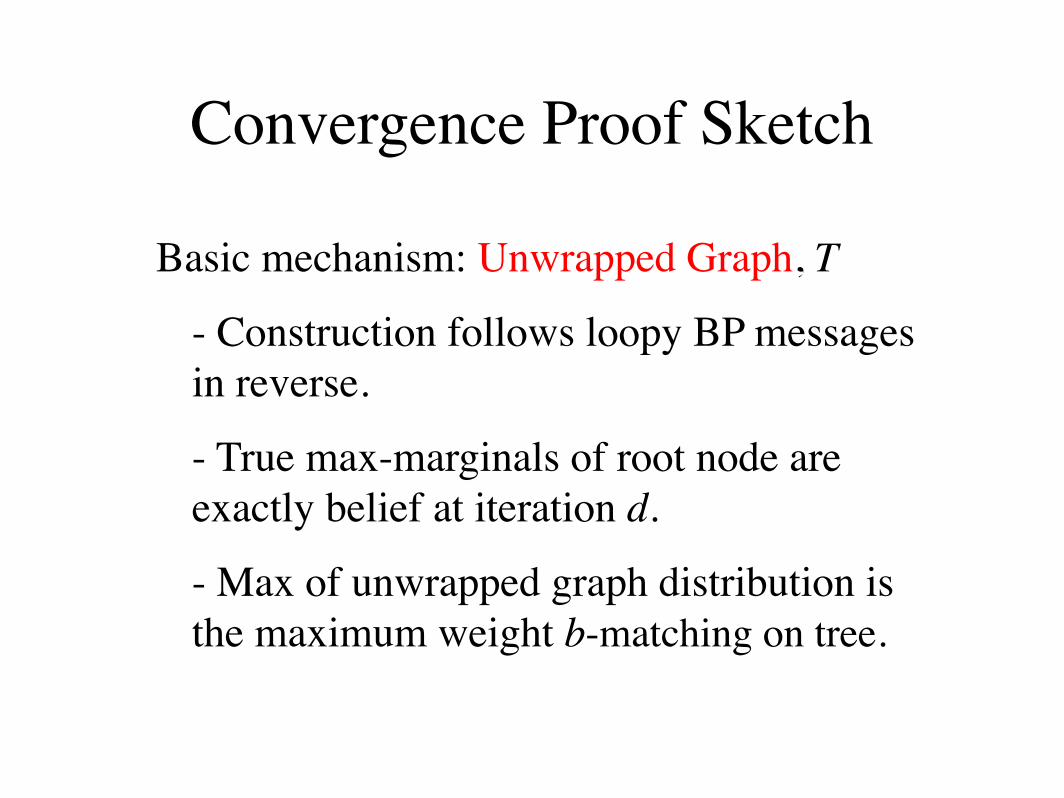
Basic mechanism: Unwrapped Graph, T
- Construction follows loopy BP messages in reverse.
- True max-marginals of root node are exactly belief at iteration d.
- Max of unwrapped graph distribution is the maximum weight b-matching on tree.
Convergence Proof Sketch
Proof by contradiction:
What happens if optimal b-matching on T differs from optimal b-matching on G at root?
Convergence Proof Sketch

Convergence Proof Sketch
u1
v1 v2 v3 v4
u2 u2 u2 u2u3 u3 u3 u3u4 u4 u4 u4
v2 v3 v4 v2 v3 v4 v2 v3 v4 v1 v3 v4 v1 v3 v4 v1 v3 v4 v1 v2 v4 v1 v2 v4 v1 v2 v4 v1 v2 v3 v1 v2 v3 v1 v2 v3
Figure 2: Example unwrapped graph T of G at 3 iterations. The matching MT is highlighted based on MG from Figure1. Note that leaf nodes cannot have perfect b-matchings, but all inner nodes and the root do. One possible path PT ishighlighted, which is discussed in Lemma ??.
. . .u2v2u4v1u1v3u4v1u3
First cycle
(a) PG
u4
v3u1
v1
(b) c1
. . .u2v2u4v1u3
(c) PG \ c1
Figure 4: (a) One possible extension of PG from Figure 1. This path comes from a deeper T so PG is longer. The firstcycle c1 detected is highlighted. (b) Cycle c1 from PG. (c) The remainder of PG when we remove c1. Note the alternationof the matched edges remains consistent even when we cut out cycles in the interior of the path.
the GOBLIN line). Since both algorithms have run-ning time O(bn3), when we fix b = 5, we get a cubiccurve. When we fix b = n/2, we get a quartic curvebecause b becomes a function of n.
20
40
204060801000
0.1
b
BP median running time
n
t
20
40
204060801000
100
b
GOBLIN median running time
n
t
20 40 60 80 1000
1
2
3
n
t1/3
Median Running time when B=5
20 40 60 80 1000
1
2
3
4
n
t1/4
Median Running time when B=! n/2 "
GOBLIN
BP
GOBLIN
BP
Figure 5: Median running time in seconds on randomlyweighted graphs for the GOBLIN library and BP. Top Left:BP median running time with respect to n, b. Bottom Left:GOBLIN b-matching solver median running time over n,b. Top Right: Cube root of running time ( 3
!t) of both
algorithms when b = 3; note that both scale linearly inthis plot, implying a n3 term in running time for both.Bottom Right: Root-4 ( 4
!t) of running time for various n,
when b = "n/2#. Both algorithms have quartic runningtime.
2.2 b-MATCHING FOR CLASSIFICATION
One natural application of b-matching is as an im-provement over k-nearest neighbor (KNN) for classi-fication. Using KNN for classification is a quick wayof computing a reasonable prediction of class, but it isinherently greedy. The algorithm starts by computingan a!nity matrix between all data points. For eachtest data point, KNN greedily selects its k neighborsregardless of the connectivity or graph this may gener-ate. This invariably leads to some nodes serving as hubnodes and labeling too many unknown examples whileother training points are never used as neighbors.
Instead, using b-matching enforces uniform connectiv-ity across the training and testing points. For exam-ple, assume the number of testing points and trainingpoints is the same and we perform b-matching. Then,each testing point will be labeled by b training pointsand each training point contributes to the labeling ofb testing points. This means b-matching will do a bet-ter job of recreating the distribution of classes seenin the training data when it classifies test data. Thisis useful when test data is transformed in some waythat preserves the shape of the distribution, but it istranslated or scaled to confuse KNN. This can occur insituations where training data comes from a di"erentsource than the testing data.
In both algorithms, we compute a bipartite a!nitygraph between a set of training points and a set oftesting points. We fix the cardinalities of these setsto be equal (though if they are unequal we can down-sample and run the algorithm in multiple folds to ob-
Best b-matching on T
Best b-matching on G copied onto T
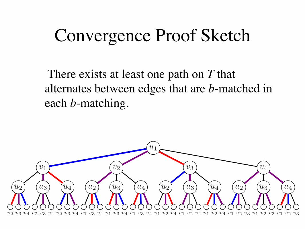
u1
v1 v2 v3 v4
u2 u2 u2 u2u3 u3 u3 u3u4 u4 u4 u4
v2 v3 v4 v2 v3 v4 v2 v3 v4 v1 v3 v4 v1 v3 v4 v1 v3 v4 v1 v2 v4 v1 v2 v4 v1 v2 v4 v1 v2 v3 v1 v2 v3 v1 v2 v3
Figure 2: Example unwrapped graph T of G at 3 iterations. The matching MT is highlighted based on MG from Figure1. Note that leaf nodes cannot have perfect b-matchings, but all inner nodes and the root do. One possible path PT ishighlighted, which is discussed in Lemma ??.
. . .u2v2u4v1u1v3u4v1u3
First cycle
(a) PG
u4
v3u1
v1
(b) c1
. . .u2v2u4v1u3
(c) PG \ c1
Figure 4: (a) One possible extension of PG from Figure 1. This path comes from a deeper T so PG is longer. The firstcycle c1 detected is highlighted. (b) Cycle c1 from PG. (c) The remainder of PG when we remove c1. Note the alternationof the matched edges remains consistent even when we cut out cycles in the interior of the path.
the GOBLIN line). Since both algorithms have run-ning time O(bn3), when we fix b = 5, we get a cubiccurve. When we fix b = n/2, we get a quartic curvebecause b becomes a function of n.
20
40
204060801000
0.1
b
BP median running time
n
t
20
40
204060801000
100
b
GOBLIN median running time
n
t
20 40 60 80 1000
1
2
3
n
t1/3
Median Running time when B=5
20 40 60 80 1000
1
2
3
4
n
t1/4
Median Running time when B=! n/2 "
GOBLIN
BP
GOBLIN
BP
Figure 5: Median running time in seconds on randomlyweighted graphs for the GOBLIN library and BP. Top Left:BP median running time with respect to n, b. Bottom Left:GOBLIN b-matching solver median running time over n,b. Top Right: Cube root of running time ( 3
!t) of both
algorithms when b = 3; note that both scale linearly inthis plot, implying a n3 term in running time for both.Bottom Right: Root-4 ( 4
!t) of running time for various n,
when b = "n/2#. Both algorithms have quartic runningtime.
2.2 b-MATCHING FOR CLASSIFICATION
One natural application of b-matching is as an im-provement over k-nearest neighbor (KNN) for classi-fication. Using KNN for classification is a quick wayof computing a reasonable prediction of class, but it isinherently greedy. The algorithm starts by computingan a!nity matrix between all data points. For eachtest data point, KNN greedily selects its k neighborsregardless of the connectivity or graph this may gener-ate. This invariably leads to some nodes serving as hubnodes and labeling too many unknown examples whileother training points are never used as neighbors.
Instead, using b-matching enforces uniform connectiv-ity across the training and testing points. For exam-ple, assume the number of testing points and trainingpoints is the same and we perform b-matching. Then,each testing point will be labeled by b training pointsand each training point contributes to the labeling ofb testing points. This means b-matching will do a bet-ter job of recreating the distribution of classes seenin the training data when it classifies test data. Thisis useful when test data is transformed in some waythat preserves the shape of the distribution, but it istranslated or scaled to confuse KNN. This can occur insituations where training data comes from a di"erentsource than the testing data.
In both algorithms, we compute a bipartite a!nitygraph between a set of training points and a set oftesting points. We fix the cardinalities of these setsto be equal (though if they are unequal we can down-sample and run the algorithm in multiple folds to ob-
There exists at least one path on T that alternates between edges that are b-matched in each b-matching.
Convergence Proof Sketch
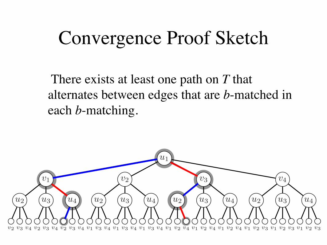
There exists at least one path on T that alternates between edges that are b-matched in each b-matching.
u1
v1 v2 v3 v4
u2 u2 u2 u2u3 u3 u3 u3u4 u4 u4 u4
v2 v3 v4 v2 v3 v4 v2 v3 v4 v1 v3 v4 v1 v3 v4 v1 v3 v4 v1 v2 v4 v1 v2 v4 v1 v2 v4 v1 v2 v3 v1 v2 v3 v1 v2 v3
Figure 2: Example unwrapped graph T of G at 3 iterations. The matching MT is highlighted based on MG from Figure1. Note that leaf nodes cannot have perfect b-matchings, but all inner nodes and the root do. One possible path PT ishighlighted, which is discussed in Lemma ??.
. . .u2v2u4v1u1v3u4v1u3
First cycle
(a) PG
u4
v3u1
v1
(b) c1
. . .u2v2u4v1u3
(c) PG \ c1
Figure 4: (a) One possible extension of PG from Figure 1. This path comes from a deeper T so PG is longer. The firstcycle c1 detected is highlighted. (b) Cycle c1 from PG. (c) The remainder of PG when we remove c1. Note the alternationof the matched edges remains consistent even when we cut out cycles in the interior of the path.
the GOBLIN line). Since both algorithms have run-ning time O(bn3), when we fix b = 5, we get a cubiccurve. When we fix b = n/2, we get a quartic curvebecause b becomes a function of n.
20
40
204060801000
0.1
b
BP median running time
n
t
20
40
204060801000
100
b
GOBLIN median running time
n
t
20 40 60 80 1000
1
2
3
n
t1/3
Median Running time when B=5
20 40 60 80 1000
1
2
3
4
n
t1/4
Median Running time when B=! n/2 "
GOBLIN
BP
GOBLIN
BP
Figure 5: Median running time in seconds on randomlyweighted graphs for the GOBLIN library and BP. Top Left:BP median running time with respect to n, b. Bottom Left:GOBLIN b-matching solver median running time over n,b. Top Right: Cube root of running time ( 3
!t) of both
algorithms when b = 3; note that both scale linearly inthis plot, implying a n3 term in running time for both.Bottom Right: Root-4 ( 4
!t) of running time for various n,
when b = "n/2#. Both algorithms have quartic runningtime.
2.2 b-MATCHING FOR CLASSIFICATION
One natural application of b-matching is as an im-provement over k-nearest neighbor (KNN) for classi-fication. Using KNN for classification is a quick wayof computing a reasonable prediction of class, but it isinherently greedy. The algorithm starts by computingan a!nity matrix between all data points. For eachtest data point, KNN greedily selects its k neighborsregardless of the connectivity or graph this may gener-ate. This invariably leads to some nodes serving as hubnodes and labeling too many unknown examples whileother training points are never used as neighbors.
Instead, using b-matching enforces uniform connectiv-ity across the training and testing points. For exam-ple, assume the number of testing points and trainingpoints is the same and we perform b-matching. Then,each testing point will be labeled by b training pointsand each training point contributes to the labeling ofb testing points. This means b-matching will do a bet-ter job of recreating the distribution of classes seenin the training data when it classifies test data. Thisis useful when test data is transformed in some waythat preserves the shape of the distribution, but it istranslated or scaled to confuse KNN. This can occur insituations where training data comes from a di"erentsource than the testing data.
In both algorithms, we compute a bipartite a!nitygraph between a set of training points and a set oftesting points. We fix the cardinalities of these setsto be equal (though if they are unequal we can down-sample and run the algorithm in multiple folds to ob-
Convergence Proof Sketch
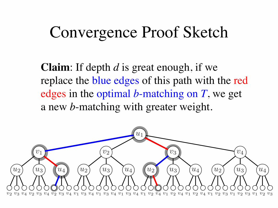
Claim: If depth d is great enough, if we replace the blue edges of this path with the red edges in the optimal b-matching on T, we get a new b-matching with greater weight.
u1
v1 v2 v3 v4
u2 u2 u2 u2u3 u3 u3 u3u4 u4 u4 u4
v2 v3 v4 v2 v3 v4 v2 v3 v4 v1 v3 v4 v1 v3 v4 v1 v3 v4 v1 v2 v4 v1 v2 v4 v1 v2 v4 v1 v2 v3 v1 v2 v3 v1 v2 v3
Figure 2: Example unwrapped graph T of G at 3 iterations. The matching MT is highlighted based on MG from Figure1. Note that leaf nodes cannot have perfect b-matchings, but all inner nodes and the root do. One possible path PT ishighlighted, which is discussed in Lemma ??.
. . .u2v2u4v1u1v3u4v1u3
First cycle
(a) PG
u4
v3u1
v1
(b) c1
. . .u2v2u4v1u3
(c) PG \ c1
Figure 4: (a) One possible extension of PG from Figure 1. This path comes from a deeper T so PG is longer. The firstcycle c1 detected is highlighted. (b) Cycle c1 from PG. (c) The remainder of PG when we remove c1. Note the alternationof the matched edges remains consistent even when we cut out cycles in the interior of the path.
the GOBLIN line). Since both algorithms have run-ning time O(bn3), when we fix b = 5, we get a cubiccurve. When we fix b = n/2, we get a quartic curvebecause b becomes a function of n.
20
40
204060801000
0.1
b
BP median running time
n
t
20
40
204060801000
100
b
GOBLIN median running time
n
t
20 40 60 80 1000
1
2
3
n
t1/3
Median Running time when B=5
20 40 60 80 1000
1
2
3
4
n
t1/4
Median Running time when B=! n/2 "
GOBLIN
BP
GOBLIN
BP
Figure 5: Median running time in seconds on randomlyweighted graphs for the GOBLIN library and BP. Top Left:BP median running time with respect to n, b. Bottom Left:GOBLIN b-matching solver median running time over n,b. Top Right: Cube root of running time ( 3
!t) of both
algorithms when b = 3; note that both scale linearly inthis plot, implying a n3 term in running time for both.Bottom Right: Root-4 ( 4
!t) of running time for various n,
when b = "n/2#. Both algorithms have quartic runningtime.
2.2 b-MATCHING FOR CLASSIFICATION
One natural application of b-matching is as an im-provement over k-nearest neighbor (KNN) for classi-fication. Using KNN for classification is a quick wayof computing a reasonable prediction of class, but it isinherently greedy. The algorithm starts by computingan a!nity matrix between all data points. For eachtest data point, KNN greedily selects its k neighborsregardless of the connectivity or graph this may gener-ate. This invariably leads to some nodes serving as hubnodes and labeling too many unknown examples whileother training points are never used as neighbors.
Instead, using b-matching enforces uniform connectiv-ity across the training and testing points. For exam-ple, assume the number of testing points and trainingpoints is the same and we perform b-matching. Then,each testing point will be labeled by b training pointsand each training point contributes to the labeling ofb testing points. This means b-matching will do a bet-ter job of recreating the distribution of classes seenin the training data when it classifies test data. Thisis useful when test data is transformed in some waythat preserves the shape of the distribution, but it istranslated or scaled to confuse KNN. This can occur insituations where training data comes from a di"erentsource than the testing data.
In both algorithms, we compute a bipartite a!nitygraph between a set of training points and a set oftesting points. We fix the cardinalities of these setsto be equal (though if they are unequal we can down-sample and run the algorithm in multiple folds to ob-
Convergence Proof Sketch
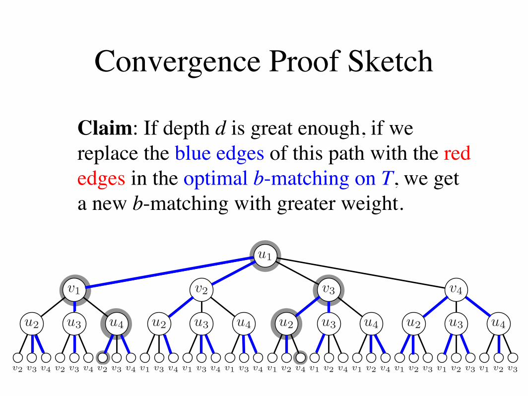
Claim: If depth d is great enough, if we replace the blue edges of this path with the red edges in the optimal b-matching on T, we get a new b-matching with greater weight.
u1
v1 v2 v3 v4
u2 u2 u2 u2u3 u3 u3 u3u4 u4 u4 u4
v2 v3 v4 v2 v3 v4 v2 v3 v4 v1 v3 v4 v1 v3 v4 v1 v3 v4 v1 v2 v4 v1 v2 v4 v1 v2 v4 v1 v2 v3 v1 v2 v3 v1 v2 v3
Figure 2: Example unwrapped graph T of G at 3 iterations. The matching MT is highlighted based on MG from Figure1. Note that leaf nodes cannot have perfect b-matchings, but all inner nodes and the root do. One possible path PT ishighlighted, which is discussed in Lemma ??.
. . .u2v2u4v1u1v3u4v1u3
First cycle
(a) PG
u4
v3u1
v1
(b) c1
. . .u2v2u4v1u3
(c) PG \ c1
Figure 4: (a) One possible extension of PG from Figure 1. This path comes from a deeper T so PG is longer. The firstcycle c1 detected is highlighted. (b) Cycle c1 from PG. (c) The remainder of PG when we remove c1. Note the alternationof the matched edges remains consistent even when we cut out cycles in the interior of the path.
the GOBLIN line). Since both algorithms have run-ning time O(bn3), when we fix b = 5, we get a cubiccurve. When we fix b = n/2, we get a quartic curvebecause b becomes a function of n.
20
40
204060801000
0.1
b
BP median running time
n
t
20
40
204060801000
100
b
GOBLIN median running time
n
t
20 40 60 80 1000
1
2
3
n
t1/3
Median Running time when B=5
20 40 60 80 1000
1
2
3
4
n
t1/4
Median Running time when B=! n/2 "
GOBLIN
BP
GOBLIN
BP
Figure 5: Median running time in seconds on randomlyweighted graphs for the GOBLIN library and BP. Top Left:BP median running time with respect to n, b. Bottom Left:GOBLIN b-matching solver median running time over n,b. Top Right: Cube root of running time ( 3
!t) of both
algorithms when b = 3; note that both scale linearly inthis plot, implying a n3 term in running time for both.Bottom Right: Root-4 ( 4
!t) of running time for various n,
when b = "n/2#. Both algorithms have quartic runningtime.
2.2 b-MATCHING FOR CLASSIFICATION
One natural application of b-matching is as an im-provement over k-nearest neighbor (KNN) for classi-fication. Using KNN for classification is a quick wayof computing a reasonable prediction of class, but it isinherently greedy. The algorithm starts by computingan a!nity matrix between all data points. For eachtest data point, KNN greedily selects its k neighborsregardless of the connectivity or graph this may gener-ate. This invariably leads to some nodes serving as hubnodes and labeling too many unknown examples whileother training points are never used as neighbors.
Instead, using b-matching enforces uniform connectiv-ity across the training and testing points. For exam-ple, assume the number of testing points and trainingpoints is the same and we perform b-matching. Then,each testing point will be labeled by b training pointsand each training point contributes to the labeling ofb testing points. This means b-matching will do a bet-ter job of recreating the distribution of classes seenin the training data when it classifies test data. Thisis useful when test data is transformed in some waythat preserves the shape of the distribution, but it istranslated or scaled to confuse KNN. This can occur insituations where training data comes from a di"erentsource than the testing data.
In both algorithms, we compute a bipartite a!nitygraph between a set of training points and a set oftesting points. We fix the cardinalities of these setsto be equal (though if they are unequal we can down-sample and run the algorithm in multiple folds to ob-
Convergence Proof Sketch
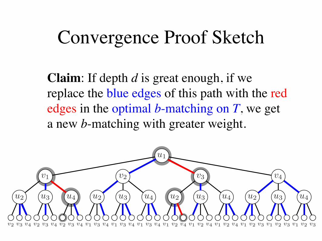
Claim: If depth d is great enough, if we replace the blue edges of this path with the red edges in the optimal b-matching on T, we get a new b-matching with greater weight.
u1
v1 v2 v3 v4
u2 u2 u2 u2u3 u3 u3 u3u4 u4 u4 u4
v2 v3 v4 v2 v3 v4 v2 v3 v4 v1 v3 v4 v1 v3 v4 v1 v3 v4 v1 v2 v4 v1 v2 v4 v1 v2 v4 v1 v2 v3 v1 v2 v3 v1 v2 v3
Figure 2: Example unwrapped graph T of G at 3 iterations. The matching MT is highlighted based on MG from Figure1. Note that leaf nodes cannot have perfect b-matchings, but all inner nodes and the root do. One possible path PT ishighlighted, which is discussed in Lemma ??.
. . .u2v2u4v1u1v3u4v1u3
First cycle
(a) PG
u4
v3u1
v1
(b) c1
. . .u2v2u4v1u3
(c) PG \ c1
Figure 4: (a) One possible extension of PG from Figure 1. This path comes from a deeper T so PG is longer. The firstcycle c1 detected is highlighted. (b) Cycle c1 from PG. (c) The remainder of PG when we remove c1. Note the alternationof the matched edges remains consistent even when we cut out cycles in the interior of the path.
the GOBLIN line). Since both algorithms have run-ning time O(bn3), when we fix b = 5, we get a cubiccurve. When we fix b = n/2, we get a quartic curvebecause b becomes a function of n.
20
40
204060801000
0.1
b
BP median running time
n
t
20
40
204060801000
100
b
GOBLIN median running time
n
t
20 40 60 80 1000
1
2
3
n
t1/3
Median Running time when B=5
20 40 60 80 1000
1
2
3
4
n
t1/4
Median Running time when B=! n/2 "
GOBLIN
BP
GOBLIN
BP
Figure 5: Median running time in seconds on randomlyweighted graphs for the GOBLIN library and BP. Top Left:BP median running time with respect to n, b. Bottom Left:GOBLIN b-matching solver median running time over n,b. Top Right: Cube root of running time ( 3
!t) of both
algorithms when b = 3; note that both scale linearly inthis plot, implying a n3 term in running time for both.Bottom Right: Root-4 ( 4
!t) of running time for various n,
when b = "n/2#. Both algorithms have quartic runningtime.
2.2 b-MATCHING FOR CLASSIFICATION
One natural application of b-matching is as an im-provement over k-nearest neighbor (KNN) for classi-fication. Using KNN for classification is a quick wayof computing a reasonable prediction of class, but it isinherently greedy. The algorithm starts by computingan a!nity matrix between all data points. For eachtest data point, KNN greedily selects its k neighborsregardless of the connectivity or graph this may gener-ate. This invariably leads to some nodes serving as hubnodes and labeling too many unknown examples whileother training points are never used as neighbors.
Instead, using b-matching enforces uniform connectiv-ity across the training and testing points. For exam-ple, assume the number of testing points and trainingpoints is the same and we perform b-matching. Then,each testing point will be labeled by b training pointsand each training point contributes to the labeling ofb testing points. This means b-matching will do a bet-ter job of recreating the distribution of classes seenin the training data when it classifies test data. Thisis useful when test data is transformed in some waythat preserves the shape of the distribution, but it istranslated or scaled to confuse KNN. This can occur insituations where training data comes from a di"erentsource than the testing data.
In both algorithms, we compute a bipartite a!nitygraph between a set of training points and a set oftesting points. We fix the cardinalities of these setsto be equal (though if they are unequal we can down-sample and run the algorithm in multiple folds to ob-
Convergence Proof Sketch
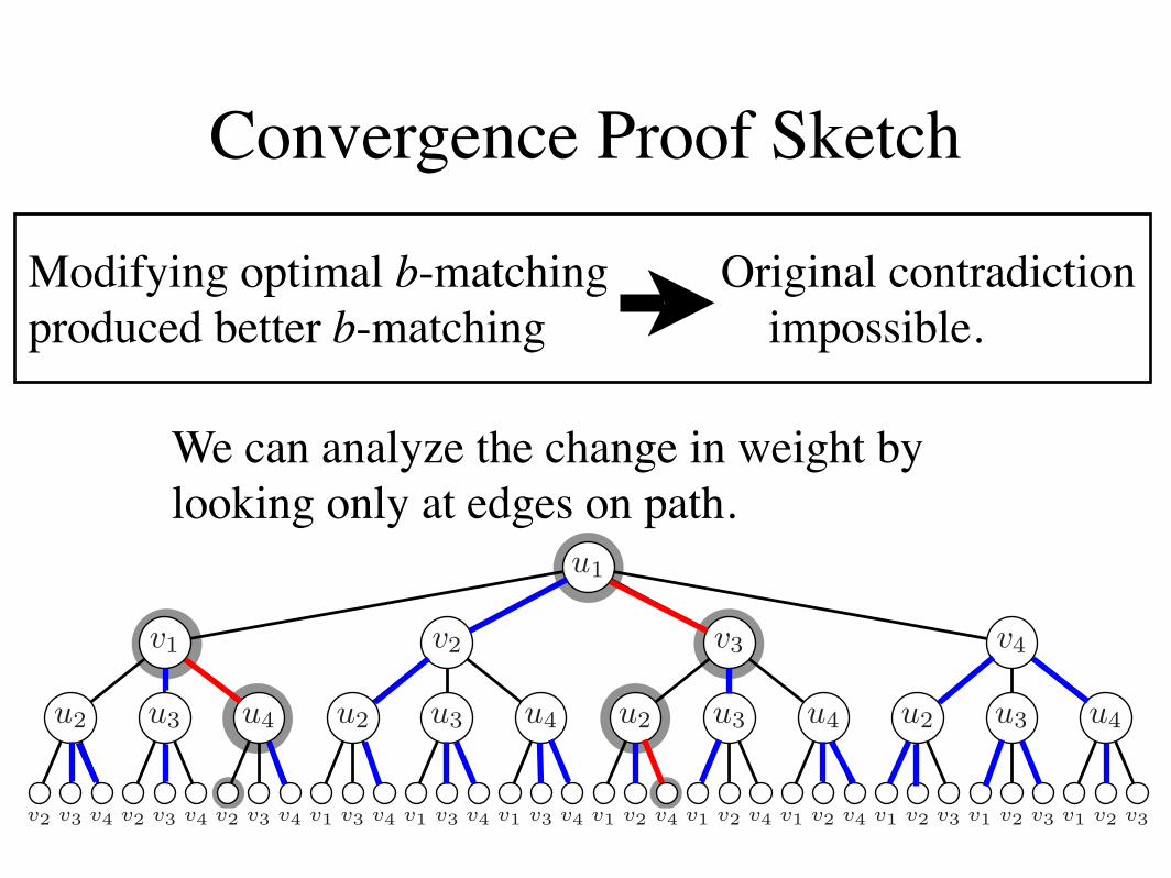
We can analyze the change in weight by looking only at edges on path.
u1
v1 v2 v3 v4
u2 u2 u2 u2u3 u3 u3 u3u4 u4 u4 u4
v2 v3 v4 v2 v3 v4 v2 v3 v4 v1 v3 v4 v1 v3 v4 v1 v3 v4 v1 v2 v4 v1 v2 v4 v1 v2 v4 v1 v2 v3 v1 v2 v3 v1 v2 v3
Figure 2: Example unwrapped graph T of G at 3 iterations. The matching MT is highlighted based on MG from Figure1. Note that leaf nodes cannot have perfect b-matchings, but all inner nodes and the root do. One possible path PT ishighlighted, which is discussed in Lemma ??.
. . .u2v2u4v1u1v3u4v1u3
First cycle
(a) PG
u4
v3u1
v1
(b) c1
. . .u2v2u4v1u3
(c) PG \ c1
Figure 4: (a) One possible extension of PG from Figure 1. This path comes from a deeper T so PG is longer. The firstcycle c1 detected is highlighted. (b) Cycle c1 from PG. (c) The remainder of PG when we remove c1. Note the alternationof the matched edges remains consistent even when we cut out cycles in the interior of the path.
the GOBLIN line). Since both algorithms have run-ning time O(bn3), when we fix b = 5, we get a cubiccurve. When we fix b = n/2, we get a quartic curvebecause b becomes a function of n.
20
40
204060801000
0.1
b
BP median running time
n
t
20
40
204060801000
100
b
GOBLIN median running time
n
t
20 40 60 80 1000
1
2
3
n
t1/3
Median Running time when B=5
20 40 60 80 1000
1
2
3
4
n
t1/4
Median Running time when B=! n/2 "
GOBLIN
BP
GOBLIN
BP
Figure 5: Median running time in seconds on randomlyweighted graphs for the GOBLIN library and BP. Top Left:BP median running time with respect to n, b. Bottom Left:GOBLIN b-matching solver median running time over n,b. Top Right: Cube root of running time ( 3
!t) of both
algorithms when b = 3; note that both scale linearly inthis plot, implying a n3 term in running time for both.Bottom Right: Root-4 ( 4
!t) of running time for various n,
when b = "n/2#. Both algorithms have quartic runningtime.
2.2 b-MATCHING FOR CLASSIFICATION
One natural application of b-matching is as an im-provement over k-nearest neighbor (KNN) for classi-fication. Using KNN for classification is a quick wayof computing a reasonable prediction of class, but it isinherently greedy. The algorithm starts by computingan a!nity matrix between all data points. For eachtest data point, KNN greedily selects its k neighborsregardless of the connectivity or graph this may gener-ate. This invariably leads to some nodes serving as hubnodes and labeling too many unknown examples whileother training points are never used as neighbors.
Instead, using b-matching enforces uniform connectiv-ity across the training and testing points. For exam-ple, assume the number of testing points and trainingpoints is the same and we perform b-matching. Then,each testing point will be labeled by b training pointsand each training point contributes to the labeling ofb testing points. This means b-matching will do a bet-ter job of recreating the distribution of classes seenin the training data when it classifies test data. Thisis useful when test data is transformed in some waythat preserves the shape of the distribution, but it istranslated or scaled to confuse KNN. This can occur insituations where training data comes from a di"erentsource than the testing data.
In both algorithms, we compute a bipartite a!nitygraph between a set of training points and a set oftesting points. We fix the cardinalities of these setsto be equal (though if they are unequal we can down-sample and run the algorithm in multiple folds to ob-
Convergence Proof Sketch
Modifying optimal b-matching produced better b-matching
Original contradiction impossible.
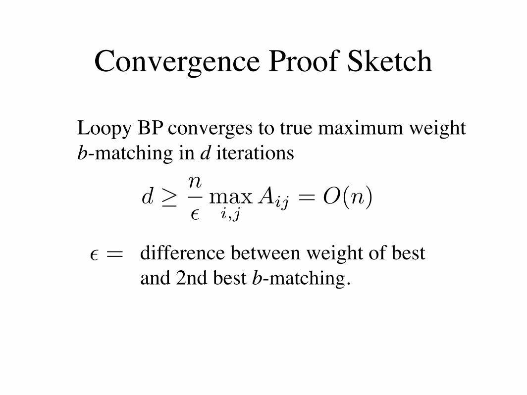
Loopy BP converges to true maximum weight b-matching in d iterations
Convergence Proof Sketch
! = difference between weight of best and 2nd best b-matching.
d !n
!max
i,jAij = O(n)
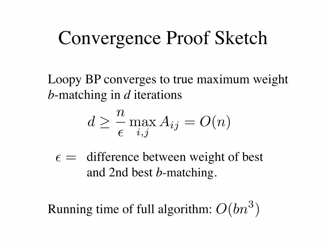
Loopy BP converges to true maximum weight b-matching in d iterations
Running time of full algorithm:
Convergence Proof Sketch
! = difference between weight of best and 2nd best b-matching.
O(bn3)
d !n
!max
i,jAij = O(n)
1. Bipartite Weighted b-Matching
2. Edge Weights As a Distribution
3. Efficient Max-Product
4. Convergence Proof Sketch
5. Experiments
6. Discussion
Outline
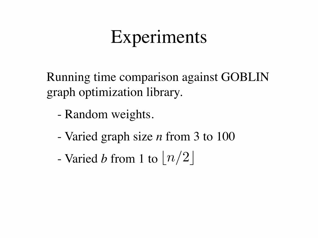
Experiments
Running time comparison against GOBLIN graph optimization library.
- Random weights.
- Varied graph size n from 3 to 100
- Varied b from 1 to !n/2"
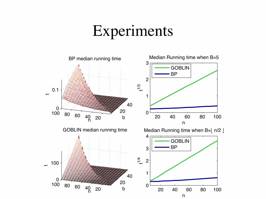
Experiments
Running time comparison against GOBLIN graph optimization library.
. . .u2v2u4v1u1v3u4v1u3
First cycle
(a) PG
u4
v3u1
v1
(b) c1
. . .u2v2u4v1u3
(c) PG \ c1
Figure 4: (a) One possible extension of PG from Figure 4. This path comes from a deeper T so PG is longer. The firstcycle c1 detected is highlighted. (b) Cycle c1 from PG. (c) The remainder of PG when we remove c1. Note the alternationof the matched edges remains consistent even when we cut out cycles in the interior of the path.
with edges in PT toggled, that has a higher weightthan MT . This should be impossible because MT isdefined as the optimal b-matching. This occurs when
d !n
!
!
maxe1,e2!E
W(e1) "W(e2)
"
.
We can consider ! and the maximum di!erence be-tween weights as constants. If d = "(n), Contradic-tion 1 always leads to this impossible circumstance,and therefore Theorem 1 is true.
The bound in this proof is for the worst-case. In ourexperiments, the maximum and minimum weights hadlittle e!ect and the ! term only changed convergencetime noticeably if its value was near zero. Due to finitenumerical precision, this may appear as a tie betweendi!erent settings, which often causes BP to fail [11].
5 EXPERIMENTS
We elaborate the speed advantages of our method andan application in machine learning where b-matchingcan improve classification accuracy.
5.1 RUNNING TIME ANALYSIS
We compare the performance of our implementationof belief propagation maximum weighted b-matchingagainst the free graph optimization package, GOBLIN.1
Classical b-matching algorithms such as the balancednetwork flow method used by the GOBLIN library runin O(bn3) time [2]. The belief propagation methodtakes O(bn) time to compute one iteration of messageupdates for each of the 2n nodes and converges in O(n)iterations. So, its overall running time is also O(bn3).
We ran both algorithms on randomly generated bipar-tite graphs of 10 # n # 100 and 1 # b # n/2. Wegenerated the weight matrix with the rand functionin MATLAB, which picks each weight independentlyfrom a uniform distribution between 0 and 1.
1Available at: http://www.math.uni-augsburg.de/opt/goblin.html
The GOBLIN library is C++ code and our implemen-tation2 of belief propagation b-matching is in C. Bothwere run on a 3.00 Ghz. Pentium 4 processor.
In general, the belief propagation runs hundreds oftimes faster than GOBLIN. Figure 5 shows variouscomparisons of their running times. The surface plotsshow how the algorithms scale with respect to n andb. The line plots show cross sections of these surfaceplots, with appropriate transformations on the run-ning time to show the scaling (without these transfor-mations, the belief propagation line would appear tobe always zero due to the scale of the plot followingthe GOBLIN line). Since both algorithms have run-ning time O(bn3), when we fix b = 5, we get a cubiccurve. When we fix b = n/2, we get a quartic curvebecause b becomes a function of n.
20
40
204060801000
0.1
b
BP median running time
n
t
20
40
204060801000
100
b
GOBLIN median running time
n
t
20 40 60 80 1000
1
2
3
n
t1/3
Median Running time when B=5
20 40 60 80 1000
1
2
3
4
n
t1/4
Median Running time when B=! n/2 "
GOBLIN
BP
GOBLIN
BP
Figure 5: Median running time in seconds on randomlyweighted graphs for the GOBLIN library and BP. Top Left:BP median running time with respect to n, b. Bottom Left:GOBLIN b-matching solver median running time over n,b. Top Right: Cube root of running time ( 3
!t) of both
algorithms when b = 3; note that both scale linearly inthis plot, implying a n3 term in running time for both.Bottom Right: Root-4 ( 4
!t) of running time for various n,
when b = "n/2#. Both algorithms have quartic runningtime.
2Available at http://www.cs.columbia.edu/bert/bmatching
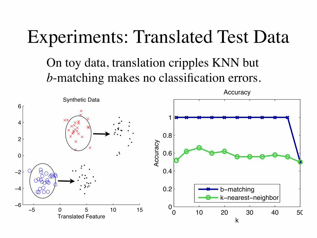
Experiments: Translated Test DataOn toy data, translation cripples KNN but b-matching makes no classification errors.
u1 u2 u3 u4
v1 v2 v3 v4
1,5 234 6
Figure 5: The cyclic alternating path PG starting at v1 onG that corresponds to the nodes visited by PT . Edges arenumbered to help follow the loopy path.
20
40
204060801000
0.1
b
BP median running time
n
t
20
40
204060801000
100
b
GOBLIN median running time
n
t
20 40 60 80 1000
1
2
3
n
t1/3
Median Running time when B=5
20 40 60 80 1000
1
2
3
4
n
t1/4
Median Running time when B=! n/2 "
GOBLIN
BP
GOBLIN
BP
Figure 7: Median running time in seconds on randomlyweighted graphs for the GOBLIN library and BP. Top Left:BP median running time with respect to n, b. Bottom Left:GOBLIN b-matching solver median running time over n,b. Top Right: Cube root of running time ( 3
!t) of both
algorithms when b = 3; note that both scale linearly inthis plot, implying a n3 term in running time for both.Bottom Right: Root-4 ( 4
!t) of running time for various n,
when b = "n/2#. Both algorithms have quartic runningtime.
of computing a reasonable prediction of class, but it isinherently greedy. The algorithm starts by computingan a!nity matrix between all data points. For eachtest data point, KNN greedily selects its k neighborsregardless of the connectivity or graph this may gener-ate. This invariably leads to some nodes serving as hubnodes and labeling too many unknown examples whileother training points are never used as neighbors.
Instead, using b-matching enforces uniform connectiv-ity across the training and testing points. For exam-ple, assume the number of testing points and trainingpoints is the same and we perform b-matching. Then,each testing point will be labeled by b training pointsand each training point contributes to the labeling ofb testing points. This means b-matching will do a bet-ter job of recreating the distribution of classes seenin the training data when it classifies test data. Thisis useful when test data is transformed in some waythat preserves the shape of the distribution, but it is
!10 !5 0 5 10 15!6
!4
!2
0
2
4
6Synthetic Data
Translated Feature0 10 20 30 40 50
0
0.2
0.4
0.6
0.8
1
k
Accura
cy
Accuracy
Train +1
Test +1
Train !1
Test !1
b!matching
k!nearest!neighbor
Figure 8: Left: Synthetic classification data where the testdata is translated to the right along the x-axis. Right: Ac-curacy for k-nearest neighbor versus b-matching for variousk (or b).
translated or scaled to confuse KNN. This can occur insituations where training data comes from a di"erentsource than the testing data.
In both algorithms, we compute a bipartite a!nitygraph between a set of training points and a set oftesting points. We fix the cardinalities of these setsto be equal (though if they are unequal we can down-sample and run the algorithm in multiple folds to ob-tain classifications). We use either KNN or weightedb-matching to prune the graph, then we classify eachtest point based on the majority of the classes of theneighbors. In our experiments, we use negative Eu-clidean distance as our a!nity metric.
2.2.1 Synthetic Data
We created synthetic data by sampling 50 trainingdata points from two spherical Gaussians with meansat (3, 3) and (!3,!3). We then sampled 50 testingdata points from similar Gaussians, but translatedalong the x-axis by +8. This is a severe case of trans-lation where it is obvious that KNN could be fooled bythe proximity of the testing Gaussian to the trainingGaussian of the wrong class. Figure 7 shows the pointswe sampled from this setup. As expected, KNN couldonly achieve 65% accuracy on this data for the opti-mal setting of k, while b-matching classified the pointsperfectly for all settings of b.
2.2.2 MNIST Digits With Backgrounds
We sampled the MNIST digits dataset of 28 " 28grayscale digits. For each of the digits 3, 5, and 8,we sampled 100 training points from the training setand 100 from the testing set. We average accuracyover 20 random samplings to avoid anomalous results.We cross-validate over settings of b and k in the range[1, 300] and save the best accuracy achieved for eachalgorithm on each sampling.
We examine the case where training and testing data
!! " ! #" #!!$
!%
!&
"
&
%
$'()*+,*-./01*1
231)451*,6/7,1*83,
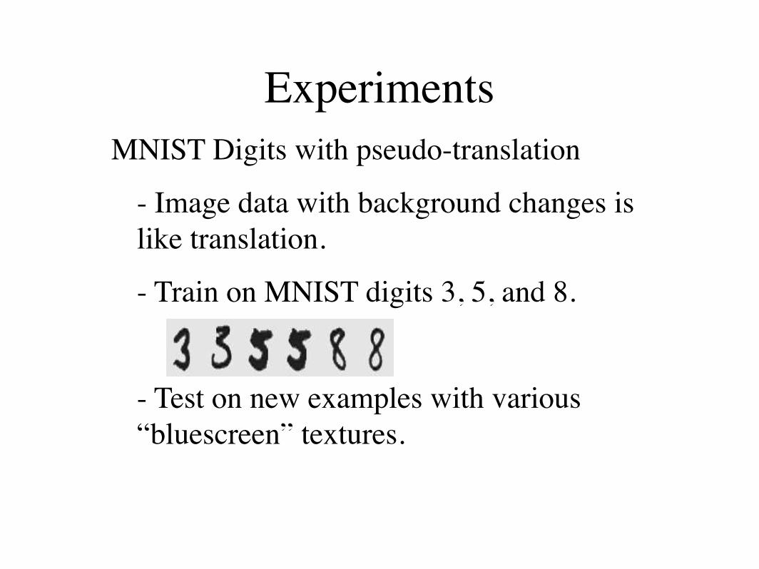
ExperimentsMNIST Digits with pseudo-translation
- Image data with background changes is like translation.
- Train on MNIST digits 3, 5, and 8.
- Test on new examples with various “bluescreen” textures.
lem. We provided an e!cient method to update the!
nb
"
-length messages. The practical running time ofthis algorithm is hundreds of times faster than theclassical implementations we have found. This makesb-matching a more practical tool in machine learningsettings and lets us tackle significantly larger datasets.
Furthermore, by formulating weighted b-matching inthis manner, we can take advantage of the inherentparallel computation of belief propagation. In addi-tion to the empirical evidence of a faster constant onthe asymptotic running time, the procedure could bedistributed over a number of machines. For example,n servers and n clients could run this algorithm in par-allel to optimize throughput.
Theoretically, the convergence of loopy BP on thisgraph and the ability to update the
!nb
"
length mes-sages are pleasant surprises. We have tried to gen-eralize this method to all graph structures, not justbipartite graphs, but found that there were cases thatled to oscillation in the belief updates. This is due tothe fact that cycles can be both even and odd in gen-eral graphs. Generalizing to such cases is one futuredirection for this work.
In addition to being limited to bipartite graphs, be-lief propagation methods have di!culty with functionsthat have multiple solutions. This is why we assumethere is a unique solution in the proof. In a way, ourconvergence bound still holds when there are multi-ple solutions, in the sense that the ! value is in thedenominator, so the limit as ! goes to zero impliesinfinite iterations to convergence. Belief propagationcannot handle these ties in the function due to the factthat the information being passed between variables isonly the maximum value, and no information aboutthe actual variable values is sent. Therefore, the al-gorithm has no mechanism to distinguish between onemaximum and the other. We are currently investi-gating if tree-based reparameterization techniques orother graphical model inference methods can solve themultiple-optimum or non-bipartite b-matching cases.
Acknowledgments
We thank Stuart Andrews, Andrew Howard and BlakeShaw for insightful discussions. Supported in part byNSF grant IIS-0347499.
References
[1] M. Bayati, D. Shah, and M. Sharma. Maximumweight matching via max-product belief propagation.In Proc. of the IEEE International Symposium on In-formation Theory, 2005.
[2] C. Fremuth-Paeger and D. Jungnickel. Balanced net-work flows. i. a unifying framework for design and
1 2 3 4 5 6 70
0.2
0.4
0.6
0.8
1
Background texture
Ave
rag
e a
ccu
racy BM
KNN
100 200 3000
0.2
0.4
0.6
0.8
1
k
Ave
rag
e a
ccu
racy BM
KNN
1
2
3
4
5
6
7
Figure 7: (Left) Examples of digits placed on back-grounds: 1-unaltered, 2-diagonal lines, 3-grid, 4-whitenoise, 5-brushed metal, 6-wood, 7-marble. (Top right) Av-erage accuracies over 20 random samplings for optimal set-ting of b or k. (Bottom right) Average accuracy on woodbackground for various settings of b or k.
analysis of matching algorithms. Networks, 33(1):1–28, 1999.
[3] B. Frey and D. Dueck. Mixture modeling by a!nitypropagation. In Advances in Neural Information Pro-cessing Systems 18, pages 379–386. MIT Press, 2006.
[4] T. Jebara and V. Shchogolev. B-matching for spectralclustering. In Proc. of the European Conference onMachine Learning, ECML, 2006.
[5] J. Mooij and H. Kappen. Su!cient conditions for con-vergence of loopy belief propagation. In Proceedingsof the 21th Annual Conference on Uncertainty in Ar-tificial Intelligence (UAI-05), pages 396–40, 2005.
[6] M. Muller-Hannemann and A. Schwartz. Implement-ing weighted b-matching algorithms: Insights from acomputational study. In ACM Journal of Experimen-tal Algorithmics, Volume 5, Article 8, 2000.
[7] J. Pearl. Probabilistic reasoning in intelligent systems:networks of plausible inference. Morgan KaufmannPublishers Inc., San Francisco, CA, USA, 1988.
[8] S. Tatikonda and M. Jordan. Loopy belief propagationand Gibbs measures. In Proc. Uncertainty in ArtificialIntell., vol. 18, 2002.
[9] M. J. Wainwright, T. Jaakkola, and A. S. Willsky.Tree-based reparameterization framework for analysisof sum-product and related algorithms. IEEE Trans-actions on Information Theory, 49(5), 2003.
[10] Y. Weiss. Correctness of local probability propagationin graphical models with loops. Neural Computation,12(1):1–41, 2000.
[11] Y. Weiss and W. Freeman. On the optimality of solu-tions of the max-product belief-propagation algorithmin arbitrary graphs. IEEETIT: IEEE Transactions onInformation Theory, 47, 2001.
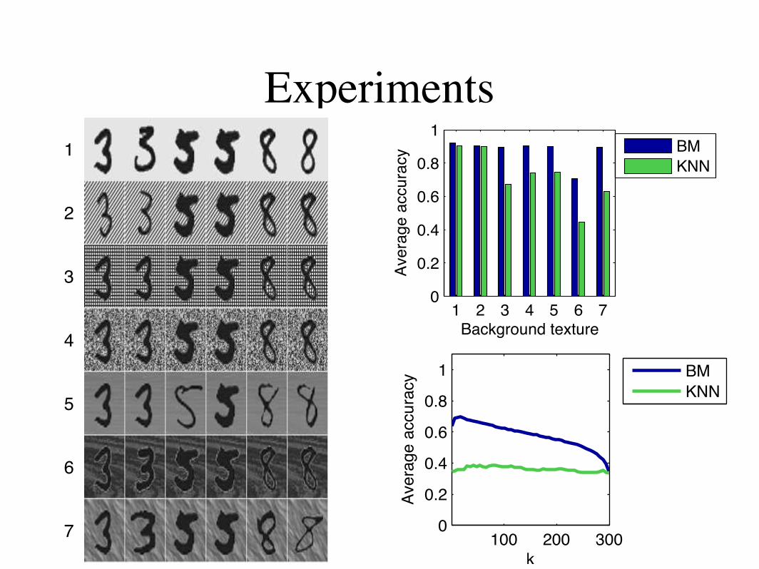
Experimentslem. We provided an e!cient method to update the!
nb
"
-length messages. The practical running time ofthis algorithm is hundreds of times faster than theclassical implementations we have found. This makesb-matching a more practical tool in machine learningsettings and lets us tackle significantly larger datasets.
Furthermore, by formulating weighted b-matching inthis manner, we can take advantage of the inherentparallel computation of belief propagation. In addi-tion to the empirical evidence of a faster constant onthe asymptotic running time, the procedure could bedistributed over a number of machines. For example,n servers and n clients could run this algorithm in par-allel to optimize throughput.
Theoretically, the convergence of loopy BP on thisgraph and the ability to update the
!nb
"
length mes-sages are pleasant surprises. We have tried to gen-eralize this method to all graph structures, not justbipartite graphs, but found that there were cases thatled to oscillation in the belief updates. This is due tothe fact that cycles can be both even and odd in gen-eral graphs. Generalizing to such cases is one futuredirection for this work.
In addition to being limited to bipartite graphs, be-lief propagation methods have di!culty with functionsthat have multiple solutions. This is why we assumethere is a unique solution in the proof. In a way, ourconvergence bound still holds when there are multi-ple solutions, in the sense that the ! value is in thedenominator, so the limit as ! goes to zero impliesinfinite iterations to convergence. Belief propagationcannot handle these ties in the function due to the factthat the information being passed between variables isonly the maximum value, and no information aboutthe actual variable values is sent. Therefore, the al-gorithm has no mechanism to distinguish between onemaximum and the other. We are currently investi-gating if tree-based reparameterization techniques orother graphical model inference methods can solve themultiple-optimum or non-bipartite b-matching cases.
Acknowledgments
We thank Stuart Andrews, Andrew Howard and BlakeShaw for insightful discussions. Supported in part byNSF grant IIS-0347499.
References
[1] M. Bayati, D. Shah, and M. Sharma. Maximumweight matching via max-product belief propagation.In Proc. of the IEEE International Symposium on In-formation Theory, 2005.
[2] C. Fremuth-Paeger and D. Jungnickel. Balanced net-work flows. i. a unifying framework for design and
1 2 3 4 5 6 70
0.2
0.4
0.6
0.8
1
Background textureA
ve
rag
e a
ccu
racy BM
KNN
100 200 3000
0.2
0.4
0.6
0.8
1
k
Ave
rag
e a
ccu
racy BM
KNN
1
2
3
4
5
6
7
Figure 7: (Left) Examples of digits placed on back-grounds: 1-unaltered, 2-diagonal lines, 3-grid, 4-whitenoise, 5-brushed metal, 6-wood, 7-marble. (Top right) Av-erage accuracies over 20 random samplings for optimal set-ting of b or k. (Bottom right) Average accuracy on woodbackground for various settings of b or k.
analysis of matching algorithms. Networks, 33(1):1–28, 1999.
[3] B. Frey and D. Dueck. Mixture modeling by a!nitypropagation. In Advances in Neural Information Pro-cessing Systems 18, pages 379–386. MIT Press, 2006.
[4] T. Jebara and V. Shchogolev. B-matching for spectralclustering. In Proc. of the European Conference onMachine Learning, ECML, 2006.
[5] J. Mooij and H. Kappen. Su!cient conditions for con-vergence of loopy belief propagation. In Proceedingsof the 21th Annual Conference on Uncertainty in Ar-tificial Intelligence (UAI-05), pages 396–40, 2005.
[6] M. Muller-Hannemann and A. Schwartz. Implement-ing weighted b-matching algorithms: Insights from acomputational study. In ACM Journal of Experimen-tal Algorithmics, Volume 5, Article 8, 2000.
[7] J. Pearl. Probabilistic reasoning in intelligent systems:networks of plausible inference. Morgan KaufmannPublishers Inc., San Francisco, CA, USA, 1988.
[8] S. Tatikonda and M. Jordan. Loopy belief propagationand Gibbs measures. In Proc. Uncertainty in ArtificialIntell., vol. 18, 2002.
[9] M. J. Wainwright, T. Jaakkola, and A. S. Willsky.Tree-based reparameterization framework for analysisof sum-product and related algorithms. IEEE Trans-actions on Information Theory, 49(5), 2003.
[10] Y. Weiss. Correctness of local probability propagationin graphical models with loops. Neural Computation,12(1):1–41, 2000.
[11] Y. Weiss and W. Freeman. On the optimality of solu-tions of the max-product belief-propagation algorithmin arbitrary graphs. IEEETIT: IEEE Transactions onInformation Theory, 47, 2001.
lem. We provided an e!cient method to update the!
nb
"
-length messages. The practical running time ofthis algorithm is hundreds of times faster than theclassical implementations we have found. This makesb-matching a more practical tool in machine learningsettings and lets us tackle significantly larger datasets.
Furthermore, by formulating weighted b-matching inthis manner, we can take advantage of the inherentparallel computation of belief propagation. In addi-tion to the empirical evidence of a faster constant onthe asymptotic running time, the procedure could bedistributed over a number of machines. For example,n servers and n clients could run this algorithm in par-allel to optimize throughput.
Theoretically, the convergence of loopy BP on thisgraph and the ability to update the
!nb
"
length mes-sages are pleasant surprises. We have tried to gen-eralize this method to all graph structures, not justbipartite graphs, but found that there were cases thatled to oscillation in the belief updates. This is due tothe fact that cycles can be both even and odd in gen-eral graphs. Generalizing to such cases is one futuredirection for this work.
In addition to being limited to bipartite graphs, be-lief propagation methods have di!culty with functionsthat have multiple solutions. This is why we assumethere is a unique solution in the proof. In a way, ourconvergence bound still holds when there are multi-ple solutions, in the sense that the ! value is in thedenominator, so the limit as ! goes to zero impliesinfinite iterations to convergence. Belief propagationcannot handle these ties in the function due to the factthat the information being passed between variables isonly the maximum value, and no information aboutthe actual variable values is sent. Therefore, the al-gorithm has no mechanism to distinguish between onemaximum and the other. We are currently investi-gating if tree-based reparameterization techniques orother graphical model inference methods can solve themultiple-optimum or non-bipartite b-matching cases.
Acknowledgments
We thank Stuart Andrews, Andrew Howard and BlakeShaw for insightful discussions. Supported in part byNSF grant IIS-0347499.
References
[1] M. Bayati, D. Shah, and M. Sharma. Maximumweight matching via max-product belief propagation.In Proc. of the IEEE International Symposium on In-formation Theory, 2005.
[2] C. Fremuth-Paeger and D. Jungnickel. Balanced net-work flows. i. a unifying framework for design and
1 2 3 4 5 6 70
0.2
0.4
0.6
0.8
1
Background texture
Ave
rag
e a
ccu
racy BM
KNN
100 200 3000
0.2
0.4
0.6
0.8
1
k
Ave
rag
e a
ccu
racy BM
KNN
1
2
3
4
5
6
7
Figure 7: (Left) Examples of digits placed on back-grounds: 1-unaltered, 2-diagonal lines, 3-grid, 4-whitenoise, 5-brushed metal, 6-wood, 7-marble. (Top right) Av-erage accuracies over 20 random samplings for optimal set-ting of b or k. (Bottom right) Average accuracy on woodbackground for various settings of b or k.
analysis of matching algorithms. Networks, 33(1):1–28, 1999.
[3] B. Frey and D. Dueck. Mixture modeling by a!nitypropagation. In Advances in Neural Information Pro-cessing Systems 18, pages 379–386. MIT Press, 2006.
[4] T. Jebara and V. Shchogolev. B-matching for spectralclustering. In Proc. of the European Conference onMachine Learning, ECML, 2006.
[5] J. Mooij and H. Kappen. Su!cient conditions for con-vergence of loopy belief propagation. In Proceedingsof the 21th Annual Conference on Uncertainty in Ar-tificial Intelligence (UAI-05), pages 396–40, 2005.
[6] M. Muller-Hannemann and A. Schwartz. Implement-ing weighted b-matching algorithms: Insights from acomputational study. In ACM Journal of Experimen-tal Algorithmics, Volume 5, Article 8, 2000.
[7] J. Pearl. Probabilistic reasoning in intelligent systems:networks of plausible inference. Morgan KaufmannPublishers Inc., San Francisco, CA, USA, 1988.
[8] S. Tatikonda and M. Jordan. Loopy belief propagationand Gibbs measures. In Proc. Uncertainty in ArtificialIntell., vol. 18, 2002.
[9] M. J. Wainwright, T. Jaakkola, and A. S. Willsky.Tree-based reparameterization framework for analysisof sum-product and related algorithms. IEEE Trans-actions on Information Theory, 49(5), 2003.
[10] Y. Weiss. Correctness of local probability propagationin graphical models with loops. Neural Computation,12(1):1–41, 2000.
[11] Y. Weiss and W. Freeman. On the optimality of solu-tions of the max-product belief-propagation algorithmin arbitrary graphs. IEEETIT: IEEE Transactions onInformation Theory, 47, 2001.
lem. We provided an e!cient method to update the!
nb
"
-length messages. The practical running time ofthis algorithm is hundreds of times faster than theclassical implementations we have found. This makesb-matching a more practical tool in machine learningsettings and lets us tackle significantly larger datasets.
Furthermore, by formulating weighted b-matching inthis manner, we can take advantage of the inherentparallel computation of belief propagation. In addi-tion to the empirical evidence of a faster constant onthe asymptotic running time, the procedure could bedistributed over a number of machines. For example,n servers and n clients could run this algorithm in par-allel to optimize throughput.
Theoretically, the convergence of loopy BP on thisgraph and the ability to update the
!nb
"
length mes-sages are pleasant surprises. We have tried to gen-eralize this method to all graph structures, not justbipartite graphs, but found that there were cases thatled to oscillation in the belief updates. This is due tothe fact that cycles can be both even and odd in gen-eral graphs. Generalizing to such cases is one futuredirection for this work.
In addition to being limited to bipartite graphs, be-lief propagation methods have di!culty with functionsthat have multiple solutions. This is why we assumethere is a unique solution in the proof. In a way, ourconvergence bound still holds when there are multi-ple solutions, in the sense that the ! value is in thedenominator, so the limit as ! goes to zero impliesinfinite iterations to convergence. Belief propagationcannot handle these ties in the function due to the factthat the information being passed between variables isonly the maximum value, and no information aboutthe actual variable values is sent. Therefore, the al-gorithm has no mechanism to distinguish between onemaximum and the other. We are currently investi-gating if tree-based reparameterization techniques orother graphical model inference methods can solve themultiple-optimum or non-bipartite b-matching cases.
Acknowledgments
We thank Stuart Andrews, Andrew Howard and BlakeShaw for insightful discussions. Supported in part byNSF grant IIS-0347499.
References
[1] M. Bayati, D. Shah, and M. Sharma. Maximumweight matching via max-product belief propagation.In Proc. of the IEEE International Symposium on In-formation Theory, 2005.
[2] C. Fremuth-Paeger and D. Jungnickel. Balanced net-work flows. i. a unifying framework for design and
1 2 3 4 5 6 70
0.2
0.4
0.6
0.8
1
Background texture
Ave
rage a
ccura
cy BM
KNN
100 200 3000
0.2
0.4
0.6
0.8
1
k
Avera
ge a
ccura
cy BM
KNN
1
2
3
4
5
6
7
Figure 7: (Left) Examples of digits placed on back-grounds: 1-unaltered, 2-diagonal lines, 3-grid, 4-whitenoise, 5-brushed metal, 6-wood, 7-marble. (Top right) Av-erage accuracies over 20 random samplings for optimal set-ting of b or k. (Bottom right) Average accuracy on woodbackground for various settings of b or k.
analysis of matching algorithms. Networks, 33(1):1–28, 1999.
[3] B. Frey and D. Dueck. Mixture modeling by a!nitypropagation. In Advances in Neural Information Pro-cessing Systems 18, pages 379–386. MIT Press, 2006.
[4] T. Jebara and V. Shchogolev. B-matching for spectralclustering. In Proc. of the European Conference onMachine Learning, ECML, 2006.
[5] J. Mooij and H. Kappen. Su!cient conditions for con-vergence of loopy belief propagation. In Proceedingsof the 21th Annual Conference on Uncertainty in Ar-tificial Intelligence (UAI-05), pages 396–40, 2005.
[6] M. Muller-Hannemann and A. Schwartz. Implement-ing weighted b-matching algorithms: Insights from acomputational study. In ACM Journal of Experimen-tal Algorithmics, Volume 5, Article 8, 2000.
[7] J. Pearl. Probabilistic reasoning in intelligent systems:networks of plausible inference. Morgan KaufmannPublishers Inc., San Francisco, CA, USA, 1988.
[8] S. Tatikonda and M. Jordan. Loopy belief propagationand Gibbs measures. In Proc. Uncertainty in ArtificialIntell., vol. 18, 2002.
[9] M. J. Wainwright, T. Jaakkola, and A. S. Willsky.Tree-based reparameterization framework for analysisof sum-product and related algorithms. IEEE Trans-actions on Information Theory, 49(5), 2003.
[10] Y. Weiss. Correctness of local probability propagationin graphical models with loops. Neural Computation,12(1):1–41, 2000.
[11] Y. Weiss and W. Freeman. On the optimality of solu-tions of the max-product belief-propagation algorithmin arbitrary graphs. IEEETIT: IEEE Transactions onInformation Theory, 47, 2001.
1. Bipartite Weighted b-Matching
2. Edge Weights As a Distribution
3. Efficient Max-Product
4. Convergence Proof Sketch
5. Experiments
6. Discussion
Outline
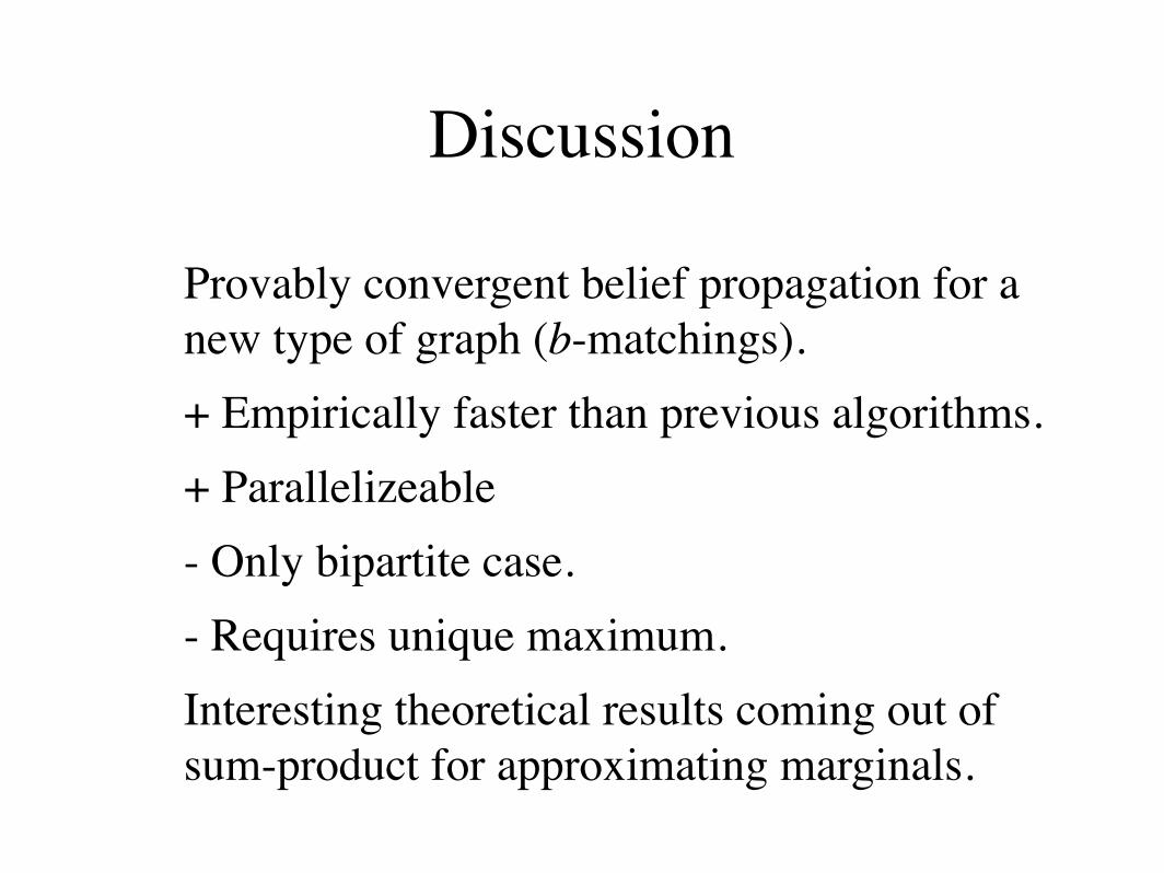
Discussion
Provably convergent belief propagation for a new type of graph (b-matchings). + Empirically faster than previous algorithms.+ Parallelizeable- Only bipartite case.- Requires unique maximum.Interesting theoretical results coming out of sum-product for approximating marginals.