1

LONGITUDINALLY JOINTED EDGE-WISE COMPRESSION HONEYCOMB COMPOSITE SANDWICH COUPON TESTING

AND FE ANALYSIS: THREE METHODS OF STRAIN MEASUREMENT, AND COMPARISON

Babak Farrokh1, Nur Aida Abdul Rahim2, Ken Segal3, Terry Fan1, Justin Jones4, Ken Hodges4, Noah

Mashni2, Naman Garg2, and Alex Sang

2

1NASA Goddard Space Flight Center, Mechanical Systems Analysis and Simulations Branch 2Luna Innovations, Inc.

3NASA Goddard Space Flight Center, Mechanical Engineering Branch 4

NASA Goddard Space Flight Center, Materials Engineering Branch

ABSTRACT

Three distinct strain measurement methods (i.e., foil resistance strain gages, fiber optic strain sensors, and a three-dimensional digital image photogrammetry that gives full field strain and displacement measurements) were implemented to measure strains on the back and front surfaces of a longitudinally jointed curved test article subjected to edge-wise compression testing, at NASA Goddard Space Flight Center, according to ASTM C364.

The pre-test finite element analysis (FEA) was conducted to assess ultimate failure load and predict strain distribution pattern throughout the test coupon. The predicted strain pattern contours were then utilized as guidelines for installing the strain measurement instrumentations.

The foil resistance strain gages and fiber optic strain sensors were bonded on the specimen at locations with nearly the same analytically predicted strain values, and as close as possible to each other, so that, comparisons between the measured strains by strain gages and fiber optic sensors, as well as the three-dimensional digital image photogrammetric system are relevant.

The test article was loaded to failure (at ~167 kN), at the compressive strain value of ~10,000 μɛ. As a part of this study, the validity of the measured strains by fiber optic sensors is examined against the foil resistance strain gages and the three-dimensional digital image photogrammetric data, and comprehensive comparisons are made with FEA predictions.

1. INTRODUCTION Strain measurements are frequently used to verify structural analyses predictions and assess structural designs. Foil resistance strain gages (herein referred to as resistive strain gages) are the strain gage of convention and are used widely in industrial and aerospace applications; from complete structures down to small test coupons. Over the past few decades a number of alternative strain measurement methods have developed which have merit for composite research; namely, 3D photogrammetry (e.g., digital image correlation - DIC) and fiber optic strain sensing. In an effort to make a strain measurement method comparison, an edgewise compression (EWC) specimen per ASTM 364 is used to assess an out-of-autoclave cured fiber reinforced polymer composite bonded joint. This specimen was fabricated based on a design

https://ntrs.nasa.gov/search.jsp?R=20130011719 2019-04-10T21:37:57+00:00Z

2

concept for a Space Launch System (SLS) fairing during the Composites for Exploration (CoEx) effort, and offers sufficient complexity necessary to fully compare and contrast these strain measurement techniques. The EWC tests of highly loaded structures require lateral end supports to spread the load into the test article to prevent end failures, and although the external load is uni-axial in nature, the strain distribution pattern is complex throughout the specimen due to these end conditions and the joint architecture (Figure 1).

Figure 1: Jointed EWC axial strain contour predicted by finite element analysis (FEA).

High mechanical testing costs coupled with fast-paced project timelines often require engineers to minimize the number of mechanical tests and maximize the analytical benefit to data collected. Due to the inherent complexity of structural composite tests such as the EWC geometry, it could be advantageous to either complement or replace conventional strain gages with fiber optic sensors or DIC. While the use of resistive strain gages can be very helpful in balancing the load prior to a test and also as a source for high-resolution measurement in particular regions of interest, DIC and fiber optics offer the ability to monitor strain across the entire surface of the test article. This can be very helpful in validating design models and better understanding failure mechanisms; however, DIC and fiber optic measurement systems have considerably higher upfront costs and require more time and resources for data processing. This case study is intended to provide a real-world comparison between measurement techniques to aid in cost-benefit decisions for future tests of EWC or similarly complex structures.

While resistive strain gages have historically been the method of choice for measuring strain on composite surfaces for their high reliability and precision, they suffer from the disadvantages of providing only single point data over a small area and can be cumbersome and time consuming when multiple resistive strain gages are used. Also, they require bonding to the surface—which may affect properties in thin materials—and can be limited to relatively low total elongations.

Fiber optic sensing has proven valuable for measuring strain due to its ability to measure distributed strain along a structure [Guemes; Kaplan; Klute; Pedrazzani; Pedrazzani]. However, the logistics of managing the resultant large datasets is challenging, and care needs to be taken to protect the fiber sensor as damage to one fiber can obliterate 100 strain sensors on a 1 m strand.

mm/mm

3

The DIC technique is a non-contact measurement that provides full field strain information over an entire surface, but suffers from lower resolution when compared to resistive or optical fiber strain gages, involves surface preparation, and requires an unobstructed optical field of view.

In this work, all three methods of strain sensing, described above, were used to monitor strain during EWC testing of a composite jointed panel: resistive strain gages, fiber optic strain sensing, and three-dimensional DIC. The strain from each technique is compared to the FEA model in order to correlate data between these three measurement methodologies.

2. TEST ARTICLE, INSTRUMENTATION, AND TESTING

2.1. Test Article The CoEx joints team developed an out-of-autoclave composite splice joint for honeycomb sandwich panels for the Space Launch System fairing. An Edgewise Compression (EWC) specimen per ASTM C364: Standard Test Method for Edgewise Compressive Strength of Sandwich Constructions

The jointed EWC panel's parent material is from a 1/16

was prepared for testing to validate the design. th

Segments of this parent panel were provided to the CoEx Joints team. One panel segment 736.6 mm tall by 152.4 mm wide was cut in two and re-joined to simulate a SLS fairing longitudinal joint. The panel seam was first injected with a Hysol 9396.6MD adhesive filling the cut (< 2.5 mm) for vacuum integrity. The joint splice plate was made using Cytec T40-800/5320-1 4-harness satin weave fabric prepreg. The splice plate was enclosed in a vacuum bag, and vacuum and heat were applied to cure the splice plate to the sandwich panels. A schematic of the bonded joint is shown in Figure 2.

arc segments of 10-m diameter cylinder. The panel is sandwich construction. The face-sheets are constructed with Cytec’s IM7/977-3 unidirectional prepreg with an 8-ply quasi-isotropic laminate design. The outer mold line (OML) face-sheet was laminated on a 5m radius concave composite tool using an automated tape laying process. A layer of FM300M film adhesive was placed on the face-sheet followed by an 25.4 mm thick perforated aluminum (5052) core having 3.2 mm hexagonal cell size and .017 mm foil thickness. The second layer of film adhesive was applied to the core, then the inner mold line (IML) face-sheet was laid-up on the film adhesive using the automated tape laying process. The face-sheets and core adhesive were cured in a single autoclave cycle. Face-sheet tensile tests and sandwich flat-wise tension tests validated the panel’s processing quality was better than satisfactory.

Figure 2: Test panel cross section.

4

The cured jointed panel was cut into 4 subsections 177.8 mm tall by 127 mm wide. The width is was effectively 25.4 mm wider than the joint leaving acreage face-sheet available for instrumentation. End support plates (Figure 3) were added to stabilize the face-sheets and prevent local crushing thus generating a predictable and repeatable end condition. Those slotted aluminum end plates allowed a clearance of 12.7 mm all the way around the jointed panel subsections. The jointed subsections were centered and squared in the slot, then and filled with epoxy and cured at room temperature. After the epoxy cured, the specimen ends were machined flat and parallel to within ±0.06 mm. The EWC coupon was ready for instrumentation.

Figure 3: Test coupon assembly prior to instrumentation.

2.2. Instrumentation for Strain Measurement

2.2.1. Conventional Resistive Strain Gages

Electric resistance strain gages are in widespread use today. Resistive strain gages offer unique advantages and disadvantages. They are widely used and well understood by practitioners. The monitoring systems are relatively simple and inexpensive compared to capacitive, inductive, peizioelectric and optical systems. This makes them favorable for small test articles. And they are precise. The disadvantages are they measure a very small area. Where wide coverage is needed and many sensors are installed on a structure, installation is labor intensive. Conduit mass and cable volume can be significant, and tracking wires and connections of hundreds of channels can be troublesome and prone to error and rework.

Resistive strain gages work on the principle that resistance in a conductive foil changes with a change in strain. This is seen as

𝑑𝑅𝑅

= 𝑆𝜀

Where R is the initial resistance, dR is the change in resistance, S is the material strain factor, and is ε is strain. Typically voltage change is measured and related to change in resistance. In this work the resistive strain gages are 6.35 mm long uni-axial resistive strain gages (Vishay Micro-Measurements) mounted (Vishay, M-bond 200) and instrumented on both the IML and OML surfaces of the specimen. The resistive strain gages were installed in a symmetric manner. All resistive strain gages were installed in the panel's axial direction (load direction); two

10.2 cm Bonded Joint

Potting Compound

Al Frame

T40-800/5320-1 FabricJoint Material

IM7/977-3 Unidirectional TapePanel Face-sheet

5

resistive strain gages on the IML side and six on the OML surface. The resistive strain gage locations are shown in Figures 7-8.

2.2.2. Fiber Optic Sensors

Sensing Technique

Fiber optic sensors composed of fused silica offer the flexibility of being used on almost all types of composites because they are chemically inert, immune to EMI, and have a small cross sectional area thus allowing access to both convex and concave surfaces on the front and back of test articles, as well as small footprint areas. Moreover, this measurement utilizes off-the-shelf, unaltered optical fibers as the sensor, making the sensor inexpensive. Froggatt et. al. used a technique known as Optical Frequency Domain Reflectometry (OFDR) to form a fully distributed fiber sensor by measuring the Rayleigh scatter of reflected light in the fiber [M. Froggatt and J. Moore]. OFDR enables distributed fiber sensing, where the entire fiber acts as a sensor and allows for hundreds of closely spaced sensing points per meter of fiber.

Each length of optical fiber is unique and produces a random but static pattern of Rayleigh scatter amplitude as a function of distance. The spatial frequency of this fiber “fingerprint” stretches when the fiber is stretched, resulting in changes in its frequency spectrum. These changes can be measured and calibrated to determine the local strain in the fiber.

OFDR is an interferometric method used to measure the amplitude and phase of light reflected from an optical fiber as a function of distance [Soller, Gifford, Wolfe, Froggatt; Soller, Wolfe, Froggatt]. Figure 4 shows a diagram of a basic OFDR measurement system. A fiber optic coupler splits the light from a swept-tunable laser between a reference and measurement path of an interferometer. The light in the measurement path is sent to the fiber under test along the input port of an optical circulator. The light reflected from the fiber under test returns in the output port of the circulator, and is then recombined with the light in the reference path. The combined signal passes through a polarization beam splitter. The polarization controller in the reference path is used to control the polarization such that the reference light is split evenly between the two outputs of the polarization beam splitter. As the laser is swept across a wavelength range, the interference pattern between the measurement and reference signals is recorded on two detectors, which are labeled S and P. A Fourier transform of these detected signals yields the amplitude and phase of the reflected light as a function of delay along the fiber. Nonlinearities in the laser tuning are compensated for with a second (trigger) interferometer of known delay.

To find the strain at a given location in the fiber, the complex data resulting from the first Fourier transform is windowed around the desired location. The length of this window becomes the gage length of the strain measurement. An inverse Fourier transform of the bandpass filtered data yields the reflected spectrum from that section of fiber. This spectrum is cross-correlated with a spectrum from the same location measured with the fiber in a nominal, baseline state. The spectral shift between these two data sets is then converted to strain or temperature change using a calibration coefficient. This process is repeated along the fiber length to form a distributed measurement of strain along the fiber [Davis, Kersey; Froggatt, Moore; Froggatt, Soller, Gifford, Wolfe; Soller, Gifford, Wolfe, Froggatt].

6

When the cross-correlation of the spectral content within the gage length is of poor quality, the result is a low signal to noise ratio (SNR). This increases the probability of the maximum peak detection algorithm selecting an outlier. Poor quality spectral information may be a consequence of a coarse attachment surface texture relative to the system gage length, or fiber transitioning from a bonded to a non-bonded region (or vice-versa). The above may potentially result in large strain variation within the gage length or fiber susceptibility to vibration [Sang 2012] resulting in reduced SNR.

Figure 4: Basic OFDR network.

2.2.3. Digital Image Correlation System

The digital image correlation (DIC) technique involves digital tracking of features on a specimen surface to calculate full-field strain and displacement. The DIC technique carries certain advantages and disadvantages. Of the strain measurement techniques evaluated in this study, DIC has the worst strain resolution (approximately 200 μɛ); however, in terms of the versatility of information gleaned, DIC offers possibly the most value since it can report all components of strain and displacement for the entire observed surface. This is highly beneficial when validating finite element models. It is also non-contact, so measurements can be made remotely and through windowed enclosures (e.g. ovens). This technique is also scale independent; as long as the surface can be imaged and tracked, strain information can be obtained. For instance, DIC is commonly performed on nano-scale objects within electron microscopes and macro-scale objects such as full-scale aircraft. One major drawback to DIC is that the surface must be visible to the camera, so internal strain measurements or the rear-side of a specimen (such as the one in this study) could not be monitored with a single DIC system. Another disadvantage is that DIC requires the use of discernible surface features—whether applied or inherent. For composites, a painted speckle pattern or removable film must typically be applied prior to measurement.

Full-field strain on the IML surface of the specimen was measured using an Aramis™ digital image correlation (DIC) system. This system uses two cameras in stereo to provide three-dimensional tracking of objects. Calibration of the system was performed prior to testing and incorporates a standard calibration plate provided by the vendor. The calibration plate contains a pattern of markings with known spacing. A series of images was collected during which the plate was oriented at different angles while a software algorithm determined the precise relative angles and focal distances of the cameras. For any location within the calibrated volume (approximately 17 cm x 14 cm x 12.5 cm), the displacement or deformation of the viewable surface of the test specimen could be measured.

DIC measures strain by tracking the positions of identifiable features on the object’s surface throughout the image sequence through the use of a virtual grid of markers superimposed onto

7

the images. While the DIC measurement itself is non-destructive and non-invasive, tracking is often aided by application of a stochastic speckle pattern or dry powder to the surface of the specimen which provides the locally unique, identifiable features on the surface. The flat IML surface of this specimen was spray painted with a black and white (background) speckle pattern, as shown in Figure 5. The stochastic speckle pattern which was applied by first coating the composite surface with a light coat of flat white paint, then carefully applying a sparse coat of black paint. This coating was applied after the strain gauges and fiber optics were bonded.

Figure 5: IML surface with stochastic speckle pattern.

A group of pixels which collectively track a local set of features is known as a facet. The DIC grid pattern is scaled so that the number of facets is on the order of the number of dots in the speckle pattern (Figure 6); for this experiment this corresponded to 15 x 15 pixels per facet. Local strain was computed using a grid 5 x 5 of neighboring facets, which is known as the strain computation size. Each facet was 0.92 mm x 0.92 mm, giving an effective strain "gauge length" of 0.92mm x (5-1) = 3.68 mm in the x- or y-directions. Since strain is reported at each facet, the spacing between measurement points was 0.92 mm. In some regions, such as areas of large deformation, incomplete paint coverage (Figure 6 shows regions with not black dots or too much black), or raised surfaces (e.g., strain gauge wires or fiber optic loops), tracking is not available. From the computed data, the various components of strain and displacement within the surface could be reported. For this study, full field maps showing the x- and y-components of displacement and strain were analyzed. Additionally, the y-strains along particular line profiles were collected for the purpose of direct comparison with the fiber optic data.

Figure 6: Close-up of speckle painted surface with DIC tracking grid.

8

2.2.4. Optical and Resistive Strain Gage Layout

A commercially available, low bend loss, polyimide coated optical fiber was routed on the IML and OML surfaces of the test article in the layout illustrated in the schematics of Figures 7-8. The fiber was bonded down with a quick-dry cyanoacrylate epoxy (Vishay, M-Bond 200). Images of the final fiber layout on the test coupon are shown in Figure. 9.

An Optical Distributed Sensor Interrogator, Model B (ODiSI B), a commercially available OFDR system, was used to measure the reflected signal from the fiber optic throughout strain cycling. Starting from a 50 m standoff, the instrument is capable of measuring up to 10 m of optical fiber with a gage length and strain spatial resolution of 5 mm each. While the ODiSI B acquires raw data at 100Hz, data was logged at 5Hz, and strain gage measurements were logged at 1Hz.

Figure 7: IML Resistive strain gage and fiber optic sensor layout.

Figure 8: OML Resistive strain gage and fiber optic sensor layout. Left image shows axial sensors, and right image shows hoop (transverse) sensors.

9

Figure 9: Final resistive and fiber optic strain gage layout.

2.3. Edge-wise Compression (EWC)Testing

An Instron 4485 electromechanical load frame was used in conjunction with a 178 kN capacity load cell and custom test fixturing (Figure 10). Compression testing was conducted on coupon COEX-JNT-001-EWC3 at ~21˚C temperature and ambient pressure, at a constant load rate of 0.05 cm/min.

Brass shims were used to balance the load across the reinforced platens of the test article, and a series of preload tests (< 4.4 k N) were conducted during shimming operations to ensure uniform load introduction into the test article. Loading to ultimate, initially estimated at ~156 kN, was achieved in three sequential load cycles.

Figure 10: EWC Testing Setup.

IML Surface OML Surface

10

• First load cycle (initial): The load was ramped to 15% (23.6 kN), held for approximately 3 minutes and then unloaded back to zero. The objective of this run was to verify strain gage, fiber optic and DIC instrumentation and to perform rough platen adjustments to ensure that the load is introduced evenly across the panel width. Platen adjustments were made based on the resistive strain gage measurement spread. When the strain, front to back and side to side, were within 10% the platen adjustment was accepted. This loading course was repeated several times to achieve the stated objective. DIC axial (Y-direction) strain was processed/visualized to verify load/strain symmetry of the test article.

• Second load cycle (intermediate): The load was ramped to 30% (46.7 kN), held for approximately 3 minutes and then unloaded back to zero. The objective of this run was to perform additional fine platen adjustments and to verify the basic test procedure and data acquisition methodology was proceeding nominally. Data files were inspected to verify data integrity. This run was repeated several times, but only after data from the preceding run was evaluated.

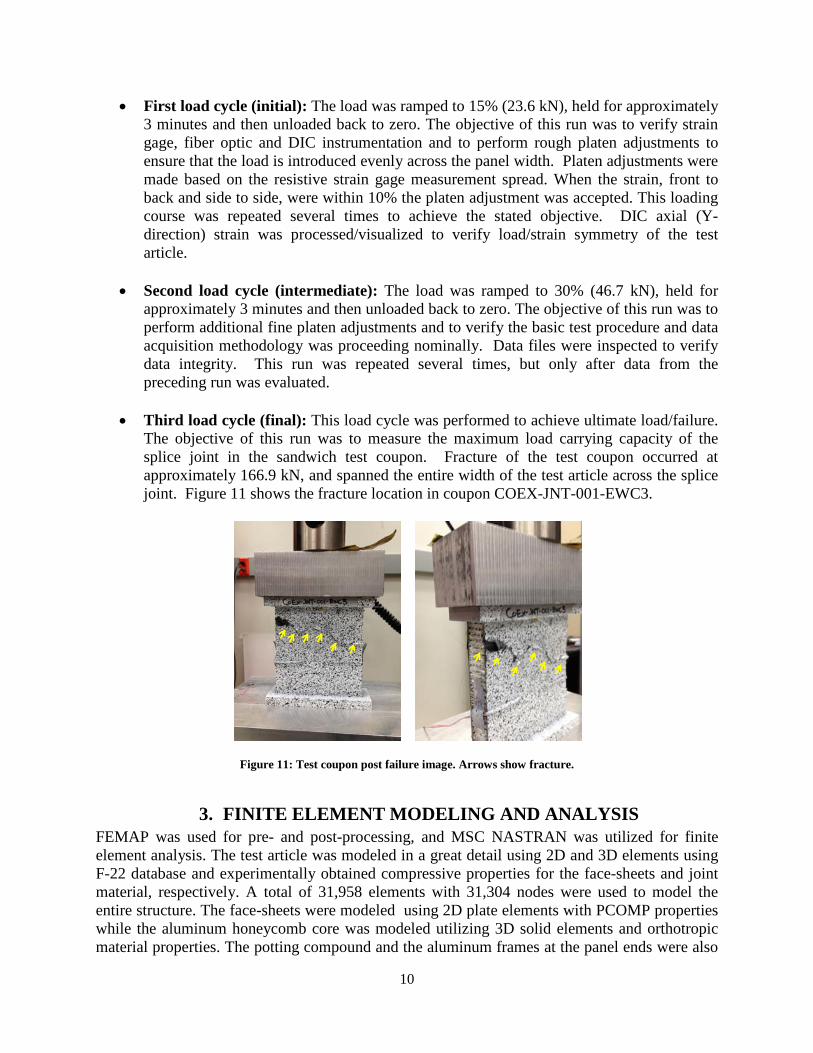
• Third load cycle (final): This load cycle was performed to achieve ultimate load/failure. The objective of this run was to measure the maximum load carrying capacity of the splice joint in the sandwich test coupon. Fracture of the test coupon occurred at approximately 166.9 kN, and spanned the entire width of the test article across the splice joint. Figure 11 shows the fracture location in coupon COEX-JNT-001-EWC3.

Figure 11: Test coupon post failure image. Arrows show fracture.

3. FINITE ELEMENT MODELING AND ANALYSIS FEMAP was used for pre- and post-processing, and MSC NASTRAN was utilized for finite element analysis. The test article was modeled in a great detail using 2D and 3D elements using F-22 database and experimentally obtained compressive properties for the face-sheets and joint material, respectively. A total of 31,958 elements with 31,304 nodes were used to model the entire structure. The face-sheets were modeled using 2D plate elements with PCOMP properties while the aluminum honeycomb core was modeled utilizing 3D solid elements and orthotropic material properties. The potting compound and the aluminum frames at the panel ends were also

11

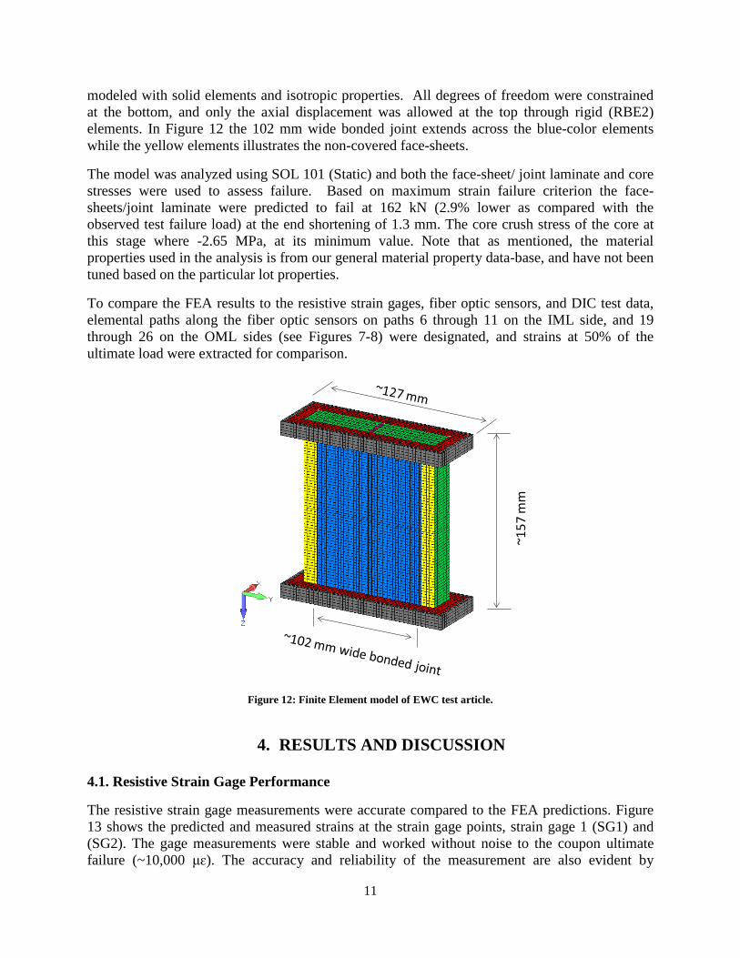
modeled with solid elements and isotropic properties. All degrees of freedom were constrained at the bottom, and only the axial displacement was allowed at the top through rigid (RBE2) elements. In Figure 12 the 102 mm wide bonded joint extends across the blue-color elements while the yellow elements illustrates the non-covered face-sheets.

The model was analyzed using SOL 101 (Static) and both the face-sheet/ joint laminate and core stresses were used to assess failure. Based on maximum strain failure criterion the face-sheets/joint laminate were predicted to fail at 162 kN (2.9% lower as compared with the observed test failure load) at the end shortening of 1.3 mm. The core crush stress of the core at this stage where -2.65 MPa, at its minimum value. Note that as mentioned, the material properties used in the analysis is from our general material property data-base, and have not been tuned based on the particular lot properties.

To compare the FEA results to the resistive strain gages, fiber optic sensors, and DIC test data, elemental paths along the fiber optic sensors on paths 6 through 11 on the IML side, and 19 through 26 on the OML sides (see Figures 7-8) were designated, and strains at 50% of the ultimate load were extracted for comparison.

Figure 12: Finite Element model of EWC test article.

4. RESULTS AND DISCUSSION 4.1. Resistive Strain Gage Performance

The resistive strain gage measurements were accurate compared to the FEA predictions. Figure 13 shows the predicted and measured strains at the strain gage points, strain gage 1 (SG1) and (SG2). The gage measurements were stable and worked without noise to the coupon ultimate failure (~10,000 μɛ). The accuracy and reliability of the measurement are also evident by

~157

mm

12

observing nearly identical readings through SG1 and SG2 (~ 2% difference in the strain-load slopes). SG1 and SG2 are on the IML, along with DIC and the fiber optic sensors, and are the baseline for comparison of the other two systems.

Two of the eight installed resistive gages became inoperative during instrumentation. One soldering pad became disassociated from the backing, and the other disbonded from the substrate. We chose not to replace these and tested with the six remaining resistance strain gages. Resistance strain gage rework and process costs can be seen even in this small test.

Figure 13: SG1 and SG2 strains compared with FEA predictions.

4.2. Full-Field Strain Comparison

Figures 14 through 16 illustrate the DIC images of the loaded sample prior to failure (at 166.9 kN) comparing the axial displacement, axial strain, and hoop strain with the FEA predictions, respectively. The scales in both the DIC images and FEA contours are identical to make the comparison relevant. As it can be seen, the FEA predictions agree very well with the DIC collected data. As mentioned before one of the main advantage of using the DIC system is for validating the finite element analysis, which has been further demonstrated here. The symmetry of the DIC images also verifies that the specimen was loaded and constrained properly which resulted in a uniformly distributed load throughout the specimen. These results also show the ultimate strain capacity of the jointed coupon (~ 10,000 μɛ); and the fact that, he bonded joint remained intact onto the parent structure until the ultimate failure around 166.9 kN.

y = 0.0175x + 1.2678y = 0.0179x + 1.2954

0

20

40

60

80

100

120

140

160

180

0 2000 4000 6000 8000 10000 12000

Axia

l Loa

d, k

N

Axial Strain (μɛ)

SG1

SG2

FEA Prediction (SG1 and SG2)Linear (SG1)

Linear (SG2)

13

Figure 14: Axial displacement at 166.9kN; left: DIC data, right: FEA prediction.

Figure 15: Axial strain at 166.9kN; left: DIC data, right: FEA prediction.

Figure 16: Hoop strain at 166.9kN; left: DIC data, right: FEA prediction.

-1.4 mm

-0.2 mm

mm/mm

mm/mm

14

4.3. Single Point Strain Comparison

In order to compare the performance of Luna’s fiber optic sensing system to resistive strain gages, the percentage difference between each strain gage and coincident fiber locations were calculated for both the IML (Table 1a) and OML (Table 1b) surfaces, respectively. Fiber optic measurements were taken from single points along the fiber optic, on either side of each resistive strain gage, from positions longitudinally and latitudinally collocated with each resistive strain gage. The percentage difference as shown was calculated at five different loading states for each resistive strain gage, with additional comparison given for FEA strains at 50% loading, as well as DIC on the IML surface. As it can be seen from these tables, the percentage difference across measurement methods generally lies below 8%.

Overall, fiber optic sensor measurements display good correlations with resistive strain gage measurements, with the average absolute percentage difference across all locations and loading states calculated to be 4.15%, discarding obvious outliers that occur at the location coincident with SG8 (outliers are discussed more extensively in section 4.5). While great care was taken to bond the fiber as close to each resistive strain gage as possible, it is physically impossible to locate strain gages and fiber at exactly the same location. Therefore some difference in measurement is expected due to strain gradients across the panel, in both the axial and hoop direction. An inspection of our FEA results at the center-line strain gage locations, show a 1%< and 0.04% strain gradient for the adjacent elements, top-bottom and side, of the strain gage elements, respectively.

FEA and DIC strain values also show good agreement to resistive strain gage data. The average absolute percentage difference is 2.77% and 2.57% for FEA and DIC data, respectively.

Table 1a: IML – percentage difference between strain gage readings and fiber optic, DIC, and FEA measurements.

Percent Loading 13% 25% 50% 75% 96%

Msrmt. Method Fiber Fiber DIC Fiber DIC FEA Fiber DIC Fiber

SG1 Latitude 5.01 3.03 -1.27 0.57 -0.26 1.74

Longitude 4.01 2.77

2.90

3.36

1.00

SG2 Latitude 2.39 -1.75 -2.20 1.33 3.49 2.38 1.77 0.29 0.51

Longitude 4.28 -0.55

-1.68

-5.29

-5.33

4.4. Line Strain Comparison

To have a better comparison between the DIC data, fiber optic sensor readings, and the FEA predictions, strains along the mounted fiber optic sensors were tracked and plotted together for selected paths at 50% of the ultimate load. The DIC and FEA axial strains were extracted for paths 6 through 11 on the IML side of the test article (see also Figure 7). Figures 17 a-c show

15

the comparisons for the selected paths along the length of the sample. Figure 18 a-b on the other hand, show the strains on the OML side, comparing the FEA results to the fiber optic sensor measurements (see also Figure 8) . Note that the DIC system was only used on the IML surface. Figure 18 a shows the axial strains along paths 19 through 22 while Figure 18 b illustrates hoop strain along paths 25 and 26. The solid lines, dashed lines, and symbols show the FEA predication, DIC strains, and fiber optic sensors reading, respectively.

Overall, the DIC strains and the strains measured by the fiber optic sensors matched the FEA predicted values very well. Note the excellent correlation in all plots of Figure 17 and Figure 18. However, some oscillations were observed in both the DIC and fiber optic sensor data.

Table 1b: OML – percentage difference between strain gage reading and fiber optic and FEA measurements.

Percent Loading 13% 25% 50% 75% 96%

Msrmt. Method Fiber Fiber Fiber FEA Fiber Fiber

SG3

Latitude 6.72 -3.08 -0.28 3.96 -0.90 -2.23

Latitude 0.95 -1.49 -5.86

-2.73 -5.65

Longitude 7.08 3.63 1.60

-21.10 0.18

SG4

Latitude 7.20 2.77 -2.27 2.85 -0.33 -2.89

Latitude 0.25 -3.50 -4.99

-3.50 -2.80

Longitude -1.00 -2.11 -1.67

11.02 -1.26

SG5

Latitude 5.86 3.82 -0.76 -0.69 -5.41 -2.33

Latitude 0.36 -1.07 -5.94

-4.60 -4.45

Longitude -4.95 -7.30 -7.81 2.90 -7.90

SG8

Latitude -0.93 -4.89 -5.57 6.17 -7.28 -9.08

Latitude -7.82 -8.60 72.78

85.05 83.38

Longitude -6.00 -8.60 -9.20

-14.51 10.14

The minor DIC oscillations are mainly due to the lower resolution of the measurement technique itself (to be around 200 μɛ) and also the non-homogenous nature of the composite material (textured surface) that governs the point strain values at particular locations. As mentioned, an equivalent gage length for the DIC technique is 3.7 mm; this is smaller than 5 mm gage length of the fiber optic sensors, resulting in collecting more localized (non-averaged) strain data as compared with the fiber optic sensors (and the resistive strain gages). As it can also be seen from

16

Figure 17a-c, major disturbances are also evident for the DIC data at ~4.4 cm in Figure 17 a, and around 7 cm in Figure 17b-c, where mainly due to strain gages' lead-wires the speckled pattern was not tracked by the DIC system properly. This is clearly shown in Figure 17 d where the lead-wires created defective regions on the speckled surface.

Further, the DIC system shows a much smoother reading along path 11 (Figure 12 c) where the speckled pattern is on the unidirectional tape face-sheet material with a more homogenized surface texture, as opposed to the 10.2 cm wide joint woven fabric material in the specimen's middle part (including paths 6 through 10).

Figure 17: a,b, c IML data comparisons d) IML DIC images showing non-trackable regions.

The fiber optic sensor data also show some oscillations and outliers, especially at the beginnings and ends of the paths where they transition from bonded to non-bonded regions. Path 21 fiber optic data shows the highest number of outliers among the selected paths since the fiber had to be glued in sections between the three resistive strain gages (see Figure 9). Similar to DIC, the fiber optic sensor shows a much smoother reading along path 11 (Figure 12 c).

4.5. Fiber Data Parameters

The fiber optic sensor data shows good correlation with both strain gage and DIC measurements, as demonstrated in Sections 4.3 and 4.4. However, considering the fiber optic strain sensor is the newest of the techniques used in this study, we choose to delve more deeply into the parameters that govern fiber sensor data, for the benefit of future users.

0 2 4 6 8 10-10000

-8000

-6000

-4000

-2000

0

2000

Location along Axial Direction, cm

Axi

al S

train

, µε

FEA, Path 11Fiber Optic, Path 11DIC, Path 11

0 2 4 6 8 10-10000

-8000

-6000

-4000

-2000

0

2000

Location along Axial Direction, cm

Axi

al S

train

, µε

FEA, Path 6Fiber Optic, Path 6DIC, Path 6FEA, Path 7Fiber Optic, Path 7DIC, Path 7

0 2 4 6 8 10-10000

-8000

-6000

-4000

-2000

0

2000

Location along Axial Direction, cm

Axi

al S

train

, µε

FEA, Path 8 Fiber Optic, Path 8-1Fiber Optic, Path 8-2DIC, Path 8FEA, Path 9Fiber Optic, Path 9DIC, Path 9FEA, Path 10Fiber Optic, Path 10DIC, Path 10

a)

c)

b)

d)

17

Figure 18: OML data comparisons a) axial strains b) hoop strains. Note that the ends of the Fiber Optic Paths that register zero strain has likely come unbonded.

A representative plot of fiber optic sensor measurement over time is shown in Figure 19 as compared to the resistive strain SG2 reading. The figure shows the measurement correlation over time for both these measurement methods. An interesting feature of the composite surface that is picked up by the fiber is the non-uniformity of strain across the cross-weaves of the composite fabric joint material. As the fiber sensor gage length (5mm) is larger than the period of the cross weaves, the Luna system picks this up as a toggling of measured strain values at various points over time, as shown more clearly in the Figure 19 inserts. When the whole 5 mm gage length experiences a largely uniform strain, the cross-correlation produces a single peak, the wavelength shift of which corresponds to the average strain experienced by this region. It is hypothesized that as distinct strain regions form within the gage length, the spectral cross-correlation produces multiple peaks corresponding to multiple strain regions. A maximum peak detection algorithm is used to select the stronger peak and the toggling between two values as seen here is due to the similar strength of the cross-correlation peaks. The use of gage lengths smaller than the periodicity of the cross-weaves will remove this effect and instead capture the fidelity of the weave itself [Gifford 2011].

As mentioned at the end of Section 4.4, as with DIC, textural variation in the surface that the fiber is bonded onto also appears to feed into outlier percentage. The effect of this is seen when comparing the fibers bonded at the edges of the IML over unidirectional tape face-sheet material (path 1 and 11) with straight paths down the middle of the IML over the woven fabric material (path 2, 3, 5, 6, 7, 9, 10). The unidirectional composite tape material has a smoother surface as compared with their woven fabric counterparts. Therefore the expectation is that the edge fiber sensors should show less outliers than the middle fiber sensors. A comparison of these two groups bears this out, with an outlier rate of 1.98% versus 4.43% for edge fiber sensors versus middle ones, respectively. Figure 19 also shows some obviously anomalous outliers especially with higher load, towards the end of the load cycle. The distribution of outliers with strain and location along the fiber is further illustrated in Figures 20 and 21.

0 2 4 6 8 10-12000

-10000

-8000

-6000

-4000

-2000

0

2000

Location along Axial Direction, cm

Axia

l Stra

in, µε

FEA, Path 19Fiber Optic, Path 19FEA, Path 20Fiber Optic, Path 20FEA, Path 21Fiber Optic, Path 21-1Fiber Optic, Path 21-2Fiber Optic, Path 21-3Fiber Optic, Path 21-4FEA, Path 22Fiber Optic, Path 22

0 2 4 6 8 10 12-2000

-1000

0

1000

2000

3000

4000

Location along Hoop Direction, cm

Hoo

p St

rain

, µε

FEA, Path 25Fiber Optic, Path 25FEA, Path 26Fiber Optic, Path 26

a) b)

18

Figure 19: Resistive strain gage comparison to coincident fiber.

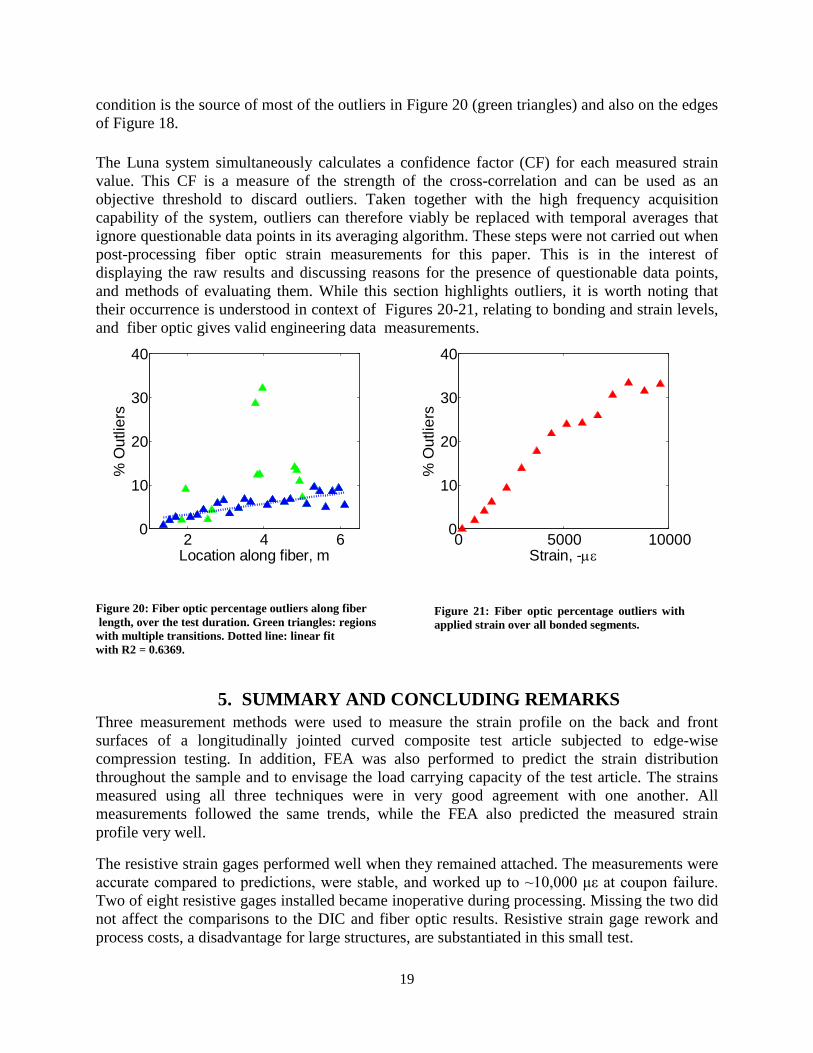
Mathematically, the probability of outliers increases when the cross-correlation of the spectral content within the gage length is of poor quality, resulting in a low signal to noise ratio (SNR). There are a few physical reasons for poor quality spectral information. The algorithm presumes a constant strain across each gage. Consequently, a strain variation or strain gradient could result in a deterioration of SNR. In Figure 19, the strain difference within the 5mm gage length increases with load, from 165 με compared to 280 με for insets (a) and (b), respectively. This increase in strain variation with applied load could be the source of increased outliers at higher strain measurements (Figure 21). Vibrations of higher frequency than the base system acquisition rate (100 Hz for the system used herein) can adversely affect the cross-correlation quality. If the sensor is changing length within a single scan cycle, as caused by high frequency mechanical or acoustical vibrations, the cross correlation can become broadened, leading to a low SNR. The effect of vibration is known to be cumulative down the length of the fiber [Sang 2012]. The algorithm currently implemented corrects for vibration seen on the fiber leading up to the beginning of the sensor. However, any vibration along the sensing length after this point is accumulated, resulting in increased probability of outliers as one progresses down the fiber when vibration is present. This is evidenced in Figure 20 where the outlier percentage increases down the length of the fiber (dotted line linear fit with R2 = 0.6369), though its occurrence is still below 10% at the fiber extreme. The user’s preparation of the experimental setup also plays a role in determining the quality of data output by the system. In this experimental setup, the longitudinal fiber runs between strain gages were particularly challenging to install as it involved routing many short fiber runs (see path 21 in Figure 8a). Compared to fiber runs that span the height of the specimen, in these regions, the 5 mm gage lengths experience high strain gradients as the fiber transitions from bonded (strained) to unbonded (zero strain) regions multiple times. It should be noted that 5mm regions along the sensor where the fiber transitions between bonded and unbonded necessarily violate the physical assumption of a bonded sensor and are not valid measurement points. This

19

condition is the source of most of the outliers in Figure 20 (green triangles) and also on the edges of Figure 18. The Luna system simultaneously calculates a confidence factor (CF) for each measured strain value. This CF is a measure of the strength of the cross-correlation and can be used as an objective threshold to discard outliers. Taken together with the high frequency acquisition capability of the system, outliers can therefore viably be replaced with temporal averages that ignore questionable data points in its averaging algorithm. These steps were not carried out when post-processing fiber optic strain measurements for this paper. This is in the interest of displaying the raw results and discussing reasons for the presence of questionable data points, and methods of evaluating them. While this section highlights outliers, it is worth noting that their occurrence is understood in context of Figures 20-21, relating to bonding and strain levels, and fiber optic gives valid engineering data measurements.

Figure 20: Fiber optic percentage outliers along fiber length, over the test duration. Green triangles: regions with multiple transitions. Dotted line: linear fit with R2 = 0.6369.

5. SUMMARY AND CONCLUDING REMARKS Three measurement methods were used to measure the strain profile on the back and front surfaces of a longitudinally jointed curved composite test article subjected to edge-wise compression testing. In addition, FEA was also performed to predict the strain distribution throughout the sample and to envisage the load carrying capacity of the test article. The strains measured using all three techniques were in very good agreement with one another. All measurements followed the same trends, while the FEA also predicted the measured strain profile very well.

The resistive strain gages performed well when they remained attached. The measurements were accurate compared to predictions, were stable, and worked up to ~10,000 με at coupon failure. Two of eight resistive gages installed became inoperative during processing. Missing the two did not affect the comparisons to the DIC and fiber optic results. Resistive strain gage rework and process costs, a disadvantage for large structures, are substantiated in this small test.

2 4 60

10

20

30

40

Location along fiber, m

% O

utlie

rs

0 5000 100000

10

20

30

40

Strain, -µε

% O

utlie

rs

Figure 21: Fiber optic percentage outliers with applied strain over all bonded segments.

20

DIC can report all components of strain and displacement for the entire observed surface, which is highly beneficial when validating finite element models. It is also non-contact and scale independent. The anomalies (high magnitude oscillations) in the DIC data here were mainly found to be the results of attaching the resistive strain gages' lead-wires on the speckled surface, and some to a small effective strain "gage length" of 3.68 mm for this measurement.

Fiber optic sensing utilizes off-the-shelf, unaltered optical fibers as the sensor, making the sensor inexpensive. This method enables the entire fiber to act as a sensor and allows for hundreds of closely spaced sensing points per meter of fiber. The area coverage and spatial resolution make fiber sensing a useful method of validating model predictions. Fiber strain spuriosity in the data presented here was primarily due to poor quality spectral information as a consequence of a coarse attachment surface texture relative to the system gage length or fiber transitioning from a bonded to a non-bonded region (or vice-versa).

This work lays the foundation for user selection of strain measurement method most suitable to the intended application.

6. ACKNOWLEDGEMENTS To the CoEx team who entrusted us to work for the advancement of joints technology and who performed the joints development with us: Michael Akkerman: NASA/ Goddard Space Flight Center, Ron Glenn and Harry Wilems: NASA/ Goddard Space Flight Center, Sotiris Kellas: NASA/Langley Research Center, Tom Krivanek: NASA/ Glenn Research Center, Larry Pelham: NASA/Marshall Space Flight Center, Ben Rodini: NASA/ Goddard Space Flight Center, Mark Shuart : NASA/Langley Research Center, James Sutter: NASA/Glenn Research Center.

7. REFERENCES • Soller, Brian, Gifford, Dawn, Wolfe, Matthew, and Froggatt, Mark. “High resolution optical

frequency domain reflectometry for characterization of components and assemblies.” Optics Express 13 (2005): 666-674.

• Soller, B. J., Wolfe, M., and Froggatt, M. E. “Polarization resolved measurement of Rayleigh backscatter in fiber-optic components.” Optical Fiber Communication Conference and Exposition and the National Fiber Optic Engineers Conference Technical Digest. Anaheim, California, March 6, 2005. Optical Society of America, 2005. Paper NWD3. CD-ROM.

• Davis, Michael A., and Kersey, Alan D. “Simultaneous measurement of temperature and strain using fiber Bragg gratings and Brillouin scattering.” Proc. SPIE 2838 (1996): 114-123.

• Froggatt, Mark, and Moore, Jason. “High resolution strain measurement in optical fiber with Rayleigh scatter.” Appl. Opt. 37 (1998): 1735-1740.

• Froggatt, M., Soller, B., Gifford, D., and Wolfe, M. “Correlation and keying of Rayleigh scatter for loss and temperature sensing in parallel optical networks.” Optical Fiber Communication Conference, 2004 Technical Digest. Los Angeles, California, February 23-27, 2004. Optical Society of America, 2004. Paper PD17. CD-ROM -3 pp.

• Soller, B. J., Gifford, D. K., Wolfe, M. S., Froggatt, M. E., Yu, M. H., and Wysocki, P. F. “Measurement of localized heating in fiber optic components with millimeter spatial

21

resolution.” Optical Fiber Communication Conference and Exposition and the National Fiber Optic Engineers Conference Technical Digest. Anaheim, California, March 5-10, 2006. Optical Society of America, 2006. Paper OFN 3. CD-ROM -3 pp.

• Guemes, Alfredo, Fernandez-Lopez, Antonio, and Soller, Brian. “Optical Fiber Distributed Sensing – Physical Principles and Applications.” Structural Health Monitoring 9 (3) (2010): 233-245.

• Kaplan, A., Klute, S. M., and Heaney, A. “Distributed Optical Fiber Sensing for Wind Blade Strain Monitoring and Defect Detection.” Proceedings of the 8th International Workshop on Structural Health Monitoring. Stanford, California, Sept. 13-15, 2011. Stanford University, 2011. CD-ROM.

• Klute, S. M., Gifford, D. K., Sang., A. K., and Froggatt, M. E. “Defect Detection During Manufacture of Composite Wind Turbine Blade with Embedded Fiber Optic Distributed Strain Sensor.” Proceedings of the 43rd International SAMPE Tech. Conf. Ft. Worth, Texas, Oct. 17-20, 2011. Society for the Advancement of Material and Process Engineering. CDROM- 15 pp.

• Pedrazzani, J. R., Klute, S. M., Gifford, D. K., Sang., A. K., and Froggatt, M. E. “Embedded and surface mounted fiber optics sensors detect manufacturing defects and accumulated damage as a wind turbine blade is cycled to failure.” SAMPE 2012 Technical Conference Proceedings: Emerging Opportunities: Materials and Process Solutions. Baltimore, MD, May 21-24, 2012. Society for the Advancement of Material and Process Engineering. CDROM expected.

• Pedrazzani, J.R., Castellucci, M., Sang, A.K., Froggatt, M.E., Klute, S.M., Gifford, D.K. “Fiber Optic Distributed Strain Sensing Used to Investigate the Strain Fields in a Wind Turbine Blade and in a Test Coupon with Open Holes.” SAMPE Tech. Conf. 2012. Charleston, South Carolina, Oct. 22-25, 2012. Society for the Advancement of Material and Process Engineering. CDROM expected.

• Sang, A.K. “Distributed Vibration Sensing using Rayleigh Backscatter in Optical Fibers.” PhD Thesis. 2011. Virginia Polytechnic Institute and State University.

• Gifford, D. K., Metrey, D. R., Froggatt, M. E., Rogers, M. E., Sang, A. K.. “Monitoring Strain During Composite Manufacturing Using Embedded Distributed Optical Fiber Sensing”. SAMPE 2011. Long Beach, CA. Society for the Advancement of Material and Process Engineering.